Embed Size (px)
Citation preview

Commit Write Facility; dml1.sqlAuthor: Craig Shallahamer ([email protected]), Version 1f, 17-Feb-2012.
Background and Purpose
The purpose of this notepad is to see if using Oracle’s commit write facility increases performance measured by a decreasein response time (ms/commits) and increase in arrival rate.
Because it can be difficult to compare the response times when the arrival rate changes, at the bottom of the notebook Icomplete the relationship between work and time, and then set the work to be same then derived the response time. Thisallows a pretty good apples-to-apples comparision.
The data used in the notebook is based on the dml1.sql script, which creates a heavy CPU load and a light IO load on thesystem. But the top wait event during the wait,immediate option is still log file sync.
The terminalolgy used is a mix of queury theory and Oracle database-ease. Without getting into details, CPU time per unit ofwork is equal to the service time, the non-idle wait time per unit of work is the queue time, and respons time is service timeplus queue time. Key to understanding this is knowing the time is based on a single unit of work. For this experiment thechosen unit of work was the Oracle statistic “user commit”. Every commit issued by an Oracle client/user process will tick-upthe user commit statistics. As a result, the user commit is a very good unit of work when understanding the commit rate of anapplication or workload.
Experimental Data
Below is all the experimental data. The experiment was run on a Dell single four-core CPU, Oracle 11.2G. According to “cat/proc/version”: Linux version 2.6.18-164.el5PAE ([email protected]) (gcc version 4.1.2 20080704 (RedHat 4.1.2-46)) #1 SMP Thu Sep 3 02:28:20 EDT 2009. There was an intense DML update load by five sessions. The DML script is dml1.sql, which in the experimental enviromentcause a severe CPU bottleneck and then some log file sync time. The CPU consumption was many, many times more thanthe wait time. This can be seen far below, by comparing the average CPU per commmit compared to the average wait timeper commit.
After each update and commit, there was a subsecon lognomal distirbuted sleep time. During each of the data collectionperiods, the follow data was gathered. The percentage figures were visually observed and recorded.
Grid@88"Setting", "Commitêsec", "CPU %","log file sync\nWait Time %", "log file par write\nWait Time %"<,
8"wait immediate", "8.32", "98%", "48%", "38%"<,8"wait batch", "8.46", "98%", "53%", "37%"<,8"nowait batch", "8.47", "99%", "0%", "70%"<,8"nowait immediate", "8.47", "99%", "0%", "13%"<
<, Frame Ø AllD
Setting Commitêsec CPU % log file syncWait Time %
log file par writeWait Time %
wait immediate 8.32 98% 48% 38%wait batch 8.46 98% 53% 37%
nowait batch 8.47 99% 0% 70%nowait immediate 8.47 99% 0% 13%
As you can see below, for each of the four commit write facility options, there were 32, 90 second samples taken.
The order of sample data is sample number, elapsed time (seconds), commits (user commits), instance non-idle wait time(sec), and instance CPU consumption (sec).

As you can see below, for each of the four commit write facility options, there were 32, 90 second samples taken.
The order of sample data is sample number, elapsed time (seconds), commits (user commits), instance non-idle wait time(sec), and instance CPU consumption (sec).
ssWaitImmediate = 81, 90.016833, 771, 19.99, 354.364125, 2, 90.033525, 749, 17.87, 354.691076, 3,90.008822, 773, 21.36, 350.727679, 4, 90.013937, 751, 22.03, 346.919255, 5, 90.018566, 731,20.81, 350.842663, 6, 90.011928, 758, 20.78, 354.665081, 7, 90.018995, 703, 18.66, 354.482108,8, 90.01774, 760, 21.02, 354.027181, 9, 90.009464, 748, 21.74, 354.479108, 10, 90.009953, 731,20.36, 350.538708, 11, 90.014985, 765, 22.67, 354.848052, 12, 90.011934, 749, 20.76, 347.112231,13, 90.127603, 734, 21.82, 355.003026, 14, 90.034552, 782, 18.93, 358.275535, 15, 90.017466, 760,21.59, 354.611091, 16, 90.007765, 725, 18.74, 349.996791, 17, 90.181153, 737, 21.2, 354.792059,18, 90.016256, 733, 20.15, 346.241361, 19, 90.015182, 753, 19.65, 353.121318, 20, 90.015107, 734,18.79, 352.353429, 21, 90.007711, 739, 23.59, 352.740372, 22, 90.012739, 719, 19.95, 352.312437,23, 90.013051, 758, 21.24, 348.47902, 24, 90.028347, 765, 20.94, 354.810059, 25, 90.005068, 757,20.21, 346.68229, 26, 90.015379, 786, 22.92, 354.465113, 27, 90.013851, 751, 23.76, 354.618089,28, 90.016416, 747, 19.47, 358.364517, 29, 90.015136, 723, 20, 355.046019, 30, 90.027755, 757,21.76, 354.118158, 31, 90.018465, 736, 19.13, 347.09023, 32, 90.015684, 783, 20.79, 350.503711<;
ssWaitBatch = 81, 90.012865, 774, 22.6, 358.332522, 2, 90.008947, 800, 21.06, 355.045021, 3,90.017088, 758, 21.58, 355.118006, 4, 90.127519, 766, 20.55, 354.750064, 5, 90.102755, 758,19.97, 362.216932, 6, 90.018209, 780, 22.16, 350.464718, 7, 90.009452, 752, 20.37, 346.508324,8, 90.014387, 745, 19.89, 354.683074, 9, 90.005624, 787, 21.59, 354.466105, 10, 90.013743, 734,20.27, 354.671084, 11, 90.25017, 779, 19.93, 355.018023, 12, 90.014355, 740, 21.23, 347.152222,13, 90.007112, 763, 21.49, 354.397123, 14, 90.045861, 755, 19.64, 362.34791, 15, 90.096495, 750,19.92, 350.322742, 16, 90.009461, 783, 22.79, 354.400121, 17, 90.005002, 752, 19.87, 354.659082,18, 90.178983, 770, 22.42, 354.747066, 19, 90.008779, 742, 21.12, 351.146615, 20, 90.032213, 754,21.07, 354.689078, 21, 90.013209, 752, 20.24, 354.948034, 22, 90.013705, 738, 19.6, 350.747672,23, 90.05598, 770, 20.74, 354.680078, 24, 90.017555, 740, 19.09, 354.166153, 25, 90.130722, 769,21.93, 359.919283, 26, 90.043504, 749, 22.23, 354.775064, 27, 90.008103, 760, 20.05, 346.497318,28, 90.036155, 802, 21.51, 354.282141, 29, 90.010146, 743, 18.66, 355.071018, 30, 90.14741, 784,20.61, 354.73207, 31, 90.071883, 790, 20.73, 358.664473, 32, 90.040811, 734, 19.8, 354.707074<;
ssNowaitImmediate = 81, 90.009553, 767, .81, 356.866744, 2, 90.019994, 783, .51, 357.144702,3, 90.019171, 770, .64, 357.324679, 4, 90.021457, 796, .45, 357.037716, 5, 90.008423, 770,.53, 361.16009, 6, 90.008982, 752, .54, 356.940735, 7, 90.019636, 822, 15.07, 355.901891,8, 90.010252, 752, .44, 356.987728, 9, 90.011047, 789, .62, 353.240297, 10, 90.009254, 751,.51, 357.439661, 11, 90.019374, 734, 3.09, 360.610173, 12, 90.015876, 734, .38, 355.347976,13, 90.01989, 739, .48, 352.75137, 14, 90.010219, 746, .77, 346.632299, 15, 90.008739, 753,.45, 346.246359, 16, 90.019661, 751, .36, 350.176761, 17, 90.019855, 818, .56, 354.17415,18, 90.01924, 760, .47, 357.274682, 19, 90.007998, 762, .51, 357.428658, 20, 90.010544, 778,.5, 357.219693, 21, 90.009052, 785, .44, 357.237689, 22, 90.021595, 764, .57, 356.870745,23, 90.01029, 777, .5, 357.269683, 24, 90.019274, 747, .57, 356.839753, 25, 90.008304, 739,.39, 352.970341, 26, 90.009707, 756, .42, 349.240906, 27, 90.008482, 753, .4, 350.541707, 28,90.012067, 755, .49, 353.878196, 29, 90.017928, 761, .61, 349.937801, 30, 90.008913, 744,.65, 349.2599, 31, 90.009847, 750, .35, 349.267899, 32, 90.008737, 750, .52, 355.206999<;
ssNowaitBatch = 81, 90.020026, 770, .1, 357.219694, 2, 90.012683, 774, .1, 356.704768, 3,90.019968, 774, .13, 357.184694, 4, 90.020716, 736, .18, 357.260685, 5, 90.010322, 764,.1, 352.88535, 6, 90.009205, 721, .07, 349.190912, 7, 90.010882, 764, .16, 354.696071, 8,90.020235, 781, .07, 357.380669, 9, 90.008057, 765, .15, 356.88574, 10, 90.00892, 759, .22,356.866741, 11, 90.008881, 747, .16, 357.053721, 12, 90.019757, 768, .19, 357.088711, 13,90.019939, 753, .25, 357.274684, 14, 90.020031, 738, .2, 357.050717, 15, 90.019802, 787, .1,356.964727, 16, 90.008867, 778, .08, 357.258683, 17, 90.009095, 773, .17, 357.196697, 18,90.021109, 759, .22, 352.730374, 19, 90.009436, 761, .13, 357.308677, 20, 90.008822, 768,.13, 357.176699, 21, 90.008863, 753, .13, 357.222692, 22, 90.009543, 735, .09, 356.835751,23, 90.009349, 793, .21, 356.587787, 24, 90.020508, 767, .16, 356.848753, 25, 90.009135, 761,.13, 360.342215, 26, 90.008955, 787, .11, 354.730069, 27, 90.008543, 758, .14, 352.981338,28, 90.010361, 753, .2, 356.89174, 29, 90.019722, 748, .09, 357.274682, 30, 90.020663, 791,.38, 357.702619, 31, 90.009318, 742, .06, 353.872199, 32, 90.008455, 769, .2, 349.396881<;
Data Loading
All the data sets are contained in the above section.
2 CW_Analysis_dml1_1f.nb

ssNum = 4;sampleNum = 32;ss@1D = ssWaitImmediate; ssName@1D = "Wait Immediate";ss@2D = ssWaitBatch; ssName@2D = "Wait Batch";ss@3D = ssNowaitImmediate; ssName@3D = "Nowait Immediate";ss@4D = ssNowaitBatch; ssName@4D = "Nowait Batch";
ncols = 5;sampleCol = 1;elapsedTCol = 2;workCol = 3;waitTCol = 4;cpuTCol = 5;
Do@ssWork@ssidxD = 8<; ssL@ssidxD = 8<; ssSt@ssidxD = 8<; ssQt@ssidxD = 8<; ssRt@ssidxD = 8<;theSS = ss@ssidxD;Table@elapsedT = theSS@@ncols sampleidx + elapsedTColDD;workTot = theSS@@ncols sampleidx + workColDD;cpuSecTot = theSS@@ncols sampleidx + cpuTColDD;waitSecTot = theSS@@ncols sampleidx + waitTColDD;H*Print@ssidx," ",sampleidx," elapsedT=",elapsedTD;*L
l = workTot ê H1000 elapsedTL;St = HcpuSecTot 1000L ê workTot;Qt = HwaitSecTot 1000L ê workTot;Rt = St + Qt;
AppendTo@ssWork@ssidxD, workTotD;AppendTo@ssL@ssidxD, lD;AppendTo@ssSt@ssidxD, StD;AppendTo@ssQt@ssidxD, QtD;AppendTo@ssRt@ssidxD, RtD;
, 8sampleidx, 0, sampleNum - 1<D;, 8ssidx, ssNum<
D;ssName@1Dss@1DLength@ssWork@1DDTake@ssWork@1D, 5DN@Mean@ssWork@1DDD
Wait Immediate
81, 90.0168, 771, 19.99, 354.364, 2, 90.0335, 749, 17.87, 354.691, 3, 90.0088, 773, 21.36, 350.728, 4,90.0139, 751, 22.03, 346.919, 5, 90.0186, 731, 20.81, 350.843, 6, 90.0119, 758, 20.78, 354.665, 7,90.019, 703, 18.66, 354.482, 8, 90.0177, 760, 21.02, 354.027, 9, 90.0095, 748, 21.74, 354.479, 10,90.01, 731, 20.36, 350.539, 11, 90.015, 765, 22.67, 354.848, 12, 90.0119, 749, 20.76, 347.112, 13,90.1276, 734, 21.82, 355.003, 14, 90.0346, 782, 18.93, 358.276, 15, 90.0175, 760, 21.59, 354.611,16, 90.0078, 725, 18.74, 349.997, 17, 90.1812, 737, 21.2, 354.792, 18, 90.0163, 733, 20.15,346.241, 19, 90.0152, 753, 19.65, 353.121, 20, 90.0151, 734, 18.79, 352.353, 21, 90.0077, 739,23.59, 352.74, 22, 90.0127, 719, 19.95, 352.312, 23, 90.0131, 758, 21.24, 348.479, 24, 90.0283,765, 20.94, 354.81, 25, 90.0051, 757, 20.21, 346.682, 26, 90.0154, 786, 22.92, 354.465, 27,90.0139, 751, 23.76, 354.618, 28, 90.0164, 747, 19.47, 358.365, 29, 90.0151, 723, 20, 355.046, 30,90.0278, 757, 21.76, 354.118, 31, 90.0185, 736, 19.13, 347.09, 32, 90.0157, 783, 20.79, 350.504<
32
8771, 749, 773, 751, 731<
749.
Basic Statistics
CW_Analysis_dml1_1f.nb 3

Basic Statistics
In this section I calculate the basic statistics, such as the mean and median. My objective is to ensure the data has beencollected and entered correctly and also to compare the two datasets to see if they appear to be different.
myData = Table@8ssName@ssidxD, N@Mean@ssWork@ssidxDDD,Mean@ssL@ssidxDD, Mean@ssSt@ssidxDD, Mean@ssQt@ssidxDD, Mean@ssRt@ssidxDD,Length@ssWork@ssidxDD, N@StandardDeviation@ssL@ssidxDDD, N@StandardDeviation@ssSt@ssidxDDD,N@StandardDeviation@ssQt@ssidxDDD, N@StandardDeviation@ssRt@ssidxDDD
<, 8ssidx, 1, ssNum<D;
toGrid = Prepend@myData, 8"Settings", "Avg Work\nHcmtL", "Avg L\nHcmtêmsL","Avg CPUt\nHmsêcmtL", "Avg Wt\nHmsêcmtL", "Avg Rt\nHmsêcmtL", "Samples","Stdev L\nHcmtêmsL", "Stdev CPUt\nHmsêcmtL", "Stdev Wt\nHmsêcmtL", "Stdev Rt\nHmsêcmtL"<D;
Grid@toGrid,Frame ØAllD
SettinÖgs
AvgWork
HcmtL
Avg LHcmtêms
L
AvgCPUt
HmsêcmtL
Avg WtHmsêcmt
L
Avg RtHmsêcmt
L
Samples Stdev LHcmtêms
L
StdevCPUt
HmsêcmtL
StdevWt
HmsêcmtL
StdevRt
HmsêcmtL
WaitImmeÖdiaÖte
749. 0.0083Ö1995
470.976 27.6505 498.626 32 0.0002Ö17009
12.4358 1.80699 12.6189
WaitBatch
761.656 0.0084Ö5821
465.452 27.2719 492.724 32 0.0002Ö10098
11.4239 1.19211 11.4096
NowaitImmeÖdiaÖte
762.75 0.0084Ö7372
465.186 1.33771 466.523 32 0.0002Ö41156
12.6153 3.1666 11.7575
NowaitBatch
762.406 0.0084Ö6991
467.24 0.1968Ö75
467.436 32 0.0001Ö89893
10.2195 0.0844Ö592
10.2097
In this section I calculate the key parameters for understanding the change. The columns heading are a mix of queuingtheory and Oracle-ease centric.
4 CW_Analysis_dml1_1f.nb

myData = Table@8ssName@ssidxD,N@Mean@ssWork@ssidxDDD, N@100 * HMean@ssWork@ssidxDD - Mean@ssWork@1DDL ê Mean@ssWork@1DDD,Mean@ssL@ssidxDD, 100 * HMean@ssL@ssidxDD - Mean@ssL@1DDL ê Mean@ssL@1DD,Mean@ssSt@ssidxDD, 100 * HMean@ssSt@ssidxDD - Mean@ssSt@1DDL ê Mean@ssSt@1DD,Mean@ssQt@ssidxDD, 100 * HMean@ssQt@ssidxDD - Mean@ssQt@1DDL ê Mean@ssQt@1DD,Mean@ssRt@ssidxDD, 100 * HMean@ssRt@ssidxDD - Mean@ssRt@1DDL ê Mean@ssRt@1DD,Length@ssWork@ssidxDD
<, 8ssidx, 1, ssNum<D;
toGrid = Prepend@myData,8"Settings", "Avg Work\nHcmtL", "%\nChange", "Avg L\nHcmtêmsL", "%\nChange", "Avg CPUt\nHmsêcmtL","%\nChange", "Avg Wt\nHmsêcmtL", "%\nChange", "Avg Rt\nHmsêcmtL", "%\nChange", "Samples"<D;
Grid@toGrid,Frame ØAllD
SettiÖngÖs
AvgWork
HcmtL
%Change
Avg LHcmtê
msL
%Change
AvgCPUt
HmsêcmtL
%Change
Avg WtHmsê
cmtL
%Change
Avg RtHmsê
cmtL
%Change
SamplÖes
WaitImmÖedÖiaÖte
749. 0. 0.008Ö3199Ö5
0. 470.9Ö76
0. 27.65Ö05
0. 498.6Ö26
0. 32
WaitBatÖch
761.6Ö56
1.689Ö75
0.008Ö4582Ö1
1.661Ö79
465.4Ö52
-1.17Ö276
27.27Ö19
-1.36Ö94
492.7Ö24
-1.18Ö367
32
Nowait
ImmÖedÖiaÖte
762.75 1.835Ö78
0.008Ö4737Ö2
1.848Ö25
465.1Ö86
-1.22Ö937
1.337Ö71
-95.1Ö621
466.5Ö23
-6.43Ö826
32
Nowait
BatÖch
762.4Ö06
1.789Ö89
0.008Ö4699Ö1
1.802Ö49
467.24 -0.79Ö327Ö6
0.196Ö875
-99.2Ö88
467.4Ö36
-6.25Ö515
32
In this section I’m showing change and if that change is statictially significant, all compared to our baseline sample set,wait,immediate. This is pretty cool: As mentioned in the Normality Tests section below, distributions in a ttest must be nor-mal. If not, then a location test can be performed. If you look closely at the code segment, below I tested and adjusted for this.
CW_Analysis_dml1_1f.nb 5

myData = Table@8ssName@ssidxD,100 * HMean@ssL@ssidxDD - Mean@ssL@1DDL ê Mean@ssL@1DD,If@DistributionFitTest@ssL@ssidxDD ¥ 0.050,TTest@8ssL@1D, ssL@ssidxD<D,LocationEquivalenceTest@8ssL@1D, ssL@ssidxD<D
D,100 * HMean@ssRt@ssidxDD - Mean@ssRt@1DDL ê Mean@ssRt@1DD,If@DistributionFitTest@ssRt@ssidxDD ¥ 0.050,TTest@8ssRt@1D, ssRt@ssidxD<D,LocationEquivalenceTest@8ssRt@1D, ssRt@ssidxD<D
D<, 8ssidx, 1, ssNum<
D;toGrid = Prepend@myData, 8"Settings", "Avg L\n% Change",
"Avg L\nTtest pvalue", "Avg Rt\n% Change", "Avg Rt\nTtest pvalue"<D;Grid@toGrid,Frame ØAllD
Settings Avg L% Change
Avg LTtest pvalue
Avg Rt% Change
Avg RtTtest pvalue
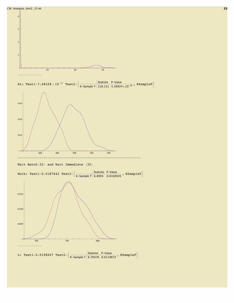
Wait Immediate 0. 1. 0. 1.Wait Batch 1.66179 0.0119672 -1.18367 0.0541915
Nowait Immediate 1.84825 0.0245961 -6.43826 1.95955 µ 10-15
Nowait Batch 1.80249 0.00458214 -6.25515 5.38924 µ 10-16
Sample Set Normality Tests
Before we can perform a standard t-test hypothesis tests on our data, we need to ensure it is normally distributed...becausethat is one of the underlying assumptions and requirements for properly performing a t-test.
Statistical and vlsual normality test
Our alpha will be 0.05, so if the distribution fit test results in a value greater than 0.05 then we can assume the data set isindeed normally distributed.
The first test is just to double check to make sure my thinking is correct. Since I creating a normal distribution based on amean and standard deviation (just happens to be based on the my sample set data), I would expect a p-value (the result) togreatly exceed 0.05. Notice that the more samples I have created (the final number), the closer the p-value approaches 1.0.
6 CW_Analysis_dml1_1f.nb

check = DistributionFitTest@RandomVariate@NormalDistribution@Mean@ssSt@1DD, StandardDeviation@ssSt@1DDD, 10 000DD;
Print@"This number should be much greater than 0.05: ", check," If not try again by re-evaluating."D;
Do@Print@"======================================================================="D;Print@ssName@iD, ", ", Length@ssSt@iDD, " sample values"D;pValueWork = DistributionFitTest@ssWork@iDD;pValueL = DistributionFitTest@ssL@iDD;pValueSt = DistributionFitTest@ssSt@iDD;pValueQt = DistributionFitTest@ssQt@iDD;pValueRt = DistributionFitTest@ssRt@iDD;Print@"Work pvalue=", pValueWorkD;Print@Histogram@ssWork@iD, PlotLabel Ø "Occurances vs Work", AxesLabel Ø 8"Sample value", "Occurs"<DD;
Print@"---------------------------"D;Print@"L pvalue=", pValueLD;Print@Histogram@ssL@iD, PlotLabel Ø "Occurances vs L", AxesLabel Ø 8"Sample value", "Occurs"<DD;Print@"---------------------------"D;Print@"St pvalue=", pValueStD;Print@Histogram@ssSt@iD, PlotLabel Ø "Occurances vs St", AxesLabel Ø 8"Sample value", "Occurs"<DD;Print@"---------------------------"D;Print@"Qt pvalue=", pValueQtD;Print@Histogram@ssQt@iD, PlotLabel Ø "Occurances vs Qt", AxesLabel Ø 8"Sample value", "Occurs"<DD;Print@"---------------------------"D;Print@"Rt pvalue=", pValueRtD;Print@Histogram@ssRt@iD, PlotLabel Ø "Occurances vs Rt", AxesLabel Ø 8"Sample value", "Occurs"<DD;, 8i, 1, ssNum<
D;
This number should be much greater than 0.05: 0.0889051 If not try again by re-evaluating.
=======================================================================
Wait Immediate, 32 sample values
Work pvalue=0.742428
---------------------------
L pvalue=0.687486
CW_Analysis_dml1_1f.nb 7

---------------------------
St pvalue=0.892997
---------------------------
Qt pvalue=0.607359
---------------------------
Rt pvalue=0.823046
=======================================================================
Wait Batch, 32 sample values
Work pvalue=0.273505
8 CW_Analysis_dml1_1f.nb

---------------------------
L pvalue=0.30573
---------------------------
St pvalue=0.448043
---------------------------
Qt pvalue=0.023525
CW_Analysis_dml1_1f.nb 9

---------------------------
Rt pvalue=0.140102
=======================================================================
Nowait Immediate, 32 sample values
Work pvalue=0.0117987
---------------------------
L pvalue=0.0119974
10 CW_Analysis_dml1_1f.nb

---------------------------
St pvalue=0.140427
---------------------------
Qt pvalue=0
---------------------------
Rt pvalue=0.473645
CW_Analysis_dml1_1f.nb 11

=======================================================================
Nowait Batch, 32 sample values
Work pvalue=0.849278
---------------------------
L pvalue=0.849148
---------------------------
St pvalue=0.374021
12 CW_Analysis_dml1_1f.nb
---------------------------
Qt pvalue=0.251681
---------------------------
Rt pvalue=0.380833
Sample Comparison Tests (when normality exists)
Assuming our samples are normally distributed, now it’s time to see if they are significantly different. If so, then we knowchanging the commit write optoins indeed makes a significant performance difference...at least statistically.
The null hypothesis is; there is no real difference between our samples sets. We need to statistically prove that any differ-ence is the result of randomness; like we just happened to pick poor set of samples and it makes their difference look muchworse than it really is.
A t-test will produce a statistic p. The p value is a probability, with a value ranging from zero to one. It is the answer to thisquestion: If the populations really have the same mean overall, what is the probability that random sampling would lead to adifference between sample means larger than observed?
For example, if the p value is 0.03 we can say a random sampling from identical populations would lead to a differencesmaller than you observed in 97% of the experiments and larger than you observed in 3% of the experiments.
Said another way, suppose I have a single sample set and I copy it, resultling in two identical sample sets. Now suppose weperform a significance test on these two identical sample sets. The resuting p-value will be 1.0 because they are exactly thesame. We are essentially doing the same thing here except we have to different sample sets... but we still want to see if they“like” each other..and in our case we hope they are NOT like each other, which means the p-value will low... below our cut offvalue of 0.05.
For our analysis we choose alpha of 0.05. To accept that our two samples are statistically similar the p value would need tobe less than 0.05 (our alpha).
Good reference about the P-Value and significance testing: http://www.graphpad.com/articles/pvalue.htm
Here we go (assuming our samples are normally distributed):
1. Our P value threshold is 0.05, which is our alpha.2. The null hypothesis is the two populations have the same mean. (Remember we have to sample sets, which not thepopulation.)3. Do the statistical test to compute the P value.4. Compare the result P value to our threshold alpha value. If the P value is less then our threshold, we will reject the nullhypothesis and say the difference between our samples is significant. However, if the P value is greater than the threshold,we cannot reject the null hypothesis and any difference between our samples are not statistically significant.
CW_Analysis_dml1_1f.nb 13

Assuming our samples are normally distributed, now it’s time to see if they are significantly different. If so, then we knowchanging the commit write optoins indeed makes a significant performance difference...at least statistically.
The null hypothesis is; there is no real difference between our samples sets. We need to statistically prove that any differ-ence is the result of randomness; like we just happened to pick poor set of samples and it makes their difference look muchworse than it really is.
A t-test will produce a statistic p. The p value is a probability, with a value ranging from zero to one. It is the answer to thisquestion: If the populations really have the same mean overall, what is the probability that random sampling would lead to adifference between sample means larger than observed?
For example, if the p value is 0.03 we can say a random sampling from identical populations would lead to a differencesmaller than you observed in 97% of the experiments and larger than you observed in 3% of the experiments.
Said another way, suppose I have a single sample set and I copy it, resultling in two identical sample sets. Now suppose weperform a significance test on these two identical sample sets. The resuting p-value will be 1.0 because they are exactly thesame. We are essentially doing the same thing here except we have to different sample sets... but we still want to see if they“like” each other..and in our case we hope they are NOT like each other, which means the p-value will low... below our cut offvalue of 0.05.
For our analysis we choose alpha of 0.05. To accept that our two samples are statistically similar the p value would need tobe less than 0.05 (our alpha).
Good reference about the P-Value and significance testing: http://www.graphpad.com/articles/pvalue.htm
Here we go (assuming our samples are normally distributed):
1. Our P value threshold is 0.05, which is our alpha.2. The null hypothesis is the two populations have the same mean. (Remember we have to sample sets, which not thepopulation.)3. Do the statistical test to compute the P value.4. Compare the result P value to our threshold alpha value. If the P value is less then our threshold, we will reject the nullhypothesis and say the difference between our samples is significant. However, if the P value is greater than the threshold,we cannot reject the null hypothesis and any difference between our samples are not statistically significant.
Print@"P-values assumming normality exists."D;Table@
Table@If@i ¹≠ j,
Print@"=============================================================="D;Print@ssName@iD, "H", Length@ssL@iDD, "L and ", ssName@jD, " H", Length@ssL@jDD, "L"D;pValueWork = TTest@8ssWork@iD, ssWork@jD<D;Print@"Work: ", pValueWorkD;pValueL = TTest@8ssL@iD, ssL@jD<D;Print@"L: ", pValueLD;pValueSt = TTest@8ssSt@iD, ssSt@jD<D;Print@"St: ", pValueStD;pValueQt = TTest@8ssQt@iD, ssQt@jD<D;Print@"Qt: ", pValueQtD;pValueRt = TTest@8ssRt@iD, ssRt@jD<D;Print@"Rt: ", pValueRtD;
D;,8j, 1, ssNum<
D;, 8i, 1, ssNum<
D;
P-values assumming normality exists.
==============================================================
Wait ImmediateH32L and Wait Batch H32L
Work: 0.0108505
L: 0.0119672
St: 0.0690354
TTest::nortst : At least one of the p-values in 80.607359, 0.023525<, resulting froma test for normality, is below 0.025`. The tests in 8T< require that the data is normally distributed. à
Qt: 0.326288
Rt: 0.0541915
==============================================================
Wait ImmediateH32L and Nowait Immediate H32L
14 CW_Analysis_dml1_1f.nb

TTest::nortst : At least one of the p-values in 80.742428, 0.0117987<, resulting froma test for normality, is below 0.025`. The tests in 8T< require that the data is normally distributed. à
Work: 0.00980034
TTest::nortst : At least one of the p-values in 80.687486, 0.0119974<, resulting froma test for normality, is below 0.025`. The tests in 8T< require that the data is normally distributed. à
General::stop : Further output of TTest::nortst will be suppressed during this calculation. à
L: 0.00938465
St: 0.0692285
Qt: 1.21047 µ 10-39
Rt: 1.95955 µ 10-15
==============================================================
Wait ImmediateH32L and Nowait Batch H32L
Work: 0.00481099
L: 0.00458214
St: 0.194013
Qt: 1.45446 µ 10-38
Rt: 5.38924 µ 10-16
==============================================================
Wait BatchH32L and Wait Immediate H32L
Work: 0.0108505
L: 0.0119672
St: 0.0690354
Qt: 0.326288
Rt: 0.0541915
==============================================================
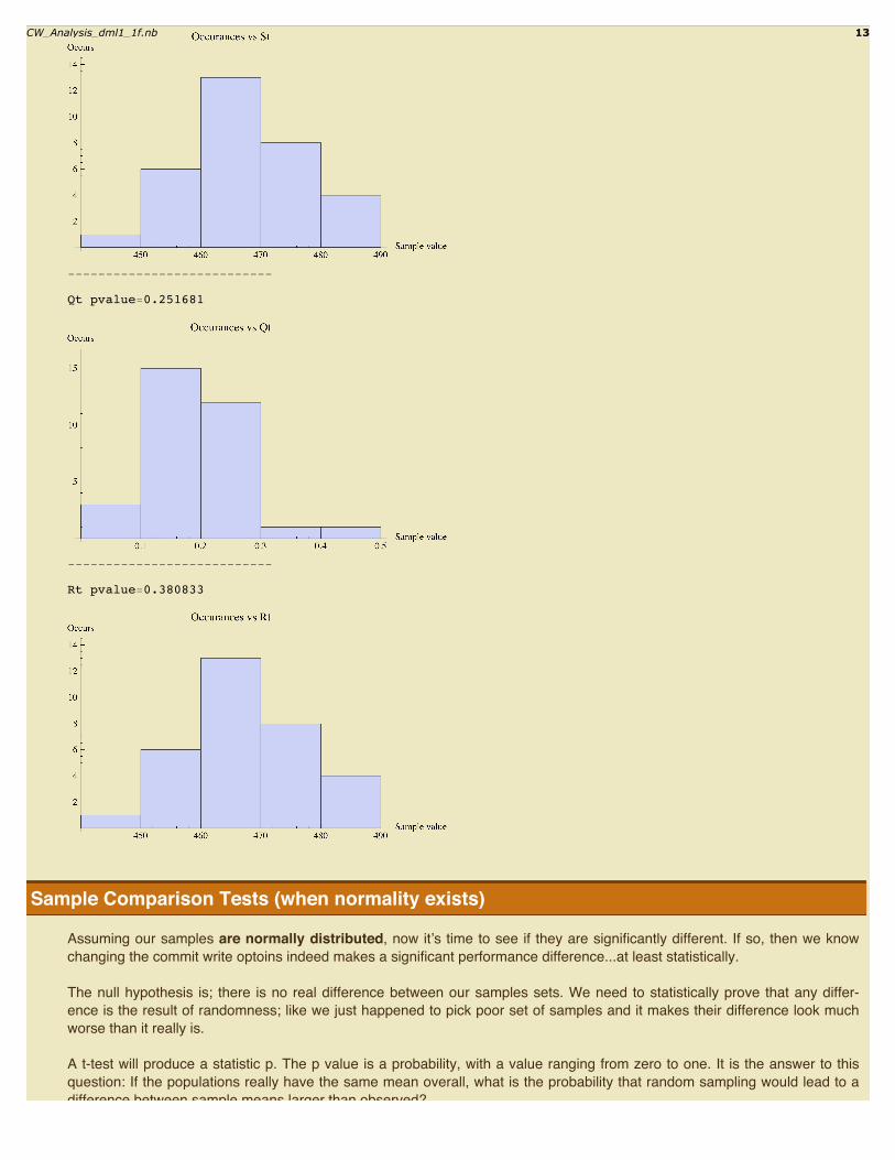
Wait BatchH32L and Nowait Immediate H32L
Work: 0.831121
L: 0.784703
St: 0.929672
Qt: 5.28216 µ 10-35
Rt: 6.18455 µ 10-13
==============================================================
Wait BatchH32L and Nowait Batch H32L
Work: 0.868893
L: 0.81588
St: 0.511946
Qt: 3.6158 µ 10-44
Rt: 1.92621 µ 10-13
==============================================================
Nowait ImmediateH32L and Wait Immediate H32L
Work: 0.00980034
L: 0.00938465
St: 0.0692285
CW_Analysis_dml1_1f.nb 15
Qt: 1.21047 µ 10-39
Rt: 1.95955 µ 10-15
==============================================================
Nowait ImmediateH32L and Wait Batch H32L
Work: 0.831121
L: 0.784703
St: 0.929672
Qt: 5.28216 µ 10-35
Rt: 6.18455 µ 10-13
==============================================================
Nowait ImmediateH32L and Nowait Batch H32L
Work: 0.944143
L: 0.944292
St: 0.476899
Qt: 0.0502241
Rt: 0.741235
==============================================================
Nowait BatchH32L and Wait Immediate H32L
Work: 0.00481099
L: 0.00458214
St: 0.194013
Qt: 1.45446 µ 10-38
Rt: 5.38924 µ 10-16
==============================================================
Nowait BatchH32L and Wait Batch H32L
Work: 0.868893
L: 0.81588
St: 0.511946
Qt: 3.6158 µ 10-44
Rt: 1.92621 µ 10-13
==============================================================
Nowait BatchH32L and Nowait Immediate H32L
Work: 0.944143
L: 0.944292
St: 0.476899
Qt: 0.0502241
Rt: 0.741235
If the above T-Test results (p value) are less then our threshold we can say there is a significant difference between the twosample sets.
Sample Comparison Tests (when normality may NOT exist)
If our sample sets are not normally distributed, we can not perform a simple t-test. We can perform what are called loca-tion tests. I did some research on significance testing when non-normal distributions exists. I found a very nice reference:
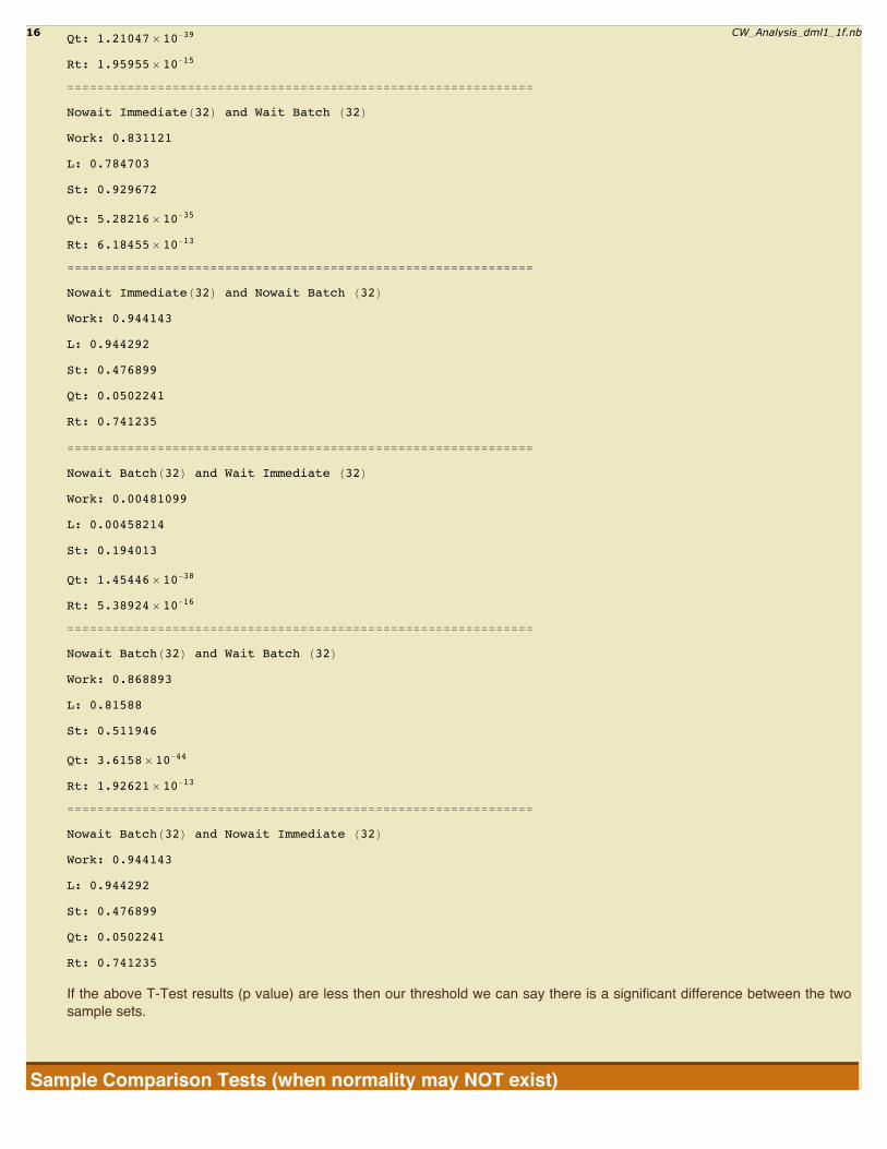
http://www.statsoft.com/textbook/nonparametric-statistics
The paragraph below (which is from the reference above) is a key reference to what we’re doing here:
...the need is evident for statistical procedures that enable us to process data of “low quality,” from small samples, on vari-ables about which nothing is known (concerning their distribution). Specifically, nonparametric methods were developed tobe used in cases when the researcher knows nothing about the parameters of the variable of interest in the population(hence the name nonparametric). In more technical terms, nonparametric methods do not rely on the estimation of parame-ters (such as the mean or the standard deviation) describing the distribution of the variable of interest in the population.Therefore, these methods are also sometimes (and more appropriately) called parameter-free methods or distribution-freemethods.
Being that I’m not a statistician but still need to determine if these sample sets are significant different, I let Mathematicadetermine the appropriate test. Notice that one of the above mentioned tests will probably be the test Mathematica chooses.
Note: If we run our normally distributed data through this analysis (speically, the “LocationEquivalenceTest”), Mathematicashould detect this and use a more appropriate significant test, like a t-test.Here we go with the hypothesis testing (assuming our sample sets are not normally distributed):
1. Our P value threshold is 0.05, which is our alpha.2. The null hypotheses is the two populations have the same mean. (Remember we have to sample sets, which is not thepopulation.)3. Do the statistical test to compute the P value.4. Compare the result P value to our threshold alpha value. If the P value is less then our threshold, we will reject the nullhypothesis and say the difference between our samples is significant. (Which is what I’m hoping to see.) However, if the Pvalue is greater than the threshold, we cannot reject the null hypothesis and any difference between our samples are notstatistically significant; randomness, picked the “wrong” samples, etc.
16 CW_Analysis_dml1_1f.nb
If our sample sets are not normally distributed, we can not perform a simple t-test. We can perform what are called loca-tion tests. I did some research on significance testing when non-normal distributions exists. I found a very nice reference:
http://www.statsoft.com/textbook/nonparametric-statistics
The paragraph below (which is from the reference above) is a key reference to what we’re doing here:
...the need is evident for statistical procedures that enable us to process data of “low quality,” from small samples, on vari-ables about which nothing is known (concerning their distribution). Specifically, nonparametric methods were developed tobe used in cases when the researcher knows nothing about the parameters of the variable of interest in the population(hence the name nonparametric). In more technical terms, nonparametric methods do not rely on the estimation of parame-ters (such as the mean or the standard deviation) describing the distribution of the variable of interest in the population.Therefore, these methods are also sometimes (and more appropriately) called parameter-free methods or distribution-freemethods.
Being that I’m not a statistician but still need to determine if these sample sets are significant different, I let Mathematicadetermine the appropriate test. Notice that one of the above mentioned tests will probably be the test Mathematica chooses.
Note: If we run our normally distributed data through this analysis (speically, the “LocationEquivalenceTest”), Mathematicashould detect this and use a more appropriate significant test, like a t-test.Here we go with the hypothesis testing (assuming our sample sets are not normally distributed):
1. Our P value threshold is 0.05, which is our alpha.2. The null hypotheses is the two populations have the same mean. (Remember we have to sample sets, which is not thepopulation.)3. Do the statistical test to compute the P value.4. Compare the result P value to our threshold alpha value. If the P value is less then our threshold, we will reject the nullhypothesis and say the difference between our samples is significant. (Which is what I’m hoping to see.) However, if the Pvalue is greater than the threshold, we cannot reject the null hypothesis and any difference between our samples are notstatistically significant; randomness, picked the “wrong” samples, etc.
CW_Analysis_dml1_1f.nb 17

Print@"P-values assumming normality MAY not exist."D;Table@
Table@If@i ¹≠ j,
Print@"=============================================================="D;Print@ssName@iD, "H", Length@ssL@iDD, "L and ", ssName@jD, " H", Length@ssL@jDD, "L"D;
test1 = MannWhitneyTest@8ssWork@iD, ssWork@jD<D;test2 = LocationEquivalenceTest@8ssWork@iD, ssWork@jD<, 8"TestDataTable", "AutomaticTest"<D;Print@"Work: Test1=", test1, " Test2=", test2D;Print@SmoothHistogram@8ssWork@iD, ssWork@jD<DD;
Print@"------------"D;test1 = MannWhitneyTest@8ssL@iD, ssL@jD<D;test2 = LocationEquivalenceTest@8ssL@iD, ssL@jD<, 8"TestDataTable", "AutomaticTest"<D;Print@"L: Test1=", test1, " Test2=", test2D;Print@SmoothHistogram@8ssL@iD, ssL@jD<DD;
Print@"------------"D;test1 = MannWhitneyTest@8ssSt@iD, ssSt@jD<D;test2 = LocationEquivalenceTest@8ssSt@iD, ssSt@jD<, 8"TestDataTable", "AutomaticTest"<D;Print@"St: Test1=", test1, " Test2=", test2D;Print@SmoothHistogram@8ssSt@iD, ssSt@jD<DD;
Print@"------------"D;test1 = MannWhitneyTest@8ssQt@iD, ssQt@jD<D;test2 = LocationEquivalenceTest@8ssQt@iD, ssQt@jD<, 8"TestDataTable", "AutomaticTest"<D;Print@"Qt: Test1=", test1, " Test2=", test2D;Print@SmoothHistogram@8ssQt@iD, ssQt@jD<DD;
Print@"------------"D;test1 = MannWhitneyTest@8ssRt@iD, ssRt@jD<D;test2 = LocationEquivalenceTest@8ssRt@iD, ssRt@jD<, 8"TestDataTable", "AutomaticTest"<D;Print@"St: Test1=", test1, " Test2=", test2D;Print@SmoothHistogram@8ssRt@iD, ssRt@jD<DD;
D;,8j, 1, ssNum<
D;, 8i, 1, ssNum<
D;
P-values assumming normality MAY not exist.
==============================================================
Wait ImmediateH32L and Wait Batch H32L
Work: Test1=0.0180978 Test2=: Statistic P-ValueK-Sample T 6.8993 0.0108505
, KSampleT>
700 750 800
0.005
0.010
0.015
------------
L: Test1=0.0191274 Test2=: Statistic P-ValueK-Sample T 6.70476 0.0119672
, KSampleT>
18 CW_Analysis_dml1_1f.nb

0.0080 0.0085 0.0090
500
1000
1500
------------
St: Test1=0.130902 Test2=: Statistic P-ValueK-Sample T 3.42364 0.0690354
, KSampleT>
460 480 500 520
0.01
0.02
0.03
------------
Qt: Test1=0.386462 Test2=: Statistic P-ValueKruskal-Wallis 0.761719 0.387064
, KruskalWallis>
22 25 28 30 32
0.1
0.2
0.3
------------
St: Test1=0.114637 Test2=: Statistic P-ValueK-Sample T 3.85155 0.0541915
, KSampleT>
CW_Analysis_dml1_1f.nb 19

480 500 520 540
0.01
0.02
0.03
==============================================================
Wait ImmediateH32L and Nowait Immediate H32L
Work: Test1=0.0236441 Test2=: Statistic P-ValueKruskal-Wallis 5.09219 0.0227979
, KruskalWallis>
750 800
0.005
0.010
0.015
0.020
0.025
------------
L: Test1=0.0253766 Test2=: Statistic P-ValueKruskal-Wallis 4.96803 0.0245961
, KruskalWallis>
0.0080 0.0085 0.0090
500
1000
1500
2000
------------
St: Test1=0.172928 Test2=: Statistic P-ValueK-Sample T 3.41876 0.0692285
, KSampleT>
20 CW_Analysis_dml1_1f.nb

440 460 480 500 520
0.01
0.02
0.03
------------
Qt: Test1=6.51131 µ 10-12 Test2=: Statistic P-ValueKruskal-Wallis 47.2615 2.45726µ10-20 , KruskalWallis>
10 20 30
0.50
1.00
1.50
2.00
2.50
------------
St: Test1=7.08328 µ 10-11 Test2=:Statistic P-Value
K-Sample T 110.862 1.95955µ10-15 , KSampleT>
425 450 475 500 525
0.01
0.02
0.03
==============================================================
Wait ImmediateH32L and Nowait Batch H32L
Work: Test1=0.00388399 Test2=: Statistic P-ValueK-Sample T 8.55364 0.00481099
, KSampleT>
CW_Analysis_dml1_1f.nb 21

675 700 725 750 775 800
0.005
0.010
0.015
0.020
------------
L: Test1=0.00349576 Test2=: Statistic P-ValueK-Sample T 8.65493 0.00458214
, KSampleT>
0.0075 0.0080 0.0085 0.0090
500
1000
1500
2000
------------
St: Test1=0.273818 Test2=: Statistic P-ValueK-Sample T 1.72404 0.194013
, KSampleT>
460 480 500 520
0.01
0.02
0.03
------------
Qt: Test1=6.50414 µ 10-12 Test2=:Statistic P-Value
K-Sample T 7370.44 3.67139µ10-66 , KSampleT>
22 CW_Analysis_dml1_1f.nb
10 20 30
1
2
3
4
------------
St: Test1=7.08328 µ 10-11 Test2=:Statistic P-Value
K-Sample T 118.151 5.38924µ10-16 , KSampleT>
460 480 500 520 540
0.01
0.02
0.03
==============================================================
Wait BatchH32L and Wait Immediate H32L
Work: Test1=0.0187642 Test2=: Statistic P-ValueK-Sample T 6.8993 0.0108505
, KSampleT>
700 750 800
0.005
0.010
0.015
------------
L: Test1=0.0198267 Test2=: Statistic P-ValueK-Sample T 6.70476 0.0119672
, KSampleT>
CW_Analysis_dml1_1f.nb 23

0.0080 0.0085 0.0090
500
1000
1500
------------
St: Test1=0.127513 Test2=: Statistic P-ValueK-Sample T 3.42364 0.0690354
, KSampleT>
460 480 500 520
0.01
0.02
0.03
------------
Qt: Test1=0.379142 Test2=: Statistic P-ValueKruskal-Wallis 0.761719 0.387064
, KruskalWallis>
22 25 28 30 32
0.1
0.2
0.3
------------
St: Test1=0.111583 Test2=: Statistic P-ValueK-Sample T 3.85155 0.0541915
, KSampleT>
24 CW_Analysis_dml1_1f.nb
480 500 520 540
0.01
0.02
0.03
==============================================================
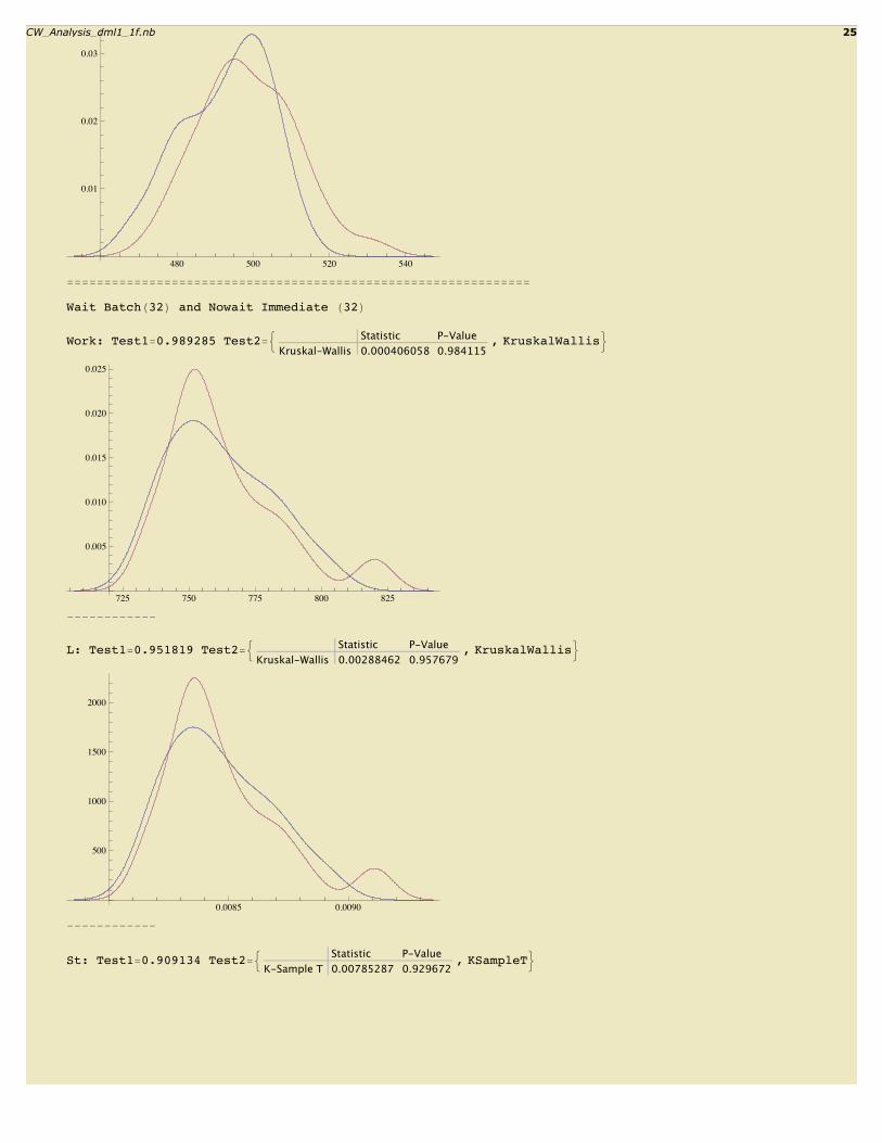
Wait BatchH32L and Nowait Immediate H32L
Work: Test1=0.989285 Test2=: Statistic P-ValueKruskal-Wallis 0.000406058 0.984115
, KruskalWallis>
725 750 775 800 825
0.005
0.010
0.015
0.020
0.025
------------
L: Test1=0.951819 Test2=: Statistic P-ValueKruskal-Wallis 0.00288462 0.957679
, KruskalWallis>
0.0085 0.0090
500
1000
1500
2000
------------
St: Test1=0.909134 Test2=: Statistic P-ValueK-Sample T 0.00785287 0.929672
, KSampleT>
CW_Analysis_dml1_1f.nb 25

440 460 480 500
0.01
0.02
0.03
------------
Qt: Test1=6.51131 µ 10-12 Test2=: Statistic P-ValueKruskal-Wallis 47.2615 2.45726µ10-20 , KruskalWallis>
10 20 30
0.50
1.00
1.50
2.00
2.50
------------
St: Test1=6.83863 µ 10-10 Test2=:Statistic P-Value
K-Sample T 81.8401 6.18455µ10-13 , KSampleT>
440 460 480 500 520
0.01
0.02
0.03
==============================================================
Wait BatchH32L and Nowait Batch H32L
Work: Test1=0.609815 Test2=: Statistic P-ValueK-Sample T 0.0274729 0.868893
, KSampleT>
26 CW_Analysis_dml1_1f.nb

725 750 775 800 825
0.005
0.010
0.015
0.020
------------
L: Test1=0.568234 Test2=: Statistic P-ValueK-Sample T 0.0546811 0.81588
, KSampleT>
0.0080 0.0083 0.0085 0.0088 0.0090
500
1000
1500
2000
------------
St: Test1=0.6146 Test2=: Statistic P-ValueK-Sample T 0.435088 0.511946
, KSampleT>
440 460 480 500
0.01
0.02
0.03
------------
Qt: Test1=6.50414 µ 10-12 Test2=: Statistic P-ValueKruskal-Wallis 47.2615 2.45726µ10-20 , KruskalWallis>
CW_Analysis_dml1_1f.nb 27

10 20 30
1
2
3
4
------------
St: Test1=9.59121 µ 10-10 Test2=:Statistic P-Value
K-Sample T 87.2935 1.92621µ10-13 , KSampleT>
460 480 500 520
0.01
0.02
0.03
==============================================================
Nowait ImmediateH32L and Wait Immediate H32L
Work: Test1=0.0244849 Test2=: Statistic P-ValueKruskal-Wallis 5.09219 0.0227979
, KruskalWallis>
750 800
0.005
0.010
0.015
0.020
0.025
------------
L: Test1=0.0262702 Test2=: Statistic P-ValueKruskal-Wallis 4.96803 0.0245961
, KruskalWallis>
28 CW_Analysis_dml1_1f.nb

0.0080 0.0085 0.0090
500
1000
1500
2000
------------
St: Test1=0.168734 Test2=: Statistic P-ValueK-Sample T 3.41876 0.0692285
, KSampleT>
440 460 480 500 520
0.01
0.02
0.03
------------
Qt: Test1=5.92604 µ 10-12 Test2=: Statistic P-ValueKruskal-Wallis 47.2615 2.45726µ10-20 , KruskalWallis>
10 20 30
0.50
1.00
1.50
2.00
2.50
------------
St: Test1=6.47628 µ 10-11 Test2=:Statistic P-Value
K-Sample T 110.862 1.95955µ10-15 , KSampleT>
CW_Analysis_dml1_1f.nb 29

425 450 475 500 525
0.01
0.02
0.03
==============================================================
Nowait ImmediateH32L and Wait Batch H32L
Work: Test1=0.978572 Test2=: Statistic P-ValueKruskal-Wallis 0.000406058 0.984115
, KruskalWallis>
725 750 775 800 825
0.005
0.010
0.015
0.020
0.025
------------
L: Test1=0.962517 Test2=: Statistic P-ValueKruskal-Wallis 0.00288462 0.957679
, KruskalWallis>
0.0085 0.0090
500
1000
1500
2000
------------
St: Test1=0.898499 Test2=: Statistic P-ValueK-Sample T 0.00785287 0.929672
, KSampleT>
30 CW_Analysis_dml1_1f.nb
440 460 480 500
0.01
0.02
0.03
------------
Qt: Test1=5.92604 µ 10-12 Test2=: Statistic P-ValueKruskal-Wallis 47.2615 2.45726µ10-20 , KruskalWallis>
10 20 30
0.50
1.00
1.50
2.00
2.50
------------
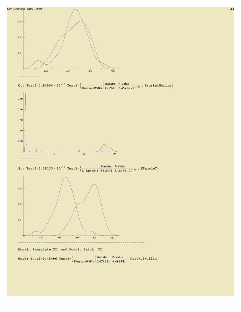
St: Test1=6.28133 µ 10-10 Test2=:Statistic P-Value
K-Sample T 81.8401 6.18455µ10-13 , KSampleT>
440 460 480 500 520
0.01
0.02
0.03
==============================================================
Nowait ImmediateH32L and Nowait Batch H32L
Work: Test1=0.48496 Test2=: Statistic P-ValueKruskal-Wallis 0.478521 0.493481
, KruskalWallis>
CW_Analysis_dml1_1f.nb 31

725 750 775 800 825
0.005
0.010
0.015
0.020
0.025
------------
L: Test1=0.497727 Test2=: Statistic P-ValueKruskal-Wallis 0.450721 0.506357
, KruskalWallis>
0.0080 0.0085 0.0090
500
1000
1500
2000
------------
St: Test1=0.803823 Test2=: Statistic P-ValueK-Sample T 0.512142 0.476899
, KSampleT>
440 460 480 500
0.01
0.02
0.03
------------
Qt: Test1=7.84824 µ 10-12 Test2=: Statistic P-ValueKruskal-Wallis 46.893 5.05453µ10-20 , KruskalWallis>
32 CW_Analysis_dml1_1f.nb

5 10 15
1
2
3
4
------------
St: Test1=0.973222 Test2=: Statistic P-ValueK-Sample T 0.110024 0.741235
, KSampleT>
440 460 480 500
0.01
0.02
0.03
==============================================================
Nowait BatchH32L and Wait Immediate H32L
Work: Test1=0.00405305 Test2=: Statistic P-ValueK-Sample T 8.55364 0.00481099
, KSampleT>
675 700 725 750 775 800
0.005
0.010
0.015
0.020
------------
L: Test1=0.00364938 Test2=: Statistic P-ValueK-Sample T 8.65493 0.00458214
, KSampleT>
CW_Analysis_dml1_1f.nb 33

0.0075 0.0080 0.0085 0.0090
500
1000
1500
2000
------------
St: Test1=0.267974 Test2=: Statistic P-ValueK-Sample T 1.72404 0.194013
, KSampleT>
460 480 500 520
0.01
0.02
0.03
------------
Qt: Test1=5.91948 µ 10-12 Test2=:Statistic P-Value
K-Sample T 7370.44 3.67139µ10-66 , KSampleT>
10 20 30
1
2
3
4
------------
St: Test1=6.47628 µ 10-11 Test2=:Statistic P-Value
K-Sample T 118.151 5.38924µ10-16 , KSampleT>
34 CW_Analysis_dml1_1f.nb

460 480 500 520 540
0.01
0.02
0.03
==============================================================
Nowait BatchH32L and Wait Batch H32L
Work: Test1=0.619255 Test2=: Statistic P-ValueK-Sample T 0.0274729 0.868893
, KSampleT>
725 750 775 800 825
0.005
0.010
0.015
0.020
------------
L: Test1=0.577372 Test2=: Statistic P-ValueK-Sample T 0.0546811 0.81588
, KSampleT>
0.0080 0.0083 0.0085 0.0088 0.0090
500
1000
1500
2000
------------
St: Test1=0.624069 Test2=: Statistic P-ValueK-Sample T 0.435088 0.511946
, KSampleT>
CW_Analysis_dml1_1f.nb 35

440 460 480 500
0.01
0.02
0.03
------------
Qt: Test1=5.91948 µ 10-12 Test2=: Statistic P-ValueKruskal-Wallis 47.2615 2.45726µ10-20 , KruskalWallis>
10 20 30
1
2
3
4
------------
St: Test1=8.8158 µ 10-10 Test2=:Statistic P-Value
K-Sample T 87.2935 1.92621µ10-13 , KSampleT>
460 480 500 520
0.01
0.02
0.03
==============================================================
Nowait BatchH32L and Nowait Immediate H32L
Work: Test1=0.493396 Test2=: Statistic P-ValueKruskal-Wallis 0.478521 0.493481
, KruskalWallis>
36 CW_Analysis_dml1_1f.nb

725 750 775 800 825
0.005
0.010
0.015
0.020
0.025
------------
L: Test1=0.506278 Test2=: Statistic P-ValueKruskal-Wallis 0.450721 0.506357
, KruskalWallis>
0.0080 0.0085 0.0090
500
1000
1500
2000
------------
St: Test1=0.814228 Test2=: Statistic P-ValueK-Sample T 0.512142 0.476899
, KSampleT>
440 460 480 500
0.01
0.02
0.03
------------
Qt: Test1=7.14528 µ 10-12 Test2=: Statistic P-ValueKruskal-Wallis 46.893 5.05453µ10-20 , KruskalWallis>
CW_Analysis_dml1_1f.nb 37

5 10 15
1
2
3
4
------------
St: Test1=0.962517 Test2=: Statistic P-ValueK-Sample T 0.110024 0.741235
, KSampleT>
440 460 480 500
0.01
0.02
0.03
Visually Comparing All Samples
I also wanted to get a nice visual picture of my sample sets...together. Sometimes I include all the sample sets and some-times I don’t. It’s just based on what I want to convey. Sometimes you get a more appropriate view if all the data is notincluded.
Here is the colors in order of sample set; blue, red, yellow, green.
38 CW_Analysis_dml1_1f.nb

gset = 8<;Table@
AppendTo@gset, ssWork@iDD;, 8i, 1, ssNum<
D;SmoothHistogram@gset,PlotLabel Ø "Occurances vs Work HcmtL", AxesLabel Ø 8"cmt", "Occurs"<D
750 800cmt
0.005
0.010
0.015
0.020
0.025Occurs
Occurances vs Work HcmtL
gset = 8<;Table@
AppendTo@gset, ssL@iDD;, 8i, 1, ssNum<
D;SmoothHistogram@gset,PlotLabel Ø "Occurances vs Workload HcmtêmsL", AxesLabel Ø 8"cmtêworkload", "Occurs"<D
0.0080 0.0085 0.0090cmtêworkload
500
1000
1500
2000
OccursOccurances vs Workload HcmtêmsL
CW_Analysis_dml1_1f.nb 39

gset = 8<;Table@
AppendTo@gset, ssSt@iDD;, 8i, 1, ssNum<
D;SmoothHistogram@gset,PlotLabel Ø "Occurances vs CPUHmsLêcmt", AxesLabel Ø 8"CPUHmsLêcmt", "Occurs"<D
440 460 480 500 520CPUHmsLêcmt
0.01
0.02
0.03
OccursOccurances vs CPUHmsLêcmt
gset = 8<;Table@
AppendTo@gset, ssQt@iDD;, 8i, 1, ssNum<
D;SmoothHistogram@gset,PlotLabel Ø "Occurances vs WaitHmsLêcmt", AxesLabel Ø 8"WaitHmsLêcmt", "Occurs"<D
10 20 30WaitHmsLêcmt
1
2
3
4
OccursOccurances vs WaitHmsLêcmt
40 CW_Analysis_dml1_1f.nb

gset = 8<;Table@
AppendTo@gset, ssRt@iDD;, 8i, 1, ssNum<
D;SmoothHistogram@gset,PlotLabel Ø "Occurances vs CPU+WaitHmsLêcmt", AxesLabel Ø 8"CPU+WaitHmsLêcmt", "Occurs"<D
425 450 475 500 525CPU+WaitHmsLêcmt
0.01
0.02
0.03
OccursOccurances vs CPU+WaitHmsLêcmt
Fair: Comparing situations fairly
As workload increases, we can expect response time to also increase. If the workload is decreases response time maydecrease. When comparing two sample sets, if their arrival rates are different, comparing their queue times and responsetimes using statitcal significant tests is problematic and downright unfiar.
To get around this problem, we need to do the testing at the same arrival rate. However, our sample data may not have beencollected at the same arrival rate! That’s a problem.
To get this problem, we need to develop an equation for each of our four sample sets relating the arrival rate to the responsetime. Fortunately, there already exists a formal mathematical equation related the arrival rate, service time, queue time, thenumber of transaction processors (think: CPU cores), and the response time.
For a CPU constained system, the equation is r = s / (1-(sL/m)^m)
For an IO constrained system, the equation is r = s / (1-(sL/m))
There are many ways to go about this process. Here is who I’m choosing to do it. Within in each of the four sample sets(ssNum), for each sample value (sampleIdx), I derive the missing variable M and store these in mList. Then I take the aver-age M and save that in bestMList. I could have weighted the average or taken the median, but I just kept it simple. You seethe details in the code segment below.
Note that this can take awhile to run. The “Solve” is cpu intensive.
CW_Analysis_dml1_1f.nb 41
Clear@s, q, r, l, sol, bestM, mList, bestMListD;bestMList = 8<;Table@
mList = 8<;Table@s = ssSt@ssidxD@@sampleIdxDD;q = ssQt@ssidxD@@sampleIdxDD;r = s + q;l = ssL@ssidxD@@sampleIdxDD;sol = Solve@s ê H1 - Hs * l ê mL^mL ã r && m > 0, mD;8mm< = m ê. sol;H*Print@ssidx," ",sampleIdx," mm=",mmD;*LAppendTo@mList, mmD;, 8sampleIdx, 1, sampleNum<
D;bestM = Mean@mListD;H*Print@ssidx," bestM=",bestMD;*LAppendTo@bestMList, bestMD;, 8ssidx, 1, ssNum<
D;
Solve::ratnz : Solve was unable to solve the system with inexact coefficients.The answer was obtained by solving a corresponding exact system and numericizing the result. à
Solve::ratnz : Solve was unable to solve the system with inexact coefficients.The answer was obtained by solving a corresponding exact system and numericizing the result. à
Solve::ratnz : Solve was unable to solve the system with inexact coefficients.The answer was obtained by solving a corresponding exact system and numericizing the result. à
General::stop : Further output of Solve::ratnz will be suppressed during this calculation. à
Print@"The best M values are:"D;Table@
Print@ssName@ssidxD, " M=", bestMList@@ssidxDDD;, 8ssidx, 1, ssNum<
D;
The best M values are:
Wait Immediate M=6.23085
Wait Batch M=6.25177
Nowait Immediate M=8.41341
Nowait Batch M=9.24755
The baseline arrival rate will be the average from our first sample set, (nowait, immediate). I expect the other three options toprovide better performance and the nowwait,immediate is the Oracle default, hence this is my chosen baseline.
baselineL = Mean@ssL@1DD
0.00831995
Now that we have a good M for each of our four sample sets (bestMList) along with the standard arrival rate (baselineL), andthe observed service time for each individual sample, we will derive the queue time and the response time for each indivisualsample (within each of our four sample sets). All the inputs and derived queue time and response time are stored in thestandardized lists, stndL, stndM, stndSt, stndQt, and stndRt. At this point, we essentially have an entirely new (i.e., standard-ized) set of experimental data. This allows us to run this data through the same statistical analysis as I did above!
42 CW_Analysis_dml1_1f.nb

Clear@stndRt, stndSt, stndL, stndQt, stndMD;Clear@s, l, m, r, qD;Table@
stndRt@ssidxD = 8<;stndQt@ssidxD = 8<;stndSt@ssidxD = 8<;stndL@ssidxD = 8<;stndM@ssidxD = 8<;Table@s = ssSt@ssidxD@@sampleIdxDD;l = baselineL;m = bestMList@@ssidxDD;r = s ê H1 - Hs l ê mL^mL;q = r - s;H*Print@ssidx," ",sampleIdx," s=",s," l=",l," m=",m," r=",rD;*LAppendTo@stndRt@ssidxD, rD;AppendTo@stndSt@ssidxD, sD;AppendTo@stndL@ssidxD, lD;AppendTo@stndQt@ssidxD, qD;AppendTo@stndM@ssidxD, mD;, 8sampleIdx, 1, sampleNum<
D;, 8ssidx, 1, ssNum<
D;stndM@1DstndL@1DstndSt@1DstndQt@1DstndRt@1D
86.23085, 6.23085, 6.23085, 6.23085, 6.23085, 6.23085, 6.23085, 6.23085, 6.23085, 6.23085, 6.23085,6.23085, 6.23085, 6.23085, 6.23085, 6.23085, 6.23085, 6.23085, 6.23085, 6.23085, 6.23085, 6.23085,6.23085, 6.23085, 6.23085, 6.23085, 6.23085, 6.23085, 6.23085, 6.23085, 6.23085, 6.23085<
80.00831995, 0.00831995, 0.00831995, 0.00831995, 0.00831995, 0.00831995, 0.00831995, 0.00831995,0.00831995, 0.00831995, 0.00831995, 0.00831995, 0.00831995, 0.00831995, 0.00831995, 0.00831995,0.00831995, 0.00831995, 0.00831995, 0.00831995, 0.00831995, 0.00831995, 0.00831995, 0.00831995,0.00831995, 0.00831995, 0.00831995, 0.00831995, 0.00831995, 0.00831995, 0.00831995, 0.00831995<
8459.616, 473.553, 453.723, 461.943, 479.949, 467.896, 504.242, 465.825, 473.903, 479.533, 463.854,463.434, 483.655, 458.153, 466.594, 482.754, 481.4, 472.362, 468.953, 480.046, 477.321, 490.003,459.735, 463.804, 457.969, 450.973, 472.195, 479.738, 491.073, 467.791, 471.59, 447.642<
823.0411, 28.8926, 20.9072, 23.9363, 32.0062, 26.3718, 46.8654, 25.5002, 29.0554, 31.7948, 24.6948,24.5264, 33.9481, 22.4937, 25.8205, 33.4663, 32.7542, 28.3444, 26.8269, 32.0555, 30.6917,37.5278, 23.086, 24.6748, 22.4256, 19.9741, 28.268, 31.8989, 38.1643, 26.3272, 27.9941, 18.8936<
8482.657, 502.445, 474.63, 485.879, 511.955, 494.268, 551.107, 491.325, 502.958, 511.328, 488.548,487.961, 517.603, 480.647, 492.414, 516.22, 514.155, 500.706, 495.779, 512.101, 508.013, 527.531,482.821, 488.479, 480.394, 470.948, 500.463, 511.637, 529.238, 494.119, 499.584, 466.536<
Fair: Basic Statistics
Using our standardized data, in this section I calculate the basic statistics, such as the mean and median. My objective is toensure the data has been collected and entered correctly and also to compare the two datasets to see if they appear to bedifferent.
CW_Analysis_dml1_1f.nb 43

myData = Table@8ssName@ssidxD, Mean@stndL@ssidxDD, Mean@stndSt@ssidxDD,Mean@stndQt@ssidxDD, Mean@stndRt@ssidxDD, Length@stndL@ssidxDD,N@StandardDeviation@stndL@ssidxDDD, N@StandardDeviation@stndSt@ssidxDDD,N@StandardDeviation@stndQt@ssidxDDD, N@StandardDeviation@stndRt@ssidxDDD
<, 8ssidx, 1, ssNum<D;
toGrid = Prepend@myData, 8"Settings", "Avg L\nHcmtêmsL", "Avg CPUt\nHmsêcmtL","Avg Wt\nHmsêcmtL", "Avg Rt\nHmsêcmtL", "Samples", "Stdev L\nHcmtêmsL","Stdev CPUt\nHmsêcmtL", "Stdev Wt\nHmsêcmtL", "Stdev Rt\nHmsêcmtL"<D;
Grid@toGrid,Frame ØAllD
Settings Avg LHcmtêms
L
Avg CPUtHmsêcmtL
Avg WtHmsêcmtL
Avg RtHmsêcmtL
Samples Stdev LHcmtêmsL
StdevCPUt
HmsêcmtL
Stdev WtHmsêcmtL
Stdev RtHmsêcmtL
WaitImmediÖate
0.008319Ö95
470.976 28.2259 499.202 32 1.76248 µ
10-1812.4358 5.9129 18.3156
WaitBatch
0.008319Ö95
465.452 24.9021 490.354 32 1.76248 µ
10-1811.4239 4.49972 15.9122
NowaitImmediÖate
0.008319Ö95
465.186 0.696187 465.882 32 1.76248 µ
10-1812.6153 0.166351 12.7791
NowaitBatch
0.008319Ö95
467.24 0.158056 467.398 32 1.76248 µ
10-1810.2195 0.0359533 10.2553
Using our standardized data, in this section I calculate the key parameters for understanding the impact or change of thesettings.
myData = Table@8ssName@ssidxD,Mean@stndL@ssidxDD, 100 * HMean@stndL@ssidxDD - Mean@stndL@1DDL ê Mean@stndL@1DD,Mean@stndSt@ssidxDD, 100 * HMean@stndSt@ssidxDD - Mean@stndSt@1DDL ê Mean@stndSt@1DD,Mean@stndQt@ssidxDD, 100 * HMean@stndQt@ssidxDD - Mean@stndQt@1DDL ê Mean@stndQt@1DD,Mean@stndRt@ssidxDD, 100 * HMean@stndRt@ssidxDD - Mean@stndRt@1DDL ê Mean@stndRt@1DD,Length@stndL@ssidxDD
<, 8ssidx, 1, ssNum<D;
toGrid = Prepend@myData, 8"Settings", "Avg L\nHcmtêmsL", "%\nChange", "Avg CPUt\nHmsêcmtL","%\nChange", "Avg Wt\nHmsêcmtL", "%\nChange", "Avg Rt\nHmsêcmtL", "%\nChange", "Samples"<D;
Grid@toGrid,Frame ØAllD
Settings Avg LHcmtêmsL
%Change
Avg CPUtHmsêcmtL
%Change
Avg WtHmsêcmtL
%Change
Avg RtHmsêcmtL
%Change
Samples
Wait Immediate 0.00831995 0. 470.976 0. 28.2259 0. 499.202 0. 32Wait Batch 0.00831995 0. 465.452 -1.17276 24.9021 -11.7758 490.354 -1.77228 32Nowait
Immediate0.00831995 0. 465.186 -1.22937 0.696187 -97.5335 465.882 -6.6746 32
Nowait Batch 0.00831995 0. 467.24 -0.793276 0.158056 -99.44 467.398 -6.37096 32
44 CW_Analysis_dml1_1f.nb


![INDEX [ptgmedia.pearsoncmg.com] · 2009. 6. 9. · two-phase commit protocol, 369 Web services transactions, support for, 371 Commit, 7 two-phase, 7–8 Commit check, 132 Commit command,](https://img.pdfslide.us/doc/110x75/5fe1ed01a48cc3790b473c6a/index-2009-6-9-two-phase-commit-protocol-369-web-services-transactions.jpg)