Embed Size (px)
Citation preview

COMMISSIONING OF A REFRIGERANT TEST
UNIT AND ASSESSING THE PERFORMANCE
OF REFRIGERANT BLENDS
Ndlovu Phakamile
B. Eng. (Hons) NUST Zimbabwe
Submitted in fulfilment of the Academic Requirements for the Awards of the Master of
Science Degree in Engineering at the School of Chemical Engineering,
University of KwaZulu-Natal.
December 2017
Supervisor: Prof Paramespri Naidoo.
Co-supervisors: Prof Deresh Ramjugernath, Prof J.D Raal and Dr Caleb Narasigadu

i
As the candidate’s supervisor I agree to the submission of this thesis:
Prof. P. Naidoo Date
Declaration
I, Ndlovu Phakamile, student number 216074625 declare that:
(i) The research reported in this dissertation, except where otherwise indicated or
acknowledged, is my original work.
(ii) This dissertation has not been submitted in full or in part for any degree or examination
to any other university.
(iii) This dissertation does not contain other persons’ data, pictures, graphs or other
information unless specifically acknowledged as being sourced from other persons.
(iv) This dissertation does not contain other persons’ writing unless specifically
acknowledged as being sourced from other researchers. Where other written sources
have been quoted, then:
a) Their words have been rewritten but the general information attributed to them
has been referenced.
b) Where their exact words have been used, their writing has been placed inside
quotation marks, and referenced.
(v) This dissertation is primarily a collection of material, prepared by myself, published as
journal articles or presented as a poster and oral presentations at conferences. In some
cases, additional material has been included.
Signed: Date:
ii
Acknowledgements
I would like to thank God, the one “in whom we live and move and have our being” Acts 17 vs
28, who made it possible for me accomplish this feat. To my mother and father, thank you very
much for grooming a man in me. My brothers and sister, dreams do come true.
I would express my gratitude to my supervisors, Prof Deresh Ramjugernath, Prof Paramespri
Naidoo, Prof J.D Raal and Dr Caleb Narasigadu, for their invaluable knowledge they imparted,
their academic guidance and support throughout my study. My academic life has been
revolutionised because of learning from such academic giants.
I would like to thank Pelchem SOC, Fluorochemical Expansion Initiative and the NRF for
financial assistance, as well as the Thermodynamics Research Unit’s administrators, laboratory
technicians, and the department’s workshop technicians. Special thanks to A Khanyile for
taking time to assist me in the equipment handling.
To my friends and colleagues at Chemical Engineering, I am forever grateful for the friendship
and helpful criticism namely: Zibusiso L, Fredrick C, Obert M, Sandile N, Deliwe M,
Emmanuel G, Thandiwe M, Tauheedah A and Dr Samuel I.
Finally, to Alisha Shadrach, we have finally achieved what you set out to do. The refrigerant
unit is functioning perfectly, you did a great job in the design of the refrigerant unit.
iii
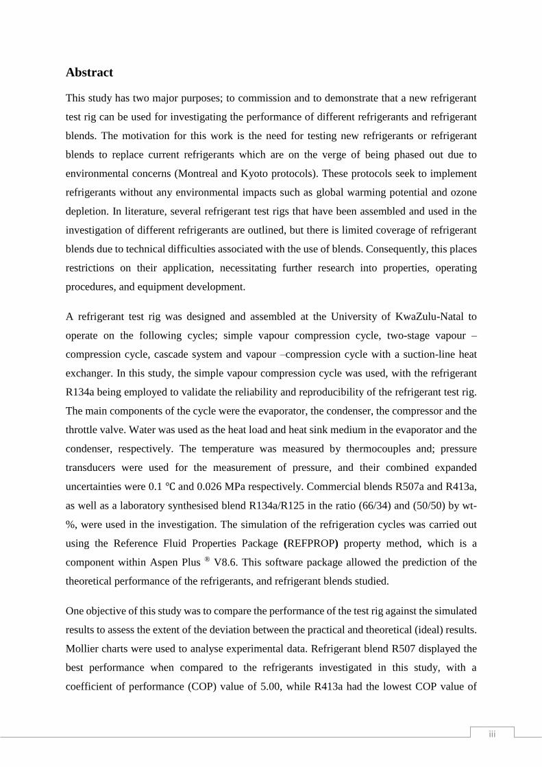
Abstract
This study has two major purposes; to commission and to demonstrate that a new refrigerant
test rig can be used for investigating the performance of different refrigerants and refrigerant
blends. The motivation for this work is the need for testing new refrigerants or refrigerant
blends to replace current refrigerants which are on the verge of being phased out due to
environmental concerns (Montreal and Kyoto protocols). These protocols seek to implement
refrigerants without any environmental impacts such as global warming potential and ozone
depletion. In literature, several refrigerant test rigs that have been assembled and used in the
investigation of different refrigerants are outlined, but there is limited coverage of refrigerant
blends due to technical difficulties associated with the use of blends. Consequently, this places
restrictions on their application, necessitating further research into properties, operating
procedures, and equipment development.
A refrigerant test rig was designed and assembled at the University of KwaZulu-Natal to
operate on the following cycles; simple vapour compression cycle, two-stage vapour –
compression cycle, cascade system and vapour –compression cycle with a suction-line heat
exchanger. In this study, the simple vapour compression cycle was used, with the refrigerant
R134a being employed to validate the reliability and reproducibility of the refrigerant test rig.
The main components of the cycle were the evaporator, the condenser, the compressor and the
throttle valve. Water was used as the heat load and heat sink medium in the evaporator and the
condenser, respectively. The temperature was measured by thermocouples and; pressure
transducers were used for the measurement of pressure, and their combined expanded
uncertainties were 0.1 ℃ and 0.026 MPa respectively. Commercial blends R507a and R413a,
as well as a laboratory synthesised blend R134a/R125 in the ratio (66/34) and (50/50) by wt-
%, were used in the investigation. The simulation of the refrigeration cycles was carried out
using the Reference Fluid Properties Package (REFPROP) property method, which is a
component within Aspen Plus ® V8.6. This software package allowed the prediction of the
theoretical performance of the refrigerants, and refrigerant blends studied.
One objective of this study was to compare the performance of the test rig against the simulated
results to assess the extent of the deviation between the practical and theoretical (ideal) results.
Mollier charts were used to analyse experimental data. Refrigerant blend R507 displayed the
best performance when compared to the refrigerants investigated in this study, with a
coefficient of performance (COP) value of 5.00, while R413a had the lowest COP value of

iv
4.00. Considering environmental aspects, R134a/R125 (66/34 wt %) with COP value of 4.88
has the least negative impact. The deviation between the theoretical and experimental values
was within the experimental uncertainty, with a notable difference occurring in the evaporator
inlet temperature. The results show that the test rig is fit for use in refrigeration experimental
work. Furthermore, refrigerant blends showed good performance on the vapour compression
cycles employed in this study proving that it is feasible to use the test rig in the investigation
of refrigerant blending.

v
Nomenclature
English letters
b. p boiling point
Cv flow coefficient
e specific exergy
E exergy
𝑓𝑥 Equivalent substance reducing ratios for the mixture
Fl pressure recovery factor
𝑔𝑧 Specific potential energy [J/kg]
ℎ Specific enthalpy [J/kg]
ℎ𝑥 Equivalent substance reducing ratios for the mixture
H Enthalpy
I exergy destruction rate [watts]
𝑘𝑖𝑗 Binary interaction parameter and are nonzero when 𝑖 ≠ 𝑗.
𝑙𝑖𝑗 Binary interaction parameter and are nonzero when 𝑖 ≠ 𝑗.
�� Mass flow rate of the refrigerant [kg/s]
MPa Mega Pascal
q Heat transfer per unit mass [J/kg]
�� Rate of heat transfer between the control volume and its surroundings [J/s]
��𝑖𝑛 Refrigeration capacity [W]
R gas constant (0.083144711bar mol-1 K-1)
S Entropy
T Temperature
W Energy crossing the boundary of a closed system/Energy transfer [J]
w Work done per unit mass of the system
𝑥𝑖 Concentration of component i in the mixture
𝑥𝑗 Concentration of component j in the mixture
Xt Pressure differential ratio factor
𝑧𝑟 Residual compressibility factor

vi
Greek Letters
𝜂 Refrigeration efficiency
𝜌 Density
𝜏 Reduced temperature ( 𝑇𝑐 / 𝑇)
𝛿 Reduced density ( 𝜌/𝜌𝑐 )
Subscript
HEE heat exchanger evaporator
HEC heat exchanger condenser
i inlet state
o outlet state
in quantities entering the system
out quantities leaving the system
dew dew point
bub bubble point
Surr Surroundings
r residual fluid behavior
Superscript
c critical point
” inch
Abbreviations/Acronyms
AB Alkylbenzene
ANSI American National Standards Institute
ASME American Society of Mechanical Engineers
CFC Chlorofluorocarbon
cRIO Compact Reconfigurable Input and Output unit
CV Control volume
CSU Combined standard uncertainty
vii
COP Coefficient of Performance
EPA Environmental Protection Agency
EX Expansion valve
GWP Global Warming Potential
HCFC Hydrochlorofluorocarbons
HFC Hydrofluorocarbons
HFO Hydrofluoroolefin
HP High pressure cycle
HT High-temperature circuit
HTF Heat transfer fluids
HTC Heat transfer coefficients
LCCP Life cycle climate performance
LCA Life-cycle assessment
LP Low-pressure cycle
LT Low temperature
mBWREOS modified Benedict-Webb-Rubin Equation of State
MT Medium temperature
NIST National Institute of Standards and Technology
ODP Ozone Depleting Potential
POE Polyol ester oil
RE Refrigeration effect
REFPROP Reference fluid properties package
RTD Resistance Thermometer Detectors
SLHX Suction line heat exchanger
SWEOS Schmidt-Wagner Equation of State
TEWI Total Equivalent Warming Impact
UV Ultra-violet
VCC Vapour Compression Cycle
VCRS Vapour Compression Refrigeration System

viii
Table of Contents Declaration................................................................................................................................. i
Acknowledgements .................................................................................................................. ii
Abstract ................................................................................................................................... iii
Nomenclature ........................................................................................................................... v
List of Figures ......................................................................................................................... xii
List of Tables ......................................................................................................................... xiv
Chapter 1 .................................................................................................................................. 1
1 Introduction ........................................................................................................................ 1
1.1 Environmental Impact of Refrigerants ........................................................................ 1
1.2 Background to the Study ............................................................................................. 3
1.3 Thesis Overview .......................................................................................................... 4
Chapter 2 .................................................................................................................................. 6
2 Principles of Refrigeration .................................................................................................. 6
2.1 Refrigeration Cycles .................................................................................................... 6
2.1.1 Vapour Compression Refrigeration Cycle ........................................................... 6
2.1.2 Multistage Refrigeration Cycles ........................................................................ 10
2.1.3 Cascade Refrigeration Systems.......................................................................... 12
2.2 Energy Analysis ........................................................................................................ 14
2.3 Exergy Analysis ........................................................................................................ 18
Chapter 3 ................................................................................................................................ 23
3 Refrigerant and Refrigerant Blends .................................................................................. 23
3.1 Refrigerant Properties ............................................................................................... 24
3.1.1 Evaporator thermodynamic features .................................................................. 27
3.2 Refrigerant Blends..................................................................................................... 27
3.2.1 Types of Refrigerant Blends .............................................................................. 28
3.2.2 Behavior of Blends ............................................................................................ 29
3.3 Review of the Performances of Refrigerants and Refrigerant Blends ...................... 29
Chapter 4 ................................................................................................................................ 36
4 Equipment Review ........................................................................................................... 36
4.1 Equipment Setups presented in literature .................................................................. 36
Chapter 5 ................................................................................................................................ 45
5 Equipment Description ..................................................................................................... 45
5.1 Original Design ......................................................................................................... 45
5.2 Refrigerant Cycles in the Test rig ............................................................................. 48

ix
5.3 General Unit Description .......................................................................................... 48
5.3.1 Piping ................................................................................................................. 48
5.4 Component Specification .......................................................................................... 50
5.4.1 Expansion Valve ................................................................................................ 50
5.4.2 Heat Exchangers ................................................................................................ 50
5.4.3 Evaporator .......................................................................................................... 51
5.4.4 Condenser .......................................................................................................... 51
5.4.5 Suction Line Heat Exchanger ............................................................................ 52
5.4.6 Compressor ........................................................................................................ 52
5.4.7 Suction Accumulator ......................................................................................... 53
5.4.8 Moisture Indicator .............................................................................................. 54
5.4.9 Filter Dryer......................................................................................................... 54
5.4.10 Liquid Receivers ................................................................................................ 55
5.5 Instrumentation.......................................................................................................... 55
5.5.1 Compact reconfigurable input and output (CRio) ............................................. 55
5.5.2 Variable Frequency Drive (VLT) ...................................................................... 57
5.6 Water Circuits ........................................................................................................... 57
5.7 Design Modifications carried out in this work. ......................................................... 58
5.7.1 Valves ................................................................................................................ 58
5.7.2 Evaporator water bath ........................................................................................ 59
5.7.3 Evaporator Rotameter ........................................................................................ 59
5.7.4 Condenser Chiller Bath ...................................................................................... 59
5.7.5 Addition of Temperature Probes ........................................................................ 61
5.7.6 Charging Gauge ................................................................................................. 61
5.7.7 Insulation............................................................................................................ 61
5.7.8 Mass Balance ..................................................................................................... 61
Chapter 6 ................................................................................................................................ 65
6 Experimental Procedure ................................................................................................... 65
6.1 Preparation ................................................................................................................ 65
6.2 Leak Testing and Detection....................................................................................... 65
6.3 Start-Up ..................................................................................................................... 66
6.3.1 Vacant System ................................................................................................... 66
6.3.2 Charged System ................................................................................................. 67
6.4 Recovery of refrigerant Blends ................................................................................. 68
6.5 Calibrations ............................................................................................................... 69

x
6.5.1 Temperature ....................................................................................................... 69
6.5.2 Pressure .............................................................................................................. 70
6.5.3 Flowrate ............................................................................................................. 70
6.5.4 Experimental Uncertainty Measurements .......................................................... 70
Chapter 7 ................................................................................................................................ 73
7 Results and Discussions.................................................................................................... 73
7.1 Chemical Purity and Physical Properties of Refrigerants ......................................... 73
7.2 Uncertainty in Measurements.................................................................................... 74
7.2.1 Uncertainty Analysis for Refrigeration Systems ............................................... 76
7.3 Commissioning of unit using R134a ......................................................................... 77
7.3.1 Variables Investigated ........................................................................................ 79
7.3.2 Comparison of experimental results to literature. .............................................. 84
7.4 Performance analysis of refrigerants R413a, R507a and R134a. .............................. 86
7.4.1 Variation of Compressor Work with COP ......................................................... 87
7.4.2 Variation of Evaporator Temperature with COP ............................................... 87
7.4.3 Variation of Condenser Temperature with Compressor Work .......................... 89
7.4.4 Variation of Condenser Temperature with COP ................................................ 90
7.4.5 Variation of Cooling Effect with COP............................................................... 91
7.4.6 Variation of Condenser Water Flowrate effect with COP ................................. 92
7.4.7 Variation of Condenser water flowrate with Discharge Temperature ............... 92
7.4.8 Variation of Refrigerant Charge with Discharge Temperature .......................... 93
7.4.9 Variation of Refrigerant Charge with Compressor Efficiency .......................... 94
7.4.10 Variation of Condenser and Evaporator water flowrate with Evaporator
Refrigerant Temperature ................................................................................................... 95
7.5 Simulations for the Vapour Compression Cycle ....................................................... 96
7.5.1 Components Selection for the vapour compression cycle ................................. 97
7.5.2 Thermodynamics models employed in the study............................................... 97
7.5.3 Specifications of Simulation Parameters ......................................................... 100
7.5.4 Analysis of the simulated results ..................................................................... 102
Chapter 8 .............................................................................................................................. 109
8 Conclusions .................................................................................................................... 109
Chapter 9 .............................................................................................................................. 111
9 Recommendations .......................................................................................................... 111
References ............................................................................................................................. 112
Appendices ............................................................................................................................ 119

xi
Appendix A: Temperature Glide ........................................................................................ 119
Appendix B: Technical Information of the Equipment Components ................................ 121
Appendix C: Refrigeration Cycle ....................................................................................... 123
Appendix D: Uncertainty in Measurements ....................................................................... 130
Appendix E: Simulation results.......................................................................................... 133
Appendix F: Simulation Procedure .................................................................................... 139
Appendix G: Lists of Refrigerants utilised in this study .................................................... 141

xii
List of Figures
Figure 2-1: Components of Vapour-Compression Refrigeration Cycle. .................................. 7
Figure 2-2 : T-S diagram of an ideal vapour- compression cycle.(Extracted from Moran and
Shapiro, 2006). ........................................................................................................................... 8
Figure 2-3: T-S diagram for a real simple vapour compression cycle. ..................................... 9
Figure 2-4 : Multistage Compression Refrigeration System with a Flashing Chamber. ........ 11
Figure 2-5 : Temperature-entropy diagram of a Multi-stage Compression System.(Extracted
from Çengel and Boles, 2006). ................................................................................................ 12
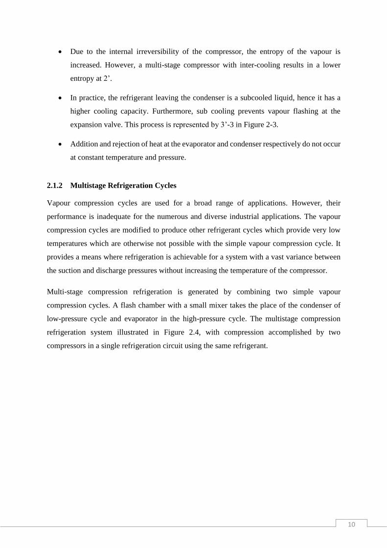
Figure 2-6 : Two-Stage Cascade Refrigeration Cycle. ........................................................... 13
Figure 2-7 : Temperature-entropy diagram for Cascade Refrigeration system (Extracted from
Çengel and Boles, 2006). ......................................................................................................... 14
Figure 2-8 : Flowchart for the Exergy Analysis for a VCRS with two-Evaporators (Extracted
from Yataganbaba et al., 2015). ............................................................................................... 22
Figure 3-1 : Comparison of Pressures of Lower Boiling and Higher Boiling Refrigerants at
given Evaporator and Condenser Temperature. (Extracted from Arora, 2009). ..................... 25
Figure 3-2 : An (a) azeotropic refrigerant and (b) near-azeotropic refrigerant blend at a given
pressure as they boil (Extracted from Whitman et al., 2013). ................................................. 28
Figure 4-1 : Experimental set-up for R12, R134a, and R290/600a investigation (Extracted
from Mani and Selladurai, 2008). ............................................................................................ 36
Figure 4-2 : The breadboard heat pump (Extracted from Jung et al., 2000). .......................... 38
Figure 4-3 : Schematic of the refrigeration unit (Extracted from Halimic et al., 2003). ........ 39
Figure 4-4 : Schematic representation of the air/air heat pump test unit (Extracted from Sami
and Desjardins, 2000). ............................................................................................................. 40
Figure 4-5 : Schematic of the experimental setup for the performance test of CO2/propane
mixture (Extracted from Kim et al., 2007). ............................................................................. 41
Figure 4-6 : Schematic of the multi-cycle R744 test rig (Extracted from Chesi et al., 2012). 42
Figure 4-7 : Layout of the thermal load management system (Extracted from Chesi et al.,
2012). ....................................................................................................................................... 43
Figure 5-1 : Original schematic of the test unit (Produced by Shadrach, 2014). .................... 47
Figure 5-2 : Stainless Steel vibration eliminator (Extracted from Heldon, 2009b). ............... 49
Figure 5-3: Flow diagram of a single-pass counter flow arrangement (Extracted from Kakac
et al., 2012). ............................................................................................................................. 51
Figure 5-4 : A Cross-sectional view of a Suction Accumulator (Extracted from Heldon,
2009a). ..................................................................................................................................... 53
Figure 5-5 : Schematic Design of Modified test unit .............................................................. 64
Figure 6-1 : Recovery Unit and the refrigeration system (Extracted from Dennis et al., 2010).
.................................................................................................................................................. 69
Figure 7-1 : Compressor Work vs. Coefficient of performance (COP). (*) R507, (▲) R413a,
(●) R134a. ................................................................................................................................ 87

xiii
Figure 7-2 : Evaporating Temperature vs. Coefficient of performance (COP), (*) R507, (▲)
R413a, (●) R134a ..................................................................................................................... 88
Figure 7-3 : Condensing Temperature vs. Compressor Work, (▲) R413a, (●) R134a .......... 89
Figure 7-4 : Condensing Temperature vs. Coefficient of performance (COP), (▲) R413a, (●)
R134a. ...................................................................................................................................... 90
Figure 7-5 : Cooling effect vs. Coefficient of performance (COP), (*) R507, (▲) R413a, (●)
R134a ....................................................................................................................................... 91
Figure 7-6 : Condenser Water flowrate vs. Coefficient of performance (COP), (▲) R507, (●)
R134a ....................................................................................................................................... 92
Figure 7-7 : Condenser water flowrate vs. Compressor discharge temperature, (▲) R507, (●)
R134a. ...................................................................................................................................... 93
Figure 7-8 : Refrigerant charge vs. compressor discharge temperature, (▲) R413a, (●)
R134a ....................................................................................................................................... 94
Figure 7-9 : Refrigerant charge vs Compressor Efficiency, (▲) R413a, (●) R134a. ............. 94
Figure 7-10 : Condenser and Evaporator water flowrate vs Evaporator Refrigerant
Temperature. (right (●) R134a), left (▲) R507) ..................................................................... 95
Figure 7-11 : Flowsheet of a single vapour compression cycle with Hot and Cold fluid
cycles........................................................................................................................................ 96
Figure A.1 : Temperature profiles of heat exchanger during the phase change of (a) pure
refrigerant, (b) zeotropic refrigerant mixture with glide matching. (Rajapaksha, 2007). ...... 119
Figure A.2 : Pressure and temperature profile for condensation of a non-azeotropic mixture.
(Jung et al., 2003)................................................................................................................... 121
Figure C.1 : Simple VC configuration. ................................................................................. 125
Figure C.2 : VC configuration using two compressors. ....................................................... 126
Figure C.3 : Configuration for VC with suction line heat exchanger. .................................. 127
Figure C.4 : Cascade VC cycle configuration ...................................................................... 128
Figure C.5 : Two-stage VC cycle configuration. .................................................................. 129

xiv
List of Tables
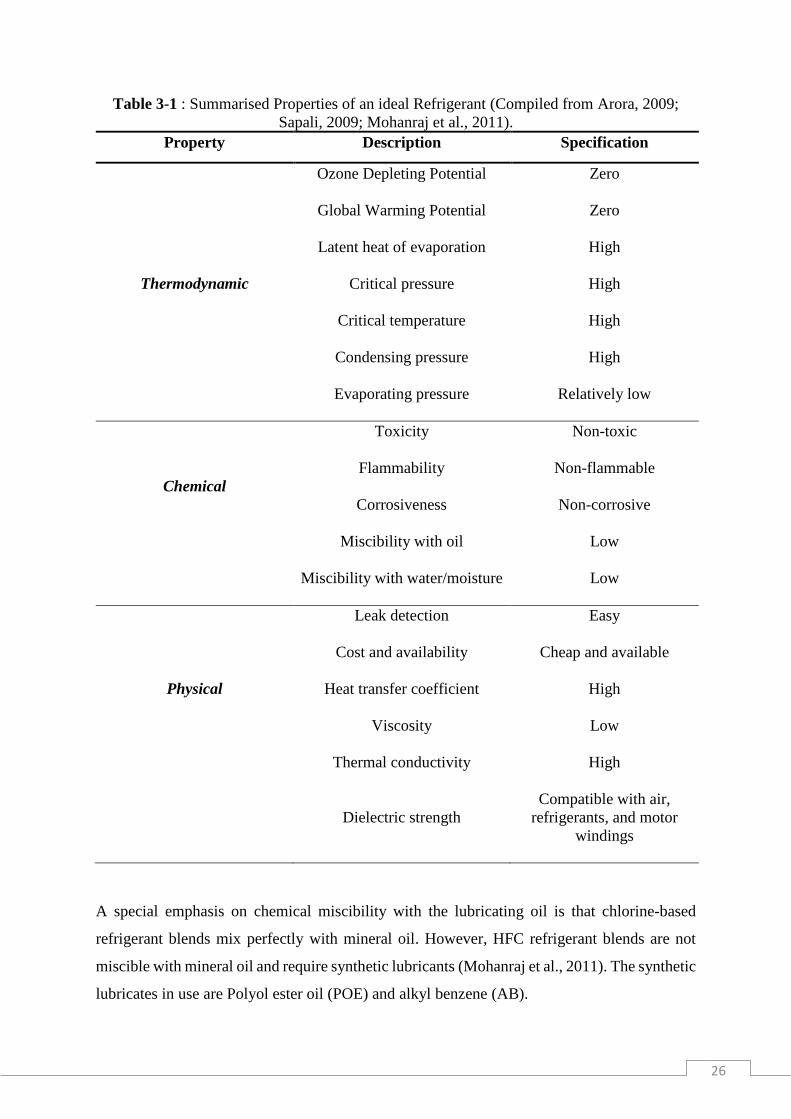
Table 3-1 : Summarised Properties of an ideal Refrigerant (Compiled from Arora, 2009;
Sapali, 2009; Mohanraj et al., 2011). ....................................................................................... 26
Table 3-2: A Review of Studies published on Refrigerants and Refrigerant Blends. ............. 30
Table 5-1 : Geometric Specifications of the Heat Exchangers. .............................................. 52
Table 5-2 : Specifications of Instruments ............................................................................... 57
Table 7-1 : Details of the chemicals used in this study. .......................................................... 73
Table 7-2 : Thermodynamic Properties of Refrigerants.......................................................... 74
Table 7-3 : Temperature Sensors Calibration Details. ............................................................ 75
Table 7-4 : Pressure Transducers Calibration Details. ............................................................ 75
Table 7-5 : Uncertainties in measurements related to this study............................................. 76
Table 7-6 : Results during commissioning of unit using R134a. ............................................ 78
Table 7-7 : Effects of the Condenser Flowrate on system. ..................................................... 80
Table 7-8 : Effects of Refrigerant Mass on the system. .......................................................... 81
Table 7-9 : Comparison of Effects of Power Settings on the system. ..................................... 82
Table 7-10 : Comparison of Refrigerant Properties at different degrees of throttling. ........... 83
Table 7-11 : Comparison of Experimental results to literature for R134a with Evaporator (4-5 oC) and Condenser (40 oC). ...................................................................................................... 85
Table 7-12 : Specification of Simulation Variables. ............................................................. 101
Table 7-13 : Comparison of Simulated COP results for refrigerants and refrigerant blends.
................................................................................................................................................ 102
Table 7-14 : Comparison of the experimental and simulated results for R134a. .................. 103
Table 7-15 : Comparison of the Experimental and simulated results for R507. ................... 104
Table 7-16 : Comparison of the experimental and simulated results for R413a. .................. 105
Table 7-17 : Comparison of simulated results for R134a, R125, and R134a/R125 blends. . 107
Table A.1: Azeotropic Refrigerant blends temperature glide for selected CFCs/HCFCs
replacements determined at 100kPa. (Rajapaksha, 2007). .................................................... 119
Table B.1 : Compressor Specifications ................................................................................. 122
Table B.2 : Valves Specifications (Swagelok Company, 2013). .......................................... 122
Table E.1 : Simulation Results for R413a ............................................................................ 133
Table E.2 : Simulation Results for R134a ............................................................................ 134
Table E.3 : Simulation Results for R134a/R125 (50/50 wt %) ............................................. 135
Table E.4 : Simulation Results for R134a/R125 (66/34 wt %) ............................................. 136
Table E.5 : Simulation Results for R507 .............................................................................. 137
Table E.6 : Simulation Results for R125 .............................................................................. 138
Table G.1 : List of Refrigerants used in this study ............................................................... 141

1
Chapter 1
1 Introduction
Until recently, contemporary refrigeration technology used for temperature regulation within
built structures and the preservation of perishables, was dependent largely on
chlorofluorocarbons and hydrochlorofluorocarbons as refrigerants. This dependence was due
to their excellent physical and thermodynamic properties. However, these refrigerants are being
phased out from the market due to their adverse environmental impact.
This project is in line with the ongoing global research on refrigerants and refrigerant blends.
It seeks to come up with the most fitting substances to replace chlorofluorocarbons (CFCs) and
hydrochlorofluorocarbons (HCFCs). The application of CFC-free refrigerant blends also
provides a means of assisting air-conditioning and refrigeration industries in complying with
the CFC phase-out provision, (Szymurski (2005) and Goetzler et al. (2014)), under the
Montreal Protocol, without harming the interests of end users.
This study which investigates new refrigerant blends and use of fluorochemicals, also concurs
with the South African Fluorochemicals Expansion Initiative (FEI) research which seeks to
explore the use of fluorochemicals and fluorine products in various areas across multiple
market sectors (Pelchem, 2014). The program was launched by the Government in 2008 (South
African Government Press Release, 2009), through Pelchem, a chemical division of the
Nuclear Energy Corporation of South Africa. These include fluorocarbons which can be
converted to refrigerants and refrigerant blends, consequently tapping into the fluorspar
reserves which are abundant in the country. Utilisation and beneficiation of the fluorspar
reserves will promote the economic development of the nation.
1.1 Environmental Impact of Refrigerants
Molina and Rowland (1974), stated that the chlorine ion in chlorofluorocarbons (CFCs) was
responsible for the destruction of the stratosphere’s ozone layer. The ozone layer protects the
earth surface by absorbing the sun’s UV rays. CFCs have a long lifespan (Satyanarayana and
Kotaiah, 2012). Therefore, a single chlorine molecule in the stratosphere repeatedly reacts with,
and causes deterioration of ozone molecules, leading to a “hole” in the ozone layer (Angell,
1988; Sivasakthivel and Reddy, 2011). The discovery of the hole in the ozone layer marked

2
the beginning of the decline in the widespread use of CFCs and HCFCs, which in turn, provides
the motivating factor for research into alternative refrigerants.
By the 1980s, the destruction of ozone by refrigerants caught the attention of the international
community leading to a number of international agreements which affected the refrigeration
industry. In the year 1987, 27 nations convened in Montreal Canada, and signed a global
environment treaty. Under this agreement, industrialised countries were obliged to begin
phasing out CFCs by 1993, and to achieve a 50% reduction relative to 1986 consumption levels,
by 1998 (United Nations Montreal Protocol, 1987). At meetings in London (1990) Copenhagen
(1992), Vienna (1995), Montreal (1997) and Beijing (1999) amendments were adopted with
the intention of speeding up the phasing out of ozone-depleting substances (United States EPA,
2007). In the year 2014, a proposal, by Mexico, Canada, and the United States, was made to
amend the Montreal Protocol to cut the production and use of hydrofluorocarbons (HFCs) by
85% in the period 2016-2035 for industrialised countries (United Nations EPA, 2014).
Due to the adverse effects of climate changes, and the escalation of greenhouse gases in the
atmosphere from uncontrolled emissions, 192 nations convened in Kyoto Japan in 1997 and
penned a concord, which became known as the Kyoto Protocol (Baxter et al., 1998). Under this
agreement, countries were to reduce the discharge of greenhouse gases (by 5% by the year
2012 relative to the 1990 emission levels) and lessen the use of global warming potential
(GWP) substances (Breidenich et al., 1998). All halocarbon refrigerants are categorised as
GWP substances, and their presence in the atmosphere contributes to global warming. A total
equivalent warming index (TEWI) method was developed to quantify and analyse the
greenhouse effect caused by the emission of refrigerants’ from a refrigeration system (Bitzter,
2014). Also, the environmental impact of the refrigerant over the entire life cycle of the fluid
and the equipment was evaluated with the life cycle climate performance (LCCP) formula. The
lower the LCCP for a refrigerant the lesser is its environmental impact, hence, the more
desirable it will be for refrigeration applications (Abdelaziz et al., 2012).
As a result of the current environmental regulations, based upon scientific findings, stipulations
have been made that refrigerants must be; substances with lower global warming potential,
zero ozone depletion potential (ODP), and comply with requirements for safety, material
compatibility, and suitability (Calm, 2008). Hydrochlorofluorocarbon (HCFC) refrigerant
mixtures and hydrofluorocarbons (HFCs) have proven to be suitable replacements possessing
most of the required properties (Akintunde, 2013). Hydrofluorocarbon mixtures and

3
hydrocarbons have a short atmospheric lifetime making them attractive for use in air
conditioning and refrigeration systems (Sekiya and Misaki, 2000). Hydrocarbon refrigerants
such as isobutene, propane and n-butane are considered for refrigeration due to the ODP and
GWP effects of the current refrigerants. However, the main shortcoming of hydrocarbons in
refrigeration is their high flammability (Mani et al., 2013).
1.2 Background to the Study
The motivation to design the refrigerant unit in this study was driven by the need to be able to
test different refrigerants and refrigerant blends over a wide range of operating conditions using
different refrigeration cycle configurations. Furthermore, it seeks to address the practical aspect
of the theoretical study carried out by Satola (2014) within the Thermodynamics Research Unit.
Satola worked on a predictive tool to enable development of suitable refrigerant combinations
which are environmental friendly for use in refrigeration applications. This was performed
using computational software ASPEN Plus ® along with Dortmund Data Bank (DDB)
imported into Visual Basic for Applications (VBA) project. In his work, he proposed many
refrigerant blends which can be utilised as replacements for R22 refrigerant.
The refrigeration test rig utilised in this study was designed and built in the Thermodynamics
Research Unit in 2012 by Ms Alisha Kate Shadrach a MSc. Eng. Student under the supervision
of Professors J.D Raal, P Naidoo, and D Ramjugernath. While the unit was assembled in 2014,
it was not commissioned. Shadrach did not overcome the issues of sealing in achieving very
low pressures/vacuum in the refrigeration system. Hence further test measurements could not
be performed. There were also various problems encountered in the piping and location and/or
installation of key units.
In this study, major modifications were performed to deem the unit suitable for experimental
measurements. These included overcoming the challenge of pressure loss in the experimental
unit. This pressure loss was mainly due to leaks in the condenser seals, vibration eliminators
and in many loose joints in the unit. To achieve the throttling effect there was also a need to
remove the metering valve due to its small orifice which was a hindrance to the passage of the
liquid refrigerant to the expansion valve. Furthermore, there was a need to replace the water
baths at the condenser and evaporator with larger ones to meet the duties of these two heat
exchangers.

4
The unit was designed to operate in several thermodynamic (refrigeration) cycles namely: the
simple vapour compression cycle, two-stage vapour compression cycle, cascade system and
vapour compression cycle with a suction-line heat exchanger. The novelty of the design is the
selection of compressors with variable drive motors used to vary the operating conditions over
a wide range and thus enabling the operator to adjust compressor speed to suit the type of
refrigerant under investigation. The refrigeration unit will allow for a preliminary evaluation
of the performance (and hence suitability), of the proposed new refrigerant blends in
refrigeration applications; and the identification of optimum operating ranges in different
cycles.
In this study, it was necessary to first commission the test unit. This was achieved by ensuring
that the unit was sealed and could maintain a vacuum level of 26.6 kPa abs. Refrigerant R134a
was used to test the unit to deem it functional and suitable for refrigeration experimental work
by obtaining repeatable and reproducible experimental results which were comparable to
published data. Two commercial blends, R413a and R507a, were proposed for investigations
so that their performance could be compared with that of R134a, and their suitability for
replacing R134a in its refrigeration cycles. Laboratory synthesised mixtures of R134a/R125 in
different weightings were then studied and their performance was compared to that of R134a,
R507a, and R413a.
Vapour compression refrigeration cycle simulations were performed using the REFPROP
program in Aspen Plus V8.6, an engineering software package, to compare the performance of
the simulations (ideal) with experimental results.
1.3 Thesis Overview
In this study, the performance of two commercial refrigerant blends, R413a and R507 as well
as a laboratory synthesised blend composed of R134a/R125 in the ratios 50/50 and 66/34 by
wt.% were analysed in a vapour compression refrigeration cycle (VCRS). Refrigerant R134a
was used as the benchmark in the study.
Chapter two briefly explains the principles of refrigeration. It describes the purpose of each
component in the refrigeration cycle, different refrigeration cycles, and the energy as well
exergy analysis of the vapour compression refrigeration cycles.

5
Chapter three presents a literature review on refrigerant blends and their environmental effects.
It also describes the nature of different refrigerants and its properties. Literature data is
presented from studies performed on R134a, R413a, R507 and various refrigerant blends. In
the fourth Chapter, equipment reviews of the refrigerant test units previously employed for
refrigeration studies is presented.
The description of the refrigeration unit used in this study is presented in Chapter five. Chapter
six outlines the experimental procedure followed in operating the unit. The results obtained in
this study are presented and discussed in Chapter seven. These include the chemical purity and
physical properties of the refrigerants, uncertainty in measurements, commissioning results
obtained, compatible analysis of the performance of the refrigerant blends in the test rig and
the simulation results. Lastly, the conclusions and recommendations are provided in Chapter
eight and nine respectively.
6
Chapter 2
2 Principles of Refrigeration
Refrigeration utilises a chemical substance to maintain a low-temperature environment by
continuously rejecting heat to a higher temperature environment when the vapour produced is
condensed for reuse. The absorption of heat is traditionally achieved by the evaporation of a
liquid in a continuous flow process. In the refrigeration cycle, the direction of heat transfer is
from a lower temperature point to an elevated temperature point. However, according to the
second law of thermodynamics, this is not possible without an external supply of energy (Smith
et al., 2005).
Vapour compression systems are widespread in refrigeration. In these systems, a vapour
cycling process causes the working fluid, also known as the refrigerant to undergo phase
changes. For the refrigeration process to occur a continuous removal of heat from the low-
temperature point must occur. This cooling can be achieved by evaporating the liquid
refrigerant in a steady-state flow process. The vapour can be returned to its original liquid state
to be re-evaporated either one of two ways:
• it can simply be compressed and then condensed;
• it can be absorbed by a less volatile liquid, whence it can be evaporated at an elevated
pressure (Smith et al., 2005).
To fully comprehend the refrigeration cycle, the Carnot vapour refrigeration cycle must be
understood, as the operation of the refrigeration cycle is derived from that of the Carnot cycle
(the most efficient cycle with the highest coefficient of performance (COP).
2.1 Refrigeration Cycles
2.1.1 Vapour Compression Refrigeration Cycle
The principle of operation of vapour refrigeration originated from a reversed Carnot power
cycle. In the vapour compression cycle, the turbine in the Carnot cycle is replaced with a
throttling device which can be an expansion valve, an expansion engine or capillary tube. It is
cheaper to use an expansion valve or capillary tube than an expansion engine due to the high
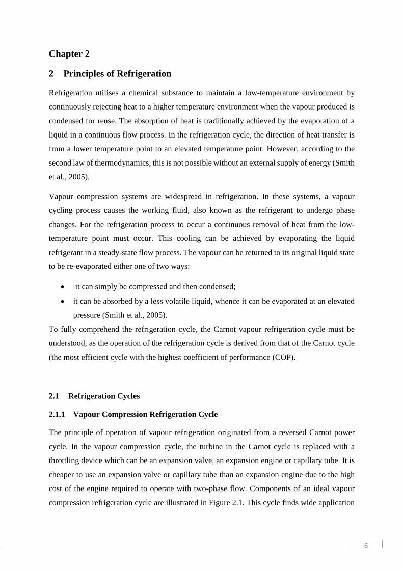
cost of the engine required to operate with two-phase flow. Components of an ideal vapour
compression refrigeration cycle are illustrated in Figure 2.1. This cycle finds wide application
7
in refrigerators, heat pumps and air conditioning systems. Figure 2.1 shows work and energy
transfer when the system is operating in a steady state. A brief description of the units in the
cycle is given below.
Expansion valve Compressor
Condenser
Evaporator
3
4 1
2
Figure 2-1: Components of Vapour-Compression Refrigeration Cycle.
Evaporator
The low pressure, cool liquid-vapour refrigerant passes through the evaporator where it
interacts with the heat load or the medium to be maintained at a low temperature. The low-
pressure refrigerant in the evaporator absorbs heat from the medium to be cooled and boils,
producing low-pressure vapour at saturation conditions.
Compressor
The saturated vapour exits the evaporator and then passes into the compressor. The addition of
shaft work to the saturated vapour raises its pressure. When the pressure of the refrigerant
increases, the boiling and condensing temperatures of the refrigerant are elevated as well.
Sufficiently compressing the gas raises its boiling point higher than the temperature of the heat
sink (cooling medium), which is the higher temperature medium of the system.
Condenser
The compressed high-pressure gas carrying heat energy acquired at the evaporator as well as
from the work done by the compressor (in gas-compression and due to friction) enters the
condenser. The high-pressure refrigerant changes phase at constant temperature and pressure

8
to a saturated liquid as it rejects heat to the system’s heat sink. The heat source (high-pressure
vapour) is condensed as it transfers heat energy to the heat sink.
Expansion Valve
The pressurized saturated liquid refrigerant expands at the throttling valve to the evaporator
pressure. An irreversible adiabatic expansion resulting in the decrease in refrigerant pressure,
as well as an increase in entropy occurs. At the valve’s outlet, a liquid-vapour mixture of the
refrigerant is obtained.
The performance of the ideal vapour –compression cycle can be evaluated if the irreversibilities
within the compressor, condenser and evaporator are neglected. Therefore, no pressure drops
due to friction are experienced. This also means there are no pressure losses due to refrigerant’s
flows through the heat exchangers. If the compression of the refrigerant occurs without
irreversibility and heat losses from the system, then the compression process is isentropic.
Considering the above assumptions, the temperature-entropy diagram for a vapour-
compression refrigeration cycle is shown in Figure 2.2.
Figure 2-2 : T-S diagram of an ideal vapour- compression cycle.(Extracted from Moran and
Shapiro, 2006).
The ideal cycle is made up of the following sequence of processes:
Process 1-2s: The refrigerant vapour is compressed isentropically from the evaporator pressure
at state 1 to the condenser pressure at state 2s.
9
Process 2s-3: Isobaric cooling occurs from point 2s to the vapour saturation curve.
Subsequently, the gaseous refrigerant loses heat as it transverses through the condenser at
constant pressure. The refrigerant leaves the condenser as saturated liquid at state 3.
Process 3 -4: Isenthalpic expansion of the saturated liquid refrigerant from state 3 to a liquid –
vapour mixture (two-phase mixture) at stage 4.
Process 4- 1: Evaporation of liquid refrigerant at a constant (low) pressure and temperature, as
heat is absorbed from the surroundings/ heat transfer fluid.
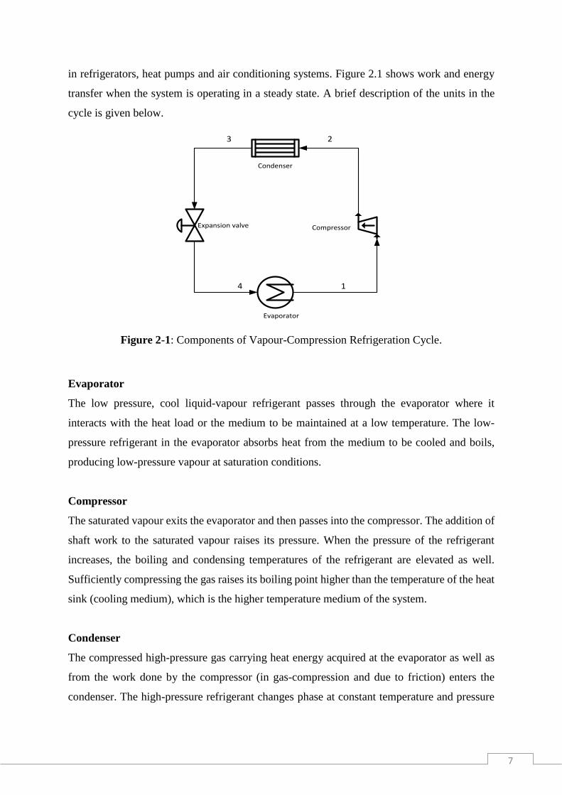
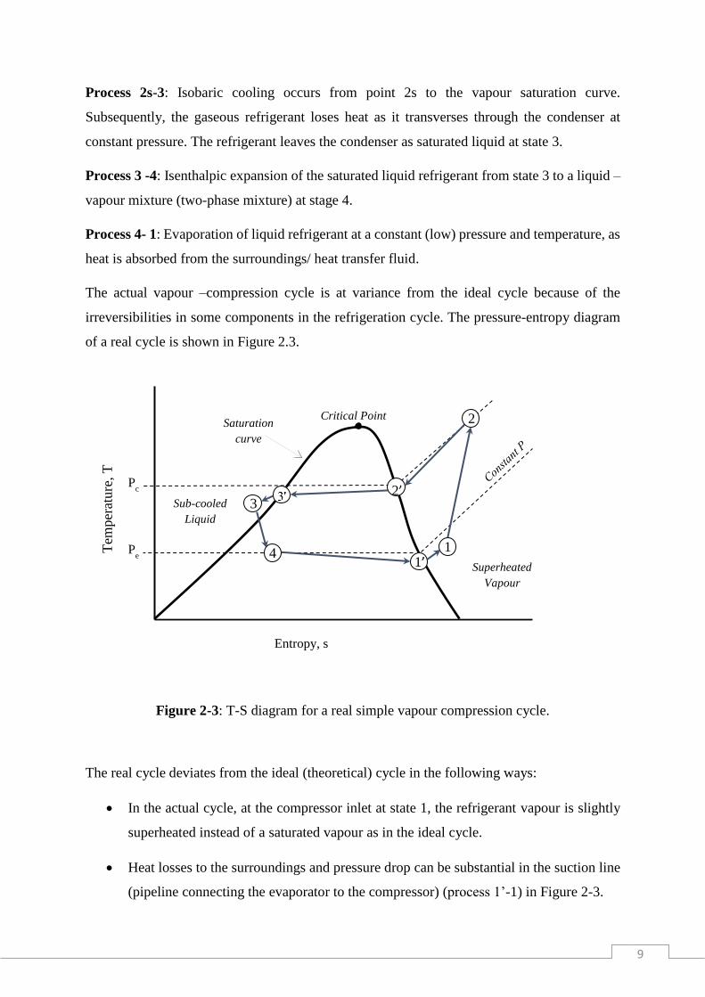
The actual vapour –compression cycle is at variance from the ideal cycle because of the
irreversibilities in some components in the refrigeration cycle. The pressure-entropy diagram
of a real cycle is shown in Figure 2.3.
Figure 2-3: T-S diagram for a real simple vapour compression cycle.
The real cycle deviates from the ideal (theoretical) cycle in the following ways:
• In the actual cycle, at the compressor inlet at state 1, the refrigerant vapour is slightly
superheated instead of a saturated vapour as in the ideal cycle.
• Heat losses to the surroundings and pressure drop can be substantial in the suction line
(pipeline connecting the evaporator to the compressor) (process 1’-1) in Figure 2-3.
Sub-cooled
Liquid
Saturation
curve
Superheated
Vapour
Entropy, s
Tem
per
ature
, T
Critical Point
Pc
Pe
4 1
1’
2
3
2’
10
• Due to the internal irreversibility of the compressor, the entropy of the vapour is
increased. However, a multi-stage compressor with inter-cooling results in a lower
entropy at 2’.
• In practice, the refrigerant leaving the condenser is a subcooled liquid, hence it has a
higher cooling capacity. Furthermore, sub cooling prevents vapour flashing at the
expansion valve. This process is represented by 3’-3 in Figure 2-3.
• Addition and rejection of heat at the evaporator and condenser respectively do not occur
at constant temperature and pressure.
2.1.2 Multistage Refrigeration Cycles
Vapour compression cycles are used for a broad range of applications. However, their
performance is inadequate for the numerous and diverse industrial applications. The vapour
compression cycles are modified to produce other refrigerant cycles which provide very low
temperatures which are otherwise not possible with the simple vapour compression cycle. It
provides a means where refrigeration is achievable for a system with a vast variance between
the suction and discharge pressures without increasing the temperature of the compressor.
Multi-stage compression refrigeration is generated by combining two simple vapour
compression cycles. A flash chamber with a small mixer takes the place of the condenser of
low-pressure cycle and evaporator in the high-pressure cycle. The multistage compression
refrigeration system illustrated in Figure 2.4, with compression accomplished by two
compressors in a single refrigeration circuit using the same refrigerant.

11
Expansion Valve
High PressureCompressor
Condenser
Evaporator
5 4
ExpansionValve
Low PressureCompressor
8
WHP
WLP
QLP
QHP
FlashingChamber
6
72
3
9
1
Figure 2-4 : Multistage Compression Refrigeration System with a Flashing Chamber.
Liquid refrigerant leaving the condenser expands as it passes through the throttling valve in the
line 5-6 to the flash chamber. Partial vaporization of the liquid occurs, the saturated vapour
then passes via line 3 then mixes with the superheated vapour from the low-pressure
compressor coming via line 2. The mixture passes into the high-pressure compressor via line 9
for further compression, This is a regeneration process. The liquid coming from the flash
chamber in state 7 is saturated, it is throttled at the second expansion valve then enters the
evaporator where it draws heat from the environment to be cooled.

12
Figure 2-5 : Temperature-entropy diagram of a Multi-stage Compression System.(Extracted
from Çengel and Boles, 2006).
The condenser and evaporator can have significantly large pressure and temperature
differences in this system. The compression process in this cycle arrangement is executed in a
two-stage compression process with intercooler, hence the compressor work decreases.
2.1.3 Cascade Refrigeration Systems
A cascade refrigeration system utilises two different refrigerants having different physical
properties which run through two independent refrigeration cycles. These cycles are linked by
a heat exchanger which operates as a condenser in the low-temperature cycle at the same time
being an evaporator in the high-temperature cycle. This system is ideal for conditions where
there is a substantial pressure difference between the evaporator and the condenser. A large
temperature difference means a large pressure difference as well. To overcome this situation,
the refrigerant systems are arrayed in a parallel connection resulting in a cascade system of
vapour compression cycles.
A two-stage cascade refrigeration system, in Figure 2.6 shows the heat exchanger connecting
the two cycles, it serves as an evaporator for cycle A (High-temperature circuit) and the
condenser for cycle B (Low-temperature circuit).
13
Expansion Valve Compressor
Condenser, Tc
Evaporator, TE
76
Heat Exchanger
Expansion Valve Compressor
8
3
4 1
5
2
High Temperature
circuit
Low Temperature
circuit
THEE
THEC
WHT
WLT
QLT
QHT
Figure 2-6 : Two-Stage Cascade Refrigeration Cycle.
The temperature-entropy diagram for a cascade system is shown in Figure 2.7. It can be noted
that the cascade system increases the refrigeration effect and decreases the compressor power
when compared to a simple VCC. These effects result in an overall increase of the refrigeration
system’s COP.

14
Figure 2-7 : Temperature-entropy diagram for Cascade Refrigeration system (Extracted from
Çengel and Boles, 2006).
There are two thermodynamic methods used to gauge the performance of energy conversion
systems, namely energy analysis and exergy analysis. Although energy analysis finds wide use
and application, exergy analysis is more valuable as it not only measures the proximity of the
system to the ideal operation but also identifies the system components subject to
thermodynamic losses and irreversibilities. The results of exergy and energy analysis are
expressed in the forms of energy and exergy efficiency indicators. These two are the key
performance indicators in refrigeration.
2.2 Energy Analysis
All the major components in the vapour compression cycle shown in Figure 2.1 are internally
reversible except for the throttling process. Since all the four components in the vapour-
compression refrigeration cycle are steady-flow units, therefore, it is referred to as an ideal
cycle. For this reason, the analyses of all the cycle components processes can be done under
steady-flow conditions (Moran and Shapiro, 2006):

15
��𝐶𝑉 = ∑ (ℎ +𝑢2
2+ 𝑔𝑧)
0 𝑜
𝑚𝑜 − ∑ (ℎ +𝑢2
2+ 𝑔𝑧)
𝑖 𝑖
𝑚𝑖 + ��𝐶𝑉 2.1a
Where ��𝐶𝑉 is the rate of heat transfer between the control volume and its surroundings [J/s] ,
h is the specific enthalpy [J/kg] , ��𝐶𝑉 is the energy crossing the boundary of a closed system
[J/s], 𝑚𝑜 and 𝑚𝑖 are inlet and outlet mass flow rates, 𝑢2
2 is the kinetic energy term, and 𝑔𝑧 the
potential energy term.
The potential and kinetic energy changes of the refrigerant across the cycle’s components are
small and thus can be neglected. Considering only work and heat transfer terms;
��𝐶𝑉 = ℎ𝑜��𝑜 − ℎ𝑖��𝑖 + ��𝐶𝑉 2.1b
Then the steady-state equation on a unit mass basis assuming constant mass flow rate in the
system reduces to:
𝑞 − 𝑤 = ℎ𝑜 − ℎ𝑖 2.1c
where q is the heat transfer per unit mass [J/kg], Q is the rate of heat transfer between the
control volume and its surroundings [J/s], m is the mass flow rate of the refrigerant [kg/s] and
w is the work done per unit mass of the system.
Evaporator
Considering the refrigerant side of the evaporator as the control volume, denoted by 4-1 in
Figures 2.1 and 2.7 the energy and mass rate balances (Equation 2.1b) gives the rate of heat
transfer per unit mass of the refrigerant flowing as:
��𝑖𝑛
�� = ℎ1 - ℎ4 2.2
Compressor
16
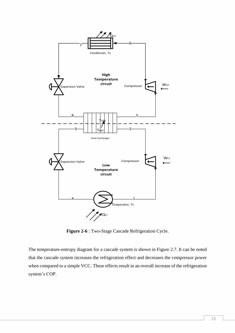
Supposing no heat exchange occurs between the compressor and its surroundings, the energy
and mass rate balances for a control volume encircling the compressor gives:
��𝑐
�� = ℎ2 - ℎ1 2.3
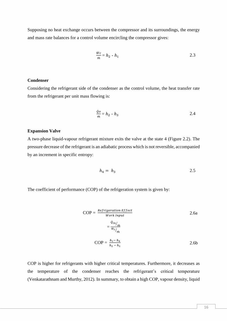
Condenser
Considering the refrigerant side of the condenser as the control volume, the heat transfer rate
from the refrigerant per unit mass flowing is:
��𝑜
�� = ℎ2 - ℎ3 2.4
Expansion Valve
A two-phase liquid-vapour refrigerant mixture exits the valve at the state 4 (Figure 2.2). The
pressure decrease of the refrigerant is an adiabatic process which is not reversible, accompanied
by an increment in specific entropy:
ℎ4 = ℎ3 2.5
The coefficient of performance (COP) of the refrigeration system is given by:
COP = 𝑅𝑒𝑓𝑟𝑖𝑔𝑒𝑟𝑎𝑡𝑖𝑜𝑛 𝐸𝑓𝑓𝑒𝑐𝑡
𝑊𝑜𝑟𝑘 𝐼𝑛𝑝𝑢𝑡2.6a
= ��𝑖𝑛
��⁄
��𝑐��
⁄
COP = ℎ1− ℎ4
ℎ2 − ℎ12.6b
COP is higher for refrigerants with higher critical temperatures. Furthermore, it decreases as
the temperature of the condenser reaches the refrigerant’s critical temperature
(Venkatarathnam and Murthy, 2012). In summary, to obtain a high COP, vapour density, liquid
17
thermal conductivity, and latent heat should have high values. Whereas molecular weight and
liquid viscosity values should be low (Prapainop and Suen, 2012).
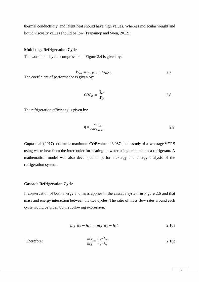
Multistage Refrigeration Cycle
The work done by the compressors in Figure 2.4 is given by:
𝑊𝑖𝑛 = 𝑤𝐿𝑃,𝑖𝑛 + 𝑤𝐻𝑃,𝑖𝑛 2.7
The coefficient of performance is given by:
𝐶𝑂𝑃𝑅 =𝑄𝐿𝑃
𝑊𝑖𝑛 2.8
The refrigeration efficiency is given by:
𝜂 = 𝐶𝑂𝑃𝑅
𝐶𝑂𝑃𝐶𝑎𝑟𝑛𝑜𝑡 2.9
Gupta et al. (2017) obtained a maximum COP value of 3.087, in the study of a two stage VCRS
using waste heat from the intercooler for heating up water using ammonia as a refrigerant. A
mathematical model was also developed to perform exergy and energy analysis of the
refrigeration system.
Cascade Refrigeration Cycle
If conservation of both energy and mass applies in the cascade system in Figure 2.6 and that
mass and energy interaction between the two cycles. The ratio of mass flow rates around each
cycle would be given by the following expression:
��𝐴(ℎ5 − ℎ8) = ��𝐵(ℎ2 − ℎ3) 2.10a
Therefore: ��𝐴
��𝐵 =
ℎ2−ℎ3
ℎ5−ℎ8 2.10b

18
Also, the coefficient of performance is given by:
𝐶𝑂𝑃𝑅,𝑐𝑎𝑠𝑐𝑎𝑑𝑒 = ��𝐿𝑇
��𝑛𝑒𝑡,𝑖𝑛
=��𝐵(ℎ1 − ℎ4)
��𝐴(ℎ6 − ℎ5) + ��𝐵(ℎ2 − ℎ1)
2.11
Hoşöz (2005), in the analysis of a single stage and cascade system noted that the overall COP
value for the cascade system was lower than the one for a single stage system. This scenario
was caused by high power requirement of the higher unit compressor in the cascade system. In
deriving the above expressions, the assumption made was that the refrigerants are the same in
both cycles which would not necessarily be the case.
2.3 Exergy Analysis
Exergy is the highest possible work which a system can produce as it undertakes a reversible
process from a defined original state to that of its environment, which is termed a dead state
(Çengel and Boles, 2006). Practically it may be defined as a measure of the system’s ability to
bring about change because of not being in equilibrium with a reference (dead) state. A system
is said to be in dead state when in thermodynamic equilibrium with its surroundings, i.e., it is
the same temperature, pressure and is chemically unreactive with its environment. The exergy
of a system at dead state is zero.
A flowing stream has exergy associated with it in addition to flow energy which is needed to
sustain the flow. The stream specific exergy is denoted by the symbol, e (Yataganbaba et al.,
2015):
𝑒 = (ℎ − ℎ𝑜 ) – 𝑇𝑜 (𝑠 − 𝑠𝑜) +𝑉2
2+ 𝑔𝑧 2.12
Where 𝑠𝑜 and ℎ𝑜 are the entropy and enthalpy values of the dead state at temperature 𝑇𝑜, 𝑉2
2
and 𝑔𝑧 are the kinetic and potential exergy terms, respectively.
Exergy transfer by heat:
19
𝑋ℎ𝑒𝑎𝑡 = (1 −𝑇𝑜
𝑇) 𝑄 2.13
Exergy transfer by mass:
𝑋𝑚𝑎𝑠𝑠 = 𝑚 𝑒 2.14
Exergy transfer by work:
𝑋𝑤𝑜𝑟𝑘 = {𝑊 − 𝑊𝑠𝑢𝑟𝑟 (𝑓𝑜𝑟 𝑏𝑜𝑢𝑛𝑑𝑎𝑟𝑦 𝑤𝑜𝑟𝑘)
𝑊 (𝑓𝑜𝑟 𝑜𝑡ℎ𝑒𝑟 𝑓𝑜𝑟𝑚𝑠 𝑜𝑓 𝑤𝑜𝑟𝑘) 2.15
All the equipment in the refrigeration unit operate under steady state condition; they do not
undergo any changes in their energy, mass, entropy, and energy. Therefore, the rate of the
generated exergy for steady flow is:
∑ (1 −𝑇𝑜
𝑇𝑘) ��𝑘 − �� + ∑ ��
𝑖𝑛
𝑒 − ∑ ��
𝑜𝑢𝑡
𝑒 − ��𝑑𝑒𝑠𝑡𝑟𝑜𝑦𝑒𝑑 − 0 2.16
In the four main components of the refrigerant system exergy is destroyed or consumed due to
entropy generated depending on the related processes. In the exergy analysis for components
in the VCRS, the following assumptions were made:
i. All components remain in steady state conditions.
ii. Neglecting pressure losses in the pipelines.
iii. Heat exchange between the system and its surroundings are considered negligible.
iv. Potential and kinetic energy, as well as exergy losses, are ignored (Ahamed et al.,
2011).
The mathematical formula for exergy destroyed in each unit in the cycle is given below for
component (Stanciu et al., 2011; Yataganbaba et al., 2015):
• For the evaporator (ev):

20
𝐼𝑒𝑣 = ��4 − ��1 + 𝑄𝑣(1 −𝑇𝑜
𝑇𝑣) 2.17a
where I is the exergy destruction rate computed in watts and �� is exergy
Replacing equation (2.12) into the above equation:
𝐼𝑒𝑣 = ��[(ℎ4 − 𝑇𝑜𝑠4) − (ℎ1 − 𝑇𝑜𝑠1)] + 𝑄𝑣(1 −𝑇0
𝑇𝑣) 2.17b
Substituting equation (2.16) in the other components:
• For the condenser (c):
𝐼𝐶 = ��2−��3 2.18a
𝐼𝑐 = ��[(ℎ2 − 𝑇𝑜𝑠2) − (ℎ3 − 𝑇𝑜𝑠3)] 2.18b
• For the compressor (cp):
𝐼𝑐𝑝 = ��1 − ��2 + |��𝑐𝑝| 2.19a
𝐼𝑐𝑝 = ��[(ℎ1 − 𝑇𝑜𝑠1) − (ℎ2 − 𝑇𝑜𝑠2)] + |��𝑐𝑝| 2.19b
• For the throttling valve (tv) :
𝐼𝑡𝑣 = ��3 − ��4 2.20a
𝐼𝑡𝑣 = ��[(ℎ3 − 𝑇𝑜𝑠3) − (ℎ4 − 𝑇𝑜𝑠4)] 2.20b
= 𝑚 𝑇𝑜(𝑠4 − 𝑠3) 2.20c
The overall exergy distribution rate is:
𝐼𝑇𝑂𝑇 = 𝐼𝑒𝑣 + 𝐼𝑐 + 𝐼𝑐𝑝 + 𝐼𝑡𝑣 2.21

21
The exergy efficiency of the system is evaluated by the ratio of product exergy to fuel exergy:
𝜂𝐸 =��𝑝
��𝑓
2.22
Where the product exergy rate is:
��𝑝 = ��𝑣 (1 −𝑇𝑜
𝑇𝑣) 2.23
Moreover, the fuel exergy rate is:
��𝑓 = |��𝑐𝑝| 2.24
The system’s exergy efficiency depends significantly on the state of the system and the
environment, such that a decrease in environmental impact denotes an increase in exergy
efficiency (Ahamed et al., 2011).
Yataganbaba et al. (2015), studied the exergy analysis of R1234yf (2,3,3,3- tetrafluoropropene)
and R1234ze (1,3,3,3- tetrafluoropropene) as alternatives for R134a (1,1,1,2-
tetrafluoroethane) in a two evaporator VCRS. An engineering tool, Engineering Equation
Solver (EES-V9.172-3D) was used in the study. Figure 2.8 shows the flowchart of the
procedure followed in the analysis. A thermodynamic property database in EES software
package was utilised in the calculation. In this study, it was observed that as the evaporator
temperature increased, exergy destruction declined, refrigerant R134a produced the least
exergy destruction whereas R1234yf had the highest. Moreover, it was noted that exergy
destruction increases to a certain value with an increase in the evaporator temperature then after
it falls as the evaporator temperature is increasing. On the other hand, exergy efficiency reduces
with the increase in the condenser temperature. The compressor had the highest portion of
exergy destruction as compared to the other components in the refrigeration cycle.

22
Figure 2-8 : Flowchart for the Exergy Analysis for a VCRS with two-Evaporators (Extracted
from Yataganbaba et al., 2015).

23
Chapter 3
3 Refrigerant and Refrigerant Blends
Refrigerants have evolved from the 1800s with ethers being the first recorded refrigerants
applied in hand operated vapour compression cycles in the year 1875 (Arora, 2009). In the
period 1800-1900 (first generation of refrigerants) any substance that had refrigeration
properties was utilised. Thus natural substances such as carbon dioxide, ethyl chloride
ammonia and sulphur dioxide were used. The second generation of refrigerants (1930-1990)
came into use because of the genius of three researchers: Thomas Midgley Jr, Robert R.
McNary and Albert L. Henne (Calm, 2008). These refrigerants were neither toxic nor
flammable, the focus being safety and durability. Substances applied during this period era
were chlorofluorocarbons, hydrochlorofluorocarbons, ammonia, and water. Ozone protection
characterised third generation refrigerants during the period 1990-2010 and refrigerants utilised
were hydrofluorocarbons, ammonia, isobutene, propane and carbon dioxide (Calm, 2008).
From 2010 onwards the fourth-generation refrigerants came into the market. These focussed
on low global warming, zero ozone depleting potential, high efficiency and short atmospheric
life. Venkatarathnam and Murthy (2012) and Bhatkar et al. (2013) stated that due to their
excellent refrigerant and environmental properties, hydrofluorooelifins, hydrofluorocarbons,
hydrocarbons, carbon dioxide and water are proving to be refrigerant candidates for the future.
Furthermore, Sekiya and Misaki (2000), investigated the feasibility of replacing CFCs, HCFCs,
and PFCs with hydrofluoroether in refrigeration and other application. They also evaluated
their GWP, TEWI, LCCP, and carried out life-cycle assessments (LCAs) for these refrigerants.
Fluorinated ethers proved to have a short atmospheric lifetime, thus making them suitable
candidates for refrigeration applications. The boiling points of the fluorinated ethers were
found to be close to those of the compounds they were replacing. Density and surface tension
were satisfactory, additionally, toxicity and flammability were satisfactorily low.
Currently, blending of different refrigerants is being investigated globally to formulate a viable
refrigerant with excellent thermodynamic, physical and chemical refrigerant properties
(Szymurski, 2005; Bitzter, 2014; Goetzler et al., 2014). Furthermore, it is very imperative for
the refrigerants to be environmentally friendly in line with the drive towards sustainable
development. Refrigerant R134a (1, 1, 1, 2-Tetrafluoroethane) is being used as a main
component in producing refrigerant blends due to its zero ODP, non-flammability, chemical
24
stability and low vapour pressure. However, its GWP is a cause of concern (Mani and
Selladurai, 2008).
Refrigerant blends have been utilised as drop-in replacements in diverse refrigeration systems
and cycles. This replacement process is the substitution of the original refrigerant with a
compatible or suitable refrigerant blend without altering the cycle components or
compromising the performance of the system. Investigations on refrigerants drop–
replacements with refrigerant blends have been successfully performed by the following
researchers: Jung et al. (2000); Halimic et al. (2003); Hwang et al. (2007); Park et al. (2009);
Dalkilic and Wongwises (2010) and Rasti et al. (2011). The details of their studies are discussed
in the subsequent sections, highlighting the properties necessary for providing a suitable
refrigeration effect as drop-in replacements.
3.1 Refrigerant Properties
A number of factors are crucial when selecting refrigerants for use in a refrigeration cycle. A
refrigerant has to satisfy the desired properties which are classified as physical, chemical and
thermodynamic (Arora, 2009). Selection of a refrigerant for a specific application depends on
it satisfying the requirements for that particular application as there is no one substance ideal
for all refrigeration applications (Hundy et al., 2008). Table 3.1 gives a summary of most
important the desirable refrigerant properties.
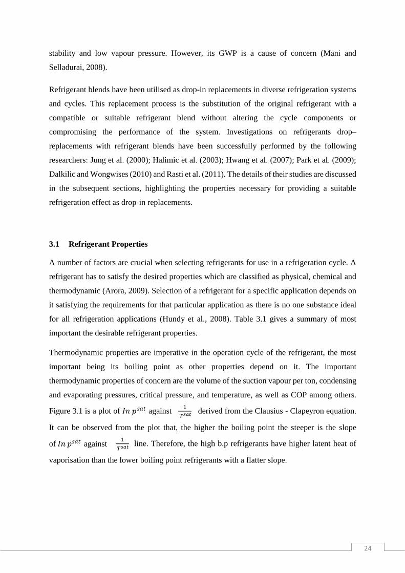
Thermodynamic properties are imperative in the operation cycle of the refrigerant, the most
important being its boiling point as other properties depend on it. The important
thermodynamic properties of concern are the volume of the suction vapour per ton, condensing
and evaporating pressures, critical pressure, and temperature, as well as COP among others.
Figure 3.1 is a plot of 𝐼𝑛 𝑝𝑠𝑎𝑡 against1
𝑇𝑠𝑎𝑡 derived from the Clausius - Clapeyron equation.
It can be observed from the plot that, the higher the boiling point the steeper is the slope
of 𝐼𝑛 𝑝𝑠𝑎𝑡 against1
𝑇𝑠𝑎𝑡 line. Therefore, the high b.p refrigerants have higher latent heat of
vaporisation than the lower boiling point refrigerants with a flatter slope.

25
Figure 3-1 : Comparison of Pressures of Lower Boiling and Higher Boiling Refrigerants at
given Evaporator and Condenser Temperature. (Extracted from Arora, 2009).
Moreover, at a fixed temperature, the condenser and evaporator pressure are lower for higher
boiling temperature refrigerants. Conversely, higher-pressure refrigerants boil at a lower
temperature. Furthermore, the high boiling refrigerants have a higher-pressure ratio while low
boiling refrigerants have lower pressure ratios.
26
Table 3-1 : Summarised Properties of an ideal Refrigerant (Compiled from Arora, 2009;
Sapali, 2009; Mohanraj et al., 2011).
Property Description Specification
Thermodynamic
Ozone Depleting Potential
Global Warming Potential
Latent heat of evaporation
Critical pressure
Critical temperature
Condensing pressure
Evaporating pressure
Zero
Zero
High
High
High
High
Relatively low
Chemical
Toxicity
Flammability
Corrosiveness
Miscibility with oil
Miscibility with water/moisture
Non-toxic
Non-flammable
Non-corrosive
Low
Low
Physical
Leak detection
Cost and availability
Heat transfer coefficient
Viscosity
Thermal conductivity
Dielectric strength
Easy
Cheap and available
High
Low
High
Compatible with air,
refrigerants, and motor
windings
A special emphasis on chemical miscibility with the lubricating oil is that chlorine-based
refrigerant blends mix perfectly with mineral oil. However, HFC refrigerant blends are not
miscible with mineral oil and require synthetic lubricants (Mohanraj et al., 2011). The synthetic
lubricates in use are Polyol ester oil (POE) and alkyl benzene (AB).
27
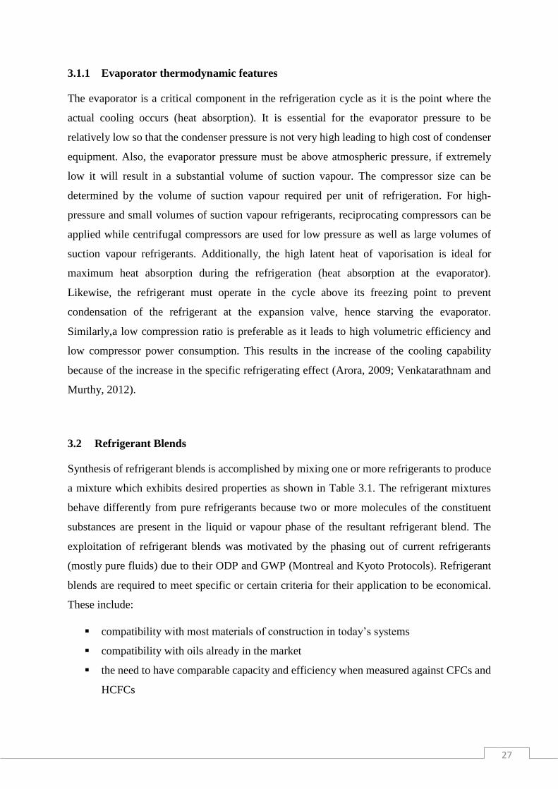
3.1.1 Evaporator thermodynamic features
The evaporator is a critical component in the refrigeration cycle as it is the point where the
actual cooling occurs (heat absorption). It is essential for the evaporator pressure to be
relatively low so that the condenser pressure is not very high leading to high cost of condenser
equipment. Also, the evaporator pressure must be above atmospheric pressure, if extremely
low it will result in a substantial volume of suction vapour. The compressor size can be
determined by the volume of suction vapour required per unit of refrigeration. For high-
pressure and small volumes of suction vapour refrigerants, reciprocating compressors can be
applied while centrifugal compressors are used for low pressure as well as large volumes of
suction vapour refrigerants. Additionally, the high latent heat of vaporisation is ideal for
maximum heat absorption during the refrigeration (heat absorption at the evaporator).
Likewise, the refrigerant must operate in the cycle above its freezing point to prevent
condensation of the refrigerant at the expansion valve, hence starving the evaporator.
Similarly,a low compression ratio is preferable as it leads to high volumetric efficiency and
low compressor power consumption. This results in the increase of the cooling capability
because of the increase in the specific refrigerating effect (Arora, 2009; Venkatarathnam and
Murthy, 2012).
3.2 Refrigerant Blends
Synthesis of refrigerant blends is accomplished by mixing one or more refrigerants to produce
a mixture which exhibits desired properties as shown in Table 3.1. The refrigerant mixtures
behave differently from pure refrigerants because two or more molecules of the constituent
substances are present in the liquid or vapour phase of the resultant refrigerant blend. The
exploitation of refrigerant blends was motivated by the phasing out of current refrigerants
(mostly pure fluids) due to their ODP and GWP (Montreal and Kyoto Protocols). Refrigerant
blends are required to meet specific or certain criteria for their application to be economical.
These include:
▪ compatibility with most materials of construction in today’s systems
▪ compatibility with oils already in the market
▪ the need to have comparable capacity and efficiency when measured against CFCs and
HCFCs
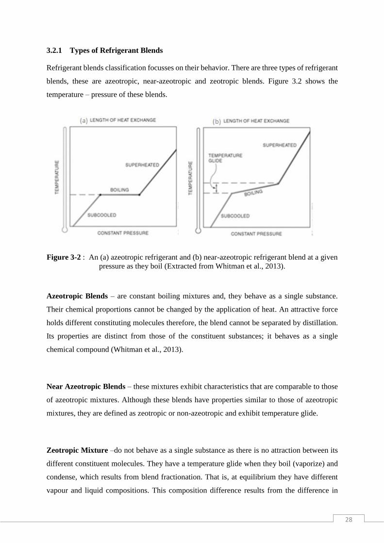
28
3.2.1 Types of Refrigerant Blends
Refrigerant blends classification focusses on their behavior. There are three types of refrigerant
blends, these are azeotropic, near-azeotropic and zeotropic blends. Figure 3.2 shows the
temperature – pressure of these blends.
Figure 3-2 : An (a) azeotropic refrigerant and (b) near-azeotropic refrigerant blend at a given
pressure as they boil (Extracted from Whitman et al., 2013).
Azeotropic Blends – are constant boiling mixtures and, they behave as a single substance.
Their chemical proportions cannot be changed by the application of heat. An attractive force
holds different constituting molecules therefore, the blend cannot be separated by distillation.
Its properties are distinct from those of the constituent substances; it behaves as a single
chemical compound (Whitman et al., 2013).
Near Azeotropic Blends – these mixtures exhibit characteristics that are comparable to those
of azeotropic mixtures. Although these blends have properties similar to those of azeotropic
mixtures, they are defined as zeotropic or non-azeotropic and exhibit temperature glide.
Zeotropic Mixture –do not behave as a single substance as there is no attraction between its
different constituent molecules. They have a temperature glide when they boil (vaporize) and
condense, which results from blend fractionation. That is, at equilibrium they have different
vapour and liquid compositions. This composition difference results from the difference in

29
boiling point of the constituent substances in the mixture. When the mixture boils, due to the
existence of substances with different boiling points there is composition change of the mixture
changing in phase. The composition changes lead to changes in the bubble (Tbub) and the dew
(Tdew) points of the residual mixture.
3.2.2 Behavior of Blends
Temperature glide – is the difference between the dew point temperature and the bubble point
temperature (TG= Tdew – Tbub). It occurs when at a given pressure, the blends have a range of
evaporating and condensing temperatures. A temperature glide occurs because the phase
change takes place at a different pressure-temperature relationship for each component in the
blend. Phase changes occur along the length of the vessel or heat exchanger; this gives rise to
a range of boiling or condensing points for each pressure. Figure 3.2 illustrates the temperature
glide for a near azeotropic blend. Refrigerant blends with a temperature glide (of approximately
5 0C or larger) have the potential of improving the performance and the energy efficiency of
vapour compression system through a process known as temperature glide matching. A full
discussion of temperature glide matching is included in Appendix A along with the effects of
phase change of zeotropic blends on heat transfer coefficients (HTC).
Blend Fractionation – this is the change in the composition of the refrigerant blend due to
preferential vapourisation of the more volatile component in the blend or preferential
condensation of the less volatile component. Also, leakage of one component from the
refrigeration cycle to the environment at a faster rate than the other components in the blend
causes fractionation. The difference in leakage rate is caused by different partial pressures of
each constituting substance in the blend (Lavelle, 2006).
3.3 Review of the Performances of Refrigerants and Refrigerant Blends
Table 3.2 provides a summary of the performance of different refrigerant blends relative to
pure refrigerants as presented in various literature sources, as published over the years of study
in air-conditioning and refrigeration. The comparative study also pays attention to studies
which were both theoretically and experimentally executed.

30
Table 3-2: A Review of Studies published on Refrigerants and Refrigerant Blends. Reference Refrigerant Studied Application/Method for Study Results and Conclusions Comments
(Rigola et al.,
1996) and
(Rigola et al.,
1998)
R12, R290a, R600a,
R404a, and R134a
An experimental unit was built to
compare the results obtained from
the numerical simulations with the
experimental data. Working on a
single-stage vapour compression
refrigerant scheme, mass flow rate,
and inlet temperature were
independently fixed in the
secondary condenser and evaporator
circuits.
In the theoretical study the COP values for the
refrigerants R134a, R12 and R290 were 1.69, 1.58 and
1.55 respectively. In the experimental runs refrigerants
R134a, R600a, and R404a were studied, and their COP
values were 1.57, 1.49 and 1.18.
Considering refrigerant R134a
which was used both in the
theoretical and experimental
studies, it is observable that the
COP values obtained in the
investigation were comparable.
(Jung et al.,
2000)
Refrigerant blends
made from
refrigerants, R22,
R32, R125, R134a,
R152a, R290, and
R1270
Investigation of the performance of
14 refrigerant mixtures. The
experimental set up consisted of a
simple vapour compression cycle
(VCC) composed of a suction line
heat exchanger, a condenser, an
evaporator and an expansion valve
COPs and refrigeration capacities of three refrigerants
consisting of R125, R32, and R134a were 4-5% higher
than those of R22. Blends with a greater mass fraction
of R32 and R134a and a lower mass fraction of R125
proved to have better performance than R407C. COP
increased to a maximum of 3.9% for mixtures with high
quantities of R125. The COP values for the refrigerant
blends investigated were in the range of 2.339 to 2.660,
with (75%R125/5%R134a/20%R152a) blend having
the lowest value and (26%R32/14%R125/60%R134a)
had the highest value for COP and relatively a high
discharge temperature.
The use of suction line heat
exchanger (SLHX) increased the
COPs of most refrigerants tested
however it lowered their
capacity. Furthermore, from the
results published in this study, it
can be established that increasing
the percentage of R125 in the
blend decreased the COP of the
blend.

31
Table 3-2: A Review of Studies published on Refrigerants and Refrigerant Blends. (Continued) Reference Refrigerant Studied Application/Method for Study Results and Conclusions Comments
(Halimic et al.,
2003)
R12, R134a R401,
and R290
Experimental work carried out in
vapour compression refrigeration
unit originally designed to operate
with R12
R290 had the largest cooling capacity. COP of R12.
R290 and R134a are shown to be comparable. With
regards to environmental effect, R290 showed the best
performance. R401 displayed a level of performance
like that of R12 in both COP and capacity.
Satisfactory performance was
shown by refrigerant blend R401
in the vapour system of
refrigerant R12.
(Hwang et al.,
2004)
R290, R410a, R404a The environmental impact of the
refrigerant blend is of paramount
importance in selecting refrigerant
for use. Lifecycle climate analysis
performance on the given
refrigerants for low and medium
temperature applications.
The COP of R410a is almost the same as that of R290
within the measurement error range, while the COP of
R404a is 5-10% lower than that of R290. Also, the
LCCP of R290 is always lower than that of R410a and
R404a if the annual emission is kept below 10%,
therefore, it is conclusive that HCs have lower LCCP
than HFCs.
As far as environmental aspects
were concerned which are
summarised by LCCP analysis,
R404a and R410a exhibited
better performance than R290.
(Wongwises et
al., 2006)
Refrigerant blends
made from, R134a,
R290, R600, and
R600a.
Investigated the performance of
blends in an Automobile air
conditioning, with a capacity of 3.5
kW driven by a diesel engine.
Parameters evaluated were
compressor power, refrigeration
capacity and COP.
Every blend composition had a larger COP than R134a,
lower discharge temperature, however the capacity was
comparable. The blend R290/R600/R600a in the ratio
(50%/40%/10%) had the highest COP in all the tested
conditions. At compressor speed of 1500 rpm,
evaporator temperature of 5 ℃, COP for
R290/R600/R600a in the ratio (50%/40%/10%) was
1.55 while that for R134a was 1.33 Hence it is the best
alternative to R134a.
The hydrocarbon blends
exhibited excellent refrigeration
capabilities in the study with
regards to COP, compressor
power, and the cooling capacity.
The performance of the
refrigerant blends was
satisfactory in the automobile air
conditioning designed for use
with pure refrigerants.

32
Table 3-2: A Review of Studies published on Refrigerants and Refrigerant Blends. (Continued)
Reference Refrigerant Studied Application/Method for Study Results and Conclusions Comments
(Mani and
Selladurai, 2008)
R12, R134a, and
R290/R600a
Experimental performance of the
refrigerants was investigated in a
vapour compression refrigeration
system originally designed to
operate with R12. Investigations
were carried out at various
evaporating temperatures between -
2 and 18 ℃.
Refrigerant mixture R290/R600a in the ratio (68/32 by
wt %) showed the best performance with regards to
major environmental impacts (ODP) and GWP). The
blend had comparable discharge temperature and
pressure with R134a and R12.
In this study, the hydrocarbon
blend showed better performance
than pure refrigerants used in the
study. It can also be drawn from
the study that different
refrigerant mixture compositions
behave differently in different
proportions.
(Dalkilic and
Wongwises,
2010)
R12, R134a, R134a,
R152a, R32, R290,
R1270, R600 and
R600a.
A theoretical study of a VCRC was
carried out with various refrigerant
blends at different ratios, the
parameters of interest were the COP,
degree of superheating and sub-
cooling, the refrigeration effect, the
environmental impacts of ozone
layer depletion and global warming.
Refrigerant blends R290/R600a (40/60 by wt %) and
R290/R1270 (20/80 by wt %) with COP values of 2.893
and 3.180, were found to be most suitable replacements
for R12 and R22 respectively. The COP value obtained
for R134a was 3.097 while for R12 it was 3.233, with
the condenser temperature set at 50 ℃ and the
evaporator temperature at -10 ℃.
Satisfactory performance of the
refrigerant blends in the
theoretical analyses carried out in
this study.
(Padilla et al.,
2010)
R12 and R413a Investigation of Exergy
performance of the two refrigerants
in the domestic refrigeration system.
Refrigerant R413 showed better performance than R12,
the COP value for R413 was 3.72 while that of R12 was
3.53.
R413a exhibited excellent
refrigeration performance,
exergy efficiency and ozone
friendly therefore a safe, viable
alternative to R12. R413a can be
used to replace R12 with little or
no system’s modification.

33
Table 3-2: A Review of Studies published on Refrigerants and Refrigerant Blends. (Continued)
Reference Refrigerant Studied Application/Method for Study Results and Conclusions Comments
(Jain et al., 2011) R22, R134a, R410A,
R407C, and M20
COP computation by a simulation
program (RERPROF) based on the
following input data: evaporator
coolant inlet temperature, condenser
coolant inlet temperature, the rate of
heat absorbed by the evaporator, the
efficiency of the compressor, and
product evaporator (and condenser)
effectiveness and capacitance rate of
the external fluid.
The COP value obtained for R134a was 2.31, while the
compressor work was 28.92 kW with the refrigerant
flow rate of 0.535 kg/s. The COP value of R22, R410a,
R407C and M20 was 2.35, 2.06, 2.33 and 2.18
respectively. Their compressor work (kW) was 28.25,
32.34, 28.63 and 30.54 respectively.
From the comparisons made, it
was conclusive that R407C was
the potential HFC refrigerant for
new and existing systems using
R22 with minimum costs and
human efforts.
(Bolaji, 2011) R22, R507, and
R404A
Window air-conditioner application.
R22 was used as a benchmark to
assess the performance of the two
refrigerant blends. COP, pressure
ratios, compressor power.
Refrigeration capacity and
discharge temperature were the
parameters investigated.
R507 had a high COP value compared to that for the
other refrigerants studied. The COP of the refrigerants
R22, R507 and R404a were 2.07, 2.19 and 2.93
respectively and the compressor work (kW) was 1.86,
1.83 and 1.90 respectively. While the discharge
temperatures (℃) 47.5, 49.4 and 54.6 respectively.
The study proved the excellent
refrigeration performance of the
refrigerant blends as their
performance was better than that
of the pure refrigerant used in the
study.
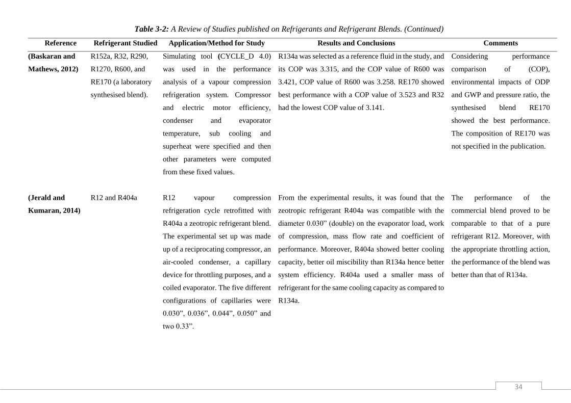
34
Table 3-2: A Review of Studies published on Refrigerants and Refrigerant Blends. (Continued)
Reference Refrigerant Studied Application/Method for Study Results and Conclusions Comments
(Baskaran and
Mathews, 2012)
R152a, R32, R290,
R1270, R600, and
RE170 (a laboratory
synthesised blend).
Simulating tool (CYCLE_D 4.0)
was used in the performance
analysis of a vapour compression
refrigeration system. Compressor
and electric motor efficiency,
condenser and evaporator
temperature, sub cooling and
superheat were specified and then
other parameters were computed
from these fixed values.
R134a was selected as a reference fluid in the study, and
its COP was 3.315, and the COP value of R600 was
3.421, COP value of R600 was 3.258. RE170 showed
best performance with a COP value of 3.523 and R32
had the lowest COP value of 3.141.
Considering performance
comparison of (COP),
environmental impacts of ODP
and GWP and pressure ratio, the
synthesised blend RE170
showed the best performance.
The composition of RE170 was
not specified in the publication.
(Jerald and
Kumaran, 2014)
R12 and R404a R12 vapour compression
refrigeration cycle retrofitted with
R404a a zeotropic refrigerant blend.
The experimental set up was made
up of a reciprocating compressor, an
air-cooled condenser, a capillary
device for throttling purposes, and a
coiled evaporator. The five different
configurations of capillaries were
0.030”, 0.036”, 0.044”, 0.050” and
two 0.33”.
From the experimental results, it was found that the
zeotropic refrigerant R404a was compatible with the
diameter 0.030” (double) on the evaporator load, work
of compression, mass flow rate and coefficient of
performance. Moreover, R404a showed better cooling
capacity, better oil miscibility than R134a hence better
system efficiency. R404a used a smaller mass of
refrigerant for the same cooling capacity as compared to
R134a.
The performance of the
commercial blend proved to be
comparable to that of a pure
refrigerant R12. Moreover, with
the appropriate throttling action,
the performance of the blend was
better than that of R134a.
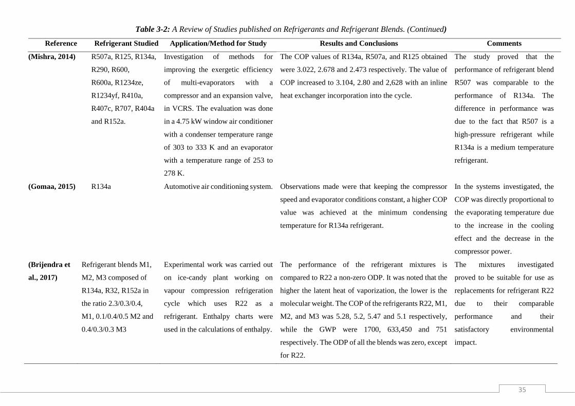
35
Table 3-2: A Review of Studies published on Refrigerants and Refrigerant Blends. (Continued)
Reference Refrigerant Studied Application/Method for Study Results and Conclusions Comments
(Mishra, 2014) R507a, R125, R134a,
R290, R600,
R600a, R1234ze,
R1234yf, R410a,
R407c, R707, R404a
and R152a.
Investigation of methods for
improving the exergetic efficiency
of multi-evaporators with a
compressor and an expansion valve,
in VCRS. The evaluation was done
in a 4.75 kW window air conditioner
with a condenser temperature range
of 303 to 333 K and an evaporator
with a temperature range of 253 to
278 K.
The COP values of R134a, R507a, and R125 obtained
were 3.022, 2.678 and 2.473 respectively. The value of
COP increased to 3.104, 2.80 and 2,628 with an inline
heat exchanger incorporation into the cycle.
The study proved that the
performance of refrigerant blend
R507 was comparable to the
performance of R134a. The
difference in performance was
due to the fact that R507 is a
high-pressure refrigerant while
R134a is a medium temperature
refrigerant.
(Gomaa, 2015) R134a Automotive air conditioning system. Observations made were that keeping the compressor
speed and evaporator conditions constant, a higher COP
value was achieved at the minimum condensing
temperature for R134a refrigerant.
In the systems investigated, the
COP was directly proportional to
the evaporating temperature due
to the increase in the cooling
effect and the decrease in the
compressor power.
(Brijendra et
al., 2017)
Refrigerant blends M1,
M2, M3 composed of
R134a, R32, R152a in
the ratio 2.3/0.3/0.4,
M1, 0.1/0.4/0.5 M2 and
0.4/0.3/0.3 M3
Experimental work was carried out
on ice-candy plant working on
vapour compression refrigeration
cycle which uses R22 as a
refrigerant. Enthalpy charts were
used in the calculations of enthalpy.
The performance of the refrigerant mixtures is
compared to R22 a non-zero ODP. It was noted that the
higher the latent heat of vaporization, the lower is the
molecular weight. The COP of the refrigerants R22, M1,
M2, and M3 was 5.28, 5.2, 5.47 and 5.1 respectively,
while the GWP were 1700, 633,450 and 751
respectively. The ODP of all the blends was zero, except
for R22.
The mixtures investigated
proved to be suitable for use as
replacements for refrigerant R22
due to their comparable
performance and their
satisfactory environmental
impact.

36
Chapter 4
4 Equipment Review
Laboratory scale refrigerant units are designed and assembled for investigating and analysing
the performance of refrigerants and refrigerant blends. Refrigerant test units are designed and
assembled differently to meet specific and unique experimental requirements. Modifications
are sometimes necessary when refrigerant blends are investigated in a unit originally intended
for pure refrigerants. Additionally, laboratory scale refrigeration units are not novel, but
available pre-constructed, in parts or designed for specific research purposes. The capabilities
of these units are as vast as the interests of the industry today. A literature review of the
equipment used in the laboratory scale refrigeration experimental research is provided in this
chapter.
4.1 Equipment Setups presented in literature
Figure 4-1 : Experimental set-up for R12, R134a, and R290/600a investigation (Extracted
from Mani and Selladurai, 2008).
Mani and Selladurai (2008) performed an experimental study on a vapour compression cycle
on the equipment setup shown in Figure 4.1 constructed for the study. The refrigerants studied

37
were R12, R134a and R290/R600a. Two loops are evident in the setup, the main loop, and the
secondary loop. The compressor, the evaporator, a filter drier, the condenser, sight glass, flow-
meter and expansion valve make up the main refrigeration loop.
The evaporator and the condenser were of double tubes made from copper. In the condenser,
the refrigerant flows in the inside tube whereas the cooling water flows through the annular
space between the interior and exterior tubes. In the evaporator, a calcium chloride solution
was used as a heat transfer fluid, and it flows through the interior tube while the refrigerant
flows in the annular space.
A reciprocating compressor selected for the study had a rotating speed of 855 rpm which could
be adjusted by an electrical motor. The tube and refrigerant lines were insulated to reduce heat
loss. Two sight glasses were included in the unit, one on the liquid line and the other on the
suction line. Cooling water from one tank was circulated through the condenser whereas brine
solution in another tank was circulated through the evaporator. Cooling water from the
condenser was cooled in a cooling tower. Highly sensitive rotameters were utilised to meter
the flow rates of the brine solution and the cooling water, their accuracy was ± 0.05 L/min.
RTD thermocouples were employed to measure the temperature, with an accuracy of ± 0.1 ℃
and the pressure gauges used to measure pressure were calibrated with an accuracy of ± 6.89
kPa.
Jung et al. (2000) in their investigation of potential substitutes for R22 in household air-
conditioners used the breadboard heat pump set-up shown in Figure 4.2. The refrigerant
mixtures tested in the unit were: R32, R125, R290, R1270, R134a and R152a.
The condenser and evaporator were of the double line heat exchanger type designed to have
counter- current flow. The refrigerant fluid flows through the annulus, while the secondary heat
transfer which was water in both the evaporator and condenser flowed in the inner tube. The
temperature of the water was controlled by a chiller and a heater at the condenser and
evaporator respectively. This unit was also used by Park et al. (2009) to prove the suitability
of R413a as a drop-in substitute for R22 in residential air-conditioners and heat pumps.
For pressure changers, a hermetic compressor, designed for use with R22, was installed. A fine
metering valve was used as the expansion valve. To increase the efficiency of the system, an
SLHX was connected. The vapour exiting the evaporator was channelled into the innermost
tube while the liquid from the condenser flowed through the annulus of the SLHX. The unit

38
was insulated by polyurethane and fibreglass to reduce heat loss. Charging ports were at the
evaporator inlet for liquids and the other at the condenser inlet for gases.
Figure 4-2 : The breadboard heat pump (Extracted from Jung et al., 2000).
Halimic et al. (2003) compared the performances of R410, R290, and R134a with R12 in a
vapour compression refrigeration cycle in a test rig designed for R12 refrigerant, using the
equipment set up shown in Figure 4.3. To facilitate the examination of alternative refrigerants,
it was necessary to dismount the temperature sensor at the expansion valve which was
originally intended to optimise system performance with R12 refrigerant. A sight glass
positioned, between the expansion valve and the condenser, in the Halimic et al (2003) unit it
is used to detect the refrigerant phase as it enters the expansion valve. In the test procedure, the
evaporator temperature value was fixed. Other parameters, i.e. the condenser temperature,
cooling water temperature, refrigerant flow rate, condenser and evaporator pressures, were
adjusted to meet the operational conditions. In every experimental run, once stable conditions
were achieved, readings were taken and recorded after an hour of operation. The observations
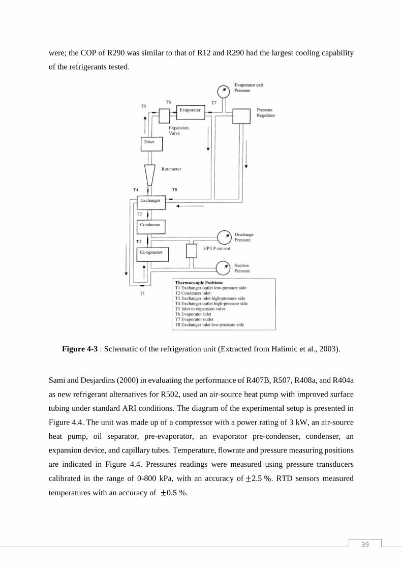
39
were; the COP of R290 was similar to that of R12 and R290 had the largest cooling capability
of the refrigerants tested.
Figure 4-3 : Schematic of the refrigeration unit (Extracted from Halimic et al., 2003).
Sami and Desjardins (2000) in evaluating the performance of R407B, R507, R408a, and R404a
as new refrigerant alternatives for R502, used an air-source heat pump with improved surface
tubing under standard ARI conditions. The diagram of the experimental setup is presented in
Figure 4.4. The unit was made up of a compressor with a power rating of 3 kW, an air-source
heat pump, oil separator, pre-evaporator, an evaporator pre-condenser, condenser, an
expansion device, and capillary tubes. Temperature, flowrate and pressure measuring positions
are indicated in Figure 4.4. Pressures readings were measured using pressure transducers
calibrated in the range of 0-800 kPa, with an accuracy of ±2.5 %. RTD sensors measured
temperatures with an accuracy of ±0.5 %.
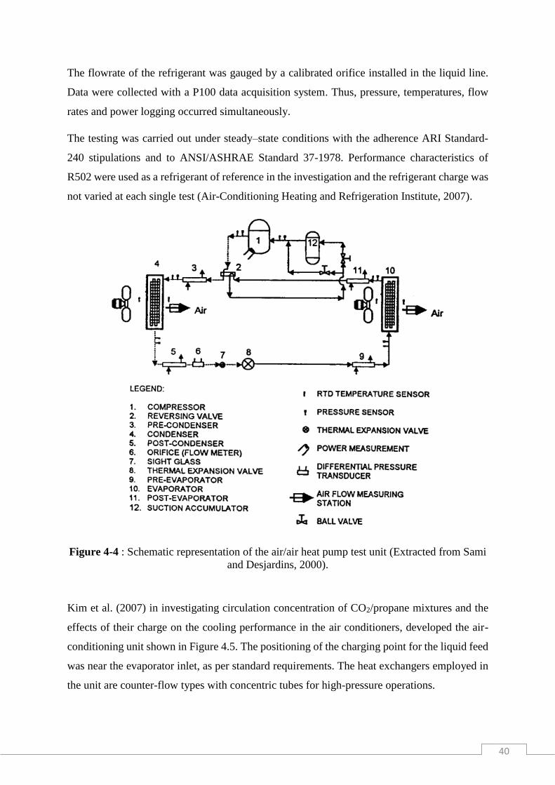
40
The flowrate of the refrigerant was gauged by a calibrated orifice installed in the liquid line.
Data were collected with a P100 data acquisition system. Thus, pressure, temperatures, flow
rates and power logging occurred simultaneously.
The testing was carried out under steady–state conditions with the adherence ARI Standard-
240 stipulations and to ANSI/ASHRAE Standard 37-1978. Performance characteristics of
R502 were used as a refrigerant of reference in the investigation and the refrigerant charge was
not varied at each single test (Air-Conditioning Heating and Refrigeration Institute, 2007).
Figure 4-4 : Schematic representation of the air/air heat pump test unit (Extracted from Sami
and Desjardins, 2000).
Kim et al. (2007) in investigating circulation concentration of CO2/propane mixtures and the
effects of their charge on the cooling performance in the air conditioners, developed the air-
conditioning unit shown in Figure 4.5. The positioning of the charging point for the liquid feed
was near the evaporator inlet, as per standard requirements. The heat exchangers employed in
the unit are counter-flow types with concentric tubes for high-pressure operations.

41
The inclusion of the oil separator in the unit was prompted by the fact that the thermodynamic
interactions of the oil and refrigerant were not known. The unit was equipped with instruments
to gauge pressure, temperature, circulation concentration, mass flow rate, and compressor
power. To measure the concentration of propane/carbon dioxide in the circulation, refrigerant
mixture samples were taken in liquid and gas form from the liquid receiver and evaporator
outlet respectively. Gas chromatography analysed samples in adherence to the standards of
ANSI/ASME, (Air-Conditioning Heating and Refrigeration Institute, 2007).
Figure 4-5 : Schematic of the experimental setup for the performance test of CO2/propane
mixture (Extracted from Kim et al., 2007).
Chesi et al. (2012) designed and assembled a refrigeration test rig to investigate the
performance of R744 in several cycle layouts. The unit comprised a complete vapour
compression cycle with the addition of inter-coolers, economizers and an internal heat
exchanger (Figure 4.6) rated up to 14 MPa. The piping and valve network allows for the
individual system components to be bypassed and incorporate external components, thus
increasing system versatility. Data acquisition software records the following measurements
temperature, power, pressure, and mass flow rate.
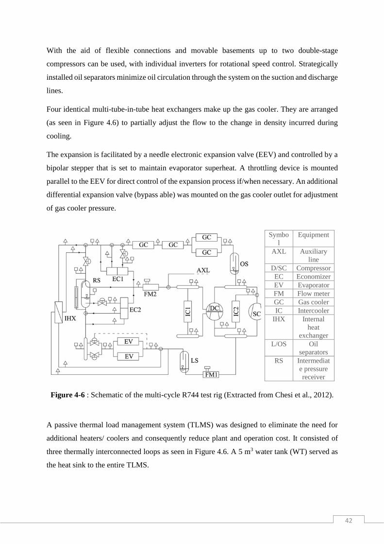
42
With the aid of flexible connections and movable basements up to two double-stage
compressors can be used, with individual inverters for rotational speed control. Strategically
installed oil separators minimize oil circulation through the system on the suction and discharge
lines.
Four identical multi-tube-in-tube heat exchangers make up the gas cooler. They are arranged
(as seen in Figure 4.6) to partially adjust the flow to the change in density incurred during
cooling.
The expansion is facilitated by a needle electronic expansion valve (EEV) and controlled by a
bipolar stepper that is set to maintain evaporator superheat. A throttling device is mounted
parallel to the EEV for direct control of the expansion process if/when necessary. An additional
differential expansion valve (bypass able) was mounted on the gas cooler outlet for adjustment
of gas cooler pressure.
Symbo
l
Equipment
AXL Auxiliary
line
D/SC Compressor
EC Economizer
EV Evaporator
FM Flow meter
GC Gas cooler
IC Intercooler
IHX Internal
heat
exchanger
L/OS Oil
separators
RS Intermediat
e pressure
receiver
Figure 4-6 : Schematic of the multi-cycle R744 test rig (Extracted from Chesi et al., 2012).
A passive thermal load management system (TLMS) was designed to eliminate the need for
additional heaters/ coolers and consequently reduce plant and operation cost. It consisted of
three thermally interconnected loops as seen in Figure 4.6. A 5 m3 water tank (WT) served as
the heat sink to the entire TLMS.

43
The temperature of the (50/50) water/ ethylene glycol stream that provides the heat duty to the
evaporator was maintained by heat transfer (HX2) with the water circulating through the gas
cooler. To balance the heat duties for this process, a portion of the gas cooler water is first pre-
cooled in HX1. The set of valves denoted by circles in Figure 4.7 allowed for two different
TLMS configurations that facilitate different temperature ranges for the evaporator and gas
cooler. Both heat exchangers were fitted with bypass lines and mixing valves for varying
temperatures. These temperatures were maintained by thermostatic PI control of the respective
mixing valves. A numerical model was developed to approximate the limitations and
performance of the TLMS.
Symbol Equipment
EV Evaporator
GC Gas cooler
HX Heat
exchanger
R1/ R2 Receivers
WT Water tank
Figure 4-7 : Layout of the thermal load management system (Extracted from Chesi et al.,
2012).
The effect of adding an inner heat exchanger (IHX) to a single stage system was also reperted
in the study. Experiments were carried out at suction pressures of 2.6 and 3.3 MPa and gas
cooler pressures in the range of 6 to 12 MPa (for water outlet temperatures corresponding to
20, 30 and 40 ℃). Evaporator pressure and suction superheat were controlled by adjustment of
the expansion valve and variation of evaporator HTF temperature respectively. Gas cooling
pressure and outlet R744 temperature were controlled by adjustment of the differential
expansion valve and variation of the HTF temperature.
Presented in this chapter are published refrigerant equipment which were used in various
laboratory experimental investigations of refrigeration applications. In designing the
refrigerant unit utilised for this study, essential technical details stated in the publications were
44
incorporated and some improvements were crucial due to a number of cycles which were to be
operated on the unit. As previously discussed, the properties of different refrigerants are such
that they place many restrictions on the units for which they are designed, the majority of which
are only economically operable with the design refrigerant.
In the test rig developed for this study, the positioning of critical components such as sight
glasses and filter dryers in this study was in line with specifications outlined in this preview.
The refrigerant unit was designed to operate in a number of cycles which are simple vapour -
compression cycle, two-stage vapour compression cycle, cascade system, vapour compression
cycle with a suction-line heat exchange. Also, the test rig can be used for the investigation of
the following refrigerants and refrigerant blends, R134a, R22, R404a, R407C, R407F, R410a
or R507a as per filter dryer specifications and refrigerants R134a, R404a, R407A/C/F, and
R507a as these are compatible with the compressor oil. Moreover, there are limitations due to
temperature and pressure pertaining to the unit’s operation range, these being 100 ℃ and 1.9
MPa respectively.
45
Chapter 5
5 Equipment Description
This chapter presents the original design of the test unit, the description, and specifics of each
component in the unit and the modifications carried out.
The refrigeration test rig used in this study was designed and built in the Thermodynamics
Research Unit by a MSc. Eng. student, Ms. Alisha Kate Shadrach, under the supervision of
Professors J.D Raal, P Naidoo, and D Ramjugernath. The unit was designed in the year 2012.
Although the unit was assembled during 2014, it was not commissioned. Calibration of sensors
and pressure tests were carried out soon after the construction phase however, Shadrach did
not overcome the issues of sealing in achieving very low pressures/desired level of vacuum
required in the refrigeration unit.
During the initial part of this study, the need for major modifications were identified and as
such changes had to be made to the equipment design and construction. These modifications
are discussed in section 5.7 which included overcoming the sealing problems encountered in
the unit which were mainly due to leaks in the condenser seals, vibration eliminators and in a
number of loose joints in the unit. Furthermore, to achieve the throttling effect the metering
valves were removed due to their small orifice which was a hindrance to the passage of the
liquid refrigerant to the expansion valve. There was also a need to replace water baths at the
condenser and evaporator with larger ones to meet the duties of these two heat exchangers.
5.1 Original Design
The refrigeration unit was intended to be utilised in evaluating the performance of the existing,
potential and alternative refrigerants and refrigerant blends for refrigeration application. In this
study, the experimental measurements were carried out in a simple vapour -compression cycle.
Additionally, the test rig can also be configured into the following different cycles:
• Two stage Vapour – Compression Cycle
• Cascade System
• Vapour –Compression Cycle with a Suction-line Heat Exchanger
The presentation of the schematic design of the original refrigeration unit is shown in Figure
5.1. The unit has three main parts: the low-pressure (LP) section: the data acquisition section
and the high pressure (HP) section. The LP section contains an evaporator (EV-01); the HP

46
section houses a condenser (CN-01) and; the data acquisition system has a cRIO (Compact
Reconfigurable Input and Output unit). The unit has two compressors for use in the cascade
cycle and two-stage vapour compression cycle. The components of the units and their
specifications are listed below:
• a suction line heat exchanger: 3.5 kW capacity B3-012-28-H brazed plate heat exchangers
• an evaporator: 2.5 kW capacity B3-012-14-H brazed plate heat exchangers
• a condenser: 3.82 kW capacity B3-027-16-H brazed-plate heat exchangers
• two semi-hermetic reciprocating Bitzer 2KES-05(Y) compressors (each with a compressor
control panel),
• two Danfoss VLT Microdrive for motor frequency control,
• two Afcon Industrial Equipment Heldon oil separators,
• two Afcon Industrial Equipment Heldon suction accumulators,
• two Afcon Industrial Equipment liquid receivers,
• two water baths (10 litres and 34 litres),
• two Elepon-seal-less SL-10S 0.1 kW, 220 V (centrifugal) liquid pumps,
• two 1-10 L/min Ximatrix water rotameters, bottom/top entry brass,
• two SAD-163 solid core liquid line filter driers,
• two ¼ flares KSG2MF liquid line sight glass moisture indicators,
• two Swagelok SS-4MG-BU-MH, 0.0056inch/1.42mm metering valves,
• two Swagelok SS-4L-BU-MH, 0.128inch/3.25mm orifice expansion valves,
• two variable frequency drives (VLTs) (one for each compressor), and
• multiple two ports and three port Swagelok valves,
• nine WIKA A-10 pressure transmitters
• eleven WIKA T1TEBTSS15 temperature thermocouples,
• A network of copper and stainless pipes that connect the components in the unit.
• two Grant TX150 digital temperature controller
• two PolyScience flow through chillers model KR-80A
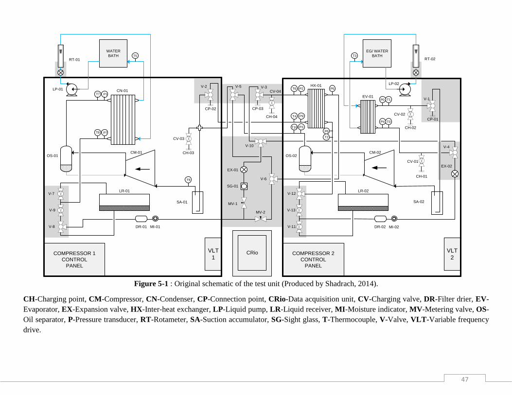
47
VLT
1
VLT
2COMPRESSOR 2
CONTROL
PANEL
COMPRESSOR 1
CONTROL
PANEL
CN-01
HX-01
EV-01
V-5
V-10
V-1
V-4
EX-02EX-01
SG-01
CP-01
CP-03
T2
T1
T6
SA-01 SA-02
OS-02
V-6
V-2
V-12
MI-01
LR-01
MI-02
LR-02
MV-2
V-3
V-8
CH-02
CH-03
CH-04
CH-01
CP-02
V-11
V-13V-9
CV-03
CV-04
CV-01
P0
P2
P6
T0P4
CV-02
T10 P3
T4 P9
T7 P1
P5
DR-01
V-7
DR-02
T8 P7
MV-1
WATER
BATH
EG/ WATER
BATHT3
OS-01
T9
CM-02CM-01
T5
CRio
LP-01
LP-02
RT-01 RT-02
Figure 5-1 : Original schematic of the test unit (Produced by Shadrach, 2014).
CH-Charging point, CM-Compressor, CN-Condenser, CP-Connection point, CRio-Data acquisition unit, CV-Charging valve, DR-Filter drier, EV-
Evaporator, EX-Expansion valve, HX-Inter-heat exchanger, LP-Liquid pump, LR-Liquid receiver, MI-Moisture indicator, MV-Metering valve, OS-
Oil separator, P-Pressure transducer, RT-Rotameter, SA-Suction accumulator, SG-Sight glass, T-Thermocouple, V-Valve, VLT-Variable frequency
drive.

48
5.2 Refrigerant Cycles in the Test rig
Schematic representations and descriptions of each refrigeration cycle configuration possible in
the unit are detailed in Appendix C.
5.3 General Unit Description
The refrigeration unit comprises of four charging points, labeled CH (charging point) as shown in
Figure 5.1. These ports were used to introduce the refrigerant into the unit. CH-01 and CH-04 were
liquid refrigerant inlets located in the liquid line, while gaseous refrigerant charging ports CH-02
and CH-03 were located on the suction line.
5.3.1 Piping
Copper and stainless-steel pipes commonly used in air-conditioning and refrigeration systems,
were used as refrigerant pipelines in the unit. Metal pipes are named after their internal pipe
diameters. In this unit, ⅝” (⅝ inch), ⅜” (⅜ inch), ⅛” (⅛ inch), ¼” (¼ inch), ½” (½ inch) pipes
were used for refrigerant pipeline in the test rig. These pipes were insulated with nitrile rubber
insulation, of Armaflex class O type, to exclude the environmental influence on the system.
The ½” copper pipe was used as the compressor suction lines and in linking the oil separators and
the compressor. In these sections, the refrigerant was in the vapour phase.
The ⅛” stainless steel pipes are the smallest in diameter when compared to the other pipes fixed
in the unit. These pipes were fitted in between the pressure tap-off points and the pressure
transducers.
The use of ⅜” copper pipe was extensive in the unit. It was mainly utilised in the transportation of
the liquid-vapour refrigerant mixtures. Primarily, the ⅜” line was used to convey the compressed
gas from the compressor to the condenser; and to carry the refrigerant from the oil separator, i.e.,
OS-02 to valve 6 (refer to Figure 5.1). Also, it was installed at the heat exchanger outlet, via P2
and T6 through V-3, and then to V-10, where the pipe branched: one end led to EX-01 and the
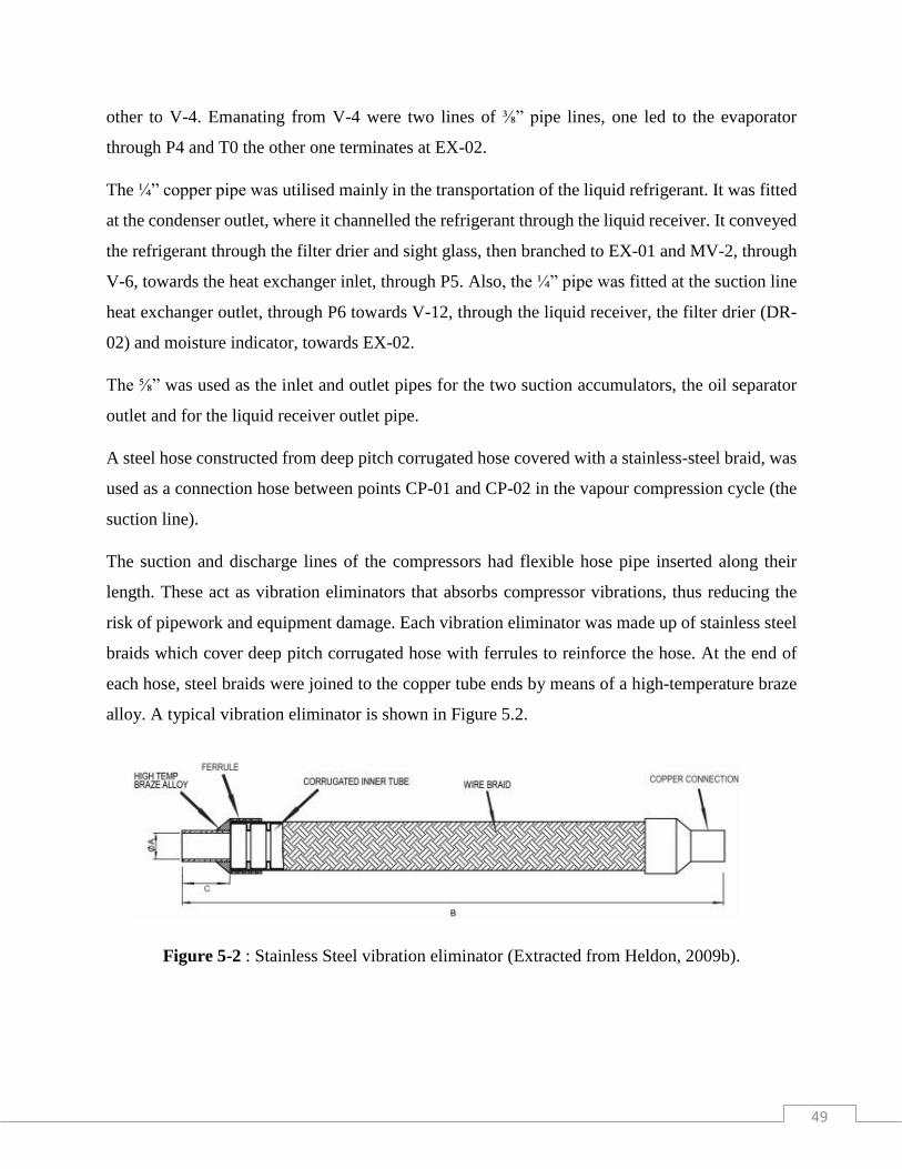
49
other to V-4. Emanating from V-4 were two lines of ⅜” pipe lines, one led to the evaporator
through P4 and T0 the other one terminates at EX-02.
The ¼” copper pipe was utilised mainly in the transportation of the liquid refrigerant. It was fitted
at the condenser outlet, where it channelled the refrigerant through the liquid receiver. It conveyed
the refrigerant through the filter drier and sight glass, then branched to EX-01 and MV-2, through
V-6, towards the heat exchanger inlet, through P5. Also, the ¼” pipe was fitted at the suction line
heat exchanger outlet, through P6 towards V-12, through the liquid receiver, the filter drier (DR-
02) and moisture indicator, towards EX-02.
The ⅝” was used as the inlet and outlet pipes for the two suction accumulators, the oil separator
outlet and for the liquid receiver outlet pipe.
A steel hose constructed from deep pitch corrugated hose covered with a stainless-steel braid, was
used as a connection hose between points CP-01 and CP-02 in the vapour compression cycle (the
suction line).
The suction and discharge lines of the compressors had flexible hose pipe inserted along their
length. These act as vibration eliminators that absorbs compressor vibrations, thus reducing the
risk of pipework and equipment damage. Each vibration eliminator was made up of stainless steel
braids which cover deep pitch corrugated hose with ferrules to reinforce the hose. At the end of
each hose, steel braids were joined to the copper tube ends by means of a high-temperature braze
alloy. A typical vibration eliminator is shown in Figure 5.2.
Figure 5-2 : Stainless Steel vibration eliminator (Extracted from Heldon, 2009b).
50
5.4 Component Specification
5.4.1 Expansion Valve
The throttling devices used in the test rig were Swagelok fine metering valves. These pressure
changers were manually operated valves, i.e., they were hand adjusted depending on the system’s
load. The valve was a screw down, needle valve, designed to provide fine adjustments (McGeorge,
1998). The properties of the valves are given in Table B.2 in Appendix B.
In the hand-operated valve, the change in diameter in the flow pipe gives resistance to the liquid,
which provides the needed pressure drop in the refrigerant flow. In this case, the maximum orifice
of the throttling valve was 0,128 inches (3.25 mm).
In the original design of the unit, a metering valve was placed before the throttling valve with the
purpose of metering the refrigerant flow and regulating the amount of refrigerant passing through
to the expansion valve. The metering valve was hand-operated, with the same specifications as the
expansion valve: its maximum orifice was 0.0056 inch/1.42 mm. It was placed at the high-pressure
section of the flow. In the experimental runs, the expansion valve was set at either a fully open
position or the half open position.
5.4.2 Heat Exchangers
Three brazed-plate heat exchangers acquired from MIT Smart solution perfect systems (in Turkey)
were used as the condenser, the evaporator, and the suction line heat exchanger in the unit. The
specifications of these units are provided in Table 5.1. This type of heat exchanger was selected
because of its compactness and efficient performance in refrigeration applications (Hesselgreaves,
2011).
Plate Heat Exchanger
The plate heat exchangers (PHE), consist of a stack of corrugated or pressed metal plates in mutual
contact for effective heat exchange by fluid spreading evenly over the plates. Inlet and outlet ports
are positioned at the four corners and their seals designed to direct the fluids in other flow passages.
The fluids flow in spaces between the adjacent plates which enables the two flowing streams in

51
adjoining plates to exchange heat as shown in Figure 5.3. The flow pattern shown is referred to as
a single pass counter-current of the U-arrangement type.
Figure 5-3: Flow diagram of a single-pass counter flow arrangement (Extracted from Kakac et
al., 2012).
5.4.3 Evaporator
Water and the refrigerant were the two fluids which flowed counter-current through the evaporator.
The liquid-gas mixture, which entered the evaporator, existed in the gaseous form after it gained
heat energy from water at a higher temperature, in alternate plates. The evaporator was insulated
from the surroundings with nitrile rubber of armaflex class O type.
5.4.4 Condenser
Water and the refrigerant were the two fluids which flowed counter-current through the condenser.
The refrigerant entered in a gaseous state and existed in the liquid state. The heat discarded by the
refrigerant was evident in the temperature increment of water as it exited the condenser. To
eliminate heat exchange with the atmosphere, fiberglass cloth was wrapped around the condenser.
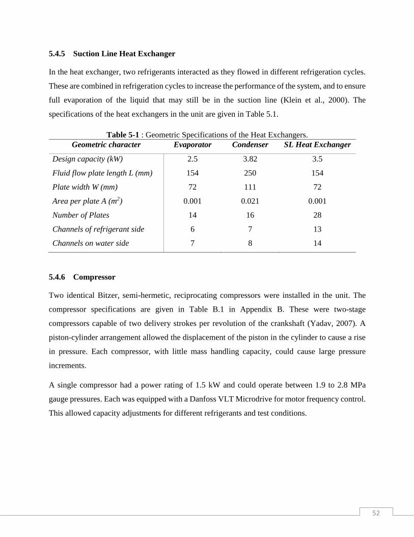
52
5.4.5 Suction Line Heat Exchanger
In the heat exchanger, two refrigerants interacted as they flowed in different refrigeration cycles.
These are combined in refrigeration cycles to increase the performance of the system, and to ensure
full evaporation of the liquid that may still be in the suction line (Klein et al., 2000). The
specifications of the heat exchangers in the unit are given in Table 5.1.
Table 5-1 : Geometric Specifications of the Heat Exchangers.
Geometric character Evaporator Condenser SL Heat Exchanger
Design capacity (kW) 2.5 3.82 3.5
Fluid flow plate length L (mm) 154 250 154
Plate width W (mm) 72 111 72
Area per plate A (m2) 0.001 0.021 0.001
Number of Plates 14 16 28
Channels of refrigerant side 6 7 13
Channels on water side 7 8 14
5.4.6 Compressor
Two identical Bitzer, semi-hermetic, reciprocating compressors were installed in the unit. The
compressor specifications are given in Table B.1 in Appendix B. These were two-stage
compressors capable of two delivery strokes per revolution of the crankshaft (Yadav, 2007). A
piston-cylinder arrangement allowed the displacement of the piston in the cylinder to cause a rise
in pressure. Each compressor, with little mass handling capacity, could cause large pressure
increments.
A single compressor had a power rating of 1.5 kW and could operate between 1.9 to 2.8 MPa
gauge pressures. Each was equipped with a Danfoss VLT Microdrive for motor frequency control.
This allowed capacity adjustments for different refrigerants and test conditions.

53
5.4.7 Suction Accumulator
A suction accumulator, also known as the surge drum, was positioned between the evaporator and
compressor. It consisted of a U-shaped pipe enclosed in a large cylindrical vessel. One end of this
pipe was connected to the suction line leading to the compressor, and the other end was open to
the vessel, as shown in Figure 5.4.
The pipeline from the evaporator was fixed to the top of the suction accumulator tank. Any liquid
refrigerant entering the tank was exposed to a large volume of this vessel, causing it to evaporate.
Consequently, only the gaseous refrigerant was permitted to pass through to the compressor.
Figure 5-4 : A Cross-sectional view of a Suction Accumulator (Extracted from Heldon, 2009a).
There were two tiny holes drilled into the U-shaped pipe, one was at the bottom where this pipe
bends and the other was at the top towards the exit to the compressor. The bottom hole was meant

54
to allow oil and some liquid refrigerant collected at the bottom of the tank to be channeled back to
the compressor. The apex hole was a pressure equalisation orifice. It was for equalising pressure
on both sides of the liquid in the pipe to prevent liquid refrigerant, which collected at the bottom
of the tank during the off-cycle, from being sucked into the compressor on start-up. Further
technical information on the suction accumulators can be found in Appendix B.
5.4.8 Moisture Indicator
As shown in Figure 5.1, moisture indicators were located immediately after the filter driers. There
were two moisture indicators in the unit used located in each section (MI-01 and MI-02). The ¼”
flare KSG2MF liquid line sight glass was utilised in the unit. The sight-glass had a dual purpose:
to confirm that sufficient refrigerant has been charged into the unit, and for indicating the presence
of moisture in the flowing refrigerant stream.
In assessing the amount of refrigerant in the system, the sight glass was positioned away from
valves and was fixed in a vertical position. In this position, the appearance of bubbles indicated
insufficient charge in the refrigeration system.
The colours on the sight glass were used to indicate the moisture content of the refrigerant flowing
in the refrigeration system. The signalling material was a porous filter paper saturated with a
chemical salt that is sensitive to moisture. As the refrigerant flowed past the indicator, a colour
change was observed relative to the moisture content of the refrigerant. A dark green colour
indicated that the refrigerant was dry and a yellow colour indicated a wet condition (presence of
moisture).
5.4.9 Filter Dryer
The SAD-163 solid core liquid line filter drier was selected for use in the test unit. It had small
spherical particles of high strength sintered desiccant in its core, combined with high-density filter
cloth which made an effective filter system. The drier was certified by the manufacturer to be
effective for use with different refrigerants such as R12, R134a, R410a, R404a, R22, R407C, R500

55
and R507. The pressure limit of the filter drier was specified as 4.7 MPa and insignificant pressure
loss was experienced when the liquid was flowing (Parker Hannifin Corporation, 2015).
The main purpose of the filter drier was to trap and eliminate moisture in the system, for
satisfactory operation and longevity of the equipment (Dennis et al., 2010). It could also act as a
physical filter for small particles suspendered in the refrigerant.
Possible sources of moisture in the refrigerant unit included the residue of wet lubricant,
refrigerant, and desiccant, leakage of water in the water-cooled heat exchanger, admission of
moisture-laden air via leaks, admission of moisture into the non-hermitic refrigerant system
through hoses and seals.
It was therefore essential to have a drier in the liquid line to remove the moisture/water present in
the refrigerant line. To enable a drier to collect and hold moisture it needed to contain a desiccant.
Substances usually used in the driers as dessicants are activated alumina, silica gel, and molecular
sieves. In this unit (shown in Figure 5.1), the filter dryer was positioned in the liquid line prior to
the expansion valve, to prevent moisture from freezing in the expansion valve.
5.4.10 Liquid Receivers
Liquid receivers labelled (LR-01 and LR-02) in Figure 5.1 were located downstream from the
condenser and heat exchanger respectively. These receivers maintained a constant liquid (only)
flow to the expansion valve and store excess refrigerant during operation at partial load. The valve,
installed at the outlet of the receiver, when shut, impeded refrigerant flow to the expansion valve.
By shutting this valve, the low-pressure side could be isolated and opened for service, and easily
restarted afterward. The bypass lines installed over the liquid receivers were used to gauge the
effect of the presence of the liquid receiver on the circulating flowrate and composition.
5.5 Instrumentation
5.5.1 Compact reconfigurable input and output (CRio)
The CRio is a data acquisition system that imports data from the pressure transducers and
temperature thermocouples situated at different points in the refrigerant unit and linked to a
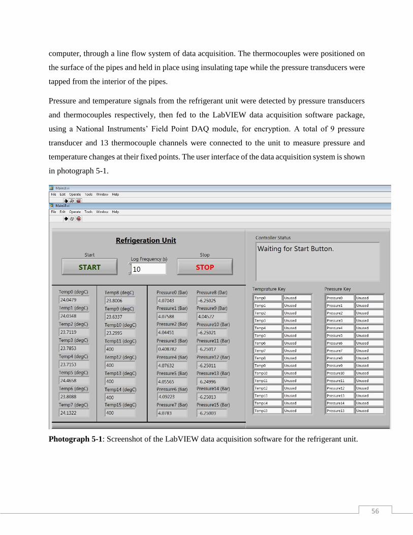
56
computer, through a line flow system of data acquisition. The thermocouples were positioned on
the surface of the pipes and held in place using insulating tape while the pressure transducers were
tapped from the interior of the pipes.
Pressure and temperature signals from the refrigerant unit were detected by pressure transducers
and thermocouples respectively, then fed to the LabVIEW data acquisition software package,
using a National Instruments’ Field Point DAQ module, for encryption. A total of 9 pressure
transducer and 13 thermocouple channels were connected to the unit to measure pressure and
temperature changes at their fixed points. The user interface of the data acquisition system is shown
in photograph 5-1.
Photograph 5-1: Screenshot of the LabVIEW data acquisition software for the refrigerant unit.

57
Specifics of the temperature probe and pressure transducers are given in Table 5.2. All channels
of data were sent to the computer for screen visualisation of the system operating parameters. This
data acquisition system allowed the user to access data from the unit as it operates.
Table 5-2 : Specifications of Instruments
Measured Variable Instrument Measurement
Range
Standard
Instrument
Uncertainty
Pressure Pressure Transducers 0-2.5 MPa ± 0.005 %
Temperature Thermocouples -20 to 100 ℃ ±0.03 oC
5.5.2 Variable Frequency Drive (VLT)
The variable frequency drive was used to adjust the speed of the compressor motor and to control
the capacity of the compressor. The VLT drive enables the user to vary the speed of the
compressor, thereby operating more efficiently at partial load. By closely matching the load,
variations in evaporating pressure and fluctuations in load temperature are minimised.
The VLT converts alternating current to direct current, and from this, it generates a simulated
alternating current signal at varying frequencies. The compressor was driven by the motor, which
operated at a speed proportional to the frequency input to the drive (Emerson Climate
Technologies AE4-1299 R9, 2010).
5.6 Water Circuits
The thermal load on the system received water that was electrically-heated in a hot water bath and
circulated through the evaporator. The heat transfer fluid (HTF) was selected due to its high heat
transfer coefficient, lower freezing point and the ease with which the bath maintained its
temperature in comparison to the air temperature of a room/container. Similarly, cold water
circulated through the condenser from an electrically-cooled water bath.
In both cases, elepon-seal-less 0.1 kW, centrifugal liquid pumps propelled the water circulation
from the water bath through PVC plastic pipes to the evaporator or condenser respectively and
back to the water bath. Both the evaporator and condenser bath temperatures were controlled by a
58
Grant TX150 digital temperature controller. Also, the water flow rate in both water baths was
measured by 1-10 L/min bottom/top entry water rotameter supplied by Ximatrix.
To maintain the low temperature of the cold sink, a PolyScience Flow through Chiller, Model KR-
80A was used. The return temperatures of liquid water to the water bath was measured by K-type
thermocouples inserted into the rubber hose. Calibrated rotameters controlled and measured water
flowrates through the heat exchangers.
To maintain a constant water temperature at the condenser inlet, two water baths were utilised, one
as a condenser water supply and the other as the hot water sink. The Polyscience temperature
Controllers (Model KR-80A) were used in the water baths.
5.7 Design Modifications carried out in this work.
On acquiring the unit and performing initial tests, some leaks were identified during pressure
testing. The major leaks were identified on the condensers outlet fittings and along the flexible
hose on the vibration eliminators. After the unit had been sealed, it was deemed necessary that
modifications were essential to ensure that the unit met the required operating standards.
The modified refrigeration unit used for the study is shown in Figure 5.5, with the red marking
indicating the changes made to the original design. These changes are described and explained in
the sections below:
5.7.1 Valves
The metering valve, SS-4MG-BU-MH, with a small orifice (ID= 0.00056 inch/1.42 mm) was
removed from the liquid line, as it could not facilitate the flow of refrigerant to the low-pressure
side. In its place, a stainless-steel Swagelok tube fitting Union Tee (ID=¼ inch/ 6.35 mm) was
installed with its branch-off end sealed by welding a piece of metal onto its orifice.

59
5.7.2 Evaporator water bath
A small (10 litres) water bath for the evaporator, was selected in the original design. It was replaced
with a larger (35 litres) water bath. This was motivated by the need to maintain the evaporator load
inlet temperature at 25 ℃. Using the 10-litre water bath, the chilled water from the evaporator
would reduce the temperature of the evaporator water bath. Thus water at a lower temperature than
the set value was pumped into the evaporator.
The continuous chilling of the heat transfer fluid, at the evaporator by the refrigerant, led to a
continuous decrease in the evaporator water bath temperature. Therefore, a larger bath (35litre)
replaced the smaller one (10litre) to enable the larger water volume to be maintained at an
unvarying temperature in the bath.
5.7.3 Evaporator Rotameter
Originally a rotameter measuring in the range of 1-10 litres per minute was selected to measure
the heat transfer fluid flowrate through the evaporator. However, at this flowrate the refrigeration
effect was not significant. This rotameter was replaced with a Swagelok plastic ball valve. This
was done to enable manual manipulation of the valve’s aperture to achieve lower flowrates, so that
a maximum refrigeration effect could be obtained at minimum evaporator load (Jerald and
Kumaran, 2014). The flow rate through the valve was determined using a calibrated orifice.
5.7.4 Condenser Chiller Bath
The 34 litres chiller bath in the original design proved inadequate to chill the warm water coming
from the condenser. The water had to be returned, at a lower set temperature, to cool the refrigerant
passing through the condenser. Thus a 50-litre water bath was placed alongside the smaller bath
(34-litre). The 50-litre bath was used as a cold sink, receiving warm water from the condenser
outlet to chill, before it flowed into the 34-litre bath. The smaller water bath was maintained at a
constant temperature to supply the condenser with water at a fixed temperature. This was done to
keep the heat sink at a constant temperature hence maintained a constant temperature in the system.
The baths were positioned in such a manner that the 50-litre bath was placed directly above the
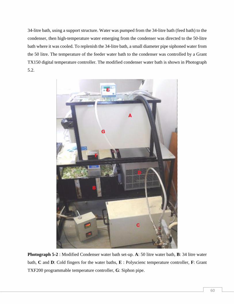
60
34-litre bath, using a support structure. Water was pumped from the 34-litre bath (feed bath) to the
condenser, then high-temperature water emerging from the condenser was directed to the 50-litre
bath where it was cooled. To replenish the 34-litre bath, a small diameter pipe siphoned water from
the 50 litre. The temperature of the feeder water bath to the condenser was controlled by a Grant
TX150 digital temperature controller. The modified condenser water bath is shown in Photograph
5.2.
Photograph 5-2 : Modified Condenser water bath set-up. A: 50 litre water bath, B: 34 litre water
bath, C and D: Cold fingers for the water baths, E : Polyscienc temperature controller, F: Grant
TXF200 programmable temperature controller, G: Siphon pipe.

61
5.7.5 Addition of Temperature Probes
Two Pt 100 temperature probes were added to the unit; one at the expansion valve outlet and the
other at the compressor outlet of the refrigerant line. This was motivated by the need to meter the
compressor discharge and the expansion valve exit temperature which was not catered for in the
original design. However, these could not be added to the LabVIEW data logging system as the
type of probes used were not compatible with the system’s hardware. Therefore, their readings
were manually recorded at regular intervals during system operation.
5.7.6 Charging Gauge
A 5.5/3.8 MPa VMG-2-R410A anti-collision series charging gauge was acquired to meter the
pressure difference between low and high pressure during the charging process. It was connected
to the suction and discharge valves on the compressor. It was used to monitor the pressure
variations in the suction and discharge line of the system during operation.
5.7.7 Insulation
The two heat exchangers were insulated to minimise the heat loss to the environment. The
evaporator was encapsulated with armflex rubber foam pipe insulation a low-temperature
insulating material, while the condenser was insulated with a high-temperature fiberglass
insulating material. A ½ inch/12.7 mm armflex rubber foam pipe insulating material was added to
the pipeline connecting the expansion valve exit and the evaporator inlet, the suction line and the
suction accumulator, to conserve energy in the system.
5.7.8 Mass Balance
A DE150K2DL Kern floor standing scale (non-automatic balance) was acquired to meter the mass
of the refrigerant charged into the unit. The scale had a maximum weight limit of 150 kg, a
minimum weight limit of 4 g, readability, and reproducibility of 5 g. Its uncertainty as specified
by the supplier was ± 2 g with a stabilisation time of 2.5 s. The measuring platform dimensions in

62
the format (B×D×M) mm were: (522×406×100) mm. The refrigerant tank was placed manually at
the centre of the weighing plate. When a stable weighing value was observed on the balance reader
the refrigerant tank weighing value could be read. Its operating temperature was between 5 and 35
oC, it could tolerate the air humidity of upto 80%. The following were observed in locating the
balance for use;
• was placed in a flat surface, away from open windows and doors to protect it against direct
droughts.
• was not be exposed direclty to sunlight to prevent temperature fluctuations and it was not
be exposed to extreme heat.
• was not to be exposed to extreme damp conditions for long periods of time.
Photographs 5-3 and 5-4 show the top view of the low pressure and the high-pressure sections of
the refrigerant test unit respectively.
Photograph 5-3: Top view of the low-pressure section of the refrigerant unit. HX-Inter-heat
exchanger, VLT-Variable frequency drive, CM-Compressor, LR-Liquid receiver, EV-
Evaporator, DR-Filter drier, TC-Temperature controller, WP-Water pipe, EV-WB-Evaporator
water bath, WCV-Evaporator water control valve.

63
Photograph 5-4: Top view of the high-pressure section of the refrigerant test unit. CH-Charging
point, CM-Compressor, CN-Condenser, CRio-Data acquisition unit, DR-Filter drier, EV-
Evaporator, EX-Expansion valve, LP-Liquid pump, LR-Liquid receiver, MI-Moisture indicator,
OS-Oil separator, SG-Sight glass, VLT-Variable frequency drive, CG-Charging Gauge, WP-
Water pipe, CWB- Condenser water bath.

64
VLT
1
VLT
2COMPRESSOR 2
CONTROLPANEL
COMPRESSOR 1CONTROL
PANEL
CN-01
HX-01
EV-01
V-5
V-10
V-1
V-4
EX-02
EX-01
SG-01
CP-01
CP-03
T2
T1
T6
SA-01 SA-02
OS-02
V-6
V-2
V-12
MI-01
LR-01
MI-02
LR-02
MV-2
V-3
V-8
CH-02
CH-03
CH-04
CH-01
CP-02
V-11
V-13V-9
CV-03
CV-04
CV-01
P0
P2
P6
T0P4
CV-02
T10 P3
T4 P9
T7 P1
P5
DR-01
V-7
DR-02
T8 P7
WATER
BATH 2
EV WATER
BATHT3
OS-01
T9
CM-02CM-01
T5
CRio
LP-02
RT-01
T11
T12
WATER
BATH 1LP-01
Figure 5-5 : Schematic Design of Modified test unit
CH-Charging point, CM-Compressor, CN-Condenser, CP-Connection point, CRio-Data acquisition unit, CV-Charging valve, DR-Filter drier, EV-
Evaporator, EX-Expansion valve, HX-Inter-heat exchanger, LP-Liquid pump, LR-Liquid receiver, MI-Moisture indicator, OS-Oil separator, P-
Pressure transducer, RT-Rotameter, SA-Suction accumulator, SG-Sight glass, T-Thermocouple, V-Valve, VLT-Variable frequency drive.

65
Chapter 6
6 Experimental Procedure
This chapter outlines the equipment preparation procedure prior to use as well as the operation
procedure for carrying out experimental measurements. Special emphasis is on the simple
vapour compression cycle which is the focus of this study.
6.1 Preparation
It important to ensure that there are no leaks in the system; this is checked by carrying out the
leak testing procedure. This system is purged of air and moisture by filling it with nitrogen gas.
This is then vented and the system is evacuated using a vacuum pump. The desired operating
cycle is achieved by correct configuration of system lines via the use of flexible hoses and
manipulation of valves.
6.2 Leak Testing and Detection
It is imperative to ensure that there are no leaks in the system, prior to its use as the leaks would
not only affect the performance and control aspects of operation but may also pose a health
hazard. The different leak detection procedures for vacant and charged systems are described
below. Since all pathways and fittings could not be tested simultaneously the following
procedure should be repeated when necessary for the different cycle configurations so that no
possible leaks are overlooked. The leak testing procedure is outlined below:
i. Leak testing is effective on a vacant system.
ii. Set the valves such that the whole unit can be pressurised at once through a single
charging point.
iii. Use oxygen-free nitrogen (OFN) to pressurise the system via any of the four charging
points. Do not use oxygen or other industrial gases. When using dry air isolate the
compressor (i.e. keep shut-off valves closed) to avoid compressor oil oxidation.
iv. Test pressure should not exceed the maximum operating pressure indicated on the
compressor nameplate (i.e. 1.9 MPa low-pressure limit).
v. Pressurize the unit to a constant pressure value in all sections and shut off the charging
port.

66
vi. Isolate different components and monitor the pressure readings from various
transducers overnight or over an extended period. Pressure drop is indicative of a leak/s
in that section.
vii. To pinpoint the source of the leak, apply a soapy solution or SNOOP® to joints and
other places susceptible to leaks. Formation of bubbles in an area where the soapy
solution is applied is an indication of a leak.
viii. Alternatively, an electronic leak detector can be used. With this method, Helium gas
must be used to get the desired outcome.
6.3 Start-Up
6.3.1 Vacant System
i. Wear goggles and gloves.
ii. Check the oil level in the compressor: It should be between ½ and ¾ full in the
compressor sight glass.
iii. Connect hoses for the desired cycle and set the valve to direct flow in desired directions.
iv. Evacuate the system to a vacuum level of between 53.2 - 26.6 kPa abs, then isolate the
vacuum pump. N.B.: Do not evacuate to below 26.6 kPa abs as it will degas particles
of the refrigerant oil.
v. Set the heat transfer fluid bath temperatures and leave them to stabilise.
vi. Circulate respective HTFs through the evaporator and the condenser at desired flow
rates.
vii. Charge the charging cell with slightly larger volume of refrigerant than is necessary to
cater for any unforeseen hiccups.
viii. Connect the charging hosepipe from the valve at the bottom of charging cylinder to the
valve on the refrigerant cylinder. The refrigerant cylinder is kept upright so that only
gas leaves the refrigeration tank. When the liquid refrigerant is required the tank must
be inverted so that the valve is down, with this arrangement, only liquid refrigerant will
flow out of the tank.
ix. Connect the charging hose to charging point CH-01 which is at the evaporator inlet
when charging a liquid refrigerant or to CH-02 at the suction line when charging vapour
refrigerant.
x. To quantify the amount of refrigerant charged into the unit the charging cylinder should
be weighed on a digital balance.
67
xi. The refrigerant is admitted into the system until the pressure of the cylinder is reached,
that is, the pressure of the unit is equal to that of the charging cylinder.
xii. At this point operate the refrigerant unit by turning on the compressor (Coggins, 2007).
xiii. With the compressor running continue charging the unit, adjusting the expansion valve
in the processing unit until a superheat of between 5-12 0C and a sub-cooling in the
range of 5-15 0C is achieved.
xiv. The sight glass can also be used to gauge when enough refrigerant has been loaded into
the cell; this is shown by the absence of bubbles in the glass.
xv. The system is given about 30 - 40 minutes to reach steady state before results are logged
at one-minute intervals for a minimum period of 30 minutes.
xvi. N.B.: Compressor should not be started more than eight times per hour, so as to protect
the start capacitors and avoid compressor overheating due to locked up rotor current.
xvii. N.B.: Charging Vapour Refrigerant: CH-02 situated at the inlet to the second
compressor and CH-03 at the inlet to the first compressor are used for the admission of
pure fluid, vapour refrigerants. Following the necessary connections, the refrigerant is
then admitted into the system until it has reached the cylinder pressure. The compressor
is then started, and the expansion valve reduces pressure in the charging line to a level
below that of the cylinder so that the refrigerant will continue to flow into the system.
Alternatively, the charging cell pressure may be gradually raised in the hot bath at less
than 40 0C (Hundy et al., 2008) such that the required charge may be admitted before
switching the compressor on without the use of the expansion valve. This method of
charging is less time-consuming.
Charging Liquid Refrigerant: CH-04 upstream from the inter-heat exchanger and
CH-01 at the inlet to the evaporator are used for the admission of (pre-mixed) liquid
refrigerant blends. For new mixtures, charge a lower vapour pressure refrigerant at the
compressor inlet first, followed by a higher vapour pressure fluid (Jung et al., 2000).
6.3.2 Charged System
i. Set the HTF bath temperatures and leave to stabilize.
ii. Ensure that all valves are configured to the desired cycle.
iii. Circulate the HTFs, at the desired flowrate, through the condenser and evaporator.
iv. Start the compressor.
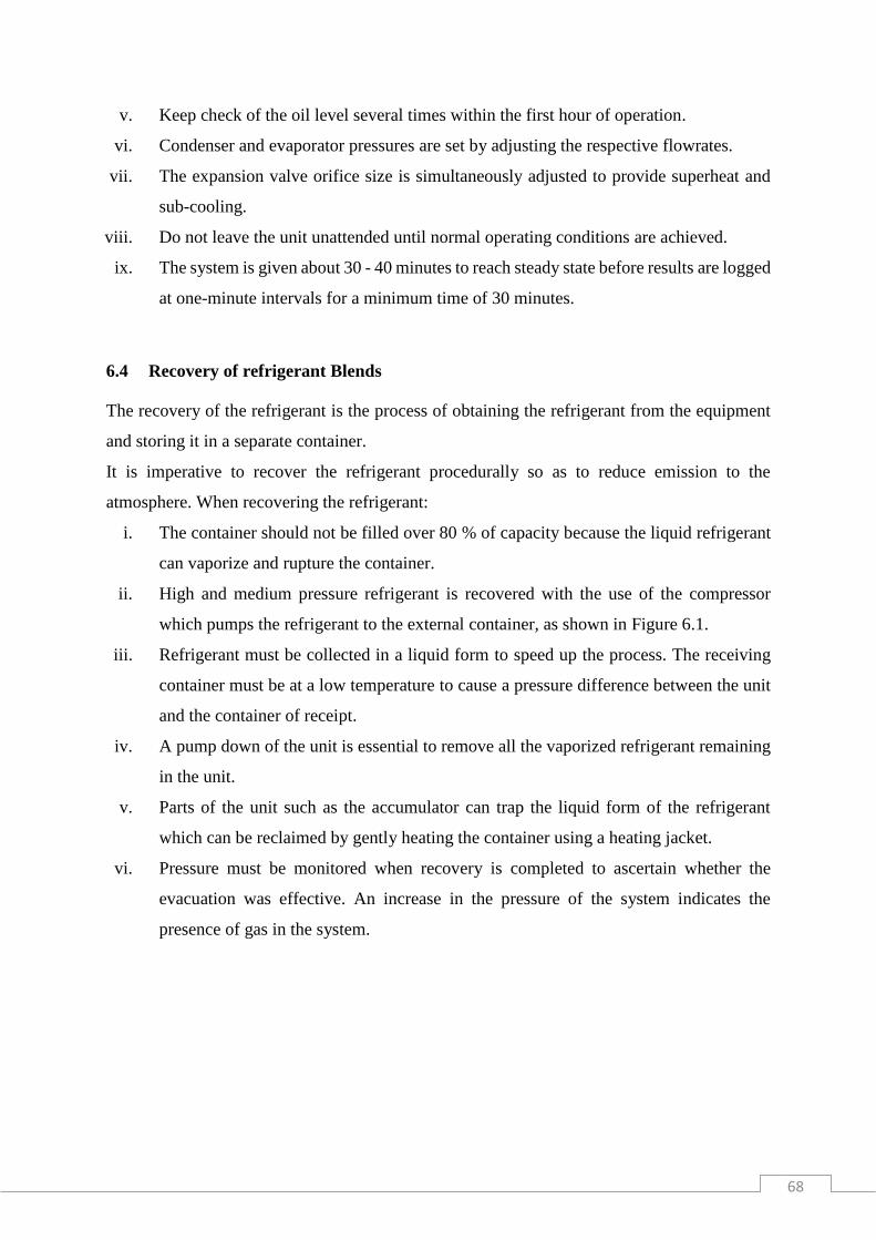
68
v. Keep check of the oil level several times within the first hour of operation.
vi. Condenser and evaporator pressures are set by adjusting the respective flowrates.
vii. The expansion valve orifice size is simultaneously adjusted to provide superheat and
sub-cooling.
viii. Do not leave the unit unattended until normal operating conditions are achieved.
ix. The system is given about 30 - 40 minutes to reach steady state before results are logged
at one-minute intervals for a minimum time of 30 minutes.
6.4 Recovery of refrigerant Blends
The recovery of the refrigerant is the process of obtaining the refrigerant from the equipment
and storing it in a separate container.
It is imperative to recover the refrigerant procedurally so as to reduce emission to the
atmosphere. When recovering the refrigerant:
i. The container should not be filled over 80 % of capacity because the liquid refrigerant
can vaporize and rupture the container.
ii. High and medium pressure refrigerant is recovered with the use of the compressor
which pumps the refrigerant to the external container, as shown in Figure 6.1.
iii. Refrigerant must be collected in a liquid form to speed up the process. The receiving
container must be at a low temperature to cause a pressure difference between the unit
and the container of receipt.
iv. A pump down of the unit is essential to remove all the vaporized refrigerant remaining
in the unit.
v. Parts of the unit such as the accumulator can trap the liquid form of the refrigerant
which can be reclaimed by gently heating the container using a heating jacket.
vi. Pressure must be monitored when recovery is completed to ascertain whether the
evacuation was effective. An increase in the pressure of the system indicates the
presence of gas in the system.
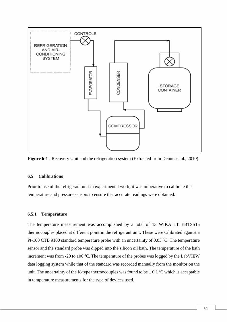
69
Figure 6-1 : Recovery Unit and the refrigeration system (Extracted from Dennis et al., 2010).
6.5 Calibrations
Prior to use of the refrigerant unit in experimental work, it was imperative to calibrate the
temperature and pressure sensors to ensure that accurate readings were obtained.
6.5.1 Temperature
The temperature measurement was accomplished by a total of 13 WIKA T1TEBTSS15
thermocouples placed at different point in the refrigerant unit. These were calibrated against a
Pt-100 CTB 9100 standard temperature probe with an uncertainty of 0.03 oC. The temperature
sensor and the standard probe was dipped into the silicon oil bath. The temperature of the bath
increment was from -20 to 100 oC. The temperature of the probes was logged by the LabVIEW
data logging system while that of the standard was recorded manually from the monitor on the
unit. The uncertainty of the K-type thermocouples was found to be ± 0.1 oC which is acceptable
in temperature measurements for the type of devices used.

70
6.5.2 Pressure
Nine WIKA A-10 pressure transducers (0-25 MPa rating) were used for pressure measurements
in the refrigerant unit. The pressure transducers were calibrated against a standard CPT 600
pressure transducer with an operating range of 0-25 MPa, with an accuracy of 0.005% of the
full scale, calibrated by WIKA South Africa. The data collected in the calibration process was
fitted into a first order polynomial, and the accuracy of each transducer was ± 0.026 MPa.
6.5.3 Flowrate
A liquid ½” bottom/top entry brass rotameter was used to meter the water flow rate through
the condenser. Water was pumped through the rotameter, which had a needle valve at the
bottom inlet to control the amount of incoming fluid. The rotameter was graduated to meter
flow in the range of 0.5-10 L/min, with an increment of 0.5 L, while a float was used to set the
flowrate at to the desired value.
In the calibration of the rotameter, water was pumped into a measuring cylinder for a minute;
the flow rate was then increased. The process was timed using a stopwatch, and repeated runs
were performed with the average value being used. The data obtained was then fitted to a first
order polynomial. A ball valve controlled the water flow through the evaporator. The flow rate
was determined by repeatedly timing water flow into a 5000-ml measuring cylinder. By
changing the orifice opening, markings were made on the orifice, with each marking denoting
a specific flowrate.
6.5.4 Experimental Uncertainty Measurements
In computing the uncertainty in the temperature and pressure measurements in this study a full
description of formulaes and methods used are given in Appendix E. The combined
uncertainty 𝑢𝑐(𝑥) is calculated from the uncertainty which arises from any of the two
categories of uncertainty type A or type B. The type A uncertainty is evaluated by statistical
methods in which the mean is taken to represent the true value (Taylor and Kuyatt, 1994). It is
calculated by the flowing formula:

71
𝑢𝑖(𝑥) =𝜎
√𝑁 6.1
where 𝜎 the standard deviation of the data and N is the number of data points. Type B
uncertainty is evaluated by several methods and information related to the measurements. The
uncertainty can lie anywhere between the distribution and such distributions are known as
rectangular. They are represented by:
𝑢𝑖(𝑥) =𝑏
√36.2
where b is the half the width of the interval. The rectangular distribution model is always the
default model in the absence of any other information (Taylor and Kuyatt, 1994).The combined
uncertainty of temperature is given by:
𝑢𝑐(𝑇) = ±√𝑢𝑐𝑎𝑙𝑖𝑏(𝑇)2 + 𝑢𝑟𝑒𝑝(𝑇)2 + 𝑢𝑖𝑛𝑠𝑡𝑟(𝑇)2
6.3
where 𝑢𝑟𝑒𝑝(𝑇) denotes the standard uncertainty because of repeatability of a
measurement, 𝑢𝑖𝑛𝑠𝑡𝑟(𝑇) is the uncertainty of the Pt-100 standard temperature probe and
𝑢𝑐𝑎𝑙𝑖𝑏(𝑇) denotes the standard uncertainty as a result of temperature calibration and is
determined by:
𝑢𝑐𝑎𝑙𝑖𝑏(𝑇) = ±√𝑢𝑠𝑡𝑑(𝑇)2 + 𝑢𝑐𝑜𝑟𝑟(𝑇)2
6.4
where 𝑢𝑐𝑜𝑟𝑟(𝑇) denotes the standard uncertainty because of the temperature calibration
correlation and 𝑢𝑠𝑡𝑑(𝑇) denotes the standard uncertainty inherent in the standard temperature
probe. The value used for the calibration uncertainty in this study (in Table 7.5) was the largest

72
value obtained in the calibration of all the seven temperature sensors. Likewise, the combined
standard uncertainty in pressure is calculated by:
𝑢𝑐(𝑃) = ±√𝑢𝑐𝑜𝑟𝑟(𝑃)2 + 𝑢𝑟𝑒𝑝(𝑃)2 + 𝑢𝑠𝑡𝑑(𝑃)2 + 𝑢𝑎𝑡𝑚(𝑃)2
6.5
where 𝑢𝑐𝑜𝑟𝑟(𝑃) is the standard uncertainty due to the pressure calibration correlation (Type B),
𝑢𝑠𝑡𝑑(𝑃) is the standard uncertainty of the pressure transducer, and 𝑢𝑟𝑒𝑝(𝑃) is the standard
uncertainty due to the repeatability of the pressure measurement. Likewise, the value used in
the study for the calibration uncertainty in pressure was the largest values of all the values
obtained from four pressure transmitters.
Rotameters measure the water flowrates through the condenser and evaporator. The combined
uncertainty of flowrate is given by:
𝑢𝑐(𝐹) = ±√𝑢𝑐𝑜𝑟𝑟(𝐹)2+𝑢𝑟𝑒𝑝(𝐹)2
6.4
where 𝑢𝑟𝑒𝑝(𝐹) is the standard uncertainty due to the repeatability of the flowrate measurement
and 𝑢𝑐𝑜𝑟𝑟(𝑃) is the standard uncertainty due to flowrate calibration correlation.

73
Chapter 7
7 Results and Discussions
The results obtained in the experiments and simulations carried out in this study are presented,
analysed and discussed in this chapter. This chapter consists of three main sections. In the first
section results obtained in the commissioning stage are presented and analysed, the second
section is a comparative study of the performance of the three refrigerants studied. The third
section is a comparison of the experimental performance of the refrigerants with the theoretical
performance obtained from Aspen Plus ® simulations. In the final section, the refrigerant blends
investigated are discussed with the aid of the simulated results. Firstly, the chemical purity,
physical properties of refrigerants and uncertainty in measurements are discussed.
7.1 Chemical Purity and Physical Properties of Refrigerants
The chemical purity and supplier details are presented in Table 7.1.
Table 7-1 : Details of the chemicals used in this study.
Refrigerant CAS Number Supplier Purity (*wt %)
R134a
(1,1,1,2-Tetrafluoroethane)
811-97-2 Afrox > 99.7
R507a
(Pentafluoroethane/1,1,1-
Trifluoroethane (50/50))
354-33-6/420-46-2 Afrox > 99.7
R125
(Pentafluoroethane)
354-33-6 Kovco > 99.5
R413a
(Octafluoropropane/1,1,1,2-
Tetrafluoroethane/Isobutane
(9/88/3))
811-97-2/76-19-7/ 75-
28-5
Kovco > 99.7
*Purity stated by the supplier.
The chemicals were of high purity as per supplier specifications. It is imperative to use
chemicals of high purity in refrigeration operations to avoid the clogging of the expansion valve
orifice and the contamination of the compressor oil. Water used in the water baths, was
acquired from the municipality water supply line.
Table 7.2 presents the physical properties of the refrigerants used in this study. As discussed
by Venkatarathnam and Murthy (2012), the critical temperature and normal boiling point are
fundamental thermodynamic properties of a refrigerant which influence the vapour pressure

74
and the latent heat of vaporisation. The refrigerants selected in this study have comparable
critical pressures and temperatures, boiling points and molecular weights. Furthermore, their
selection was influenced by their availability and zero ODP rating. However, while their GWP
is in an acceptable range, the new European Union Fluorinated greenhouse gases (EU F-Gas)
regulation states that from 2020, refrigerants with GWP value less than 2500 will be acceptable
in refrigeration applications (Bitzter, 2014).
Table 7-2 : Thermodynamic Properties of Refrigerants
Refrigerant R134aa R125b R507ac R413ad
Molecular weight (g mol-1) 102 120 98.86 103.96
Critical Temperature (℃) 101.1 66.2 70.9 101.3
Critical Pressure (MPa) 4.06 3.63 3.79 4.11
Bubble point (℃) -26.1 -54.6 -46.7 -35
Dew point (℃) -101 - - -28.1
Temperature Glide (℃) 0 0 0 0
ODP 0 0 0 0
GWP 1300 3400 3900 1900 a (Karagoz et al., 2004) , b (Mohanraj et al., 2011) , c (Arora and Kaushik, 2008), d (ISCEON
Refrigerants, 1998). (–) not determined.
7.2 Uncertainty in Measurements
In experimental work, it is imperative to maintain high accuracy and precision to ensure
credibility of the results obtained. To ensure this, clinical adherence to the experimental
procedure, careful equipment handling, and calibration of the sensors is crucial. The calibration
is done to ensure that the measuring device is reporting a true measurand.
The result of a measurement is an estimate of the value of the specific quantity subject to a
measurement called the measurand. Consequently, for the result to be complete, a numerical
value of its uncertainty is supposed to be accompanying it.
In computing the uncertainty of a measurement, the instrumental error, calibration uncertainty,
and repeatability uncertainty were incorporated. Appendix D gives the methods and formulas
for calculating the uncertainty of temperature, pressure and flow rate measurements. The
calibration procedures followed were discussed in Section 6.5 of this study. Tables 7.3 and 7.4
present the calibration information for the temperature sensors and pressure transducers
respectively. The trend line equations in Table 7.3 were generated using an Excel worksheet
by plotting the standard temperature obtained from the WIKA standard probe against the
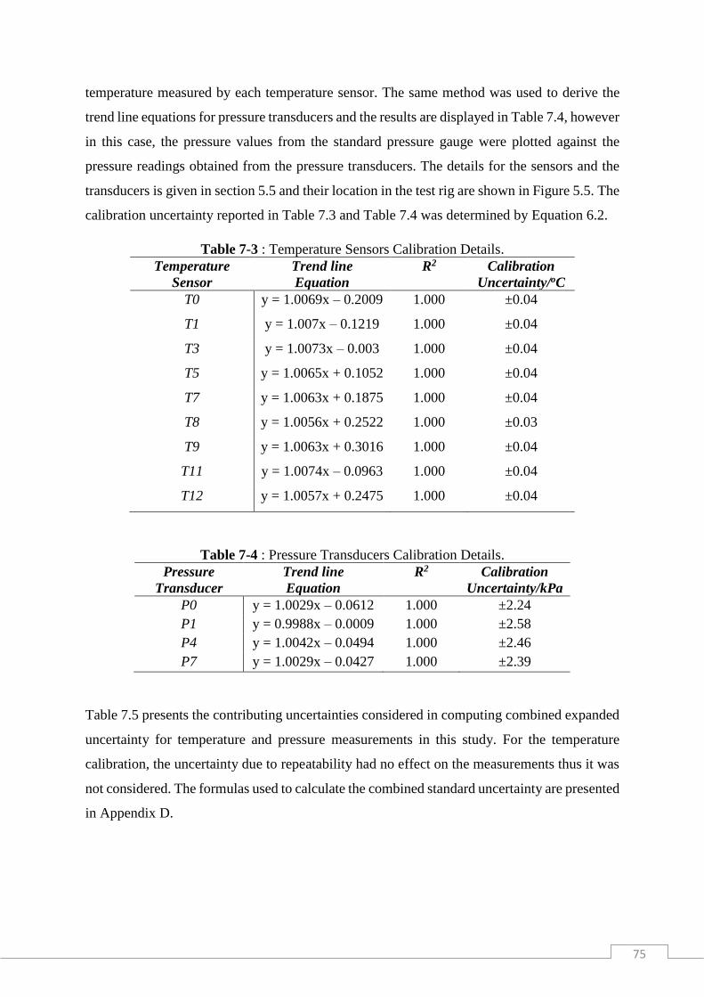
75
temperature measured by each temperature sensor. The same method was used to derive the
trend line equations for pressure transducers and the results are displayed in Table 7.4, however
in this case, the pressure values from the standard pressure gauge were plotted against the
pressure readings obtained from the pressure transducers. The details for the sensors and the
transducers is given in section 5.5 and their location in the test rig are shown in Figure 5.5. The
calibration uncertainty reported in Table 7.3 and Table 7.4 was determined by Equation 6.2.
Table 7-3 : Temperature Sensors Calibration Details.
Temperature
Sensor
Trend line
Equation
R2 Calibration
Uncertainty/oC
T0
T1
y = 1.0069x – 0.2009
y = 1.007x – 0.1219
1.000
1.000
±0.04
±0.04
T3 y = 1.0073x – 0.003 1.000 ±0.04
T5 y = 1.0065x + 0.1052 1.000 ±0.04
T7 y = 1.0063x + 0.1875 1.000 ±0.04
T8 y = 1.0056x + 0.2522 1.000 ±0.03
T9 y = 1.0063x + 0.3016 1.000 ±0.04
T11 y = 1.0074x – 0.0963 1.000 ±0.04
T12 y = 1.0057x + 0.2475 1.000 ±0.04
Table 7-4 : Pressure Transducers Calibration Details.
Pressure
Transducer
Trend line
Equation
R2 Calibration
Uncertainty/kPa
P0 y = 1.0029x – 0.0612 1.000 ±2.24
P1 y = 0.9988x – 0.0009 1.000 ±2.58
P4 y = 1.0042x – 0.0494 1.000 ±2.46
P7 y = 1.0029x – 0.0427 1.000 ±2.39
Table 7.5 presents the contributing uncertainties considered in computing combined expanded
uncertainty for temperature and pressure measurements in this study. For the temperature
calibration, the uncertainty due to repeatability had no effect on the measurements thus it was
not considered. The formulas used to calculate the combined standard uncertainty are presented
in Appendix D.
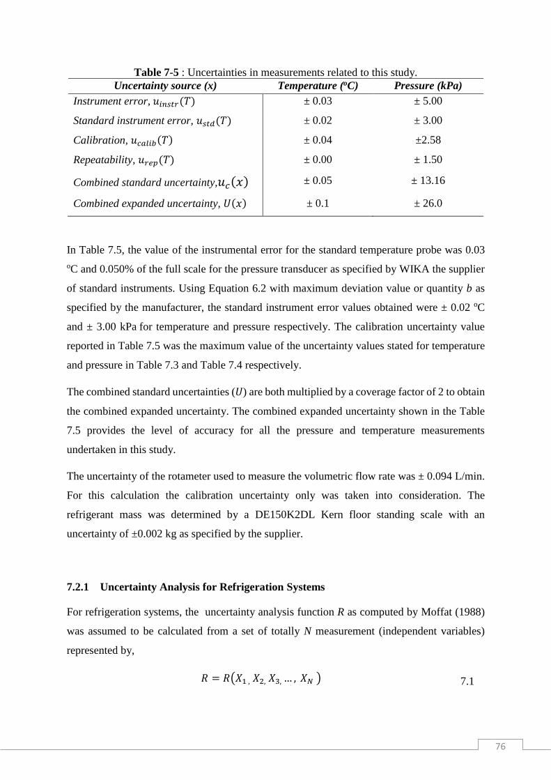
76
Table 7-5 : Uncertainties in measurements related to this study.
Uncertainty source (x) Temperature (oC) Pressure (kPa)
Instrument error, 𝑢𝑖𝑛𝑠𝑡𝑟(𝑇) ± 0.03 ± 5.00
Standard instrument error, 𝑢𝑠𝑡𝑑(𝑇) ± 0.02 ± 3.00
Calibration, 𝑢𝑐𝑎𝑙𝑖𝑏(𝑇) ± 0.04 ±2.58
Repeatability, 𝑢𝑟𝑒𝑝(𝑇) ± 0.00 ± 1.50
Combined standard uncertainty,𝑢𝑐(𝑥) ± 0.05 ± 13.16
Combined expanded uncertainty, 𝑈(𝑥) ± 0.1 ± 26.0
In Table 7.5, the value of the instrumental error for the standard temperature probe was 0.03
oC and 0.050% of the full scale for the pressure transducer as specified by WIKA the supplier
of standard instruments. Using Equation 6.2 with maximum deviation value or quantity b as
specified by the manufacturer, the standard instrument error values obtained were ± 0.02 oC
and ± 3.00 kPa for temperature and pressure respectively. The calibration uncertainty value
reported in Table 7.5 was the maximum value of the uncertainty values stated for temperature
and pressure in Table 7.3 and Table 7.4 respectively.
The combined standard uncertainties (𝑈) are both multiplied by a coverage factor of 2 to obtain
the combined expanded uncertainty. The combined expanded uncertainty shown in the Table
7.5 provides the level of accuracy for all the pressure and temperature measurements
undertaken in this study.
The uncertainty of the rotameter used to measure the volumetric flow rate was ± 0.094 L/min.
For this calculation the calibration uncertainty only was taken into consideration. The
refrigerant mass was determined by a DE150K2DL Kern floor standing scale with an
uncertainty of ±0.002 kg as specified by the supplier.
7.2.1 Uncertainty Analysis for Refrigeration Systems
For refrigeration systems, the uncertainty analysis function R as computed by Moffat (1988)
was assumed to be calculated from a set of totally N measurement (independent variables)
represented by,
𝑅 = 𝑅(𝑋1 , 𝑋2, 𝑋3, … , 𝑋𝑁 ) 7.1

77
Therefore the uncertainty of the result R can be computed by summing up the uncertainties of
singular terms using a root-sum-square method (Hoşöz, 2005), i.e.
𝛿𝑅 = {∑ (𝜕𝑅
𝜕𝑋𝑖𝜕𝑥𝑖)
2𝑁
𝑖=1
}
12⁄
7.2
The uncertainty of the following parameters 𝑄𝑒𝑣𝑎𝑝, ��𝑐𝑜𝑚𝑝 and COP can be determined by
Equation 7.2. Hoşöz (2005) using Moffat’s method in the study to investigate the performance
of refrigerant R134 in a single-stage and cascade refrigeration systems. The uncertainty values
of 𝑄𝑒𝑣𝑎𝑝, ��𝑐𝑜𝑚𝑝 and COP obtained were 4.4%, 16.5%, and 16.8% respectively. Likewise,
Datta et al. (2014) employed Moffat’s methods of computing uncertainties in the study of the
performance of automotive air conditioning system. The uncertainties of 𝑄𝑒𝑣𝑎𝑝, ��𝑐𝑜𝑚𝑝 and
COP were reported to be 1.75%, 1.76% and 4.72% respectively at the highest charge level.
7.3 Commissioning of unit using R134a
Refrigerant R134a was selected for use in the commissioning stage due to its widespread usage
in refrigeration systems and the availability of vast amount of data published on it. Mollier
charts were used to analyse the experimental data to obtain the derived results such as COP,
compressor work, cooling effect and compressor efficiency.
Test runs were undertaken to confirm that the unit was fit for use on a simple VC cycle. To
accomplish this objective, three test runs were carried out at set conditions to assess the
functionality of the unit and to produce repeatable and consistent readings within experimental
uncertainty. In achieving this, the critical operating parameters were kept constant. These
parameters were as follows: mass of the refrigerant, compressor power setting, expansion valve
setting, evaporator water flow rate, condenser cooling water temperature, and condenser water
flow rate.
The operating parameters selected to conduct the experiments were a refrigerant mass (charge)
of 3.115 kg, condenser water flow rate of 2.75 L/min and a bath temperature of 20 ℃. The
evaporator flow rate was 0.58 L/min and a bath temperature of 25 ℃ and the 0.128-inch/3.25

78
mm orifice Swagelok expansion valve was set in the half open position to achieve the desired
level of superheating at the evaporator outlet. The compressor was set to 2.20 kW, the voltage
to 400 V, current to 3 Amps and an operational speed of 1420 rpm.
Whilst conducting the experiments, the room temperature was maintained at approximately 22
oC at all times, with the aid of an air-conditioning unit. This temperature control was
implemented to eliminate the effects of external temperature variations to ensure a fair test
environment. However, ambient temperature fluctuations were experienced during the
experiments due to the malfunctioning of the air-conditioning system. The system was assumed
to have reached steady-state when temperature and pressure fluctuations had ceased at the
condenser and evaporator refrigerant entry and exit points. The system took approximately 40
minutes to stabilise. Once the system had stabilised, the temperature and pressure readings
were logged every minute, for more than 30 minutes on the LabVIEW data logging system
connected to the computer. The experimental period was limited by the temperature increase
in the condenser water bath, i.e., the heat sink.
The reproducibility of the measured results as illustrated in Table 7.6. These results validated
the functionality of the unit as the pressure was maintained at a fixed value for each cycle run,
indicating no pressure loss or loss of refrigerant to other compartments of the unit or the
environment.
Table 7-6 : Results during commissioning of unit using R134a.
Variable Run 1 Run 2 Run 3 Run 4
Evaporator Refrigerant Inlet temp (℃) -3.2 -3.0 -2.4 -3.4
Evaporator Refrigerant Outlet temp (℃) -2.3 -1.3 -1.3 -2.5
Compressor Refrigerant Inlet temp (℃) 5.3 6.7 7.1 4.6
Condenser Refrigerant Inlet temp (℃) 56.8 52.9 55.7 54.6
Condenser Refrigerant Outlet temp (℃) 24.7 24.2 24.6 24.2
Evaporator Inlet press (kPa) 233 234 238 228
Evaporator Outlet press (kPa) 226 226 231 220
Condenser inlet press (kPa) 692 673 679 674
Condenser Outlet press (kPa) 687 668 674 669
The variance in the temperature readings presented in Table 7.6 is acceptable relative to the
experimental uncertainty with the largest temperature difference between runs being 3.9 ℃
obtained from condenser refrigerant inlet temperatures from run 1 and run 2. Likewise, the
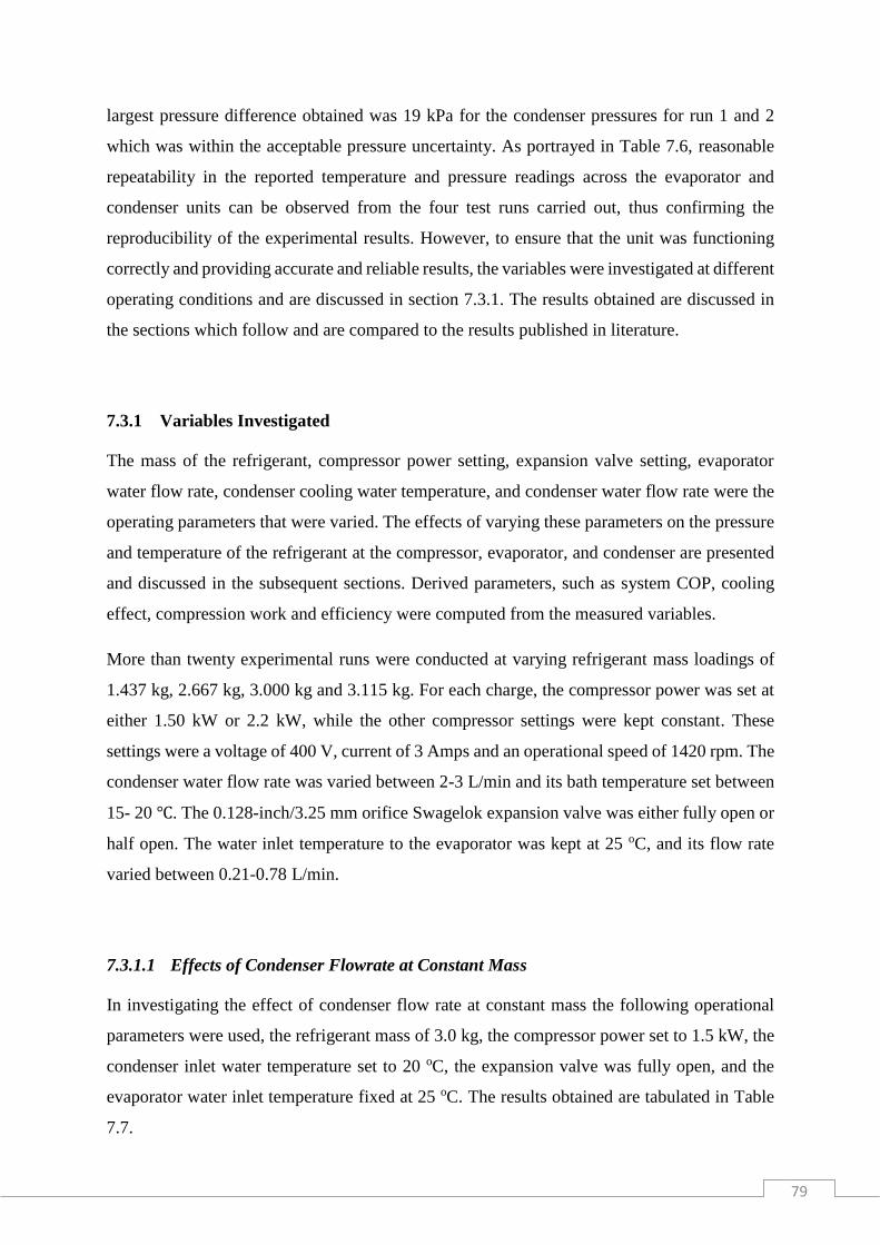
79
largest pressure difference obtained was 19 kPa for the condenser pressures for run 1 and 2
which was within the acceptable pressure uncertainty. As portrayed in Table 7.6, reasonable
repeatability in the reported temperature and pressure readings across the evaporator and
condenser units can be observed from the four test runs carried out, thus confirming the
reproducibility of the experimental results. However, to ensure that the unit was functioning
correctly and providing accurate and reliable results, the variables were investigated at different
operating conditions and are discussed in section 7.3.1. The results obtained are discussed in
the sections which follow and are compared to the results published in literature.
7.3.1 Variables Investigated
The mass of the refrigerant, compressor power setting, expansion valve setting, evaporator
water flow rate, condenser cooling water temperature, and condenser water flow rate were the
operating parameters that were varied. The effects of varying these parameters on the pressure
and temperature of the refrigerant at the compressor, evaporator, and condenser are presented
and discussed in the subsequent sections. Derived parameters, such as system COP, cooling
effect, compression work and efficiency were computed from the measured variables.
More than twenty experimental runs were conducted at varying refrigerant mass loadings of
1.437 kg, 2.667 kg, 3.000 kg and 3.115 kg. For each charge, the compressor power was set at
either 1.50 kW or 2.2 kW, while the other compressor settings were kept constant. These
settings were a voltage of 400 V, current of 3 Amps and an operational speed of 1420 rpm. The
condenser water flow rate was varied between 2-3 L/min and its bath temperature set between
15- 20 ℃. The 0.128-inch/3.25 mm orifice Swagelok expansion valve was either fully open or
half open. The water inlet temperature to the evaporator was kept at 25 oC, and its flow rate
varied between 0.21-0.78 L/min.
7.3.1.1 Effects of Condenser Flowrate at Constant Mass
In investigating the effect of condenser flow rate at constant mass the following operational
parameters were used, the refrigerant mass of 3.0 kg, the compressor power set to 1.5 kW, the
condenser inlet water temperature set to 20 oC, the expansion valve was fully open, and the
evaporator water inlet temperature fixed at 25 oC. The results obtained are tabulated in Table
7.7.

80
Table 7-7 : Effects of the Condenser Flowrate on system.
Variable Run 1 Run 2 Run 3
Condenser Water flowrate (L/min) 2.0 2.5 3.0
Evaporator Refrigerant Inlet Temp (oC) -2.7 -2.5 -1.7
Evaporator refrigerant Outlet Temp (oC) 12.9 11.4 -1.5
Compressor inlet Temp (oC) 14.1 11.8 5.2
Cooling Effect (kJ/kg) 178 177 164
Expansion Valve Orifice/Inch 0.128a 0.128a 0.128a
COP 4.68 5.36 3.64
% Compressor Efficiency 73.7 71.1 55.6
Compression Ratio 3.30 3.17 3.11 a Fully open position
When the condenser flow rate was increased it can be observed from Table 7.7 that the
evaporator inlet temperature of the refrigerant increased as well, whereas, the evaporator outlet
temperature, compression ratio, and compressor efficiency decreased. The decrease in the
cooling effect as the condenser flow rate increased was as a result of the reduction in the level
of superheating at the evaporator outlet (as observed from the evaporator outlet temperature
readings of 12.9, 11.4, and -1.5 ℃ in each of the runs). From the results obtained, the refrigerant
exhibited the best performance at a condenser flowrate of 2.5 L/min, with the highest COP of
5.36. The level of superheating at the evaporator outlet is more evident in run 3 than in runs 1
and 2. This was due to the gradual increase of the condenser flow rate by 0.5 L/m from run 1
to run 3. Thus, the heat sink in run 3 had sufficient capacity to cool the refrigerant to cause
controlled superheating at the evaporator exit.
7.3.1.2 Effects of Varying Refrigerant Mass
In investigating the effects of varying refrigerant mass, the temperature of the condenser water
bath, which cools the condenser, was maintained at 20 oC, and the water flowrate through the
condenser maintained at 2 L/min. The temperature of the evaporator water bath was kept at 25
oC, and the compressor power was set to 1.50 kW.
Table 7.8 presents the results obtained from investigating the effect of varying the refrigerant
mass. It can be observed that the suction temperatures increased as the refrigerant charge was
increased.
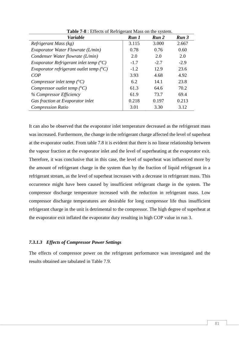
81
Table 7-8 : Effects of Refrigerant Mass on the system.
Variable Run 1 Run 2 Run 3
Refrigerant Mass (kg) 3.115 3.000 2.667
Evaporator Water Flowrate (L/min) 0.78 0.76 0.60
Condenser Water flowrate (L/min) 2.0 2.0 2.0
Evaporator Refrigerant inlet temp (oC) -1.7 -2.7 -2.9
Evaporator refrigerant outlet temp (oC) -1.2 12.9 23.6
COP 3.93 4.68 4.92
Compressor inlet temp (oC) 6.2 14.1 23.8
Compressor outlet temp (oC) 61.3 64.6 70.2
% Compressor Efficiency 61.9 73.7 69.4
Gas fraction at Evaporator inlet 0.218 0.197 0.213
Compression Ratio 3.01 3.30 3.12
It can also be observed that the evaporator inlet temperature decreased as the refrigerant mass
was increased. Furthermore, the change in the refrigerant charge affected the level of superheat
at the evaporator outlet. From table 7.8 it is evident that there is no linear relationship between
the vapour fraction at the evaporator inlet and the level of superheating at the evaporator exit.
Therefore, it was conclusive that in this case, the level of superheat was influenced more by
the amount of refrigerant charge in the system than by the fraction of liquid refrigerant in a
refrigerant stream, as the level of superheat increases with a decrease in refrigerant mass. This
occurrence might have been caused by insufficient refrigerant charge in the system. The
compressor discharge temperature increased with the reduction in refrigerant mass. Low
compressor discharge temperatures are desirable for long compressor life thus insufficient
refrigerant charge in the unit is detrimental to the compressor. The high degree of superheat at
the evaporator exit inflated the evaporator duty resulting in high COP value in run 3.
7.3.1.3 Effects of Compressor Power Settings
The effects of compressor power on the refrigerant performance was investigated and the
results obtained are tabulated in Table 7.9.
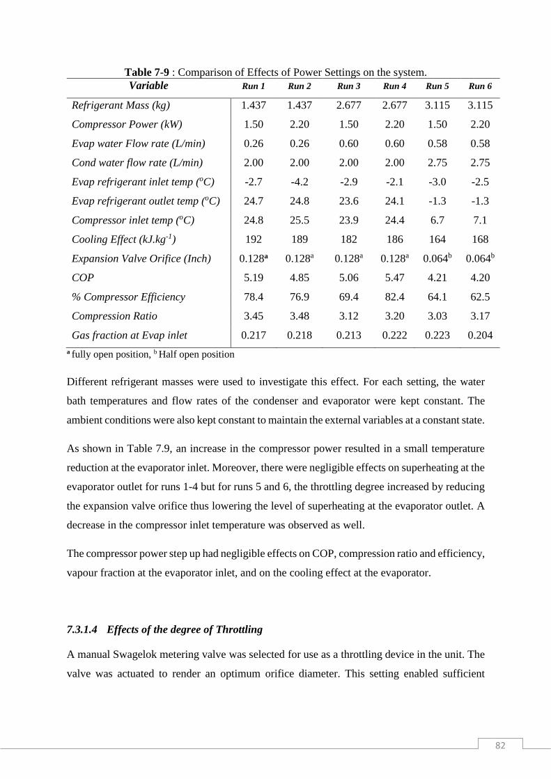
82
Table 7-9 : Comparison of Effects of Power Settings on the system.
Variable Run 1 Run 2 Run 3 Run 4 Run 5 Run 6
Refrigerant Mass (kg) 1.437 1.437 2.677 2.677 3.115 3.115
Compressor Power (kW) 1.50 2.20 1.50 2.20 1.50 2.20
Evap water Flow rate (L/min) 0.26 0.26 0.60 0.60 0.58 0.58
Cond water flow rate (L/min) 2.00 2.00 2.00 2.00 2.75 2.75
Evap refrigerant inlet temp (oC) -2.7 -4.2 -2.9 -2.1 -3.0 -2.5
Evap refrigerant outlet temp (oC) 24.7 24.8 23.6 24.1 -1.3 -1.3
Compressor inlet temp (oC) 24.8 25.5 23.9 24.4 6.7 7.1
Cooling Effect (kJ.kg-1) 192 189 182 186 164 168
Expansion Valve Orifice (Inch) 0.128a 0.128a 0.128a 0.128a 0.064b 0.064b
COP 5.19 4.85 5.06 5.47 4.21 4.20
% Compressor Efficiency 78.4 76.9 69.4 82.4 64.1 62.5
Compression Ratio 3.45 3.48 3.12 3.20 3.03 3.17
Gas fraction at Evap inlet 0.217 0.218 0.213 0.222 0.223 0.204
a fully open position, b Half open position
Different refrigerant masses were used to investigate this effect. For each setting, the water
bath temperatures and flow rates of the condenser and evaporator were kept constant. The
ambient conditions were also kept constant to maintain the external variables at a constant state.
As shown in Table 7.9, an increase in the compressor power resulted in a small temperature
reduction at the evaporator inlet. Moreover, there were negligible effects on superheating at the
evaporator outlet for runs 1-4 but for runs 5 and 6, the throttling degree increased by reducing
the expansion valve orifice thus lowering the level of superheating at the evaporator outlet. A
decrease in the compressor inlet temperature was observed as well.
The compressor power step up had negligible effects on COP, compression ratio and efficiency,
vapour fraction at the evaporator inlet, and on the cooling effect at the evaporator.
7.3.1.4 Effects of the degree of Throttling
A manual Swagelok metering valve was selected for use as a throttling device in the unit. The
valve was actuated to render an optimum orifice diameter. This setting enabled sufficient
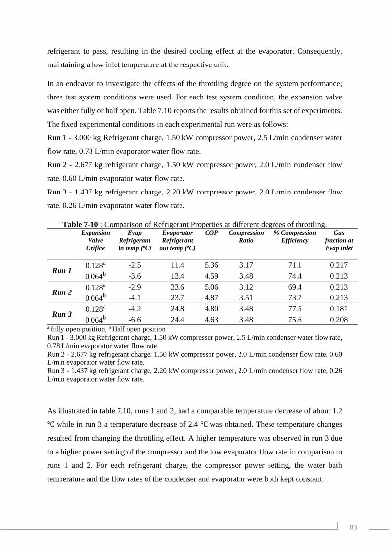
83
refrigerant to pass, resulting in the desired cooling effect at the evaporator. Consequently,
maintaining a low inlet temperature at the respective unit.
In an endeavor to investigate the effects of the throttling degree on the system performance;
three test system conditions were used. For each test system condition, the expansion valve
was either fully or half open. Table 7.10 reports the results obtained for this set of experiments.
The fixed experimental conditions in each experimental run were as follows:
Run 1 - 3.000 kg Refrigerant charge, 1.50 kW compressor power, 2.5 L/min condenser water
flow rate, 0.78 L/min evaporator water flow rate.
Run 2 - 2.677 kg refrigerant charge, 1.50 kW compressor power, 2.0 L/min condenser flow
rate, 0.60 L/min evaporator water flow rate.
Run 3 - 1.437 kg refrigerant charge, 2.20 kW compressor power, 2.0 L/min condenser flow
rate, 0.26 L/min evaporator water flow rate.
Table 7-10 : Comparison of Refrigerant Properties at different degrees of throttling.
Expansion
Valve
Orifice
Evap
Refrigerant
In temp (oC)
Evaporator
Refrigerant
out temp (oC)
COP
Compression
Ratio
% Compression
Efficiency
Gas
fraction at
Evap inlet
Run 1 0.128a -2.5 11.4 5.36 3.17 71.1 0.217
0.064b -3.6 12.4 4.59 3.48 74.4 0.213
Run 2 0.128a -2.9 23.6 5.06 3.12 69.4 0.213
0.064b -4.1 23.7 4.87 3.51 73.7 0.213
Run 3 0.128a -4.2 24.8 4.80 3.48 77.5 0.181
0.064b -6.6 24.4 4.63 3.48 75.6 0.208 a fully open position, b Half open position
Run 1 - 3.000 kg Refrigerant charge, 1.50 kW compressor power, 2.5 L/min condenser water flow rate,
0.78 L/min evaporator water flow rate.
Run 2 - 2.677 kg refrigerant charge, 1.50 kW compressor power, 2.0 L/min condenser flow rate, 0.60
L/min evaporator water flow rate.
Run 3 - 1.437 kg refrigerant charge, 2.20 kW compressor power, 2.0 L/min condenser flow rate, 0.26
L/min evaporator water flow rate.
As illustrated in table 7.10, runs 1 and 2, had a comparable temperature decrease of about 1.2
℃ while in run 3 a temperature decrease of 2.4 ℃ was obtained. These temperature changes
resulted from changing the throttling effect. A higher temperature was observed in run 3 due
to a higher power setting of the compressor and the low evaporator flow rate in comparison to
runs 1 and 2. For each refrigerant charge, the compressor power setting, the water bath
temperature and the flow rates of the condenser and evaporator were both kept constant.
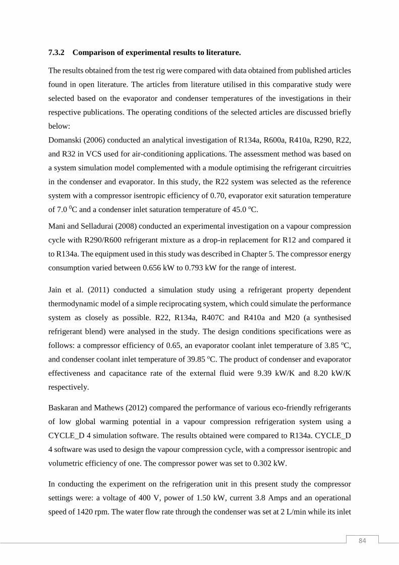
84
7.3.2 Comparison of experimental results to literature.
The results obtained from the test rig were compared with data obtained from published articles
found in open literature. The articles from literature utilised in this comparative study were
selected based on the evaporator and condenser temperatures of the investigations in their
respective publications. The operating conditions of the selected articles are discussed briefly
below:
Domanski (2006) conducted an analytical investigation of R134a, R600a, R410a, R290, R22,
and R32 in VCS used for air-conditioning applications. The assessment method was based on
a system simulation model complemented with a module optimising the refrigerant circuitries
in the condenser and evaporator. In this study, the R22 system was selected as the reference
system with a compressor isentropic efficiency of 0.70, evaporator exit saturation temperature
of 7.0 0C and a condenser inlet saturation temperature of 45.0 oC.
Mani and Selladurai (2008) conducted an experimental investigation on a vapour compression
cycle with R290/R600 refrigerant mixture as a drop-in replacement for R12 and compared it
to R134a. The equipment used in this study was described in Chapter 5. The compressor energy
consumption varied between 0.656 kW to 0.793 kW for the range of interest.
Jain et al. (2011) conducted a simulation study using a refrigerant property dependent
thermodynamic model of a simple reciprocating system, which could simulate the performance
system as closely as possible. R22, R134a, R407C and R410a and M20 (a synthesised
refrigerant blend) were analysed in the study. The design conditions specifications were as
follows: a compressor efficiency of 0.65, an evaporator coolant inlet temperature of 3.85 oC,
and condenser coolant inlet temperature of 39.85 oC. The product of condenser and evaporator
effectiveness and capacitance rate of the external fluid were 9.39 kW/K and 8.20 kW/K
respectively.
Baskaran and Mathews (2012) compared the performance of various eco-friendly refrigerants
of low global warming potential in a vapour compression refrigeration system using a
CYCLE_D 4 simulation software. The results obtained were compared to R134a. CYCLE_D
4 software was used to design the vapour compression cycle, with a compressor isentropic and
volumetric efficiency of one. The compressor power was set to 0.302 kW.
In conducting the experiment on the refrigeration unit in this present study the compressor
settings were: a voltage of 400 V, power of 1.50 kW, current 3.8 Amps and an operational
speed of 1420 rpm. The water flow rate through the condenser was set at 2 L/min while its inlet

85
temperature was varied while the water inlet to the evaporator was maintained at 25 oC, its
flowrate was adjusted to give the desired level of superheating of the refrigerant at the
evaporator outlet. The refrigerant inlet temperature to the evaporator was controlled by
adjusting the throttling effect at the expansion valves.
Table 7.11 shows a comparison of the data taken from literature sources and the results obtained
from the measurements performed on the refrigerant test rig in this study. The reference
conditions are the evaporator and condenser temperatures, and the resultant values at specific
points are compared.
Table 7-11 : Comparison of Experimental results to literature for R134a with Evaporator (4-5 oC) and Condenser (40 oC).
Variable (Mani and
Selladurai,
2008)
(Donald et al.,
1997)
(Domanski,
2006)
(Jain et al.,
2011)
(Baskaran
and
Mathews,
2012)
Run 1 from
the test rig in
this study
Evap/Cond Temp (oC) 2/40 3.85/36.85 7/45.6 3.85/39.85 -10/50 4.75/41.4
Evap Press (kPa) 345 336 365 250 200 320
Cond Press (kPa) 1003 934 1160 1314 1317 1113
Compression Ratio 2.91 2.78 3.14 5.26 6.57 3.65
Refrigeration Effect
(kJ.kg-1) 145 149 * 124 137 152
Wcomp ( kJ.kg-1) * * * 54 41. 45
Isentropic Efficiency * * 0.701 0.65 * 0.60
COP 2.34 * * 2.31 3.32 3.38
*Data for the empty spaces was not documented in the respective publications.
From the results tabulated in Table 7.11, it can be observed that the condenser and evaporator
pressures in literature are comparable to the data obtained from the test rig designed for this
study. Furthermore, the compression ratio from the test rig falls within the range of the values
reported in literature. The COP value from the test rig was higher than the literature values due
to the uncontrolled level of superheating at the evaporator outlet in the test rig. However it was
within the uncertainty of 16.8% as reported by Hoşöz (2005) using the uncertainty function R
computed by Moffat.
Overall, from Table 7.11, it is evident that the results obtained from the experiments conducted
on the unit were comparable to literature data. This outcome validates the design, equipment

86
assembly and experimental technique as accurate and reliable, and confirms the suitability of
the equipment for use in conducting the experimental work in this study.
The compressor, which is the driving force in the vapour compression system, operated within
the range of allowable temperatures that are safe for its components and lubricating oil. The
degree of throttling produced at the expansion valve was adequate to influence the refrigeration
effect at the evaporator. However, it was inconclusive that the same throttling effect would be
reproduced with all refrigerants, as they require different degrees of throttling to produce the
same refrigeration effect (Emerson, 1969).
The evaporator-compressor-condenser balance was satisfactory in the test rig using R134a.
That is, the refrigerant vapour generated in the evaporator, was sufficiently compressed and
displaced at the compressor, in the vapour phase. It condensed in the condenser to the required
level of sub-cooling. If this balance was not satisfied, the refrigeration effect would limited,
and as a result the compressor life will be shortened, making the cycle difficult to operate.
7.4 Performance analysis of refrigerants R413a, R507a and R134a.
The experimental performance of two commercial blends R413a and R507a was analysed and
compared to that of R134a (a pure refrigerant). Moreover, the performance of the test rig was
critically assessed in the investigation. However, the presence of auxiliary components and
connecting pipes made it difficult to represent any practical refrigeration cycle purely based on
a single parameter without the effects of the other parameters. Additionally, there was a limited
number of measurement points with conventional sensors for pressure and temperature; this
was due to the physical constraints on the system. (Datta et al., 2014). Hence, in this unit due
to the lack of pressure sensors at the expansion valve, the pressure readings at its outlet were
assumed to be equal to that of the evaporator inlet. This assumption was made so that a
simplified representation of the thermodynamic cycle depicted by the system was a possibility.
The investigation on refrigerant R507 on the test unit was limited since it is a high- pressure
refrigerant and the unit utilised in this study had an upper pressure limit of 1.9 MPa. Parameters
of interest in this analysis were the amount of refrigerant charge, condenser and evaporator
water flow rates, evaporator temperatures, and condenser temperatures, compressor discharge
temperature, cooling effect, COP compressor work and efficiency.

87
7.4.1 Variation of Compressor Work with COP
The Coefficient of Performance (COP) is defined as the ratio of cooling effect to compressor
work. Consequently, an inverse proportionality relationship was expected when COP was
plotted against compressor work. The expected trend was obtained and is shown below in
Figure 7.1.
Figure 7-1 : Compressor Work vs. Coefficient of performance (COP). (*) R507, (▲) R413a,
(●) R134a.
For the pure refrigerant R134a and refrigerant blend R507a (R125/R143a, 50/50 wt %) the
COP decreased as the compressor work increased. The departure from linearity of the plot was
because of the influence of the surroundings on the system. R404 a ternary blend showed the
same behavior (Jerald and Kumaran, 2014). In this case, the departure from linearity was due
to the influence of the other parameters such as oil circulation, temperature fluctuations in the
condenser bath and influence of the environment on the system (heat loss to the environment).
7.4.2 Variation of Evaporator Temperature with COP
Extensive studies have been done and published on the variation of COP with evaporator
temperature for various refrigerants investigated. The variation of evaporator temperature with
COP for this study is shown below in Figure 7.2. It is evident from Figure 7.2 that the increase
in evaporator temperature leads to an increase in COP.
3,5
3,7
3,9
4,1
4,3
4,5
4,7
4,9
5,1
5,3
5,5
32 34 36 38 40 42 44
Co
effi
cien
t o
f p
erfo
rma
nce
(C
OP
)
Compressor Work (kJ/kg)
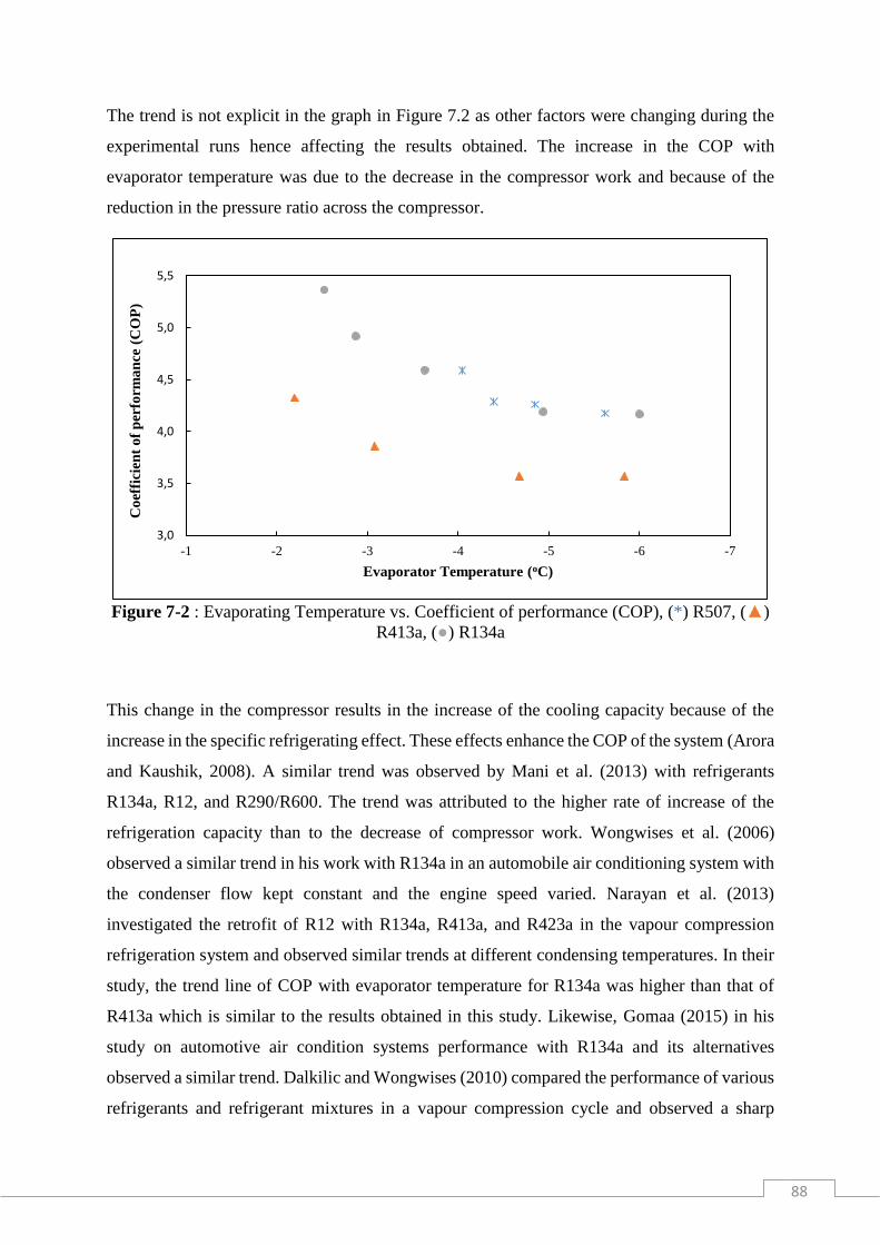
88
The trend is not explicit in the graph in Figure 7.2 as other factors were changing during the
experimental runs hence affecting the results obtained. The increase in the COP with
evaporator temperature was due to the decrease in the compressor work and because of the
reduction in the pressure ratio across the compressor.
Figure 7-2 : Evaporating Temperature vs. Coefficient of performance (COP), (*) R507, (▲)
R413a, (●) R134a
This change in the compressor results in the increase of the cooling capacity because of the
increase in the specific refrigerating effect. These effects enhance the COP of the system (Arora
and Kaushik, 2008). A similar trend was observed by Mani et al. (2013) with refrigerants
R134a, R12, and R290/R600. The trend was attributed to the higher rate of increase of the
refrigeration capacity than to the decrease of compressor work. Wongwises et al. (2006)
observed a similar trend in his work with R134a in an automobile air conditioning system with
the condenser flow kept constant and the engine speed varied. Narayan et al. (2013)
investigated the retrofit of R12 with R134a, R413a, and R423a in the vapour compression
refrigeration system and observed similar trends at different condensing temperatures. In their
study, the trend line of COP with evaporator temperature for R134a was higher than that of
R413a which is similar to the results obtained in this study. Likewise, Gomaa (2015) in his
study on automotive air condition systems performance with R134a and its alternatives
observed a similar trend. Dalkilic and Wongwises (2010) compared the performance of various
refrigerants and refrigerant mixtures in a vapour compression cycle and observed a sharp
3,0
3,5
4,0
4,5
5,0
5,5
-7-6-5-4-3-2-1
Co
effi
cien
t o
f p
erfo
rma
nce
(C
OP
)
Evaporator Temperature (oC)

89
increase in COP as the evaporator temperature increased. Additionally, Halimic et al. (2003),
presented a similar nonlinear trend in his comparison of the operating performance of
alternative refrigerants and attributed it to the difference between equipment design and the
experimental construction of the unit.
7.4.3 Variation of Condenser Temperature with Compressor Work
The compressor work varies directly with the condensing temperature of the refrigerants. This
variation was due to the fact that the high condensing temperature led to a higher pressure ratio
which resulted in high compressor work (Hwang et al., 2004). Hence more work was done in
the compressor as it compressed the low-pressure gas to a high-pressure state. This variation is
shown in Figure 7.3 with two refrigerants R134a and R413a.
Figure 7-3 : Condensing Temperature vs. Compressor Work, (▲) R413a, (●) R134a
The trends obtained with these two refrigerants were the same, with refrigerant R413a
operating at a lower condenser temperature than refrigerant R134a due to lower compressor
work in the R413a system. This observation might have been due to good miscibility between
R413a and the lubrication oil which led to less frictional work in the compressor hence low
compressor discharge temperatures. Therefore, R413a performs better than R134a in the unit
with regards to compressor operation and compressor life.
25
30
35
40
45
50
15 20 25 30 35 40
Co
mp
ress
or
Wo
rk (
kJ
/Kg
)
Condensing Temperature (oC)

90
7.4.4 Variation of Condenser Temperature with COP
Figure 7.4 shows the variation of COP with condensing temperature. From the figure, it is
apparent that COP was inversely proportional to the refrigerants’ condensing temperature.
Figure 7-4 : Condensing Temperature vs. Coefficient of performance (COP), (▲) R413a, (●)
R134a.
This observed trend was due to the decrease in refrigerating capacity and increase in the
compressor work (Mani et al., 2013). Additionally, high condensing temperature leads to high-
pressure ratio, which increased the power consumption of the compressor (high compressor
work) thus resulting in a reduction of COP (Elsayed and Hariri, 2011; Prapainop and Suen,
2012). Similar trends were observed by Mani et al. (2013), in the study of R12, R134a and
R290/R600 for the development of the statistical model for predicting refrigerant performance
as well as Elsayed and Hariri (2011), investigating the effects of condenser air flow on the
performance of split air conditioner. This trend was the same as the one obtained in this study
as illustrated in Figure 7.4. The commercial refrigerant R413a exhibited better performance
than pure refrigerant R134a, as R413a has a higher COP value for a lower condensing
temperature.
Hwang et al. (2004) in their study working with R-290, R404a and R410a in medium
temperature applications observed that at very low condensing temperatures, low COP was
obtained. COP increased with an increase in condenser temperature until it reached a maximum
3,0
3,5
4,0
4,5
5,0
5,5
6,0
15 20 25 30 35 40 45
Co
effi
cien
t o
f p
erfo
ma
nce
(C
OP
)
Condensing Temperature (oC)
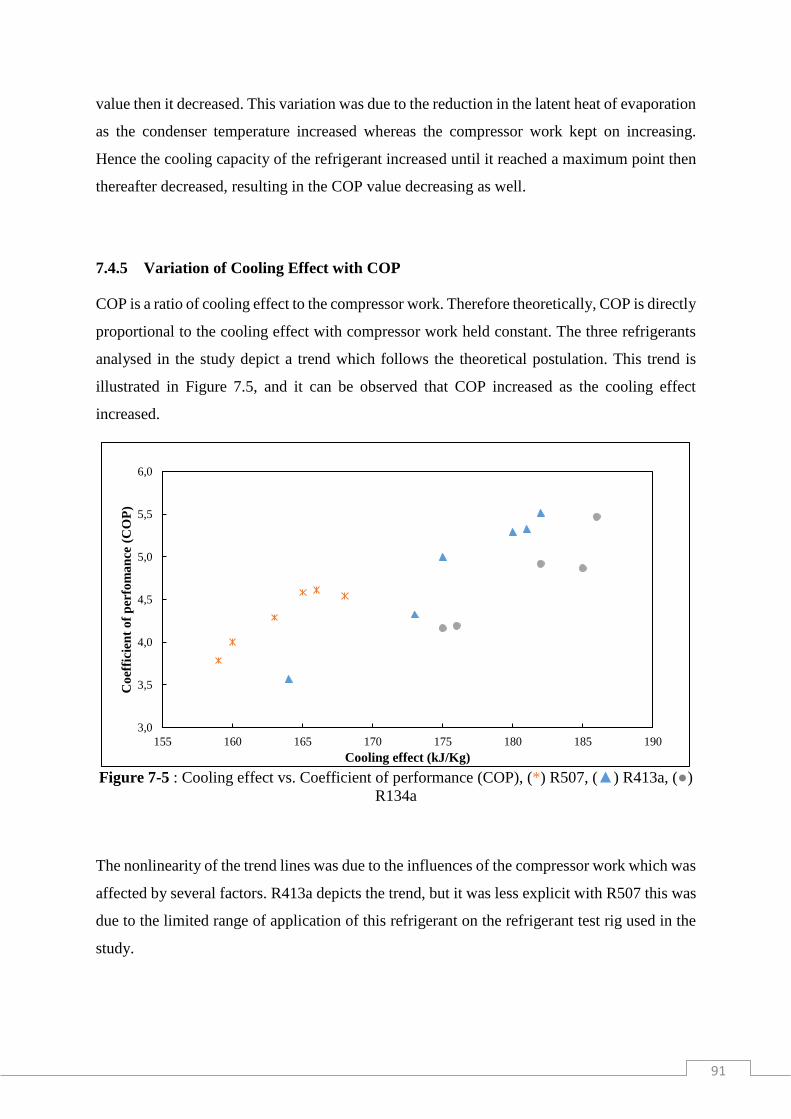
91
value then it decreased. This variation was due to the reduction in the latent heat of evaporation
as the condenser temperature increased whereas the compressor work kept on increasing.
Hence the cooling capacity of the refrigerant increased until it reached a maximum point then
thereafter decreased, resulting in the COP value decreasing as well.
7.4.5 Variation of Cooling Effect with COP
COP is a ratio of cooling effect to the compressor work. Therefore theoretically, COP is directly
proportional to the cooling effect with compressor work held constant. The three refrigerants
analysed in the study depict a trend which follows the theoretical postulation. This trend is
illustrated in Figure 7.5, and it can be observed that COP increased as the cooling effect
increased.
Figure 7-5 : Cooling effect vs. Coefficient of performance (COP), (*) R507, (▲) R413a, (●)
R134a
The nonlinearity of the trend lines was due to the influences of the compressor work which was
affected by several factors. R413a depicts the trend, but it was less explicit with R507 this was
due to the limited range of application of this refrigerant on the refrigerant test rig used in the
study.
3,0
3,5
4,0
4,5
5,0
5,5
6,0
155 160 165 170 175 180 185 190
Co
effi
cien
t o
f p
erfo
ma
nce
(C
OP
)
Cooling effect (kJ/Kg)
92
7.4.6 Variation of Condenser Water Flowrate effect with COP
The relationship between condenser water flowrate and COP for pure refrigerant R134a and
refrigerant blend R507 is shown in Figure 7.6, where the performance of the two refrigerants
investigated was in a comparable range. Considering refrigerant blend R507 it is evident that
initially COP increased with condenser water flow rate until a maximum value was reached
thereafter COP decreased as the condenser flow rate increased at a low flowrate.
Figure 7-6 : Condenser Water flowrate vs. Coefficient of performance (COP), (▲) R507, (●)
R134a
With refrigerant R134a, the COP decreased as the condenser flowrate increased. However, it
may be the case that the R134a graph is similar to the second part of the R507 graph. Cooling
of the refrigerant was affected when the condenser was starved of the cooling fluid (Datta et
al., 2014).
7.4.7 Variation of Condenser water flowrate with Discharge Temperature
Datta et al. (2014) in the study on automobile air-conditioning observed that starving the
condenser of the airflow (heat sink) leads to a decrease in the cooling of the refrigerant through
it. Likewise, an increase in the condenser cooling water flowrate with its temperature held
constant leads to improved refrigerant cooling. The throttling effect becomes more pronounced
at the expansion valve. This throttling effect leads to excellent cooling which results in lower
3,0
3,2
3,4
3,6
3,8
4,0
4,2
4,4
4,6
4,8
1,5 2,0 2,5 3,0 3,5 4,0
Co
effi
cien
t o
f p
erfo
rma
nce
(C
OP
)
Condenser Water flowrate (L/min)
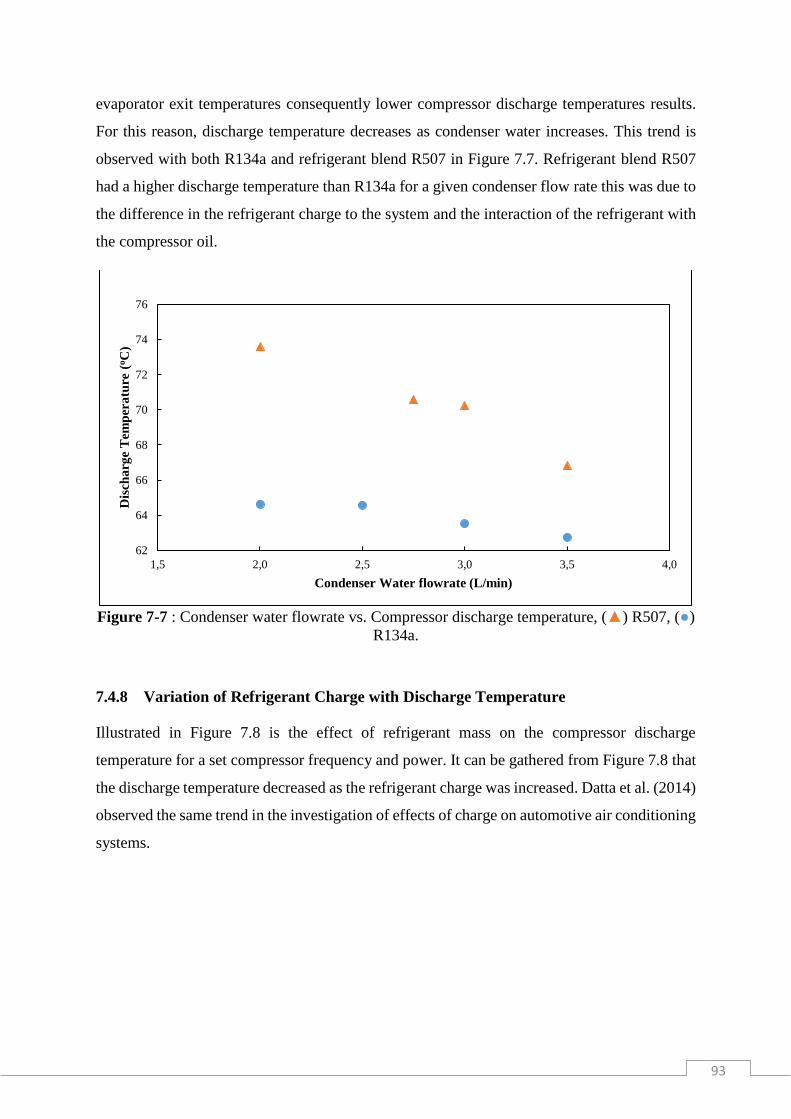
93
evaporator exit temperatures consequently lower compressor discharge temperatures results.
For this reason, discharge temperature decreases as condenser water increases. This trend is
observed with both R134a and refrigerant blend R507 in Figure 7.7. Refrigerant blend R507
had a higher discharge temperature than R134a for a given condenser flow rate this was due to
the difference in the refrigerant charge to the system and the interaction of the refrigerant with
the compressor oil.
Figure 7-7 : Condenser water flowrate vs. Compressor discharge temperature, (▲) R507, (●)
R134a.
7.4.8 Variation of Refrigerant Charge with Discharge Temperature
Illustrated in Figure 7.8 is the effect of refrigerant mass on the compressor discharge
temperature for a set compressor frequency and power. It can be gathered from Figure 7.8 that
the discharge temperature decreased as the refrigerant charge was increased. Datta et al. (2014)
observed the same trend in the investigation of effects of charge on automotive air conditioning
systems.
62
64
66
68
70
72
74
76
1,5 2,0 2,5 3,0 3,5 4,0
Dis
cha
rge
Tem
per
atu
re (
oC
)
Condenser Water flowrate (L/min)

94
Figure 7-8 : Refrigerant charge vs. compressor discharge temperature, (▲) R413a, (●)
R134a
7.4.9 Variation of Refrigerant Charge with Compressor Efficiency
Figure 7.9 shows the variation of refrigerant mass with the compressor efficiency. It can be
observed that compressor efficiency decreased as the refrigerant charge was increased for
R134a refrigerant. This change was as a result of the increase of vapour compressed in the
Figure 7-9 : Refrigerant charge vs Compressor Efficiency, (▲) R413a, (●) R134a.
60
61
62
63
64
65
66
67
68
69
0,5 1,0 1,5 2,0 2,5 3,0 3,5
Dis
cha
rge
Tem
per
atu
re (
oC
)
Refrigerant Charge (kg)
0,50
0,55
0,60
0,65
0,70
0,75
0,80
0,5 1,0 1,5 2,0 2,5 3,0 3,5 4,0
Co
mp
ress
or
Eff
icie
ncy
Refrigerant Charge (Kg)
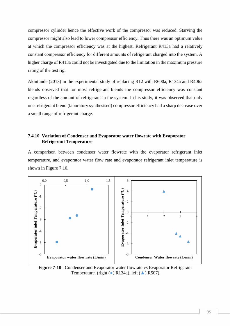
95
compressor cylinder hence the effective work of the compressor was reduced. Starving the
compressor might also lead to lower compressor efficiency. Thus there was an optimum value
at which the compressor efficiency was at the highest. Refrigerant R413a had a relatively
constant compressor efficiency for different amounts of refrigerant charged into the system. A
higher charge of R413a could not be investigated due to the limitation in the maximum pressure
rating of the test rig.
Akintunde (2013) in the experimental study of replacing R12 with R600a, R134a and R406a
blends observed that for most refrigerant blends the compressor efficiency was constant
regardless of the amount of refrigerant in the system. In his study, it was observed that only
one refrigerant blend (laboratory synthesised) compressor efficiency had a sharp decrease over
a small range of refrigerant charge.
7.4.10 Variation of Condenser and Evaporator water flowrate with Evaporator
Refrigerant Temperature
A comparison between condenser water flowrate with the evaporator refrigerant inlet
temperature, and evaporator water flow rate and evaporator refrigerant inlet temperature is
shown in Figure 7.10.
Figure 7-10 : Condenser and Evaporator water flowrate vs Evaporator Refrigerant
Temperature. (right (●) R134a), left (▲) R507)
-6
-5
-4
-3
-2
-1
0
0,0 0,5 1,0 1,5
Ev
ap
ora
tor
inle
t T
emp
era
ture
(oC
)
Evaporator water flow rate (L/min)-8
-6
-4
-2
0
2
4
6
0 1 2 3 4
Ev
ap
ora
tor
Inle
t T
emp
era
ture
(oC
)
Condenser Water flowrate (L/min)

96
The refrigerant temperature at the evaporator inlet decreased with an increase in condenser
water flowrate conversely it increased with the evaporator water flowrate. An increase in the
condenser water flowrate increases the rate of heat rejection at the heat sink thus the refrigerant
emerges with a lower temperature thus the throttling effect produced a vapour liquid mixture
with higher liquid fraction which led to a lower temperature at the evaporator inlet.
At high evaporator temperatures, the amount of superheat was high hence the refrigerant exited
the evaporator at higher temperature. Heat rejection was constant at the condenser since the
condenser conditions were kept constant. Therefore, the outlet temperature of the refrigerant at
the condenser increased with the increase in the flow rate through the evaporator.
Consequently, the refrigerant returned to the evaporator at a higher temperature.
7.5 Simulations for the Vapour Compression Cycle
COND CONDENSER
COMP COMPRESSOR
EVAP EVAPORATOR
EXV EXPANSION VALVE
CW-IN CONDENSER WATER INLET
CW-OUT CONDENSER WATER OUTLET
EW-IN EVAPORATOR WATER INLET
EW-OUT EVAPORATOR WATER OUTLET
S1 REFRIGERANT STREAM 1
S2 REFRIGERANT STREAM 2
S3 REFRIGERANT STREAM 3
S4 REFRIGERANT STREAM 4
Figure 7-11 : Flowsheet of a single vapour compression cycle with Hot and Cold fluid
cycles.
EV AP
COND
COMPEXV
S1
S2
S3
S4
EW-IN
EW-OUT
CW-IN
CW-OUT

97
Aspen Plus ® V8.6 an engineering software was employed to simulate of the refrigeration cycle,
the results obtained were compared to the results obtained from the experimental study. Figure
7.11 presents the simulated cycle developed using Aspen Plus ®. The simulation model consists
of the four main components of a VC cycle, which are; the evaporator, the compressor, an
expansion valve, a condenser, the connecting lines and water lines.
7.5.1 Components Selection for the vapour compression cycle
The unit operations forming the refrigeration cycle are the condenser, the evaporator, the
compressor and an expansion valve. The evaporator and the condenser selected from the
Exchangers, under the HeatX category, and of the Gen HT type this type chosen because it best
simulates the evaporator and condenser used in the refrigerant test unit, with two inlet and
outlet ports.
The compressor was selected from Pressure changers, under the Compr category and the
ICON2 type. This simulated the reciprocating compressor utilised in the refrigerant test rig.
Similarly, the expansion valve was selected from Pressure changers, in the Valves category.
Specifically, VALVE2 was chosen as it best simulated the throttling effect produced by the
expansion valve in the refrigerant unit.
Material lines were used to connect the various units in the sequence as shown in Figure 7.11.
7.5.2 Thermodynamics models employed in the study
REPROF (REFerence fluid PROPerties package) method was utilised in evaluating the
simulation performance the refrigeration cycle in this study. This method has been used
successfully in refrigeration studies by, (Kim and Didion, 1995); (Satola, 2014), and (Tuta and
Orozco, 2016).
REPROF was developed by NIST and contains 121 pure fluids some of which are binary
mixtures. Its particular emphasis is on refrigerants and hydrocarbons. The REFPROP package
describes fluids properties with an uncertainty of below 1% for most conditions (Satola, 2014).
It is based on three accurate thermodynamics models for pure liquids and mixtures. It
implements these models for the thermodynamic properties of pure fluids: the Modified
Benedict-Webb-Rubin equation of state, Equations of State (EoS) explicit in Helmholtz energy
and an extended corresponding states (ECS) model.

98
The fundamental equation of state explicit in the Helmholtz free energy f has the independent
variables which are temperature T and density ρ. Several thermodynamics properties can be
obtained from the Helmholtz free energy equation derivate (Equation 7.1) as a function of these
two variables. Also, it is one of the four fundamental equations of state (Wagner and Pruß,
2002).
𝜙(𝛿, 𝜏) = 𝜙𝑜(𝛿, 𝜏) + 𝜙𝑟(𝛿, 𝜏), (7.1)
where 𝜏 = 𝑇𝑐 / 𝑇 is the inverted reduced temperature and 𝛿= 𝜌/𝜌𝑐 is the reduced density
with 𝑇𝑐 and 𝜌𝑐 being the critical temperature and critical density respectively. The fundamental
equation of state was established for Helmholtz free energy of refrigerant R134a by (Tillner-
Roth and Baehr, 1994). Its temperature range is from -103.15 to 181.85 oC with pressure of up
to 700 bars.
The modified Benedict-Webb-Rubin (mBWR) equation as described by Jacobsen and Stewart
(1973), it is very accurate and flexible to be applied to the liquid, vapour and supercritical
regions of the fluid. The mBWR equation represents the pressure P as a function of molar
density ρ and the absolute temperature T:
𝑃 = ∑ 𝑎𝑛
9
𝑛=1
𝜌𝑛 + exp(−𝛿𝑛) ∑ 𝑎𝑛
15
𝑛=10
𝜌2𝑛−17 (7.2)
where 𝛿=𝜌/𝜌𝑐, 𝜌𝑐 is the critical density, and the temperature dependence of the coefficients is
given by Outcalt and McLinden (1996). The data covers the temperature range from -103.15
to 251.85 oC with pressure of up to 350 bars in terms of the mBWR equation of state with 32
adjustable coefficients with refrigerant R152a (Outcalt and McLinden, 1996).
The Extended Corresponding-States Principle (ECS) is used to represent transport properties
and thermodynamic of fluid with particular emphasis on fluids with limited data. This principle
does not depend on the assumption that molecules are symmetric spheres with conformal
intermolecular potentials as some refrigerants have non-spherical and polar molecules. The
shapes factors of these substances are reduced and represented as functions of density and

99
temperature (Ely and Huber, 1990). This method was found to work well with R134a reference
fluid for various fluids (McLinden et al., 2000). Furthermore, the implementation of extended
corresponding states requires the molecular mass, critical point, and normal boiling point to be
specified as these empirical relations can be used to obtain the shape factors (Huber et al.,
1992).
In mixture calculations, a different rule applies which combines the Helmholtz energy of the
components in the mixture; and a difference function is used to account for the deviation from
ideal mixing. Thermal conductivity and viscosity modeled with either fluid-specific
correlations, an ECS method or the friction theory method in some cases. REFPROP has three
reference states on which the values of entropy and enthalpy are based. The analysis of the
mixtures is also made complex by the composition of the equivalent substance reducing ratios.
To simplify the system, an assumption is made that the composition dependence is offered by
the van der Waals one-fluid mixing rules. The following equations illustrate the van der Waals
mixing rules:
ℎ𝑥 = ∑ ∑ 𝑥𝑖𝑥𝑗
𝑛
𝑗=1
𝑛
𝑖=1
ℎ𝑖𝑗
7.3
𝑓𝑥ℎ𝑥 = ∑ ∑ 𝑥𝑖
𝑛
𝑗=1
𝑛
𝑖=1
𝑥𝑗𝑓𝑖𝑗ℎ𝑖𝑗 7.4
The cross terms obtained from combining rules are;
𝑓𝑖𝑗 = √𝑓𝑖𝑓𝑗(1 − 𝑘𝑖𝑓)
7.5
ℎ𝑖𝑗 = (ℎ𝑖1 3⁄
+ ℎ𝑗1 3⁄
)3
(1 − 𝑙𝑖𝑗)/8
7.6

100
where 𝑥𝑖 is the concentration of constituent i in the mixture, 𝑘𝑖𝑗 and 𝑙𝑖𝑗 are the binary interaction
parameters and are nonzero when 𝑖 ≠ 𝑗 also ℎ𝑥 and 𝑓𝑥 are the equivalent substance reducing
ratios for the mixture (Ely and Huber, 1990). Application of the mixing formulas requires the
derivatives of ℎ𝑥 and 𝑓𝑥 with respect to composition, density and temperature. The arguments
of the shape factors pertaining to the mixing rules and the definition of equivalence substance
reducing ratios are shown to be the effective temperature and densities of the mixture’s
components. The scope of equations of state described here have been limited due to the
substances covered in this study.
7.5.3 Specifications of Simulation Parameters
In running the simulation software, there was a need to specify variables for each component
and stream shown in Figure 7.11. The simulation model computed the unspecified variables.
The methodology of variable specification used is detailed in Table 7.12.
The inputs values used in the simulation were obtained from the experimental runs conducted
in the test rig used in this study. The results obtained from the simulations were then compared
with the experimental results to ascertain the deviation of experimental results from simulated
results (ideal).
The model computes the properties of the refrigeration streams as they flow around the cycle.
The outputs obtained were; enthalpy, entropy, density, liquid-vapour compositions,
unspecified temperatures and pressure for the refrigerant and water streams. Typical results
obtained from the simulation are presented in Appendix E, Table E.1 to Table E.7.
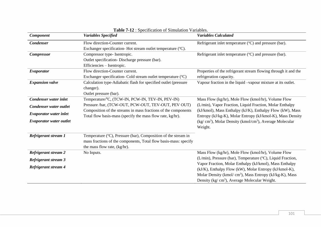
101
Table 7-12 : Specification of Simulation Variables. Component Variables Specified Variables Calculated
Condenser Flow direction-Counter current.
Exchanger specification- Hot stream outlet temperature (oC).
Refrigerant inlet temperature (oC) and pressure (bar).
Compressor Compressor type- Isentropic.
Outlet specification- Discharge pressure (bar).
Efficiencies – Isentropic.
Refrigerant inlet temperature (oC) and pressure (bar).
Evaporator Flow direction-Counter current.
Exchanger specification- Cold stream outlet temperature (oC)
Properties of the refrigerant stream flowing through it and the
refrigeration capacity.
Expansion valve Calculation type-Adiabatic flash for specified outlet (pressure
changer).
Outlet pressure (bar).
Vapour fraction in the liquid –vapour mixture at its outlet.
Condenser water inlet
Condenser water outlet
Evaporator water inlet
Evaporator water outlet
Temperature/0C, (TCW-IN, PCW-IN, TEV-IN, PEV-IN)
Pressure /bar, (TCW-OUT, PCW-OUT, TEV-OUT, PEV OUT)
Composition of the streams in mass fractions of the components
Total flow basis-mass (specify the mass flow rate, kg/hr).
Mass Flow (kg/hr), Mole Flow (kmol/hr), Volume Flow
(L/min), Vapor Fraction, Liquid Fraction, Molar Enthalpy
(kJ/kmol), Mass Enthalpy (kJ/K), Enthalpy Flow (kW), Mass
Entropy (kJ/kg-K), Molar Entropy (kJ/kmol-K), Mass Density
(kg/ cm3), Molar Density (kmol/cm3), Average Molecular
Weight.
Refrigerant stream 1 Temperature (oC), Pressure (bar), Composition of the stream in
mass fractions of the components, Total flow basis-mass: specify
the mass flow rate, (kg/hr).
Refrigerant stream 2
Refrigerant stream 3
Refrigerant stream 4
No Inputs. Mass Flow (kg/hr), Mole Flow (kmol/hr), Volume Flow
(L/min), Pressure (bar), Temperature (oC), Liquid Fraction,
Vapor Fraction, Molar Enthalpy (kJ/kmol), Mass Enthalpy
(kJ/K), Enthalpy Flow (kW), Molar Entropy (kJ/kmol-K),
Molar Density (kmol/ cm3), Mass Entropy (kJ/kg-K), Mass
Density (kg/ cm3), Average Molecular Weight.

102
The pure refrigerants and refrigerants blends analysed were: R134a, R507, R413a, R134a/R125
(66/34 wt %), and R134a/R125 (50/50 wt %).
7.5.4 Analysis of the simulated results
The results obtained from Aspen simulations of two pure refrigerants and four refrigerant
blends are presented in Table 7.13.
Table 7-13 : Comparison of Simulated COP results for refrigerants and refrigerant blends.
Refrigerant/Refrigerant
Blend (wt %)
Compressor
Work (kW)
Refrigeration
Effect (kW)
COP
R134a 0.09 0.43 4.78
R413a
R134a/R600a/R218
(88/3/9)
0.09 0.36 4.00
R134a\R125
(50/50) 0.05 0.24 4.80
R134a\R125
(66/34) 0.07 0.34 4.86
R507
R143a/R125
(50/50)
0.08 0.40 5.0
R125 0.07 0.29 4.41
The commercial refrigerant blend R507 had the highest COP while R413a another commercial
blend had the lowest COP value. R134a, a pure refrigerant had the highest refrigeration effect
while R134a/R125 (50/50) had the lowest refrigeration effect as well as the compressor work.
The high COP value for R507 was a result of both relatively high refrigeration effect and low
power consumption at the compressor. Moreover, the high COP might have been due to high
volumetric refrigeration capacity of the R507 refrigerant as a result of the high pressure of its
vapour since it had the highest pressure in the study (Prapainop and Suen, 2012). R134a/R125
(66/34 wt %) a laboratory synthesised blend in this study had the second highest COP value.
The overall performance of refrigeration blends was better than that of pure refrigerants in the
simulation, with R125 a pure refrigerant gave the lowest COP value. R507 a commercial blend
of R125/R143a in the ratio (50/50) showed better performance when compared to R134a/R125
in the same proportion.
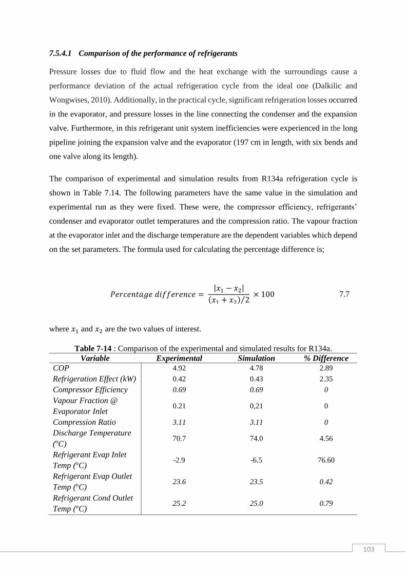
103
7.5.4.1 Comparison of the performance of refrigerants
Pressure losses due to fluid flow and the heat exchange with the surroundings cause a
performance deviation of the actual refrigeration cycle from the ideal one (Dalkilic and
Wongwises, 2010). Additionally, in the practical cycle, significant refrigeration losses occurred
in the evaporator, and pressure losses in the line connecting the condenser and the expansion
valve. Furthermore, in this refrigerant unit system inefficiencies were experienced in the long
pipeline joining the expansion valve and the evaporator (197 cm in length, with six bends and
one valve along its length).
The comparison of experimental and simulation results from R134a refrigeration cycle is
shown in Table 7.14. The following parameters have the same value in the simulation and
experimental run as they were fixed. These were, the compressor efficiency, refrigerants’
condenser and evaporator outlet temperatures and the compression ratio. The vapour fraction
at the evaporator inlet and the discharge temperature are the dependent variables which depend
on the set parameters. The formula used for calculating the percentage difference is;
𝑃𝑒𝑟𝑐𝑒𝑛𝑡𝑎𝑔𝑒 𝑑𝑖𝑓𝑓𝑒𝑟𝑒𝑛𝑐𝑒 = |𝑥1 − 𝑥2|
(𝑥1 + 𝑥2) 2⁄ × 100 7.7
where 𝑥1 and 𝑥2 are the two values of interest.
Table 7-14 : Comparison of the experimental and simulated results for R134a.
Variable Experimental Simulation % Difference
COP 4.92 4.78 2.89
Refrigeration Effect (kW) 0.42 0.43 2.35
Compressor Efficiency 0.69 0.69 0
Vapour Fraction @
Evaporator Inlet 0.21 0,21 0
Compression Ratio 3.11 3.11 0
Discharge Temperature
(oC) 70.7 74.0 4.56
Refrigerant Evap Inlet
Temp (oC) -2.9 -6.5 76.60
Refrigerant Evap Outlet
Temp (oC) 23.6 23.5 0.42
Refrigerant Cond Outlet
Temp (oC) 25.2 25.0 0.79

104
The refrigeration capacity was higher in the simulated results than in the experiments. A
percentage difference of 2.35 % was observed between the experimental and theoretical study
as shown in Table 7.14. This was within the uncertainty of 16.8 % and 4.472 % calculated by
the uncertainty function R computed by Moffat (1988) as reported by Hoşöz (2005) and Datta
et al. (2014) respectively. The difference was mainly due to the inefficiencies which occur in
the experimental apparatus. The system inefficiencies were due to the loss of refrigeration
capacity to the surroundings, the section worth mentioning being the long pipeline that exists
between the expansion valve and the evaporator. The coefficient of performance was
unexpectedly higher for the experimental than for the theoretical run due to the compressor
effects and the exaggerated exit outlet evaporator temperature which increased the cooling
effect in the experimental run. A 2.91 % difference in COP existed between the measured and
simulated results. The inlet temperature of the evaporator was higher for the practical cycle
than the simulated one (Rigola et al., 1996). This occurrence was expected due to irreversibility
at the expansion valve in the practical cycle and the loss of the refrigeration capacity of the
refrigerant as it cooled (heat load) the long pipeline which connects the expansion valve and
the evaporator inlet. This section accounts for the large percentage difference that was observed
in the evaporator inlet temperature (76.6 %).
Table 7.15, shows the values obtained from the experimental and simulated runs for a
commercial refrigerant blend R507 under the same conditions. It can be noted that a difference
of 9.64 % existed between the COP values for the two methods with the experimental run
having a lower value.
Table 7-15 : Comparison of the Experimental and simulated results for R507.
Variables Experimental Simulation % Difference
COP 4.54 5.0 9.64
Refrigeration Effect (kW) 0.34 0.40 16.22
Compressor Efficiency 0.78 0.78 0
Vapour Fraction @
Evaporator Inlet 0.28 0.31 10.17
Compression Ratio 3.89 3.89 0
Discharge Temperature (oC) 71.4 79.2 10.36
Refrigerant Evap Inlet Temp
(oC) -5.9 -21.2 112.92
Refrigerant Evap Outlet
Temp (oC) 23.7 23.7 0
Refrigerant Cond Outlet
Temp (oC) 18.6 18.6 0

105
The percentage difference in COP between the experimental run and the simulation was small,
(within 10% difference), but the refrigeration effect was higher for the simulation than the
experimental run. As expected the COP value simulated results are greater than in the
experimental run. This observation was due to the inefficiencies that exist in the experimental
equipment. The percentage difference was within the 16.8% uncertainty computed by Hoşöz
(2005), using Moffat’s uncertainty function R.
Refrigerant R507 is a high-pressure refrigerant. Therefore, the test rig pressure limitations
affected its analysis, as a little amount of refrigerant R507 produced a high-pressure value. It
is also a low-temperature refrigerant, but the apex temperature it can reach is limited or
influenced by the external ambient temperature. The huge percentage difference of the
refrigerant temperature at the evaporator inlet was due to the fact that R507 is a higher-pressure
refrigerant. Thus its performance in the experimental unit was limited. Also, the systems’
inefficiencies affected the performance of the refrigerant in the unit.
Tabulated in Table 7.16 is the comparison of the experimental and simulated results obtained
with refrigerant blend R413a. Commercial R413a was intended to replace the Freon 12
refrigerant (R12). Therefore it was expected to have excellent refrigerant properties. As
expected the simulation produced better results than the experimental due to the effects of the
surroundings and system inefficiencies on the experimental runs.
Table 7-16 : Comparison of the experimental and simulated results for R413a.
Variables Experimental Simulation % Difference
COP 3.57 4.0 11.36
Refrigeration Effect (kW) 0.20 0.36 57.14
Compressor Efficiency 0.65 0.65 0
Vapour Fraction @ Evap
Inlet 0.22 0.23 4.44
Compression Ratio 3.79 3.80 0.26
Discharge Temperature (oC) 67.4 66.2 1.80
Refrigerant Evap Inlet Temp
(oC) -5.8 -8.0 31.88
Refrigerant Evap Outlet
Temp (oC) 6.9 6.9 0
Refrigerant Cond Outlet
Temp (oC) 23.9 23.9 0
The percentage difference in COP between the experimental result and the simulated results
was again less the 16.8 % uncertainty determined by Hoşöz (2005) using Moffat’s uncertainty

106
function (R). A higher compressor discharge temperature occurred in the experimental run due
to the inefficiency in the compressor, which generated much energy. This occurrence was a
result of some factors such as; friction between the moving parts in the compressor and the
incompatibility of the oil and the refrigerant investigated. One can observe that while the
difference in the values reported for the refrigeration effects is not huge, there is a significant
difference, in the inlet temperature of the evaporator which is attributed to the lengthy pipeline
between the expansion valve and the evaporator which introduces the heat load along the
pipeline. Close agreement was observed in the refrigerant condenser temperatures due to a
large bath in the condenser which ensures complete condensation of the refrigerant when it
exits the condenser.
7.5.4.2 Comparison of R134a, R125, and R134a/R125 blends
The analysis of the performance of the R134a/R125 blends could not be analysed using a P-H
diagram since this was not available for these laboratory synthesised blends and the different
composition utilised in the experiments made the construction of the P-H diagram difficult.
Therefore, derived results such as COP, compressor efficiency, and work, cooling effect and
the vapour fraction at the evaporator inlet could not be obtained for experimental work.
Consequently, simulations were used to analyse the performance of the blends, using the same
input values as used in the experimental study.
The results for these refrigerant blends display improved refrigeration performance in the
simulated study over the pure refrigerant counterparts. The blends had higher COP values than
the pure refrigerants as can be seen in Table 7.17. This result was to a large part due to lower
compression power rather than the cooling effect.
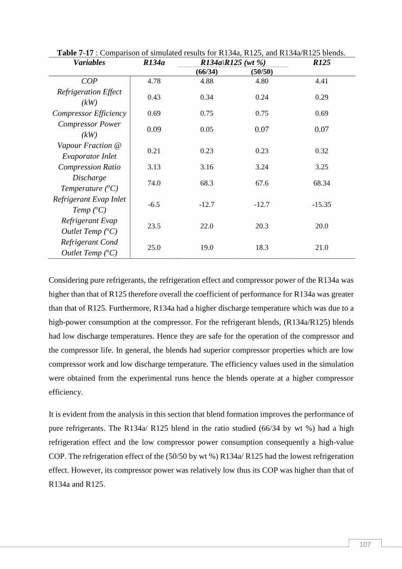
107
Table 7-17 : Comparison of simulated results for R134a, R125, and R134a/R125 blends.
Variables R134a R134a\R125 (wt %) R125 (66/34) (50/50)
COP 4.78 4.88 4.80 4.41
Refrigeration Effect
(kW) 0.43 0.34 0.24 0.29
Compressor Efficiency 0.69 0.75 0.75 0.69
Compressor Power
(kW) 0.09 0.05 0.07 0.07
Vapour Fraction @
Evaporator Inlet 0.21 0.23 0.23 0.32
Compression Ratio 3.13 3.16 3.24 3.25
Discharge
Temperature (oC) 74.0 68.3 67.6 68.34
Refrigerant Evap Inlet
Temp (oC) -6.5 -12.7 -12.7 -15.35
Refrigerant Evap
Outlet Temp (oC) 23.5 22.0 20.3 20.0
Refrigerant Cond
Outlet Temp (oC) 25.0 19.0 18.3 21.0
Considering pure refrigerants, the refrigeration effect and compressor power of the R134a was
higher than that of R125 therefore overall the coefficient of performance for R134a was greater
than that of R125. Furthermore, R134a had a higher discharge temperature which was due to a
high-power consumption at the compressor. For the refrigerant blends, (R134a/R125) blends
had low discharge temperatures. Hence they are safe for the operation of the compressor and
the compressor life. In general, the blends had superior compressor properties which are low
compressor work and low discharge temperature. The efficiency values used in the simulation
were obtained from the experimental runs hence the blends operate at a higher compressor
efficiency.
It is evident from the analysis in this section that blend formation improves the performance of
pure refrigerants. The R134a/ R125 blend in the ratio studied (66/34 by wt %) had a high
refrigeration effect and the low compressor power consumption consequently a high-value
COP. The refrigeration effect of the (50/50 by wt %) R134a/ R125 had the lowest refrigeration
effect. However, its compressor power was relatively low thus its COP was higher than that of
R134a and R125.

108
Refrigerant R134a expanded most favorable at the expansion valve as it existed with the largest
percentage of the liquid phase in the two-phase mixture whereas R125 had the lowest
proportion of liquid. However, R125 gave the lowest temperature at the evaporator inlet than
R134a thus it is an excellent low-temperature refrigerant.
From the analysis carried out above, the R134a/R125 (66/34 by wt %) blend is the best
performing blend in the refrigerant unit operating conditions investigated in this study and can
be utilised in medium temperature applications.

109
Chapter 8
8 Conclusions
The main objective of this study was to commission a refrigerant test rig and investigate the
performance of various refrigerant blends. The apparatus was successfully commissioned using
refrigerant R134a.
The operating range of the refrigeration unit is within -20 to 100 oC, sealing under vacuum
pressures of 26.6 kPa at room temperature and a maximum pressure limit of 1.9 MPa.
Results from the trial runs carried out with refrigerant R134a indicate that the equipment could
produce accurate and reliable refrigeration effect, therefore, deeming it to be suitable for
refrigeration studies.
The commercial refrigerant blends studied in the project included R413a and R507 whereas
the blend synthesised in this study were R134a/R125 (66/34 by wt %) and R134a/R125 (50/50
by wt %). In comparing the performance of commercial refrigerant blends, refrigerant blend
R507a performed better than refrigerant R413a in both the experimental and simulation
analyses. The COP values for R507a and R143a in the experimental studies were 4.54 and 3.57
respectively, whereas in the simulation the COP values were 5.00 and 4.00 respectively.
However, the performance of refrigerant R413a is comparable to that of refrigerant R134a,
used as the reference refrigerant in this study. For this reason, refrigerant blend R413a is a
potential candidate to be applied as a replacement of refrigerant R134a.
The results from the simulations performed using Aspen Plus® V8.6 utilising REFPROP
method to evaluate the performance of the refrigerants. The generated COP results deviated
from the experimental data for the refrigerants R134a, R413a and R507a as per the following
percentage differences, 2.89%, 9.64% and 11.36% respectively. Thus, it can be concluded that
the unit performance is close to the simulation (ideal) based on the COP values which are the
overall performance measurement of a refrigerant.
Considering the blends synthesised for this study, refrigerant blend R134a/R125 (66/34 by wt
%) displayed better performance than R134a/R125 (50/50 by wt %). The former had a COP
value of 4.88, refrigeration effect of 0.34 kW and compressor power of 0.05 kW whereas the
latter had COP value of 4.80, refrigeration effect of 0.24 kW and compressor power of 0.07
kW. This outcome is favorable since R134a, with a lower GWP, constitutes a larger percentage

110
in the blend. Thus, the R134a/R125 (66/34 by wt %) blend has a minimal environmental impact
compared to the R134a/R125 (50/50 by wt %) blend. Moreover, the synthesised R134a/R125
blends displayed better performance than the pure refrigerants (R134a, COP value of 4.78 and
R125, COP value of 4.41) in the comparative analysis of the simulation results.
Overall, of all the refrigerants investigated in this study R507A (R134A/R143a, 50/50 wt %) a
commercial blend and R134a/R125 (66/34 by wt %) a laboratory synthesised blend were the
better performing refrigerants from those investigated. The refrigeration effect for R507 was
0.4 kW whereas for R134a/R125 (66/34 by wt %) was 0.34 kW. However, the compression
work of R507a was 0.08 kW which is higher than that of R134a/R125 (66/34 by wt %) which
was 0.07 kW. The COP values for R507a a commercial blend and R134a/R125 (66/34 by wt
%) the synthesised blend were 5.00 and 4.88 respectively. Incorporating the environmental
factors R134a/R125 (66/34 by wt %) with GWP value of just above 1300 had an overall more
desirable performance than R507 with a GWP value of 3900.

111
Chapter 9
9 Recommendations
To improve the performance and versatility of the refrigerant unit and obtain accurate data it is
imperative to carry out the following modifications in the unit:
1. The distance between the expansion valve and the evaporator inlet should be reduced
because it lowers the refrigerating capacity of the refrigerant in the evaporator as there
is extra heat load along the pipeline.
2. The water valve at the evaporator water bath needs to be replaced with a smaller
flowmeter graduated in the range 0.1 -1 litre.
3. Improvement in the method of cooling the water in the condenser water bath, so as to
keep the condenser temperature constant, thus maintain a steady temperature in the unit
for prolonged periods.
4. Installation of a pressure sensor at the expansion valve to report the conditions
accurately at the expansion valve.
5. The configuration at the T-junction at the SA-01 inlet should be changed as it is
suspected to be the cause of a large refrigerant loss at high operating pressures.
6. The operation of other cycles (Two stage Vapour–Compression Cycle, Cascade
System, and Vapour –Compression Cycle with a Suction-line Heat Exchange) so as to
utilise the equipment to the maximum of its design capabilities.
112
References
Abdelaziz, O., Fricke, B. and Vineyard, E. A. 2012. Development of Low Global Warming
Potential Refrigerant Solutions for Commercial Refrigeration Systems using a Life
Cycle Climate Performance Design Tool. International Refrigeration and Air
Conditioning Conference Purdue: Oak Ridge National Laboratory, Energy and
Transportation Science Division, Oak Ridge, TN, USA.
Ahamed, J., Saidur, R. and Masjuki, H. 2011. A review on exergy analysis of vapor
compression refrigeration system. Renewable and Sustainable Energy Reviews, 15,
1593-1600.
Air-Conditioning Heating and Refrigeration Institute, A. 2007. 2007 Performance Rating of
Commercial and Industry Unitary Air-Conditioning and Heat Pump Equipment.
ANSI/AHRI Standard 340/360-2007 with Addenda 1and 2. Wilson Boulevard, Suite
500 ARLINGTON ,USA: Air-Conditioning Heating and Refrigeration Institute.
Akintunde, M. 2013. Experimental Study of R134a, R406A and R600a Blends as Alternative
To Freon 12. IOSR Journal of Mechanical and Civil Engineering, 7, 40-46.
Angell, J. 1988. An update through 1985 of the variations in global total ozone and north
temperate layer-mean ozone. Journal of Applied Meteorology, 27, 91-97.
Arora, A. and Kaushik, S. 2008. Theoretical analysis of a vapour compression refrigeration
system with R502, R404A and R507A. International Journal of Refrigeration, 31,
998-1005.
Arora, C. P. 2009. Refrigeration and Air Conditioning, New Dehli, Tata McGraw-Hill
Companies.
Baskaran, A. and Mathews, P. K. 2012. A Performance comparison of vapour compression
refrigeration system using Eco friendly refrigerants of low global warming potential.
International journal of scientific and research publications, 2, 1-8.
Baxter, V., Fischer, S. and Sand, J. R. 1998. Global warming implications of replacing
ozone-depleting refrigerants. ASHRAE journal, 40, 23.
Bhatkar, V. W., Kriplani, V. and Awari, G. 2013. Alternative refrigerants in vapour
compression refrigeration cycle for sustainable environment: a review of recent
research. International Journal of Environmental Science and Technology, 10, 871-
880.
Bitzter 2014. Refrigerant Report 18. 17th ed. www.bitzer.de/shared_media/documentation/a-
501-18.pdf [29 Feb 2016].
Bolaji, B. O. 2011. Performance investigation of ozone-friendly R404A and R507
refrigerants as alternatives to R22 in a window air-conditioner. Energy and Buildings,
43, 3139-3143.
Breidenich, C., Magraw, D., Rowley, A. and Rubin, J. W. 1998. The Kyoto protocol to the
United Nations framework convention on climate change. The American Journal of
International Law, 92, 315-331.

113
Brijendra, K. Y., Suresh, K. B. and Rohit, C. 2017. Replacement of R22 in Vapour
Compression Refrigeration Cycle with Mixture of Environment Friendly Refrigerant -
did not match any articles. International Journal of Engineering Technology and
Applied Science, Vol. 3.
Calm, J. M. 2008. The next generation of refrigerants–Historical review, considerations, and
outlook. International Journal of Refrigeration, 31, 1123-1133.
Çengel, Y. A. and Boles, M. A. 2006. Thermodynamics: An Engineering Approach,
McGraw-Hill, New York.
Chesi, A., Ferrara, G., Ferrari, L. and Tarani, F. 2012. Setup and characterisation of a multi-
purpose test rig for R744 refrigerating cycles and equipment. International Journal of
Refrigeration, 35, 1848-1859.
Coggins, C. L. 2007. Single-and multiple-stage cascaded vapor compression refrigeration for
electronics cooling. Georgia Institute of Technology.
Dalkilic, A. and Wongwises, S. 2010. A performance comparison of vapour-compression
refrigeration system using various alternative refrigerants. International
Communications in Heat and Mass Transfer, 37, 1340-1349.
Datta, S. P., Das, P. K. and Mukhopadhyay, S. Effect of refrigerant charge, compressor speed
and air flow through the evaporator on the performance of an automotive air
conditioning system. 15th International Refrigeration and Air Conditioning
Conference July 14-17, 2014 2014 Purdue.
Dennis, L. O. N., William, J. M., Roberto, R. A., Daniel, J. D. and Cecily, M. G. 2010.
ASHRA Handbook of Refrigeration, 1791 Tullie Circle, N.E., Atlanta, GA 30329,
American Society of Heating, Refrigerating and Air-Conditioning Engineers, Inc.
Domanski, P. A. Comparable performance evaluation of HC and HFC refrigerants in an
optimized system. 7th IIR Gustav Lorentzen Conference on Natural Working Fluids
May 28-31, 2006 Trondheim, Norway.
Donald, M. E., Harold, G. L., Ramon, P. and Brian, C. K. 1997. ASHRA Handbook of
Refrigeration, 1791 Tullie Circle, N.E., Atlanta, GA 30329, American Society of
Heating, Refrigerating and Air-Conditioning Engineers, Inc.
Elsayed, A. O. and Hariri, A. S. Effect of condenser air flow on the performance of split air
conditioner. World Renewable Energy Congress-Sweden; , 8-13 May; 2011; 2011
Linköping; Sweden. Linköping University Electronic Press, 2134-2141.
Ely, J. F. and Huber, M. L. 1990. A predictive extended corresponding states model for pure
and mixed refrigerants.
Emerson 1969. Refrigeration Manual Part-4 System Design. In: PRODUCTS, C. B. (ed.)
Emerson Climate Technology.
Emerson Climate Technologies Ae4-1299 R9 2010. Application Guidelines for K4
Refrigeration Copeland Scroll® Compressors 2 - 6 Horsepower. In: PRODUCTS, C.
B. (ed.). Printed in the U.S.A.

114
Goetzler, W., Sutherland, T., Rassi, M. and Burgos, J. 2014. Research & development
roadmap for next-generation low global warming potential refrigerants. In: ENERGY
(ed.) Energy Efficiency and Renewable Energy. Washington, DC: U.S.A: Navigant
Consulting, Inc.
Gomaa, A. 2015. Performance Characteristics of Automotive Air Conditioning System with
Refrigerant R134a and Its Alternatives. International Journal of Energy and Power
Engineering.
Gupta, M., Aftab Anjum*, Ansari, N. A. and Rs, M. 2017. Performance Analysis of a Two
Stage Vapour Compression Refrigeration System Utilizing the Waste Heat of the
Intercooler for Water Heating. Journal of Fundamentals of Renewable Energy and
Applications, 7.
Halimic, E., Ross, D., Agnew, B., Anderson, A. and Potts, I. 2003. A comparison of the
operating performance of alternative refrigerants. Applied Thermal Engineering, 23,
1441-1451.
Heldon 2009a. Suction Accumulators. www.henrytech.com.au [24 Mar 2016].
Heldon 2009b. Vibrator Eliminators. www.heldon.com.au [23 Mar 2016].
Hesselgreaves, J. E. 2011. Compact Heat Exchangers Selection , Design and operation,
Lockport, NY, USA, Elsevier Science & Technology Books.
Hoşöz, M. 2005. Performance comparison of single-stage and cascade refrigeration systems
using R134a as the working fluid. Turkish Journal of Engineering and Environmental
Sciences, 29, 285-296.
Huber, M. L., Friend, D. G. and James F. Ely 1992. Prediction of the Thermal Conductivity
of Refrigerants and Refrigerant Mixtures. Fluid Phase Equilibria, 80:249-261.
Hundy, G. F., Trott, A. R. and Welch, T. 2008. Refrigeration and Air-conditioning,
Butterworth-Heinemann.
Hwang, Y., Jin, D.-H. and Radermacher, R. 2004. Comparison of hydrocarbon R-290 and
two HFC blends R-404A and R-410A for medium temperature refrigeration
applications. Final Interim Report to ARI, Global Refrigerant Environmental
Evaluation Network (GREEN) Program, CEEE Department of Engineering,
University of Maryland, USA.
Hwang, Y., Jin, D.-H. and Radermacher, R. 2007. Comparison of R-290 and two HFC blends
for walk-in refrigeration systems. International Journal of Refrigeration, 30, 633-641.
Isceon Refrigerants 1998. R413A (ISCEON 49) Drop-In Replacement for R12, ODP Zero
Compatible with traditional lubricants. In: RHODIA LIMITED, I. H. (ed.) Bristol
BS11 9YF England. www.kemikaal.ee/lie/failid/brochure49.pdf [19 Apr 2017].
Jain, V., Kachhwaha, S. S. and Mishra, R. S. 2011. Comparative performance study of
vapour compression refrigeration system with R22/R134a/R410A/R407C/M20.
International Journal of Energy and Environment, 55, 297-310.
115
Jeong, J. H., Park, S.-G., Sarker, D. and Chang, K. S. 2012. Numerical simulation of the
effects of a suction line heat exchanger on vapor compression refrigeration cycle
performance. Journal of Mechanical Science and Technology, 26, 1213.
Jerald, L. A. and Kumaran, D. S. 2014. Investigations on the performance of vapour
compression system retrofitted with zeotropic refrigerant R404a. American Journal of
Environmental Sciences, 10, 35.
Jung, D., Kim, C.-B., Hwang, S.-M. and Kim, K.-K. 2003. Condensation heat transfer
coefficients of R22, R407C, and R410A on a horizontal plain, low fin, and turbo-C
tubes. International Journal of Refrigeration, 26, 485-491.
Jung, D., Song, Y. and Park, B. 2000. Performance des mélanges de frigorigènes utilisés pour
remplacer le HCFC22. International Journal of Refrigeration, 23, 466-474.
Kakac, S., Liu, H. and Pramuanjaroenkij, A. 2012. Heat exchangers: Selection, Rating, and
Thermal design, Boca Raton, Florida, CRC press.
Karagoz, S., Yilmaz, M., Comakli, O. and Ozyurt, O. 2004. R134a and various mixtures of
R22/R134a as an alternative to R22 in vapour compression heat pumps. Energy
conversion and management, 45, 181-196.
Kim, J. H., Cho, J. M., Lee, I. H., Lee, J. S. and Kim, M. S. 2007. Circulation concentration
of CO 2/propane mixtures and the effect of their charge on the cooling performance in
an air-conditioning system. International Journal of Refrigeration, 30, 43-49.
Kim, M. and Didion, D. 1995. Simulation of isothermal and adiabatic leak processes of
zeotropic refrigerant mixtures. HVAC&R Research, 1, 3-20.
Klein, S., Reindl, D. and Brownell, K. 2000. Refrigeration system performance using liquid-
suction heat exchangers. International Journal of Refrigeration, 23, 588-596.
Kumar, S. S., Sivaram, A. and Rajavel, R. 2015. Thermodynamic Analysis of a Cascade
Refrigeration System with R744/R290 Mixtures. Indian Journal of Science and
Technology, 8.
Lavelle, J. 2006. Understanding Refrigerant Blend Performance Part 1. In: INC, N. R. (ed.).
Mani, K. and Selladurai, V. 2008. Experimental analysis of a new refrigerant mixture as
drop-in replacement for CFC12 and HFC134a. International Journal of Thermal
Sciences, 47, 1490-1495.
Mani, K., Selladurai, V. and Murugan, N. 2013. Development of Mathematical Models for
Predicting Performance of CFC12, HFC134a and R290/R600 Mixture Refrigerants
using Design of Experiments. International Journal of Thermodynamics, 16, 43-53.
Mcgeorge, H. D. 1998. Marine auxiliary machinery, Linacre House, Jordan Hill, Oxford 0X2
BDP, Butterworth-Heinemann.
Mclinden, M. O., Klein, S. A. and Perkins, R. A. 2000. An extended corresponding states
model for the thermal conductivity of refrigerants and refrigerant mixtures.
International Journal of Refrigeration, 23, 43-63.

116
Mishra, R. 2014. Thermodynamic Performance Evaluation of Multi-Evaporators Single
Compressor and Single Expansion Valve and Liquid Vapour Heat Exchanger in
Vapour Compression Refrigeration Systems using Thirteen Ecofriendly Refrigerants
for Reducing Global Warming and Ozone depletion. International Journal, 2, 325-
332.
Moffat, R. J. 1988. Describing the uncertainties in experimental results. Experimental
Thermal and Fluid Science, 1, 3-17.
Mohanraj, M., Muraleedharan, C. and Jayaraj, S. 2011. A review on recent developments in
new refrigerant mixtures for vapour compression‐based refrigeration, air‐conditioning
and heat pump units. International Journal of Energy Research, 35, 647-669.
Molina, M. J. and Rowland, F. S. 1974. Stratospheric sink for chlorofluoromethanes: chlorine
atom-catalysed destruction of ozone. Nature, 249, 810-812.
Moran, M. J. and Shapiro, H. N. 2006. Fundamentals of Engineering Thermodynamics, West
Sussex, England, John Wiley & Sons Ltd, .
Mulroy, W., Domanski, P. and Didion, D. 1994a. Glide matching with binary and ternary
zeotropic refrigerant mixtures Part 2. A computer simulation. International Journal of
Refrigeration, 17, 226-230.
Mulroy, W., Domanski, P. A. and Didion, D. 1994b. Glide matching with binary and ternary
zeotropic refrigerant mixtures Part 1. An experimental study. International Journal of
Refrigeration, 17, 220-225.
Narayan, L., Arya, A. and Khare, S. 2013. A comparative study for retrofitting of R-12
vapour compression refrigeration system by eco-friendly refrigerants R-134a, R-413a,
R-423a. International Journal of Application of Engineering and Technology, 2.
Outcalt, S. L. and Mclinden, M. O. 1996. A Modified Benedict–Webb–Rubin Equation of
State for the Thermodynamic Properties of R152a (1, 1‐difluoroethane). Journal of
Physical and Chemical Reference Data, 25, 605-636.
Padilla, M., Revellin, R. and Bonjour, J. 2010. Exergy analysis of R413A as replacement of
R12 in a domestic refrigeration system. Energy Conversion and Management, 51,
2195-2201.
Park, K.-J., Shim, Y.-B. and Jung, D. 2009. A ‘drop-in’refrigerant R431A for replacing
HCFC22 in residential air-conditioners and heat pumps. Energy Conversion and
Management, 50, 1671-1675.
Parker Hannifin Corporation 2015. Combination Moisture & Liquid Indicators for
Refrigerants R134a, R22, R404A, R407C, R407F, R410A or R507. In: EUROPE, I.
G. R. A. A. C. (ed.). Cortonwood Drive, Brampton Barnsley S73 OUF - United
Kingdom.
Pelchem 2014. Pelchem SOC Ltd Overview. In: PELCHEM (ed.) Fluorochemical
excellence.

117
Prapainop, R. and Suen, K. 2012. Effects of refrigerant properties on refrigerant performance
comparison: A review. International Journal of Engineering and Research and
Applications (IJERA), 2, 486-493.
Rajapaksha, L. 2007. Influence of special attributes of zeotropic refrigerant mixtures on
design and operation of vapour compression refrigeration and heat pump systems.
Energy Conversion and Management, 48, 539-545.
Rasti, M., Hatamipour, M. S., Aghamiri, S. F. and Tavakoli, M. 2011. Experimental study of
R600a and R436a to replace R134a in a domestic refrigerator and freezer. 7th
International Chemical Engineering Congress & Exhibition. Kish, Iran.
Rigola, J., Escanes, F., Oliva, A. and Pérez-Segarra, C. 1996. Numerical study of a single
stage vapor compression refrigerant unit using non-contaminant refrigerants.
Rigola, J., Pérez-Segarra, C., Garcia-Valladares, O., Serra, J., Escriba, M. and Pons, J. 1998.
Numerical study and experimental validation of a complete vapor compression
refrigerating cycle.
Sami, S. M. and Desjardins, D. E. 2000. Performance comparative study of new alternatives
to R‐502 inside air/refrigerant enhanced surface tubing. International Journal of
Energy Research, 24, 177-186.
Sapali, S. 2009. Refrigeration and Air conditioning, PHI Learning Pvt. Ltd.
Satola, B. J. 2014. Molecular Targeting of Refrigerant Mixtures,. University of KwaZulu-
Natal, School of Engineering, Howard College Campus, For the degree Doctor of
Philosophy in Engineering (Chemical Engineering).
.
Satyanarayana, M. D. V. and Kotaiah, B. 2012. Impact of CFCs on Ozone layer and Global
warming. IOSR Journal of Engineering (IOSRJEN), Vol. 2 059-069.
Sekiya, A. and Misaki, S. 2000. The potential of hydrofluoroethers to replace CFCs, HCFCs
and PFCs. Journal of Fluorine Chemistry, 101, 215-221.
Sivasakthivel, T. and Reddy, K. S. K. 2011. Ozone layer depletion and its effects: a review.
International Journal of Environmental Science and Development, 2, 30.
Smith, J. M., Ness, H. C. V. and Abbott, M. M. 2005. Introduction to Chemical Engineering
Thermodynamics, Boston, McGraw-Hill Higher Education.
South African Government Press Release. 2009. Fluorochemical Expansion Initiative launch
[Online]. http://www.gov.za/m-mangena-fluorochemical-expansion-initiative-launch.
[Accessed 17 May 2017].
Stanciu, C., Gheorghian, A., Stanciu, D. and Dobrovicescu, A. 2011. Exergy analysis and
refrigerant effect on The operation and performance limits of a One stage vapor
compression Refrigeration system. Termotehnica, 1, 36-42.
118
Swagelok Company 2013. Swagelok Metering Valves MS-01-142. Kalrez—TM DuPont.
USA: www.swagelok.com [Accessed 02 Apr 2016].
Szymurski, S. R. 2005. Refrigerant Blends, 9th Annual Financial Agent Workshop the World
bank. In: INSTITUTE, A.-C. R. (ed.) Air-Conditioning & Refrigeration Institute.
Taylor, B. N. and Kuyatt, C. E. 1994. Guidelines for evaluating and expressing the
uncertainty of NIST measurement results, US Department of Commerce, Technology
Administration, National Institute of Standards and Technology Gaithersburg, MD.
Tillner-Roth, R. and Baehr, H. D. 1994. An international standard formulation for the
thermodynamic properties of 1, 1, 1, 2‐Tetrafluoroethane (HFC‐134a) for
temperatures from 170 K to 455 K and pressures up to 70 MPa. Journal of Physical
and Chemical Reference Data, 23, 657-729.
Tuta, E. C. and Orozco, M. R. Computational tool for simulation of power and refrigeration
cycles. IOP Conference Series: Materials Science and Engineering, 2016. IOP
Publishing, 012017.
United Nations Epa 2014. Benefits of Addressing HFCs under the Montreal Protocol.
Stratospheric Protection Divivsion Office of Atmospheric Programs Office of Air and
Radiation.
United Nations Montreal Protocol. 1 January 1989. Montreal Protocol on Substances that
Deplete the Ozone Layer. Montreal Protocol, 1987 Montreal, Canada.
United States Epa 2007. Achievements in Stratospheric Ozone Protection Progress Report.
In: AGENCY, U. S. E. P. (ed.) Office of Air and Radiation. Washington,DC 20460.
Venkatarathnam, G. and Murthy, S. S. 2012. Refrigerants for vapour compression
refrigeration systems. Resonance, 17, 139-162.
Wagner, W. and Pruß, A. 2002. The IAPWS formulation 1995 for the thermodynamic
properties of ordinary water substance for general and scientific use. Journal of
Physical and Chemical Reference Data, 31, 387-535.
Whitman, B., Johnson, B., Tomczyk, J. and Silberstein, E. 2013. Refrigeration and Air
Conditioning Technology, Clifton Park ,USA, Delmar Cengage Learning.
Wongwises, S., Kamboon, A. and Orachon, B. 2006. Experimental investigation of
hydrocarbon mixtures to replace HFC-134a in an automotive air conditioning system.
Energy Conversion and Management, 47, 1644-1659.
Yadav, R. 2007. Thermodynamics and Heat Engines Central Publishing House.
Yataganbaba, A., Kilicarslan, A. and Kurtbaş, İ. 2015. Exergy analysis of R1234yf and
R1234ze as R134a replacements in a two evaporator vapour compression refrigeration
system. International Journal of Refrigeration, 60, 26-37.
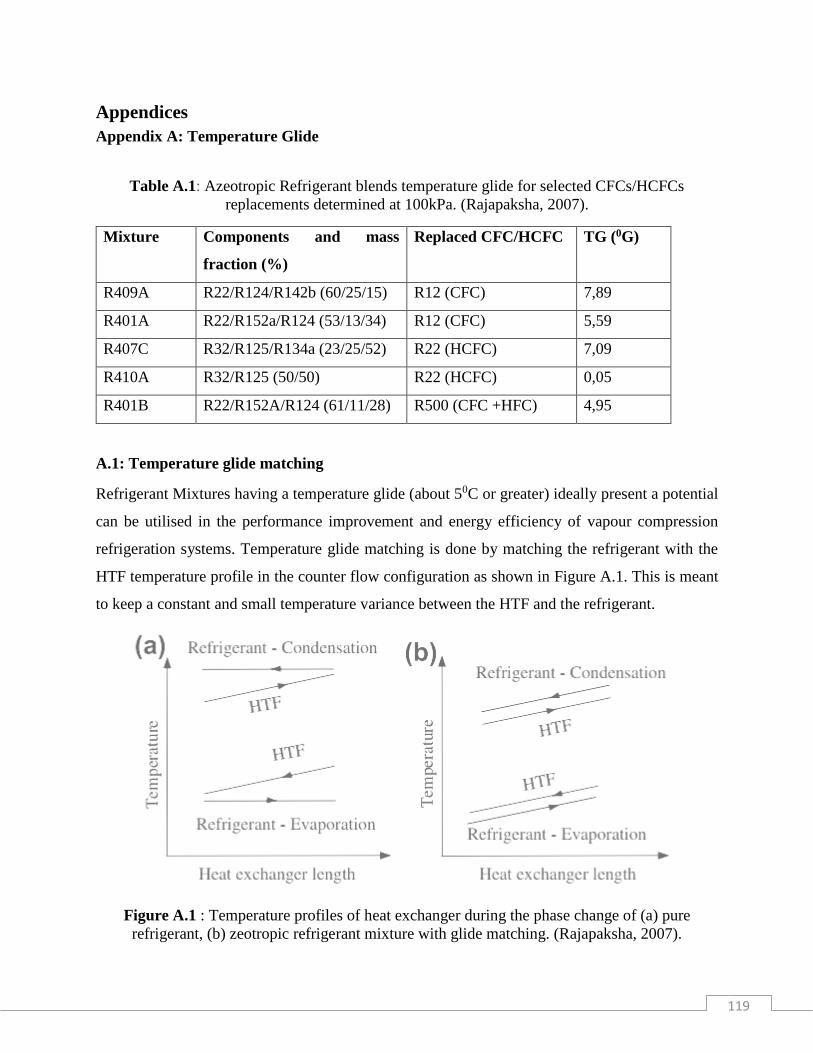
119
Appendices
Appendix A: Temperature Glide
Table A.1: Azeotropic Refrigerant blends temperature glide for selected CFCs/HCFCs
replacements determined at 100kPa. (Rajapaksha, 2007).
Mixture Components and mass
fraction (%)
Replaced CFC/HCFC TG (0G)
R409A R22/R124/R142b (60/25/15) R12 (CFC) 7,89
R401A R22/R152a/R124 (53/13/34) R12 (CFC) 5,59
R407C R32/R125/R134a (23/25/52) R22 (HCFC) 7,09
R410A R32/R125 (50/50) R22 (HCFC) 0,05
R401B R22/R152A/R124 (61/11/28) R500 (CFC +HFC) 4,95
A.1: Temperature glide matching
Refrigerant Mixtures having a temperature glide (about 50C or greater) ideally present a potential
can be utilised in the performance improvement and energy efficiency of vapour compression
refrigeration systems. Temperature glide matching is done by matching the refrigerant with the
HTF temperature profile in the counter flow configuration as shown in Figure A.1. This is meant
to keep a constant and small temperature variance between the HTF and the refrigerant.
Figure A.1 : Temperature profiles of heat exchanger during the phase change of (a) pure
refrigerant, (b) zeotropic refrigerant mixture with glide matching. (Rajapaksha, 2007).

120
Glide matching improves the efficiency of the system by reducing irreversibility of the heat
transfer process Glide matching is only achievable in heat exchangers with certain geometries
where counter-flow of fluids is possible, such as concentric tubes, shell and tube and flat heat
exchangers. Glide matching reduces the entropy generated in the heat exchanger during the phase
change thus increasing the efficiency of the system. Moreover, it improves the COP as the
compressor will be operating under reduced pressure. Atmospheric air and water/glycol mixture
and are a good example of HTFs for glide matching in the condenser and evaporator and for vapour
compression systems (Mulroy et al., 1994a; Mulroy et al., 1994b).Glide matching is best suited
for liquid-liquid systems and is affected by changes in operating pressure. Understanding glide
properties of refrigerants are essential in identifying problems in retrofitting systems and in new
refrigeration design and hardware improvements to incorporate temperature glide and composition
change so as to improve the efficiency of the system (Rajapaksha, 2007). Mixtures exhibiting a
glide of / less than 2K are termed ‘near-azeotropes’ and are often treated as a pure substance for
the purposes of design (Hundy et al., 2008).
A.2: Effects of Phase Change of Zeotropic blends on Heat Transfer Coefficients (HTC)
Due to preferential boiling or condensation, composition shifts occur within the different phases
of the fluid. Consider the condensation of a binary mixture of components A and B on a cold
surface. Component A with a higher boiling point will condense first reducing its vapour
concentration (and consequently its partial pressure) closer to the wall. This results in the formation
of a vapour diffusion film (with concentration gradient) between the condensate and bulk vapour
(Figure A.2).
This vapour diffusion film acts as an additional thermal resistance. The reduction of interfacial
temperature from Tb to Ti (and consequently reduction of the temperature driving force for
conduction in the condensate film) results in lower heat transfer coefficients when compared to an
azeotropic mixture.

121
Figure A.2 : Pressure and temperature profile for condensation of a non-azeotropic mixture.
(Jung et al., 2003).
Jung et al. (2003) investigated the heat transfer coefficients for condensation of R22, R407C, and
R410A on different tube surfaces. The HTC’s of zeotropic R407C were up to 50 % lower than
those of R22. This was attributed to the presence of the diffusion vapour film.
Appendix B: Technical Information of the Equipment Components
The technical specifications for the suction accumulator, compressor and the valves are stated
below:
B.1: Suction Accumulators
Manufactured in accordance with AS 2971, AS1210 and UL207.
General Safe Working Pressure for Heldon Suction Accumulators is 2.500 kPa.
General minimum burst Pressure for Heldon Accumulators is 12500 kPa.
Design temperature range of all Heldon Accumulators is -30 0C to +50 0C.
Copper tubing and fittings in accordance with AS 1571-1995 or ASTM B28.

122
Table B.1 : Compressor Specifications
Type Reciprocating
Model Bitzer 2KES-05(Y)
No. cylinder x bore x stroke 2 x 30 mm x 33 mm
Cooling Air
Refrigerant HFC (spec. R134a, R404A, R407A/C/F,
R507A
Oil type POE (Emkarate 32)
Oil charge 1.00 dm3
Maximum pressure (LP/HP) 1.9/2.8 MPa
Displacement at 50Hz (1450 RPM) 4.06 m3/hr
Displacement at 60Hz (1750 RPM) 4.90 m3/hr
Motor 230/400 V-3-50 Hz
Drive 3 phase motor
Capacity adjustment Variable frequency drive (30 -70 Hz)
Maximum operating current 2.8 A(Y)
Maximum power consumption 1.5 kW
Table B.2 : Valves Specifications (Swagelok Company, 2013). Expansion Valves Metering Valves
Code on the Unit SS-4L-BU-MH SS-4MG-BU-MH
Description Metering Valve Buna O-rings ,
MH Handle
Metering Valve L-SERIES,
Buna O-rings, MH
Orifice 0.128 inch/3.25 mm 0.0056 inch/1.42 mm
Working Pressure/bars 68.9 68.9
Temperature/0C -23 to 148 -23 to 148
Cv 0.004 to 0.16 0.004 to 0.16
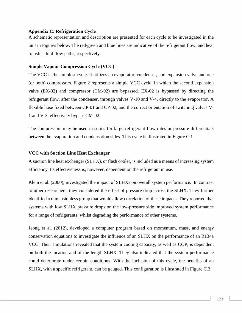
123
Appendix C: Refrigeration Cycle
A schematic representation and description are presented for each cycle to be investigated in the
unit in Figures below. The red/green and blue lines are indicative of the refrigerant flow, and heat
transfer fluid flow paths, respectively.
Simple Vapour Compression Cycle (VCC)
The VCC is the simplest cycle. It utilizes an evaporator, condenser, and expansion valve and one
(or both) compressors. Figure 2 represents a simple VCC cycle, in which the second expansion
valve (EX-02) and compressor (CM-02) are bypassed. EX-02 is bypassed by directing the
refrigerant flow, after the condenser, through valves V-10 and V-4, directly to the evaporator. A
flexible hose fixed between CP-01 and CP-02, and the correct orientation of switching valves V-
1 and V-2, effectively bypass CM-02.
The compressors may be used in series for large refrigerant flow rates or pressure differentials
between the evaporation and condensation sides. This cycle is illustrated in Figure C.1.
VCC with Suction Line Heat Exchanger
A suction line heat exchanger (SLHX), or flash cooler, is included as a means of increasing system
efficiency. Its effectiveness is, however, dependent on the refrigerant in use.
Klein et al. (2000), investigated the impact of SLHXs on overall system performance. In contrast
to other researchers, they considered the effect of pressure drop across the SLHX. They further
identified a dimensionless group that would allow correlation of these impacts. They reported that
systems with low SLHX pressure drops on the low-pressure side improved system performance
for a range of refrigerants, whilst degrading the performance of other systems.
Jeong et al. (2012), developed a computer program based on momentum, mass, and energy
conservation equations to investigate the influence of an SLHX on the performance of an R134a
VCC. Their simulations revealed that the system cooling capacity, as well as COP, is dependent
on both the location and of the length SLHX. They also indicated that the system performance
could deteriorate under certain conditions. With the inclusion of this cycle, the benefits of an
SLHX, with a specific refrigerant, can be gauged. This configuration is illustrated in Figure C.3.

124
Cascade Refrigeration Cycle
The cascade VCC is represented in Figure C.4, where the green and red lines indicate the respective
refrigerant flows through the two cycles of the cascade system. By facilitating both these cycles
on a single unit, a direct comparison can be made for refrigerants and operating conditions.
Hoşöz (2005), conducted an experimental comparison of R134a single stage and cascade VCCs.
He found that, for a given refrigerating capacity, the cascade system exhibited lower evaporating
temperatures. The required compressor power and refrigerant flowrates were also reduced, as
compared to the single stage. Although this implies a higher COP for the lower temperature cycle,
the overall system COP is lower, due to the additional power requirement of the second
compressor. The cascade VCC leads to lower operating pressure ratios for the compressor, higher
volumetric efficiencies, and lower discharge temperatures that should lengthen compressor life.
(Kumar et al., 2015).
Multistage Refrigeration Cycle
A two-stage VCC is illustrated in Figure C.5. Splitting the condensate stream is accomplished by
two Swagelok fine metering valves (EX-01 and MV-2). The valves are equipped with Vernier
handles to allow reproducibility as well as fine control. Manipulating this will allow identification
of the optimal split ratio for a specific refrigerant.

125
VLT
1
VLT
2COMPRESSOR 2
CONTROL
PANEL
COMPRESSOR 1
CONTROL
PANEL
CN-01
HX-01
EV-01
V-5
V-10
V-1
V-4
EX-02EX-01
SG-01
CP-01
CP-03
T2
T1
T6
SA-01 SA-02
OS-02
V-6
V-2
V-12
MI-01
LR-01
MI-02
LR-02
MV-2
V-3
V-8
CH-02
CH-03
CH-04
CH-01
CP-02
V-11
V-13V-9
CV-03
CV-04
CV-01
P0
P2
P6
T0P4
CV-02
T10 P3
T4 P9
T7 P1
P5
DR-01
V-7
DR-02
T8 P7
WATER
BATH
EG/ WATER
BATHT3
OS-01
T9
CM-02CM-01
T5
CRio
LP-01
LP-02
RT-01 RT-02
FH-01
Figure C.1 : Simple VC configuration.

126
VLT
1
VLT
2COMPRESSOR 2
CONTROL
PANEL
COMPRESSOR 1
CONTROL
PANEL
CN-01
HX-01
EV-01
V-5
V-10
V-1
V-4
EX-02EX-01
SG-01
CP-01
CP-03
T2
T1
T6
SA-01 SA-02
OS-02
V-6
V-2
V-12
MI-01
LR-01
MI-02
LR-02
MV-2
V-3
V-8
CH-02
CH-03
CH-04
CH-01
CP-02
V-11
V-13V-9
CV-03
CV-04
CV-01
P0
P2
P6
T0P4
CV-02
T10 P3
T4 P9
T7 P1
P5
DR-01
V-7
DR-02
T8 P7
WATER
BATH
EG/ WATER
BATHT3
OS-01
T9
CM-02CM-01
T5
CRio
LP-01
LP-02
RT-01 RT-02
Figure C.2 : VC configuration using two compressors.
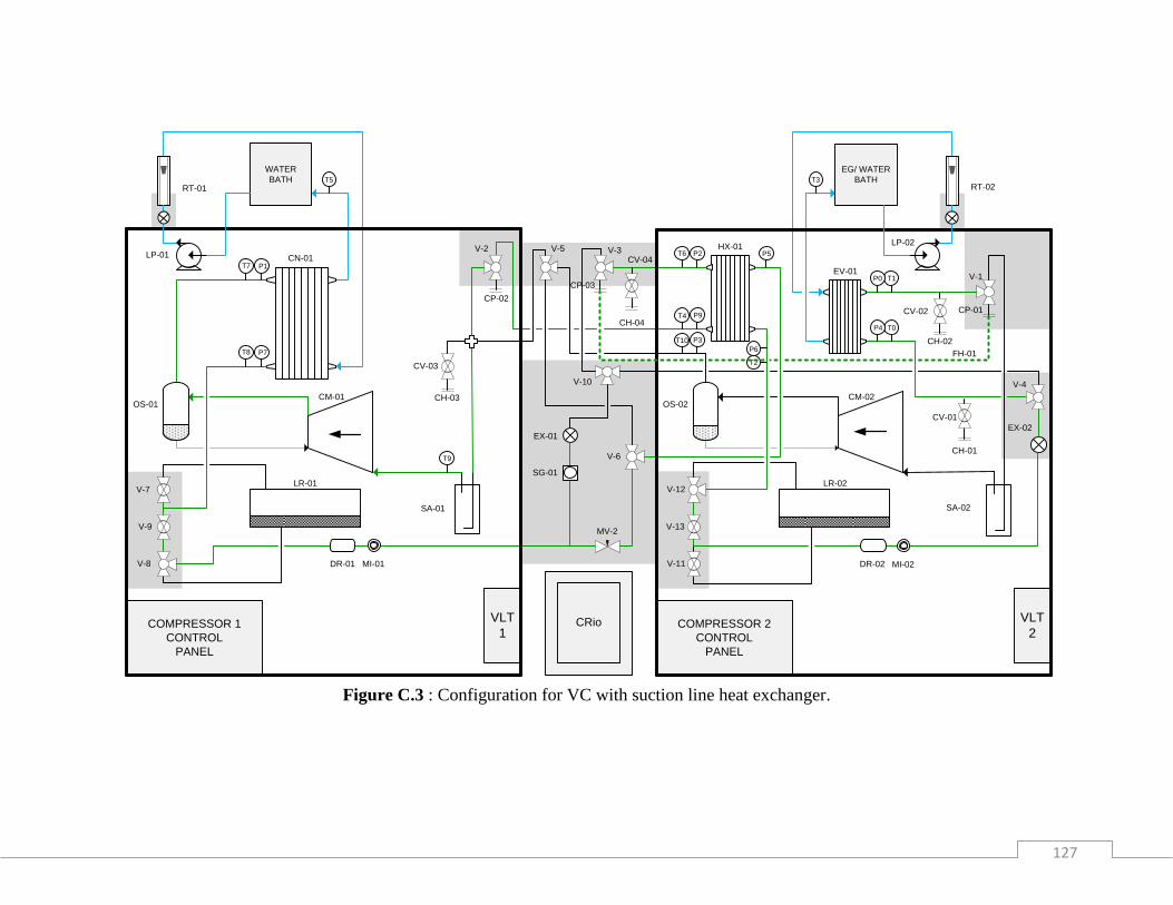
127
VLT
1
VLT
2COMPRESSOR 2
CONTROL
PANEL
COMPRESSOR 1
CONTROL
PANEL
CN-01
HX-01
EV-01
V-5
V-10
V-1
V-4
EX-02EX-01
SG-01
CP-01
CP-03
T2
T1
T6
SA-01 SA-02
OS-02
V-6
V-2
V-12
MI-01
LR-01
MI-02
LR-02
MV-2
V-3
V-8
CH-02
CH-03
CH-04
CH-01
CP-02
V-11
V-13V-9
CV-03
CV-04
CV-01
P0
P2
P6
T0P4
CV-02
T10 P3
T4 P9
T7 P1
P5
DR-01
V-7
DR-02
T8 P7
WATER
BATH
EG/ WATER
BATHT3
OS-01
T9
CM-02CM-01
T5
CRio
LP-01
LP-02
RT-01 RT-02
FH-01
Figure C.3 : Configuration for VC with suction line heat exchanger.
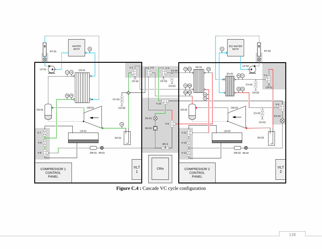
128
VLT
1
VLT
2COMPRESSOR 2
CONTROL
PANEL
COMPRESSOR 1
CONTROL
PANEL
CN-01
HX-01
EV-01
V-5
V-10
V-1
V-4
EX-02EX-01
SG-01
CP-01
CP-03
T2
T1
T6
SA-01 SA-02
OS-02
V-6
V-2
V-12
MI-01
LR-01
MI-02
LR-02
MV-2
V-3
V-8
CH-02
CH-03
CH-04
CH-01
CP-02
V-11
V-13V-9
CV-03
CV-04
CV-01
P0
P2
P6
T0P4
CV-02
T10 P3
T4 P9
T7 P1
P5
DR-01
V-7
DR-02
T8 P7
WATER
BATH
EG/ WATER
BATHT3
OS-01
T9
CM-02CM-01
T5
CRio
LP-01
LP-02
RT-01 RT-02
Figure C.4 : Cascade VC cycle configuration

129
VLT
1
VLT
2COMPRESSOR 2
CONTROL
PANEL
COMPRESSOR 1
CONTROL
PANEL
CN-01
HX-01
EV-01
V-5
V-10
V-1
V-4
EX-02EX-01
SG-01
CP-01
CP-03
T2
T1
T6
SA-01 SA-02
OS-02
V-6
V-2
V-12
MI-01
LR-01
MI-02
LR-02
MV-2
V-3
V-8
CH-02
CH-03
CH-04
CH-01
CP-02
V-11
V-13V-9
CV-03
CV-04
CV-01
P0
P2
P6
T0P4
CV-02
T10 P3
T4 P9
T7 P1
P5
DR-01
V-7
DR-02
T8 P7
WATER
BATH
EG/ WATER
BATHT3
OS-01
T9
CM-02CM-01
T5
CRio
LP-01
LP-02
RT-01 RT-02
Figure C.5 : Two-stage VC cycle configuration.
130
Appendix D: Uncertainty in Measurements
D.1: Experimental Uncertainty
There are several components which constitute to the uncertainty of a measurement, however,
these components are usually categorised in accordance with the method used to estimate their
numerical values: Type A and Type B.
An alternative nomenclature that is commonly used to classify the uncertainty in measurements
is as either the part of uncertainty from random effect or the element of uncertainty from a
systematic effect. (NIST) (Taylor and Kuyatt, 1994).
The CSU of a measurement is obtained by combining the individual standard uncertainties
Regardless of whether they are from a type A evaluation or a type B using the method of
combined standard deviations. The expanded uncertainty is the measure of certainty intended
to meet the required measurement. It is obtained by multiplying the CSU by the coverage
factor, k, to give combined expanded uncertainty represented by 𝑈(𝑥). Hence the combined
expanded uncertainty is given by:
𝑈(𝑥) = 𝑘𝑢𝑐(𝑥) D.1
where k is the coverage factor with a typical value of 2 is used to define an interval, having a
level of confidence of approximately 95 percent. (NIST) (Taylor et al 1994). This can be
expressed as:
𝑢𝑐(𝑥) = ±√∑ 𝑢𝑖
𝑖
(𝑥)2 D.2
where 𝑢𝑖(𝑥) is the standard uncertainty for a value x, such as uncertainty due to calibration
correlation or standards or uncertainty due to the instrument manufacturer and uncertainty due
to the repeatability of the measurement.

131
The combined uncertainty 𝑢𝑐(𝑥) is calculated from the uncertainty which arises from any of
the two classes of uncertainty Type A or Type B. The Type A uncertainty is calculated by
statistical methods in which the mean is taken to represent the true value. It is calculated by:
𝑢𝑖(𝑥) =𝜎
√𝑁 D.3
where 𝜎 the standard deviation of the data and N is the number of data points. Type B
uncertainty is computed by a number of methods and information related to the measurements.
The uncertainty can lie anywhere between the distribution and such distributions are known as
rectangular. They are represented by:
𝑢𝑖(𝑥) =𝑏
√3 D.4
where b is the half the width of the interval. The rectangular distribution model is always the
default model in the absence of any other information.
D.2: Temperature and Pressure Uncertainty
In refrigeration studies, temperature and pressure are the two most important parameters
measured. The combined uncertainty of temperature is given by:
𝑢𝑐(𝑇) = ±√𝑢𝑐𝑎𝑙𝑖𝑏(𝑇)2 + 𝑢𝑟𝑒𝑝(𝑇)2 + 𝑢𝑖𝑛𝑠𝑡𝑟(𝑇)2 D.5
where 𝑢𝑟𝑒𝑝(𝑇) denotes the standard uncertainty because of repeatability of a measurement
(Type A), 𝑢𝑖𝑛𝑠𝑡𝑟(𝑇) is the uncertainty of the Pt-100 standard temperature probe and 𝑢𝑐𝑎𝑙𝑖𝑏(𝑇)
denotes the standard uncertainty as a result of temperature calibration and is determined by:

132
𝑢𝑐𝑎𝑙𝑖𝑏(𝑇) = ±√𝑢𝑠𝑡𝑑(𝑇)2 + 𝑢𝑐𝑜𝑟𝑟(𝑇)2 D.6
where 𝑢𝑐𝑜𝑟𝑟(𝑇) denotes the standard uncertainty because of the temperature calibration
correlation (Type B) and 𝑢𝑠𝑡𝑑(𝑇) denotes the standard uncertainty inherent in the standard
temperature probe (Type B).
Likewise, the combined standard uncertainty in pressure is calculated by:
𝑢𝑐(𝑃) = ±√𝑢𝑐𝑜𝑟𝑟(𝑃)2 + 𝑢𝑟𝑒𝑝(𝑃)2 + 𝑢𝑠𝑡𝑑(𝑃)2 + 𝑢𝑎𝑡𝑚(𝑃)2 D.7
where 𝑢𝑐𝑜𝑟𝑟(𝑃) is the standard uncertainty due to the pressure calibration correlation (Type B),
𝑢𝑠𝑡𝑑(𝑃) is the standard uncertainty of the pressure transducer (Type B), and 𝑢𝑟𝑒𝑝(𝑃) is the
standard uncertainty due to the repeatability of the pressure measurement (Type A).
D.3: Rotameter Uncertainty
The water flowrates across the evaporator and condenser were gauged by rotameters. The
combined uncertainty of flowrate is given by:
𝑢𝑐(𝐹) = ±√𝑢𝑐𝑜𝑟𝑟(𝐹)2+𝑢𝑟𝑒𝑝(𝐹)2 D.8
where 𝑢𝑟𝑒𝑝(𝐹) is the standard uncertainty due to the repeatability of the flowrate measurement
(Type A) and 𝑢𝑐𝑜𝑟𝑟(𝑃) is the standard uncertainty due to flowrate calibration correlation (Type
B).
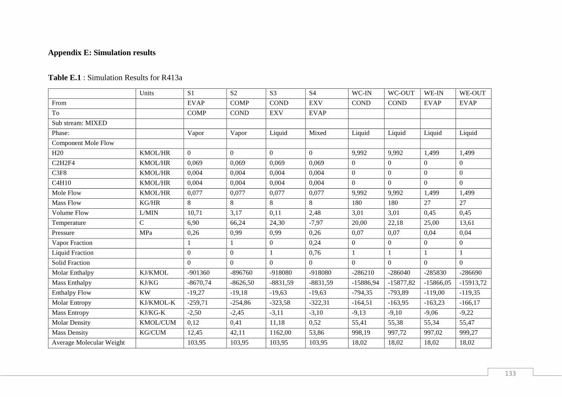
133
Appendix E: Simulation results
Table E.1 : Simulation Results for R413a
Units S1 S2 S3 S4 WC-IN WC-OUT WE-IN WE-OUT
From
EVAP COMP COND EXV COND COND EVAP EVAP
To
COMP COND EXV EVAP
Sub stream: MIXED
Phase:
Vapor Vapor Liquid Mixed Liquid Liquid Liquid Liquid
Component Mole Flow
H20 KMOL/HR 0 0 0 0 9,992 9,992 1,499 1,499
C2H2F4 KMOL/HR 0,069 0,069 0,069 0,069 0 0 0 0
C3F8 KMOL/HR 0,004 0,004 0,004 0,004 0 0 0 0
C4H10 KMOL/HR 0,004 0,004 0,004 0,004 0 0 0 0
Mole Flow KMOL/HR 0,077 0,077 0,077 0,077 9,992 9,992 1,499 1,499
Mass Flow KG/HR 8 8 8 8 180 180 27 27
Volume Flow L/MIN 10,71 3,17 0,11 2,48 3,01 3,01 0,45 0,45
Temperature C 6,90 66,24 24,30 -7,97 20,00 22,18 25,00 13,61
Pressure MPa 0,26 0,99 0,99 0,26 0,07 0,07 0,04 0,04
Vapor Fraction
1 1 0 0,24 0 0 0 0
Liquid Fraction
0 0 1 0,76 1 1 1 1
Solid Fraction
0 0 0 0 0 0 0 0
Molar Enthalpy KJ/KMOL -901360 -896760 -918080 -918080 -286210 -286040 -285830 -286690
Mass Enthalpy KJ/KG -8670,74 -8626,50 -8831,59 -8831,59 -15886,94 -15877,82 -15866,05 -15913,72
Enthalpy Flow KW -19,27 -19,18 -19,63 -19,63 -794,35 -793,89 -119,00 -119,35
Molar Entropy KJ/KMOL-K -259,71 -254,86 -323,58 -322,31 -164,51 -163,95 -163,23 -166,17
Mass Entropy KJ/KG-K -2,50 -2,45 -3,11 -3,10 -9,13 -9,10 -9,06 -9,22
Molar Density KMOL/CUM 0,12 0,41 11,18 0,52 55,41 55,38 55,34 55,47
Mass Density KG/CUM 12,45 42,11 1162,00 53,86 998,19 997,72 997,02 999,27
Average Molecular Weight
103,95 103,95 103,95 103,95 18,02 18,02 18,02 18,02
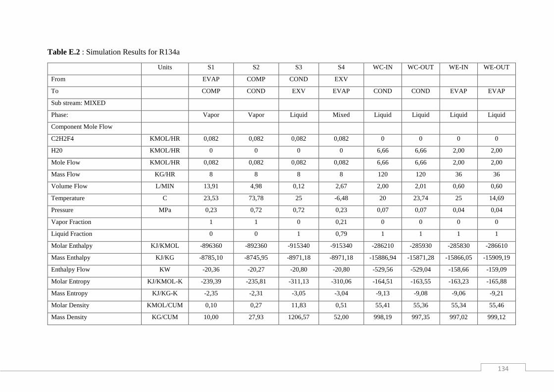
134
Table E.2 : Simulation Results for R134a
Units S1 S2 S3 S4 WC-IN WC-OUT WE-IN WE-OUT
From
EVAP COMP COND EXV
To
COMP COND EXV EVAP COND COND EVAP EVAP
Sub stream: MIXED
Phase:
Vapor Vapor Liquid Mixed Liquid Liquid Liquid Liquid
Component Mole Flow
C2H2F4 KMOL/HR 0,082 0,082 0,082 0,082 0 0 0 0
H20 KMOL/HR 0 0 0 0 6,66 6,66 2,00 2,00
Mole Flow KMOL/HR 0,082 0,082 0,082 0,082 6,66 6,66 2,00 2,00
Mass Flow KG/HR 8 8 8 8 120 120 36 36
Volume Flow L/MIN 13,91 4,98 0,12 2,67 2,00 2,01 0,60 0,60
Temperature C 23,53 73,78 25 -6,48 20 23,74 25 14,69
Pressure MPa 0,23 0,72 0,72 0,23 0,07 0,07 0,04 0,04
Vapor Fraction
1 1 0 0,21 0 0 0 0
Liquid Fraction
0 0 1 0,79 1 1 1 1
Molar Enthalpy KJ/KMOL -896360 -892360 -915340 -915340 -286210 -285930 -285830 -286610
Mass Enthalpy KJ/KG -8785,10 -8745,95 -8971,18 -8971,18 -15886,94 -15871,28 -15866,05 -15909,19
Enthalpy Flow KW -20,36 -20,27 -20,80 -20,80 -529,56 -529,04 -158,66 -159,09
Molar Entropy KJ/KMOL-K -239,39 -235,81 -311,13 -310,06 -164,51 -163,55 -163,23 -165,88
Mass Entropy KJ/KG-K -2,35 -2,31 -3,05 -3,04 -9,13 -9,08 -9,06 -9,21
Molar Density KMOL/CUM 0,10 0,27 11,83 0,51 55,41 55,36 55,34 55,46
Mass Density KG/CUM 10,00 27,93 1206,57 52,00 998,19 997,35 997,02 999,12

135
Table E.3 : Simulation Results for R134a/R125 (50/50 wt %)
Units S1 S2 S3 S4 WC-IN WC-OUT WE-IN WE-OUT
From
EVAP COMP COND EXV
To
COMP COND EXV EVAP COND COND EVAP EVAP
Sub stream: MIXED
Phase:
Vapor Vapor Liquid Mixed Liquid Liquid Liquid Liquid
Component Mole Flow
C2H2F4 KMOL/HR 0,032 0,032 0,032 0,032 0 0 0 0
C2HF5 KMOL/HR 0,014 0,014 0,014 0,014 0 0 0 0
H2O KMOL/HR 0 0 0 0 9,99 9,99 0,67 0,67
Mole Flow KMOL/HR 0,047 0,047 0,047 0,047 9,99 9,99 0,67 0,67
Mass Flow KG/HR 5 5 5 5 180 180 12 12
Volume Flow L/MIN 7,18 2,44 0,07 1,45 3,00 3,00 0,20 0,20
Temperature C 20,25 67,55 18,29 -12,72 14,90 16,27 25,00 7,86
Pressure MPa 0,25 0,81 0,81 0,25 0,07 0,07 0,04 0,04
Vapor Fraction
1 1 0 0,23 0 0 0 0
Liquid Fraction
0 0 1 0,77 1 1 1 1
Molar Enthalpy KCAL/KMOL -229050 -228150 -233470 -233470 -68451 -68427 -68270 -68579
Mass Enthalpy KJ/KG -8919,81 -8884,89 -9092,10 -9092,10 -15908,29 -15902,53 -15866,05 -15937,84
Enthalpy Flow KW -12,39 -12,34 -12,63 -12,63 -795,41 -795,13 -52,89 -53,13
Molar Entropy KJ/KMOL-K -242,06 -239,27 -313,29 -312,14 -165,83 -165,47 -163,23 -167,70
Mass Entropy KJ/KG-K -2,25 -2,23 -2,91 -2,90 -9,20 -9,19 -9,06 -9,31
Molar Density KMOL/CUM 0,11 0,32 11,52 0,53 55,46 55,45 55,34 55,50
Mass Density KG/CUM 11,61 34,11 1238,51 57,33 999,10 998,89 997,02 999,83
Average Molecular Weight
107,51 107,51 107,51 107,51 18,02 18,02 18,02 18,02

136
Table E.4 : Simulation Results for R134a/R125 (66/34 wt %)
S1 S2 S3 S4 WC-IN WC-OUT WE-IN WE-OUT
From
EVAP COMP COND EXV
To
COMP COND EXV EVAP COND COND EVAP EVAP
Sub stream: MIXED
Phase:
Vapor Vapor Liquid Mixed Liquid Liquid Liquid Liquid
Component Mole Flow
C2H2F4 KMOL/HR 0,045 0,045 0,045 0,045 0 0 0 0
C2HF5 KMOL/HR 0,020 0,020 0,020 0,020 0 0 0 0
H2O KMOL/HR 0 0 0 0 9,99 9,99 1,53 1,53
Mole Flow KMOL/HR 0,07 0,07 0,07 0,07 9,99 9,99 1,53 1,53
Mass Flow KG/HR 7 7 7 7 180 180 27,6 27,6
Volume Flow L/MIN 10,12 3,53 0,09 2,08 3,00 3,00 0,46 0,46
Temperature C 22 68,30 19 -12,70 14,9 16,82 25 14,53
Pressure MPa 0,25 0,79 0,79 0,25 0,07 0,07 0,04 0,04
Vapor Fraction
1 1 0 0,23 0 0 0 0
Liquid Fraction
0 0 1 0,77 1 1 1 1
Molar Enthalpy KJ/KMOL -958810 -955110 -977390 -977390 -286590 -286450 -285830 -286620
Mass Enthalpy KJ/KG -8918,32 -8883,90 -9091,12 -9091,12 -15908,29 -15900,23 -15866,05 -15909,88
Enthalpy Flow KW -17,34 -17,27 -17,68 -17,68 -795,41 -795,01 -121,64 -121,98
Molar Entropy KJ/KMOL-K -241,52 -238,77 -312,93 -311,74 -165,83 -165,33 -163,23 -165,93
Mass Entropy KJ/KG-K -2,25 -2,22 -2,91 -2,90 -9,20 -9,18 -9,06 -9,21
Molar Density KMOL/CUM 0,11 0,31 11,49 0,52 55,46 55,44 55,34 55,46
Mass Density KG/CUM 11,52 33,06 1235,37 56,09 999,10 998,79 997,02 999,14
Average Molecular Weight
107,51 107,51 107,51 107,51 18,02 18,02 18,02 18,02
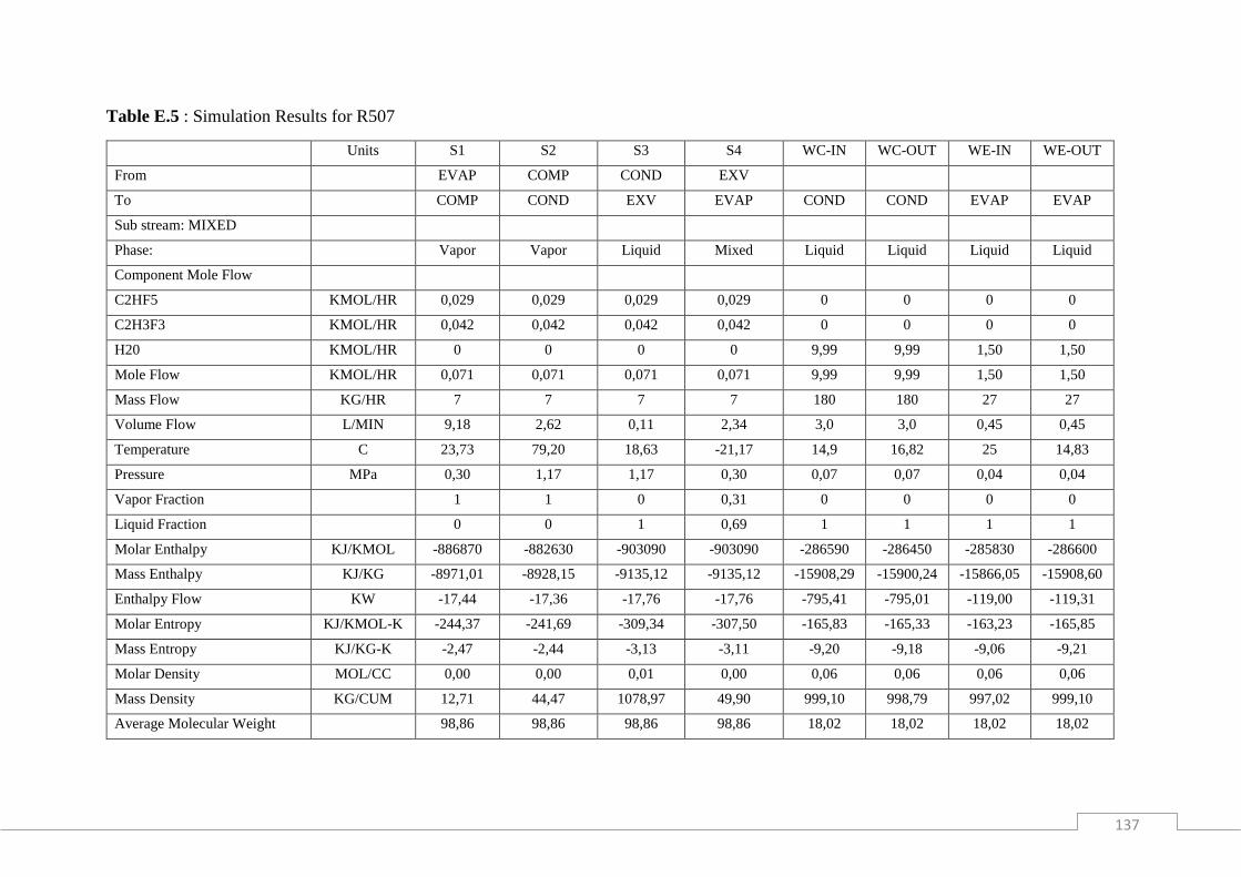
137
Table E.5 : Simulation Results for R507
Units S1 S2 S3 S4 WC-IN WC-OUT WE-IN WE-OUT
From
EVAP COMP COND EXV
To
COMP COND EXV EVAP COND COND EVAP EVAP
Sub stream: MIXED
Phase:
Vapor Vapor Liquid Mixed Liquid Liquid Liquid Liquid
Component Mole Flow
C2HF5 KMOL/HR 0,029 0,029 0,029 0,029 0 0 0 0
C2H3F3 KMOL/HR 0,042 0,042 0,042 0,042 0 0 0 0
H20 KMOL/HR 0 0 0 0 9,99 9,99 1,50 1,50
Mole Flow KMOL/HR 0,071 0,071 0,071 0,071 9,99 9,99 1,50 1,50
Mass Flow KG/HR 7 7 7 7 180 180 27 27
Volume Flow L/MIN 9,18 2,62 0,11 2,34 3,0 3,0 0,45 0,45
Temperature C 23,73 79,20 18,63 -21,17 14,9 16,82 25 14,83
Pressure MPa 0,30 1,17 1,17 0,30 0,07 0,07 0,04 0,04
Vapor Fraction
1 1 0 0,31 0 0 0 0
Liquid Fraction
0 0 1 0,69 1 1 1 1
Molar Enthalpy KJ/KMOL -886870 -882630 -903090 -903090 -286590 -286450 -285830 -286600
Mass Enthalpy KJ/KG -8971,01 -8928,15 -9135,12 -9135,12 -15908,29 -15900,24 -15866,05 -15908,60
Enthalpy Flow KW -17,44 -17,36 -17,76 -17,76 -795,41 -795,01 -119,00 -119,31
Molar Entropy KJ/KMOL-K -244,37 -241,69 -309,34 -307,50 -165,83 -165,33 -163,23 -165,85
Mass Entropy KJ/KG-K -2,47 -2,44 -3,13 -3,11 -9,20 -9,18 -9,06 -9,21
Molar Density MOL/CC 0,00 0,00 0,01 0,00 0,06 0,06 0,06 0,06
Mass Density KG/CUM 12,71 44,47 1078,97 49,90 999,10 998,79 997,02 999,10
Average Molecular Weight
98,86 98,86 98,86 98,86 18,02 18,02 18,02 18,02

138
Table E.6 : Simulation Results for R125
Updated
Units S1 S2 S3 S4 WC-IN WC-OUT WE-IN WE-OUT
From
EVAP COMP COND EXV
To
COMP COND EXV EVAP COND COND EVAP EVAP
Sub stream: MIXED
Phase:
Vapor Vapor Liquid Mixed Liquid Liquid Liquid Liquid
Component Mole Flow
H2O KMOL/HR 0 0 0 0 6,66 6,66 1,33 1,33
C2HF5 KMOL/HR 0,067 0,067 0,067 0,067 0 0 0 0
Mole Flow KMOL/HR 0,067 0,067 0,067 0,067 6,66 6,66 1,33 1,33
Mass Flow KG/HR 8 8 8 8 120 120 24 24
Volume Flow CUM/HR 0,38 0,13 0,007 0,11 0,12 0,12 0,024 0,024
Temperature C 20 68,34 21 -15,35 20 22,55 25 14,89
Pressure MPa 0,4 1,30 1,30 0,4 0,07 0,07 0,04 0,04
Vapor Fraction
1 1 0 0,32 0 0 0 0
Liquid Fraction
0 0 1 0,68 1 1 1 1
Solid Fraction
0 0 0 0 0 0 0 0
Molar Enthalpy KJ/KMOL -1101400 -1097500 -1116700 -1116700 -286210 -286020 -285830 -286590
Mass Enthalpy KJ/KG -9177,03 -9144,02 -9303,96 -9303,96 -15886,94 -15876,28 -15866,05 -15908,37
Enthalpy Flow KW -20,39 -20,32 -20,68 -20,68 -529,56 -529,21 -105,77 -106,06
Molar Entropy KJ/KMOL-K -265,41 -261,75 -325,37 -323,66 -164,51 -163,85 -163,23 -165,83
Mass Entropy KJ/KG-K -2,21 -2,18 -2,71 -2,70 -9,13 -9,10 -9,06 -9,21
Molar Density KMOL/CUM 0,18 0,53 10,11 0,63 55,41 55,38 55,34 55,46
Mass Density KG/CUM 21,11 63,33 1213,51 75,77 998,19 997,63 997,02 999,09
Average Molecular Weight
120,02 120,02 120,02 120,02 18,02 18,02 18,02 18,02
139
Appendix F: Simulation Procedure
Aspen Refrigeration Cycle Simulation Procedure
Getting Started
➢ Open the Aspen user interface, click on file then on new.
➢ With the Installed Templates highlighted on the left and blank simulation to the right,
select Create. Component selection platform pops up.
Properties
➢ On the component specification tab, specify all components to be used in the
simulation. On the third column with heading Component name type the chemical name
for the substance to be used in the simulation. Then click on find to recall the component
from the Aspen Database.
➢ If the component (substance) does not exist in the databank it can be added using User
Defined option.
➢ The sequence in which the components are specifications does not matter, they can be
specified in any order. When all the components have been entered then click next.
➢ Method specification template comes up, then selected the method to be used in the
simulation.In this case, REFPROP method is selected from a list of methods available
in Aspen database as it is the method selected for this study.
➢ The physical properties of the components selected can be viewed by clicking the
Retrieve Parameters Icon.
Simulation
➢ At the bottom left-hand corner of the user interface, a statement that notifies that
Required Properties Input Complete. Then click on Simulation Icon situated on the at
the bottom left corner.
➢ A blank Flowsheet comes up with a components bar at the bottom labeled model
palette. Then from the model palette select the four components of a refrigeration cycle
and drag them to the main-flowsheet.
➢ For the evaporator and the condenser –Click on Exchangers, Select HeatX then Gen
HT. Then rename the blocks as EVAP and COND respectively.
➢ For the compressor –Click on Pressure Changers, Select Compr, then ICON2
➢ For the expansion valve-Click on Pressure Changers, Select Valve, then VALVE2.

140
➢ For the connecting line click the arrow on the material, then on the Material Icon.
Connect on the component to the next to produce a closed cycle with HTF lines flowing
into and out of the heat exchange.
➢ Rename the streams and produce a complete flowchart as shown in Figure 7.11.
➢ To set the fix parameters on the component Right click on the component then select
Input or double click.
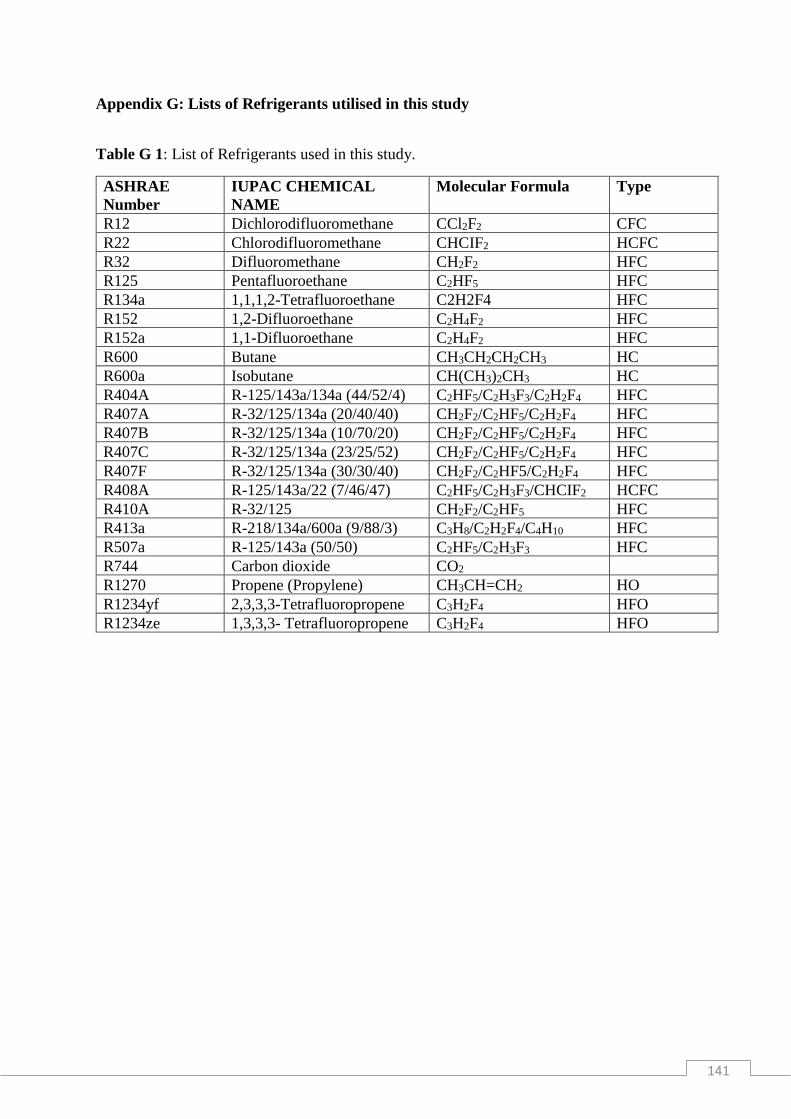
141
Appendix G: Lists of Refrigerants utilised in this study
Table G 1: List of Refrigerants used in this study.
ASHRAE
Number
IUPAC CHEMICAL
NAME
Molecular Formula Type
R12 Dichlorodifluoromethane CCl2F2 CFC
R22 Chlorodifluoromethane CHCIF2 HCFC
R32 Difluoromethane CH2F2 HFC
R125 Pentafluoroethane C2HF5 HFC
R134a 1,1,1,2-Tetrafluoroethane C2H2F4 HFC
R152 1,2-Difluoroethane C2H4F2 HFC
R152a 1,1-Difluoroethane C2H4F2 HFC
R600 Butane CH3CH2CH2CH3 HC
R600a Isobutane CH(CH3)2CH3 HC
R404A R-125/143a/134a (44/52/4) C2HF5/C2H3F3/C2H2F4 HFC
R407A R-32/125/134a (20/40/40) CH2F2/C2HF5/C2H2F4 HFC
R407B R-32/125/134a (10/70/20) CH2F2/C2HF5/C2H2F4 HFC
R407C R-32/125/134a (23/25/52) CH2F2/C2HF5/C2H2F4 HFC
R407F R-32/125/134a (30/30/40) CH2F2/C2HF5/C2H2F4 HFC
R408A R-125/143a/22 (7/46/47) C2HF5/C2H3F3/CHCIF2 HCFC
R410A R-32/125 CH2F2/C2HF5 HFC
R413a R-218/134a/600a (9/88/3) C3H8/C2H2F4/C4H10 HFC
R507a R-125/143a (50/50) C2HF5/C2H3F3 HFC
R744 Carbon dioxide CO2
R1270 Propene (Propylene) CH3CH=CH2 HO
R1234yf 2,3,3,3-Tetrafluoropropene C3H2F4 HFO
R1234ze 1,3,3,3- Tetrafluoropropene C3H2F4 HFO