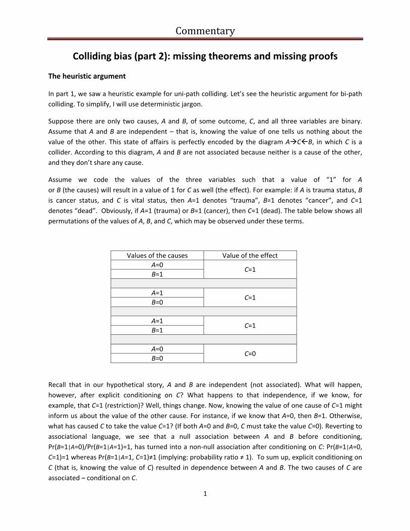
Commentary 

1  

Colliding bias (part 2): missing theorems and missing proofs 

The heuristic argument 

In part 1, we saw a heuristic example for uni‐path colliding. Let’s see the heuristic argument for bi‐path 

colliding. To simplify, I will use deterministic jargon. 

Suppose  there are only  two causes, A and B, of  some outcome, C, and all  three variables are binary. 

Assume  that A and B are  independent –  that  is, knowing  the value of one  tells us nothing about  the 

value of  the other. This  state of affairs  is perfectly encoded by  the diagram ACB,  in which C  is a 

collider. According to this diagram, A and B are not associated because neither  is a cause of the other, 

and they don’t share any cause. 

Assume  we  code  the  values  of  the  three  variables  such  that  a  value  of  “1”  for  A  

or B (the causes) will result in a value of 1 for C as well (the effect). For example: if A is trauma status, B 

is  cancer  status,  and  C  is  vital  status,  then  A=1  denotes  “trauma”,  B=1  denotes  “cancer”,  and  C=1 

denotes “dead”.  Obviously, if A=1 (trauma) or B=1 (cancer), then C=1 (dead). The table below shows all 

permutations of the values of A, B, and C, which may be observed under these terms. 

 

Values of the causes  Value of the effect 

A=0 C=1 

B=1 

 

A=1 C=1 

B=0 

 

A=1 C=1 

B=1 

 

A=0 C=0 

B=0 

 

Recall  that  in  our  hypothetical  story,  A  and  B  are  independent  (not  associated). What will  happen, 

however,  after  explicit  conditioning  on  C?  What  happens  to  that  independence,  if  we  know,  for 

example, that C=1 (restriction)? Well, things change. Now, knowing the value of one cause of C=1 might 

inform us about the value of the other cause. For  instance,  if we know that A=0, then B=1. Otherwise, 

what has caused C to take the value C=1? (If both A=0 and B=0, C must take the value C=0). Reverting to 

associational  language,  we  see  that  a  null  association  between  A  and  B  before  conditioning, 

Pr(B=1|A=0)/Pr(B=1|A=1)=1, has turned  into a non‐null association after conditioning on C: Pr(B=1|A=0, 

C=1)=1 whereas Pr(B=1|A=1, C=1)≠1 (implying: probability ra o ≠ 1).  To sum up, explicit condi oning on 

C  (that  is, knowing the value of C) resulted  in dependence between A and B. The two causes of C are 

associated – conditional on C. 

Commentary 

2  

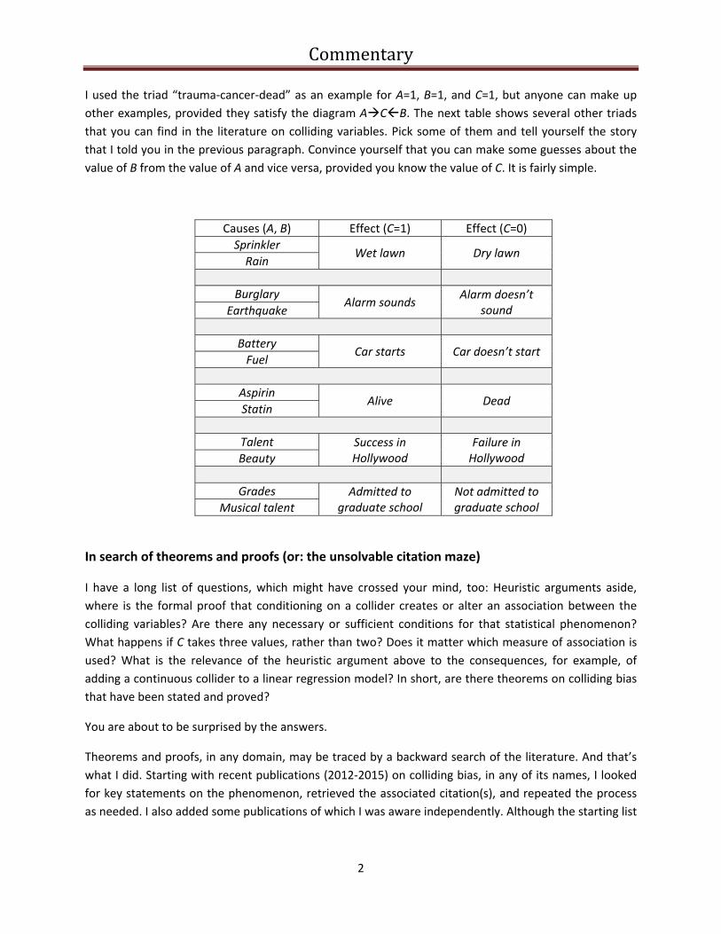
I used the triad “trauma‐cancer‐dead” as an example for A=1, B=1, and C=1, but anyone can make up 

other examples, provided they satisfy the diagram ACB. The next table shows several other triads 

that you can  find  in the  literature on colliding variables. Pick some of them and tell yourself the story 

that I told you in the previous paragraph. Convince yourself that you can make some guesses about the 

value of B from the value of A and vice versa, provided you know the value of C. It is fairly simple. 

 

Causes (A, B)  Effect (C=1)  Effect (C=0) 

Sprinkler Wet lawn  Dry lawn 

Rain 

   

Burglary Alarm sounds 

Alarm doesn’t sound Earthquake 

   

Battery Car starts  Car doesn’t start 

Fuel 

   

Aspirin Alive  Dead 

Statin 

   

Talent  Success in Hollywood  

Failure in Hollywood Beauty 

   

Grades  Admitted to graduate school  

Not admitted to graduate school Musical talent 

 

In search of theorems and proofs (or: the unsolvable citation maze) 

I have a  long  list of questions, which might have  crossed  your mind,  too: Heuristic arguments aside, 

where  is  the  formal proof  that conditioning on a collider creates or alter an association between  the 

colliding  variables? Are  there  any necessary or  sufficient  conditions  for  that  statistical phenomenon? 

What happens if C takes three values, rather than two? Does it matter which measure of association is 

used? What  is  the  relevance  of  the  heuristic  argument  above  to  the  consequences,  for  example,  of 

adding a continuous collider to a linear regression model? In short, are there theorems on colliding bias 

that have been stated and proved?  

You are about to be surprised by the answers. 

Theorems and proofs, in any domain, may be traced by a backward search of the literature. And that’s 

what I did. Starting with recent publications (2012‐2015) on colliding bias, in any of its names, I looked 

for key statements on the phenomenon, retrieved the associated citation(s), and repeated the process 

as needed. I also added some publications of which I was aware independently. Although the starting list 

Commentary 

3  

was neither exhaustive nor methodically sampled, some citation paths should have led to theorems and 

proofs. Sounds reasonable? 

Figure 1 shows the maze of citations (causality works in reverse to the direction of the arrows). Most of 

the paths end after one generation or two; some publications hang alone. Publications in a box seem to 

be promising roots, so I will examine them closely: what they say and what they cite, if anything. 

 

Figure 1. 

 

 

 

Hernan (2015) 

Hernan MA, Robins JM (2015): Causal Inference  (August 27, 2015) 

https://cdn1.sph.harvard.edu/wp‐content/uploads/sites/1268/2015/08/hernanrobins_v1.10.30.pdf 

(Accessed on January 14, 2016) 

Banack (2015)

Snoep (2014) Swanson (2014)Flanders (2014)

Sanni Ali (2013)

Jansen (2012) Sung (2012)

Cole (2010) Whitcomb (2009)Glymour (2008)

VanderWeele (2007)

Hernan (2004)

Greenland (2003)

Greenland (1999)

Pearl (1995)

Spirtes (1993)

Robins (2001) Pearl (2000)

Glymour (2005)

Hernan (2002)

Hernan (2015)

Commentary 

4  

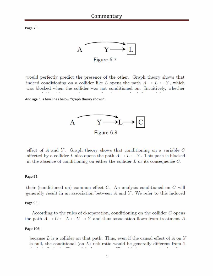
Page 75: 

 

 

And again, a few lines below “graph theory shows”: 

 

 

 

Page 95: 

 

 

Page 96: 

 

Page 106: 

 

Commentary 

5  

In summary, 

“graph theory shows” (page 75). No reference. 

“will generally result” (page 95). Only generally? No graph theory? 

 “according to the rules of d‐separation” (page 96). Graph theory has turned into rules 

 “would be generally different” (page 106). Back to “generally”. 

So which is it? A proved theorem in graph theory? A rule made by an anonymous ruler? Or just wishy‐

washy “generally”?  

 

Glymour (2008) 

Glymour MM, Greenland S. Chapter 12: causal diagrams. In Modern Epidemiology (3rd edition), 2008  

On page 187, we find a section heading on “rules”: 

 

And in that section we find the following rule: 

Page 188: 

 

So, which is it? “conditioning…opens the path at W”, or we only “expect conditioning on W…to create an 

X–Y association via W”? The first sounds like a theorem, whereas the second sounds like another version 

of “generally”. No reference is cited here, but at the very beginning of the chapter (Introduction) we are 

told that the rules are “grounded in mathematics”. 

 

And  at  the end of  the  introduction  (page 184), we  are  referred  to  two  references  that provide  “Full 

technical details of causal diagrams and their relation to causal inference”:  Pearl (2000) and Spirtes et al 

Commentary 

6  

(2001). Both books indeed contain lots of technical details, including theorems and proofs. Do they also 

contain theorems and proofs on the consequences of conditioning on a collider in every (or any) form of 

conditioning? If you find any, let me know the page number. 

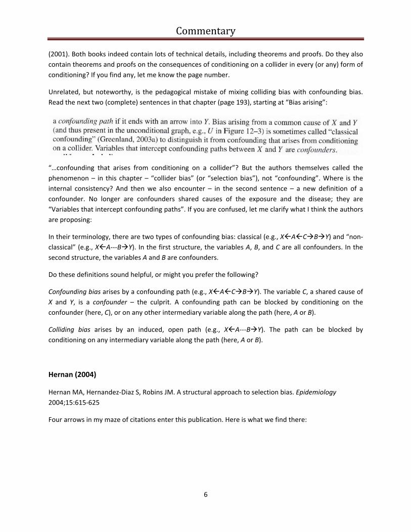
Unrelated, but noteworthy,  is  the pedagogical mistake of mixing colliding bias with confounding bias.  

Read the next two (complete) sentences in that chapter (page 193), starting at “Bias arising”: 

 

“…confounding  that  arises  from  conditioning  on  a  collider”?  But  the  authors  themselves  called  the 

phenomenon –  in  this chapter – “collider bias”  (or “selection bias”), not “confounding”. Where  is  the 

internal  consistency? And  then we  also  encounter  –  in  the  second  sentence  –  a new definition of  a 

confounder.  No  longer  are  confounders  shared  causes  of  the  exposure  and  the  disease;  they  are 

“Variables that intercept confounding paths”. If you are confused, let me clarify what I think the authors 

are proposing: 

In their terminology, there are two types of confounding bias: classical (e.g., XACBY) and “non‐

classical” (e.g., XA‐‐‐BY). In the first structure, the variables A, B, and C are all confounders. In the 

second structure, the variables A and B are confounders. 

Do these definitions sound helpful, or might you prefer the following? 

Confounding bias arises by a confounding path (e.g., XACBY). The variable C, a shared cause of 

X  and  Y,  is  a  confounder  –  the  culprit.  A  confounding  path  can  be  blocked  by  conditioning  on  the 

confounder (here, C), or on any other intermediary variable along the path (here, A or B). 

Colliding  bias  arises  by  an  induced,  open  path  (e.g.,  XA‐‐‐BY).  The  path  can  be  blocked  by 

conditioning on any intermediary variable along the path (here, A or B). 

 

Hernan (2004) 

Hernan MA, Hernandez‐Diaz S, Robins JM. A structural approach to selection bias. Epidemiology 

2004;15:615‐625 

Four arrows in my maze of citations enter this publication. Here is what we find there: 

 

 

 

Commentary 

7  

Page 615: 

 

Page 616: 

 

 

 

The phrase “formal  justification” should mean “theorems and proofs”.  If not,  I  fail to grasp  its precise 

meaning. References 13 and 14 (shown above) are promising roots in my maze of citations, so they will 

be examined later. 

 

Greenland (2003) 

Greenland S. Quantifying biases in causal models: classical confounding vs collider‐stratification bias. 

Epidemiology 2003;14:300‐306 

 

 

That’s a statement that sounds exactly like a theorem – actually, a strong theorem (“within at least one 

stratum”). So  reference  “1(pp17)”  should provide a proof. What do we  find  there? That’s  coming up 

next. 

Commentary 

8  

Pearl (2000) 

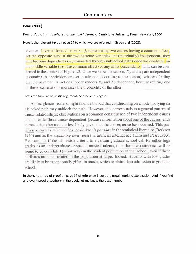
Pearl J. Causality: models, reasoning, and inference.  Cambridge University Press, New York, 2000  

Here is the relevant text on page 17 to which we are referred in Greenland (2003): 

 

That’s the familiar heuristic argument. And here it is again:  

 

In short, no shred of proof on page 17 of reference 1. Just the usual heuristic explanation. And if you find 

a relevant proof elsewhere in the book, let me know the page number. 

 

 

 

 

 

Commentary 

9  

Robins (2001) 

Robins JM. Data, design, and background knowledge in etiologic inference. Epidemiology 2001;11:313‐

320.  

 

 

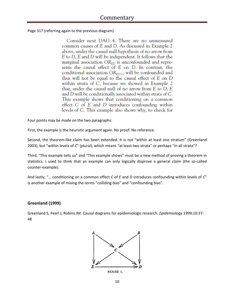
Page 315 

 

Page 316 (referring to DAG 4) 

 

By the way, the explanation here for the word “usually”(in “usually negatively associated”) has nothing 

to do with the case of explicit conditioning on C (restricting C to one value). 

 

 

 

Commentary 

10  

Page 317 (referring again to the previous diagram) 

 

Four points may be made on the two paragraphs: 

First, the example is the heuristic argument again. No proof. No reference. 

Second,  the  theorem‐like claim has been extended.  It  is not “within at  least one stratum”  (Greenland 

2003), but “within levels of C” (plural), which means “at least two strata” or perhaps “in all strata”? 

Third, “This example tells us” and “This example shows” must be a new method of proving a theorem in 

statistics.  I  used  to  think  that  an  example  can  only  logically  disprove  a  general  claim  (the  so‐called 

counter‐example). 

And lastly, “… conditioning on a common effect C of E and D introduces confounding within levels of C” 

is another example of mixing the terms “colliding bias” and “confounding bias”. 

 

Greenland (1999) 

Greenland S, Pearl J, Robins JM. Causal diagrams for epidemiologic research. Epidemiology 1999;10:37‐

48 

 

Commentary 

11  

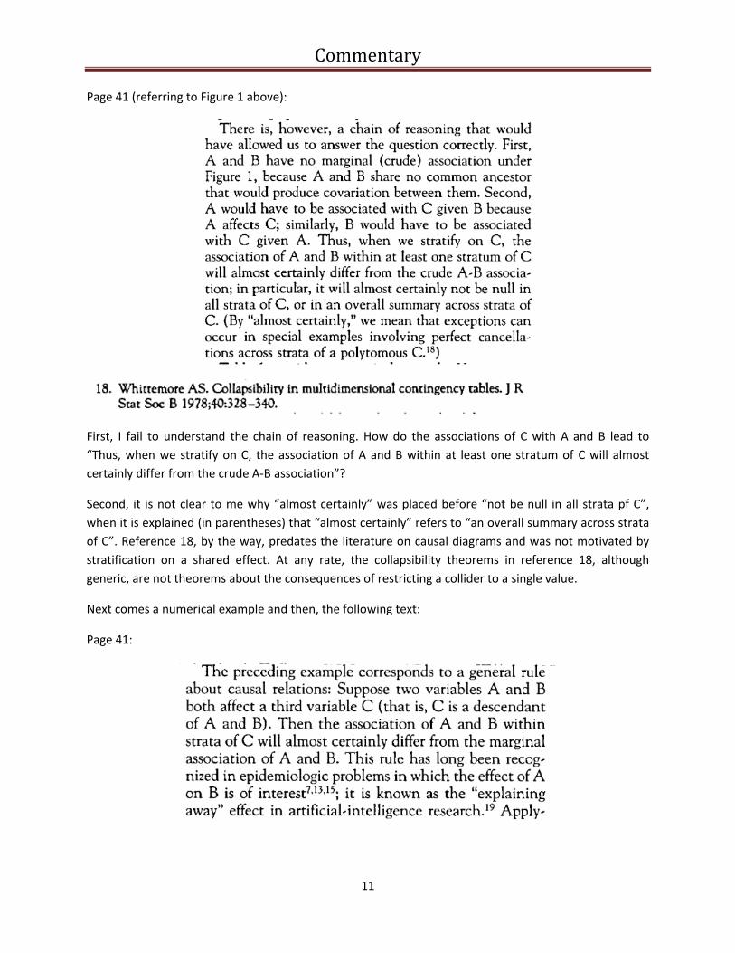
Page 41 (referring to Figure 1 above): 

 

 

First,  I  fail  to understand  the  chain of  reasoning. How do  the associations of C with A and B  lead  to 

“Thus, when we stratify on C,  the association of A and B within at  least one stratum of C will almost 

certainly differ from the crude A‐B association”? 

Second,  it  is not clear to me why “almost certainly” was placed before “not be null  in all strata pf C”, 

when it is explained (in parentheses) that “almost certainly” refers to “an overall summary across strata 

of C”. Reference 18, by the way, predates the  literature on causal diagrams and was not motivated by 

stratification  on  a  shared  effect.  At  any  rate,  the  collapsibility  theorems  in  reference  18,  although 

generic, are not theorems about the consequences of restricting a collider to a single value. 

Next comes a numerical example and then, the following text: 

Page 41: 

 

Commentary 

12  

So now  “the  association of A  and B within  strata of C will  almost  certainly differ  from  the marginal 

association of A and B”.    Is  it “almost certainly within strata”, or “almost certainly within at  least one 

stratum”? Or just “certainly within at least one stratum”? What is the presumed theorem? Or maybe it 

is  just “a rule” that “has  long been recognized  in epidemiologic problems”? One thing  is certain: all of 

these  imprecise  statements  could  not  have  originated  from  any  published,  proven  theorem(s). 

Moreover, if there was a proven theorem, we would undoubtedly have seen a reference. 

 

Pearl (1995) 

Pearl J. Causal diagrams for empirical research. Biometrika 1995;82:669‐710 

No text  is shown here, simply because there  is no relevant text to show. There  is a  lot on confounding 

bias in that article (e.g., section 3 “Controlling Confounding Bias”), and the theorems for a sufficient set 

for  conditioning  inevitably  take  into  account  the  phenomenon  of  colliding  bias. But  there  is  nothing 

explicit on colliding bias (or “selection bias”, or “collider bias”, or “explaining away effect”). In fact, none 

of these terms  is even mentioned. Since the key theme of the article  is “identifiability” – conditioning 

that  allows  bias‐free  estimation  of  an  effect,  given  a  graph  –  it  is  not  surprising  that  there  are  no 

theorems on the consequences of conditioning on a collider. The word “collider” is nowhere to be found 

in that article (although colliders are shown in Section 5.3, Figure 7, where non‐identifiable models are 

described.) 

 

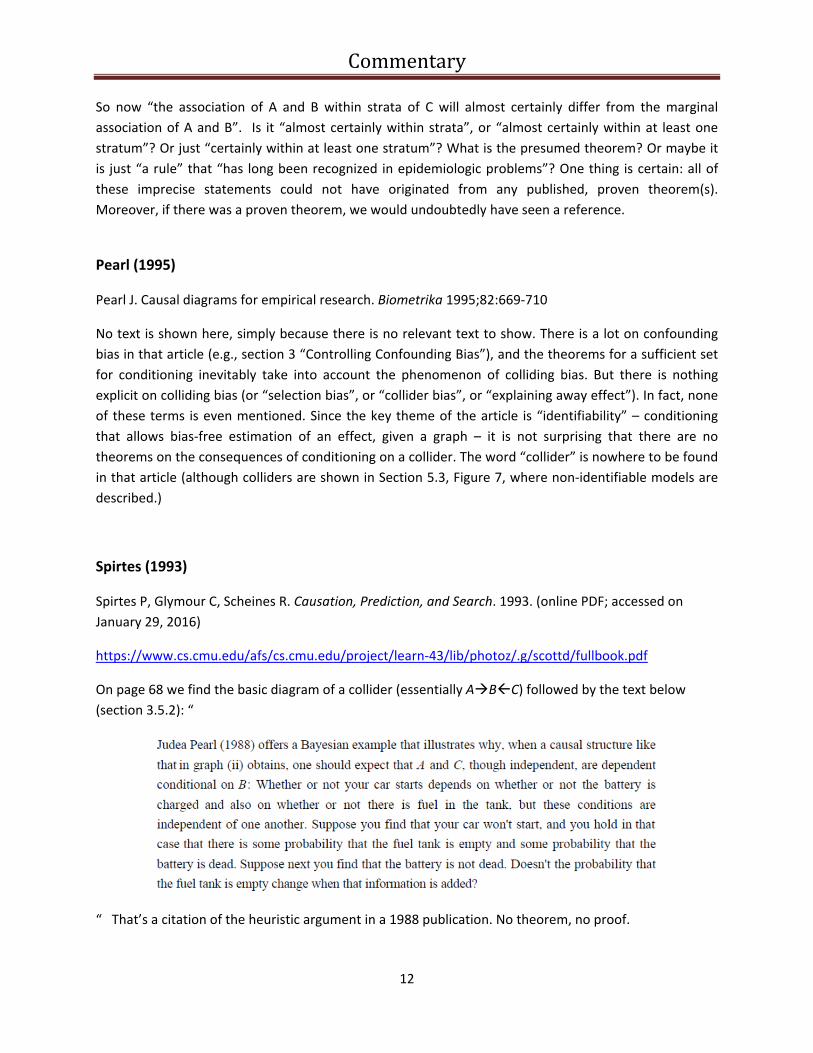
Spirtes (1993) 

Spirtes P, Glymour C, Scheines R. Causation, Prediction, and Search. 1993. (online PDF; accessed on 

January 29, 2016)  

https://www.cs.cmu.edu/afs/cs.cmu.edu/project/learn‐43/lib/photoz/.g/scottd/fullbook.pdf 

On page 68 we find the basic diagram of a collider (essentially ABC) followed by the text below 

(section 3.5.2): “ 

 

“   That’s a citation of the heuristic argument in a 1988 publication. No theorem, no proof.  

Commentary 

13  

And then on page 72, we find reference to the text above as follows: 

“That conditioning on a collider makes it active was noted in section 3.5.2 above.” 

The book contains many proofs of theorems and lemmas on causal diagrams, with special emphasis on 

the faithfulness condition.  Is there also a direct proof of a theorem on colliding bias? The notation is 

heavy, but I did not recognize one. 

 

My writing 

A small surprise at the end. I used to belong to the majority that believes that “brilliant minds must have 

proven the fundamentals”. So, I also contributed my share to the claims about theorems. Here are two 

examples: 

Shahar  E,  Shahar  DJ.  Causal  diagrams  and  the  logic  of  matched  case‐control  studies.  Clinical 

Epidemiology 2012;4:137‐144 [Corrigendum: Clinical Epidemiology 2014;6:59] 

Page 138: 

 

Yes, there are quite a few theorems on causal diagrams and expected dependence/independence 

between displayed variables. But are there stated theorems on the consequences of conditioning on a 

collider? If so, why do we encounter repeated heuristic explanations? Why does the maze of citations 

not end in a common reference of a theorem and a proof? 

Page 138 

 

 

 

And here is reference 2, followed by the relevant text: 

Shahar  E,  Shahar DJ  (2012):    Causal  diagrams  and  three  pairs  of  biases.  In:  Epidemiology    –  Current 

Perspectives  on  Research  and  Practice  (Lunet  N,  Editor). www.intechopen.com/books/epidemiology‐

current‐perspectives‐on‐research‐and‐practice, pp. 31‐62 

Commentary 

14  

Pages 37‐38 

 

 

“Formal  proofs  are  available”  on  colliding  bias?  I  assumed  so  –  carelessly  accepting  published 

statements  such  as  “For  a  formal  justification,  see  references…”  and  “graphical  rules…grounded  in 

mathematics”. In my defense (or rather, to my discredit), I did not cite any external reference.  

In part 3,  I hope  to  revisit  the  topic of effect modification  (mentioned above) as a prerequisite  for a 

newly  formed  association  after  conditioning  on  a  collider.  That’s  quite  interesting  (and  possibly  a 

theorem for some types of conditioning). 

 

References (in alphabetic order) 

Banack HR, Kaufman JS (2015). From bad to worse: collider stratification amplifies confounding bias  in 

the “obesity paradox”. European Journal of Epidemiology 30:1111‐4 

Cole SR, Platt RW, Schisterman  EF, Chu  H, Westreich  D, Richardson  D, Poole C  (2010).  Illustrating  bias 

due to conditioning on a collider. International Journal of Epidemiology 39:417‐20 

Flanders WD, Eldridge RC, McClellan WM (2014). A nearly unavoidable mechanism for collider bias with 

index‐event studies. Epidemiology 25:762‐764 

Glymour MM, Weuve J, Berkman LF, Kawachi I, Robins JM (2005). When is baseline adjustment useful in 

analysis of change? An example with education and cognitive change. American Journal of Epidemiology 

162:267‐278 

Glymour MM, Greenland S (2008). Chapter 12: causal diagrams. In Modern Epidemiology (3rd edition)  

Greenland S, Pearl J, Robins JM (1999). Causal diagrams for epidemiologic research. Epidemiology 10:37‐

48 

Commentary 

15  

Greenland S (2003). Quantifying biases  in causal models: classical confounding vs collider‐stratification 

bias. Epidemiology 14:300‐306 

Hernan MA, Hernandez‐Diaz S, Werler MM, Mitchell AA (2002). Causal knowledge as a prerequisite for 

confounding evaluation: an application to birth defects epidemiology. American Journal of Epidemiology 

155:176–84 

Hernan MA, Hernandez‐Diaz S, Robins JM (2004). A structural approach to selection bias. Epidemiology 

15;615‐625 

Hernan MA, Robins JM (2015): Causal Inference  (August 27, 2015) 

Jansen JP, Schmid CH, Salanti G (2012). Directed acyclic graphs can help understand bias in indirect and 

mixed treatment comparisons. Journal of Clinical Epidemiology 65:798‐807 

Pearl J (1995). Causal diagrams for empirical research. Biometrika 82:669‐710 

Pearl J (2000). Causality: models, reasoning, and inference.  Cambridge University Press, New York 

Robins JM (2001). Data, design, and background knowledge in etiologic inference. Epidemiology 11:313‐

320.  

Sanni Ali M, Groenwold RH, Pestman WR, Belitser SV, Hoes AW, de Boer A, Klungel OH (2013). European 

Journal of Epidemiology 28:291‐9 

Shahar  E,  Shahar  DJ  (2012).  Causal  diagrams  and  three  pairs  of  biases.  In:  Epidemiology    –Current 

Perspectives  on  Research  and  Practice  (Lunet  N,  Editor). www.intechopen.com/books/epidemiology‐

current‐perspectives‐on‐research‐and‐practice, 2012: pp. 31‐62 

Shahar  E,  Shahar DJ  (2012).  Causal  diagrams  and  the  logic  of matched  case‐control  studies.  Clinical 

Epidemiology 4:137‐144 [Corrigendum: Clinical Epidemiology 2014;6:59] 

Snoep JD, Morabia A, Hernandez‐Diaz  S, Hernan  MA, Vandenbroucke  JP  (2014).  Commentary:  A 

structural  approach  to  Berkson's  fallacy  and  a  guide  to  a  history  of  opinions  about  it.  International 

Journal of Epidemiology 43:515‐21 

Spirtes P, Glymour C, Scheines R (1993). Causation, Prediction, and Search, New York 

Sung VW (2012). Reducing bias in pelvic floor disorders research: using directed acyclic graphs as an aid. 

Neurourology and Urodynamics 31:115‐120 

Swanson SA, Robins JM, Miller M, Hernan MA (2015). Selecting on treatment: a pervasive form of bias in 

instrumental variable analyses. American Journal of Epidemiology 181:191‐197 

VanderWeele TJ, Robins JM  (2007).  Directed  acyclic  graphs,  sufficient  causes,  and  the  properties  of 

conditioning on a common effect. American Journal of Epidemiology 166:1096‐1104 

Commentary 

16  

Whitcomb BW, Schisterman EF, Perkins NJ, Platt RW (2009). Quantification of collider‐stratification bias 

and the birthweight paradox. Paediatric and Perinatal Epidemiology 23:394‐402 

 

 

 

Colliding bias (part 3): what theorems should we look for? (forthcoming)