1

COMBUSTION THERMODYNAMICS

Combustion Thermodynamics ...................................................................................................................... 1

Combustion ............................................................................................................................................... 1

Thermodynamics fundamentals ................................................................................................................ 2

Thermodynamics of mixtures ................................................................................................................... 4

Equilibrium ........................................................................................................................................... 4

Chemical potential expressions ............................................................................................................. 4

Thermal capacity averaging .................................................................................................................. 5

Water vapour condensation ................................................................................................................... 6

Thermochemistry ...................................................................................................................................... 6

Stoichiometry, extent and affinity ......................................................................................................... 7

Enthalpy of formation and absolute entropy ......................................................................................... 8

Heating value ........................................................................................................................................ 8

Maximum work ................................................................................................................................... 10

Adiabatic combustion temperature ..................................................................................................... 11

Equilibrium composition..................................................................................................................... 14

COMBUSTION THERMODYNAMICS

COMBUSTION

Combustion is a self-propagating exothermic oxidative chemical reaction, mostly in gas phase, producing

light, heat and smoke in a nearly-adiabatic flame front. The overall process in combustion is analogous to

those taking place in fuel cells and living-matter respiration, so that the same overall results apply in all

three cases, in spite of their details being so different; combustion is characterised by the very high

temperatures reached.

The practical goal in combustion study is the prediction of its performance, for a safe, efficient and clean

design and operation of fire-making devices, in terms of the multiple physico-chemical phenomena

involved; it is thence a prerequisite to analysis the latter. Those phenomena may be split in two groups:

equilibrium behaviour (what we need and what we get), and kinetics (how we get it; at what rate).

Combustion Thermodynamics focuses on the former physico-chemical phenomena: fuel/air ratios,

heating values, maximum work obtainable, exhaust composition, etc., whereas Combustion kinetics

focuses on mixing process, flame geometry, ignition, extinction, propagation, stability, etc.

The study of combustion is based on the more general subject of Thermodynamics of Chemical

Reactions, usually called Thermochemistry. We shall deal here only with the peculiarities of the

combustion reaction, i.e. with focus on the thermodynamics of a fuel-and-air gas-phase reaction.

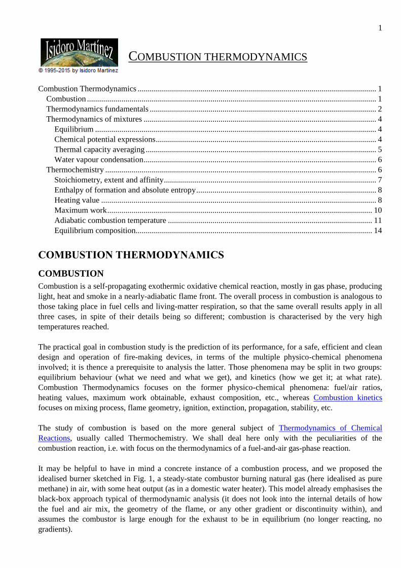
It may be helpful to have in mind a concrete instance of a combustion process, and we proposed the

idealised burner sketched in Fig. 1, a steady-state combustor burning natural gas (here idealised as pure

methane) in air, with some heat output (as in a domestic water heater). This model already emphasises the

black-box approach typical of thermodynamic analysis (it does not look into the internal details of how

the fuel and air mix, the geometry of the flame, or any other gradient or discontinuity within), and

assumes the combustor is large enough for the exhaust to be in equilibrium (no longer reacting, no

gradients).

2

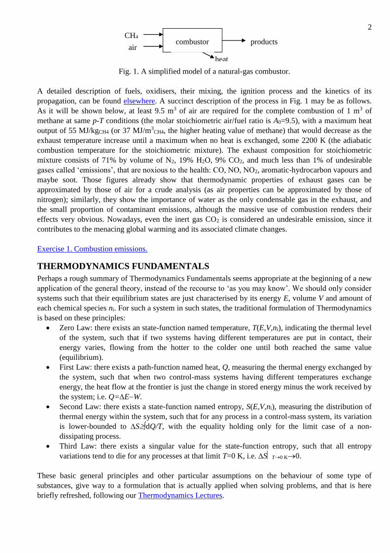
Fig. 1. A simplified model of a natural-gas combustor.

A detailed description of fuels, oxidisers, their mixing, the ignition process and the kinetics of its

propagation, can be found elsewhere. A succinct description of the process in Fig. 1 may be as follows.

As it will be shown below, at least 9.5 m3 of air are required for the complete combustion of 1 m3 of

methane at same p-T conditions (the molar stoichiometric air/fuel ratio is A0=9.5), with a maximum heat

output of 55 MJ/kgCH4 (or 37 MJ/m3CH4, the higher heating value of methane) that would decrease as the

exhaust temperature increase until a maximum when no heat is exchanged, some 2200 K (the adiabatic

combustion temperature for the stoichiometric mixture). The exhaust composition for stoichiometric

mixture consists of 71% by volume of N2, 19% H2O, 9% CO2, and much less than 1% of undesirable

gases called ‘emissions’, that are noxious to the health: CO, NO, NO2, aromatic-hydrocarbon vapours and

maybe soot. Those figures already show that thermodynamic properties of exhaust gases can be

approximated by those of air for a crude analysis (as air properties can be approximated by those of

nitrogen); similarly, they show the importance of water as the only condensable gas in the exhaust, and

the small proportion of contaminant emissions, although the massive use of combustion renders their

effects very obvious. Nowadays, even the inert gas CO2 is considered an undesirable emission, since it

contributes to the menacing global warming and its associated climate changes.

Exercise 1. Combustion emissions.

THERMODYNAMICS FUNDAMENTALS

Perhaps a rough summary of Thermodynamics Fundamentals seems appropriate at the beginning of a new

application of the general theory, instead of the recourse to ‘as you may know’. We should only consider

systems such that their equilibrium states are just characterised by its energy E, volume V and amount of

each chemical species ni. For such a system in such states, the traditional formulation of Thermodynamics

is based on these principles:

Zero Law: there exists an state-function named temperature, T(E,V,ni), indicating the thermal level

of the system, such that if two systems having different temperatures are put in contact, their

energy varies, flowing from the hotter to the colder one until both reached the same value

(equilibrium).

First Law: there exists a path-function named heat, Q, measuring the thermal energy exchanged by

the system, such that when two control-mass systems having different temperatures exchange

energy, the heat flow at the frontier is just the change in stored energy minus the work received by

the system; i.e. Q=EW.

Second Law: there exists a state-function named entropy, S(E,V,ni), measuring the distribution of

thermal energy within the system, such that for any process in a control-mass system, its variation

is lower-bounded to SdQ/T, with the equality holding only for the limit case of a non-

dissipating process.

Third Law: there exists a singular value for the state-function entropy, such that all entropy

variations tend to die for any processes at that limit T=0 K, i.e. ST0 K0.

These basic general principles and other particular assumptions on the behaviour of some type of

substances, give way to a formulation that is actually applied when solving problems, and that is here

briefly refreshed, following our Thermodynamics Lectures.

CH4

air products

heat

combustor

3

Details on the concept of energy, an additive and conservative function of kinetic and potential terms, can

be found aside, but the energy balance of a control mass system (one that cannot exchange mass with the

surroundings), and the perfect substance model for stored thermal energy, should be kept in mind:

E=Q+W (energy balance of a control mass) (1)

E=mcvT (stored thermal energy model for a perfect substance) (2)

Details on the concept of entropy, an additive non-conservative function measuring the internal

distribution of energy and other conservative properties, can be found aside, but its basic expression as a

function of other variables, and its particularisation for a perfect gas, should be retained:

mdfdQ dEdU pdV

ST T

(general expressions for entropy change) (3)

PGM

2 2

1 1

ln lnp

T pS mc mR

T p (entropy change in a perfect gas model) (4)

The combination of energy and entropy called exergy, measuring the maximum work obtainable from a

system, or the minimum work required to reach a global non-equilibrium state, is, for a control mass:

min 0 00univ

u u SW W E p V T S

(5)

Many thermodynamic variables (some extensive, others intensive) are used to simplify the analysis of

systems, amongst which enthalpy, thermal capacities, dilation and compressibility can be distinguished:

H≡U+pV, p

p p

s hc T

T T

, v

v v

s uc T

T T

,

1

p

V

V T

,

1

T

V

V p

(6)

But it must be remembered that, for pure substances, there are only two independent state variables, and

all others can be obtained by a combination of this two. In particular, the ideal gas equation of state is

omnipresent in all combustion studies:

pV=nRT with R=8.314 J/(mol∙K), or in the form p

RT or

RTv

p (7)

where the same symbol is used for the universal gas constant, Ru=8.3 J/(mol·K), and the particular gas

constant, R≡ Ru/M, for a gas of molar mass M. Most combustion processes take place within a control

volume, the combustor, and thus the equations developed in Control Volume analysis must be known,

particularly the omni-present steady-state mass and energy balances:

openings

0 em with m vA (8)

openings

0ee tQ W m h (9)

4

W being the shaft work input, Q the heat received, and hte the total specific enthalpy for each entrance

(or exit) with mass flow rate em . There are few combustion problems were equations (7-9) are not

involved.

Phase changes in pure substances are needed in combustion only to deal with pure liquid fuels, and it may

be enough to recall the equation for the vapour pressure curve, i.e. Clapeyron’s equation, more usually

used in the form of Antoine’s fitting:

lv

sat lv

hdp

dT Tv →

0 0

1 1ln lvhp

p RT T T

→

0unit

lnp B

ATp C

T

(10)

The Thermodynamics of mixtures is so important to combustion, that a more detailed summary is here

included.

THERMODYNAMICS OF MIXTURES

Combustion always involve a mixture, at least of a fuel and an oxidiser (usually air, another mixture

itself!), and the exhaust is always a mixture of burnt gases (except in the two ideal cases C+O2=CO2 and

H2+(1/2)O2=H2O). The general theory of Thermodynamics of Mixtures is developed aside, but the

important points to combustion are summarised here.

EQUILIBRIUM

An isolated mixture with conservative amounts of substance ni tends to reach an equilibrium state defined

by its entropy S(U,V,ni) being a maximum, what implies, in absence of external fields, that the

temperature T=U/S, pressure p=TS/V, and chemical potential for each conservative species

i=TS/ni, are uniform at equilibrium (in absence of external forces). Multi-phasic mixtures, and

mixture segregation due to external force fields, can be found aside.

CHEMICAL POTENTIAL EXPRESSIONS

The chemical potential, i, measures the tendency for an species to migrate, i.e. the escaping tendency of

chemical energy, in a similar way as temperature measures the escaping tendency of thermal energy, and

pressure the escaping tendency of compression energy. For a mixture in contact with an infinite

environment at T=constant and p=constant, as the ambient atmosphere, it is better to work with the Gibbs

function for the system G(T,p,ni)U+pVTS=HTS, instead of with the entropy of an isolated system. It

can be deduced, from Gibbs equation and Euler theorem for homogeneous functions, that G=ini; i.e.:

1

C

i i

i

G U pV TS H TS n

(11)

The differential form of the Gibbs function is used a lot in thermochemistry:

dG=SdT+Vdp+idni (12)

Several useful relations can be derived from it. First, the Gibbs-Duhem equation, subtracting (12) to the

total differential of (11), i.e.:

0=SdTVdp+nidi (13)

Second, the general dependence of i(T) and i(p); the former comes from the equality of the crossed

second derivatives 2G/(Tni)=si=2G/(niT)=i/T and from gi=hiTsi, what yields:

5

,

1

i

i

i

p n

T h

T

(14)

known as van’t Hoff equation; on the other hand, i(p) comes directly from the equality of the crossed

second derivatives 2G/(pni)=vi=2G/(nip)=i/p; i.e.:

, i

ii

T n

vp

(15)

For an ideal gaseous mixture, IGM, the chemical potential for an species i takes the form:

i(T,p,xi)IGM=i(T,p,1)+RTln(p/p)+RTlnxi (16)

indicating that the chemical potential varies with temperature according to the enthalpy function (13), and

varies with pressure logarithmically according to (12) and vi=RT/p, and varies with the molar fraction xi

also logarithmically.

THERMAL CAPACITY AVERAGING

The perfect gas model, besides the ideal gas equation of state (7), assumes constant thermal capacities cp,

simplifying the computations a lot; but a good averaged value of cp must be taken in combustion studies,

since cp varies considerably: e.g. for air at 300 K cp=1000 J/(kgK)=29 J/(molK), but at 3000 K cp=1240

J/(kgK)=36 J/(molK), and for water-vapour at 300 K cp=1900 J/(kgK)=34 J/(molK), but at 3000 K

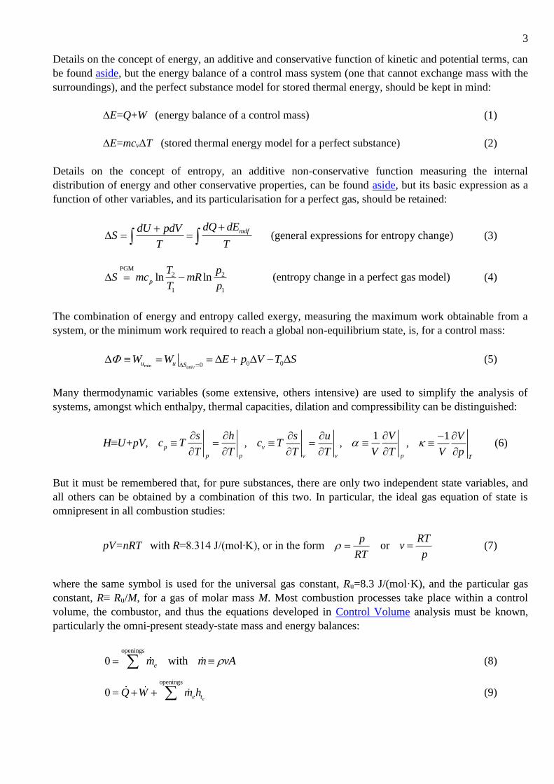
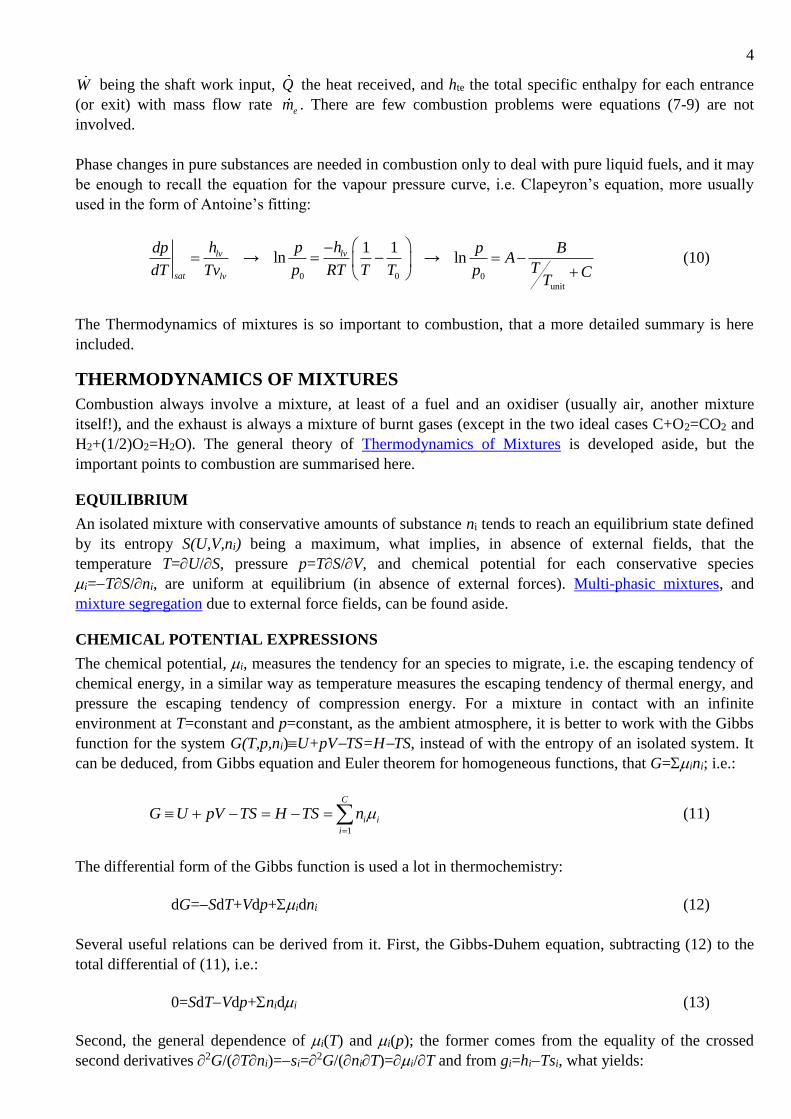
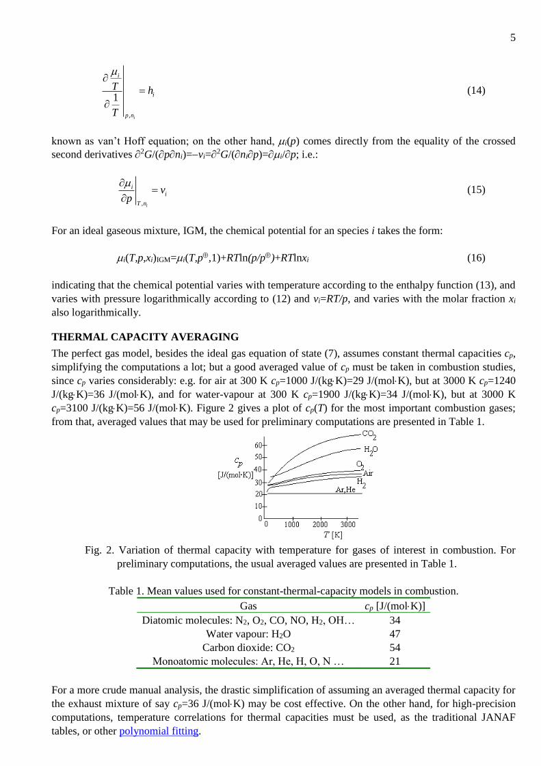
cp=3100 J/(kgK)=56 J/(molK). Figure 2 gives a plot of cp(T) for the most important combustion gases;

from that, averaged values that may be used for preliminary computations are presented in Table 1.

Fig. 2. Variation of thermal capacity with temperature for gases of interest in combustion. For

preliminary computations, the usual averaged values are presented in Table 1.

Table 1. Mean values used for constant-thermal-capacity models in combustion.

Gas cp [J/(molK)]

Diatomic molecules: N2, O2, CO, NO, H2, OH… 34

Water vapour: H2O 47

Carbon dioxide: CO2 54

Monoatomic molecules: Ar, He, H, O, N … 21

For a more crude manual analysis, the drastic simplification of assuming an averaged thermal capacity for

the exhaust mixture of say cp=36 J/(molK) may be cost effective. On the other hand, for high-precision

computations, temperature correlations for thermal capacities must be used, as the traditional JANAF

tables, or other polynomial fitting.

6

WATER VAPOUR CONDENSATION

Except in a few theoretical cases (C+O2=CO2, CO+(1/2)O2=CO2, S+O2=SO2, etc., that really take place

also with some water vapour), water is a genuine combustion product. Leaving aside the important

problem of acid rain formation in the combustion of sulfur-containing fuels, water is the only condensable

component in the products, being produced in such sizeable amounts (typically xH2O≈10%) that its

detailed account on mass and energy balances is of paramount importance).

Gaseous mixtures with a condensable component are dealt with in detail for the case of humid air aside.

Here we are concerned mostly with humid flue gases, but the approximation of non-condensable products

by air may be good enough; if not, the only modification is in the thermal capacity of non-condensable

gases, that should be changed from cp=1000 J/(kgK)=29 J/(molK) for air at about 15 ºC to cp=1100

J/(kgK)=32 J/(molK) for a typical exhaust mixture at about 50 ºC; the molar mass changes even less

because the increase due to the formation of carbon dioxide practically compensates with the decrease

due to water formation.

Recalling that liquid-vapour equilibrium, for ideal two-phase mixtures, implies uniform chemical

potential for each species I, one arrives at Raoult's law (see Mixtures):

xi,vap/xi,liq=pi*(T)/p (17)

i.e. the molar fraction of species i in the vapour phase, divided by the molar fraction in the liquid phase, is

equal to the vapour pressure for the pure i-component at that temperature, pi* (obtained from Clapeyron’s

equation or Antoine’s correlation), divided by the pressure of the mixture, p. It often helps to think of the

pressure of the mixture as the summation of partial pressures attributed to each i-component, pixi,vapp, so

that at liquid-vapour equilibrium pi=xi,liqp*(T).

For the case of one condensing species (water), the important equations are:

Maximum water-vapour fraction, xvap (notice that ‘vap’ now refers to the substance and not only

to the phase) dissolved in a given flue gas at given pressure p, and temperature T:

xvap=pi*(T)/p (18)

Dew point, i.e. condensing temperature, Tdew, for a given pressure p, and water molar fraction

xi,vap, it is solved from:

xi,vap=pi*(Tdew)/p (19)

Total pressure, p, for the two-phase system at equilibrium (humid exhaust plus condensate) at

temperature T:

p=pi,non-cond+pwater*(T) (20)

THERMOCHEMISTRY

A detailed thermodynamic treatment of generic reacting systems can be found aside. We will focus here

just in combustion reactions of simple fuels: hydrogen, carbon, and pure hydrocarbons (commercial fuels

are complex mixtures of hydrocarbons; see Fuel properties).

7

STOICHIOMETRY, EXTENT AND AFFINITY

A combustion process involves a set {Mi, i=1..C} of chemical species i, identified by their molecular

formula Mi (Mi is also used for their molar mass), undergoing a simultaneous set of chemical reactions

{Ri, i=1..R}, each one specified by its so-called stoichiometric equation:

' ''

1 1

C C

ir i ir i

i i

M M

or 1

0C

ir i

i

M

for r=1..R (e.g. H O H O2 2 2 12

) (21)

where the first form is preferred for kinetic studies when a direction in the process is implicit (it is said to

occur from reactants (left) converting into products (right), and sometimes an arrow is used instead of the

equal sign), whereas the last form is more simple for equilibrium studies where no direction is privileged.

In any case, (21) serves as the mass conservation equation if Mi is the molar mass of species i, and serves

to build the set of elementary conservation equations when the molecular form of Mi is considered. The i

are called stoichiometric coefficients for that reaction. Notice that the stoichiometric coefficients change

if one writes 0=2H2+O2-2H2O, or 0=H2+(1/2)O2-H2O, or 0=H2O-H2-(1/2)O2.

Most commercial fuels are hydrocarbons (chemical notation should be briefly refreshed, e.g. to

distinguish between n-octane and iso-octane). According to the stoichiometric ratio for full oxidation of a

fuel, air/fuel mixtures fed to a combustor are classified as:

Lean mixtures (little fuel content, excess of air).

Stoichiometric mixtures (with the precise or theoretical amount of fuel as established in a given

reaction as (21)).

Rich mixtures (more fuel than needed, but excess fuel will pyrolise to small-molecule fuels, and

only small molecules appear at the exhaust).

The ratio air-to-fuel in molar base is An≡nair/nfuel, and in massic base An≡nair/nfuel, although it is often

stated simply as A (but notice the values are different, though non-dimensional; e.g. theoretical air ratio

for methane, CH4+2·(O2+3.76·N2)=CO2+2·H2O+7.52·N2, is An=2·(1+3.76)/1=9.5, and

Am=AnMa/Mf=9.5·0.029/0.016=17, sometimes written as A=9.5 mola/molf=17 kga/kgf). The relative air-to-

fuel ratio is with respect to the stoichiometric air-to-fuel ratio A0; i.e. ≡A/A0 (now independent of the

molar or massic base). In the USA, the inverse of these functions are often used, namely the fuel-to-air

ratio, f=1/A (either in molar or massic base, as above), and the equivalence ratio =1/.

As for the products of combustion, the molar fractions are always used (also said 'volume fractions' since

they are the same with the ideal-gas mixture model predominant in combustion exhaust). Notice,

however, that, to avoid condensation of water inside the instruments, measurements of exhaust gases are

taken on a dry mixture that is obtained by passing the exhaust gases through desiccants (an ice bath is

often good enough, since most water is condensed and left behind).

When a control-mass mixture with initial composition ni0 reacts, the extent of the reaction at any later

time, (Greek letter xi, also called progress or degree of advancement of a reaction, a convenient

normalised mole-account system) is defined as:

n n

Mi i

i

i i0 for a given 0 = (22)

The extent of a reaction marks the state of progress; to measure the tendency to progress, the chemical

affinity, A, is defined:

8

A i i

i

C

1

(23)

such that Gibbs function variations are:

1

C

i i

i

dG SdT Vdp dn SdT Vdp Ad

(24)

the minus sign being introduced in the definition of A to ensure that natural evolution (entropy increase in

an isolated system, or Gibbs-function decrease in a system at T and p constant) corresponds to a positive

affinity, i.e. dG=Ad0 → progress, i.e. d/dt>0, only if A>0. It is important to notice that reactions with

negative affinities can naturally progress only at the expense of other reactions with positive and larger

affinities, since the real limit, at T and p constant, is dG=Ad0 for the whole set of reactions.

Although both, affinity and extent, are thermodynamic state functions, the reaction rate d/dt is not,

similarly to heat transfer. Reaction rates depend a lot on the presence of catalysts, that have no influence

on reaction equilibrium.

ENTHALPY OF FORMATION AND ABSOLUTE ENTROPY

Compounds are not conserved-entities in combustion, but atoms are. Thus, energy and entropy reference

states for each atom must be agreed in reacting systems, instead of the energy and entropy reference state

for each compound used in non-reacting systems. References are free to choose by the observer, but they

must necessarily be consistently related. The best references are:

Enthalpy reference: zero enthalpy is assigned to the most stable natural form of each chemical

elements at standard temperature and pressure (T=298 K and p=100 kPa). Enthalpies for non-

elementary species at standard temperature and pressure, called standard enthalpies of formation,

hf, are experimentally measured (usually by calorimetry, most of the times indirectly) and

tabulated. Enthalpy of an species at other temperature and pressure are computed from the general

relation dh=cpdT+(1T)vdp, according to the model used (e.g. for perfect gases h=hf+cp(TT)).

Entropy reference: zero entropy is assigned to each species (not just to each elementary species but

compounds too) at 0 K and any pressure, since it is an experimental fact explained by information

theory that entropy changes in the limit T0 also tend to zero. Entropy values at the standard state

(T=298 K and p=100 kPa), known as absolute standard entropies, s, are computed by

integration of experimentally measured (usually by spectrometry) thermal capacity data, according

to ds=(cp/T)dTvdp, and tabulated.

It is customary to include in the thermochemical tabulation not only hf and s, but also the standard

Gibbs function of formation of compounds from their elements, gf, although it is redundant since:

g h T sf f i i

i

C

1

for the reaction of formation of the compound: 0= i iM . (25)

HEATING VALUE

The standard practical heating value (PHV, also called practical calorific value, PCV) of a fuel is defined

as the heat transfer to cooling water in a Junkers-type calorimeter, i.e. a flow calorimeter with inputs (fuel

and air mixture, and cooling water) and output approaching standard conditions (298 K and 100 kPa), i.e.

the specific combustion enthalpy, hPHV (or its molar value). The fuel is burnt with excess air for complete

combustion, since the heating value is independent of excess air, while the cooling flow-rate is traded off

for best resolution (least uncertainty in w w w f PHVQ m c T m h ).

9

However, in order to provide a common reference to allow direct combination of heating values for

several reactions, a theoretical standard is defined by assuming that inlet and outlet flows run through

separated pipes for each pure chemical species. Thus, a so called standard higher heating value (HHV or

hHHV, sometimes known as high calorific value HCV) is defined as the heat release to the ambient when

fuel, oxidiser and products flow at 298 K, 100 kPa and species-separated), and computed by adding the

latent heat of the water-vapour (exiting the calorimeter above-mentioned), to the PHV. For instance, the

HHV for methane is (from the Combustion Data Table) hHHV=890 kJ/mol (hHHV=55 MJ/kg), meaning that

if a steady flow of methane is made to burn with air (or oxygen) at 100 kPa, both inlets (methane and air)

being at 298 K, and the outlet is cooled to 298 K, and only CO2 and H2O were produced and all the water

in the exhaust were condensed, 890 kJ by mole of methane will be released to the ambient (55 MJ by kg

of methane). In practice, there will be just one tail-pipe and at 25 ºC the water will be some 95%

condensed (forming a mist of micrometric droplets) and some 5% dissolved in the gas stream, and some

traces of unburnt hydrocarbons and possibly soot will also show up in the exhaust, and the measured

heating value would be slightly smaller.

However, for applications where the exhaust gases are above their dew point (a very common situation

since the exhaust dew point is typically below 60 ºC), it is advantageous for the calculations to establish a

different standard, called lower heating value (LHV or hLHV), that assumes all water exits at 100 kPa and

25 ºC but in the gaseous state (a virtual state not possible in practice for pure water); thus, the LHV is

equal to the HHV minus the vaporisation enthalpy of the exhaust water at 25 ºC (2.44 MJ/kg or 44 kJ/mol

of water produced). For instance, for methane, its combustion being CH4+2O2=CO2+2H2O, the LHV is

hLHV=890244=802 kJ/mol. Care is needed when using tabulated heating values, to know if they are

HHV or LHV.

Notice that the heating value of a fuel depends on input and output conditions and the path followed; heat

is a path variable, not a state function; HHV and LHV are defined as state functions, the negative of the

reaction enthalpy (hLHV=hr,comb), being for a given constant-pressure process. Fortunately for combustion

reactions, the heat release is practically independent on pressure, and depends very little with

temperature; even the difference between burning at constant pressure or at constant volume is not

significant. Notice also that the heating value of a fuel must be understood as the heat released in its

combustion with air (or any inert mixture with oxygen). Finally, recall that it has no sense to talk about

the 'energy content' of a fuel or of any other system, since energy is only defined between two states of a

closed system, by EW|Q=0; similarly, heat is only defined as energy transfer through an impermeable

boundary, by QEW.

For combustion at constant pressure, be it in a flow system (the most usual case) or in a control mass (e.g.

in an ideal Diesel cycle), the energy balance is:

Q=H=nfuelhHHV (26)

assuming all water is in condensed form. For combustion at constant volume of a control mass (e.g. in an

ideal Otto cycle), the energy balance is Q=E=U, but since the available data are enthalpies,

Q=(HpV)=HVp. If there is no condensed matter, i.e. for initial and final gaseous states, pV=nRT

and Q=HVp=H(nfinalninitial)RT; for instance, if 1 mol of CO is burnt at constant pressure in air

at 298 K and 100 kPa, the heat release is hHHV=hLHV=283 kJ/mol, whereas if the initial state is the same

but the burning is inside a rigid vessel at constant volume, the heat release may range from 283 kJ/mol for

a very diluted mixture to 283103+(11.5)8.3298=282 kJ/mol for an stoichiometric CO/O2 mixture. If

there is some condensed matter, either initially or at the end, a more involved analysis is required,

although, if the saturation pressure of the condense matter at the standard temperature is small, the same

equation as for gaseous mixtures may be applied just considering the non-condensed species; for instance,

10

if 1 mol of H2 is burnt at constant pressure in air at 298 K and 100 kPa, the heat release would be

hHHV=286 kJ/mol if the exhaust water were fully condensed, hLHV=242 kJ/mol if all the exhaust water

were in its vapour state, or a value close to the HHV in the practical case, whereas if the initial state is the

same but the burning is inside a rigid vessel at constant volume, the heat release may range from 242

kJ/mol for a very diluted gaseous mixture, to 286103+(01.5)8.3298=284 kJ/mol for an stoichiometric

H2/O2 mixture, that would produce near-zero gaseous moles. In summary, the heat release slightly varies

from constant pressure to constant volume combustion, the larger variation being with the physical state

of water at the end: for long-chain hydrocarbons the LHV is 6.5% lower than the HHV, the difference

increasing with decreasing carbon content (6.9% for C8H18, 9.1% for CH4 and 15.4% for H2).

All the above-defined heating values are global values for a non-equilibrium combustion process between

the initial and the final states quoted, but no difference is found if the instantaneous equilibrium changes

are introduced and the heating value is defined as the enthalpy of reaction (changed of sign because the

assumed direction for the heat release), i.e.

HHV

1 1 fuel,in,

C Ci i

r i i

i ip T

n hHh h h

n

and

2LHV HHV H O lvh h v h (27)

i.e. the ratio of the change of the enthalpy of a reacting system at equilibrium to the change in the extent

of reaction when an infinitesimal advance in the extent of the combustion reaction (scaled per unit of

amount of fuel) takes place. Similarly, the heat release at constant volume can be identified with the

internal energy of reaction at constant volume, or with the internal energy of reaction at constant pressure

for the case: U/|V,T=U/|p,T+U/p|,Tp/|V,T. The value for the molar enthalpy of water, for the

liquid-to-vapour phase change at T=298 K is hlv=44.0 kJ/mol=2442 kJ/kg.

MAXIMUM WORK

A combustion process may exchange both heat and work with the surroundings, only heat, only work, or

nothing of the two. The energy balance of the combustor relates the heat and work flows with the

entrance and exit temperatures.

The work obtainable from the combustion of a fuel depends on the actual process (as does the heat

release); if the combustion is performed in a rigid open chamber (as in a gas-turbine), no work will be

produced (at the combustion chamber), but if it is performed in a chamber with moving parts (as in a

reciprocating engine), some work will be produced. The maximum obtainable work, or the minimum

required work to reverse the process, for a steady process in the presence of an environment at

temperature T0 is the change in flow-exergy from inlet to outlet, =htT0s, that for standard

conditions is:

wmin==gr

=hrTsr

=ihf,iTisi

for a given 0= i iM (28)

where hf,i are standard enthalpies of formation of the participating compounds i=1..C, and si

their

absolute standard entropies. For instance, for the theoretical combustion of methane with oxygen,

CH4+2O2=CO2+2H2O, =gr=hr

Tisi=890103298(214+2701862205)=817103 J/mol,

i.e. 817 kJ/mol of work might be produced (the remainder to the heating value being evacuated as heat, on

account of the energy balance q+w=ht). Similarly, for H2+(1/2)O2=H2O a maximum of

=286103298(701310.5205)=237103 J/mol, i.e. as much as 237 kJ/mol of work might be

generated. If an energy efficiency is defined as the quotient between work produced and heating value,

the maximum efficiency would be 0.92 for methane and 0.83 for hydrogen (but mind that it would be

1.002 for carbon).

11

Recall here that there is a small difference between the maximum work obtainable from combustion and

the maximum work obtainable from the fuel (in spite of ambient-air having no exergy), because the

streams (to be considered separate components, since the thermochemical values refer to separate

streams) have some chemical exergy relative to the atmosphere, even when at T and p. For instance, the

maximum work obtainable from methane is CH4=831 kJ/mol (against the 817 kJ/mol above), computed

by adding the exergy of one mole of carbon dioxide, CO2=20 kJ/mol, and two moles of water,

H2O=1.3 kJ/mol, and subtracting the exergy of two moles of oxygen,

O2=3.9 kJ/mol, to the exergy of

the CH4+2O2=CO2+2H2O reaction, |r|=817 J/mol. Similarly, the exergy of hydrogen at the standard

state is H2=236 kJ/mol, to be compared with the exergy from H2+(1/2)O2=H2O, |

r|=237 J/mol.

Although an indirect realisation of the same global reaction can approach that maximum work, as in fuel

cells, direct combustion processes cannot approach those values. To begin with, if a constant-pressure

combustion process (the difference with a constant-volume process being small) were very slow, the heat

release would just dissipate to the environment without any possible work, i.e. all the exergy of the

reaction would be lost by entropy generation inside. If the process is rapid, as most combustions really

are, it may be assumed adiabatic to a first approximation, the heating value being spent in heating the

exhaust gases themselves instead of in heat transfer to another medium; no work is actually produced, but

some work may be obtained afterwards, since the exhaust is hotter than the environment.

To evaluate the maximum work obtainable from the adiabatically burnt gases, its exergy, one must

computed the flow exergy, =htT0s, of the hot exhaust stream relative to the atmosphere. It is good

enough to retain just the thermomechanical exergy, since the chemical exergy of dilution into the

atmosphere is much smaller. For hydrogen at standard conditions, for instance, the maximum obtainable

work (236 kJ/mol in an ideal fuel cell) is reduced to some 170 kJ/mol in the adiabatic exhaust at 100 kPa

and 2480 K after isobaric combustion of hydrogen with stoichiometric air, or to some 180 kJ/mol in the

adiabatic products at 870 kPa and 2950 K after isochoric combustion with stoichiometric air, due to the

unavoidable entropy generation inherent to the combustion process (entropy increase without entropy

flow).

Burning with pure oxygen increases the temperature of the adiabatic exhaust and thus its exergy. For

instance, in the case of H2/O2, some 190 kJ/mol of exergy per mole of hydrogen may be obtained from the

very hot adiabatic exhaust at some 4000 K and 100 kPa (difficult to compute because of dissociations). In

spite of this advantage of higher temperatures (already discovered by Carnot in the most general case),

practical combustion is most of the times with common air, even in some excess to further decrease the

temperature achieved, since common materials cannot withstand such high temperatures.

ADIABATIC COMBUSTION TEMPERATURE

The adiabatic model very accurately predicts homogeneous combustion temperatures in gas phase,

because of the very poor thermal conductivity of gases and the low speed (<0.5 m/s laminar burning

speed for ordinary hydrocarbon/air mixtures). The adiabatic model, however, overestimates the

temperature in the case of high radiation emission in non-premixed flames, and for high speeds flows

relative to solids (as in afterburner heat-exchangers).

The adiabatic temperature is a thermodynamic state variable that results from the conversion of internal

chemical energy to internal thermal energy after the combustion process takes place, and depends on the

actual fuel and oxidiser (e.g. CH4/air), their ratio (e.g. lean, stoichiometric or rich mixtures), their initial

thermodynamic state (e.g. premixed gases at 298 K and 100 kPa, although energies associated to mixing

and pressure are negligible), and the type and proportions of the compounds formed. It can be measured

at the exhaust of an adiabatic combustor, or just after a flame, but the practical difficulties in ensuring

12

minimal heat losses, particularly from the thermometer probe, render a theoretical computation more

precise that the actual measurement.

The problem with the computation is that the type and proportions of the compounds formed must be

known, what is partially solved assuming a set of compounds dictated by experience, and assuming that

they are in thermodynamic equilibrium at that pressure and temperature. But, even for the simplest case

of a constant-pressure combustion process (very good for open combustors since the pressure only rises

some 2% after a deflagration), the temperature is the unknown result and thus the equilibrium

composition cannot be directly computed, yielding an implicit and stiff algebraic mathematical problem.

The energy balance for a generic reactor is:

openings openings

, ,

1 1 1 1

d( )

d

C C

j j j ij f i ij i f i

j j i i

EW Q n h W Q n x h x h h

t

(29)

where the enthalpy contributions at each opening j is split in a chemical part (proportional to the molar

fraction i of each chemical component of standard enthalpies of formation hf,i, and a thermal part (from

the standard state to their actual state at the opening) of the participating compounds i=1..C. Notice that

the components are assumed known at entry and exit openings, but their molar fractions may be functions

of the temperature and pressure (e.g. when there is chemical equilibrium at an exit).

A drastic simplification of the energy balance occurs if one assumes complete combustion, because then

one can resolve the exhaust composition independently of temperature. This approach is useful for

combustion of lean mixtures in air, but not for combustion in pure oxygen where temperatures are higher.

With this simplification the adiabatic temperature for a stoichiometric H2/air mixture, for instance, is

computed to be 235050 K, in good agreement with a measure of 2300100 K, whereas the adiabatic

temperature for a stoichiometric H2/O2 mixture is computed to be 5400200 K, in clear disagreement

with a measure of 3000100 K.

With this complete-oxidation model, separating the entry flows and the exit flows, assuming 0W (no

work input/output through the impermeable walls), and assuming there is no phase change from the

standard state to the actual input or output states (see below), the energy balance for a steady state

combustor is

entry exit

1 1

0 ( ) ( )i i

C C

i i i p i i i p

i i

Q n x h x c T T n x h x c T T

(30)

Notice that water must be treated as an ideal gas to apply (30); otherwise, the enthalpy of phase change

must be added.

The actual mass balance or, better, molar balance for a combustor may be established in different ways,

according to the scale of amount of substance chosen. The main choices to write the so called mixture

equation are: per unit amount-of-substance of input stream, per unit amount-of-substance of output

stream, and per unit amount-of-fuel in the input stream. The last two usually take the form:

1

C

fuel air other i i

i

aM bM cM x M

and 1

C

fuel air other i i

i

M AM BM M

(31)

13

where a, b, c, A and B are numeric factors (A=b/a is the air/fuel ratio), Mi the molar masses of each

component (associated to the molecular formula stated; e.g. aC+bAir=xCOCO+xCO2CO2+xO2O2+xN2N2), xi

are the molar fractions in the exhaust (xi=1), and i are the amounts of exhaust species per unit amount

of fuel (not the stoichiometric coefficients).

Choosing the first option in (31), i.e. per unit amount-of-substance exiting, the energy balance (30) with

the definition of LHV in (27), yields:

exhaust

1

0 ( ) ( ) ( ) ( )fuel air other i

C

fuel p air p other p i i p

i

q a h c T T b h c T T c h c T T x h c T T

exhaust

LHV

1

( )( ) ( )fuel air other i

C

p p p in i p out

i

q ah ac bc cc T T x c T T

(32)

which can be read as follows: the thermal energy in the exhaust stream (the last term) is the contribution

of the external heat added through the walls per unit of exhaust q (zero for an adiabatic process), plus the

chemical heating value of the fuel input (the lower heating value, hLHV, since water is taken as a gas), plus

the thermal energy in the intake stream.

The adiabatic combustion temperature is obtained from (32) with q=0:

exhaust

LHV LHV

1

( )( )fuel air other

air

i

p p p in

ad C

pi p

i

ah ac bc cc T T ahT T T

cx c

(33)

where the last simplification (a most crude approach) neglects the thermal enthalpy input, and

approximates the thermal properties of the exhaust gas mixture by those of air, i.e. cp=1000 J/(kgK)=29

J/(molK) for cold air, or better cp=34 J/(molK) to account for the growth of thermal capacity with

temperature. Of course, the best precision is obtained with the integration cp/T)dT instead of the

approximation cpT in (30), but the first form of (33) with cp=34 J/(molK) for any diatomic molecule,

cp=47 J/(molK) for water vapour, and cp=54 J/(molK) for carbon dioxide (Table 2), is thought to be the

best compromise on precision/effort for non-programmed computations.

One may wonder why all vales of the maximum adiabatic combustion temperature in air are so close

(2300200 K, from combustion data Table), in spite of the widely different heating values (e.g. hLHV=10

MJ/kg for CO and hLHV=(1422.4)=140 MJ/kg for H2). A simple explanation can be found for

hydrocarbons, CnHm; their LHV may be approximated by the LHV of nC+(m/2)H2, which is

(n·394+m·242/2) kJ/mol. The adiabatic jump is TadT=hLHV/nicp,air, and it happens that the amount of

substance of the products varies almost proportional to the molar heating value. For the complete

stoichiometric combustion in air, CnHm+(n+m/4)·(O2+3.76N2)=nCO2+(m/2)H2O+3.76·(n+m/4)·N2, and

taking a mean value cp,air=40 J/(mol·K) for the exhaust gas, the total mole number in the products is

n·(1+3.76)+m·(1/2+3.6/4), which makes TadT=(n·394+m·121)/(n·0.190+m·0.058) K, a biparametric

function almost constant, of value TadT2000 K.

When dissociation is important due to the high temperatures associated to near-stoichiometric

combustion, or due to lack of oxygen in rich flames, computation of adiabatic temperatures is coupled to

computation of equilibrium composition. The effect of pressure on adiabatic temperature is through its

effect on equilibrium composition: at high pressure dissociation is negligible and the complete-

combustion adiabatic temperature gets its highest value, whereas reducing the pressure increases

dissociation in accordance with Le Châtelier principle, lowering adiabatic temperature.

14

EQUILIBRIUM COMPOSITION

The intake to a combustor is not at equilibrium (it would not react if it were), although it may be

considered at a metastable equilibrium (it would not react if not ignited), or even at separate fuel and air

inlets at their own equilibrium conditions before mixing. The exhaust from a combustor may be at

equilibrium (not with the surroundings but within itself, i.e. in chemical equilibrium at a given T and p), if

the combustion process has had time enough to develop completely. In practice, there are always some

partial reactions so slow that they do not reach equilibrium in the times considered, as for some trace

contaminants, but the assumption of perfect chemical equilibrium is a very good approximation to the

overall real combustion process, and, on top of that, serves to explain why a further simplification, the

complete combustion model, is an acceptable approximation to many combustion processes.

Chemical equilibrium in absence of external force fields implies no gradient of chemical potential, i=0,

for each component i=1..C, and no affinity to go on, Ar=0, for each reaction r=1..R. The latter establishes

a relation between molar fractions in the equilibrium composition xi, and T and p, for a given reaction

0=iMi, that for a reacting ideal gas mixture is (see Chemical reactions):

1

( , ) exp 1

i i

i

Cr r

i

i

g hp p Tx K T p

p p RT RT T

(34)

where the approximation lnK=A+B/T for the reaction constant K has been applied, and the constants gr

(standard Gibbs function of reaction) and gr (standard enthalpy of reaction) are computed from the

standard enthalpies and Gibbs functions of formation by:

1 1

,i i

C C

r i f r i f

i i

h h g g

(35)

For systems that are not at equilibrium yet, the ratio calculated from the mass-action law is called a

reaction quotient Q. The Q-values of a closed system have a tendency to reach a limiting value over time,

the equilibrium constant K.

Back to Combustion