Embed Size (px)
Citation preview

NASA Conference PiJlication 2433
CombustionFundamentals
NASA-Chinese Aeronautical
Establishment (CAE) Symposium
Proceedings of a symposiumheld at NASA Lewis Research Center
Cleveland, Ohio
September 23-27, 1985
https://ntrs.nasa.gov/search.jsp?R=19870010834 2018-07-17T19:22:10+00:00Z

NASA Conference Publication 2433
/
J CombustionFundamentals
NASA-Chinese Aeronautical
Establishment (CAE) Symposium
Proceedings of a symposiumheld at NASA Lewis Research Center
Cleveland, Ohio
September 23-27, 1985
National Aeronautics
and Space Administration
Scientific and Technical
information Branch
1986

FORENORD
In September and October of 1985 Vice President Zhang Cht of the ChineseAeronautical Establishment led a delegatlon of management and technical spe-cialists to the United States. Arrangements for the delegation were supervisedby Lavonne Parker of NASA. Included In the activities of this delegation wasthe NASA - Chinese Aeronautical Establishment (CAE) Symposium on CombustionFundamentals at the NASA Lewis Research Center tn Cleveland, Ohio, fromSeptember 23 - 27, 1985. This symposium was one of several exchanges resultingfrom an agreement, signed on January 31, 1979, between the United States ofAmerica and the People's Republic of China to exchange technology tn the areaof civil aeronautics. The technical sessions of this symposium were conductedunder the Joint chairmanship of Hr. Zhou Xtaoqlng of the CAE and Dr. Edward J.Rularz of NASA. Followlng the presentation of overviews of combustion researchactivities In each of the organizations, 12 technical papers were given by com-bustion specialists from both CAE and NASA. Small group discussions were thenheld to clarify and further examine the presented materlal. These technicalpresentations are bound In this publlcatlon as a record of the proceedings ofthls Joint symposium.
In addition to the symposium participants, a number of technical observerswere present. For the Chinese, these were the remaining members of the CAEdelegation. Other observers were combustion specialists from industry andlocal universities and some members of the Lewis technical staff. Followingthe symposium, the Chinese delegation toured combustion and related facilitiesat a number of relevant industries and university establishments.
Technlcal and other exchanges were open and fruitful with the technicalexperts using some similar methods, instrumentation, and equipment. Commoncorrelations and approaches and stmllar academic background existed for anumber of the technical experts resulting In an apparent mutual understandingof the technology presented by both the CAE and the NASA combustion experts.
Helvln J. HartmannNASA Lewis Research Center
PR_I_IG PAGE _ NOT FILMED
1tl

CONTENTS
Page
FOREWORD ................................. Ill
COMBUSTION RESEARCH IN THE INTERNAL FLUID MECHANICS DIVISION
Edward 3. Mularz, NASA Lewis Research Center ............. 1
NUMERICAL STUDY OF COMBUSTION PROCESSES IN AFTERBURNERS
Zhou Xlaoqlng, Chinese Aeronautical Establishment and
Zhang Xiaochun, Shenyang Aeroengine Research Institute ........ 7
MODELING TURBULENT, REACTING FLOWRussell W. Claus, NASA Lewis Research Center ............. 31
EXPERIMENTAL AND ANALYTICAL INVESTIGATION OF THE VARIATION OF SPRAY
CHARACTERISTICS ALONG A RADIAL DISTANCE DOWNSTREAM OF A PRESSURE-SWIRL ATOMIZER
3.S. Chin, W.M. Li, and X.F. Wang, BeiJlng Institute of Aeronauticsand Astronautics ........................... 47
TWO-PHASE FLOW
Robert R. Tacina, NASA Lewis Research Center ............. 63
COMBUSTION RESEARCH ACTIVITIES AT THE GAS TURBINE RESEARCH INSTITUTE
Shao Zhongpu, Gas Turbine Research Institute ............. 89
THERMODYNAMICS AND COMBUSTION MODELING
Frank 3. Zeleznlk, NASA Lewis Research Center ............. ll3
EFFECT OF FLAME-TUBE HEAD STRUCTURE ON COMBUSTION CHAMBER PERFORMANCE
Gu Mlnqql, Shenyang Aero-Englne Research Institute .......... 135
EXPERIMENTS AND MODELING OF DILUTION JET FLOW FIELDS
James D. Holdeman, NASA Lewis Research Center ............. 149
THEORETICAL KINETIC COMPUTATIONS IN COMPLEX REACTING SYSTEMS
David A. Bittker, NASA Lewis Research Center ............. I75
EXPERIMENTAL INVESTIGATION OF PILOTED FLAMEHOLDERS
C.F. Guo and Y.H. Zhang, Gas Turbine Research Institute ........ Igl
THE CHEMICAL SHOCK TUBE AS A TOOL FOR STUDYING HIGH-TEMPERATURE
CHEMICAL KINETICS
Theodore A. Brabbs, NASA Lewis Research Center ............ 207
PRECEDZNGpAGE NOT FCZ D

N87-20268
COMBUSTION RESEARCH IN THE INTERNAL FLUID MECHANICS DIVISION
Edward J. Mularz
Propulsion Directorate
U.S. Army Aviation Research and Technology Actlvlty-AVSCOMNASA Lewis Research Center
Cleveland, Ohio
At the NASA Lewis Research Center, combustion research is being conductedin the Internal Fluid Mechanics Division. The research is organized into three
main functions focusing on the fluid dynamics related to aeropropulslon systems
(fig. l). The first function, computational methods, looks at improved algo-
rithms and new computational fluid dynamic techniques to solve Internal flow
problems, including heat transfer and chemical reactions. Thls area also looks
at using expert systems and parallel processing as they might be applied to
solving internal flow problems.
The second function is fundamental experiments. These experiments can
generate benchmark data in support of computational models and numerical codes,
or they can focus on the physical phenomena of interest to obtain a better
understanding of the physics or chemistry involved as a preamble to models and
computer codes.
Computational applications is the third function in the Internal Fluid
Mechanics Division. New flow codes are validated against available experi-
mental data, and they are used as a tool to investigate performance of real
engine hardware. Since the geometry may be quite complex for the system being
analyzed, large grids and computer storage may be required. The hardware of
interest includes combustion chambers, high-speed inlets, and turbomachlnery
components (e.g., a centrifugal compressor).
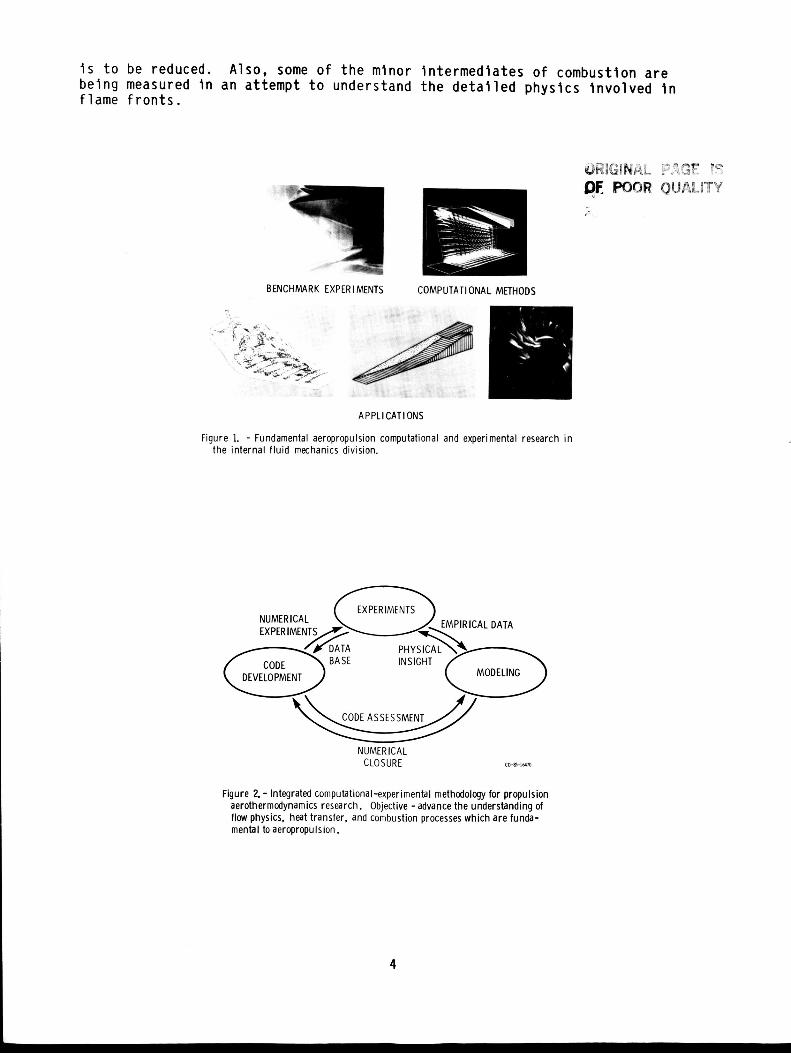
The goal of this research is to bring computational fluid dynamics to a
state of practical application for the aircraft engine industry. As shown in
figure 2, the approach is to have a strongly integrated computational and
experimental program for all the disciplines associated with the gas turbine
and other aeropropulslon systems by advancing the understanding of flow
physics, heat transfer, and combustion processes. The computational and
experimental research is integrated In the following way: the experiments that
are performed provide an emplrlcal data set so that physical models can be
formulated to describe the processes that are occurring - for example, turbu-
lence or chemical reaction. These experiments also form a data base for those
who are doing code development by providing experimental data against which
the codes can be verified and assessed. Models are generated as closure to
some of the numerical codes, and they also provide physical insight for exper-
iments. At the same time, codes which solve the complete Navler-Stokes
equations can be used as a kind of numerical experiment from which far more
extensive data can be obtained than ever could be obtained experimentally.
This could provide physical insight into the complex processes that are taking
place. These codes are also exercised against experimental data to assess theaccuracy and applicability of models (e.g., the turbulence model). We feel
that a fully integrated computatlonal-experlmental research program Is more
productive than other approaches and that It is the most desirable way of
pursuing our goal.
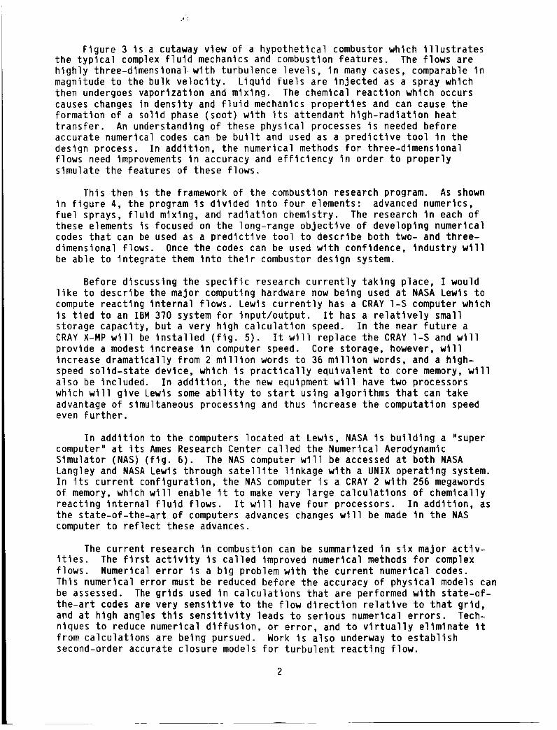
Figure 3 is a cutaway view of a hypothetical combustor which illustratesthe typical complex fluid mechanics and combustion features. The flows arehighly three-dlmenslonal with turbulence levels, in manycases, comparable inmagnitude to the bulk velocity. Liquid fuels are injected as a spray whichthen undergoes vaporization and mixing. The chemical reaction which occurscauses changes in density and fluid mechanics properties and can cause theformation of a solid phase (soot) with its attendant hlgh-radlatlon heattransfer. An understanding of these physical processes is needed beforeaccurate numerical codes can be built and used as a predictive tool in thedesign process. In addition, the numerical methods for three-dlmenslonalflows need improvements in accuracy and efficiency in order to properlysimulate the features of these flows.
This then is the framework of the combustion research program. As shown
in figure 4, the program is divided into four elements: advanced numerics,
fuel sprays, fluid mixing, and radiation chemistry. The research in each of
these elements is focused on the long-range objective of developing numericalcodes that can be used as a predictive tool to describe both two- and three-
dimensional flows. Once the codes can be used with confidence, industry will
be able to integrate them into their combustor design system.
Before discussing the specific research currently taking place, I would
like to describe the major computing hardware now being used at NASA Lewis to
compute reacting internal flows. Lewis currently has a CRAY 1-S computer which
is tied to an IBM 370 system for Input/output. It has a relatively small
storage capacity, but a very hlgh calculation speed. In the near future a
CRAY X-MP will be installed (fig. 5). It will replace the CRAY l-S and will
provide a modest increase in computer speed. Core storage, however, will
increase dramatically from 2 million words to 36 million words, and a high-
speed solld-state device, which is practically equivalent to core memory, will
also be included. In addition, the new equipment will have two processors
which will give Lewis some ability to start using algorithms that can take
advantage of simultaneous processing and thus increase the computation speedeven further.
In addition to the computers located at Lewis, NASA is building a "super
computer" at its Ames Research Center called the Numerical Aerodynamic
Simulator (NAS) (fig. 6). The NAS computer will be accessed at both NASA
Langley and NASA Lewis through satellite linkage with a UNIX operating system.In its current configuration, the NAS computer is a CRAY 2 with 256 megawords
of memory, which will enable it to make very large calculations of chemically
reacting internal fluid flows. It will have four processors. In addition, as
the state-of-the-art of computers advances changes will be made in the NAS
computer to reflect these advances.
The current research in combustion can be summarized in six major activ-
ities. The first actlvlty is called improved numerical methods for complex
I IUW_. IIUIII_I Ibal _l I Ul I_ a UI_ _1UUI_III WILII LII_ bU! I_IIL IIUIII_I I_OI _UU_3.
This numerical error must be reduced before the accuracy of physical models canbe assessed. The grids used in calculations that are performed with state-of-the-art codes are very sensitive to the flow direction relative to that grid,and at high angles this sensitivity leads to serious numerical errors. Tech-niques to reduce numerical diffusion, or error, and to virtually eliminate itfrom calculations are being pursued. Work is also underway to establishsecond-order accurate closure models for turbulent reacting flow.

The second activity Involves the development of techniques for makingpredictive calculations of chemically reacting flow. One of the more promisingtechniques, which is really In tts infancy, is called direct numerical slmu-latlons, or DNS. In this technique, the Navler-Stokes equations are solveddlrectly without any modeling of the turbulence. This technique is currentlybeing applied to reacting shear layers. Although this Is a relatively simpleflow, there is nevertheless a lo± of complexity associated with it. Much workremains to be done with this technique, but the results to date have been verypromising.
Another technique that has been used In several kinds of flows Is called
the random vortex method. This technique accounts for the vortlclty generated
at the wall of the confined flow and solves the vortlclty equation without any
turbulence closure modeling. Calculated results of flow over a rearward
facing step show many of the characteristics seen In hlgh-speed movies of
turbulent reacting flow experiments.
The third activity involves benchmark experiments for code development and
verification. Two-phase flow research Is currently underway. Detailed data
are required for code assessment, and instruments which Lewis has helped to
develop now show much promise of being able to make the appropriate measure-ments. (Those instruments are also being used to support icing research.)
Research is also being conducted on numerical calculation of two-phase flow.
Wlth the data from the experiments, an assessment of the current code capa-
bility wlll be made to guide future code development efforts. In addition, anextensive set of experiments is being conducted to look at the mixing of
dilution Jets into a cross stream in a channel. A substantial range of para-metric variables has been studied, and a Very complete set of data has been
established.
The next activity Is computer code applications. Currently available
codes are applied to real systems. The study of flow In the transition sec-
tion of a reverse flow combustor is an example of such work. Here a flow In
which fuel has already been burned has to undergo a 180 ° annular turn. Very
strong secondary flows arise, and the analysis Is very complex. Another
example Is the application of the Lewls-developed general chemical kinetics
programs and chemical equilibrium codes to problems of practical interest.
These codes are used throughout the world.
The next activity Is code development for thermochemlcal properties andklnetlc rates. Thermodynamic calculations for real gases are being performed
In support of future combustion models. The modeling of chemical kinetic com-
putations for complex reactions Is also being actively developed In support of
future computer codes.
The final activity In the current combustion research program Is to
advance the understanding of chemical mechanisms In reacting flow. Chemical
kinetic rates are measured using a shock tube facility. The data from thls
experiment are used to assess the kinetic models for various fuels of interest
In aeropropulslon systems. Detailed characteristics of one- and two-dlmen-sional controlled flames are also being established. We are interested in
studying the behavior of some of the minor species of flames and In looking atthe soot nucleation growth and eventual soot consumption in flames. Radiationheat transfer Is dominant In combustors and other aeropropulslon systems. The
control of soot nucleation and growth is essential if radiation heat transfer
3
is to be reduced. being measured in an attempt to understand the detailed physics involved in flame fronts.
Also, some of the minor intermediates o f combustion are
BENCHMARK EXPERl MENTS COMPUTATIONAL METHODS
A PPL I CAT I ONS
Figure 1. - Fundamental aeropropulsion computational and experimental research in the internal f luid mechanics division.
EXPERIMENTS NUMERICAL
MODELING INSIGHT
DEVELOPMENT
NUMERICAL CLOSURE CD-5-IMI
Figure 2. - Integrated computational-experimental methodology for propulsion aerothermodynamics research. Objective - advance the understanding of flow physics. heat transfer, and combustion processes which a r e funda- mental to aeropropulsion.
4

COMPRESSOR
EXIT AND _\
DIFFUSER-, !:_;:>" it- HIGH SWIRL AIR......./ _- __" , f ,
_" ... '_,'_ ,_ _,} __:_,.-DILUTION AIR JET
", I COMBUSTOR
AIR/REACTANT ., 'E._,,.;_,_ ..,;._,.Z_/_ ....
RECIRCULATION -" --" " _ ^i["srr__'''"
FILM COOLING AIR-"
CS_1478
Figure 3. - Illustration of the typical flow phenomena in a gas turbine combustor.
Typical flow is fully three-dimensional, has high turbulence levels, has chem-ical reactions and heat release, and occurs in two phases with vaporization.
RESEARCH LONG RANGE APPLICATION
ELEMENTS RESEARCH OBJECTIVES BY INDUSTRY
I ADVANCED h
NUMERICS
FUEL
SPRAYS
FLUIDMIXING
I RADIATION,CHEMISTRY
/
NUMERICAL CODES: _I COMBUSTORIPREDICT 2-D, 3-D | DESIGN I
REACTING VISCOUS V--I SYSTEM lINTERNALFLOWFIELDS
C.$851479
Figure 4. - Fundamental combustion research plan.
5

CYCLE TIME
STORAGE
PROCESSORS
ORIG3NBL PAGE IS O f POOR QUALITY
CRAY 1-5 (PRESENT)
12.5 nsec
2 x 10⁶ WORDS
1
CRAY X-MP (NOV. 85)
9.5 nsec
4x10⁶ WORDS CORE 32x 106 WORDS SSD
2
Figure 5. - Comparison of Cray 1-S and Cray X-MP computer capabilities.
NUMERICAL AERODYNAMIC SIMULATION
CRAY 2 with 256 mega words memory 250 mega flops with 4 CPUs UNlX operatinq system Remote user access -
Figure 6. - Numerical aeroaynamic simulator (NAS) computer capabilities and Lewis remote workstation.
6
N87-20269NUMERICAL STUDY OF COMBUSTION PROCESSES IN AFTERBURNERS
Zhou XlaoqlngChinese Aeronautical Establishment
BelJlng, People's Republic of China
and
Zhang XlaochunShenyang Aeroenglne Research Institute
Shenyang, People's Republic of China
Mathematical models and numerical methods are presented for computer
modeling of aeroenglne afterburners. A computer code GEMCHIP is described
briefly. The algorithms SIMPLER, for gas flow predictions, and DROPLET, for
droplet flow calculations, are incorporated in this code. The block correction
technique is adopted to facilitate convergence. The method of handlingirregular shapes of combustors and flameholders is described. The predicted
results for a Iow-bypass-ratlo turbofan afterburner in the cases of gaseous
combustion and multlphase spray combustion are provided and analyzed, and
engineering guides for afterburner optimization are presented.
INTRODUCTION
Thus far the design and development of alr-breathlng engine combustorshave been based mainly on ad hoc tests. But the past lO years have seen a
boom of numerical fluid mechanics and combustion. The computer modeling tech-
nique is beginning to establish itself in territory which has been dominated
exclusively by the empirical technique. It is believed that the combination
of numerical modeling with the seml-emplrlcal method and the modern diagnostic
technology will greatly promote combustion study and combustor design and
development.
The objective of this paper (which is part of the authors' continuing
effort to make computer models of multlphase turbulent combustion processes incombustors and furnaces (refs. 1 and 2 and private communication with X. Zhang
and H.H. Chlu, University of Illinois at Chlcago, 1984)) is to present mathe-
matical models and numerical methods for combustor flows and to apply these
methods to the computer prediction of aeroenglne afterburner characteristics.
The long-ignored droplet-turbulent-dlffuslon model plays an important role
in droplet dispersion and species distribution. It has now been incorporated
in this modeling. The K-c turbulence model is modified and extended to account
for multlphase turbulence effects. A hybrid, finlte-rate chemlcal-reaction
model based on a global Arrhenlus law and a turbulent mlxlng-rate model is used
Judiciously to predict the combustion rate of multlphase premlxed turbulent
flames. A system of conservation equations of the Eulerlan type is used forboth gaseous flow and multlslzed droplet flow predictions. To solve these
equations, the authors developed a computer code called GEMCHIP (general,
elllptlc-type, multlphase, combustion-heat-transfer, and Interdlffuslonprogram), in which the SIMPLER algorithm (ref. 3) for gaseous flow prediction

and the DROPLET(private communication with X. Zhouand H.H. Chlu, Universityof Illinois at Chicago, IgB3) procedure for droplet flow calculation wereincorporated. The block correction technique and the alternatlng-dlrectlonreclprocatlng-sweep llne-by-llne TDMA(trl-dlagonal matrix algorithm) methodwas adopted to facilitate convergence of the iteration processes.
The afterburner under study is a Iow-bypass-ratlo turbofan engine augmen-tor of the axlsymmetrlc type with a bluff body flameholder. The method of
simulating the irregularly shaped flow domain and the flameholder configuration
is described briefly and the inlet and boundary conditions are presented. The
usual wall functions (ref. 4) are used to bridge the near wall regions where
local Reynolds numbers are very low.
The numerical results of gas flow, droplet flow fields, and the spray
flame structures are presented. A study of the parametric sensitivity of thecombustion efficiency is made for both gas combustion and multlphase combus-
tion. Engineering guides are given for afterburner design optimization.
SYMBOLS
Cp specific heat of gas at constant pressure
E activation energy
h total enthalpy
J work-heat equivalence
K turbulent kinetic energy
L latent heat of vaporization
P gas pressure
q heat value of fuel
Ru universal gas constant
r_ droplet radius
T temperature
U,V velocities in X and R directions, respectively
W molecular weight
Y species mass concentration
r gamma function; transport coefficient
y stolchlometrlc coefficient

k
p
turbulence dlsslpatlon rate
heat conductivity
viscosity
density
mixture fraction
Nondlmenslonal numbers:
D1
Ec
Eu
Gc
Gd
Gv
Lmk
Nu
Pe
Pr
Re
Sc
_TR
CR
o
Subscripts:
b
eff
F
g
k
first Damkohler number
Eckert number
Eulerlan number
spray group combustion number
spray group aerodynamic drag number
spray group droplet preheating number
mass fraction of liquid In the mixture
Nusselt number
Peclet number
Prandtl number
Reynolds number
Schmldt number
ratio of flow residence tlme to turbulence dissipation tlme
ratio of turbulent kinetic energy to mean flow value
turbulent Schmldt/Prandtl number
boiling point
effective
fuel
gas
Kth slze group of droplets
liquid
9

M,m
o
ox
P
T,t
mean
initial or inlet condition
oxygen
product
turbulent; temperature
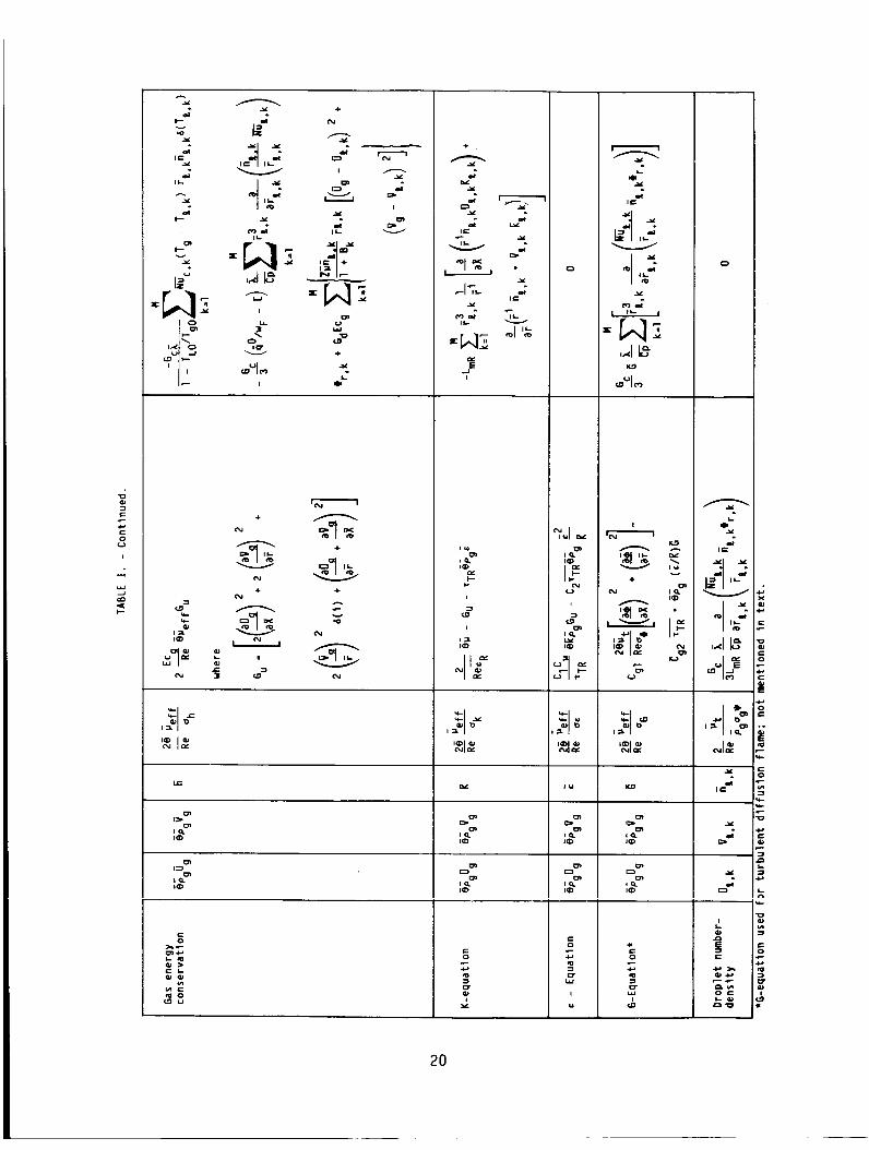
MATHEMATICAL FORMULATION
The Eulerlan scheme is used to construct elllptlc-type conservation
equations for both gaseous and droplet phases in two-dlmenslonal, multlphase,
combustlng, turbulent flows. Nondlmenslonallzatlon of these equations leadsto the following two general forms (ref. l and private communication with X.
Zhou and H.H. Chlu, University of Illinois at Chicago, 1983):
+a I FIr_ -- _r _ - r_ = S_ +aX aF aF Slnt
(i)
l[a_ (Fi_x_)+ a--ar(Fl_r_)] - LI_XFI Fl_x) a Fl_r]FI - ( + -- ( ) =Sln taF(2)
where Tx and Tr are fluxes in the X and R directions, respectively; r
is the transport coefficient for the variable K, S_ and Sln t are the _nner-phase and interphase source terms, respectively, ana i takes the values I = lfor the cylindrical coordinate and I = 0 for the Cartesian coordinate.
All conservation equations in these two forms are summarized in tables I
and II, respectively.
The physical models employed or developed In this study are introducedin the following sections.
Spray Spectrum Model
The generalized Rosln-Rammler function is adopted to derive the sizederivative of the droplet number density:
fn,_
n,S r [(t ÷ 4)/S] (t+l)/3 _r_ I Irr_____ Frr(t + 4)/s]IS/31
r_,m , [(t + I)/S] (t+4)/3" \riL,mJ exp I-\ ,ml L'Irr L'"+ i_i_II,.__ji (3)l
rg.,k+l/2n_, k = fn,_dr_ (4)
Jr_,k_I/2
lO

where S and t characterize the spray spectrum quallty, r denotes gammafunction, and nE and rE m are the droplet number density and the volume-mean initial droplet radlu_.
DROPLET Turbulent Diffusion Model
Besides the trajectory motion, droplets also disperse through diffusion
caused by the gas turbulence. A droplet diffusion model Is formulated (private
communication wlth X. Zhou and H.H. Chlu, University of Illinois at Chicago,
1983 and ref. 5) which takes the following final forms:
OnE = _ag (5)
I c 1= +_-_ _hj _4 K -r (6)
J \Pg
_T,_, = - VnE (7)
nEVg pgOg
_Tn,_, = - vnt (B)
E-_ Pg°nE
where oq and OnE are the gas and droplet turbulent Schmldt numbers,respectl_ely.
Modified K-c Model
The original K-c turbulence model is modified to take account ofdroplet-phase effects. The droplets are assumed to share turbulent kinetic
energy wlth the gas phase. The relationship of turbulent kinetic energies
between gas and droplets can be approximated as
KE ~ K/_ 2
The modified K-equation Is expressed as
Opg_gK) (0 _ef-----_f K)°K F'EKE_EdmpV • ( = V • V + BGk - Opg¢ - V "'0
The c-equation remains unchanged.
(9)
II

Hybrid Turbulent Gas Combustion Model
The combustion reaction is supposed to take place in a single step:
yF F + Yox 0 _ ypP (lO)
A hybrid combustion model is adopted; it assumes that the combustion rateis controlled by the slower of two competitive rates of successive subprocesses -
the chemical reaction rate and the turbulent mixing rate. The former rate is
determined by the Arrhenlus law, the latter rate is calculated from the eddy-
break-up (EBU) model
RF =- mlR_RF,EBU., .RF,Ar _ (ll)
where
:+i
_2
RF,Ar = -BaTgpgYFYox exp (-E/RuTg)
NUMERICAL METHODS
A 42 by 38 staggered grid system is superimposed on the flow domain. The
previously mentioned two general forms of nonlinear partial differential equa-
tions are then dlscretlzed into their finite difference counterparts by using
the control volume scheme and the primitive variables of pressure and velocity.
The power law scheme (ref. 3) is adopted to determine combined diffusion/
convection fluxes. The SIMPLER procedure is employed to predict gaseous flow
fields, it reduces computer time by 30 to 50 percent in comparison with the
popular SIMPLE procedure. The DROPLET procedure is used for calculating drop-
let flow fields. The alternatlng-directlon double-reclprocatlng-sweep llne-
by-line TDMA method is adopted to solve simultaneous algebraic equations Iter-
atlvely. The block correction technique is used to facilitate convergence.
The usual wall function method is employed to bridge the near wall regions
where the laminar viscosity effect is quite strong. This method is very effec-
tive in greatly reducing computer time while obtaining rather satisfactory
results. All these methods have been assembled into the computer code GEMCHIP.
The main flow chart of GEMCHIP is shown in figure I.
A droplet-free solution is first obtained through SIMPLER, which provides
both final results for the single gas-phase flow and the initial guesses of the
gas flow fields for muitiphase flow. Then we enter DROPLET to calculate drop-
let flow fields and the Interphase exchanges of mass, momentum, and energy.These quantities are substituted as source terms into SIMPLER, and the gas flow
fields are modified. Then we enter DROPLET again. This alternating Iteratlve
process continues until all the gas- and droplet-flow equations satisfy the
convergence criterion in all grids. The typical iteration number ranges from
40 to 75 for gas-phase burning problems and from 120 to 150 for multlphase
burning problems. The corresponding computer times are about 5 and 30 mln,respectively, on an IBM 4342 machine.
12
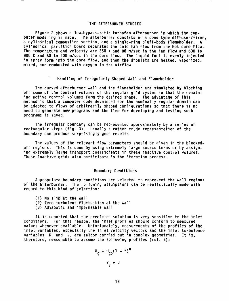
THE AFTERBURNER STUDIED
Figure 2 shows a Iow-bypass-ratlo turbofan afterburner In which the com-
puter modeling is made. The afterburner consists of a cone-type dlffuser/mIxer,
a cylindrical combustion section, and a slngle-rlng bluff-body flameholder. Acylindrical partition board separates the cold fan flow from the hot core flow.
The temperature and velocity are 350 K and BO m/sec in the fan flow and 600 to
800 K and 60 to 200 m/sec In the core flow. The liquid fuel Is evenly In_ectedin spray form into the core flow, and then the droplets are heated, vaporized,
mixed, and combusted with oxygen in the airflow.
Handling of Irregularly Shaped Wall and Flameholder
The curved afterburner wall and the flameholder are simulated by blocking
off some of the control volumes of the regular grld system so that the remain-
ing active control volumes form the desired shape. The advantage of thlsmethod is that a computer code developed for the nominally regular domain can
be adapted to flows of arbitrarily shaped configurations so that there is no
need to generate new programs and the time for developing and testing such
programs is saved.
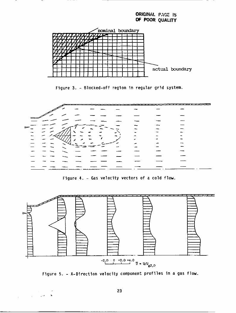
The irregular boundary can be represented approximately by a series of
rectangular steps (fig. 3). Usually a rather crude representation of the
boundary can produce surprisingly good results.
The values of the relevant flow parameters should be given in the blocked-
off regions. This is done by using extremely large source terms or by assign-
ing extremely large transport coefficients in these inactive control volumes.
These inactive grids also participate in the iteration process.
Boundary Conditions
Appropriate boundary conditions are selected to represent the wall regions
of the afterburner. The following assumptions can be realistically made withregard to this kind of selection:
(1) No sllp at the wall
(2) Zero turbulent fluctuation at the wall
(3) Adiabatic and impermeable wall
It is reported that the predicted solution Is very sensitive to the inlet
conditions. For this reason, the inlet profiles should conform to measured
values whenever available. Unfortunately, measurements of the profiles of the
inlet variables, especially the inlet velocity vectors and the inlet turbulence
variables K and c, are seldom carried out in complex geometries. It is,therefore, reasonable to assume the following profiles (ref. 6):
Ug = Ugo(1 - F)n
V =0g
13
c = co (K/Ko)1.5
where 0.2 > n > 0 and 2 > m > O. The variables with subscript o denotevalues at the centers of cote fTow or fan flow. The nondlmenslonal radiusT = r/R for the core flow and T = Ir - (Rl + Ro)/21/((R1 + Ro)/2) for the fan
flow, where Ro denotes the radius of the partition board and Rl representsthe diffuser's inlet radius.
The inlet profiles of the droplet number densities, temperatures, and
velocities vary wlth the fuel nozzle type and spray quality.
In the axis of symmetry the radial gradients of all droplet-phase vari-
ables are taken to be equal to zero.
The exit plane should be located far downstream and outside the reclrcula-
tlon zone so that the local parabolic flow assumption applies and that the
calculating domain is isolated from the ambient environment. The only excep-
tions are the equations for pressure p and for the pressure correction param-
eter p', since the pressure effect is always two way. The problem is solved
by calculating the outlet velocity component in the main flow direction.
RESULTS AND DISCUSSIONS
The objectives of the numerical study are to analyze the shape and thesize of reclrculatlon zones at different working conditions, to examine the
vaporization process of multlslze fuel sprays, to compare the multlphase flame
structures with the gas flame structures, and to study the parametric sensitiv-
ity of afterburnlng efficiency.
Reclrculation Zones
The gas velocity vector fields inside the afterburner are shown infigures 4 to 6 for gas flow and multlphase flow. The numerical calculationsreveal that the reclrculatlon zones in the wake of the flameholder are induced
by negative pressure gradients, which, in turn, are caused by gaseous viscosity.
Figures 4 and 5 are pictures of velocity vectors and X-dlrectlon velocity
component profiles in a gas phase flow. The length of the reclrculatlon zonein the cold flow case is about 2.0 to 3.5 times the flameholder width. It Is
readily seen from figure 4 and 5 that the wake effect still exists far down-
stream of the flameholder. Some experimental reports claim that the reclrcula-
tlon zone wlll uuLu,,_ larger and longer In gas combustlu,, _ases u=_=u_: of gas
expansion and the reduction of the absolute value of the negative pressurebehind the flameholder. But this trend is not obvious in this calculation.
Research work is under way in thls direction.
Figure 7 shows droplet velocity vectors of two size groups in the multi-
phase afterburnlng condition. A comparison of the multlphase flow with the
gas flow field (fig. 6) shows that the small droplets are capable of reaching
14
velocity equilibrium more qutckly than the large droplets. The velocity non-equilibrium In the downstream Is somewhat enhanced because the gas is acceler-ated more rapldly than the droplets. This is especlally true for the largedroplets. The droplet reclrculatlon zone Is obviously smaller than the gasreclrculatton zone.
Cascading Vaporization
The preheating and vaporization processes of droplets of different slze
groups are illustrated In figure 8. It Is readily seen from the predicted
curves that the small droplets (e.g., D1 = 0.15) complete the preheating
process and initiate the vaporization process much earlier than the large
droplets (e.g., Dl = 1.60).
The phenomenon of successive initiation of the vaporization of droplets
of different sizes In spray Is designated as cascading vaporization (ref. l)
since the initial vaporization lines of different slze droplets constitute aform of cascade.
Gas Flame and Multlphase Flame Structures
Figures g(a) and (b) show the temperature field and flame structure ofthe gas combustion flow. The gas flame structure Is rather simple: the flow
of the combustible mixture mixes wlth the fan flow of the cold alr, and theflame Is stabilized In the reclrculatlon zone close behind the flameholder.
There Is a "dark" area, which Is fuel-deflclent, In the wake of the flame-
holder. Thls Is where the combustion Is completed.
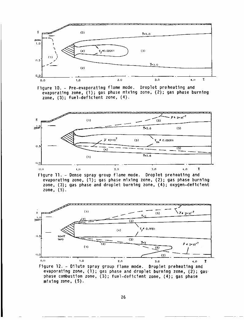
The structure of the multlphase flame Is very complicated. Calculation
reveals that there are three principal combustion modes: (1) pre-evaporatlng
flame, (2) dense spray group flame, and (3) dilute spray group flame. The
total fuel-alr ratio and the spray group combustion number Gc are the two
maln parameters determining combustion mode. The Gc Is actually the ratio
of the characteristic vaporization rate to the convection flow rate and was
first proposed by Prof. H.H. Chlu (ref. 7).
Pre-evaporatlng flame. - The pre-evaporatlon flame Is shown In figure lO.
When the Gc number Is very large (fine atomization, i.e., the spray con-sists of an extremely large quantity of small droplets) all the droplets are
vaporized at a typical afterburner inlet temperature before they get to the
flame zone. The flame structure Is similar to that of gas phase combustion.
Dense spray qroup flame. - If the Gc number Is rather large and thefuel-air ratio Is also high, dense spray group combustion occurs (fig. ll);
thls Is characterized by the presence of an oxygen-deflclent zone, which
decreases combustion efficiency. Both types of gas and droplet burning coexistin the flame.
Dilute spray qroup flame. - Thls,mode occurs at a small Gc number, whichIs characterized by poor atomization quality and a low fuel-alr ratio: that
Is, there Is a small quantity of blg droplets. If the droplet slze Is large
enough and droplets concentrate near the central llne of the afterburner, the
v-type flame shown In figure 12 may appear. Thls type of flame Is unstable.
15
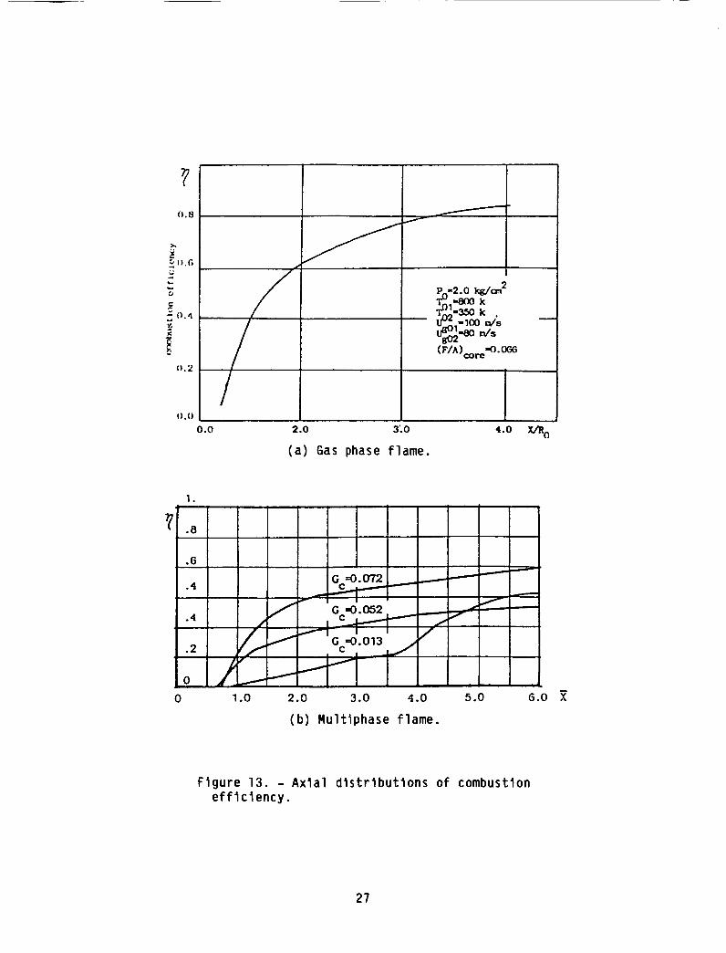
Figures 13(a) and (b) show, respectively, the axial distributions ofafterburnlng efflclencles in gas-phase and multlphase combustion cases. It isseen that the growth of the combustion efficiency for the multlphase flame hasa slower start than that for the gas flame. This difference is caused by thedroplet preheating and by vaporization processes. The results also indicatethat the smaller the spray group combustion number Gc, the larger thedifference.
Parametric Sensitivity Study of Combustion Efficiency
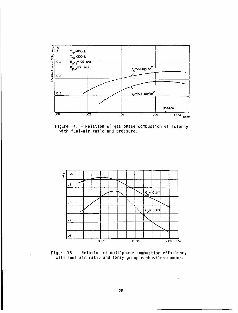
Figure 14 showsthe effect of fuel-alr ratio on gas-phase combustion effi-ciency at two different pressures (2.0 kg/cm2 and 0.5 kg/cm2). The effl-clency curve reaches its peak at an approximately stolchlometrlc fuel-alr ratioin the core flow. At higher pressures, the efficiency peak movestoward richerm_xtures and the curve becomesflatter because of the dilution action by thefan flow and the improvement of combustion conditions.
Figure 15 showsthe variation of the multlphase combustion efficiency withthe fuel-air ratio at two different spray group combustion numbers. Withmultlphase combustion there is a combustion efficiency peak at an appropriatefuel-alr ratio similar to that with gas-phase combustion. With an increase ofGc number, the efficiency peak movestoward leaner mixtures - which meansmixtures with a larger numberof smaller-slzed droplets will have a higher com-bustion efficiency at a lower fuel-alr ratio. The results are also in agree-ment with the experimental measurements.
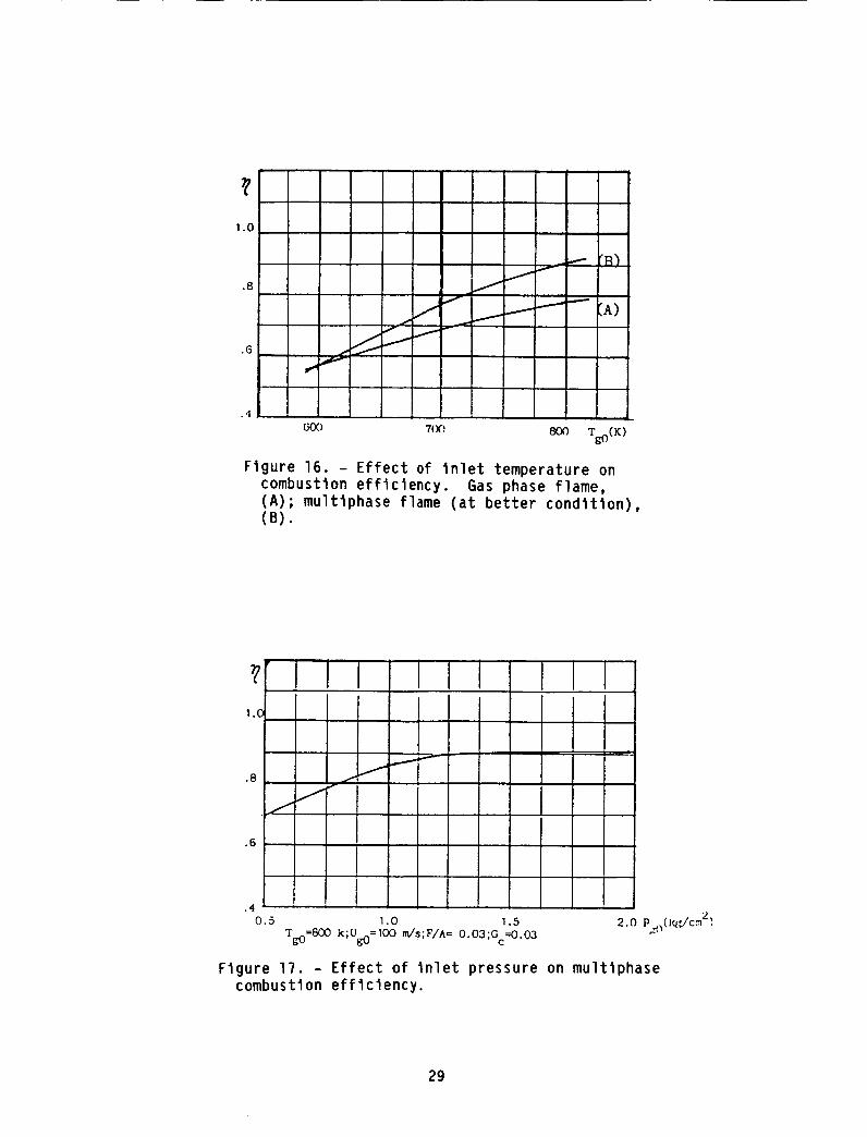
Figures 16(a) and (b) showthe effect of the inlet gas temperature on com-bustion efflclencles of gas-phase and multlphase flames. The temperatureincrease enhancesthe heat release rate and speeds up droplet vaporization,which, in turn, enhancesthe combustion efficlencles of both the gas and multi-phase flames. But, for obvious reasons, the temperature effect is stronger inmultlphase flames.
The effect of inlet gas pressure on combustion efficiency is similar to
that of inlet temperature. It is seen from figure 14 that, in the case of gas
phase combustion, an increase of gas pressure from 0.5 to 2.0 kg/cm 2 signifi-
cantly improves combustion. Figure 17 shows the increase of combustion
efficiency with gas pressure in a multiphase combustion case. The pressure
effect is negligible at pressures greater than 1.3 kg/cm 2.
Figure 18 shows the effect of gas-flow velocity on gas-phase combustion
efficiency. An increase in ga s velocity results in a decrease in combustion
efficiency because of the reduction of the residence time of the gas flow in
the afterburner. The higher the velocity, the lower the efficiency. The
effect of inlet gas velocity on multlphase combustion efficiency is rathercnmnllr_fpdr........................_Inr_ th_ v_Inri_y _,.__r÷_ nnt,,v_nlv,,,y÷h_,,__ac_anr_,_,_,,_ ÷_m_,,.,__h"_ alc_
the droplet atomization, vaporization, and spray group combustion number Gc.
CONCLUSIONS
The mathematical models and numerical methods for predicting multlphase
turbulent reacting flows, developed in the authors' study of spray group com-bustion phenomena have been successfully extended and applied to the numerical
16
study of flow fields and combustion characteristics of a low-bypass-ratioturbofan afterburner. The computer code developed by the authors Is versatileand effective In thls study. The technique of blocking off relevant controlvolumes makes It posslble for a computer code developed for a regular gridsystem to be applied to arbitrary flow domains.
The numerical analysls reveals that the size of the rectrculation zonebehind the flameholder is about 2.0 to 3.5 times Its width. The droplet reclr-culatlon zone Is smaller than the gas reclrculatton zone and decreases or evendisappears with an increase In droplet size.
The calculation also exposes the existence of three principal combustionmodes In multlphase combustion. They are the pre-evaporatlng flame mode, thedense spray group flame mode, and the dilute spray group flame mode. Study offlame structure Is useful to afterburner design optimization.
The results reveal the dependence of afterburner combustion efficiency onthe fuel-alr ratio and on the operating parameters (such as the Inlet gas tem-perature, pressure, and velocity). As for multlphase combustion, whichprevails in turbofan afterburners, the spray group combustion number has asignificant effect on combustion efficiency and flame structure. It Is con-cluded that afterburners should be designed to work In the optimum spray groupcombustion number, which is related to the fuel-air ratio and Its distribution.Generally speaking, the favorable design has a pre-evaporatlng flame mode or adense group combustion mode with an Initial fuel distribution capable of keep-lng oxygen-deflclent zones as small as possible.
Although the previously predicted results are In good qualitative agree-ment with the known facts, accurate dlagnostlc measurements and detailedexperimental verifications are necessary to examine the quantitative agreementand to improve the present models.
•
o
,
,
,
REFERENCES
Chlu, H.H.; and Zhou, Xlaoqlng: Turbulent Spray Group Evaporation and
Combustion, 9th International Colloquium on Dynamics of Explosion and
Reactive System, Polter, France, 1983.
Zhou, Xlaoqlng; and Chlu, H.H.: Spray Group Combustion Processes In Alr
Breathing Propulsion Combustors, AIAA-83-1323, AIAA/ASME/SAE 19th Joint
Propulsion Conference, 1983, Seattle, U.S.A.
Patankar, S.V.: Numerical Heat Transfer and Fluid Flow, McGraw-Hlll,
1980, U.S.A.
Launder, B.E.; and Spalding, D.B.: The Numerical Computation of Turbulent
Flows, Computer Method In Applied Mechanics and Engineering, Vol. 3,
pp. 269-289, 1974.
Ward, P.; Colllngs, N.; and Hay, N.: A Comparison of Simple Models of
Turbulent Droplet Diffusion Suitable for Use In Computations of SprayFlames, ASME-B2-WA/HT-2.
17

°
°
Khalil, E.E.: Numerical Computations of Turbulent Reacting CombustionFlows, Numerical Method in Heat Transfer, 1981, John Wiley and Sons Ltd.
Chlu, H.H.; and Llu, T.M.: Group Combustion of Liquid Droplets, Combus-
tion Science and Technology, 1977, Vol. 17, pp. 127-142.
18

v
zcp
w
o
z
=o
o_=
z
ciO
I=-
I
0_
i_i. sI"
e,
¢u
I--
fi.
I
o
o
..t
,..I I_
4"
(u
8
÷
I_l_
_l_
I
lID
I_l) I_
10 10
_=_
e,
I
i="
I
o
4-
IU
4.
,ol '_
,.-1"7,.
I
I
÷
_ I_
I I
IQ.
¢0
Co
_|
I
o_
v
i="i=_
¢.0
I
÷
CP
, i i
...II,..i.I,.i.'Ih
o
I
"T,-
o
÷
3
A
' ,-5----,
_ _ i_ I_
_ t_ '®
Os
I
.#I e,_1_,
,.,*I
o
_4D
4),
c
E _
lg
®
co
i
N
I
v
le/
h_ _
II
('_
,2 ,#
z[,,,1_
_ ,,.o
I
117
I
4.
÷
#
4-
&
I
,_ ÷
N _
÷
.
÷
_p
I%1
I
÷ •
-M_2#
i
I
I_IDI_ i_ I_
i_ _ iz::l I_
i
i-
I
,® _÷
e,,l_
i::1._
*2
,,,I k_
_ E
L
w
I w
c
,!
2O

ORiGt_r,L P,_G,_ IS
OF POOR OUALITY
I
v
A
i_1.,L-
i_c..x
A
I I!
, _1__ _1_
°
,=,,, ,=-, ,=,,,,
== ,?, |
°
II
N
N o
,:o
, o
r.,,.
ii
°
II
. II
ii #
°.
II
°°
NO
ii
_o
I1
ii
0°
o o
o
II
II
H
W I---°
o
_o
H
°.
AO
I
O
_J
_o1_N
°°
H
f
21

C start!
Set the problea i
i FI Nondl_cnsional I -zation
Grid & Guees J I SourCeterm
calculation,,
No Yes _ Key .= I I' Key'= 2
Print flow fleld
Key" I _ Key= 2
Interphaseand heat
ex_
C..°p _
Figure I. - Main flowchart of GEMCHIP.
I/ I z
Diffuser
_ l i / , , _ // t -" /i / • _ z / ; ,.. z / 1/
/
P_ =_'_holde r
Figure 2. - Afterburner studied.
22
ORIGINAL PAGF. IS
OF POOR QUALITY
nal boundary
actual boundary
Figure 3. - Blocked-off reglon in regular grid system.
f///,t " .... "-,
I
Figure 4. - Gas velocity vectors of a cold flow.
Figure 5. - X- Directi on
-2.0 0 +2.0 +4.0
L , ' ' U = U/Ug2, 0
velocity component profiles in a gas flow.
23

-_._ - _ ......
Figure 6. - Gas velocity vectors of a multiphase combustion flow.
151-o. i,_
"_ ,m" • P
DI-I .G
Figure 7. - Droplet velocity vectors of a multlphase combustion flow.
I / 1 TRG=_ X_ k
I I |R irm.)-().()40mm
NI-Z_XI 1Figure B. - Cascading vaporization of a multlphase spray flow.
24 ORIGINAL PAGE IS
POOR QUALITY

ORIGINAL PAGE IS
OF POOR OUALITY
J
I
(a) Temperature field In a gas combustion flow.
(b) Gas fuel concentration field In a gas phase combustion flow.
Figure 9. - Gas phase combustion flow.
25
1.0
(_.5"
0o0 ! i ,,- . I i
0.0 1.0 2.0 3.0 4.0 ._
Figure I0. - Pre-evaporatlng flame mode. Droplet preheatlng andevaporatlng zone, (I); gas phase mlxlng zone, (2); gas phase burnlngzone, (3); fuel-deflclent zone, (4).
0._
().()
I
(_)
%,3.6 (3)
(5)\
Y • 0.00001OX
(3)
_=3.6
().(J ! .() 2.0 3.0 4.0
Flgure 11. - Dense spray group flame mode. Droplet preheating andevaporating zone, (1); gas phase mlxlng zone, (2); gas phase burningzone, (3); gas phase and droplet burning zone, (4); oxygen-deflclentzone, (5).
. , . i x . ..................... . " " " "jr .... - - - -11) / (._)R .---'" _ _ 2" I0-7_....____.___
0.5
0.0
(3)
bZ____ C4)
body _ _ --..._.._ _ (3)(2)
(1)
\¥_ O.0001
/
_'3 3/ "_ 2* 10 "7
_ (5) _ I
! ! i
().() 1.0 2.0 3.0 4.0
Figure 12. - O11ute spray group flame mode. Droplet preheatlng andevaporatlng zone, (I); gas phase and droplet burnlng zone, (2); gas _phase combustlon zone, (3); fuel-deflclent zone, (4); gas phasemlxlng zone, (5).
26
?
0.8
e-
-- 0.4g
o.2
/
PO,,2.0 kg/a_ 2T 1_") k__=3,_ k .uU_L_-lOO=/s_._-80 rv's
2.0 3"0
(a) Gas phase flame.
4.o X/R o
?1,
.8
.6
l_=o.o72
.2 r/__ / .,.,,,,"_ G l
_0.013
o /1.0 2.0 3.0
f/
/
j/
4.0 5.0 6.0
(b) Rultlphase flame.
Figure 13. - Axlal distributions of combustlonefflclency.
27
(Jc-O
e-0
0.9
0.8
I
TO l'eO0 k
T02=350 k
UB01" 100 m/s
Ug02"_O m/s
:0.7 f
%=2. _cm 2
pn=,_. 5 kg/om 2
O0 .02 .04 .0(3 (F/A)cor c
Figure 14. - Relation of gas phase combustion efficiencywith fuel-alr ratio and pressure.
1.0
.9
.8
.7
J/
J
//
\"_ G = 0.07
_C
= 0.01G c
",,,,
.0
0 0.02 0.04 0.0(3 F/A
Figure 15. - Relation of multlphase combustion efficiencywith fuel-alr ratio and spray group combustion number.
28
.8
.6
.4
"_ jlfr
f
J
1 I--- IA)
@ 7{)0,800 T_3(K )
Figure 16. - Effect of Inlet temperature oncombustion efficiency. Gas phase flame,(A); multlphase flame (at better condition),(B).
.8
J
.6
.4
0.5
J
f
JJ
F
F
1.0 1.5
Tgo=800 k;Ugo=100 m,/s F/A= 0.03;Gc=0.03
2.0 P _(lq;/c,.'n2_,
Flgure 17. - Effect of lnlet pressure on multlphasecombustlon efflclency.
29

.9
.8
.?
.6.5(} IIGO l_=Xl U
I)1_1=11.5 I<l.d(nT; "rl,ii=H<Xl k; (I,'/A)=().(),'-'_,:)
(n/,_)
Figure 18. - Effect of inlet gas flow velocity on gascombustion efficiency.
30
N87-20270
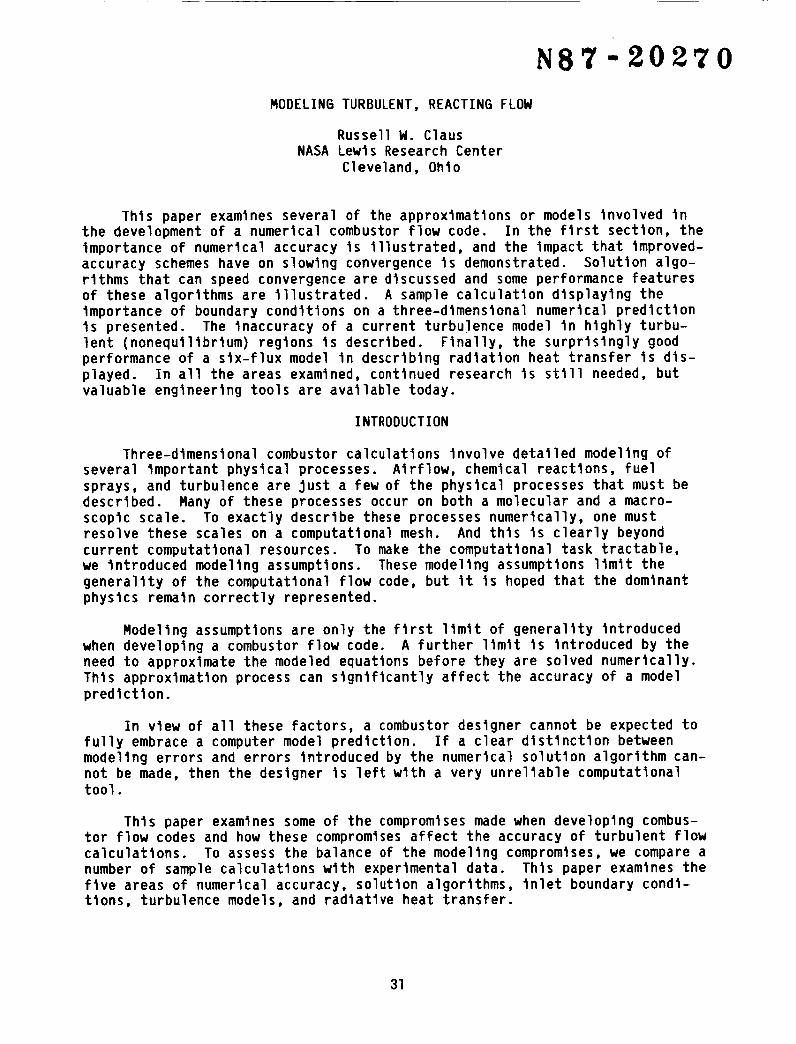
MODELING TURBULENT, REACTING FLOW
Russell W. ClausNASA Lewis Research Center
Cleveland, Ohio
This paper examines several of the approximations or models involved inthe development of a numerical combustor flow code. In the first section, the
importance of numerical accuracy is illustrated, and the impact that improved-
accuracy schemes have on slowing convergence is demonstrated. Solution algo-
rithms that can speed convergence are discussed and some performance features
of these algorithms are illustrated. A sample calculation displaying the
importance of boundary conditions on a three-dlmenslonal numerical prediction
is presented. The inaccuracy of a current turbu]ence model in highly turbu-
lent (nonequlllbrlum) regions is described. Finally, the surprisingly good
performance of a slx-flux model in descrlblng radiation heat transfer Is dls-
played. In all the areas examined, continued research is still needed, but
valuable engineering tools are available today.
INTRODUCTION
Three-dlmenslonal combustor calculatlons involve detailed modeling of
several important physical processes. Airflow, chemical reactions, fuel
sprays, and turbulence are Just a few of the physical processes that must be
described. Many of these processes occur on both a molecular and a macro-
scopic scale. To exactly describe these processes numerically, one must
resolve these scales on a computational mesh. And this is clearly beyond
current computational resources. To make the computational task tractable,we introduced modeling assumptions. These modeling assumptions limit the
generality of the computational flow code, but It Is hoped that the dominant
physics remain correctly represented.
Modeling assumptions are only the first limit of generality introduced
when developing a combustor flow code. A further limit Is introduced by the
need to approximate the modeled equations before they are solved numerically.
Thls approximation process can significantly affect the accuracy of a model
prediction.
In vlew of all these factors, a combustor designer cannot be expected to
fully embrace a computer model prediction. If a clear distinction between
modeling errors and errors introduced by the numerical solution algorithm can-
not be made, then the designer is left wlth a very unreliable computationaltool.
Thls paper examines some of the compromises made when developing combus-tor flow codes and how these compromises affect the accuracy of turbulent flow
calculations. To assess the balance of the modeling compromises, we compare a
number of sample calculations wlth experimental data. This paper examines theflve areas of numerical accuracy, solution algorithms, inlet boundary condi-
tions, turbulence models, and radiative heat transfer.
31

The NUMERICALACCURACYsection focuses on the development of more accu-rate numerical methods to be used In combustor flow codes. Upwind differenc-ing, which Is currently used in these flow codes, introduces an appreciableerror (or numerical diffusion) Into the calculation. This error may be ofsuch a large magnitude that It obscures the turbulence model used In the cal-culation. A series of calculations are illustrated which demonstrate theaccuracy of a variety of differencing schemes.
An important aspect of improved accuracy is the effect that the differ-encing scheme has on the rate of convergence. The improved accuracy schemesall appear to require more CPU tlme to converge. For this reason, the nextsection discusses solution algorithms. SIMPLE (semi-Implicit pressure-linkedequations) is one of the most widely used solution algorithms for solving thesteady-state form of the Navler-Stokes equations. Although this scheme hasproven to be quite effective, its convergence rate can be improved. Thispaper focuses on two approaches which accelerate convergence by performingcorrections that improve the lteratlve agreement with continuity. Thesealternate schemes are illustrated In a series of calculations.
A third section examines the importance of inlet boundary conditions. An
illustrative example Is displayed.
The fourth section discusses turbulence models and reaction closures.
Here the more pragmatic approaches to calculating turbulent reactions are
illustrated. An eddy-breakup model and a PDF (probability density function)
method are described and compared.
Finally, the fifth section examines the accuracy of a radiation heat-transfer model. A six-flux model of radiative heat transfer Is described.
This model provides only a limited geometric description of the radiation
transfer process, but a comparison wlth experimental data indicates an encour-
aging level of agreement.
NUMERICAL ACCURACY
The following Is a general form of the tlme-averaged equations that mustbe solved In a combustor flow code:
a_(pu_) a a a a__ (1)
where _ can represent U, V, W, UlUJ'dK'anc, or H; where r_ Is thediffusion coefficients (e.g., _eff); S_ Is the source term (e.g., - aP/ax).The equation represents convection of a conserved scalar that Is subtracted bydiffusion terms equal to a source term that could represent a pressure gradi-
ent or a source/slnk term. These equations are solved by dlscretlzlng on as÷...... _ ._h ,,_._ _h^ _= volu,,,_m=_huu i l) ,,_ _ayy_,_u ,,,_._u_ ................ _ .... flnl _ ...... _ ^_ t,'_ g. • _-, "_ ...... _ ....system Is used to avoid the pressure-veloclty decoupllng that can result In afinite volume representation of incompressible flow.
An example of the dlscretlzatlon of a convective term using central dlf-
ferencing Is the following:
32
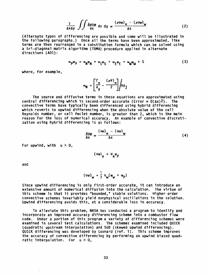
AxAy dx dy =(pU_) e - (pu_) w
&X(2)
(Alternate types of differencing are possible and some will be illustrated inthe following paragraphs.) Once all the terms have been approximated, llke
terms are then rearranged in a substitution formula which can be solved using
a trl-dlagonal matrix algorithm (TDMA) procedure applied in alternate
directions (ADI):
_p_p = =N_N + =S_S ÷ aE_ E + aW_ W + S (3)
where, for example,
rn (.V)n]/=N: 2
The source and diffusive terms in these equations are approximated using
central differencing which is second-order accurate (Error = O(Ax)2). The
convective terms have typically been differenced using hybrid dlfferenclng
which reverts to upwind differencing when the absolute value of the cell
Reynolds number, or cell Peclet number, is greater than 2, which is the main
reason for the loss of numerical accuracy. An example of convective dlscretl-
zatlon using hybrid differencing is as follows:
(U_)e - (u_)wax _ ax (4)
For upwind, with u > O,
(u_) e = Ue_ P
and
l(u_)w = _ Uw(_w + _,p)
Since upwind differencing is only flrst-order accurate, It can introduce anextensive amount of numerical diffusion into the calculation. The virtue of
this scheme is that it provides "bounded," stable solutions. Higher order
convective schemes invariably yield nonphysical oscillations in the solution.Upwind differencing avoids this, at a considerable loss in accuracy.
To alleviate this problem, NASA has conducted a program to identify and
incorporate an improved accuracy differencing scheme into a combustor flow
code. Under a portion of this program a variety of differencing schemes wereexamined in several test calculations. The schemes examined included QUICK
(quadratic upstream interpolation) and SUD (skewed upwind differencing).
QUICK differencing was developed by Leonard (ref. 1). This scheme improves
the accuracy of convective differencing by performing an upwind biased quad-
ratic interpolation. For u > O,
33

1 3 3 /(Urn) e = ue - _mw * _mp * _mE
_l 3 3p)(uq,)w = uw w
(S)
where grid point locations are as noted on figure 2. This scheme Is second-order accurate and can produce nonphysical oscillations tn the solution. SUO(skewed upwind differencing) (ref. 2) attains high accuracy by differencing inan upwind manner along the flow streamlines. Whtle maintaining the same for-mal accuracy as upwind differencing, the truncation error In SUO Is smaller.For example:
For u > 0 and V > O,
(u_)e = Uem P
(um)w = Uw(1 - _)m w + Uw=msw
V = minimum of (l,V/2u)
(6)
where grld point locations are as noted In figure 3. As wlth QUICK, SUD can
produce nonphysical oscillations in the solution; therefore, a scheme to"bound" SUD was also examined. This scheme employs the concept of flux-
blending (ref. 3), wherein a bounded flux determined from upwind differencing
Is blended wlth the unbounded, but more accurate, SUD flux. The maln factorIs to blend as little of the lesser accurate scheme while still maintaining a
properly "bounded" solution. Thls procedure, called BSUDS, starts from an
initial, totally skew-dlfferenced estimate and blends an upwind flux If the
solution Is out of the range of neighboring values. If the solution is In
range (i.e., bounded), then no blending Is performed.
An illustration of the accuracy of the upwind, QUICK, and SUD schemes Is
seen In figure 4. This figure displays the results of a slngle-polnt scalar-
transport calculation made for various flow angles. All schemes agree with an
exact solution (no error) at a zero flow angle; however, at angles greater
than zero, each scheme displays some degree of error relating to numerical
diffusion. The error displayed by upwind differencing increases wlth flow
angle to a maximum at 45°. The QUICK scheme displays a similar behavior, butthe overall error Is much less. The SUD scheme displays a maximum error
around 15°, but It tends to zero at angles approaching 45° Both QUICK andSUD display a much higher level of accuracy than upwind.
Although a scalar transport calculation Is useful for a general examina-tion of some aspects of differencing scheme performance, a laminar flow calcu-
lation Is a more complete test. The results of a series of laminar flow
calculations from reference 4 are displayed In figure 5. In thls figure,axial velocity profiies at a distance of one-half a duct height from the _nlet
are shown for two different computational meshes. In these calculations, thesteepness of the velocity profile indicates accuracy. Steep velocity profiles
are exhibited by QUICK and BSUDS; the upwind profiles exhibit a hlgh degree of
numerical diffusion. On the coarse mesh, BSUDS appears to be more accuratethan QUICK; on the flne mesh, there Is not much of a distinction between thetwo schemes.
34

An important aspect of improved accuracy Is the effect that the differ-enclng scheme has on the rate of convergence. The computational times toconverge the system of governing equations In the previous laminar calcula-tions are shown tn table I. The convergence times are ratioed to the upwindconvergence times to clearly illustrate the computational penalty paid toattain improved accuracy. Generally, the improved accuracy schemes requiredfrom 3 to 15 times longer to reach a converged solution. To a degree one canhope that this computational penalty can be offset by using coarse meshes toachieve the same overall level of accuracy. In reality, a relatively finemesh Is needed, even with the high-accuracy schemes. In any case, the needfor improved solution algorithms for these more accurate differencing schemesIs strongly indicated.
SOLUTION ALGORITHMS
The previous section demonstrated the need for improved solution algo-rithms. Thls section examines the widely used SIMPLE algorithm and two modi-fications to this scheme. These schemes cover only a small portion of the
wlde range of methods to accelerate solution convergence. Vectorlzatlon,dlrect-solutlon methods, and multlgrld methods - to llst Just a few - are allareas of active research that are certain to yield much greater computational
benefits In the near future.
In the SIMPLE algorithm, a guessed pressure field is inserted Into the
dlscretlzed momentum equations to obtain a velocity field. The pressure field
is corrected by an equation which Is derived through a combination of the con-tinuity and momentum equations. The velocity field Is then updated and is
used In the solution of the equations for k, c, and _. The corrected pres-
sure field Is treated as the guessed pressure field, and the procedure Is
repeated until a converged solution Is obtained.
for
The following velocity correction equation is used In the SIMPLE scheme
u at point e:
n_b AnbUnb + (P_ - P_)A eAeU'e =
Primes indicate corrections to old values. The underlined term, which repre-
sents the influence of corrected pressures on neighboring velocities, is
neglected In the SIMPLE algorithm. The converged solution Is unchanged by theexclusion of thls term slnce, for the steady-state solution, the corrections
go to zero. Neglecting terms, however, does force the use of low underrelaxa-
tlon factors, which can slow convergence.
The SIMPLER algorithm improves on the SIMPLE scheme by including the
previously neglected terms when calculating the pressure field. The calcula-tion sequence starts wlth a guessed velocity field. An equation that solves
for the pressure field (using the terms ignored In the SIMPLE scheme) Is cal-culated from the guessed velocity field. Thls pressure field is then used tosolve the dlscretlzed momentum equations to obtain a velocity field. The
velocity field Is corrected In a manner similar to the SIMPLE velocity correc-
tion. Thls velocity field Is then treated as the guessed velocity field, and
the iteration procedure is repeated until convergence Is reached.
35

Because additional equations are solved, each iteration through the
SIMPLER routine involves more computational time than an iteration step throughSIMPLE. However, higher underrelaxatlon factors can be applied in the SIMPLER
routine, thereby accelerating convergence.
The PISO scheme also takes into account the terms neglected in the SIMPLE
code, but in a different manner. The PISO routine mimics the SIMPLE approach
until the end of the first iteration. At this point, the PISO scheme employsan equation containing the neglected terms to correct the pressure and veloc-
Ity field to more closely agree with continuity. Again, this procedure is
repeated until the solution converges. In this manner, the PISO code allows
for higher underrelaxation factors to accelerate convergence.
The performance of these various solution schemes is displayed in
figure 6. As an example, the convergence times for a 38-by-38 grid point
calculation are plotted as a function of underrelaxation factor (fig. 6(a)).When a reasonably large underrelaxatlon factor is used, SIMPLER or PISO con-
verge about twice as fast as SIMPLE. In addition, SIMPLER and PISO converge
over a larger range of underrelaxatlon factors than SIMPLE. From an engineer-ing standpoint, improving the "robustness" of a computational scheme is often
Just as important as accelerating convergence. The computational benefit of
using SIMPLER and PISO for flne-mesh calculations is displayed in figure 6(b).The greater the number of mesh points used in the calculation, the greater the
benefit of SIMPLER or PISO over SIMPLE. For example, a calculation of approx-imately 3300 grid points converges three times faster using PISO or SIMPLER
than it does using SIMPLE. This is a savings of about 600 CPU seconds. The
1440 grid points calculation demonstrated a savings of only about lO0 CPUseconds.
INLET BOUNDARY CONDITIONS
In any calculation of a complex, three-dlmenslonal turbulent flow, the
boundary conditions that are needed in the calculation are frequently unknown
or unmeasured. The use of inappropriate values at the computational boundarycan sometimes be the main limit to the calculatlon's predictive capability.
This error can sometimes be more important than numerical accuracy or turbu-lence model considerations. Figure 7 shows an example of a three-dlmenslonal
Jet-ln-crossflow calculation using alternate boundary conditions. In one
calculation, the Jet orifice flow was specified as having a uniform plug flowat a position two Jet diameters upstream of the orifice outlet. This allowed
the flow to distort as it exited the orifice outlet. The second calculation
specified a uniform plug flow at the orifice outlet. The resulting axialvelocity profiles are compared with experimental data in figure B. Somewhat
surprisingly, the uniform boundary condition at the orifice compared more
favorably with experimental data than the theoretically more correct distorted
profile. This should not be interpreted as an endorsement of the use of
unlform-plug-flow boundary conditions for these types of flows. Indeed, there
is some indication of experimental error (ref. 5). This example is meant only
to illustrate that unmeasured or unknown boundary conditions can significantlyaffect a numerical calculation.
TURBULENCE MODELS
Although a great deal of progress is being made in solving the three-dimensional, tlme-dependent Navler-Stokes equations in large-eddy or direct
36

numerical simulations, practical engineering calculations currently requirethe introduction of some form of turbulence modeling. These models are based
on either Reynolds or Favre averaging of the exact Navter-Stokes equations,reducing the unsteady form of these equations to an averaged form. Currently,the most widely used turbulence model Is the two equation, k-c, closure. Thismodel relates the Reynolds stresses to a turbulent viscosity throughBousslnesq's eddy-viscosity concept:
puiu : P"T aTj+ axt/ 7 61Jk(8)
where v T = Cuk2/c. The turbulent viscosity Is related to the kineticenergy k and the dissipation rate c of the turbulence. The transportequations are then solved for k and c:
Ui a xl - axl\_k-- IJ_'_ + VTta-_ ÷ axlj_- i:
UI axt - aXl _- l-)c_'_ .i- Col _. lITta-._-_ + _-'_'1) ax,'l
(9)
Where C = o.og, Col = 1.44, Cc2 = 1.92, _k = 1.O, o = 1.3, o = 0.9, k =
(I12)(_ '2 + _,2 + _,2) and c = C k3/211T .
The model constants typically employed are those recommended inreference 6. The turbulent Schmldt number a , Is frequently changed from
0.9 to as low as 0.2, depending on the flow b_Ing studied.
Thls two-equatlon model Is based on several assumptions which should be
considered when making a numerical calculation. First, the flow Is assumed to
be close to equilibrium; that Is, the flow properties change relatively slowly.
Second, the turbulence Reynolds number Is assumed to be high. Third, the tur-bulence Is assumed to be Isotroplc.
The maln concern Is how well thls model, wlth Its inherent assumptions,
can represent combustorllke flow fields. Figure 9 displays a comparisonbetween laboratory experiments and numerical predictions of two different Iso-
thermal flows. (Figs. lO and ll show the locations of the measurements thatwere made In the flow fields.) In the two-dlmenslonal bluff-body comparison,
a major disagreement between measurements and predictions Is evident at anaxial distance x/D of approximately 0.8. Thls corresponds to the end of the
reclrculatlon zone and causes an incorrect prediction of reclrculatlon zone
length. The Jet-ln-crossflow comparison displays a similar disagreement in
the region where the turbulence intensity Is high. In thls comparison, both
hybrid and BSUDS differencing were used In the predictions. It Is obviousfrom the displayed results that numerical accuracy can have a major impact on
the comparison wlth experimental measurements. Hybrid differencing Is so
completely influenced by numerical diffusion that the qualitative agreementbetween experiment and calculation, evident In the BSUDS results, Is elimi-nated. The BSUDS results are not grld-lndependent, but It seems unlikely that
this wlll fully explain the noted disparity.
37
Both of these flow fields display the greatest disagreement between exper-Iment and calculation where the turbulence intensities are the highest. Theseare regions where the flow field Is likely to be far from equilibrium. It Isinteresting to note that a full Reynolds stress transport (RST) model calcula-tlon (presented by McGulrk, J.J., Papadlmltrlou, C., and Taylor, A.M.K.P. atthe Fifth Symposium on Turbulent Shear Flows held at Cornell University,Ithaca, New York, August, 1985) did not yield appreciably better results for asimilar flow field. Because both models appear to lose validity around theregion of the stagnation point, further model development Is needed.
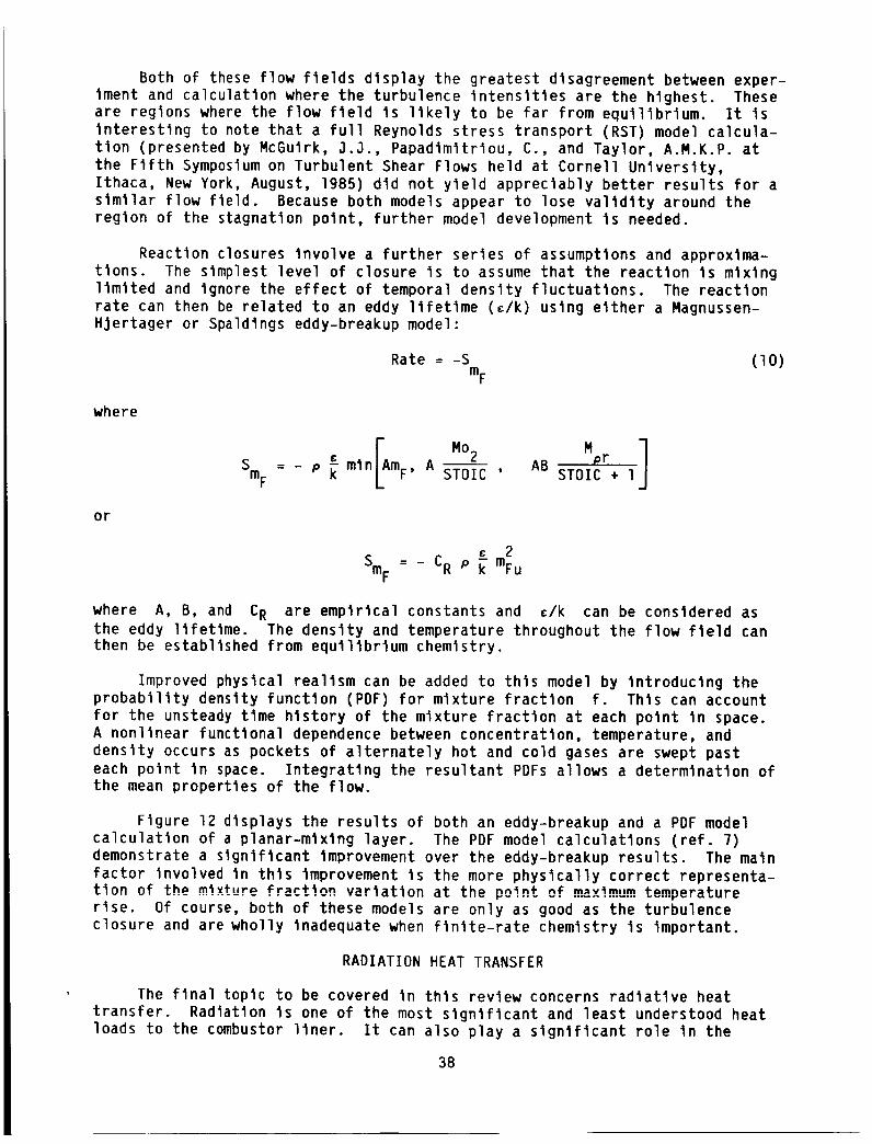
Reaction closures involve a further series of assumptions and approxima-tions. The simplest level of closure ls to assume that the reaction Is mixinglimited and lgnore the effect of temporal density fluctuations. The reactionrate can then be related to an eddy lifetime (_/k) using either a Magnussen-HJertager or Spaldlngs eddy-breakup model:
Rate = -S (I0)mF
where
= c [ASmF - p _ mln mF, A M° 2 Mpr ]STOIC ' AB STOIC + 1
or
c 2: _ CRP_m FSmF u
where A, B, and CR are empirical constants and _/k can be considered as
the eddy lifetime. The density and temperature throughout the flow field canthen be established from equilibrium chemistry.
Improved physical realism can be added to thls model by introducing the
probability density function (PDF) for mixture fraction f. Thls can account
for the unsteady tlme history of the mixture fraction at each point In space.
A nonlinear functional dependence between concentration, temperature, and
density occurs as pockets of alternately hot and cold gases are swept past
each point In space. Integrating the resultant PDFs allows a determination of
the mean properties of the flow.
Figure 12 displays the results of both an eddy-breakup and a PDF modelcalculation of a planar-mlxlng layer. The PDF model calculations (ref. 7)
demonstrate a significant improvement over the eddy-breakup results. The maln
factor involved In thls improvement Is the more physically correct representa-t!on of the mixture fraction variation at the point of maximum temperature
rise. Of course, both of these models are only as good as the turbulence
closure and are wholly inadequate when flnlte-rate chemistry is important.
RADIATION HEAT TRANSFER
The final topic to be covered in thls review concerns radiative heat
transfer. Radiation Is one of the most significant and least understood heat
loads to the combustor liner. It can also play a significant role In the
38

determination of flame temperature. Any numerical description of a gas tur-bine combustor must include a radiation heat-transfer model. The stx-fluxmodel Is the model most commonly used to approximate multidimensional radi-ative transfer. In thts model, differential equations describing the radi-ative fluxes In positive and negative directions along the principal axis aresolved:
-_x 1 dRX_ a(R x -E) , S(2R x Rr - Rz)a+Sdx/ =
Ia ) S _ Rxl d r dRr = a(Rr E) + _(2R r - Rz)r dr + S + ! dr
r
,r ÷ S r de) = a( - E) + S(2RZ - Rr)
(ll)
where
Rx,r, z composite fluxes
a absorption coefficient
S scattering coefficient
E aT 4
The maln input to this analysis concerns the optical characteristics of the
hot gas and soot which must be arbitrarily specified or calculated through asoot formation and oxidation model.
The performance of the slx-flux model (ref. 8) is displayed In figure 13.
Although the model overestimates the radiative heat transfer In comparisonwlth experimental data, the qualitative trend Is quite closely followed. Given
the large number of approximations used In the analysis, the agreement wlth
experimental data Is qulte surprising. The slx-flux model does not accuratelytreat the angular dependence of energy transfer, and the determination of the
optical characteristics of the soot cloud still remains as an area of needed
research; however, fairly good results appear to be possible In thls example.
CONCLUDING REMARKS
Perhaps the most important question any review on numerical modeling cananswer Is whether or not current computational codes can be usefully employed
In the design of combustion devices. Certainly a great deal of research is
needed before one can expect quantitative predictive accuracy, and It seems
likely that some hardware problems wlll only be resolved through development
testing. The best computer program wlll never replace the designer's innova-
tive mind, but computer predictions can be used to extend the designer's pro-
ductivity. New designs can be examined much more rapidly on the computer than
in hardware testing. Development costs can be reduced. The promise of thls
computer-based design methodology Is so great that these numerical models wlll
be used despite their deficiencies. Designers should not and probably will
39

not abandon empirical design tools, but the cautious adoption of numerical
models in the design process Is a trend which can reap important benefits.
REFERENCES
l. Leonard, B.P.: Stable and Accurate Convective Modelling Procedure Based on
Quadratic Upstream Interpolation. Comput. Methods Appl. Mech. Eng., vol.19, no. 1, June 1979, pp. 59-98.
2. Ralthby, G.D.: Skew Upstream Differencing Schemes for Problems InvolvingFluid Flow. Comput. Methods Appl. Mech. Eng., vol. 9, no. 2, Oct. 1976,pp. 153-164.
3. Boris, J.P.; and Book, D.L.: Flux Corrected Transport. I. SHASTA, A Fluid
Transport Algorithm That Works. J. Comput. Phys., vol. II, no. l,Jan. 1973, pp. 38-69.
4. Claus, R.W.; Neely, G.M.; and Syed, S.A.: Reducing Numerical Diffusion for
Incompressible Flow Calculations. NASA TM-83621, 1984.
5. Claus, R.W.: Numerical Calculation of Subsonic Jets in Crossflow WithReduced Numerical Diffusion. NASA TM-87003, 1985.
6. Launder, B.E.; and Spalding, D.B.: The Numerical Computation of Turbulent
Flows. Comput. Methods Appl. Mech. Eng, vol. 3, no. 2, Mar. 1974,pp. 269-289.
7. Farchshl, M.: Prediction of Heat Release Effects on a Mixing Layer. AIAAPaper 86-0058, Jan. 1986.
8. Srlvatsa, S.K.: Computations of Soot and NOx Emissions From Gas Turbine
Combustors. (GARRETT-REPT-21-4309, Garrett Turbine Engine Co.; NASAContract NAS3-22542.) NASA CR-167930, 1982.
TABLE I. - RATIO OF CONVERGENCE TIMES
FOR VARIOUS DIFFERENCING SCHEMES
WITH UPWIND CONVERGENCE TIMES
USED AS THE STANDARD
Mesh Upwind
Coarse (30 by 22) i
Fine (58 by 38) l
BSUDS QUICK
6.4 3.2
14.7 15.7
40

Yj+l- _ NI
r--t W I ItP i .
Yj--4 _--4-_-_---_,_--qtu" r lueL---_V S
II
Yj-l-- ,,kYS
Xi-I Xi Xi+1
I -- LOCATION VARIABLE
0 P,p,_
t v_- _ U
Figure 1. - Staggeredmeshsystem for discretizing equationsbyfinite volumemethod.
rN
n
I " I
L_.:s lIT
!ss
E EE
Figure 2. - Staggeredmesh systemforquadraticupstreaminterpolation.
NW
w_
W I
SW
r .... "-I
wL, leI
..... .J
NE1
SE;I
Figure3. - Staggeredmeshsys-tem for boundedskewupwinddifferencingscheme(BSUDS).
41

2O
lO
I.a.I
5
.6--- i _ i15 30 45
FLOW ANGLE,8, deg
Figure4.- Accuracyofvariousdifferencingschemesfor a scalartransport test calcu-lation.
i
r-_ x/H = 1
I I
3h 1 25oH ___ ....¢CC_- INLETFLOWANGLE,
Y_--.x i
/1" _ 45 h
1.0
.8
.6
.4
.2
HYBRIDQUICK
--'_%,-_,,,_ BSUDS2
- ).,j
-I0
-.4
_ /
- ,)
I_ i i i i i-.2 0 .2 .4 .6 .8 1.0 -.4 -.2 0 .2 .4 .6 .8 1.0
UIUin
la) Coarsegrid calculations, 30 by22. (b)Fine gridcalculations, 58 by 38.
Figure 5. - Laminarflowcalculationstesting various differencingschemes.
42

o
z
0
50O
4OO
3OO
2OO
10O
o4
\,
_\,,,,',,,\
I I I I I.5 .6 .? .8 .9
RELAXATION
(a) For 38 by38 gridpointcalculation.
IO00--
A SIMPLE /
0 SIMPLER /8OO
6OO
4OO
20O
lO00 2000 3000NUMBEROF GRIDPOINTS
(b) Forvarious computational meshes.
I1.0 0
I
Figure 6. - Convergencetimes.
,,-.,
>.-
-2-3
-_. L. ..............
0 3
×ID
Figure 7. -Three-dimensional jet-in-crossflowcalculation.
4
3
_2
1
0 EXPERIMENTUNIFORMBOUNDARYCONDITIONSDISTORTEDBOUNDARYCONDITIONS
ATJETORIFICE
.4 .8 1.2 1.6 2.0
AXIALVELOCITY.U/Lloo
Figure 8. - Calculatedaxial velocityprofilescom-paredwith experimentaldata.
43
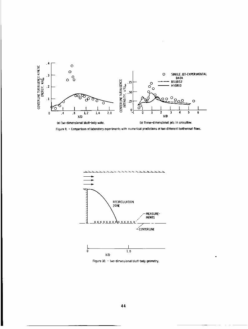
.4
.3
_JZZtJ.J
-m .I
l.aJC.)
0
0
00 0
.4 .8 1.2 1.6 2.0XTD
(a) Two-dimensionalbluff-bodywake.
0 SINGLEJET-EXPERIMENTALDATA
.15 ..... BSUDS2_ o -- HYBRID_ 0 0
_ .5o - o,.
_ .25 -- 0
g- 0 °_1 I I I I I I"i 0 1 2 3 4 5 6
XID
(b)Three-dimensionaljetsincrossflow.
Figure9. - Comparison of laboratoryexperimentswith numerical predictionsof twodifferent isothermal flows.
NERECIRCULATION
r MEASURE-/," MENTS
XXXXXXXX_X. XX XX X"7
/
_-CENTERLINE
I I0 1.0
X/D
Figure 10. - Two-dimensionalbluff-body geometry.
44

MEASURE-MENTS_.
-2-3
..... _ZAT".d¢_.-.._.. x. x .....
........ ::IIIlIZI: ................
........ ,:?ll_k/,l:.................
....... .,¢' _..................
_ .. .... liI_: _l......... :
| l I I l
0 3
XID
Figure11.-Three-dimensionaljetgeometry.
UEL I
AIR IL. -(al Example- planar mixing layer.
-. 15 _ 0 EXPERIMENT
-. lO _o_UtATION,<°-.05
>-
•10
.151o-I I I I I I I0 .2 .4 .6 .8 I.O 1.2 1.4
I
°_ ° o I
.2 .4 .6 .8NORMAUZEDTEMPERATURERISE
(b) Eddybreakupmodel. (c) PDF model.
Figure I2. - Resultsofcalculationsofa planar-mixing layer.
I1.0
45

_e
x"3la_
TEST COMBUSTOR_
/ / \BEAM PRIMARY SECONDARY TERTIARY
PATHS ZONE I ZONE 2 ZONE 3
(a)Schematic drawing ofexperimentalmeasurement
locations.
100
8O
20
0
_, CALCULATION -
T SIX-FLUX MODEL- -- - -- EXPERIMENT
_ \b
I I2 3
ZONE
(b) Performance of six-flux
model.
Figure 13. - Radiative heat transfer test calculation.
46
N87-20271
EXPERIMENTAL AND ANALYTICAL INVESTIGATION OF THE VARIATION OF SPRAY
CHARACTERISTICS ALONG A RADIAL DISTANCE DOWNSTREAM OF A
PRESSURE-SWIRL ATOMIZER
J.S. Chin, W.M. LI, and X.F. WangBelJlng Institute of Aeronautics and Astronautics
BelJlng, People's Republic of China
The variation of spray characteristics along a radial distance downstream
of a pressure-swlrl atomizer was measured by laser llght-scatterlng technology.
An analytical model was developed to predict the variation of spray character-
istics along the radial distance. A comparison of the predicted and experi-
mental data showed excellent agreement. Therefore, the spray model proposed,
although relatively simple, is correct and can be used, with some expansionand modification of the prepared model, to predict more complicated spray
systems.
INTRODUCTION
The characteristics of the spray formed by an atomizer in a llquld-fueled
combustion device are extremely important to the performance, stability, and
pollutant formation of the combustor. The spray characteristics should be
measured accurately, and a model should be developed to predict the variation
of spray characteristics, droplet trajectory, spray dispersion, and evapora-
tion history. It is also important to understand the influence of variousfactors on the measurement of spray characteristics. A comparison between
predicted and measured spray characteristics provides useful insight intospray combustion. Such research has a slgnlflcant effect on engineering
applications and on the fundamental understanding of spray combustion.
The authors analyzed the variation of spray characteristics along the
axial distance downstream of a pressure-swirl atomizer. The effect of spray
evaporation on the variation of spray characteristics is discussed inreference 1 and was presented by J.S. Chin and J.Y. Zhu at this symposium.
(Paper, entitled The Interdependence of Spray Characteristics and Evaporation
History of Fuel Sprays in High Temperature Airflows, was unavailable for
printing at the time of publication.) The influence of downstream distance onthe spray characteristics of pressure-swirl atomizers is caused by the effects
of spray dispersion and drop acceleration or deceleration. This condltlon is
analyzed in reference 2. These analyses have been partially substantiated by
some experimental data. Until now there have been few experimental data of
the variation of spray characteristics along the radial distance downstream of
the pressure-swlrl atomizer. Lee Dodge published his measurement results asshown in figure 1 (ref. 3). He shows that both the Sauter mean diameter SMD
and drop-slze distribution parameter N increase with radial distance. There
is no analysis on this aspect available at the present time.
We are interested in comparing the experimental and predicted values of
the variation of spray characterlstlcs along the radial distance. Therefore,we carefully measured this variation in a well-deflned experimental condition,
"developed an analytical model to predict the variation, and then compared the
47
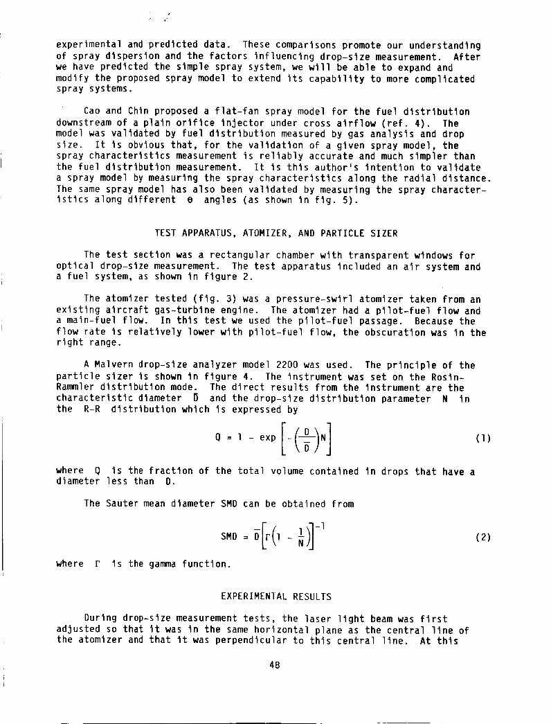
experimental and predicted data. These comparisons promote our understanding
of spray dispersion and the factors influencing drop-slze measurement. After
we have predicted the simple spray system, we will be able to expand and
modify the proposed spray model to extend its capability to more complicatedspray systems.
Cao and Chin proposed a flat-fan spray model for the fuel distribution
downstream of a plain orifice injector under cross airflow (ref. 4). Themodel was validated by fuel distribution measured by gas analysis and drop
size. It is obvious that, for the validation of a given spray model, thespray characteristics measurement is reliably accurate and much simpler thanthe fuel distribution measurement. It is this author's intention to validate
a spray model by measuring the spray characteristics along the radial distance.
The same spray model has also been validated by measuring the spray character-istics along different B angles (as shown in fig. 5).
TEST APPARATUS, ATOMIZER, AND PARTICLE SIZER
The test section was a rectangular chamber with transparent windows for
optical drop-slze measurement. The test apparatus included an air system anda fuel system, as shown in figure 2.
The atomizer tested (fig. 3) was a pressure-swlrl atomizer taken from an
existing aircraft gas-turblne engine. The atomizer had a pilot-fuel flow anda main-fuel flow. In this test we used the pilot-fuel passage. Because the
flow rate is relatively lower with pilot-fuel flow, the obscuratlon was In theright range.
A Malvern drop-slze analyzer model 2200 was used. The principle of the
particle slzer is shown in figure 4. The instrument was set on the Rosin-Rammler distribution mode. The direct results from the instrument are the
characteristic diameter B and the drop-slze distribution parameter N in
the R-R distribution which is expressed by
exo[,N] (I)
where Q is the fractlon of the total volume contained in drops that have adiameter less than D.
The Sauter mean diameter SMD can be obtained from
where r is the gamma function.
(2)
EXPERIMENTAL RESULTS
During drop-size measurement tests, the laser light beam was first
adjusted so that it was in the same horizontal plane as the central line ofthe atomizer and that it was perpendicular to this central llne. At this
48

position (defined as the y = 0 position), the spray characteristics weremeasured. Then the Malvern particle slzer was put on some stze blocks ofknown dimension. This changed the height of the laser beam so that the radtaldistance where the parttcle stzer measured the drop stze was changed. Thesummation of the size block was defined as the radlal distance y. The dlmen-slons of the blocks chosen were 2.5, 3.0, and l0 mm. Thus, the followingradial distance y could be obtained by different combinations of the sizeblocks: y = 0, 5.5, 10.0, 15.5, 20.0, 25.5, and 30.0 mm. The experimentalresults are shown In figures 6 to 13. From these figures it Is clear that theSauter mean diameter and drop-size distribution parameter increase with radialdistance until the edge of the spray has been reached. The experlmentalresults obtained by the present authors are quantitatively tn good agreementwith Lee Dodge's results. The obvious explanation of the measured resultsshown in figures 6 to 13 is that wtth larger radial distances the possibilityof the laser light beam meeting the large drops ts greater than tt is withsmaller radtal distances. Thts shows that when we measure the drop size it tsnecessary to take a sample that Is representative of the spray formed; how-ever, it ls impossible to define the sample which would fully represent thespray. The most reasonable sample can be obtained by measuring the spray atthe y = 0 position.
Comparing figure 6 wlth 8 and 7 wlth 9 shows that, at a higher airflow
velocity, the change of spray characteristics along the radial distance Is
weaker. A comparison of figures 8, lO, and 12 and of 9, II, and 13 shows
that, wlth a lower pressure drop across the nozzle, the change of the spray
characteristics along the radial distance Is weaker. These results tell us
that when the spray Is expanded less radially the change of spray characteris-tics is also flatter. The reverse Is also true.
The experimental data obtained In thls way were used to check the pro-
posed spray model.
PHYSICAL MODEL
The spray formed by a pressure-swlrl atomizer Is shown In figure 5. The
physical model was proposed wlth the following assumptions:
(I) The atomization process is completed as soon as the fuel leaves the
atomizer nozzle; that Is, droplets of different sizes start their movement at
the nozzle exit. Droplets of different sizes have the same initial velocity.Because It Is suitable to use a cylindrical coordinate system to describe
droplet motion, the tangential velocity and the radial velocity component canbe combined and treated as one velocity component.
(2) The airflow Is uniform.
(3) The air Is at ambient temperature, so droplet evaporation can beneglected.
(4) The influence of different droplet velocities on the drop-slze meas-
urements made by the Malvern particle slzer Is neglected.
The initial drop-slze distribution can be expressed by Do(SMDo) and No
wlth the initial volume fraction (dQ/dD) o as
49

N -l
No l°dD o DO(3)
At a downstream distance x, the droplets of diameter D move from the origin
and then distribute themselves on a circumference of radius R(D) while the
laser light beam of diameter dj only meets some of these droplets:
(4)
where
1
Yo - 2 dj
mI = arcsln R(D) (5)
1
Yo + 2 dj
m2 = arcsln R(D) (6)
The definitions of m2 and _I are shown in figure 5. When
Yo - 1 dj <_ R(D) <_ Yo + 1 dj
then
_o2 =
where Yo is the radial distance and dj the diameter of the light beam.
The summation of the liquid fraction of the droplets of various diameters
passing through the laser light beam is given by
dD (7)
The minimum diameter Dml n that the laser light beam can see is determinedby
R(Dmln) = Yo - ½ dj
That is, at the downstream distance x, if
will not pass through the laser light beam.
determined by the droplet motion equation.
exist in the spray, can be approximated by
R(D) < Yo - 1/2 dj, this dropletThe relationship R(D) can be
The maximum diameter that may
50
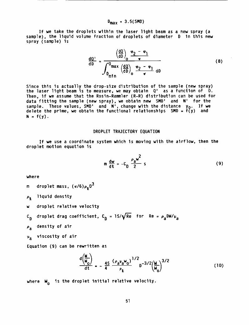
Omax = 3.5(SMD)
If we take the droplets within the laser light beam as a new spray (a
sample), the liquid volume fraction of droplets of diameter D in this newspray (sample) is
dQ _2 - _ldQ'_ dD odD
-f Dmax (dd-d-_D/o_2- _lJ Dml n
dD
Since this Is actually the drop-slze dlstrlbution of the sample (new spray)the laser light beam is to measure, we may obtain Q' as a function of D.
Then, if we assume that the Rosln-Rammler (R-R) distribution can be used for
data fitting the sample (new spray), we obtain new SMD' and N' for the
sample. These values, SMD' and N', change with the distance Yo- If wedelete the prime, we obtain the functional relationships SMD = f(y) and
N = f(y).
(8)
DROPLET TRA3ECTORY EQUATION
If we use a coordinate system which is moving with the airflow, then the
droplet motion equation is
where
m droplet mass, (_/6)ptO3
p_ liquid density
w droplet relative velocity
CD droplet drag coefficient, CD
Pa density of air
_a viscosity of air
Equation (9) can be rewritten as
dt - -
where Wo
2dw Paw
m _ = -CO 2
= 15/_/'_ for Re = PaDW/Pa
45 (PaPaWo )l/2D_3/2(W _3/2
4 Pl. \Wo)
is the droplet initial relative velocity.
(9)
(lO)
51
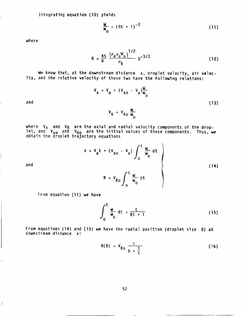
Integrating equation (lO) yields
W )-2_--= (Bt + 1 (II)0
where
45 (Pa"aWo )I/2= -- D-3/2
B 8 p_ (12)
We know that, at the downstream distance x, droplet velocity, air veloc-
ity, and the relative velocity of these two have the following relations:
+( wVx = Va Vxo - Va)_--
0
and (13)
WVR = VRo _--
0
where Vx and VR are the axial and radial velocity components of the drop-
let, and Vxo and VRo are the initial values of these components. Thus, weobtain the droplet trajectory equations
and
_o t Wx = Vat + (Vxo - Va) Woo dt
_o t WR = VRo Woo dt
(14)
From equation (ll) we have
t
_o W dt tWoo -Bt+l(15)
From equations (14) and (15) we have the radial position (droplet size D) atdownstream distance x:
lR(D) = VRo ] (16)
B+_
52
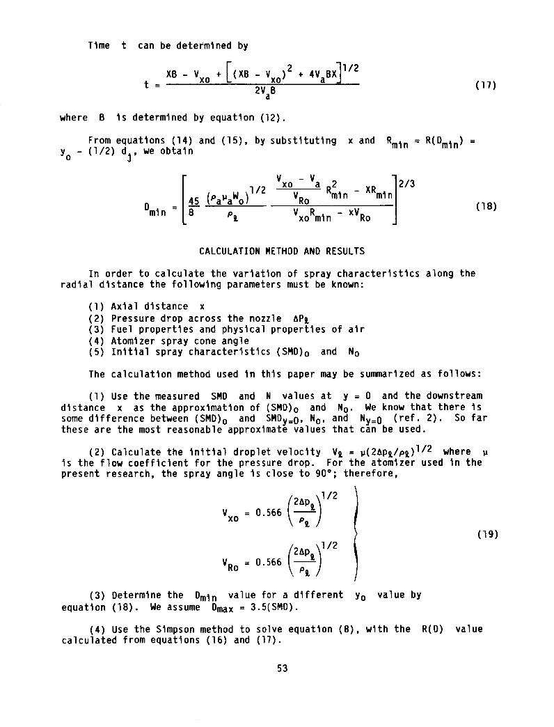
Time t can be determined by
r)2 4VaBX]I/2XB - Vxo + L(XB - Vxo ÷
t =2VaB
(17)
where B Is determined by equation (12).
From equations (14) and (15), by substituting x and Rml n = R(Dml n) =
Yo - (1/2) d_, we obtain
I v 1Vxo - a _2 2/3
Dmln = 84_55(Pa"aWo)I/2 VR0- Kml n - XRmlVxo m n- " (18)
CALCULATION METHOD AND RESULTS
In order to calculate the variation of spray characteristics along theradial distance the following parameters must be known:
(1) Axial distance x
(2) Pressure drop across the nozzle aP_
(3) Fuel properties and physical properties of alr
(4) Atomizer spray cone angle
(5) Initial spray characteristics (SMD)o and No
The calculation method used In thls paper may be summarized as follows:
(1) Use the measured SMD and N values at y = 0 and the downstream
distance x as the approximation of (SMD) o and NO. We know that there Is
some difference between (SMD) o and SMDy= O, NO, and Ny= 0 (ref. 2). So farthese are the most reasonable approximate values that can be used.
(2) Calculate the initial droplet velocity Vt = _(2ap_Ipt) I/2 where
Is the flow coefficient for the pressure drop. For the atomizer used In the
present research, the spray angle Is close to 90°; therefore,
Vxo = 0.566
2Aptll/2VRo = 0.566
(19)
(3) Determine the Omln value for a different Yo value by
equation (18). We assume Dmax = 3.5(SMD).
(4) Use the Simpson method to solve equation (8), wlth the R(D) value
calculated from equations (16) and (17).
53

(5) Determine the integration
Q' = dD
mln
From this, we are able to obtain a set of the data of Q' and D.
(6) Assume that Q' can be fitted by R-R distribution:
Q' = 1 - exp -
By using the least-square method, we can obtain D and N'; then, SMD' and
N' can be calculated. These SMD' and N' values are plotted against y
in figures 6 to 13.
The results of the calculations for different airflow velocities and for
the nozzle pressure drop are shown in figures 6 to 13. These are compared
with the corresponding experimental data. It is obvious that the predictions
are in excellent agreement with the experimental results.
CONCLUDING REMARKS
In the present study, droplet evaporation was neglected (discussed by
J.S. Chin and J.Y. Zhu in the unpublished paper cited previously), and it is
not difficult to take into consideration the effect of droplet evaporation.
After this model has been validated, it is relatively simple to predictthe fuel distribution downstream of a pressure-swirl atomizer (ref. 6).
One interesting point that was noticed from the experiments and the anal-
ysis was that the larger droplets are always at the spray edge. Because the
ignition spark plug is also always positioned close to the spray edge, the
spark might meet the larger droplets, which would harm the ignition.
We measured the variation of spray characteristics along the radial dis-tance was by laser light-scatterlng technology. And we found that the predic-
tion based on the proposed spray model was in excellent agreement with theexperimental data.
l °
.
REFERENCES
J.S. Chin; R. Durrent; and A.H. Lefebvre: The Interdependence of Sprayrh_+o_+_ _,a _,,_^_+_ _+.... ^_ _,,ol _,,_ Transacti_ _....................... _, _,on Hi_, j ....... v,_ ........
ASME Journal of Engineering for Gas Turbine and Power. July, lgB4.
J.S. Chin; D. Nickolaus; and A.H. Lefebvre: Influence of Downstream
Distance on the Spray Characteristics of Pressure-Swirl Atomizers. ASME
85-GT-138, Transactions of the ASME, Journal of Engineering for GasTurbine and Power, Jan., 1986.
54

.
.
.
.
L.G. Dodge; and C.A. Moses: Mechanisms of Smoke Reduction In the HtghPressure Combustion of Emulsified Fuels. Vol. 1, Construction of Appara-tus and Preliminary Experiments, Yearly Progress Report No. l, Sept. 29,1980 to Sept. 29, 1981.
M.H. Cao; J.S. Chin; et al.: Semi-Empirical Analysis of Liquid FuelDistribution Downstream of a Plain Orifice Injector Under Cross-streamAir Flow. Transactions of the ASME, Journal of Engineering for Power,Oct., 1982.
3.S. Chtn; X.F. Wang; W.M. Lt; and A.H. Lefebvre: The Influence onMeasured Spray Characteristics of Variations In the Radtal and AngularPositions of the Sampling Laser Beam. Spring Technical Meeting CentralStates Sectlon/The Combustion Institute, Paper CSS/CI 86-5C1, 1986.
3.S. Chin; and A.H. Lefebvre: Predlctlon of Ltquid Fuel DlstrlbutionDownstream of a Swirl Atomtzer In Flowing Air. Sprlng Technical Meettng,Central States Section/The Combustion Institute, Paper CSS/CI 83-20, 1983.
55

E _
Et_
t-f_aJE
i-
V3
gO
8£,
70
6o
40
IOO
9o
80
qo
6o
50
J
; S /
J
i , I , I I _ I I J I ,
0 2 _ 6 8 10 1_ 1@ 16
(a) x = 25.4 mm.
-",0
_8
(b) x = 50.8 ram.
,2.4,
2.2,
_0
i;:1.._,
._6
_2
_,o
2.6
2.4,
2.0
16
30
z
C_u
E11:1
co
N
I
0L
Figure 1. - Lee Dodge's measurement resu]ts (ref. 4). Atomlzer
pressure drop, _P, ]00 ]b/In. 2
56

2
4 5
f
12
lOf .._-
14/5__ )
Figure 2. - Experimental system. Plenum chamber, 1; airtemperature, 2; air flowmeter, 3; test section, 4; exhaustpipe, 5; fuel tank, 6; fl]ter, 7; pump, 8; return valve, 9;valve, 10; pilot-fuel flow valve, 11; pressure gauge, 12;atomizer, 13; main-fuel flow valve, 14; pressure gauge, 15.
2
Figure 3. - Atomizer. Pllot-fuel
flow, I; maln-fuel flow, 2.
57

12
Figure 4. - Laser drop particle slzer. Laser, l; beam expander, 2; testsection, 3; fuel nozzle, 4; lens, 5; photo detector, 6; solid valve, 7;
amplifier, 8; A/D converter, 9; data transfer, lO; interface, ll;
computer, 12; printer, 13; micro tune, 14.
--" Spray--_. i Lightt Y .J_ Beam
---_ / f ,T-'Cq)-- o_- _O%v,
-Xv- iz Fuel
Laser LightBeam
Figure 5. - Physical model.
58
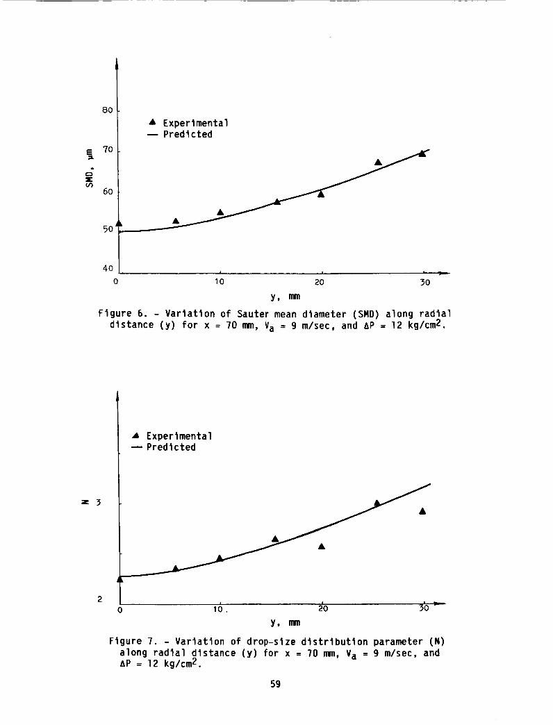
E
:E
80
70
60
50
• ExperimentalPredicted
40 , ,o lO 20 30
y, mm
Ftgure 6. - Variation of Sauter mean diameter (SMD) along radtaldistance (y) for x = 70 mm, Va = 9 m/sec, and AP = 12 kg/cm2.
z 3
• Experimentaln Predtcted
o 3by, Inm
Figure 7. - Varlatlon of drop-size distribution parameter (N)
along radial dlstance (y) for x = 70 mm, Va = 9 m/sec, and&P = 12 kg/cm 2.
59

E
u_
8O
70
6O
5O
40
• ExperimentalPredicted
i i
0 I0 20 30
y, mm
Figure 8. - Variation of Sauter mean diameter (SMO) along radial
distance (y) for x = 70 mm, Va = 6 m/sec, and AP = 12 kg/cm2.
z 3
0
ExperimentalPredicted
10 20 30
y, mm
Figure 9. - Variation of drop-slze distribution parameter (N) along
radial distance (y) for x = 70 mm, Va = 6 m/sec, andAP = 12 kg/cm2.
60
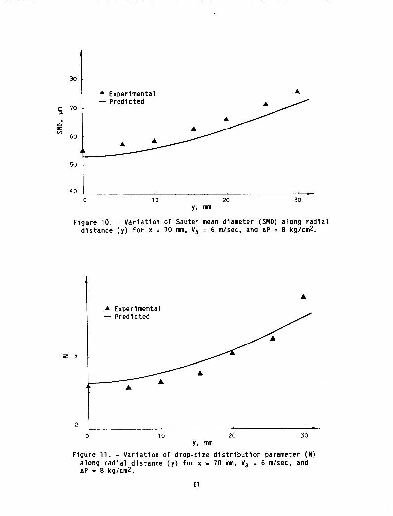
80
E 7o
s'-
6O
50
40
• Experimental A
-- Predicted ,&_
0 I 0 20 30
y, mm
Figure I0. - Variation of Sauter mean diameter (SMD) along radial
distance (y) for x = 70 mm, Va = 6 m/sec, and AP = 8 kg/cm2.
z 3
___ Experlmental
k
L t i
0 I0 20 30
y, mm
Figure II. - Variation of drop-slze distribution parameter (N)
along radial distance (y) for x = 70 mm, Va = 6 m/sec, and
AP = 8 kg/cm2.
61

E;z
C:3
zu3
7O
6O
50
• Experimental-- Predlcted
4O
0 10 20 30
Figure 12. - Variation of Sauter mean diameter (SRD) along radialdistance (y) for x = 70 mm, Va = 6 m/sec, and AP = 4 kg/cm L.
z 3
• Experimental-- Predicted
I I |
0 I0 20 30
Figure 13. - Variation of drop-size distribution parameter (N)along radial dlstance (y) for x = 70 mm, Va = 6 m/sec, and_P = 4 kglcm 2.
62

TWO-PHASE FLOW
Robert R. Taclna
NASA Lewis Research Center
Cleveland, Ohio
87-20272
An experimental program to characterize the spray from candidate nozzlesfor Iclng-cloud simulation is discussed. One candidate nozzle, which is cur-
rently used for icing research, has been characterized for flow and drop size.
The medlan-volume diameter (MVD) from this alr-asslst nozzle is compared with
correlations in the literature. The new experimental spray facility is dis-
cussed, and the drop-slze instruments are discussed in detail. Since there is
no absolute standard for drop-slze measurements and there are other limita-
tions, such as drop-slze range and velocity range, several instruments are used
and the results are compared. The drop-slze instruments used are the Malvern
2600, the NASA Lewis Scanning Radiometer, the Phase/Doppler Spray Analyzer
(P/DSA), a Forward-Scatterlng Spectrometer Probe (FSSP), an Optical Array Probe
(OAP), and a limited amount of photography. The known capabilities and llml-
tations of the drop-slze instruments are compared.
A two-phase model was developed at Pennsylvania State University. Themodel uses the k-c model of turbulence in the contlnous phase. Three methods
for treating the discrete phase are used: (1) a locally homogenous flow (LHF)
model, (2) a deterministic separated flow (DSF) model, and (3) a stochastic
separated flow (SSF) model. In the LHF model both phases have the same veloc-
ity and temperature at each point. The DSF model provides Interphase transport
but ignores the effects of turbulent fluctuations. In the SSF model the dropsinteract with turbulent eddies whose properties are determined by the k-c
turbulence model. The two-phase flow model has been extended to include the
effects of evaporation and combustion. Model development has been accompanied
by an experimental program to provide data for verification. Presently, themodel has been further extended at NASA Lewis to include the effects of
swirling flow, and a partlcle-laden swirling flow experiment is currentlybeing performed to provide verification data.
INTRODUCTION
Sprays and two-phase flow are of interest in many fields - for example,
gas turbine combustion, agricultural crop spraying, paint spraying, fire pro-
tection, and drying. This paper describes the use of sprays to simulate icing
clouds for the Altitude Wind Tunnel Icing Research Program. Iclng-cloud simu-
lation and gas turbine combustion research have common interests in the method
of injection, the characterization of drop size and of droplet velocities, and
the development of analytical models for droplet trajectories and droplet
vaporization. This paper discusses injector or spray-nozzle drop-slze charac-
terization, an experimental test facility for injector characterization, drop-
size measurement techniques, and analytical models for trajectory calculations.
IN3ECTOR CHARACTERIZATION
The injector, or spray nozzle, used currently for Iclng-cloud simulationat the NASA Lewis Research Center is an alr-asslst injector (fig. l). It is
63
very similar to the injector used by Nuklyama and Tanasawa (ref. 1). The water
flows through a center tube (0.635-mm dlam) and has a concentric annular pas-
sage (9.35-mm dlam) for alr-asslst flow. The water and the air exit through a
3.175-mm orifice. The advantage of an alr-asslst injector for icing research
and other applications is that, within limits, there Is nearly independent
control of water flowrate and drop size. The water flow Is controlled by the
difference between the air pressure and water pressure, and the drop slze Is
controlled by the alr pressure only.
Drop-slze measurements using this injector were made for us at ArnoldEngineering Development Center by J.L. Hunt. The drop-slze data shown In
figure 2 are plotted as medlan-volume diameter in micrometers. The median-
volume diameter MVD is defined as the drop size where 50 percent of the total
droplet volume is contained in droplets less than that diameter, and 50 percent
is contained In droplets greater than that diameter. The MVD is plotted as a
function of the difference of water and alr-asslst pressure wlth the air-
assist pressure as a parameter.
This method of correlating the data is very useful for setting the oper-
ating conditions in the wind tunnel. However, the drop-slze data could be
presented in a more fundamental manner as a function of the water to air mass
ratio. Other factors that appear in correlations In the literature, such as
viscosity, surface tension, and relative velocity between the air and water,
are constant or nearly constant for these data. The relative velocity Is
nearly constant, even though the flowrates are changing. The reason for this
Is, first, that the alr Is being injected at high pressure into a low-pressure
ambient environment and thus has sonic, or nearly sonic, velocity. Second, the
water pressure is relatively low so that the water has a relatively small
velocity compared to the sonic velocity of the air. Thus, the difference In
the velocities or the relative velocity is constant.
These data were compared to values from various correlations. These com-
parisons are shown in figure 3 for one alr-asslst pressure. The injectors used
in the references were similar to the NASA Lewis Research Center injector.
However, the drop-slze measurement techniques were different. The Nuklyama-
Tanasawa (ref. l) drop-slze correlation was made from measurements of water
droplets on photographs. The Lorenzetto-Lefebvre correlation (ref. 2) was made
from llght-scatterlng measurements of water droplets. Wlgg (ref. 3) used
measurements from molten wax sprays with swirl. As you can see in the figure,
the results of the correlations have a wide range of values, some higher and
some lower than the data taken at Arnold. Preliminary data taken at NASA
Lewis seem to be closest to the data of Nuklyama-Tanasawa. Preliminary
data taken With the NASA Lewis injector at Carnegle-Mellon University are lower
than the Arnold data. There needs to be much more work on drop-slze measure-
ments and correlations before drop sizes can be accurately predicted.
TEST FACILITY
The objectives of our experimental program are to characterize a varietyof candidate injectors for drop size and dispersion, to compare different
drop-size measurement techniques, and to take data that can be used for tra-
jectory models. Trajectory model data consist of initial condition data taken
upstream close to the injector and verification data taken far downstream.
64

The test stand is shown In figure 4. Duct air enters through a 40-cm-diameter pipe. The maximum atr velocity through the pipe is 88 m/sec. We wtllbe able to control the relative humldtty from 0 to 100 percent by adding steam
far upstream. Controlling the relative humidity could be necessary tf evap-oration ts important.
The duct atr temperature wtll be controlled by injecting ltquid nitrogenupstream. The primary use of the temperature control will be to provide aconstant Inlet temperature of 292 K. For some icing tests the Inlet temper-ature Is held at 273 K and even lower temperatures for shorter times.
The injector ts inserted In a section with a window so that the nozzleoperation can be monitored wtth a television camera. Water ts the only liquidcapable of being tested in this facility. The water is demlnerallzed andheated to 380 K. For icing applications, the water and the air-assist injectorare heated so that tce crystals do not form during the expansion process. Thewater and air-assist flow temperature can be controlled between the ambienttemperature and 3?3 K.
The injector ts shown In a section 2.5 m upstream of the instrument sec-tion. The injection section can be moved to any location closer to theinstrument section. Upstream of the injector there ts a traversing pltot tubeto measure the Inlet velocity.
Downstream, at the instrument section, drop-size measurements can be made.The instrument section has a square cross section wtth windows In the sidesthat are at 7° angles to each other to prevent reflections. Other drop-sizeinstruments that are used are described In the next section. The instrumentsstt on a three-axis traversing table so that radial and spatial variations canbe measured. A llquld-water measurement probe traverses vertically to measurethe variation in liquid-water concentration.
Another set of droplet-sizing instruments Is mounted In the duct down-stream of the instrument section. The principle of operation of these instru-ments ts discussed In the next section. These instruments are intrusive andmounted In a fixed position. They are the same instruments that are mountedon airplanes to measure drop sizes In clouds. Tests with these instrumentswill provide a good comparison of the data from the nozzles with that In theclouds. This Is an atmospheric pressure rtg, so the atr and water are ventedto the atmosphere.
DROP-SIZE INSTRUMENTS
The most important factor In making drop-slze measurements is the drop-
slze measuring instrument. As you have seen from the figure comparing the
drop-slze data correlations, there must be large differences in the data on
which they are based. One of the major problems is that there Is no standardto which to compare the drop-slze measurements, especially In a spray. Since
there are other limitations beside the lack of a standard such as drop-slze
range and velocity range, In our program we use five different drop-slzeinstruments and compare the results. The instruments are a Malvern 2600, a
NASA Lewis Scattered-Llght Scanner, a Phase/Doppler Spray Analyzer, a Forward-
Scattering Spectrometer Probe, and an Optical Array Probe. And a limited
65

amount of photography is used for qualitative analysis. A qualitative analysisand a discussion of each of these instruments follows.
The Malvern 2600 is a commonly used drop-slze instrument (fig. 5). Lewis'HSD version of this instrument, which provides a faster snapshot of the data,
is described in reference 4. (The inserts in figure 5 describe the principle
of operation.) This instrument measures the angle that the light is diffracted
by the drops. The bigger drops diffract the light at a small angle and thesmaller drops diffract the light at a larger angle. The detector is a series
of concentric rings that determine the angle of the scattered light. The dropsize is calculated from the scattered light angle. The insert also shows that,
no matter where the droplet is in the llne of sight, the light that is scat-tered at the same angle always falls on the same detector ring.
Although there is no standard for determining drop sizes, we use a
Hirleman reticle for calibration purposes. The Hirleman reticle (fig. 6) con-
sists of a glass substrate on which chrome disks are photographically depos-ited. The chrome disks are sized to represent a Rosln-Rammler distribution
with an x-bar of 50 and an n value of 3. One problem we have found usingthe reticle with the Malvern 2600 is that there is a correction for anomalous
diffraction. The Malvern calculations are based primarily on Fraunfaufer dif-
fraction theory. However, for small drop sizes (below a diameter of 5 pm)
three-dimensional effects are considered; these effects are lumped under the
term anomalous diffraction. Thus, the problem is that the reticle has two-
dimensional disks and not three-dimenslonal spheres. We are currently studying
the feaslblllty of modifying the Malvern software to ignore the anomalous dif-
fraction calculation when using the reticle. If this does not prove to bepractical, we will still use the reticle for relative comparisons.
We also plan to add an additional lens system to the Malvern to be ableto measure an MVD of 5 pm across the 30-cm instrument section. Verification
of the correctness of the additional lens system will be done by taking meas-
urements of the retlcle with and without the additional lens system.
The second instrument, the Scattered-Light Scanner, is also based on the
diffraction principle. This is a revised version of the NASA Lewis Scanning
Radiometer (described in ref. 5), which was developed by Don Buchele and used
in many research projects by Robert Ingebo. Figures 7 to 9 explain the oper-ation of the instrument.
Figure 7 shows the reflection, refraction, and dlffractlon of a laser
light beam passing through a drop. Since calculations are based on the dif-
fraction of light through the drop, the wlde-angle diffraction is ignored.
There is narrow-angle diffracted light from the envelope (or aperture) of the
laser beam that must also be ignored.
F!gur_ R(a) It a plot of light intensity as a function of the llght-scat-
ter angle. Figure 8(b) shows the product of the light intensity and the llght-
scatter angle as a function of the light-scatter angle. It shows that the
measurement interval extends from where the intensity of the near envelope
diffraction is negligible to a value of the light intensity which is still highenough to be meaningful. A scanner is used to measure the intensity of the
scattered light as a function of the light scatter angle. The scanner is a
66

disk wtth a radial slot that is rotated wtth Its centerltne eccentric to thelaser beam centerltne.
To calculate the mean drop size, Don Buchele has calculated the lightintensity as a function of a beam spread parameter (fig. 9). From the previousfigure we can find the maximum ltght intensity and the light intensity at aspecified angle. Using these values and the beam spread parameter and knowingthe wave length and the specified angle, we can determine the mean drop size.Calculations were made wtth five different distribution correlations, and theyare shown plotted for three dispersion levels. The distribution correlationsused were the Nuktyama-Tanasawa, the upper-limit distribution functions, theRostn-Rammler, the Nelbel, and the Rinks distribution function. The beam-spread parameter ts nearly the same for all the distributions and dispersionsat a relative intensity of 0.75. If this relative intensity Is used, then themean drop-size calculation ts independent of distribution and dispersion. Thedispersion can be calculated from the slope of the curve.
A schematic of the Scattered Light Scanner (fig. 10) shows the variousparts and dimensions of the instrument. The primary feature ts the eccentriclight scanner.
The third drop-slze instrument to be discussed was developed under a NASAcombustion fundamentals contract to Wtlltam Bachello at Aerometrlcs Corpora-tion. The method Is the phase/Doppler detection technique and the instrumentts called the Phase/Doppler Spray Analyzer (ref. 6). This ts a scheme where aset of laser beams Is crossed to form a fringe pattern (fig. 11). As a drop-let passes through the fringes the llght ts scattered and measured 30 ° off axiswith a photodetector. From this measurement, simultaneous values of dropdiameter and velocity can be calculated. The measurement and calculations arefor single droplets; averages and medians are calculated from the single drop-let data.
Figure 12 shows In more detail the principle of the phase/Doppler system.The scattered light ts collected by three detectors wtth sllghtly differentspattal locations. Because of the spatial difference, the light path to thethree detectors ts different, and thus there Is a phase difference In the stg-nals. From this phase dlfference the drop stze can be calculated. Again, thephase difference occurs because of the path difference inside the drop, so thatthe phase angle Is a function of the diameter.
Figure 12(b) ts a plot of phase difference as a function of diameter.From the phase difference between detectors 1 and 2, an approximate drop-sizeestimate can be made. From this approximate drop stze and the phase differencebetween detectors 1 and 3, a more accurate determination of diameter can bemade.
The calculations are based on reflection and refraction theory. Dlffrac-tlon can be ignored because the measurements are taken 30 ° off axis, wherediffraction ts negligible.
The Forward-Scattering Spectrometer Probe (FSSP) Is one of the two lntru-stve instruments that we use that ts located downstream of the instrument sec-tion. This instrument Is the same type that Is mounted on airplanes to measureraindrop diameters (see ref. 7). It provides a comparison of the other drop-stze instrument measurements wtth the measurements made tn clouds.
67

The FSSP Is a single particle counter. A schematic of tts operation tsshown In figure 13. A laser beam. ts optically directed across two arms of theprobe, In a direction perpendicular to that of the partlcle-laden flow. Scat-tered light from a particle Is optically directed and focused onto a photodtodeto measure the intensity of the scattered light. Any unscattered light Isremoved by the dump spot. The scattered light is also directed onto a secondphotodetector that Is used to determine whether the droplet ts In focus (infocus along the axial length of the laser beam). This second photodetectoralso has a dump spot. The light from a droplet that is In focus Is removed bythe dump spot. A droplet that Is not in focus has a broader signal that ts notremoved by the dump spot, and the droplet measurement Is rejected.
Drop slze as a function of the measured intensity Is shown In figure 14.In the figure the light intensity Is shown In the near forward-scatterlng
angles of 4° to 14°. The curve Is shown for a Gausslan T-type (transverse
electric) beam. This Is a multlvalued function; thus, for a given intensity,
the drop slze may not be uniquely determined. The actual instrument uses a
hlgh-mode laser beam which has a smooth curve and Is single valued.
The last drop-slze instrument to be discussed Is the Optical Array Probe
(OAP), which can also be flown on an airplane to measure raindrop sizes. Thls
instrument Is made by the same company as the FSSP, but It Is made to cover alarger drop-slze range. The operating principle Is shown In figure 15. It Is
a slngle-partlcle imaging system. The drops pass through a laser beam, and
then the light is transmitted through the instrument optics to an array of
photodetectors. The drop slze Is determined by counting the detectors In the
shadow of the drop. The last detector at each end is kept open as a check to
determine If the whole drop Is seen. To determine If the drop Is In focus, we
use an intensity gradient criteria. An Infocus drop has a sharp gradient from
llt to unlit photodetectors, while an out-of-focus drop has a gradual gradient
from llt to unlit. Figure 16 Is a simple schematic of the OAP.
Table I compares the FSSP, OAP, Malvern 2600, Scattered-Llght Scanner, and
Phase/Doppler Particle Analyzer (P/DSA) drop-slze instruments. The slze range
refers to the droplet diameters that can be measured wlth any particular setup.
The number of bins refers to the number of increments Into which the size range
is divided. The overall slze range then refers to the smallest to the largest
diameter that can be measured, but It may require a change In setup and multi-
ple measurements to cover the range. The numbers In the ranges refer to indi-
vidual droplets for all the instruments except for the Scattered Light Scanner,
whose range Is given In MVD.
The velocity limits are all acceptable for our work except for those of
the P/DSA, which has a slight limitation for our purposes. Currently manufac-
tured P/DSA instruments have a upper limit of 75 m/sec. The comments section
lists features that we consider particularly beneficial. With the FSSP and
OAP, we consl _-- the ability to use the same I.......... to A_-In _UQ LQu_w fromU_ L_Ulll_ll LI1_ LI
clouds and the test factllty to be important. The Malvern and the Scattered-Light Scanner have the abtltty to measure MVD directly and thus are good forscreening a number of injectors qulckly. The P/DSA has the capability ofmaking point measurements of stze and veloclty which makes the data particu-larly useful for modeling work.
68
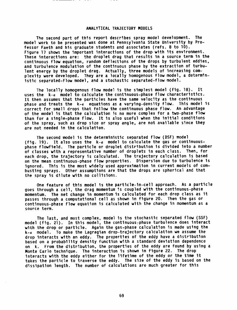
ANALYTICAL TRAJECTORY MODELS
The second part of thts report describes spray model development. Themodel work to be presented was done at Pennsylvania State University by Pro-fessor Faeth and his graduate students and associates (refs. 8 to 10).Ftgure 17 shows the Important Interactions of the drop with Its environment.These Interactions are: the drop]et drag that results tn a source term tn thecontinuous flow equation, random deflections of the drops by turbulent eddtes,and turbulence modulation of the continuous phase by the extraction of turbu-lent energy by the droplet drag. Actually, three models of Increasing com-plextty were developed. They are a locally homogenous flow model, a determln-tstlc separated-flow model, and a stochastic separated-flow model.
The locally homogenous flow model ts the simplest model (ftg. 18). Ituses the k-c model to calculate the continuous-phase flow characteristics.It then assumes that the particles have the same velocity as the continuousphase and treats the k-c equations as a varying-density flow. This model Iscorrect for small drops that follow the continuous phase flow. An advantageof the model ts that the calculation Is no more complex for a two-phase flowthan for a single-phase flow. It Is also useful when the lntttal conditionsof the spray, such as drop size or spray angle, are not available since theyare not needed tn the calculation.
The second model Is the deterministic separated flow (DSF) model(fig. 19). It also uses the k-c model to calculate the gas or continuous-phase flowfleld. The parttcle or droplet distribution Is dtvtded tnto a numberof classes wtth a representative number of droplets tn each class. Then, foreach drop, the trajectory ts calculated. The trajectory calculation ts basedon the mean continuous-phase flow properties. Dispersion due to turbulence IsIgnored. Thts Is the most wtdely used approximation In current models of com-busting sprays. Other assumptions are that the drops are spherical and thatthe spray Is dilute wtth no collisions.
One feature of this model ts the partlcle-ln-cell approach. As a particlegoes through a cell, the drag momentum ts coupled wtth the continuous-phasemomentum. The net change In momentum Is calculated for each drop class as Itpasses through a computational cell as shown tn figUre 20. Then the gas orcontinuous-phase flow equatton Is calculated with the change tn momentum as asource term.
The last, and most complex, model Is the stochastic separated flow (SSF)model (fig. 21). In this model, the conttnuous_phaSe turbulence does Interactwith the drop or particle. Again the gas-phase calculation Is made using thek-c model. To make the Lagraglan drop-trajectory calculation we assume thedrop Interacts with an eddy. The properties of the eddy have a distributionbased on a probability density functton with a standard deviation dependenceon k. From the distribution, the properties of the eddy are found by using aMonte Carlo technique. The Interaction ts shown tn figure 22. The dropInteracts wtth the eddy etther for the 11fetlme of the eddy or the time tttakes the particle to traverse the eddy. The stze of the eddy Is based on thedissipation length. The number of calculations are much greater for thts
69

method than for the deterministic separated flow (DSF) model. While for theDSF model approximately 600 drops are sufficient for an accurate calculation,
for the stochastic separated flow model about 6000 drops are needed for anaccurate calculation.
An experimental study was also done to complement the analytical modelingeffort. From a large amount of data, four plots were chosen as representlve.
Figure 23 is a plot of the mean axial velocities of the drops as a function of
the drop diameter at different axial locations. An alr-asslst injector wlthan exlt-orlfice diameter of l.lg4 mm was used. The initial conditions were
taken at an x/d of 50, where x Is the axial distance and d is the Injec-tor-orifice diameter. Thls is a distance of about 55 mm. This was sufficient
distance for the spray to be well formed for most conditions. However, there
were some conditions where ligaments were observed.
The drop-slze and velocity measurements were made using double-flashphotography. Two other methods were used to measure drop size. One was slide
Impactlon in which a slide coated with magnesium oxide was used. The secondalternate method was to measure drop size with a Malvern. The Malvern meas-
urement was used mainly to monitor the spray to determine whether the spray
varied from day to day.
The data were compared wlth the calculations from the stochastic separatedflow model and the deterministic separated flow model. The calculations agree
well, with the data from the stochastic separated flow model agreeing the best.For all the data plots, the stochastic separated flow model agreed well with
the data, while the deterministic separated flow model and the locally homoge-nous model agreed well for some conditions and not so well for other condi-tions.
Figure 24 shows the radial variation of mean liquid flux G. For thiscase, the SMD at an x/d of 50 was 30. Again the calculations wlth the
stochastic separated flow model agree well with the data for all conditions,
while the other two models do not agree well for all conditions. It Is inter-
esting to note that the locally homogenous model underpredlcts the data. For
all the previous work In which the locally homogenous model was calibrated with
solld-particle-laden flow, the model overpredlcted the development of the
spray.
Figure 25 shows the variation of the Sauter mean diameter with the dls-
tance along the axis. Figure 25(a) is for a nonevaporatlng oll spray and
figure 25(b) is for an evaporating Freon ll spray. Case 1 had an initial SMD
of 30 at an x/d of 50 and case 2 had an initial SMD of 87. For the nonevap-
orating case, the mean diameter increases after an x/d of lO0 because of the
greater dispersion of the small drops. The stochastic separated flow model
does better at predicting the data because it considers the dispersion due toturbulence.
The variation of SMO along the axis for an evaporating spray Is shown Infigure 25(b). For an evaporating spray, there are competing effects: evapo-
ration reduces the mean diameter, and greater dispersion of the small dropsincreases the mean diameter along the axis. The stochastic separated flow
model and deterministic separated flow model do a good Job of predicting the
trends even if they do not exactly duplicate the data.
70

The model development Is continuing at the NASA Lewis Research Center aspart of a Ph.D. thests (by Daniel Bulzan). The ablltty to calculate flowfields wtth swirl has been added to the model, and an experimental calibrationand verification ts underway. The experiment wtll have a weakly swirling flowfield with a swtrl number of less than 0.4. Glass beads with known sizes wtl]be used to slmpltfy the analysts. Particle number flux wt11 be measured by a30 ° off-axis Mte-scatterlng technique. Laser Doppler veloclmetry (LDV) wtllbe used to measure the particle and gas-phase velocities. The parameters tobe studied are swtrl number, parttcle loadtng ratio, and particle size. Thetntttal conditions w111 be well characterized to provide tnput conditions tothe computer model.
Ftgure 26 Is a drawtng of the experimental configuration. It has a two-component laser veloctmeter system that w111 be used to measure the partlcleand the gas-phase velocities. Small aluminum oxtde particles, approximately0.5 pm diameter, w111 be added to make the gas-phase veloctty measurement. Thelaser system wt11 rematn fixed and the Injection system wtll be traversed todetermine spattal variations. The tnJector has four tangential slots to createswirl.
CONCLUDING REMARKS
There has been much work tn thts fteld of two-phase flow In the past,and, with the new Instruments that are more accurate, faster, and easter touse, there promises to be great advances tn the experimental data base. Ana-lytical models wtl] complement the experimental work; there promtses to be moreaccurate and faster analytical models to calculate the two-phase flow fieldsthat exist tn tclng clouds, gas turbtne combustors, and other applications.
REFERENCES
1. Nuktyama, Shtro; and Tanasawa, Yasushl (E. Hope, trans.): Experiments onthe Atomization of Llqutds In an Atr Stream. Rept. No. 4, The Influencesof the Characteristics of the Ltqutd on the Atomized Droplets. DefenseRes. Board, Dept. Nat. Defense, Ottawa (Canada), Mar. 18, 1950. (Trans.from Trans. Soc. Mech. Eng. (Japan), vol. 5, no. 18, Feb. 1939, pp. 68-75.)
2. Lorenzetto, G.E.; and Lefebvre, A.H.: Measurements of Drop Stze on aPlain-Jet Alrblast Atomizer. AIAA Paper 76-679, July 1976.
3. Wtgg, L.D.: Drop-size Prediction for Twin-fluid Atomizers. J. Inst.Fuel, vol. 37, no. 286, Nov. 1964, pp. 500-505.
4. Watson, D.J.: Laser Diffraction Measurements tn Transient SprayConditions. ICLASS-85, 3rd International Conference on Ltquld Atomizationand Spray Systems, Vol. 1, P. Etsenklam and A. Yule, eds., Institute ofEnergy, London, 1985, pp. VC/4/1 VC/4/15.
5. Buchele, D.R.: Particle Stztng by Measurement of Forward-Scattered Lightat Two Angles. NASA TP-2156, 1983.
71

.
.
B°
g,
lO.
Bachalo, W.D.; and Houser, M.J.: Phase/Doppler Spray Analyzer forSimultaneous Measurements of Drop Size and Velocity Distributions.
En__., vol. 23, no. 5, Sept.-Oct. 1984, pp. 583-590.
opt.
Knollenberg, R.G.: The Use of Low Power Lasers in Particle Size
Spectrometry. Practical Applications of Low Power Lasers, SPIE vol. g2,
D.D. Eden and J.S. Chlvlan, eds., SPIE, 1976, pp. 137-152.
Shuen, J-S., et al.: Structure of Particle-Laden Jets: Measurements and
Predictions. AIAA 3., vol. 23, no. 3, Mar. 1985, pp. 396-404.
Solomon, A.S.P., et al.:
Evaporating Sprays. J.
pp. 679-686.
Measurements and Predictions of the Structure of
Heat Trans., vol. 107, no. 3, Aug. 1985,
Shuen, J-S.; Solomon, A.S.P.; and Faeth, G.M.: Drop-TurbulenceInteractions in a Diffusion Flame. AIAA 3., vol. 24, no. l, Jan. 1986,
pp. lOl-lO8.
TABLE I. - DROPLET-SIZE INSTRUMENT COMPARISON
Forward-Scattering Optical Array Malvern 2600 Scattered-Light Phase/DopplerSpectrometer Probe, Probe, Scanner Particle Analyzer,
FSSP OAP PIDPA
Size range 20 to 300 6 to 120 MVD DmaxlDmin = 35
Number of bins
Overall size range
Velocity limits
Measurementtheory
Type ofmeasurement
Probe volume
Comments
1 to 162 to 32
2 to 475 to 95
15
1 to 95
5 to i00 mlsec
Scatteringamplitude
Single-particle
counter
0.218-mm (diam)x 2.61 mm
Flight-instrument
15
20 to 300
5 to 100 m/sec
Particleshadow size
Single-particle
counter
4.8 mm (diam)x 6 cm
icing research
1.3 to 1281.9 to 188
5.7 to 564
15
1.3 to 564
None
Fraunhoferdiffraction
Ensemble
average
Line of sightx 9 mm diam
NA
6 to 250 MVD
None
Fraunhoferdiffraction
Ensemble
average
Line of sightx 50 mm or
18 mm
Measures volume
distribution
(best for MVD)
68
1 to 1000
3.2 x fringespacing 41 mlsec
Geometric optics
Single-particlecounter
0.160 mm (diam)x 0.050 mm
Size-velocitycorrelation
?2

AIR-ASSIST FLOW -X\
//
/- WATER
Figure 1.- IRT nozzle.
C0-_-176_)
AIR-ASSISTPRESSURE,
MPa
0 . 11[] .31
.444O _ A .58
/'° _ v .z8
0 LOS
I I I I I I I.2 .4 .6 .8 1.0 1.2 1.4WATERPRESSURE-AIR-ASSISTPRESSURE,MPa
Figure 2. - Dropsizesfrom IRT nozzle. CO-_-IT_4
73
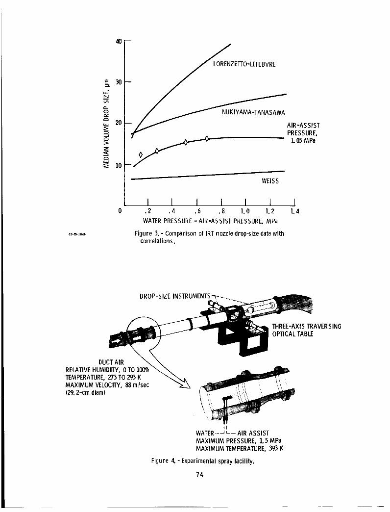
CD-IE,-176Z8
40
30
20
_ 10
m
EI-rO-LEFEBVRE
-- _AIR-ASSIST
_PRESSURE,
_,_,_ 1.05MPa
WEISS
I 1 I I I I.2 .4 .6 .8 1.0 1.2
WATER PRESSURE -AIR-ASSISTPRESSURE, MPa
Figure3.- ComparisonofIRTnozzledrop-sizedatawithcorrelations.
I1.4
DROP-SIZE INSTRUMENTS
THREE-AXISTRAVERSINGOPTICALTABLE
DUCTAIRRELATIVEHUMIDITY,0 TO 100_TEMPERATURE,273TO 293KMAXIMUM VELOCITY,88 m/sec(29.2-cm diam)
\i1
WATER-_ "- AIR ASSISTMAXIMUM PRESSURE,1.5 MPaMAXIMUM TEMPERATURE,393K
Figure 4. - Experimental spray facility.
74

ORIGINALPAGE ISOF POORQUALITY
PRINCIPLEOFDIFFRACTIONSIZING
m ,_wmm_mlm, l# ibl _vw_,Q im D_V,CON_ e B,w_ w,p
SMALLPARTICLESDIFFRACTLIGHTTHROUGHLARGEANGLESANDLARGEPARTICLESTHROUGHSMALLANGLES
WHENA FOURIERTRANSFORMLENSIS USED, THELIGHTDIF-FRAClEDBY PARTICLESOFAGIVENSIZEAT ANY POSITIONIN SPACEALWAYSFALLSONTHESAMEPARTOFTHEDE-lECTOR
Figure 5.- Malvern sprayanalyzer.
. _.\'.._/_,":._:.,_ .; "..'.-:,;,'-.-;",:*;:..:'P=..-,....
.,-;., ,. _ ,..,...,.....;..:,_,. ":';: ,_, ....
......¢::,......._',.....;.,...,.:.._...,.......
:...._...: . :'.:. .. ,.:... ._...:.;_,.... ". :,,.._.',,,,,.• ,. ,"_'. ;." "_ • ";_, . ,'.* "" "_" ""..:" . st ";: ,'".
• : , ......; ". :......." ._._...., :.;",".!.o" _. .._. , .. ..' ,:_.:" ":T.. ".'.'_' :( ".'.'*_.'._." "';_,'...''_'" _" "_"':'>'" "_ '/"" .-'. . " ",: w.';_ _" "°..,;:"." "; ,_";"'_..
-;''.." ,'_""w'.,_,;"i • ", .,( '._' "_. :.; _ ,'_.'..• .,,,. , .'...,_ :_,,_.._','..",, t." .. ;- ' :.. ''._- _.. •o,....; _ : .. , .._° • .. _., _",;° _ i_ ,o.. _. :,' .._ _,. , •
,.,-.._.,...,.. ..¢ ...,.;.... .... .,,......,...,-.....".¢
_..,;. _..... ,....'_,..:.: ......,p..,..'.." ;_.,,',.P.."....,...'_:. • ._.,...,._, .w'_?,.: ._ ..,.;..;,, _'...:."......_.
• ...,,• ...'.t ._ ._ ,. ".'t,'_'4 ' • , '_':..,_.-.,: _'_. "( ' ,
• ...","1.'.-';; ,;" •."-'_ I. f - • ;" f"'" , ._ ,_."_'.
• -..,'.,;-.,...,..2*.,; .......,.:
•", ... ,'.:';._...,,,,,'_,.'._c..,,r-_._..._" -,,Z .'" _,.,- ,r .. • "; _. _,"
•, _. __._ ... .;_ _" _ .'.:'.. ,_."•
"_ ;'.', 4 ... "-'.' " "# %,•.:..,'._:;,,":..,_.
Figure 6. - Photograph of sampleareaand quality control array of Hirlemancalibration reticle (RR.-50-3.0-0.08-102-CF-#115). Magnification 10x.
75

Jr WIDE-ANGLEREFRACTION
D "_ THROUGHDROP, CAN BE
._._@ NEGLECTED
_, _ ¼ MEDIUM-ANGLEDIFFRACTION..... AROUNDDROP, B= _/TrD,
"_r"_---'_--4F MEASURED
____ SMALL-ANGLE DIFFRACTION
NEAR ENVELOPEOF LASER BEAM.PREVENTS MEASUREMENT AT
SMALL ANGLES
Figure 7. - Three principal componentsof scattered light at test section.
CD-IB-IT_7
CD 85-17413
>c
C/3
ZI.i.II--Zi
"1-c_
X
lo"-; 0
_D r- DIFFRACTIONNEAR
// ENVELOPEOF LASERBEAM
DROP
(a) Light intensity as function of light-scatter angle.
MEASUREDINTERVAL
I., _1
BMEASURED
LIGHTSCATTERANGLE,B
(b) Product of light intensity and light-scatter angleas function of light-scatter angle.
Figure 8. - Intensity of forward-scattered light.
76
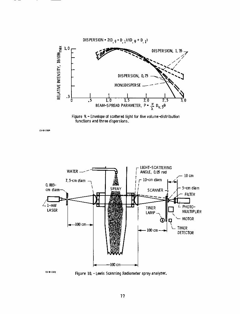
CD-85-17629
DISPERSION- 2(D.9" D.I)I(D.9 + D.i)
._ 1.0 DISPERSION,1.35 .7
0 .5 1.0 1.5 2.0 2.5 3.0
7rDv"5BBEAM-SPREAD PARAMETER, P- _.
Figure 9.- Envelopeof scatteredlight for five volume-distributionfunctions and three dispersions.
I
7.5_m diam --_ Io.oo3- Icm diam--. _ 131_.| _Y
LIGHT-SCATI'ERINGr ANGLE,0.05 rad
F lO-cm diam z/-- lOcm
I I SCANNER- 5-cm diam
I ... _TER
-._l_i_ F. 1 L_ PHOTO-t--_ MULTIPLIER
"_- MOTOR
.,F-- 100cm_ _-- TIMERDETECTOR
C0-_-17632
100cm =
Figure 10. - Lewis Scanning Radiometersprayanalyzer.
77
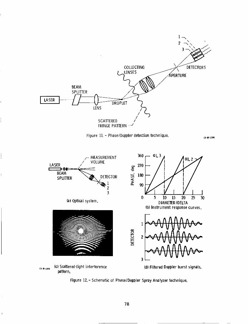
l LASER
\
2 --x\
COLLECTING _ DETECTORS
_._SE__ "_ERTuRE
LENS I/'-'_// "-)
SCAI-IERED IFRINGEPATTERN--Y
Figure 11. - Phase/Doppler detection technique.
/- MEASUREMENT/ VOLUME
LASER /
ECTOR
3
(a) Optical system.
360
270
_" 180(._
-r
a_ 90
-- ¢)13. . .,,
"/i A°'_J7-II I> I
5 10 15 20 25 30
DIAMETER/DELTA
(b)Instrumentresponsecurves.
CD-_,-17631(c) Scattered-light interference
pattern.
e,,,0I--oi.l,.II--1.1.1
r,_
..,,AAAAAA^ ,,""vvvvvvv-,,^AAAAA^,,_"" vVVVV vv"_.,^A A AA Ate,,-- v _/ Iltl tlllU vv"
" vvvv"
(d) Filtered Doppler burst signals.
Figure 12. - Schematic of Phase/DopplerSpray Analyzer technique.
78

_ DEPTH-OF-FIELDCHECK
/P DUMP SPOT _K
iIiZ_NtNj<IODE X-BEAM SPLITTER DLVMP_SSPoTl__%,//_
PARTICLEPLANE-- -- _I _
CONDENSINGLENS _
HELIUM-NEONHYBRID LASER
Figure 13. - FSSPoptical path.CD-85-17_
>,..
z
zi
104
103
io2
E
E
i
mmE
i
i
101 -_--m
i
m
lOo --
D
10-110-1
I , I i l,l,l I i I ,lJlll I , I ,I,I,I
I0 0 I01 102DROPSIZE. IJm
Figure 14.- Forward-Scattering Spectrometer Probe(FSSP)light scattering as function of drop size. Light intensitymeasuredat scattering angles of 40 to 140.
CD-_-lFJql
79

COLLIMATED 11
LIGHTBEAM _
VIEWING _ _ !!!iVOLUME -- ""._. i;.,/i
>%,'
AREA ,_BY A_
Figure 15.- Optical Array
SAMPLINGAREA
FLIGHT
"K:_::> DIRECTION
F SAMPLED/ VOLUME
O
ID
\k.___INTERMEDIATESHADOWPLANE
Probe (OAP)operating principle.
>2. O-mWHELIUM-NEONLASER
SECONDARYZOGMLENS
PHOTODIDEARRAY
@CONDENSINGLENS; F- 320 mm
MIRROR
MIRROROBJECTIVELENS; F- 60 mm
Figure 16.- Optical Array Probe (OAP)opticalpath.
8O

\ EDDY 4f\ _" DROP PATH
\\A_"_ / MEAN PARTICLE
(_,. _ X_........ _VELOcITY,Up
/ _ \\ PHASE VELOCITY,
EDDY PATH
Figure 11.- Phase interactionsfor particle-laden flow.
I
+ u p)i
Figure 18.- Locally homogeneousflow (LHF)model.
81

ASSUMPTION: FINITEINTERPHASETRANSPORTRATESBUTPARTICLESONLYRESPONDTOMEANMOTION
!
/-(u+u )i/
/ ! --
i_- (Up + u p)i" Upi#Ui
NOTES: I - PARTICLEDISPERSIONIGNORED" ONLYVALID FOR"LARGE" PARTICLES
II - MOSTWIDELYUSEDAPPROXIMATIONIN CURRENTMODELSOF COMBUSTINGSPRAYS AND PULVERIZEDCOAL
III - FLOWFIELDFOUNDFROMEULERIANCALCULATIONWITHDISTRIBUTEDSOURCETERMSDUETO PARTICLES. LAGRANGIANCALCULATIONDETERMINESPARTICLETRAJECTORIES
Figure 19.- Deterministic separatedflow (DSF)model.
CO-_-IT_
0
i -1,j
k+l III
TYPICAL PARTICLE
CLASSTRAJECTORY
i,j+l
i
II
).. I
II
i,j-1
Figure 20. - Gas-flow computationalcell.
(3-i+l,j
CO-_ IT4m
82
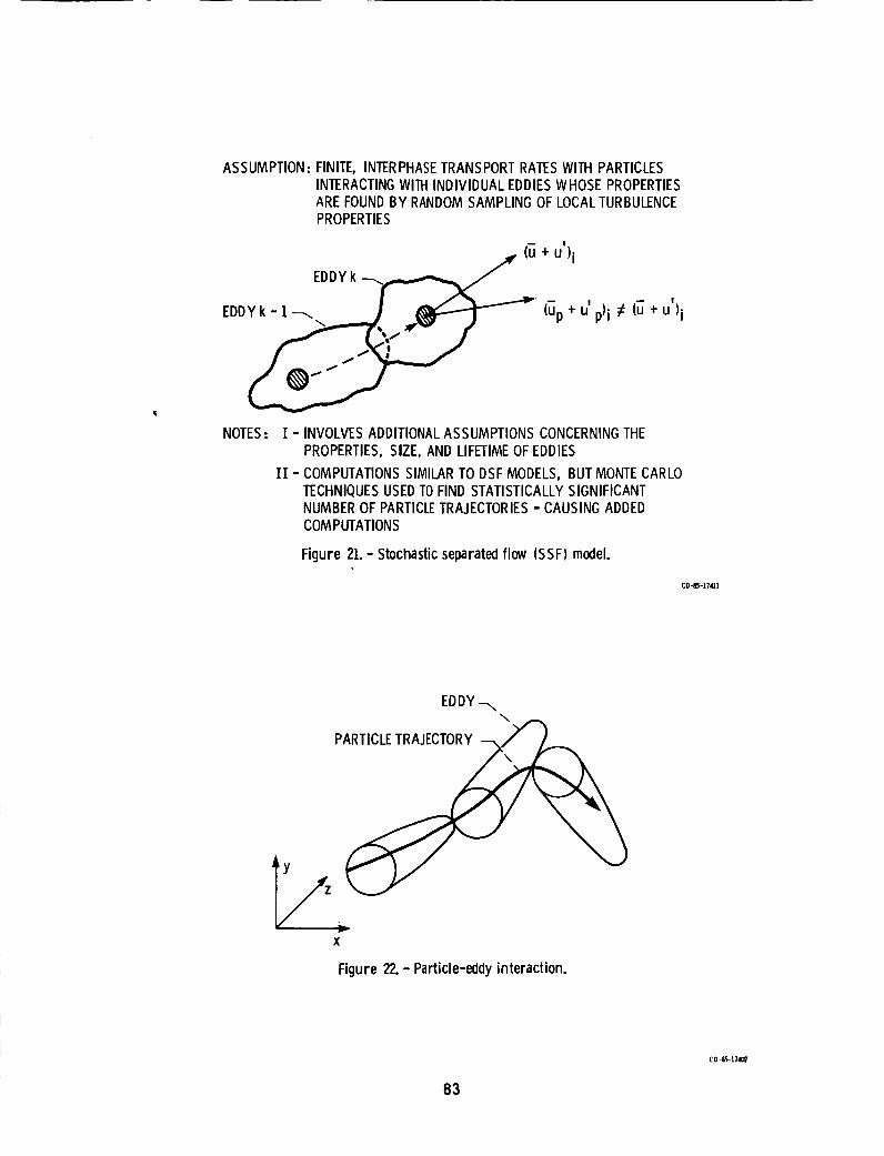
ASSUMPTION:FINITE, INTERPHASETRANSPORTRATESWITHPARTICLESINTERACTINGWI1HINDIVIDUALEDDIESWHOSEPROPERTIESAREFOUNDBY RANDOMSAMPLINGOF LOCALTURBULENCEPROPERTIES
EDDYk
I
(u + u )i
EDDY k - 1 (Up + u' p)i _ (_ + u')i
NOTES: I - INVOLVESADDITIONALASSUMPTIONSCONCERNINGTHEPROPERTIES,SIZE, AND LIFETIMEOF EDDIES
II - COMPUTATIONSSIMILARTO DSFMODELS, BUTMONTECARLOTECHNIQUESUSEDTOFIND STATISTICALLYSIGNIFICANTNUMBEROF PARTICLETRAJECTORIES- CAUSINGADDEDCOMPUTATIONS
Figure 21.- Stochastic separatedflow (SSF) model.
C0-_-17411
EDDY--_\
P
Y
/zX
Figure 22. - Particle-eddy interaction.
C0-85-1N07
83

..,.,.,
I=
>c
c_o
I.i,.I
..J
X
z
W
_E
28
24
20
16
12
B
EXPERIMENTAL,xld
o 50A 100o 2.50 o0 60O
THEORY
SSF
DSF0 0 ....
0
0 0
o xld
-- _ lO0
0 ////" A. Z_
'7-_ o I/ f/J 250
_ L/A A ///_//o
/
_-- _ 600
I I I I I I I I I I40 80 120 160 200
DROPDIAMETER,pm
Figure 23.- Mean axial-dropvelocitiesalong axis. Non-evaporatingspray; case2.
84

1.00
•75
.50
.?_5
0
D
n
m
00
0
THEORY
SSFDSFU-IFEXPERIMENTAL
0
00
0
I I I I I °l ol(a)xld - 50.
1.00
•75
• 50
to 0d (b) xld - 100.
<c 1.00_
X-', .75
•25 _"'_,,
o I I(c)xld - 250.
1.00
.751- "t, o.,0I-- !N. o
•"P I I I I0 .04 .08 .12 .16 .20 .24
RATIOOF RADIALTO AXIALDISTANCE,rlx
I• .28
(d)xld - 600.
Figure 24. - Radialvariation of mean liquidflux. Non-evaporatingspray; caseL
85

100
8O
60
4O
20
0
E.m
c 80I=
60¢U
THEORY EXPERIMENTAL
SSF 0 CASE i
__ DSF 0 CASE 2
__ 0 O''"-'_ .... "
I II I I I I
(a) Nonevaporatingsprays.
40
20
04
--0-
m
I I I I I I60 80 100 200 400 600
AXIAL LOCATION,x/d
(b) Evaporatingsprays.
Figure 2.5.- Sauter mean diameter (SMD)along axis.
86

LDASENDINGOPTICS--X
MOVABLESCREENEDENCLOSURE--_%.
INJECTIONTUBEWITH ,__ _x_AXIALTRAVERSE-----..__
I
/-- LDA RECEIVINGOPTICS
I -- MINICOMPUTERII F TERMINALI, [2l-
\2-W ARGON-ION LASER--_
I r
_',,,_\\\\\\\\\\\ ",:,\-:,\ _/
ENCLOSURETRACK /(X-YTRAVERSE) --/
i _ I /- COUNTER/ _ I -
==L ._=:IEI_F_r_-l-l--l_
•-" / Iq ' .I I. , / rms \
,_"_7_\__\,_,_'_\/_\\_/ VOLTMETER _OSCILLOSCOPE-_ /
/ /---INTEGRATINGDIGITAL/- PARTICLE- VOLTMETER
LADENJET
Figure 26.- Particle-laden swirling-flow experiment.

N87-20273
COMBUSIION RESEARCH ACIIVIIlES AT THE GAS TURBINE RESEARCH INSIlIUIE
Shao ZhongpuGas Turbine Research Institute
Jiangyou County of Sichuan, People's Republic of China
The Gas Turbine Research Institute (GTRI) is responsible mainly for basic
research in aeronautical propulsion. The combustion research activities pri-
marily cover the following areas: annular diffuser for the turbofan augmentor,
combustor ignition performance, combustor airflow distribution, fuel injectors,
vaporizer fuel injector, and airblast atomizer.
RESEARCH ON THE ANNULAR DIFFUSER FOR THE TURBOFAN AUGMENIOR
It is well known that the inlet velocity profile has a very strong influ-
ence on diffuser performance. The inlet velocity and temperature profiles are
not uniform: both change with flight condition. The diffuser enlarges the
inlet velocity distortion; that is, the nonunlformlty of the velocity increases
with the diffusion process occurring in the diffuser. The nonuniform inlet
velocity profile encourages the alrstream to separate from the diffuser wallor inner cone, induces flame stabilization in the separated flow region, and
causes augmentor components to burn or to induce combustion instability, lo
obtain a desirable fuel-alr distribution, it is necessary to understand the
velocity and temperature profiles in the augmentor. In other words, since the
velocity and temperature profiles at the exit of the diffuser must be known
some experimental research was carried out on the annular diffuser of the tur-
bofan augmentor.
The test model and the instrumentation locations are shown in figure I.
The test was run at the following cond_tlons:
(I) Inlet Mach number, 0.08 to 0.60
(2) Inlet temperature, 300 to 600 K(3) Inlet Reynolds number, >SxlO 4
(4) Diffuser outlet to inlet area ratio, 1.54
(5) Inner to outer annular area ratio, =l.O
(6) Inner cone, three configurations
(7) Cone angles, 20°, 30°, and 40°
The statlc-pressure recovery coefficients, velocity proflles, and temper-
ature profiles along the axial distance were measured. The flow separation inthe diffuser was studied by tuft observation method for low-temperature airflow
under different inlet outer-lnner velocity ratios and different Inner-cone con-
figurations. Typical inlet velocity and temperature profiles of the diffuser
are shown in figures 2 and 3.
We found the following results:
(1) Within the range of the test Mach number (Mi or Me < 0.6), the
statlc-pressure recovery coefficients at different axial stations were indepen-dent of Mach number. As shown in figure 4, the inlet Mach number had little
influence on the diffuser internal flow. Thus, the effect of inlet Mach number
89
C -_- _E_G P_E _ NOT FILMED

can be neglected when testing or analyzing the performance of an annular dlf-fuser for a turbofan augmentor.
(2) We also obtained an important nondimenslonal flow parameter,
=-V2 --2(Ve e05)(vi iO:If we use a diffuser with the same geometry and a similar inner velocity
profile and maintain SD = constant, then the change of statlc-pressure
recovery coefficients and nondlmenslonal, combined veloclty-temperature combi-nation distributions along the diffuser axial distance is the same, regardless
of whether the test is done with low- or hlgh-temperature air, as shown infigures 5 and 6. It is possible to use the low-temperature test to simulate
real turbofan augmentor diffuser flow; low-temperature airflow separation canalso be used to understand hlgh-temperature airflow separation.
RESEARCH ON COMBUSIOR IGNIIION PERFORMANCE
Under the hlgh-altltude rellght condition, the combustion chamber inlet
pressure can be as low as 0.2 kg/cm2, and the inlet temperature can be as
low as -50 °C. Because it is important for combustion engineers to understand
the relation between ignition performance and combustor inlet parameters, we
studied the effect of inlet parameters on the ignition performance of combus-
tors with different fuel-injectlon systems.
This test was performed on the hlgh-altltude ignition test rig shown in
figure 7. Three combustor configurations were used. The first configuration
was a gas turbine combustor with a pressure swirl atomizer. (This combustor
is similar to a JT-3D engine combustor with one flame tube.) The second con-
figuration was a one-quarter sector of a full annular combustor with three
T-shaped vaporizers, as shown in figure 8. The third configuration was similar
to the second one - the only difference being that the three vaporizers hadbeen replaced by three alrblast atomizers.
A hlgh-energy ignition plug was used for every configuration. The stored
energy of the ignition system was 20 J, 12 J, and 8 J, respectively. The igni-
tion procedures were repeated three times under every test condition. If all
three ignitions were successful, then each was Judged a successful ignition atits specific condition.
We drew the following conclusions from this experiment:
(1) The inlet pressure has a significant effect on the ignition perform-
ance of the combustorso Figure 9 shows the optimum fuel-air ratio as a func
tlon of inlet pressure for the three configurations. From figure 9 we can see
the effect of the inlet air pressure on ignition performance of the combustors,especially at low pressure.
(2) The inlet air temperature has a strong effect on the ignition perform-
ance of the combustors. The effects of the inlet air temperature on maximumignitable reference velocity and on optimum fuel-alr ratio for the three con-
figurations are shown in figures lO and II. As the inlet air temperature
decreases, the maximum ignitable reference velocity decreases. At higher inlet
90

air temperatures, the effect of the Inlet atr temperature on the optimum ignit-able fuel-air ratio Is very weak; however, at lower inlet alr temperatures theeffect is very strong, especially for the vaporizer combustor.
Figures 12(a), (b), and (c) show the combined effects of inlet air pres-sure and temperature on ignition performance for the three conflgurations.
EXPERIMENIAL STUDY ON AIRFLOW DISTRIBUTION OF THE COMBUSIOR
The airflow distribution characteristics of a combustor directly affect
the performance of the combustor such as combustion efficiency, range of sta-
ble operation, and temperature profile at the combustor exit. A 90 ° segment
of the annular combustor was used for this study. The test assembly Is shownin figure 13.
The goals of the study were as follows:
(1) To determine the effect of Mach number at the combustor inlet on the
airflow distribution at an alr temperature of 291 K(2) To compare the changes of airflow distributions wlth and without
burning in the combustor
Figure 13 shows the eight instrumentation sections on the test assembly.
The flow rate Ghl through the holes on the wall of the flame tube can becalculated as follows:
where
Cdl
Ahl
Y
Ap
Ghl = CdlAhl 2_ AP
airflow discharge coefficient of the holes
area of the holes
specific gravity of alr
pressure drop through the holes, = Pal - Pll
acceleration of gravity
The flow rate (In percent) through each row of holes that is relative to thetotal is
Gi = lO0 hi Ghl
The relative area (In percent) of the holes of each row of holes is
AI = I00 hl Ah
91

The following conclusions were obtained from this experimental study:
(I) At the range tested, there is no apparent influence on the airflow
distribution by the Mach number at the combustor inlet, as shown in figures
14(a) and (b).
(2) Under the conditions
1 = 291 Kin
*/l*lex in = 1 N 2.44
the airflow distributions have no obvious change, regardless of whether burning
is present or not, as shown in figures 15(a) and (b). However, we are not
certain that this would be true under real operating conditions.
EXPERIMENIAL SIUDY ON FUEL INJECTORS
The fuel injector is one of the most important components of a combustor
or afterburner. In order to determine the effects of geometric parameters,
airflow parameters, and fuel rate on the fuel-spray characteristics, we have
made an initial study of a vaporizer and an airblast atomizer.
lhe test rig assembly is shown in figure 16. The airflow rate Gathrough the fuel injector was measured by a turbine flowmeter. The air veloc-
ity at the injector exit was
Va = Ga(R)T2/AP
The fuel rate Gf was also obtained by a turbine flowmeter where the air-
fuel ratio is given by
AFR = Ga/G f
The Sauter mean diameter (SMD) of the fuel spray drops was measured by a
Malvern laser particle slzer.
EXPERIMENIAL SIUDY ON VAPORIZER FUEL INJECIOR
Since we tried to understand the spray characteristics - not the vaporiz-
ing condition - for different vaporizer fuel injectors, we studied the spray
characteristics under low inlet air temperature only and did not heat the
vaporizer. Some of the test vaporizers are shown in figures 17 and 18.
The following conclusions were made:
(I) The air velocity Va at the vaporizer exit is the most important
factor affecting fuel atomization. As shown in figure 19, SMD decreases with
increasing Va.
92

(2) The effect of air-fuel ratio on fuel atomization is related to theair velocity at the vaporizer exit. If AFR<4 and the air velocity is low,then, as AFR increases, SMDwill decrease. Whenthe air velocity is muchhigher, the effect is not apparent, as shownin figures 20 and 21.
(3) lhe method and the pressure of injecting fuel into the vaporizer hasno significant influence on fuel atomization, as shownin figure 22.
EXPERIMENTALSTUDYOF1HEAIR-BLASTATOMIZER
lhe geometric parameters of the airblast atomizers we have tested arelisted in the following table:
Number
0
II
21
7
17
lO
Inner channelfeature
Straight flow
With swirl vane
Straight flow
Straight flow
Straight flow
With swirl vane
Outer channel
feature
Tangent flowholes
langent flowholes
Rectangularflow holes
Rectangularflow holes
Rectangularflow holes
Rectangularflow holes
Total exit
area,
295.4
295.4
359.5
295.4
235.1
295.4
lhe test atomizers are shown in figures 23 and 24.
The conclusions were as follows:
(1) Under the test conditions, SMD decreased with increasing airsprayvelocity, as shown in figure 25.
(2) When AFR <4, SMD decreased with increasing AFR. When AFR >4, there
was no significant influence on SMD, as shown in figure 26.
(3) For the same conditions, SMD decreased as the exit area of the atom-
izer increased (fig. 27). The reason for such a result has not been determined
yet.
There are many interesting subjects related to combustion such as combus-
for exit temperature profile, the procedure to control exhaust emission, com-
bustor diagnostics, swirl combustion, and cooling techniques. We are prepared
to do further experlmenta] study.
93

6mo
0
0
0
Ii
m
m
m
w
I
./
"_sQ'O
"c;
i
I
i
A9_,¢
iI
\1/'I/
m
a9co
u®_,m
L
E
'10
m
L,
\
o0(3",
m
{}:o"-"-_" .uo
o ,_I c
o
oo
.-I
Q_L
Q_Q)
L,
¢)
¢I
Q_
t,.,
¢I
E
I-0
C0
U0
0
t-O
.f--
o
0JEQ,)
E
o
I,,,_
94

0 oo 0
0 0
,L.
Q)
kJ
,.., r.
0 ,,_0
, I
t_ ",o6d o
0 0 u 0
L
r_
S,-_:_ i
0
4)
El
E6..
[--
C,- cz_ _,, 06 & 6 •
0 0 0
0
cO
,S
0
-d"6
0
Ou
,S
0
0,--
._ .,--0
(1) L..E o-
c-4-_0"_"c" _,j
0
,_:%u
_ C
If,,..
m_
r
0 0
• • D
0 0
E
I •
' w
0 L_ 0 0
%0 I 0-
0 k,, L. 0 •
,,.., .0
•,-" _ ! I
c_o 0 0 --
Q _
S d S d _;0
0
d
3
0
0
L-
c-O
,¢.=.
c"QJE
_.-0
c-
¢,._ p--
I
f%l ,r-U
95
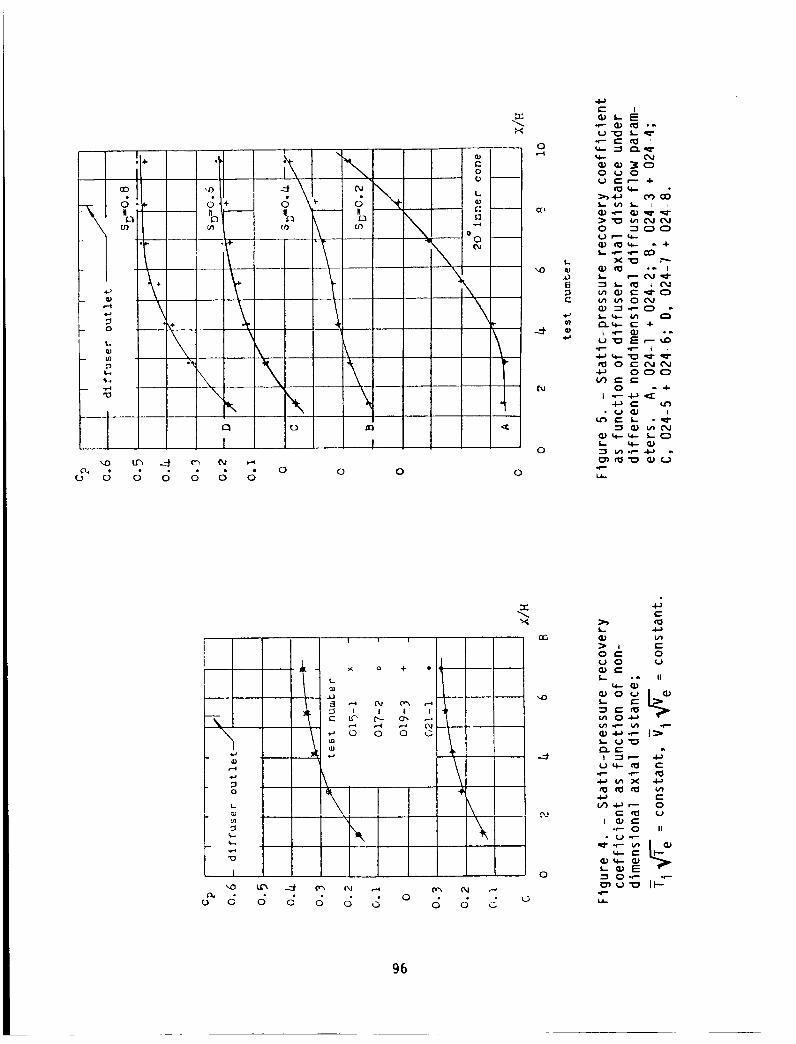
\
e-,
r °
0 .6-
IS)
\
P,
\ \
I
I I
8 G 8 o o 0
ou
L
C:
° 0
\\
X
4
0
0
Ixl
0
L..
r_
el)
Yo
L
I
M_
_ J
!
c- U"
ill
\
J J J J j
! i
r',.- c_,
o _ a
0
\\
J J
• I0 _-¢.J 0Q._ r-$-
=°0
¢'_ e-
(_)_-.,¢.-.
C_.._e"
_2
,,¢..-
X
0
E
.d
0
II
e'-
e-0
II
96
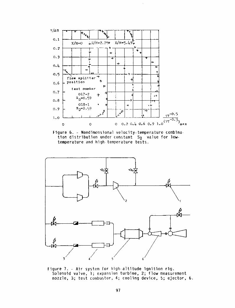
Y/_R ÷%0. i
x/H=o +x/H=__.7_+ xlH-5._9_
o._ I +
0._) {t- 4- _
0.5 +•+ ÷ +
flow splitter "t
0.6 _ posltlon +
test number,+
o.7 - o17-2 + "+ _ .+
0.8 - aD'O" 59 1 + l.i.O18-1 • + .+ .+
0.9 - sDxo-59 ._ [
0 0
wr-°" 5
0 0.2 0._ 0.6 0.9 l.O(VT-O'_)max
Figure 6. - Nondimens_onal velocity-temperature combina-
tion distribution under constant SD value for low-temperature and h_gh-temperature tests.
F2
/3
4
4 5 6
Figure 7. --Air system for h_gh-altltude ignition rig.
Solenoid valve, l; expansion turbine, 2; flow measurement
nozzle, 3; test combustor, 4; cooling device, 5; ejector, 6.
97

Figure 8. Installation of ignition plug in vaporizercombustor. Starting fuel injector, l; high-energyignition plug, 2.
0.12
0.10
0.08
O.06 --o
"3o
c_ 0.04 --
0.02 --
00 2
Figure 9.
_o 0 combustor with pressure swirl atomizer
• combustor with vaporizer
mbustor with air blast ato_dzer
I I I I I I I I I I Io.4 o.6 0.8 1.o 1.2
p_ k_Iom2
Optimum fuel-alr ratio versus inlet pressure; l_ = 293 K.
98

5O
ORIGINAL PAGE IS
POOR QUALII'Y
0 p_=o.46kg/cm2 pressure swirl atomizer
P_=<_.28kg/cm2 pres_-ure _'ir] _tomlz_r
p_=1.5Ok_/cm 2 air bl_st _to_ti_,;_"
p_=_D. 98kg/cm 2 vapcrlzer
I ] I240 260 280
T_ Z
Figure I0. -Effect of inlet temperature on maximum ignitable
reference velocity.
99

0.1
0.10
0.08
O
0.06o
g
0.04
0.02
0
D "1_ ,Y2=O.62,:g/cm2 [,rsssure swirl nto_Azer
O P2--0.28kg/cm2 pressure swirl atomizer
A P_= 0.98kg/cm 2 vaporizer combustor
[] P_=1.30kg/cm 2 combustor with air blastatomizer
II IIZ_k
2r
I i i I i i i i220 230 240 250 260 270 280 290
T_ K
300
Figure II. - Effect of inlet temperature on optimum fuel-alr ratio.
I00
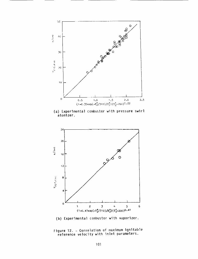
5O
L_
4O
3O
=.
20
10
0
0.5 1.0 I,5 2.0
* " " 0(1-43._Sex]D(-T2/310)/P2) (T2-200 ) •22
2.5
(a) Experimental combustor with pressure swirlatomizer.
24
>
2O
16
12
0
(b) Experimental combustor with vaporizer.
Figure 12. - Correlation of maximum ignitable
reference velocity with inlet parameters.
lOl

7",C_6
24
2O
16
12
O _ .O 2.0 3 .o
(I-O•?Ie_"p(-T_/3IO)/P_)(T_-200)0"_O
(c) Experimental combustor with air-blastatomi zer.
Figure 12. - Concluded.
2 3 4 5 0 7
1,1SV'
_-,1----_,
U
I
I ,
8
8
2' 3' 4' 5' 6' 7'
Figure 13. - Test combustor and instrumentation on locations.
102

ORIGINAL P_%GE ;S
OF POOR QUALITY
1.0
0.8
0.6
0.4
0.2
O.OC
_ 22
0.2 0.4 0.6 0.8 1 .G
(a) Outer annulus.
1"2
_.0
0.8
.3.6
0.4
0.2
O. OC
//
O ['i2 = _a" _-_
• 0.32
A =-#-z7
I 1 I0.6 O.8 I .0
(b) Inner annulus.
Figure 14. - Effect of Mach number on air-flowdistribution of annulus; lin = 291 K, Tex/Tin = I.
103

2.44
I I I I t0.2 0.4 0.6 0.8 _ .0
7
(a) Outer annulus.
o T /Tin ,, I .00ex
• 2.44
o.o I I I Io._ o.4 o.6 0.8 _.o
(b) Inner annulus.
Figure ]5. - Effect of combustion on air-flowdistribution of annulus.
I04

Air _:
' Fuel
• _-i-_ ._m'_ - Movable window
tMalvernI, 2200J !
Air
Exhaust
\Type printer
Figure 16. - Test rig assembly.
I05
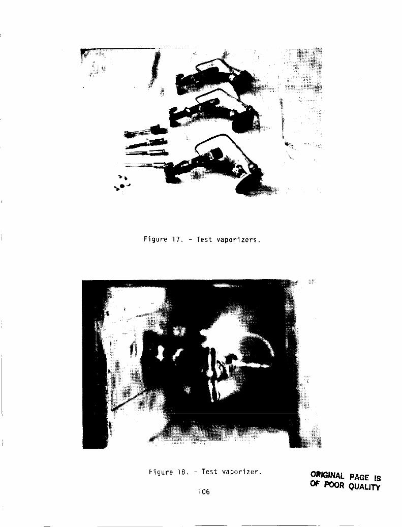
Figure 17. - Test vaporizers.
Figure 18. - Test vaporizer.
I06
ORIGINAL PAGE IB
OF POOR QUALITY

l-
t C3 (-)
W7_
/1 I I 1 I 1 I
O O O O O O O O
rll
O
( _'__) _l;I ,_;
0
V_
0°r- 04--_l,l'l
i- Ii
,---_(I#
,_- I.
°r--#4-_ l-"
°_
I.I.I--I
II-
•N
I-- I_.
°_I.I..
OO_
,D O'l',_ O',O
o c_- _ -_
1 1 I I l I IO O O O O O O
I0
0
__ 0
-- 0
c-O
o_
e,-
o
i._ I'i
NI °r--
_..• 0
_.
L _-
_'_ u_.°tin
107

0 GO u'_ _ 0 0
• g c; c_ _ - _11_,_
_ ,_" _ ._- .- _0fa//J
o • 1_ --
_ -
I I I I I I I0 0 0 0 0 0 0
( _ _') (1WS
0
0
0
0
0
o_E
o E
"I_0oL.r_l-
-I-I II
E.-.J
l.-,e-I x
0O
0Ii
_,- x'.-i.-
I I I I I 10 0 0 0 0 0
{0 _ '.43 L_
( _ _) cll..If:
r_
i "/o
I 1
0 0
q
/
1_' [
0
Lf_
O"
k.0
o E
O0°_-
_.1
:_OJ
L _.f- ¢__ 0
O _°r"_
._ e-
_,.r--
i
£-
e"- MC'_ °r-
_ O
°r'-
108

ORIGINAL PAGE IS
OF POOR QUALITY
%
Figure 23. - Test air-blast atomizer.
Figure 24. - Test atomizer.
lOg

"_t_u",sr_ b oot_L_ kO
!
Do
I I I I 1 l
0 0 0 0 0 0
-- Lf',
O,J
L.
0
t-
O
0
"-t=_ E
r"- C'_
I --J
f,-
"_ ,._¢...-
O
•_ <3)
c._ N
_ .e.-
I
t_ r---
12
I I I I I I
_ 0
__ 0
-- 0
-- 0
0
0 0 0 0 0 0
(m_) _S
ill
_>
f,-
0
0
+-_ EE
"_ _0
-.J
0
N
°r-
E
u+- 0
I
0_1 r-"
"1 *1-"
_rO-r'-
110

6O
5O
4OE
Em 30
20
I0
\
1 i l J
dO 50 60 70
V (m/s )a
Figure 27.-- Effect of nozzle outlet areaon SMD; AFR = 2.5.
III
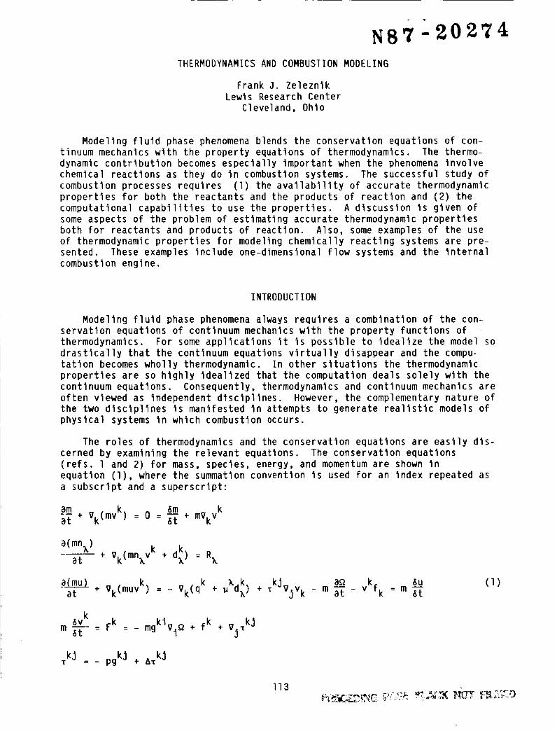
N87-20274
THERMODYNAMICS AND COMBUSTION MODELING
Frank J. Zeleznlk
Lewis Research Center
Cleveland, Ohio
Modeling fluid phase phenomena blends the conservation equations of con-
tinuum mechanics with the property equations of thermodynamics. The thermo-
dynamic contribution becomes especially important when the phenomena involve
chemical reactions as they do in combustion systems. The successful study of
combustion processes requires (1) the availability of accurate thermodynamic
properties for both the reactants and the products of reaction and (2) the
computational capabilities to use the properties. A discussion is given of
some aspects of the problem of estimating accurate thermodynamic properties
both for reactants and products of reaction. Also, some examples of the use
of thermodynamic properties for modeling chemically reacting systems are pre-
sented. These examples include one-dlmenslonal flow systems and the internal
combustion engine.
INTRODUCT ION
Modeling fluid phase phenomena always requires a combination of the con-
servation equations of continuum mechanics with the property functions of
thermodynamics. For some applications it is possible to idealize the model so
drastically that the continuum equations virtually disappear and the compu-
tation becomes wholly thermodynamic. In other situations the thermodynamic
properties are so highly idealized that the computation deals solely with the
continuum equations. Consequently, thermodynamics and continuum mechanics are
often viewed as independent disciplines. However, the complementary nature of
the two disciplines is manifested in attempts to generate realistic models of
physical systems in which combustion occurs.
The roles of thermodynamics and the conservation equations are easily dis-
cerned by examining the relevant equations. The conservation equations
(refs. l and 2) for mass, species, energy, and momentum are shown in
equation (1), where the summation convention is used for an index repeated as
a subscript and a superscript:
a__m 6m kat ÷ Vk (mvk) = 0 = _-_ ÷ mvkv
a(mnx)at ÷ vk(mn_vk ÷ d_) = R_
+ vk(muv k) qk ), k TkJvj a_ vkfk 6u (1)at = - Vk( + _ d}) ÷ vk - m _ - = m _-_
6vk Fk fkm _ : = - mgklvl_ + ÷ Vj_ kj
kj pgkJ 8kJT : - ÷
ll3• _ __'l_ _,Cr_

In these equations, m is the mass density, u the internal energy per unitk k
mass, nx the moles per unit mass of species x, v the velocity, q thek
heat flux, _ the chemical potential per mole of species x, d_ the dlffu-
sive flux of species X, and Rx the volumetric rate of production of species k.In the momentum equation, gkl is the metric tensor for three-dlmenslonal
space, Tkj is the stress tensor, _ is the potential energy, and fk representsall volumetric forces over and above those produced by the stress and the
potential energy. The stress tensor is composed of a contribution from the
pressure p and the dissipative stresses. The symbol t represents time,
vk is the covarlant derivative with respect to the spatial coordinates, and
b/at = a/at • vkvk is known as the absolute, substantial, or convective
derivative. The thermodynamic property functions for pressure, internalenergy, and the chemical potentials are shown in equation (2). These prop-
erties may be regarded as functions of mass density, temperature T, and moles
per unit mass of the species:
p = p(m,l,n),)
u : u(m,T,nx) (2)
,x = _)_(m,l,n_)
Substitution of the thermodynamic internal energy function into the con-servation equation for internal energy converts it into an equation for the
temperature, and the resulting equation now contains explicit contributionsfrom changes in composition and mass density. In reacting fluids the temper-
ature largely reflects the energy released or absorbed by chemical reactions.
Thus, we see that the thermodynamic property of internal energy determines the
temperature and, consequently, the amount of energy released or absorbed. Ofcourse, the temperature, in turn, strongly affects reaction rates and other
physical properties of the reacting fluid. The thermodynamic pressure equa-
tion (an equation of state) appears in the equation for the conservation of
momentum and thus helps to define the local flow field. Clearly, the success-
ful modeling of combustion processes requires two ingredients: (1) accurate
thermodynamic properties for both the reactants and the products of reaction
and (2) computational capabilities to use the properties in modeling combus-
tion systems.
I shall briefly describe some aspects of our work on the two topics of
property estimation and property utilization. First, I shall discuss the
estimation of free radical properties in the ideal gas state and the properties
of nonideal solutions. Following the dlscuss_on of properties, I shall illus-
trate some of our computational capabilities to use these properties to model
the physical systems in which reactions take place.
ESTIMAIION OF FREE RADICAL PROPERTIES
Free radicals are highly reactive species which are usually present at low
concentrations in chemlcally reacting systems. These species play an importantrole in the chemical reaction mechanisms of combustion, lhey are involved in
both the endothermlc (heat absorbing) in_tlatlon steps of the mechanism and the
exothermlc (heat releasing) recombination steps. Recently Bauer and Zhang
(ref. 3) and others have conjectured that free radicals are also important
114

species in the mechanismof soot formation in hydrocarbon flames. Hence, thethermodynamic properties of free radicals are of considerable interest.Unfortunately, relatively little is knownabout the thermodynamic properties
of radicals over the extended temperature range encountered in combustionsystems. Hence, we have found it necessary to estimate the thermodynamicproperties of the phenyl, phenoxy, and blphenyl free radicals which are likelyto be important species in the combustion of hydrocarbons and in soot forma-tion. Becauseof their low concentrations and becausemost combustion processestake place at relatively low pressures and high temperatures, it is usuallyadequate to estimate free radical properties in the ideal gas state.
Thermodynamicproperties for any species in an ideal gas state can beestimated from the canonical partition function using the formulas of statls-tlcal thermodynamics. This requires knowledgeof the species' molecularstructure, its vibrational and rotational energy levels, any barriers tointernal rotation, and the standard state heat of formation. The difficultyis that this information is seldom available for free radicals. As a resultit becomesnecessary to estimate these data from similar, stable species whosemolecular properties have been measured, l hese stable, related species arecalled the parent species of the radicals. The species benzene, phenol andblphenyl are suitable parent species for the radicals phenyl, phenoxy ando-blphenyl, respectively. The relation between these parent species and theradicals is shownin figure l. This estimation procedure is based on the workof Forgeteg and Berces (ref. 4). In this method it is usual to assumethat thebond lengths and bond angles of the radical are identical to those of the par-ent. Also the radical's vibrational frequencies are taken to be the sameasthose of the parent molecule except that three frequencies are eliminated foreach atom which appears in the parent molecule but not in the radical. In somecases, where additional information about the radical is available, the assumedstructure and vibrational frequencies can be adjusted to take into account thisextra information.
Oneof the difficulties with this method of estimation is the selection ofthe appropriate frequencies for elimination. The reason for this is that amolecule's frequencies correspond to vibrations of the molecule as a wholerather than vibrations of a particular bond. Naturally this introduces someuncertainty into the resulting properties. To ascertain the degree of uncer-tainty one might try eliminating different frequencies or, perhaps, perform theestimation with a different parent species.
Comparisonsof the results of our estimation of phenyl and phenoxy prop-ertles (ref. 5) with estimates madeby Benson, et al. (refs. 6 and 7) are shownin tables I and II for entropy and heat capacity. Our estimation of the phenylproperties from benzene and phenol agree surprisingly well wlth each other andwith the room temperature values estimated by Benson. Our estimates of thephenoxy properties estimated from phenol also agree very well with Benson'sestimates which, for this species, were available over an extended temperaturerange.
NONIDEALSOI_UIIONMODELS
The properties of fuels and oxidizers must be accurately known if com-bustion processes are to be modeled properly. Since reactants, especiallyfuels, are often multlcomponent, nonldeal, liquid solutions, it is desirable
115
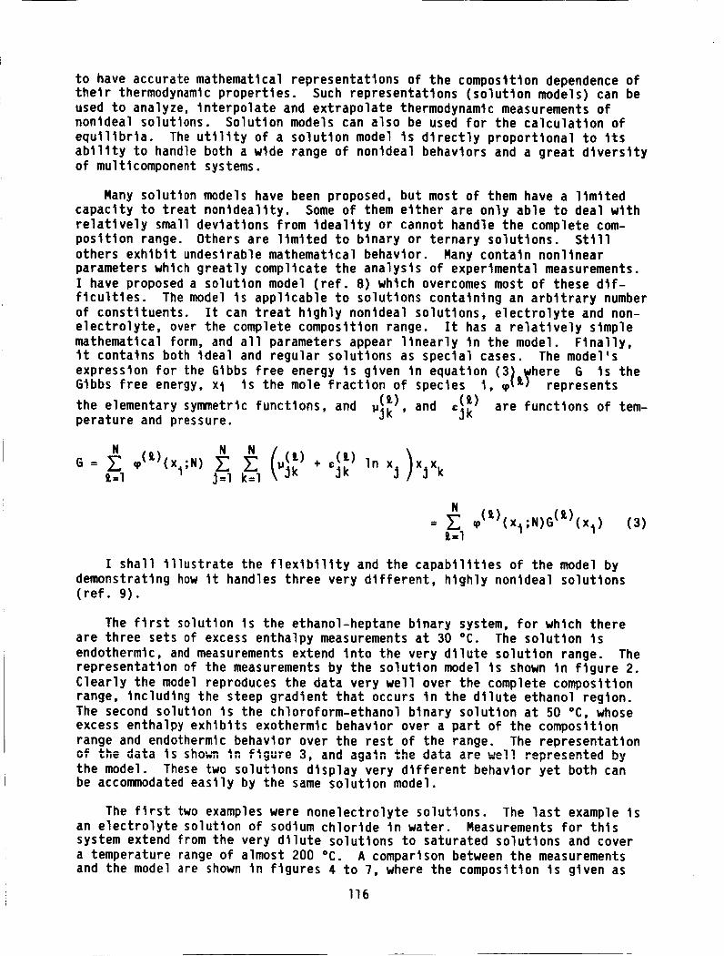
to have accurate mathematical representations of the composition dependence oftheir thermodynamic properties. Such representations (solution models) can beused to analyze, interpolate and extrapolate thermodynamic measurements ofnonldeal solutions. Solution models can also be used for the calculation ofequilibria. The utility of a solution model is directly proportional to ttsability to handle both a wide range of nonldeal behaviors and a great diversityof multlcomponent systems.
Many solutton models have been proposed, but most of them have a llmttedcapacity to treat nonldeallty. Some of them either are only able to deal wtthrelatively small deviations from tdealtty or cannot handle the complete com-position range. Others are limited to binary or ternary solutions. Stillothers exhibit undesirable mathematical behavior. Many contain nonlinearparameters which greatly complicate the analysis of experimental measurements.I have proposed a solution model (ref. 8) which overcomes most of these dif-ficulties. The model ts applicable to solutions containing an arbitrary numberof constituents. It can treat highly nontdeal solutions, electrolyte and non-electrolyte, over the complete composition range. It has a relatively simplemathematical form, and all parameters appear linearly in the model. Finally,It contains both ideal and regular solutions as special cases. The model'sexpression for the Gtbbs free energy Is given in equation (3) where G ts theGtbbs free energy, xt Is the mole fraction of species 1, _(t) represents
(t) and ._)) are functions of tem-the elementary symmetric functions, and gJk 'perature and pressure.
" )G = t_ 1 _(t)(Xl;N) _ _ / (t) + (t)In xj xjx k= _=l k=l _)k =3k
N
t=lq_(t) (x t ;N)G(t)(xt) (3)
! shall illustrate the flexibility and the capabilities of the model bydemonstrating how It handles three very different, highly nonldeal solutions(ref. 9).
The first solution is the ethanol-heptane binary system, for which thereare three sets of excess enthalpy measurements at 30 =C. The solution isendothermlc, and measurements extend Into the very dilute solution range. Therepresentation of the measurements by the solution model Is shown In figure 2.Clearly the model reproduces the data very well over the complete compositionrange, including the steep gradient that occurs In the dilute ethanol region.The second solution Is the chloroform-ethanol binary solution at 50 "C, whoseexcess enthalpy exhibits exothermlc behavior over a part of the compositionrange and endothermlc behavior over the rest of the range. The representationu, =,,= u°_° =,,u.,, ,,_=,_ 3, and *" +_ _=+=aga,,, =,,_ are _,oll -=--=¢°-÷°_ hu
the model. These two solutions display very different behavior yet both canbe accommodated easily by the same solution model.
The first two examples were nonelectrolyte solutions. The last example Isan electrolyte solution of sodium chloride in water. Measurements for thls
system extend from the very dilute solutions to saturated solutions and cover
a temperature range of almost 200 °C. A comparison between the measurementsand the model are shown in figures 4 to 7, where the composition Is given as
I16

molallty (g mol of solute/kg solvent). Figures 4 to 6 show the integral heatsof solution while the excess heat capacity is shownin figure 7. Onceagainthe model gives more than an adequate representation of the experimentalmeasurements.
CHEMICALREACTIONEQUII.IBRIA
Sometimesthe behavior of chemically reacting systems can be predicted
quite well on the basis of chemical equilibrium. Over the years we have
developed a capability to perform computations reliably for several applica-
tions involving chemical reactions (refs. lO to 16). The calculations are
based on free energy minimization and assume that the gaseous phase behavesideally, that the condensed phases are pure liquids and solids, and that the
volume of the condensed phases is negligible. The computations can evaluate
composition and, also, thermodynamic and transport properties for complex
chemical systems involving up to 20 chemical elements and 600 reaction
products.
Composition and properties can be calculated for a thermodynamic state
defined by pressure and one of the three variables: temperature, enthalpy, or
entropy. Alternatively, the thermodynamic state can be specified by assigning
the volume and one of the three variables temperature, internal energy, or
entropy. In addition to the calculation of compositions and properties for an
assigned thermodynamic state, we can also compute the results for three dlf-ferent one-dlmenslonal flow processes neglecting heat transfer effects:
(1) rocket nozzle expansions, (2) incident and reflected shocks, and
(3) Chapman-3ouguet detonations. The rocket nozzle and shock calculations can
be performed for either equilibrium or frozen compositions. Table III is an
example of the calculation of the composition and of the thermodynamic and
transport properties for a simple system composed of hydrogen and oxygen at
assigned pressures and temperatures. Table IV illustrates the results for the
calculation of a one-dlmenslonal shock In a hydrogen-oxygen mixture diluted
with argon.
MODELING THE SPARK-IGNITED INTERNAL COMBUSTION ENGINE
The spark-ignlted internal combustion engine is an example of a chemicallyreacting system for which purely thermodynamic predictions are inadequate. A
realistic model must take into account not only thermodynamic properties but
also heat transfer rates, finite rate chemistry (chemical kinetics), andintake and exhaust flow rates. These effects lead to a complex model and dlf-
ficult calculations.
A schematic representation of the operation of the spark-lgnlted internal
combustion engine is shown in figure 8. Each cycle of the operation can be
described qualitatively by dividing the cycle into four parts, each part
spanning _ radlans (180 °) of crankangle. Each part corresponds approximately
to one of four processes taking place in the engine. The parts are given names
which are reasonably descriptive of the four processes: (1) the intake stroke,
(2) the compression stroke, (3) the power stroke and (4) the exhaust stroke.
A fuel-alr mixture enters the cylinder during the intake stroke and is com-
pressed by the piston during the compression stroke. The compressed working
fluid Is ignited and expanded during the power stroke and is expelled from the
I17
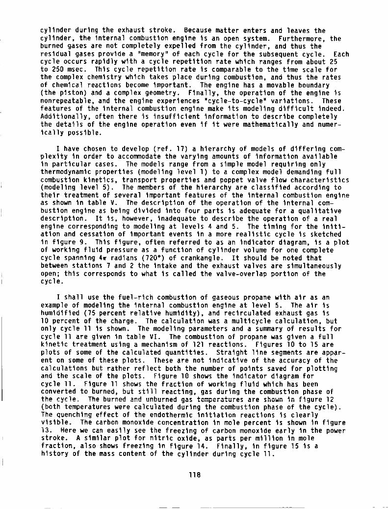
cylinder during the exhaust stroke. Because matter enters and leaves thecylinder, the Internal combustion engine Is an open system. Furthermore, theburned gases are not completely expelled from the cylinder, and thus theresidual gases provide a "memory" of each cycle for the subsequent cycle. Eachcycle occurs rapidly with a cycle repetition rate which ranges from about 25to 250 msec. Thts cycle repetition rate Is comparable to the time scale forthe complex chemistry whlch takes place during combustion, and thus the ratesof chemlcal reactions become Important. The englne has a movable boundary(the piston) and a complex geometry. Ftnally, the operation of the engine Isnonrepeatable, and the engine experlences "cycle-to-cycle" vartatlons. Thesefeatures of the Internal combustion engine make Its modeltng difficult Indeed.Additionally, often there ts Insufficient Information to descrtbe completelythe details of the engine operation even If It were mathematlcally and numer-Ically possible.
I have chosen to develop (ref. 17) a hierarchy of models of differing com-plexity In order to accommodate the varying amounts of Information availableIn particular cases. The models range from a simple model requiring onlythermodynamic properties (modeling level 1) to a complex model demanding fullcombustion kinetics, transport properties and poppet valve flow characteristics(modeling level 5). The members of the hierarchy are classified according totheir treatment of several Important features of the Internal combustion engineas shown In table V. The description of the operation of the Internal com-bustlon englne as betng divided Into four parts Is adequate for a qualltatlvedescription. It Is, however, Inadequate to descrlbe the operation of a realengine correspond%ng to modeling at levels 4 and 5. The timing for the Initi-ation and cessation of Important events In a more realistic cycle Is sketchedIn ftgure 9. This figure, often referred to as an Indicator dlagram, Is a plotof working flutd pressure as a function of cylinder volume for one completecycle spanning 4e radlans (720 ° ) of crankangle. It should be noted thatbetween stations 7 and 2 the tntake and the exhaust valves are simultaneouslyopen; this corresponds to what Is called the valve-overlap portion of thecycle.
I shall use the fuel-rich combustlon of gaseous propane with atr as anexample of modeling the Internal combustion engtne at level 5. The air Ishumidified (75 percent relatlve humidity), and reclrculated exhaust gas ls10 percent of the charge. The calculation was a mult%cycle calculation, butonly cycle 11 Is shown. The modeling parameters and a summary of results forcycle 11 are given In table VI. The combustion of propane was glven a fullklnetlc treatment using a mechanism of 121 reactlons. Figures 10 to 15 areplots of some of the calculated quantities. Straight line segments are appar-ent on some of these plots. These are not Indicative of the accuracy of thecalculations but rather reflect both the number of points saved for plottingand the scale of the plots. Figure 10 shows the lndlcator diagram forcycle 11. Figure 11 shows the fractton of working fluid which has beenconverted to burned, but still reactlng, gas during the combustion phase of................................ _ _,,,V_,o_u,_a a,_ _,,uw,, ,,, gure 12
(both temperatures were calculated during the combustion phase of the cycle).The quenching effect of the endothermtc lnltlatlon reactions ts clearlyvisible. The carbon monoxide concentration In mole percent Is shown In figure13. Here we can easily see the freezing of carbon monoxide early in the powerstroke. A stmllar plot for nitric oxide, as parts per mtlllon In molefraction, also shows freeztng In figure 14. Ftnally, tn figure 15 ts ahistory of the mass content of the cyltnder during cycle 11.
I18

REFERENCES
I. Zeleznlk, Frank J.: Thermodynamics 3. Math. Phys., vol. 17, no. 8,
Aug. 1976, pp. 1579-1610.
2. Zeleznlk, Frank 3.: Thermodynamics. II. The Extended Thermodynamic
System. J. Math. Phys., vol. 22, no. l, Jan. 1981, pp 161-178.
3. Bauer, S.H.; and Zhang, L.M.: Shock-lube Pyrolysis of PolycycllcAromatlcs-Detectlon of Soot Precursors. Shock Tubes and Waves.
Proceedings of the 14th International Symposium on Shock Tubes and Shock
Waves. R.D. Archer, and B.E. Milton, eds., Sydney Shock Tube Symposium
Publishers, Sydney, Australia, 1983, pp. 654.661.
4. Forgeteg, S.; and Berces, T.: Estimation of Entropy and Heat of Formation
of Free Radicals. I. Statistical Thermodynamic Calculation of Entropies.Acta Chlm. Acad. Scl. Hung., vol. 51, no. 2, 1967, pp. 205-215.
5. Burcat, Alexander; Zeleznik, Frank J.; and McBride, Bonnie J.: Ideal Gas
Thermodynamic Properties for the Phenyl, Phenoxy and o-Blphenyl Radicals.
NASA TM-83800, 1985.
6. Benson, S.W.: Thermochemlcal Kinetics. Second ed., Wiley, 1976.
7. Colussl, A.3.; Zabel, F; and Benson, S.W.: The Very Low-Pressure Pyrolysis
of Phenyl Ethyl Ether, Phenyl Allyl Ether, and Benzyl Methyl Ether and the
Enthalpy of Formation of the Phenoxy Radical. Int. 3. Chem. Kinet.,
vol. 9, no. 2, 1977, pp. 161-I77.
8. Zeleznlk, Frank J.: A Class of Nonldeal Solutions. I-Definltion and
Properties. NASA 1P-1929, 1983.
9. Zeleznlk, Frank J.; and Donovan, Leo F.: A Class of Nonldeal Solutions.
IT- Application to Experimental Data. NASA TP-1930, 1983.
I0. Gordon, Sanford; McBride, Bonnie J.; and Zeleznlk, Frank 3.: Computer
Program for Calculation of Complex Chemical Equilibrium Compositions and
Applications. Supplement I-Transport Properties. NASA TM-86885, 1984.
II. Gordon, Sanford; and McBride, Bonnie J.: Computer program for Calculation
of Complex Chemical Equilibrium Compositions, Rocket Performance, Incident
and Reflected Shocks, and Chapman-Jouguet Detonations. NASA SP-273, 1976.
12. Svehla, Roger A.; and McBride, Bonnie J.: Fortran IV Computer Program for
Calculation of Thermodynamic and lransport Properties of Complex Chemical
Systems. NASA TN D-7056, 1973.
13. Zeleznik, F.3.; and Gordon, S.: Calculation of Complex Chemical
Equilibria. Ind. Eng. Chem., vol. 60, no. 6, June 1968, pp. 27-57.
14. Gordon, Sanford; and Zeleznlk, Frank J.: A General IBM 704 or 7090
Computer Program for Computation of Chemical Equilibrium Compositions,Rocket Performance, and Chapman-Jouguet Detonations. Supplement l -
Assigned Area-Ratlo Performance. NASA TN D-1737, 1963.
IT9

15.
16.
17.
Zeleznlk, Frank 3.; and Gordon, Sanford: A General IBM 704 or 7090Computer Program for Computatlon of Chemlcal Equilibrium Compositions,Rocket Performance, and Chapman-3ouguet Detonations. NASA TN 0-1454,1962.
Gordon, Sanford; Zeleznlk, Frank 3.; and Huff, Vearl N.: A General Methodfor Automatlc Computatlon of Equ111brlum Composltlons and TheoretlcalRocket Performance of Propellants. NASA TN D-132, 1959.
Zeleznlk, Frank J.; and McBride, Bonnie 3.: Modeling the InternalCombustlon Engine. NASA RP-1094, 1985.
TABLE I. - COMPARISON OF PROPERTIES FOR
PHENYL RADICAL a
Property Estimated Estimatedfrom benzene from phenol
sO 300
C_ 300
C_ 500
C_ 1000
C_ 3000
Benson(ref. 6)
69.4 69.03
18.8 18.96
.... 31.03
.... 46.59
.... 59.04
69.30
19.51
31.70
46.93
59.09
aAII valuesas eu (callg-mol K).C0-85-11235
TABLE II. - COMPARISON OF PROPERTIES
FOR PHENOXY RADICAL a
Property
S° 3OO
C_ 300
C_ 500
C._6IX)
C_ 800
C_ 1000
Benson
(ref. 6)
73.7
22.5
29.8
35.8
40.6
47.5
52.3
From phenol
73.70
22.64
29.82
35.80
40.57
47.48
52. 17
aAII values as eu (cal/g-mol K). CD-8.5-17Z36
120

ORIGINAL PAGE IS
OF POOR QUALITY
CASE NO. 6668
CHEMICAL FORMULAFUEL H 2.00000OXIDANT 0 2.00000
O/F = 7.9370
THERMODYNAMIC PROPERTIES
P, MPAT, DEG KRHO, KG/CU MH, KJ/KGU,'KJ/KGG, KJ/KGS, KJ/(KG)(K)
H, MOL NT(DLV/DLP)T(DLV/DLT)PCP, KJ/(KG)(K)GAMMA (S)SON VEL,M/SEC
IABI.E Ill.THERMODYNAMIC EQUILIBRIUM PROPERTIES AT ASSIGNED
TEMPERATURE AND PRESSURE
PERCENT FUEL = 11.1894
NT FRACTION ENERGY STATE TEMP(SEE NOTE) KJIKG-MOL DEG K
1.000000 -9012.332 L 20.271.000000 -12978.762 L 90.18
EQUIVALENCE RATIO = 1.0000 PHI = l.O00O
0.10132 0.10132 0.10132 0.10132 0.10132 0.10132 0.10132 0.10132 0.10132 0.10132 0.101325500.0 5000.0 4500,0 4000.0 3500,0 3000.0 2500.0 2000.0 1500.0 1000.0 500.0
1.3416-2 1.4967-2 1.7468-2 2.3376-2 3.8936-2 6.2488-2 8.5005-2 1.0938-1 1.4635-1 2.1955-1 q.3909-155513.9 52669.0 47251.0 33833.1 12360.5 -1457.79 -6953.36 -9278.31 -10745.6 -11979.6 -13038.547961.3 45899.1 41450.5 29498.5 9758.19 -3079.30 -8145.34 -10204.6 -11438.0 -12441.1 -13269.2
-123677.1-107511.2 -91736.2 -76960.8 -64513.3 -54702.2 -46385.9 -38774.8 -31609.1 -24892.6 -18767.832.5802 32.0360 30.8861 27.6985 21.9640 17.7481 15.7730 14.7483 13.9090 12.9130 11.4586
6.055 6.141 6.450 7.672 11.182 15.383 17.438 17.951 18.013 18.015 18.015-1.00811 -1.02147 -1.06320 -1.15917 -1.16898 -1.06245 -1.01196 -1.00121 -1.00004 -1.00000 -1.00000
1.0831 1.2419 1.7935 3.2778 3.8474 2.2710 1.2997 1.0382 1.0015 1.0000 1.00004.6981 7.2046 16.3371 38.8059 39.0979 17.2068 6.6083 3.3997 2.6424 2.2907 1.95481.5032 1.3668 1.2355 1.1639 1.1268 1.1106 1.1235 1.1705 1.2124 1.2523 1.30913369.4 3041.9 2677.0 2246.2 1712.4 1341.9 1157.2 1041.3 916.2 760.2 549.6
TRANSPORT PROPERTIES (GASES ONLY)CONDUCTIVITY IN UNITS OF MILLIWATTSI(CM)(K)
VISC,MILLIPOISE 1.3674 1.2723 1.1761 1.0869 1.0207 0.94586 0.83841 0.70639 0.55364 0.37747 0.17324
NITH EQUILIBRIUM REACTIONS
CP, KJ/(KG)(K) 4.6844 7.2044 16.3359 38.8069 39.1072 17.2071 6.6077 3.3935 2.6423 2.2907 1.9548CONDUCTIVITY 12.6667 16.4726 31.4208 70.9281 79.3619 34.1601 9.6648 3.2468 1.7354 0.9740 0.3603PRANDTL HUMBER 0.5057 0.5564 0.6115 0.5947 0.5030 0.4764 0.5752 0.7383 0.8430 0.8878 0.9398
NITH FROZEN REACTIONS
CP, KJ/(KO)(K) 3.5289 3.5100 3.4743 3.3857 3.2373 3.1124 2.9951 2.8393 2.6140 2.2907 1.9548CONDUCTIVITY i0.3699 9.6043 8.7109 7.4819 5.8067 4.3630 3.3449 2.4942 1.7049 0.9740 0.3603PRANDTL NUMBER 0.4653 0.4650 0.4691 0.4918 0.5691 0.6747 0.7507 0.8041 0.8488 0.8878 0.9398
MOLE FRACTIONS
H 0.66077 0.65095 0.61751 0.50212 0.25268 0.05763 0.00517 0.00012 0.00000 0.00000 0.00000H02 0.00000 0.00000 0.00000 0.00003 0.00008 0.00005 0.00001 0.00000 0.00000 0.00000 0.00000H2 0.00387 0.01037 0.03230 0.10047 0.18534 0.13479 0.04283 0.00581 0.00020 0.00000 0.00000H20 0.00002 0.00018 0.00213 0.02961 0.23353 0.64341 0.91089 0.98950 0.99968 1.00000 1.000000 0.33098 0.32663 0.31048 0.24985 0.11877 0.02421 0.00182 0.00003 0.00000 0.00000 0.00000OH 0.00363 0.00967 0.02972 0.08948 0.15096 0.09367 0.02331 0.00214 0.00004 0.00000 0.0000002 0.00073 0.00219 0.00786 0.02845 0.05865 0.04624 0.01596 0.00238 0.00009 0.00000 0.00000
ADDITIONAL PRODUCTS NHICH HERE CONSIDERED BUT NHOSE MOLE FRACTIONS HERE LESS THAN 0.50000E-05 FOR ALL ASSIGHED COHDITIOHS
H202 03 H20(S) H20(L) CD-85-]7_6
121

ORIGINAL PAGE 15OF POOR QUALITY
TABLE IV.
SHOCK NAVE PARAMETERS ASSUMING
EQUILIBRIUm COMPOSITION FOR INCIDENT SHOCKED CONDITIONS
CASE NO. 1207
CHEMICAL FORMULA
FUEL H 2.00000
FUEL 0 2.00000FUEL AR 1.00000
O/F = 0.0000 PERCENT FUEL = 100.0000
INITIAL GAS (1)
MACH NO. 3.3528 3.5052 3.6576 3.8100
U1, M/SEC 1100.00 1150.00 1200.00 1250.00P, ATM 0.01316 0.02632 0.02632 0.02632
T, DEC K 300.0 300.0 300.0 300.0
RHO, G/CC 2.0126-5 4.0252-S 4.0252-5 4.0252-S
H, CAL/G 0.25457 0.25457 0.25457 0.25457
U, CAL/G -15.578 -15.578 -1S.578 -15.578
G, CAL/G -371.94 -360.97 -360.97 -360.97S, CAL/(G)(K) 1.2407 1.2041 1.2041 1.2041
M, MOL NT 37.654 37.654 37.654 37.654
CP, CAL/(G)(K) 0.1372 0.1372 0.1372 0.1372GAMMA (S) 1.6249 1.6249 1.6249 1.6249
SOH VEL,M/SEC 328.1 328.1 328.1 328.1
MOLES ENERGY STATE TEMPCAL/MOL DEGK
0.050000 13.324 G 300.00
0.050000 12.952 O 300.00
0.900000 9.191 G 300.00
EQUIVALENCE RATIO = 0.5000 PHI = 0.0000
3.9624 4.1148 4.2672 4.4196 4.S720 4.72441300.00 1350.00 1400.00 1450.00 1500.00 1550.00
0.02632 0.02632 0.02632 0.02632 0.02632 0.02632
300.0 300.0 300.0 300.0 300.0 300.0
4.0252-5 4.0252-5 4.0252-5 4.0252-5 4.0252-5 4.0252-S
0.25457 0.25457 0.25457 0.25457 0.25457 0.25457
-15.578 -15.578 -15.578 -15.578 -15.578 -15.S78-360.97 -360.97 -360.97 -360.97 -360.97 -360.97
1.2041 1.2041 1.2041 1.2041 1,2041 1.2041
37.654 37.654 37.654 37.654 37.654 37.654
0.1372 0.1372 0.1372 0.1372 0.1372 0.1372
1.6249 1.6249 1.6249 1.6249 1.6249 1.6249
328.1 328.1 328.1 328.1 328.1 328.1
SHOCKED GAS (2)--INCIDENT--EQUILIBRIUM
U2, M/SEC 666.94 602.16 576.32 560.44
P, ATM 0.10778 0.27659 0.32363 0.36873
T, DEC K 1528.1 1693.3 1817.1 1932.4
RHO, G/CC 3.3195-5 7.6873-S 8.3812-5 8.9778-S
H, CAL/G 91.697 114.97 132.65 149.4SU, CAL/G 13.067 27.830 39.138 49.982
G, CAL/G -1940.61 -2079.42 -222S.77 -2363.02
S, CAL/(G)(K) 1.3300 1.2959 1.2979 1.3002
M, MOL WT 38.619 38.617 38.614 38.608(DLV/DLP)T -I.00001 -1.00002 -1.00005 -1.00011
(DLV/DLT)P 1.0003 1.0008 1.0019 1.0038
CP, CAL/(G)(K) 0.1403 0.1420 0.1443 0.1478
GAMMA (S) 1.5795 1.S700 1.5576 1.5403
SON VEL,M/SEC 720.9 756.6 780.6 800.6
TRANSPORT PROPERTIES (GASES ONLY)
CONDUCTIVITY IN UNITS OF
VISC,MILLIPOISE 0.72845 0.77927
WITH EQUILIBRIUm REACTIONS
MILLICALORIES/(CM)(K)(SEC)
0.81611 0.84959
549.22 540.3S 532.52 524.96 517.29 509.40
0.41405 0.46053 0.50878 0.55917 0.61191 0.66707
2044.1 2153.0 2258.8 2360.3 2456.7 2547.39.5277-S 1.0057-4 1.0582-4 1.1118-4 1.1672-4 1.2248-4
166.17 183.16 200.60 218.59 237.18 256.35
60.929 72.259 84.16S 96.788 110.22 124.45
-2496.51 -2627.06 -2753.88 -2875.57 -2990.89 -3098.89
1.3026 1.3052 1.3080 1.3109 1.3140 1.3172
38.597 38.579 38.551 38.S10 38.452 38.378
-1.00021 -1.00041 -1.00073 -1.00123 -1.00193 -1.00286
1.0070 1.0125 1.0209 1.0330 1.0492 1.069S
0.1532 0.1613 0.1728 0.1883 0.2078 0.2308
1.5165 1.4859 1.4497 1.4110 1.3734 1.3400
817.2 830.3 840.4 848.0 854.1 859.9
0.88129 0.91160 0.94048 0.96775 0.99326 1.0169
CP, CAL/(G)(K) 0.1396 0.1415 0.1431 0.1478 0.1522 0.1613 0.1728 0.1882 0.2078 0.2308
CONDUCTIVITY 0.1536 0.1678 0.1786 0.1992 0.2158 0.2576 0.3087 0.3799 0.4721 0.5823
PRANDTL NUMBER 0.6619 0.6573 0.6539 0.6304 0.621S 0.5706 0.5264 0.4796 0.4371 0.4031
WITH FROZEN REACTIONS
CP, CAL/(G)(K) 0.1396 0.1401 0.1405 0.1408 0.1411 0.1413 0.1416 0.1418 0.1420 0.1422
CONDUCTIVITY 0.1536 0.1658 0.1747 0.1829 0.1907 0.1984 0.2058 0.2131 0.2201 0.2270
PRAHDTL HUMBER 0.6619 0.6587 0.6563 0.6540 0.6519 0.6495 0.6469 0.6440 0.6406 0.6368
P2/P1 8.191 10.511 12.298 14.012 15.734 17.500 29.334 21.248 23.253 25.349
T2/T1 S.09 _ 5.644 6.057 6.441 6.814 7.177 7.529 7.868 8.189 8.491
MZ/M1 1.0256 1.0256 1.0255 1.0253 1.0250 1.0246 1.0238 1.0227 1.0212 1.0192RHO2/RHO1 1.6493 1.9098 2.0822 2.2304 2.3670 2.4984 2.6290 2.7621 2.8997 3.0428
V2(U1-U2)M/SEC 433.06 547.84 623.68 689.56 75b.78 809.65 867.48 925.04 982.71 1040.60
MOLE FRACTIONS
AR
H
H02
H2H20
H202
0
OH
02
9.2306-1 9.2302-1 9.2294-1 9.2279-1 9.2254-1 9.2211-1 9.2144-1 9.204S-1 9.1909-1 9.1732-1
1.2073-7 8.7884-7 4.2747-6 1.5554-5 4.7175-5 1.2409-4 2.8829-4 5.9812-4 1.1195-3 1.9103-3
4,6101-8 1.5001-7 2.8252-7 4.7303-7 7.3544-7 1.0786-6 1.5029-6 1.9983-6 2.5453-6 3.1190-6
2.6458-6 1.1305-5 3.S151-5 8.8613-5 1.9569-4 3.8922-4 7.0587-4 1.1754-3 1.8088-3 2.S906-3
5.1241-2 5.1163-2 S.1019-2 5.0770-2 5".0361-2 4.972S-2 4.8791-2 4.7502-2 4.5833-2 4.3804-2
6.699-10 2.448 -9 4.449 -9 7.237 -9 1.097 -8 1.574 -8 2.147 -8 2.796 -8 3.485 -8 4.173 -8
2.8572-6 1.2578-S 3.9852-5 1.0208-4 2.2885-4 4.6242-4 8.5400-4 1.4542-3 2.3021-3 3.4157-37.5326-5 2.0713-4 4.3641-4 8.0004-4 1.3432-3 2.1036-3 3.0994-3 4.3177-3 5.7144-3 7.2211-3
2.S622-2 2.5587-2 2.5527-2 2.5430-2 2.5285-2 2.5082-2 2.4818-2 2.4497-2 2.4133-2 2.3738-2
ADDIIIONAL PRUDUCI5 wHICH wERE CON$iDkKEU bu! WHUSb MULE FRACTION5 HERE LESS THAN O.SOOOOE-08 FOR ALL
ASSIGNED CONDITIONS
03 H20(S) H20(L)
CD-85-]7225
122
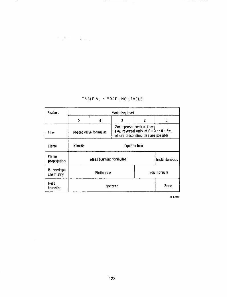
TABLE V. - MODELING LEVELS
Feature Modelinglevel
Flow
Flame
Flamepropagation
Burned-gaschemistry
Heattransfer
5 4
Poppetvalveformulas
3 2 l
Zero-pressure-drop flow;flow reversal only at O=0 or 0 =37r,where discontinuities are possible
Kinetic Equilibrium
Massburning formulas
Finite rate
Nonzero
Instantaneous
Equilibrium
Zero
CD-85-17232
123

ORIGINAL PAGE IS
OF POOR QUALITY
TABLE VI.
BORE = 10.922 CMTOTAL VOLUME = 1067.83 CC DISPLACEMENT VOLUME = 966.13 CC
IVOPEH = 699.00 DEG IVSHUT = 265.00 BEG
HEAT TRAHSFER PARAMETERS C1 = 0.000000 C2 = 0.387200E O0
KINETIC FLAME FINITE BURNING INTERVAL = 88.7 BEG WIESE
INTERNAL COMBUSTION ENGINE MODEL ZMOTTO CYCLE 11 LEVEL 5 CASE NO. 111REF: ZELEZHIK, FRANK J.; AND MCBRIDE, BONNIE J.: MODELING THE INTERNAL COMBUSTION ENGINE. NASA RP-1094, 1985.
COMPRESSIOH RATIO = 10.5 RPM = 3500.0 EGR = 0.100 T(EGR) = 900.6 K SPARK ADVANCE = 20.00 DEGFUEL PRESSURE = 1.00000 ATM MANIFOLD PRESSURE : 0.42760 ATM EXHAUST PRESSURE = 1.00000 ATMFLOWS ARE ISEHTROPIC
STROKE : 10.312 CM ROD : 17.145 CM CHAMBER AREA =129.030 SQ CM WALL TEMP = 360.0 K
EVOPEH = 465.00 DEG EVSHUT = 45.00 DEG
C3 = 0.000000 A = 0.4000 S : 0.8000
COMBUSTIOH TAU =0.8930E-04 5EC BETA = S.200
WT FRACTION EHERGY STATE TEMP
CHEMICAL FORMULA CAL/MOL DEG KFUEL C 3.00000 H 8.00000 1.000000 -24821.770 G 298.15AIR N 1.56168 0 0._1959 AR 0.00936 C 0.00032 _1.000000 -1386.340 G 298.15
w AIR INCLUDES 0.023;8 MOLE FRACTION WATER RELATIVE HUMIDITY: 0.7500
A/F: 12.5823 PERCENT FUEL: 7.3625 EQUIVALEHCE RATIO= 1.2500 PHI = 1.2647
PERFORMANCE PARAMETERS FOR ONE CYLINDER
MEAN INLET MASS FLOW RATE (G/SEC) MEAN EXHAUST MASS FLOW RATE (G/SEC)MASS PER CYCLE (G)
TOTAL 0.49685 CHARGE 12.6027FUEL 0.02860 FUEL 0.8351AIR 0.35987 AIR 10.5073
NET 12.6376
ENERGY PER CYCLE (JOULES) AVERAGE ENERGY RATE - POWER (KW)
INDICATED WORK 604.672 INDICATED POWER 11.803INDICATED PUMP WORK -86.886 INDICATED PUMP POWER -2.534HEAT LOSS 352.020 HEAT LOSS RATE 10.267CHEM. ENERGY 1305.823 EXHAUST POWER 16.593
EXHAUST 15.2527CO 0.71753NOX 0.00013NET 13.2526
CYCLE EFFICIEHCIES
NET WORK 0.243361HEAT LOSS 0.269577EXHAUST 0.435675
MISCELLANEOUS
INDICATED MEAN EFFECTIVE PRESSURE (ATM)PUMP MEAH EFFECTIVE PRESSURE (ATM)MEAN TORQUE (NEWTON-METERS)
COMPOSITE EXHAUST GAS MOLE FRACTIONS AT 900.63 K AND 1.0000 ATMAR 0.007952 CH4 0.000914 CO 0.052088C2H4 0.000131 H2 0.026S69 H20 0.169_7602 0.000070
FRESH CHARGE MOLE FRACTIONS AT 292.50 K AND 0.4276 ATM MOLECULAR WEIGHT :AR 0.000861 CH4 0.000099 CO 0.0056_3 C02C2H_ 0.00001_ H2 0.002878 H20 0.018359 H2C3H8 0.0_3867 AIR 0.847803
NOTE: INLET AND EXHAUST VALUES CALCULATED WHEN THE VALVES CLOSE.
COMPUTER CYCLE TIME: 48.858 SEC
4.1338-0.887625.2886
MOLECULAR WEIGHT : 26.947CO2 0.077497 C2H2NO 0.000009 N2
29.1920.008395 C2H20.071827 02
0.0022390.6630_1
0.0002_30.000008
C0-85-17224
124
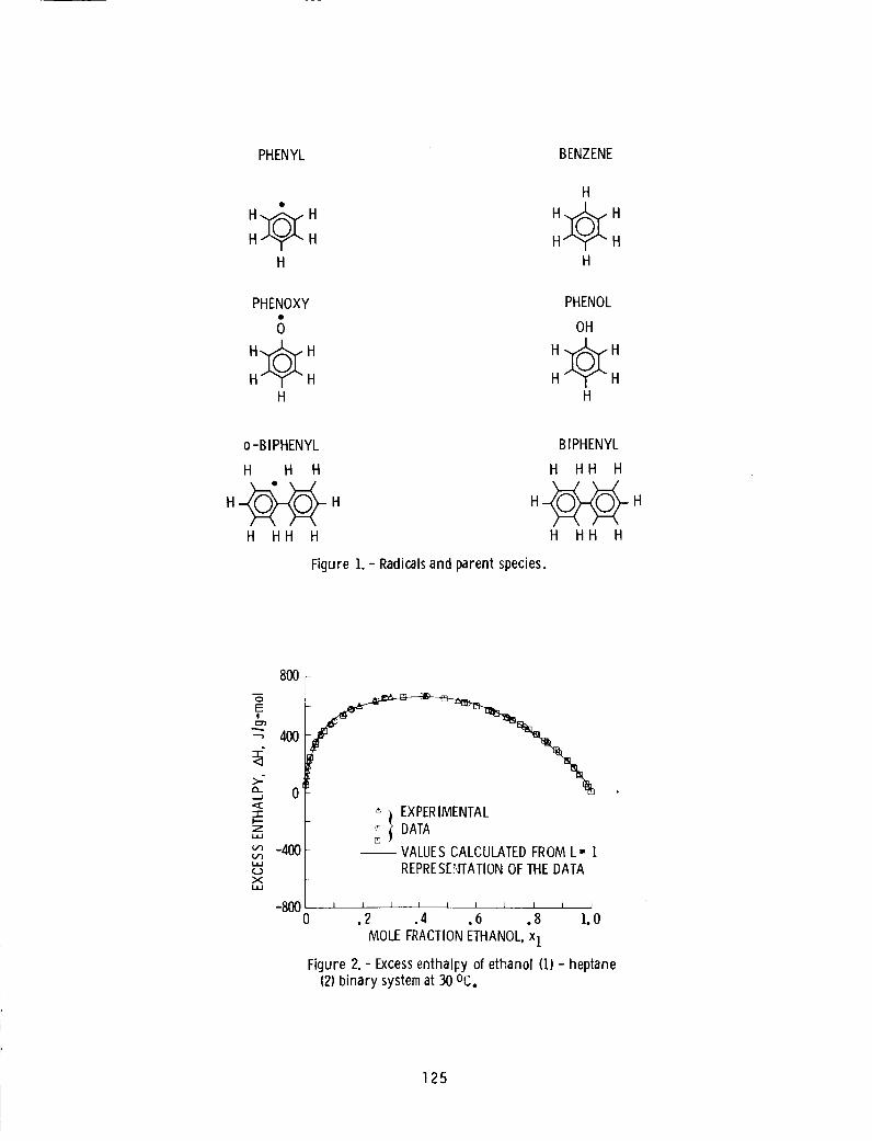
PHENYL
H H
H
BENZENE
H
HH
PHENOXY
HH
PHENOL
OH
HH
o-BIPHENYL
H H H
H HH H
BIPHENYL
H HH H
H HH H
Figure 1.-Radicalsand parent species.
0
E!
>:
:3=I.=.zI..i,.I
(./3
xILl
8OO
4OO
-4OO
-8OO0
} EXPERIMENTAL® DATA
-- VALUESCALCULATEDFROML= 1REPRESEHTATIONOFTHEDATA
I I I I I I I I I I
.2 .4 .6 .8 1.0
MOLEFRACTIONETHANOL,x1
Figure 2. - Excessenthalpy of ethanol (1) - heptane(2) binary systemat 30 OCo
125

0
E!
,....,.
"I-
ZL.iJ
l,JJ
Xl.J.J
1200
800
4O0
-4OO
-8OO0
EXPERIMENTALDATAVALUESCALCULATEDFROML" IREPRESENTATIONOF DATA
] I I I ±__ I I I I
.2 .4 .6 .8
MOLEFRACTIONETHANOL,x1
Figure 3. - Excessenthalpy of chloroform (1) -ethanol (2) binary system at 50 °C.
I
1.0
B0
E!
I.,m-,£:
o
._Jo
1.1_o
1.1.1
"l-
J
I_lJ
g
1250
1050
85O
65O
45O
250
TEMPERATURE,oC
__\ . 20
-, 25
__._J _ 1 A L i _ ] ] I
i.._ ._.u 4.J u.u 7.5MOLALITY
Figure 4. - Integral heat of solution of sodiumchloride in water.
126
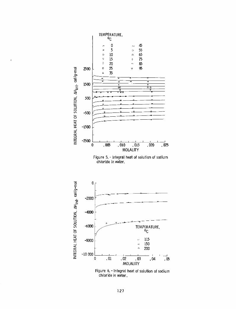
'_ 25OOE!
a. 1500r-
°_
N
_ 5O0
_ -500I.I_
oI---
w
_: -1500
r_
-2500z
TEMPERATURE,oC
_- 0"_ 5'_ 10o 15o 20D 25_, 35
q
45
55
6575
o 85
95
o o
co oo
0 0u oo ou u u
°
n ,7
17 r/
©
0 0 -
n o
I I l I I I I I I I
0 .005 .010 .015 .020 .025
MOLALITY
Figure 5.- Integral heat of solutionof sodiumchloride in water.
0
E!
e-o_
o
:D
0
I--
1.1_1-I'-
ILl
Z
0
-2_0
-4_0
_0
-8_0
-10000
TEMPERATURE,oC
115150200
I I I I I I I I I I
• 01 .02 .03 .04 .05MOLALITY
Figure 6. - Integral heat of solutionof sodiumchloride in water.
127

0
0E -0.3I
3_, -0.6
_ -0.9
_ -1. 2
.-r-
"I.50
TEMPERATURE,Oc
,:; 2580
100,_ 120o 140
_ 0 160o180
. O0
I i I J I i l I I
.5 1.0 1.5 2.0 2.5MOLALITY
Figure l.- Excessheat capacity of aqueoussodiumchloride solutions.
128
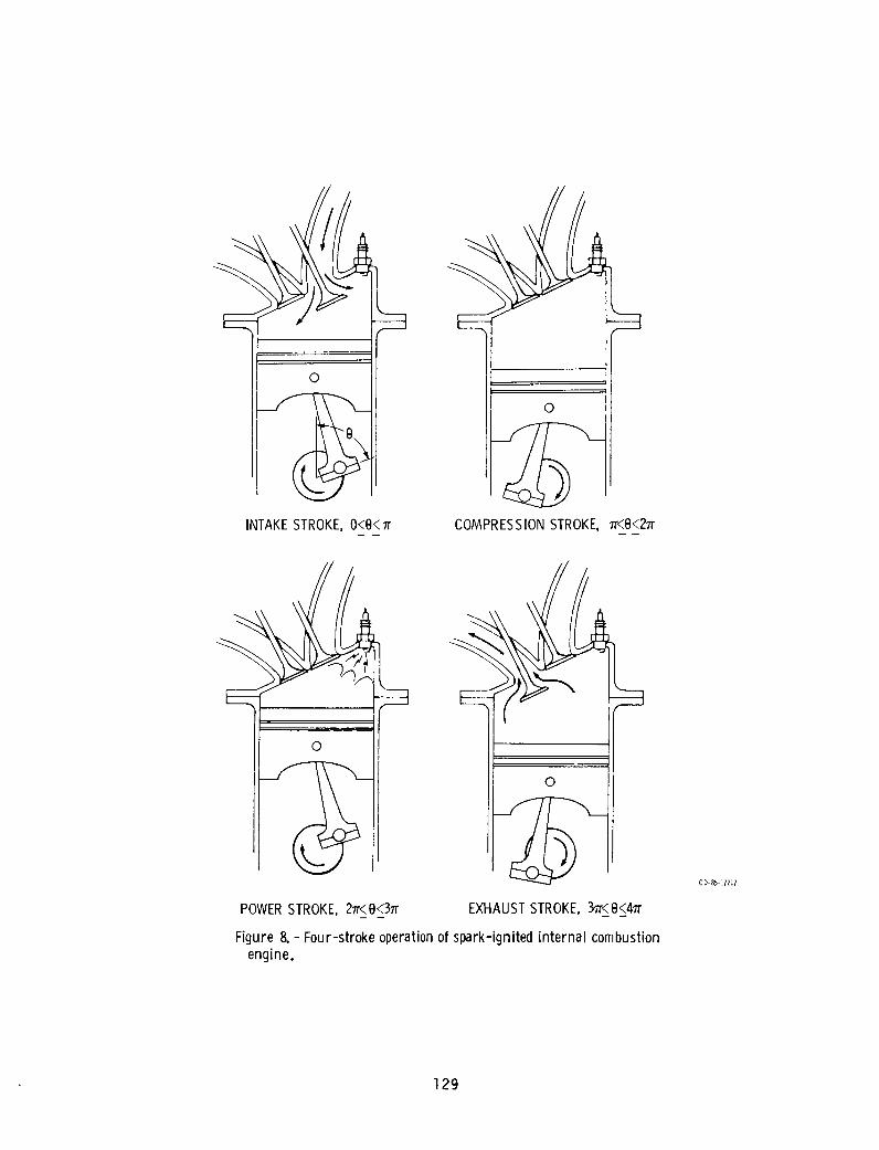
0
INTAKESTROKE,0<8<_
IIoCOMPRESSIONSTROKE, 7r<O<27r
0
0
POWERSTROKE,27r<8<37r EXHAUSTSTROKE,37r<e<47r
Figure 8. - Four-stroke operation of spark-ignited internal combustionengine.
CD-85-I/217
129
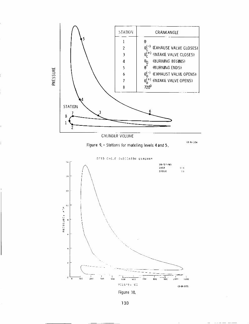
"--I
r'_
STATION CRANKANGLE
0
O(c-) (EXHAUSEVALVECLOSES)
O_+) (INTAKEVALVECLOSES)
4 00 (BURNINGBEGINS)\ 5 8''_ (BURNINGENDS)
X 6 O{o-) (EXHAUSTVALVEOPENS)
\ X 7 0(o+) (INTAKEVALVEOPENS)
STATION _
1 _2
CYLINDERVOLUME
Figure 9.- Stations for modeling levels 4 and 5.CD-85-I12_
I0
LJ
C_COLLJOCCL
6
q
00
OTTO CYCLE INDICATOR DIAGRAM
\\\
\\
\
I __1_ ..... l
IOO _oo 300
\\
'_oo 50o 600
VOLUMEp CC
08/2?/85
CASE 111
CYCLE 11
I I I I700 800 900 1000 1100
CD-$5-17221
Figure 10.
130

uJ
I--
odLLJQ.:IEUJ)--.
__)
>-¢..3
E3)--
ORIGINAL PAGE IS /-'"
OF. POOR
jJ
Q
_J\mo
I, I [ I J I _ I
_ N N g N _ N g
_30 =3_Nl_3dH31
Q4
oo
o
o
o
uJ
o,:o
\
131
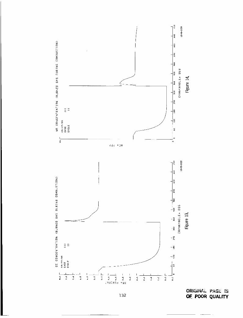
z
i.--co
=E
C9
{Z
E:]
CO
CO
0LIJZ
v
I---
C3;Z u_
uJ
o _ _
I
W
Ndd _QN
u
COuJQ
o
LLJ
# -.
QdC)
/z
cov
i-
< =zQd
- /C3
C3 (_ uj u.J..J
CJ <c >-o r3 {3
/I I I I L _SL • I I I I I I I I
iN33_3d 6Q3
A(..)
COLU
UJ ji I
CO O_z l.-
E:rlc_ z oio ,¢ u_
0_c3
132ORIGINAL PAG_ IS
OF.. POOR QUALITY
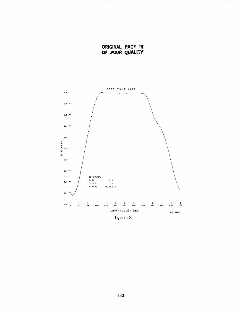
ORIGINAL PAGE 19
OF POOR QUALITY
0.9
0.8
0.7
0.6
X<[:
0,3
0°2
0.1
OTTO CYCLE MASS
0B/27/85
CASE I I I
CYCLE 11
501 G
I ] ] I J I I I 1 J I I60 Z20 IIBO 2_'0 300 360 q'20 _.$o 5_'0 600 660 720
CRANKANGLE, DEGCO-8S- lTZ18
Figure 15.
133

N87-20275
EFFECT OF FLAME-IUBE HEAD STRUCIURE ON COMBUSIION CHAMBER PERFORMANCE
Gu Minqql
Shenyang Aero-Englne Research InstituteShenyang, People's Republic of China
This paper presents the experimental combustion performance of a pre-
mixed, pilot-type flame tube wlth various head structures. The test studycovers an extensive area: efficiency of the combustion chamber, quality of
the outlet temperature field, limit of the fuel-lean blowout, ignition per-
formance at ground starting, and carbon deposition. As a result of these
tests, a nozzle was found which fits the premlxed pilot flame tube well. The
use of this nozzle optimized the performance of the combustion chamber.
lhe tested models had premlxed pilot chambers with two types of alr-film-
cooling structures, six types of venturl-tube structures, and secondary fuel
nozzles with two small spray-cone angles.
INTRODUCIION
After a period of engine operation, a premlxed pilot-type flame tube
(fig. l) with a pressurized fuel nozzle may have difficulty in starting.
Sometimes the pilot chamber may not ignite at all; this seriously affects the
starting performance of the engine. This problem is generally believed to be
due to carbon deposition in the premlxed pilot chamber (8 g carbon deposited
in a single premlxed pilot chamber after 190 min of running). In the case of
high-load running, the gas temperature in the center of the premixed pilot
chamber can be raised as high as 1200 °C; this can make the high-denslty fuel
spray crack and deposit on the downstream section of the nozzle. In addition,the wall temperature would be high, causing the fuel spray to form coke on the
wall, which (coupled with fuel deposition) would make the wall rough. Then the
carbon particles would hit the cores of deposition and would be deposited on
the wall. Thus, the wall becomes uneven and very rough. When the fuel spray
again hits the wall and flows on its uneven soft carbon layer, the fuel film
is also very uneven (unlike the film on a smooth metal wall). As a result, the
spray quality becomes very poor and the engine fails to start.
The objective of this experiment was to improve the ground starting per-
formance while not damaging the other types of combustion performance. The
study concentrated on the effect of premlxed pilot chamber structures and
nozzle spray angles on combustion performance.
This paper presents a study of the effect on combustion of (1) pre-
m_xed pilot chambers with air-film-coollng and venturl-tube structures and
(2) small-angle secondary nozzles. It emphasizes their effects on groundstarting performance and on carbon deposition within the pilot chambers.
_ESI MODELS
Premlxed Pilot Chamber With Air-Film-Cooling Structure
It is known that the alr-film-cooling structure enables free carbon
particles to be carried away by the film-coollng air flow, thus reducing or
135
..... p NOT

avoiding the contact of these particles with the wall. This helps reduce the
wail temperature. Two models were evaluated (fig: 2). Eighty film-coollng
holes (@2) were added to the wall of these two premixed pilot chambers. The
ratio of the cooling-hole opening area to the total opening area in the flame
tube wall was 0.022. The air velocity in the outlet of the alr-film-coollngring was 15 to 26 m/sec.
Premixed Pilot Chamber With Venturi-Tube Structure
A venturi tube was mounted in the rear of the swirler (fig. 3). It madethe fuel injected from the nozzle hit the venturl-tube wall and then mix wlth
the air coming from the inner section of the swirler, thus avoiding contact ofthe fuel wlth the flame tube wall. In addition, because the venturi tube was
used, the position of the reclrculation zone moved further downstream of the
nozzle; as a result, the temperature of the carbon-generatlng zone downstream
of the fuel nozzle was reduced. This helped reduce the carbon particles.
S_x venturi tubes of different sizes were evaluated. (See table I andfig. 4.) The ratio of the outer to the inner area of the swlrler was 1.16
when the venturi tube was mounted.
Secondary Nozzle With Small Spray Angle
Fuel entered from the centrifugal nozzle in the ignition process in order
to reduce or eliminate the probability of the sprayed fuel hitting the"wall.
1wo kinds of small spray-angle secondary nozzles were studied. (See table II
and fig. 5.) The spray angle was made small enough that the spray would not
hit the inner wall of the premlxed pilot chamber. Thus, the fuel spray cone
was not impaired. The fuel-alr ratio was appropriate near the ignitor, and a
good starting performance was maintained (even if there was carbon depositionin the pilot chamber).
RESUI_IS AND ANALYSIS
Amount of Carbon Deposition in Premlxed Pilot Chamber
lhe experimental results for various models are listed in table III.
(Results for the original flame tube are included for comparison.) The
results indicate that the venturi tube is the best structure for eliminating
carbon deposition. There was almost no carbon deposition in the pilot chamber,and there was only a small amount of carbon deposition in the 20- to 30-mm
position downstream of the pilot chamber exit. The objective of reducing car-bon deposition in the pilot chamber was achieved.
Results from the water analog test indicate that there was no reclrcula-
tion zone in the venturl tube. The recirculation zone in the premlxed pilotchamber was located far downstream of the nozzle (fig. 6). The heat radiation
from the flame-tube center to the nozzle was blocked outside of the venturi
tube, thus reducing the temperature downstream of the nozzle. This had a
determinate effect on the reduction of the carbon particles. It was for
136

this reason that the amount of carbon deposition in the flame tube with a ven-furl tube was obviously reduced.
Adding an alr-film-coollng structure in the premlxed pilot chamberhelpedreduce carbon deposition. The reduction rate was usually as muchas 20 to 30percent near the alr-film exits. But, at the exits of the air films, the airvelocity was small, so was the alr-flow momentum. Nevertheless, the momentumof the fuel injected from the nozzle was rather large, so the film flow couldnot prevent the fuel droplets from hitting the wall. It is only possible forthe film air to bring away free carbon particles. For this reason, thisstructure is not very effective in reducing carbon deposition.
Ground Starting Performance
The results for five models at the ground starting ignition condition areshownin figures 7 and 8 where V2 is the inlet velocity of the combustionchamber. The curves of figure 7 indicate that there is an optimal value foreach curve. This velocity ranges from 15 to 20 m/sec. The ignition perform-ance was best for the flame tube with a model I venturl tube.
Figure 8 indicates that the ground starting ignition performance improved
greatly when model I and II nozzles were used under carbon deposition condi-
tions in the premlxed pilot chamber. At 17.5 m/sec of inlet velocity the
fuel-lean ignition limit improved; the limiting alr-fuel ratio increased from
36.8 to 63.2. It is readily seen from these results that, under the carbondeposition condition in the premlxed pilot chamber, adoption of a small-angle
secondary nozzle obviously improves the ground starting ignition performance.
In addition, it is known from the curves that when carbon is deposited in
the premlxed pilot chamber the alr-fuel ratio of the fuel-lean ignition limitdecreases from 47 to 36. This confirms that carbon deposition in the prem_xed
pilot chamber deteriorates the ground starting ignition performance.
Outlet Temperature Field of Combustion Chamber
Table IV shows the test results of various venturl-tube models. It is
readily seen from the table that the size of the venturl tube mounted in the
premlxed pilot chamber has a great effect on the combustor outlet temperaturefield. The outlet temperature distribution factor (OIDF, table IV) of the
model V combustion chamber was 0.155; this was much better than that for the
original model (0.229). lhe OIDF's of models I and II were similar to that of
the original model, but those of models IV and VI were inferior to that of the
original model.
lhe convergent angle of the front section and the outlet angle of the
venturl tube have an obvious effect on the combustor outlet temperature dis-
tribution. When the convergent angle of the front section of the venturl tube
increases, the uniformity of the combustor outlet temperature field decreases.
When the convergent angle was increased from 27o34 ' to 67o22 ', the OTDFincreased from 0.209 to 0.301. When the venturl-tube outlet angle became
rather small, excessive fuel concentrated in the center of the flame tube;
this caused the temperature to rise in the center region and the outlet
137

temperature distribution to deteriorate. For example, reducing the outlet angleof the venturt tube from 88 ° to 56 ° increased the OTDF from 0.155 to 0.301.
Adoption of a secondary nozzle with a small spray angle also improved theuniformity of the combustor outlet temperature fteld- the OTDF of model II was0.175, the radial temperature distribution factor (RTDF, table IV) was 0.077.
Stability of Combustion Chamber
Figure 9 shows experlmental results of the fuel-lean blowout llmlt forvarious models. The shapes of the curve are nearly the same for variousmodels. The fuel-lean blowout llmtt for the model II venturl tube was widerbecause this venturt tube had no throat section; thus, a small rectrculatlonzone was formed inside the venturi tube. The size of the rectrculatlon zone
was limited to the nozzle diameter range (fig. 10).
The fuel-lean blowout limits of the model III, IV, and V venturl tubes were
narrower. It Is known from water analog test results that there is a high-
speed rotating flow in the throat section of a venturl tube (fig. ll). Thlsunstable flow deteriorates the fuel-lean blowout limit.
When a secondary nozzle with a small spray angle was adopted, the fuel-
lean blowout limit improved In the wlde velocity range.
CONCLUSIONS
This study led to the following conclusions:
(I) Adoption of the secondary nozzle wlth a small spray angle not only
solves the engine's starting ignition problem when there Is carbon deposition
In the premlxed pilot chamber but also extends the ground starting ignition
range and improves the uniformity of the combustor outlet temperature field.
(2) Adoption of an alr-fllm-coollng structure reduces the amount of carbon
deposition on the wall of the premlxed pilot chamber. But since there Is only
limited cooling alr available, it Is not easy to totally eliminate the carbon
deposition In the premlxed pilot chamber.
(3) Mounting the venturl tube in the rear of the swlrler Is effective In
eliminating carbon deposition In the premlxed pilot chamber. But the geometryof the venturl tube affects the uniformity of the _ombustor outlet temperature
field and the ground starting ignition performance; therefore, characteristic
geometric parameters of the venturl tube have to be elaborately adjusted.
BIBLIOGRAPHY
Gu, M.Q.: Study of Premlxed Pilot Chamber Wlth Alr Fllm Cooling Structure.
December 13, IgBO.
Llu, Q.G.: Investigation of Carbon Deposition Performance on the Wall of a
Flame Tube. April 28, lgBO.
138

Shang, M.Z.: Effect on Igniting Performance for Different Flame Tubes andFuel Nozzles. June lO, lg82.
Yang, A.L.: Report of Water Analog on Solving the Carbon Oepos%tlon Failureof Flame Tubes. April lO, 1982.
Yang, X.Z.: Test Report of Ground Starting Ignition of a Combustion Chamber.
September 20, 1981.
TABLE I. - CHARACIERISIIC DIMENSIONS OF VENIURI TUBE
Model
|
I
II
III
IV
V
VI
Inlet
Diameter,
mm
42
Length,mm
36
2525
20
20
15
Throat
diameter,mm
Outlet
cone
angle,deg
3O
423O
3O
3O
15
56°
36o32 '
56°
56°
88°
0°
Outlet
diameter,mm
40
45.340
35
40
15
TABLE If. - CHARACTERISllCS OF NOZZLE
Model Spray Fuel
angle, flow,
_sec Gf' sec'
deg llter/hr
Fuel supply pressure,
_double,
degGfdouble,
llter/hr
P1sec
OriginalI
II
91
51
62
= lO kg/cm 2
24.6
24.6
23.16
Fuel supply pressure,
PTdoubl e = 30 kg/cm 2
602.4
602.4
593.4
103
I00
I00
139

TABLE III. EFFECI OF VARIOUS MODELS
ON CARBON DEPOSLIION
[Test conditions at inlet of combustion chamber:
air pressure, P_, 6 kg/cm2; air temperature,
T_, 595 K; air flow, Ga, 3.135 kg/sec; air-
fuel ratio, a/f, 70; test duration, 2.5 hr.]
Model
Original flame tubeModel I venturl tube
Model Vl venturl tube
Model I air film cooling
Model II air film cooling
Amount ofcarbon
deposition,g
1.3
.0720
1.076
.932
Relative
percentage
I005.54
0
82.871.7
TABIE IV. EFFECI OF VENTURI-TUBE GEOMEIRY ON PERFORMANCE OF COMBUSIION CHAMBER
[lest conditions at inlet of combustion chamber: air pressure, P_,
6 kg/cm2; air temperature, l_, 695 K; air flow, Ga, 3 kg/sec;
air-fuel ratio a/f, 52.2.]
Model Original I 1L III IV V VI
Inlet convergent angle
Outlet cone angleaOIDF
aRIDF
an C
,l
0.229
.083
.984
27034 '
56°
0.209
.143
.984
0.223.098.975
62°
56°
0.236
.133
.988
67°22 '
56°
0.301
.138
.997
67o22 '
88°
0.155
.085
.979
122 °
0.406
.llO
.929
*) • = I_)/(T_ T_); andaOIDF = (l_ - 12 /(l_ - T_), RTDF (13 - -max av max(h) av
= pfficipncv nf cnmhlJKtlnn ch_mhpr whprp I* it thp _vpr_aP cnmhiJRtlnn
c .... _ ................................. 3av ........... _..............
outlet temperature _* the maximum combustor outlet temperature, and T*' 3ma x 3max(h)
the maximum combustor outlet temperature along the blade height.
140

....iJ_' 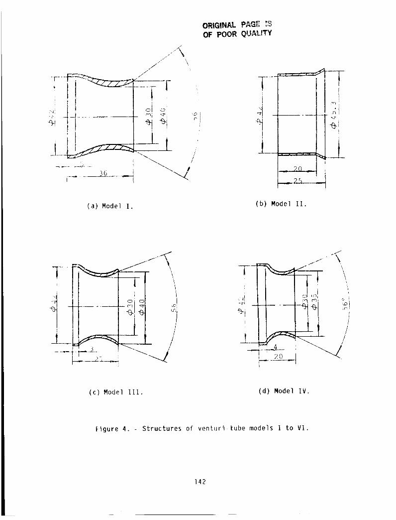
J
t
L-'L,
_ .... r_. _ ....
/
36 I
J
ORIGINAL P_.G_ _S
OF POOR QUALITY
w ---
_20:_
_25
fi
/j
_._L.
k
(a) Mode] 1. (b) Model If.
• ' i
•_ _1 '_1 ,
-5-! _1 ,_-_iti/
//
I_ 20
_ u7 i
-.-\\\
\
o i,.elLC_I
/
//
(c) Model Ill. (d) Model IV.
Figure 4. Structures of venturi-tube models I to VI.
142
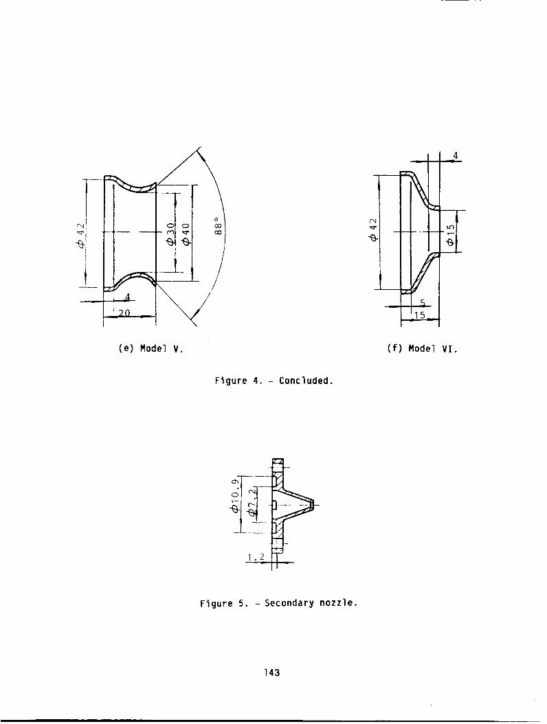
Z
!i
\
o
/
//
C_
P__ L.-...--
//
(e) Model V. (f) Model VI.
Figure 4. - Concluded.
Figure 5. - Secondary nozzle.
143

.I-_--'W ", ",.."-r'.,_i _ '_ ,,_ I
_>"\,_ " ,-. " - "i , iii _ |
Figure 6. -Flow spectrum in flame-tube head
with model I venturi tube.
a/f
6O
45
30
T
tI
..... ,--" 1.... ,----7oz ]gJna] iLLII__ , ,I
, , i _ J[ i ,
0 5 ! 0 _ _ 20 2_ 30
1 _ i i I II i : ! '
V:{ m/sec
Figure 7. - Effect of venturl-tube size on
ground ignition performance. Test condi-
tions at combustion chamber inlet: air
pressure, P_, 1.04 kg/cm2; air tempera-
ture, l_, 331K.
144
01[ poOR QUALITY
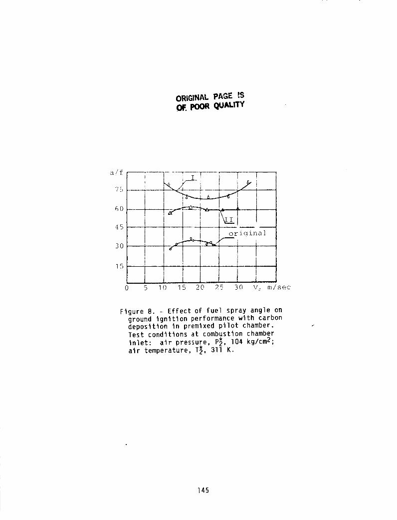
ORIGINAL PAGE: ZS.OF.POOR R_JALITY
a/f
75
60
45
30
15
_7---__ ......-T-T.,T_ ____T___._7______-a-.________ .... __._ ,._/ :
ft i lllil....0 5 10 15 20 25 30 V_ m/sec
Figure 8. -Effect of fuel spray angle on
ground ignition performance with carbondeposition in premlxed pilot chamber.Test conditions at combustion chamber
inlet: air pressure, P_, 104 kg/cm2;air temperature, T_, 311 K.
145
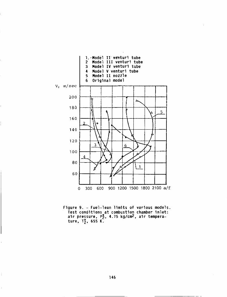
V2 m/sec
2OO
180
160
140
120
I00
80
6O
1.,Model It_venturl tube2 Model III venturl tube3 Model IV venturl tube4 Model V venturt tube5 Model II nozzle6 Original model
• t m'
II
,it
i !
0 300 600 900 1200 1500 1800 2100 a/f
Figure 9. - Fuel-lean limits of vartous models.Test conditions at combustion chamber inlet:atr pressure, P_, 4.75 kg/cm2, air tempera-ture, T_, 655 K.
146

ORIGINAL PAGE IS
OF POOR QUALITY
'..:-..:.;-- _,_,fV"_-I'_ _'. "- "-.: ". -'._ _
"__ X"_'?___ ] " " "" ! A ! , I'll
Figure I0. - Flow spectrum in flame-tube headwlth model II ventur1 tube.
Figure II. - Flow spectrum in flame-tube headwith model III venturl tube.
147

N87-20276
EXPERIMENTS AND MODELING OF DILUTION JET FLOW FIELDS
James D. Holdeman
NASA Lewis Research Center
Cleveland, Ohlo
This paper presents experimental and analytical results of the mixing ofsingle, double, and opposed rows of Jets wlth an isothermal or variable-
temperature maln stream In a straight duct. Thls study was performed to inves-tigate flow and geometric variations typical of the complex, three-dlmenslonal
flow field In the dilution zone of gas-turblne-englne combustion chambers.
The principal results, shown experimentally and analytically, were the
following: (1) variations in orifice slze and spacing can have a significanteffect on the temperature profiles; (2) similar distributions can be obtained,
independent of orifice dlameter, if momentum-flux ratio and orifice spacing arecoupled; (3) a flrst-order approximation of the mixing of jets wlth a variable-
temperature maln stream can be obtained by superimposing the maln-stream and
jets-ln-an-lsothermal-crossflow profiles; (4) the penetration of Jets issuingfrom slanted slots Is similar to that of Jets from circular holes, but the
mixing is slower and is asymmetric wlth respect to the Jet centerplanes, which
shift laterally wlth increasing downstream distance, (5) double rows of Jets
glve temperature distributions similar to those from a single row of equally
spaced, equal-area circular holes; (6) for opposed rows of Jets, wlth the ori-
fice centerllnes In llne, the optimum ratio of orifice spacing to duct heightIs one-half the optimum value for slngle-slde injection at the same momentum-flux ratio; and (7) for opposed rows of Jets, with the orifice centerllnes
staggered, the optimum ratio of orifice spacing to duct height Is twice theoptimum value for slngle-slde injection at the same momentum-flux ratio.
In illustrating these results, the mean temperature measurements are com-
pared wlth profiles calculated using an empirical model based on assumed verti-cal profile similarity and superposltlon and wlth distributions calculated
using a three-dlmenslonal elllptlc code that had a standard k-_ turbulence
model. The empirical model predictions are very good within the range of the
generating experiments, and the numerical model results, although they exhibit
too little mixing, correctly describe the effects of the principal flow andgeometric variables.
Aj/A m
C
Cd
D
SYMBOLS
Jet to maln-stream area ratio, A_/Am- = (_/4)/[(S/Ho)(Ho/D)2 ]
for one-slde injection and (_/2)/[(S/Ho)(Ho/D) 2] for two-slde
injection
(S/Ho)_-', eq. (3)
orifice discharge coefflclent
orifice diameter
149

Dj
DR
H0
J
M
R
S
SX
1
IJ
Im
U
Um
vj
÷
w5/2
wj/w I
Z
e
ec
emln
Dgq
jet to maln-stream density ratio, DR _ Tm/T j
duct height
jet to maln-stream momentum-flux ratio, J = (DR)R 2
jet to maln-stream mass-flux ratio, M = (DR)R
jet to maln-stream velocity ratio, R = Vj/U m
spacing between orifice centers
spacing between orifice rows
temperature
jet exit temperature
maln-stream temperature
velocity
maln-stream velocity
jet velocity
jet half-wldths above (÷) or below (-) the centerllne (ref. 5)
jet to tqtal mass-flow ratio, wj = DR (Cd)
(_J (Cd(Aj/Am)/(1 ÷ )(Aj/Am_ /WT _/_ )J
downstream coordinate (x = 0 at injection plane)
cross-stream (radial) coordinate (y = 0 at wall; y = Yc at location
of mln_mum temperature in a llne x = constant and z = constant)
lateral (circumferential) coordinate (z = 0 at centerplane)
(Tm - T)/(T m - Tj), eq. (1)
temperature difference ratio at Yc
minimum temperature difference ratio above (÷) or below (-) the
centerllne, (fig. 4)
INTRODUCIION
The problem of jets in crossflow has been rather extensively treated in
the literature, to the point that it can almost be called a classical three-
dimensional flow problem. Although these studies have all contributed to the
understanding of the general problem, the information obtained in any given
150

ORIGINAL PAGE IS
OF POOR QUALITY
study is naturally determined by the motivating application and therefore maynot satisfy the specific needs of diverse applications.
Consideration of dilution zone mixing in gas-turbine combustion chambers
has motivated several previous studies of the mixing characteristics of Jets
injected normally into a ducted crossflow (refs. l to 12). One factor makingthe combustor dilution zone jet-ln-crossflow application unique is that it is
a confined mixing problem - lO to 50 percent of the total flow enters through
the dilution jets. The result is that the equilibrium temperature of the exit-
ing flow may differ significantly from that of the entering maln-stream flow.
lo control or tailor the combustor exit temperature pattern, we must be able
to characterize the exit distribution in terms of the upstream flow and geo-metric variables, lhls requires that the entire flow field be either known ormodeled.
Empirical correlation of experimental data can provide an excellent pre-
dictive capability within the parameter range of the generating experiments
(e.g., refs. 4 to 6), but empirical models must be used with caution, or not
at all, outside this range. Physical modeling, in various levels of sophisti-
cation and complexity, may be used to obviate this weakness. In this regard,
several one- and two-dimenslonal, integral and differential Jet-ln-crossflow
models have been developed and shown to give, for example, trajectory predic-
tions that are in good agreement with experiments, lhese models may provide
insight into the dominant physical mechanism(s) and may predict some of the
characteristic parameters well, but they rarely provide sufficient information
to quantify the flow field in three coordinate directions.
Recently, rapid advances have been made in the capability of computational
fluid dynamics models and in their application to complex flows such as jetsin crossflow (refs. 13 to 16). These models are, however, still in the devel-
opment and verification stage. They have been shown to be capable of predict-
ing trends in complex flows, but their capability to provide accurate,
quantltive, and grld-lndependent calculations of these flows has not yet been
demonstrated (refs. 14 to 16).
PREVIOUS RESULTS AND THE CURRENT STUDY
lhe study in references 17 to 19 was performed to extend the available
experimental data on, and the empirical correlations of, the thermal mixing of
multiple jets in crossflows so that they would include geometric and flow
variations characteristic of gas turbine combustion chambers - namely, variable
temperature main stream, flow area convergence, nonclrcular orifices, and
double and opposed rows of jets. These experiments are a direct extension of
those in reference I. The effect on the dimensionless temperature distribu-
tions of varying the jet to maln-stream density ratio, the momentum-flux ratio,and the orifice size and spacing are presented in reference 2.
From the data in reference I, an empirical model was developed (refs. 4and 5) for predicting the temperature field downstream of a row of jets mixing
with a confined crossflow. The effects of separately varying the independentflow and geometric variables and the relations among these variables which
optimize the mixing are reviewed in reference 12. lhis study was conducted
using an interactive microcomputer program that is based on the empirical model
of reference 5.... ..,
151
The results of these investigations may be summarizedas follows: (I)
m_xlng improves with increasing downstream distance; (2) the momentum-flux
ratio is the most significant flow variable; (3) the effect of density ratio
is small at constant momentum flux ratio; (4) at any given momentum-flux
ratio, decreasing orifice spacing while maintaining a constant orifice diameter
reduces penetration and increases lateral uniformity; (5) increasing orifice
diameter while maintaining a constant spaclng-to-dlameter ratio improves pene-tration but increases lateral nonunlformlty; (6) increasing orifice diameter
at a constant orifice spacing increases the magnitude of the temperature dif-
ference, but jet penetration and profile shape remain similar; (7) profiles forconditions with equivalent coupling of orifice spacing and momentumflux ratio
show similar distributions; and (8) smaller momentum-flux ratios (larger spac-
ing) require a greater downstream distance for equivalent mixing.
Results from the experiments in references 17 to 19 that are considered
in this paper include the effects of variations in orifice size and spacing,
coupled spacing and momentum-flux ratio, variable temperature main stream,noncircular orifices, and double and opposed rows of Inllne and staggered jets.
Also, temperature field measurements from several experiments are compared with
distributions calculated using an empirical model based on assumed vertical
profile similarity and superposltlon (refs. 17 to 19) and using a three-
dimensional elliptic code with a standard k-_ turbulence model (ref. 14). Theresults show the capability of these models to predict the effects of the
principal flow and geometric variables.
A more complete presentation of the experimental results and a discussion
of the empirical modeling performed in this study are given in references l,
4, and ll to 19. Selected experimental and analytical results from these
studies and from reference 14 are also given in references 2, 5, and 20 to 23.
FLOW FIFI_D DESCRIPIION
Figure l shows a schematic of the dilution Jet flow field for jet injec-
tion from the top wall. The temperature field results are presented in three-
dimensional oblique views of the temperature difference ratio e:
T - lm
e-1 -T (1)m j
A sequence of experimental profiles of this parameter at several Ioca-
tions downstream of the injection plane is shown in figure 2. In the three-
dimensional plots the temperature distribution is shown in the y,z-planesnormal to the main flow direction x. The coordinates y and z are, respec-
tively, normal and parallel to the orifice row. Note that the Jet fluid is
identified by the larger values of the e parameter (i.e., e = 1 if T = lj,and e = 0 if l = Tm). lhe equilibrium e for any configuration is equal
to the fraction of the total flow entering through the dilution jets wj/w l.
lhe orifice configurations investigated are shown in figure 3. The pri-
mary independent geometric variables for each orifice configuration are the
spacing between adjacent orifices S, the orifice diameter D (for nonclrcularorifices, th_s is taken as the diameter of a circle of equal area), and, for
double rows, the axial spacing between rows Sx. lhese are expressed in
152

dimensionless form as the ratio of the orifice spacing to duct height S/Ho,the ratio of the duct height to orifice diameter Ho/D, and the ratio of theaxial spacing to the duct height Sx/HO.
EXPERIMENIALCONSIDERAIIONS
lhe dilution-jet mixing characteristics were determined by measuring tem-perature and pressure distributions with a vertical-rake probe positioned atdifferent axial and lateral stations. This probe had 20 thermocouple elements.A 20-element total-pressure rake and a 20-element statlc-pressure rake werelocated nominally 5 mm(0.05 HO) on each side of the thermocouple rake. Thecenter-to-center spacing between sensors on each rake was 0.05 HO.
lhis probe traversed a matrix of 48 to 64 z,x-plane survey locations.lhe flow field was mappedin the z-direction over a distance of l or 1.5 timesthe hole spacing S at intervals of S/lO. For most tests, the x,y-planecontaining the orifice centerllne (centerplane) was at the center of the spansurveyed; that is, data surveys were from midplane to midplane.
Measurementsin the x-dlrectlon were madeat up to five planes with0.25 < X/H0 < 2. Becausethe objective in this application is to identifydilution-zone configurations that will provide a desired mixing pattern withina given combustor length, the downstreamstations are defined in intervals ofthe duct height H0 rather than intervals of the orifice diameter D.
FLOWFIELDMODELS
Empirical
lhe empirical model for the temperature field downstreamof Jets mixingwith a confined crossflow is based on the observation that properly nondlmen-slonallzed vertical temperature profiles can be expressed in the followingself-similar form (ref. 5) for any location in the flow field:
E yyc21e - em_n+ - exp - In 2 W±ec - emTn I/2
where e is the temperature difference ratio at vertical location y, and- _ -
eml n, emi n, Wl/2, Wl/2, ec, and Yc are scaling parameters as shown in
figure 4. Correlations have been developed for each of these in terms of the
independent variables J, S/D, Ho/D, Z/S, and x/H O. The correlations in
reference 5 for a single row of jets in a uniform temperature crossflow havebeen extended for predicting the temperature field downstream of single, dou-
ble, or opposed rows of Jets, either Inllne or staggered, injected into an
isothermal or nonJsothermal main stream, with or without flow-area convergence(refs. 17 to Ig).
(2)
153

Numerical
lhe numerical code used in this investigation is based on the USARTL
three-dlmenslonal, fully elliptic, turbulent flow model (ref. 24) and uses
pressure and velocity as the main hydrodynamic variables. This code, or slm%-far versions thereof, has been used in previous validation and assessment
studies (refs. 14 to 16).
The governing equations are represented by flnlte-dlfference approxima-tions on a staggered grid system. The differencing technique employed is
hybrid for convective terms with central differencing of all other terms. The
veloclty-pressure coupling is handled by the SIMPLE algorithm of Patankar and
Spalding (refs. 25 and 26). Uniform velocities and mass flow rates were usedat all inflow boundaries. The code contained a conventional k-c turbulence
model, and standard values of the constants CD, Cl, and C2 were used
(i.e., CD = o.og, C1 = 1.44, C2 = l.g2). The rms turbulence intensity waschosen to be 4.5 percent of the local mean velocity, the inlet length scale was
2 percent of the Jet diameter and duct height for the Jet and main stream,
respectively, and the turbulent Prandtl number was 0.9 for all calculations.
RESULTS AND DISCUSSION
The following paragraphs describe the experimental results and compare
them with those of the empirical and numerical model calculations, and illus-
trate the effects of the primary independent variables. The flow and geometry
conditions corresponding to the figures shown are given in table I.
Orifice Size and Spacing
At constant orifice area, changes in orifice size and spacing can have a
significant influence on the e profiles. This is shown by the experimental
profiles in figure 5 where jets from closely spaced small orifices underpene-trate and remain near the injection wall (fig. 5(a)), and Jets from widely
spaced larger orifices overpenetrate and impinge on the opposite wall
(fig. 5(b)). In this figure, and in several others in which the orifice
spacing is different for different parts of the figure, a duct cross-sectlonis included to indicate the region for which data are shown.
lhe data for these conditions, at x/H 0 = 0.5, are compared with calcu-
lated distributions in figure 6. The empirical model reproduces the data verywell in the small orifice case because the data are consistent with the major
assumption in the empirical model, namely that all vertical temperature dis-
tributions can be reduced to similar Gausslan profiles. The empirical model
does not do as well in the larger orifice case, however, because the impinge-
ment of the jets on the opposite wall results i,, vertical --^_v,u,,,_....w,,_,_,,arenot similar.
The numerical model calculations were made with approximately 20 000
nodes. Although these are in qualitative agreement with the data, they show
temperature gradients that are too steep, especially in the transverse direc-
tion. Underpredictlon of the mixing was also seen in the single-Jet calcula-
tions of reference 13 where it is shown that the k-c type of turbulence model
154

underestimates the Intensity. The result In figure 6 Is typical of the numer-Ical model calculations shown In thts paper.
For the small-orifice case a coarse-grid calculation using less than 6000nodes was also performed. Thls calculation Is shown on the right side offigure 6(a) and illustrates the significant influence that grtd selection canhave on the solution obtained, and the smearing of the profiles which can occuras a result of numerical diffusion.
Coupled Spacing and Momentum-Flux Ratio
Examination of the experimental data revealed that similar Jet penetrationts obtained, independent of ortflce diameter, If orifice spacing and momentum-flux ratio are coupled (refs. 2, S, 12, and 22). For example, low momentum-flux ratios require large, widely spaced holes, whereas smaller, closely spacedholes are appropriate for high-momentum flux ratios, as shown tn figure 7. Theduct cross section Is shown to the right of the three-dimensional oblique andisotherm contour plots for each configuration. It follows that for lowmomentum-flux ratios (large spacing) a greater axial distance Is required forequivalent mixing.
In general, Jet penetration and centerplane profiles are similar when theorifice spacing and the square root of the momentum-flux ratio are inverselyproportional; that Is,
c = (S/Ho)-4Y (3)
For single-side injection, the centerplane profiles are approximatelycentered across the duct height and approach an isothermal distribution In theminimum downstream distance when C = 2.5. This appears to be independent ofortflce diameter, as shown tn both the calcu]ated and experimental proftles tnfigure 8. In equation (3), values of C that are a factor of 2 or more smal-ler or larger than the optimum values correspond to underpenetratton or over-penetration, respectively. (Figs. 5 and 6 and table I). A summary of thespacing and momentum-flux ratio relationships for single-side injection tsgiven tn table II.
Variable Temperature Matn Stream
The influence of a nontsothermal main-stream flow on measured profilesfor Intermediate momentum-flux ratios wtth S/H 0 = 0.5 and Ho/D = 4 Isshown tn figure g. The corresponding isothermal main-stream case Is shown tnthe top row. In the center row of the figure, the upstream profile (leftframe) Is coldest near the injection wall, whereas In the bottom row, theupstream profile (left frame) is coldest near the opposite wall. For thedefinition of e tn this figure, Tm Is the hottest temperature In themain stream for each case.
Experimental, empirical, and numerical results for the top-cold case areshown in figure lO. The empirical calculations are from a superposttton of theupstream profile and the corresponding Jets-tn-an-tsotherinal-maln-stream dis-tribution (ref. 22). Although this gives a good first-order approximation, Itshould be noted that with a variable temperature main stream there can be
155

cross-stream thermal transport due to the flow of maln-stream fluid around the
jets (and hence, to different y locations), and this is not accounted for
when the distributions are superimposed. This becomes apparent if the local
maln-stream temperature Tm(Y), is used in the definition of e in
equation (1).
In the variable temperature maln-stream case, the numerical model results
agree well with the experimental data, especially on the jet centerplane, butthe transverse mixing is underpredlcted, as in the corresponding isothermal
maln-stream case shown in figure 8(b).
Slanted Slots
F_gure ll shows experimental and calculated three-dlmenslonal obliquee distributions for slanted slots at intermediate momentum-flux ratios. These
slots had an aspect ratio (length/wldth) of 2.8, with their major axes slantedat 45 ° to the maln-stream flow direction. The orifice spacing and size are
S/H 0 = 0.5 and Ho/D = 4, respectively. The temperature distributions in this
figure may be compared with those for equlvalent-area circular holes in fig-ure 8(b). As noted in reference 23, the penetration and mixing of jets fromthe slanted slots are noticeably less than those of Jets from the circular
holes. The normally symmetric vortex pair is asymmetric in this case, as is
apparent in the experimental profiles in figure II (and in the figures in
ref. 23). These profiles also show that the centerplanes of the jets shift
laterally with increasing downstream distance.
The empirical model calculations include a modification to account for theobserved centerplane shift, but they do not model the asymmetry (refs. 19
and 23). The numerical calculations for this case exhibit both the centerplane
shift and the asymmetry, and they are good in the context of the qualitative
agreement seen throughout the comparisons given in this paper.
Double Rows of Holes
Figure 12 shows experimental and calculated temperature distributions for
an orifice plate with two Inline rows of jets (Sx/H 0 = 0.5) from circular
orifices. It was observed from the experimental profiles in reference 23 thatthe two configurations have very similar temperature distributions, and this
is seen in the calculated profiles as well. In this case the empirical model
calculations are derived by superimposing the distributions from the two rows.
Both experimental and calculated temperature distributions are shown in
figure 13 for a double-row configuration when Sx/H 0 = 0.25 and the trailing
row has twice as many orifices as the lead row. Note that the orifice area is..................... _ _^ I=_ _^" inthe same for DoLr! FOW_ urue_e pruTules show the _--_,,a, u, _,,= ^_• UUIII I I_ u vw
establishing the jet penetration and flrst-order profile shape (ref. 23). Aswith the double row of Inllne holes, the empirical calculations for this case
were obtained by superimposing separate calculations for the two rows.
156

Oppostng Rows of Jets
The remainder of this paper presents results for two-side Injection fromoppostng rows of Jets wtth (1) the top and bottom Jet centerllnes dtrectlyopposlte each other and (2) the top and bottom Jet centerltnes staggered tn thez d_rectlon. The experimental results are shown and compared wtth the stngle-slde results In ftgures 14 and 16. In these ftgures, a duct cross section,drawn to scale, ts to the left of the data.
Opposed Rows of Inltne Jets
Flgure 14 shows a comparison at Intermediate momentum-flux rattos forslngle-s_de and opposed-Jet Injection. For these momentum-flux rattos, anappropriate orlflce-spac%ng-to-duct-helght ratto for optimum single-side mtxtngls approximately 0.5 (see eq.(2)), as confirmed by the proftles In ftgure 7.
For opposed-Jet Injection, wtth equal momentum-flux rat%os on both sldes,the effective mlxtng height Is half the duct height because, as reference 3shows, the effect of an opposlte wall Is similar to that of the plane of sym-metry In an opposed-Jet configuration. Thus, the appropr%ate orifice-spacing-to-duct-height ratto for opposed-Jet Injection at these Intermediatemomentum-flux ratios would be about S/H 0 = 0.25. Olmens%onless temperaturedlstrlbutlons downstream of Jets with thts spactng are shown In the bottom rowof figure 14, and the two streams do Indeed mtx very rap%dly. Note that sincethe orifices In figures 14(a) and (b) are the same slze, the Jet to maln-streamflow ratio Is four ttmes greater for opposed-Jet Injection than for slngle-stdelnJectlon. If tt Is destred to ma%ntatn an equal flow rate, the ortftce diam-eter must be halved, since there Is Injection from both sldes and opposed-JetInjection requires twice as many holes In the row as opt%mum slngle-sldelnjectlon.
Figure 15 shows experimental and calculated profiles for opposed rows ofjets with Identical ortftce spacing and diameter and with the ortflce center-llnes In line. The emplrlcal model predicts opposed-Jet Injection very well,as the experlmental proftles on both sides of the plane of symmetry support theGauss_an profile assumption. The penetration and proftle shape calculated withthe numerical model are tn good agreement with the data, but the mlxlng tsotherwise underpredlcted, as evidenced by the steep transverse and lateralgradients seen In almost all the prevlous calculations also.
Opposed Rows of Staggered Jets
Flgure 16 shows comparisons of single-side and staggered Jet %nJectlonfor Intermediate momentum-flux ratios. S%nce the effective mtxlng helght foropposed lnllne Injection was half the duct height, It was assumed that theeffective orifice spacing for staggered Jets would be half the actual spaclng.Thus, to ma%ntaln an opttmum coupling of the effective spaclng and themomentum-flux ratio, the ortflce spaclng for opposed staggered configurationsshould be double that whtch Is appropriate for stngle-slde Injection.
This hypothesis ts verified by the rapld mtxlng of the two streams %n thebottom row of profiles tn flgure 16. This figure shows clearly that a conflg-
157
uratlon which mixes well with one-slde injection performs even better when
every other orifice is moved to the opposite wall.
Empirical and numerical model calculations for an opposed row of staggered
jets are compared with the data in figure 17. The empirical model does not
handle this complex case well, as the fluid dynamic interactions here are notamenable to a direct extension of the simple Gausslan profile and superposltlon
type of modeling appropriate for most of the slngle-slde and opposed-jet casesof interest. The numerical model calculations are not in appreciably better
agreement with the data than are the empirical model results, however, becausethe mixing is underpredlcted here as in the previous cases.
A summary of the spacing and momentum-flux ratio relationships which give
optimum mixing for opposed rows of Inllne and staggered Jets is given in
table II.
LIMIIATIONS AND APPLICABILITY
Empl rlcal
lhe empirical model results presented here show that correlating experi-
mental data can provide an excellent predictive capability within the parameter
range of the generating experiments, provided the experimental results are
consistent with the assumptions made in the empirical model. These models
must, however, be used with caution, or not at all, outside this range.
lhe ranges of the experimental variables on which this empirical model was
based are given in table III. The density ratio, momentum-flux ratio, orifice
spacing, and orifice size were the primary independent variables. This table
also gives ratios that are derived from the primary variables: the orifice to
main-stream area ratio, the jet-to-total mass flow split, and the parameter
coupling the spacing and momentum-flux ratio. Not all combinations of the
primary variables in the table were tested; only those combinations which arewithin the range given for the derived variables represent conditions that are
within the range of the experiments.
Examining the results in figures 5 to 17 in the context of equation (3)
suggests that, in general, the empirical model provides good temperature field
predictions for slngle-slde injection when l < C < 5. Similarly, good predic-
tions are obtained for opposed Inllne Jets provided that 0.5 < C < 2.5. This
model does not work well for impinging flows because the experimental tempera-ture distributions are not consistent with the assumption of Gausslan profile
similarity in the empirical model. The experimental profiles for conditions
giving optimum mixing in opposed staggered-Jet configurations are also somewhat
at variance with the model assumptions; in these cases, satisfactory agreement
A major weakness of the empirical model used here in (refs. 17 to 19) and
in previous versions (refs. 4 and 5) is that the form of the correlations pre-
cludes their use for seml-conflned flows (large Ho/D or S/D), slngle-jet
flows, or flows in which it is known a priori that the primary assumptions inthe model will be invalid.
158

Numerical
lhe numerical model is not subject to the inherent limitation of theempirical model regarding profile shapeand confinement. Thus, three-dimensional codes can provide calculations for complex flows for which theassumptions in the empirical model are knownto be invalid or outside the rangeof available experiments. Furthermore, numerical models provide calculationsfor all flow field parameters of interest, not just those that happen to havebeen empirically correlated.
lhe numerical calculations correctly show the trends which result fromvariation of the independent flow and geometric variables, although the resultsconsistently exhibit too little mixing. The numerical model calculations forthe slanted slots and staggered Jet cases are encouraging because the experi-mental data for these cases show profiles that are not consistent with theprimary assumptions in the empirical model.
lhe numerical calculations performed are shownto be grid sensitive, andfalse diffusion is known to be present. Uncertainties also exist in thesecalculations regarding the validity of turbulence model assumptions and due tounmeasured(and hence assumed) boundary conditions. The results shownhere arenot intended to represent the best agreement possible from numerical models atthis time. Better temperature field agreement could undoubtedly have beenachieved by adjusting model constants and/or inlet boundary conditions. But,since this was not necessary to satisfy the present objective of evaluating thepotential of these codes vis-a-vis combustor dilution zone flow fields, andbecause the meantemperature was the only parameter compared, no adjustmentswere made.
lhus, as with previous assessmentsin references 14 to 16, three-dimensional calculations, such as those in this paper, should be considered asonly qualitatively accurate at this time, and three-dlmenslonal codes of thistype are useful primarily in guiding design changes or in perturbation analy-ses. lhe three-dlmenslonal code used herein, although sufficiently promisingto justify further development and assessment, is not a practical tool forgeneral engineering use in its present form. Codeswith improved numerics,accuracy, and turbulence models should provide more quantitative predictions.
CONCLUSIONS
lhe principal conclusions from the experimental results reviewed hereinare as follows:
I. Variations of momentum-flux ratio and of orifice size and spacing have
a significant effect on the flow distribution.
2. Similar distributions can be obtained, independent of orifice diameter,
when momentum-flux ratio and orifice spacing are coupled.
3. A flrst-order approximation of the mixing of jets with a variable-temperature main stream can be achieved by superimposing the Jets-in-an-
Isothermal-maln-stream and upstream profiles.
159

4. lhe penetration and mixing of Jets issuing from 45° slanted slots areless than those from equlvalent-area circular holes.
5. With the sameorifice spacing in (at least) the lead row, double rowsof Jets have temperature distributions similar to those from a single row ofequally spaced, equlvalent-area circular orifices.
6. For opposed rows of jets, with the orifice centerllnes in llne, theoptimum ratio of orifice spacing to duct height is one-half the optimum valuefor slngle-slde injection at the samemomentum-flux ratio.
7. For opposed rows of Jets with the orifice centerllnes staggered, theoptimum ratio of orifice spacing to duct height is twice the optimum value forslngle-slde injection at the samemomentum-flux ratio.
Temperature field measurementsfrom the experiments cited previously arecomparedwith distributions calculated using an empirical model based onassumedvertical profile similarity and superposltlon and with calculationsmadeusing a three-dlmenslonal elliptic code with a standard k-c turbulencemodel. The results can be summarizedas follows:
Empirical model calculations provide very good results for modeled param-eters within the range of experiments whenever the primary assumptions in themodel are satisfied.
Three-dlmenslonal code calculations madein thls study correctly approxi-mate the trends which result from varying the independent flow and geometricvariables, but they consistently exhibit too little mixing. (The advantage ofthese models is that they can predict all flow field quantities, flows outsidethe range of experiments, or flows where empirical assumptions are invalid.)Numerical calculations should yield more quantitative predictions withimprovements in numerics, accuracy, and turbulence models.
REFERENCES
I. Walker, R.E.; and Kors, D.L.: Multiple Jet Study. NASACR-121217,1973.
2. Holdeman, J.D.; Walker, R.E.; and Kors, D.L.: Mixing of Multiple DilutionJets with a Hot Primary Airstream for Gas Turbine Combustors. AIAA Paper73-1249, Nov. 1973.
3. Kamotanl, Y.; and Greber, I.: Experiments on Confined Turbulent Jets inCross Flow. NASACR-2392, 1974.
4. Walker, R.E.; and Eberhardt, R.G.: Multiple Jet Study Data Correlations.NASACR-!34795, !975.
5. Holdeman, J.D.; and Walker, R.E.,: Mixing of a Rowof Jets with a ConfinedCrossflow. AIAA J., vol. 15, no. 2, Feb. 1977, pp. 243-249.
6. Cox, G.B. Jr.: Multiple Jet Correlations for Gas Turbine Engine CombustorDesign. J. Eng. Power, vol. 98, no. 2, Apr. 1976, pp. 265-2?3.
160

7. Cox, G.B. Jr.: An Analytical Model for Predicting Exit Temperature Profilefrom Gas Turbine Engine Annular Combustors. AIAA Paper 75-1307, Sept.1975.
8. Rtddlebaugh, S.M.; Ltpshltz, A.; and Greber, I.: Dilution Jet Behavior tnthe Turn Section of a Reverse-Flow Combustor. AIAA Paper 82-0192, Jan.1982.
9. Khan, Z.A.; McGulrk, J.J.; and Whltelaw, J.H.: A Row of Jets tn a Cross-flow. Fluid Dynamics of Jets with Application to V/STOL, AGARD-CP-308,Technical Editing and Reproduction, London, 1982, pp. 10-1 to 10-11.
10. Atktnson, K.N.; Khan, Z.A.; and Hhltelaw, J.H.: Experimental Investigationof Opposed Jets Discharging Normally Into a Cross-Stream. J. Fluid Mech.,vol. 115, Feb. 1982, pp. 493-504.
11. Hlttig, S.L.K.; Elbahar, O.M.F.; and No11, B.E.: Temperature ProfileDevelopment tn Turbulent Mixing of Coolant Jets with a Confined Hot CrossFlow. 3. Engr. Gas Turbines Power, vol. 106, no. 1, Jan. 1984,pp. 193-197.
12. Holdeman, 3.D.: Perspectives on the Mixing of a Row of Jets with a Con-fined Crossflow. AIAA Paper 83-1200, June 1983.
13. Claus, R.g.: Calculation of a Single Jet tn Crossflow and Comparison withExperiment. AIAA Paper 83-0238, Jan. 1983.
14. Srtnivasan, R., et al: Aerothermal Modeling Program: Phase I. (Garrett21-4742, Garrett Turbine Engine Co.; NASA Contract NAS3-23523) NASACR-168243, 1983.
15. Kenworthy, M.J.; Correa, S.M.; and Burrus, D.L.: Aerothermal Modeling,Phase I. NASA CR-168296, 1983.
16. Sturgess, G.3.: Aerothermal Modeling Program, Phase I. (PNA-5907-19,Pratt and Whitney Aircraft; NASA Contract NAS3-23524) NASA CR-168202, 1983.
17. Srinivasan, R.; Berenfeld, A.; and Mongla, H.C.: Dilution Jet MixingPhase I. (Garrett-21-4302, Garrett Turbine Engine Co.; NASA ContractNAS3-22110) NASA CR-168031, 1982.
18. Srtnivasan, R.; Coleman, E.; and Johnson, K.: Dtlutton Jet Mixing Program,Phase II. (Garrett 21-4804, Garrett Turbine Engine Co.; NASA ContractNAS3-22110) NASA CR-174624, 1984.
19. Srtnivasan, R., et al: Dilution Jet Mixing, Phase IZI.Garrett Turbine Engine Co.; NASA Contract NAS3-22110).1985.
(Garrett 21-5418,NASA CR-174884,
20. Holdeman, J.D.; and Srtnivasan, R.: Modeling of Dilution Jet Flowflelds.Combustion Fundamentals Research, NASA CP-2309, 1984, pp. 175-187.
21. Holdeman, 3.O.; and Srlntvasan, R.: On Modeling Dllutton Jet Flowftelds.AIAA Paper 84-1379, June 1984.
161
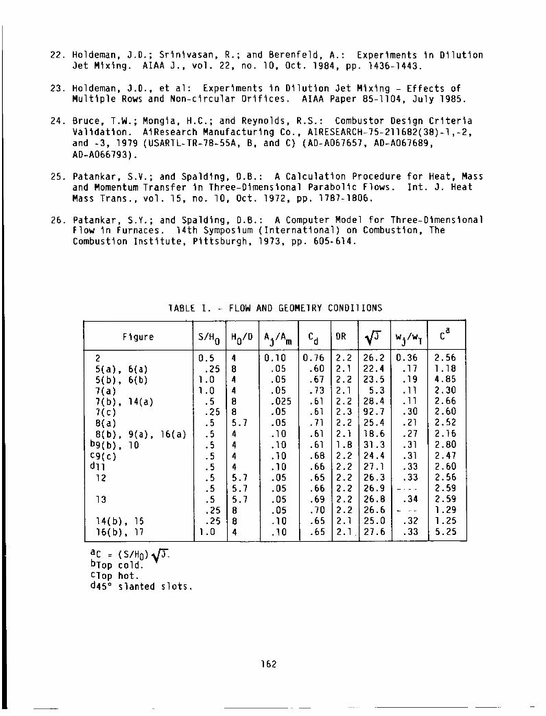
22. Holdeman, J.D.; Srlnlvasan, R.; and Berenfeld, A.: Experiments in Dilution
Jet Mixing. AIAA J., vol. 22, no. lO, Oct. 1984, pp. 1436-1443.
23. Holdeman, J.D., et aT: Experiments in Dilution Jet Mixing - Effects ofMultiple Rows and Non-clrcular Orifices. AIAA Paper 85-II04, July 1985.
24. Bruce, T.W.; Mongla, H.C.; and Reynolds, R.S.: Combustor Design Criteria
Validation. AIResearch Manufacturing Co., AIRESEARCH-75-211682(38)-l,-2,
and -3, 1979 (USARIL-TR-78-55A, B, and C) (AD-A067657, AD-A067689,
AD-A066793).
25. Patankar, S.V.; and Spalding, D.B.: A Calculation Procedure for Heat, Massand Momentum Transfer in Three-Dimenslonal Parabolic Flows. Int. J. Heat
Mass Trans., vol. 15, no. lO, Oct. 1972, pp. 1787-1806.
26. Patankar, S.Y.; and Spalding, D.B.: A Computer Model for Three-DimenslonalFlow in Furnaces. 14th Symposium (International) on Combustion, The
Combustion Institute, Pittsburgh, 1973, pp. 605-614.
TABLE I. - FLOW AND GEOMEIRY CONDITIONS
Figure
2
5(a), 6(a)5(b), 6(b)
7(a)7(b), 14(a)
7(c)8(a)
8(b), 9(a), 16(a)
bg(b), I0
C9(c)dll
12
13
14(b), 15
16(b), 17
an = ( _lH,_% ,,l_"
ip,-...o,v--b o cold.
Clop hot.d45 ° slanted slots.
SIH 0 Ho/D
0.5 4.25 8
l.O 4
l.O 4
.5 8
.25 8
.5 5.7
.5 4
.5 4
.5 4
.5 4
.5 5.7
.5 5.7
.5 5.7
.25 8
.25 8
1.0 4
Aj/A m Cd
0.I0 0.76
.05 .60
.05 .67
.05 .73
.025 .61
.05
.05
.lO
.lO
.lO
.lO
.05
.05
.05
.05
.TO
.lO
DR _J- wj/w T Ca
2.2 26.2 0.36 2.56
2.1 22.4 .17 l.18
2.2 23.5 .19 4.85
2.1 5.3 .ll 2.30
2.2 28.4 .ll 2.66.61 2.3 92.7 .30 2.60
.71 2.2 25.4 .21 2.52
.61 2.1 18.6 .27 2.16
.61 1.8 31.3 .31 2.80
.68 2.2 24.4 .31 2.47
.66 2.2 27.I .33 2.60
.65 2.2 26.3 .33 2.56
.66 2.2 26.9 .... 2.59
.69 2.2 26.8 .34 2.59
.70 2.2 26.6 .... 1.29
.65 2.1 25.0 .32 1.25
.65 2.1 27.6 .33 5.25
162
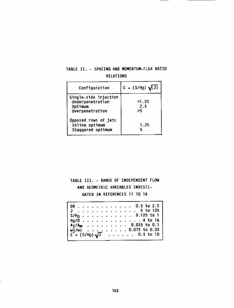
TABLE II. - SPACING AND MOMENTUM-FLUX RATIO
RELATIONS
Configuration C = (S/Ho)(_
Single-slde injection
Underpenetratlon
OptimumOverpenetratlon
Opposed rows of Jets
Inline optimum
Staggered optimum
<l. 25
2.5>5
l.25
5
TABLE III.- RANGE OF INDEPENDENT FLOW
AND GEOMETRIC VARIABLES INVESTI-
GATED IN REFERENCES 17 TO 19
DR ............ 0.5 to 2.5J ............. 5 to I05
S/H 0 ........... 0.125 to l
Ho/D ............. 4 to 16
Aj/Am ......... 0.025 to O.l
wj/wT ......... 0.075 to 0.33C = (S/Ho)_J_" ...... 0.5 to lO
163
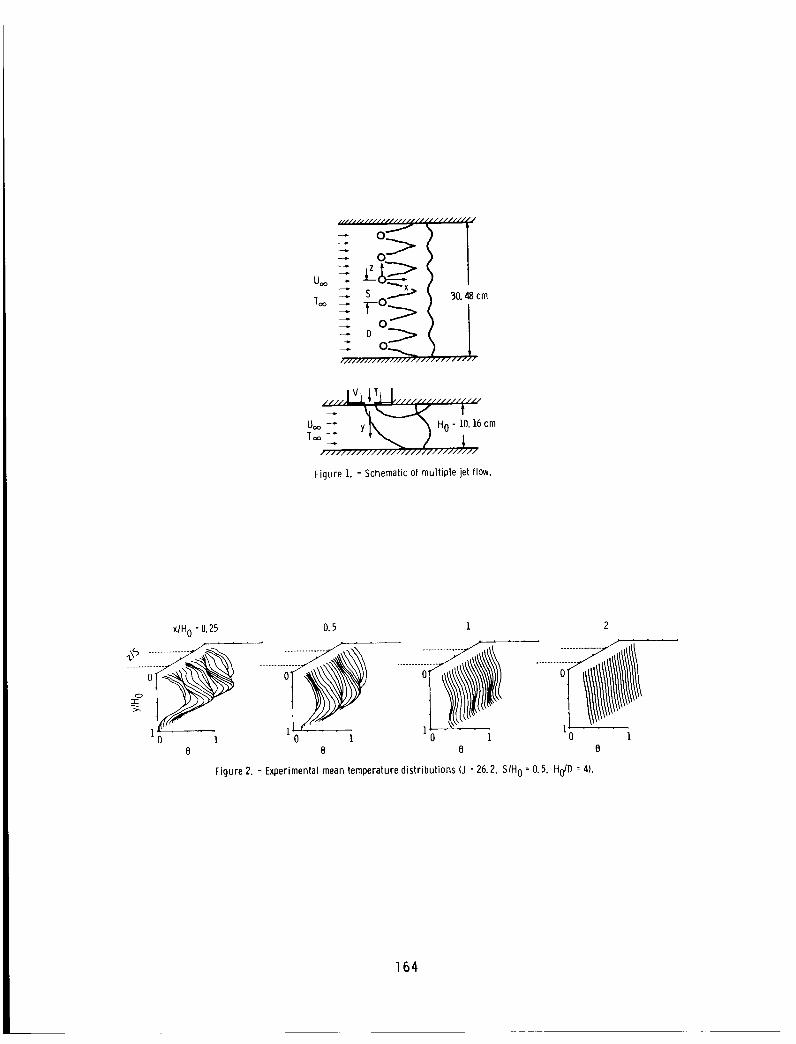
Uoo
T_o
,I, II_/IJJJHJ/J///////IA
_ s ....Z._
I//////I////////////
,ll//I/J/]
30.48cm
,1"////////
,.,.,,.lVi_Ti L,,,:,,, ...... ,,,,
Uoo _ y_'_ HO :IO.16cm
Figure 1. - Schematic of multiple jet flow.
x_/H0 : 0.25 0..5 1 2
........................"0 1
B e e e
Figure 2. - Experimental mean temperature distributions (J : 26.2, S/H0 =0. 5, H0/D : 4).
164
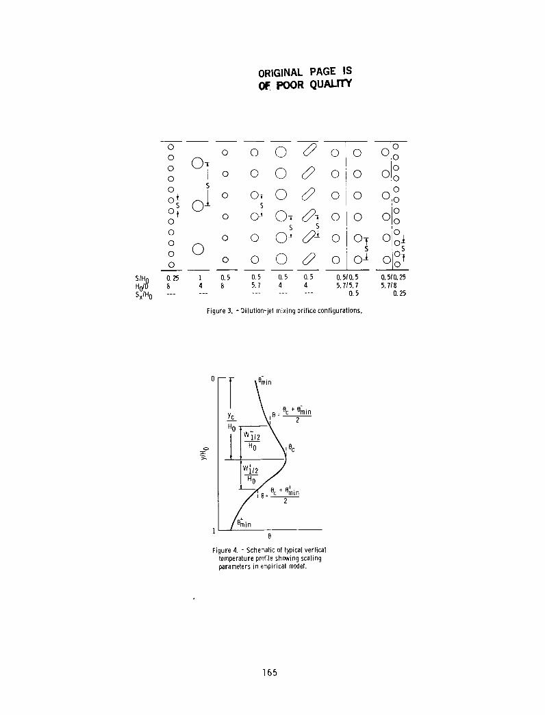
ORIGINAL PAGE IS
OF. POOR QUALITY
0
0
0
0
0
0_-
o;©
0
0
©
0
o o 0 JP oO] o o 0 J_ o
S
olO o, 0 <P oo o-_ O, 4P_ro
S S
o o 0_- o0
o o 0 4P o
o O!°oo Oo°o O°oo o °
I
o_ o°_o] oo-f
S/H0 0.25 1 0.5 0.5 0.5 0.5 0,510.5Ho/D 8 4 8 5.7 4 4 5.715.7SxlH0 ............... 0. 5
Figure 3. - Dilution-jet mixing orifice configurations.
O.510.255.718
O.25
[ tinrain
Figure 4. - Schematicof typicalverticaltemperature profile showing scalingparametersin empirical model.
165

0c_
8
u
,_1r o
.._ .-A
•-r- .o
i
166
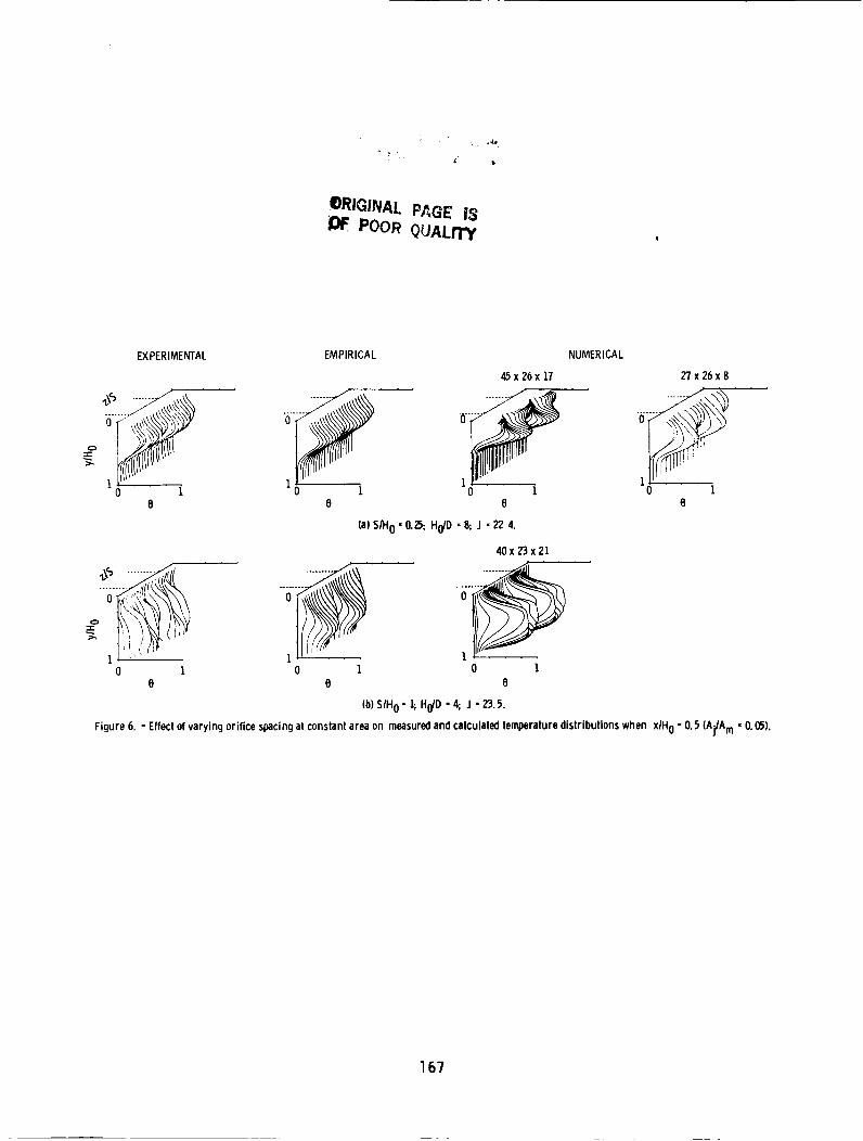
eRIQlr_AL P_,GE isPOOR QUALITY
EXPERIMENTAL
o---i
8
o :i '_\"_
0 16
EMPIRICAL
0 Ie
45x26x 17
1o i6
(a) SIH0 - 0.25; Ho/D =8; J - 22 4.
10 1
0
40 x 23 x 21
o i6
(b) SlH0 = 1; Ho/D- 4; J • 23.5.
NUMERICAL
27x25x8
0 1e
Figure 6. - Effect of varying orifice spacingat constantarea on measuredand calculatedtemperaturedistributionswhen xlH0 - O.5 (AjlAm - O.C5).
167

ORIGINAL PAGE IS
OF POOR QUALITY
0 ie
(a)SIH0 =];H0/D-4;AjJAm =0.05;J °5.3.
_ o
iil ,I :_il
(b) SIH0 " 0.5; Ho/D =8; Aj/Am - 0.0_5; J - 28.4.
0
-0.5 1.5z/S
;.ii I I;_i:;t i i:!i_:j j ti;_i• ..;::::::.?
(c)SIH0 -0.25;H0/D=8;AjlAm =0.05;,J = 92.7.
Figure l. - Obliqueprofile plots and isotherm contours when xIH0 - 0.5 for coupled orifice spacingand momentum-fluxratio.
168

ORIGINAL PAGE IS
POOR QUALITY
EXPERIMENTAL EMPIRICAL NUMERICAL
35 x 33 x 17
Z _ 4; ;;/,f">, , h/,;,k "_''
]/,//mI; 1 1
(a) Ho/D : 5.7; AjlA m : 0.05; J : 25.5.
45 x 23 x 19
I i' v,,, 1 "
0 I 0 i 0 1
0 B
(b) Ho/D : 4; Aj/A m = 0. 10, J : 18.6.
Figure 8. - Effect of varying orifice diameter at constant spacing on measured and calculated
temperature distributions when x/H 0 : 0. 5 (SIH 0 = 0. 5).
/
1 _- . !
1,L0 1
0
x/H0 : O.5 I
1 1
(a) Isothermal mainstream; J : 18.6.
_-d (2>o....
1 1
(b) Top cold; J : 31.3.
<DTI
e
(_ ......
C>6_,I0 1
B
(c) Top hot; J = 24. 4.
2
...... jJ_
,I
o ie
Figure 0. - Influence of nonisothermal mainstream on measured temperature profiles (S/H 0 = 0.5; Ho/D - 4, AjlA m ° 0. 10).
169
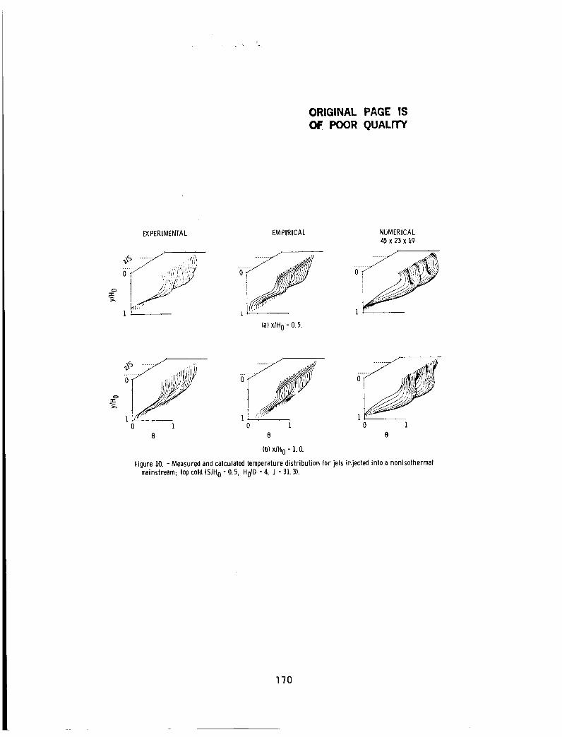
ORIGINAL PAGE IS
OF POOR QUALITY
EXPERIMENTAL EMPIRICAL NUMERICAL45 x 23 x 19
(a) x/H0 : 0.5.
....... ,111, 6-o_I_! _ or" )))li_liii_/(ii_
0 1 0 1 0 1
0 0 0
(b)xlH0 - I.O.
Figure 10. - Measuredand calculated temperature distribution for jets injected into a nonisothermalmainstream; top cold (SIH0 =0.5, Ho/D =4, J - 31.3).
170
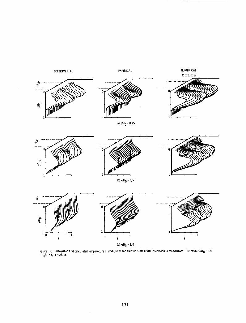
EXPERIMENTAL EMPIRICAL NUMERICAL
4.5x 23 x 19
0,
1
(a)xlH0 - O.25
0
1 1,
(b)x/H0" 0.5
1 l[ / 1o i o i o i
6 S e
(c) xlH0 - 1.0
Figure 11. - Measuredandcalculatedtemperaturedistributionsfor slantedslotsat an intermediatemomentum-fluxratio(S/H0 =O.5,Ho/D =4, J =27. 1).
171

EXPERIMENTAL EMPIRICAL NUMERICAL
36 x 29 x 19
0- 0
1 1 1
(a) x/H 0 = 0.5.
......_ o.....f o .... 6....1 1 1
0 1 0 1 0 10 0 0
(b) x/H 0 : 0. 75.
Figure 12. - Measured and calculated temperature distributions for double row of inline jets at an
intermediate momentum-flux ratio (A:/A m = 0. 10, Sx/H 0 = 0.5. Row 1: SIH 0 = 0.5, H0/D =.5.7,
J :26.3. Row2: SIH0 =0.5, H0/D =I.7, J :26.9).
EXPERIMENTAL EM PIRICAL NUMERIC AL
41 x 23 x 21
......_ .--- .._---e< ....... o o-6--
1 1 I
(a)xlH0 = 0.25.
.....___:__ .......-_-
......_ -o--_ ....'o....1 1 ]
(b) xlH 0 = 0. 5.
11
8
117 yo "0 1 1
0 B
(c)xlH0 = I.0.
Figure 13. - Measured and calculated temperature distributions for double row of dissimilar jets at an
intermediatemomentum-flux ratio(A:IAm = O.10, SxlH0 = 0.25. Row I: SIH0 = 0.5, Ho/D = 5.7,
J =26.8. Row2: SIH0= 0.25,H0/D-JS, J :26.6).
172

ORIGINAL PAGE IS
.OF. POOR QUALITY
i?:'::i!ii
I I!i!:I I:
::I I I!
!!'L-I--I::::,?_.q I I?::i
5:,htltJ/:
xlH0 =O.5 1
(a) Single-side (top)injection: S/H0 : 0.5; Aj/A m = 0.025; J =28.4.
_:____-::......_ _,_ _>_SlIII1.......c:g>-----i-_.f' c_ ......
0 1 0 16 e
2
B
(b) Opposedrow (inline) injection: S/H0 =O.25; AjlAm = O.10; J : 25. O.
Figure 14. - Comparison betweensingle-side and opposed-jet injection (Ho/D =8).
EXPERIMENTAL EMPIRICAL NUMERICAL
45 x 26 x 17
........ \)x•" .........:0 _', '_J'OK ,.,..._Y/i, J. _>'__.,,,'_i)_ ;_"
:z: ] :.L( : "_',_::f
...._!-S'" ---:t ..........(a)x/H0 = O.5.
_ ; !!!!!!!!i!!))>_,!!',:',_1
.......i-F-/(I:"0 i
......... :7"" \\ \j,_.......... .......o::::.........o _,i,,ii!i
......:-I::::)'"', "......:o : o i
e
(b)x/H0 =1. O.
Figure 15. - Measuredand calculated temperature distributions for opposedrows of inline jets (S/H0 " O.2.5, Ho/D =8,
AjlA m =O.10, J =25).
173

xlH0 = O.5 I
:i,I t t,;i; (22>d- (22, -1 i I!_
:-_:1 I Ii!::!:2:;iJ I
(a) Single-side (top) injection: SIH 0 : 0.5; J - 18.6.
2
(1_ ......J
.:: I I I II I I I ',i
.. i I I I :
ii_t I I _L__L _P.... _ ......0 0
0 1
B
(b) Opposed row (staggered) injection: S/H 0 = 1; J : 27.6.
Figure 16. - Comparison between single-side and staggered jet injection (H0/D : 4, Aj/A m : 0.10).
EXPERIMENTAL EMPIRICAL NUMERICAL22 x 27 x 33
.............. ........F F
(a) xlH 0 : O.5.
__.._i_........._,
.......... -i"
0 I
0
0 I 0 1
B B
(b)xlH0 : I.O.
Figure 17. - Measured and calculated temperature distributions for opposed rows of staggered jets (SIH 0 : 1, H0/D = 4,
Aj/A m : 0.10, J : 27.6).
174
N87-20277
THEORETICAL KINETIC COMPUTATIONS IN COMPLEX REACTING SYSTEMS
David A. Blttker
NASA Lewis Research Center
Cleveland, Ohio
This paper describes NASA Lewis' studies of complex reacting systems at
high temperature. The changes which occur are the result of many differentchemical reactions occurring at the same time. Both an experimental and a
theoretical approach are needed to fully understand what happens in these sys-tems. The latter approach is discussed herein. We present the differential
equations which describe the chemical and thermodynamic changes, and wedescribe their solution by numerical techniques using a detailed chemical
mechanism. Several different comparisons of computed results with experimen-
tal measurements are also given. These include the computation of (1) species
concentration profiles in batch and flow reactions, (2) rocket performance innozzle expansions, and (3) pressure versus time profiles in hydrocarbon igni-
tion processes. The examples illustrate the use of detailed kinetic computa-tions to elucidate a chemical mechanism and to compute practical quantltles
such as rocket performance, ignition delay times, and ignition lengths in flow
processes.
INTRODUCTION
For many years Lewis has been studying complex, reacting gas-phase sys-
tems at high temperature. The changes that occur in such systems are the
result of many individual chemical reactions occurring at the same time. We
use a two-step approach to understand what happens in such a system: (1)
experimental measurement of the temporal changes in temperature, pressure, or
composition of the system, and (2) theoretical computation of these changes in
an attempt to match the experimental results. This report describes our work
in the computation of complex-system chemical kinetics as focused on combus-
tion systems. Brabbs describes our experlmental efforts in his paper for this
symposium. Early attempts to compute the progress of complex reactions
involved various simplifications. These were of two types: (1) one or two
global reactions were substituted for the actual set of many individual,simultaneous reactions which occur in a gaseous system with several species
present, and (2) reactions involving some of the very reactive atoms and radi-cals were assumed to be very fast and, therefore, always in chemical equilib-
rium. Differential equations for the rates of change of a few key specieswere solved analytically. Although both of these approaches have had limited
success, they only explain some of the general features of a complex reaction.They are, at best, simplified approximations of the actual process, which are
only valid under a limited set of conditions. The most fruitful approach to
complex kinetics computations is to numerically integrate a system of differ-
ential equations derived from the laws of conservation of mass, energy, and
(if flow is involved) momentum. These differential equations involve the
rates of change of species concentrations _I (moles per unit mass of mix-ture) and temperature T, and they may also involve density p and velocity
V for a flow process. When these differential equations are solved, a set of
individual reactions is assumed to occur simultaneously among all the species,
and these reactions are usually assumed to be reversible (with the ratio of
175

the forward to reverse rate constant being equal to the equilibrium constantfor any reaction).
There are two ways to use these detailed kinetic computations. First,
they may be used to elucidate a reaction mechanism or to determine a single
unknown rate constant in conjunction with experimental data. On the other
hand, they may be used wlth a known mechanism to compute practical combustion
quantities such as
(1) Kinetic rocket or jet engine performance(2) Compos_tlon of engine exhaust gases
(3) Ignition delays in combustible mixtures
(4) Ignition lengths and nozzle performance in supersonic combustion
Examples of some of these computations performed at NASA Lewis are given laterin this paper.
GENERAL THEORY
A reacting system contaln_ng NS species is assumed to have NR inde-
pendent chemical reactions proceeding simultaneously. The general set ofreactions is written
NS NS
i:I k_j_ i:I
j=l,2,..., NR
Using the law of mass action, we can write the forward and reverse rate ofeach reaction as
NS
Rj = kj I-I (poi)i=l
(i)
NSI
R_j = k_j I-I (p_i) vlji=l
(2)
where p is the mass density of the mixture and oI the concentration of
species Si, (moles per unit mass of mixture). The rate constant for the for-
ward reaction kj is written in the modified Arrhenlus form
n -Ej/RTkj = AjT Je (3)
I76
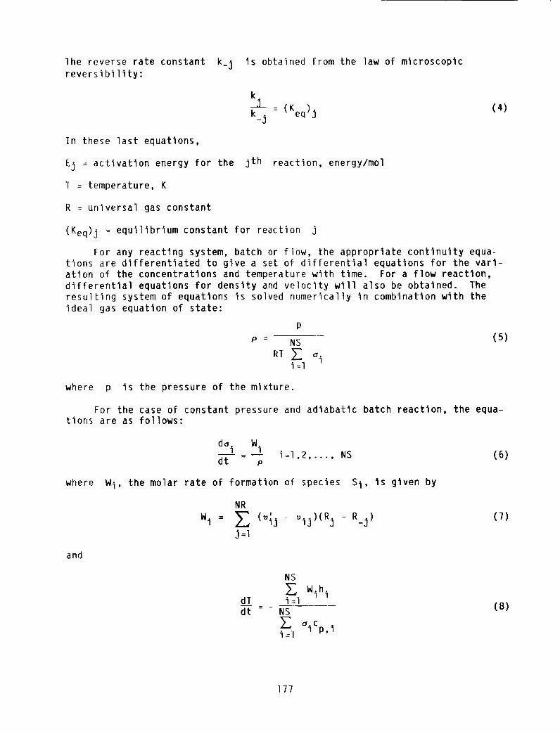
lhe reverse rate constant k_j is obtained from the law of microscopicreversibility:
k
-J-: (K)jk_.j eq
(4)
In these last equations,
Ej = activation energy for the jth reaction, energy/mol
1 = temperature, K
R = universal gas constant
(Keq)j = equilibrium constant for reaction j
For any reacting system, batch or flow, the appropriate continuity equa-tions are differentiated to give a set of differential equations for the vari-
ation of the concentrations and temperature with time. For a flow reaction,
differential equations for density and velocity will also be obtained. The
resulting system of equations is solved numerically in combination with the
ideal gas equation of state:
P : NS (5)
where p is the pressure of the m_xture.
For the case of constant pressure and adiabatic batch reaction, the equa-tions are as follows:
d_i W Ii=l,2,..., NS (6)
dt - p
where W i, the molar rate of formation of species Si, is given by
NR
Wi = _ (v_j - _ij)(Rj - R_j)
j:l
(7)
and
NS
_'_ Wih idT i=l
: - NS
_,CI p,i
i=l
(8)
177
where
hi = molar enthalpy of species Si
Cp, i = molar heat capacity of species Si
lhe standard Runge-Kutta or other explicit numerical techniques cannot be used
to solve these equations. Although the differential equations are inherentlystable, they have widely different time constants for relaxation to their
final equilibrium solution. Therefore, the step sizes required for solution
stability are prohibitively small. These systems of equations are calledstiff, and the problem of solving them accurately has been studied for many
years. Several new implicit integration methods have been developed for solv-ing these stiff equations. Although they have been quite successful in
improving the accuracy and efficiency of the solutions, there is still a need
for additional development of better methods. Problems of accuracy and of
efficient step-slze selection can still arise. Methods need to be developed
for automatic selection of the optimum integration parameters. Therefore,
research is actively proceeding at many institutions to develop more efficientintegration methods (refs. l to 4).
There is another kinetic combustion model of interest to practical enginedesigners - namely, highly backmlxed reacting flow in what is usually called
the well-stlrred reactor. We assume the limiting condition of zero-dlmenslonal
flow or instantaneous backmlxlng of the reacted gases with the cold, unreacted
gases. Although this model is an oversimplification of highly turbulent
reacting flow, it is a very useful first-order approximation for some practi-
cal reactlng-flow systems.
The process is a constant pressure combustion with mass flow rate
through a reactor of constant volume v. The average residence time in thereactor is
pvt =r &
(9)
For each species we can write a continuity relation which says the fol-lowing: The difference between the species molar flow rate into and out of
the reactor is equal to its rate of formation (or destruction) by chemical
reaction in the reactor. These continuity equations are
NR
& (oI ) ' _v - + (vlj vlj)(R j - R j)
j=l
I=1,2,..., NS (lO)
The following energy conservation equation can also be written (if we assumethat the process is adiabatic):
NS
(alhl * *) = 0I=I - _lhl
(ll)
In these equations * indicates the unreacted gas mixture. Equations
(lO) and (ll) are a set of nonlinear, algebraic equations for _I and the
178
reactor temperature. They are solved by the Newton-Raphson lterattve proce-dure. Logarithmic increments of the variables are used to avoid numericalproblems (ref. 5).
NASA GENERAL CHEMICAL-KINETICS CODE
Many computer codes have been published which perform different kinds of
chemlcal-klnetlc computations. At NASA Lewis we published a general chemical-
kinetics code, GCKP84 (ref. 6). It performs a wide variety of chemical-
kinetics computations with convenience and efficiency.
It is designed to perform chemlcal-klnetlcs computations for severalreaction models, including the following:
(I) General reaction In either a batch system or a one-dlmenslonal,frlctlonless plug flow
(2) Combustion reaction In a well-stlrred reactor (highly backmlxed flow)(3) Reaction behind a shockwave wlth boundary layer corrections
(4) Ignition processes In either a batch or flow system(5) Nozzle expansion reactions
For each of these models the following general features of the code apply:
(1) Any chemical system may be used for which reaction rate constant data
and species thermodynamic data are known.
(2) The process may be adiabatic, or the heat transfer between thereaction and Its environment may be considered.
(3) A new efficient integration technique is employed (ref. 7).
(4) Any chemical reaction of the form aA + bB_dD + eE may be used,including photochemical and ionic reactions.
(5) Simplified input for combustion reactions may be used.
The code contains an option to compute rocket performance parameters for
nozzle flow and can be conveniently used to compute ignition lengths In super-
sonic flow. An option Is also provided to perform a well-stlrred reactor
computation and, then, immediately expand the products through an assigned
nozzle profile.
EXAMPLES OF CHEMICAL KINETIC COMPUTATIONS WITH GCKP84
Hydrogen-Oxygen Batch Reaction at Constant Temperature
Measurements of hydrogen peroxide formation In the constant-volume, iso-
thermal reaction of hydrogen and oxygen at 500 °C were reported many years ago
by Baldwin (ref. 8). The important reactions In the hydrogen-oxygen mechanismare as follows:
H2 + 02 = OH + OH
179

H2 + OH = H20 + H
H + 02 = OH + 0
0 + H2 = OH + H
*H + 02 + M = HO 2 + M
H + HO2 = OH + OH
*H202 + M = OH + OH + M
*HO 2 + HO2 = H202 + 02
*H2 + HO 2 = H202 + H
The rate constants for many of these reactions have been measured fairly
accurately, but some of the reactions involving H202 and HO 2 still have a sig-
nificant uncertainty. The reactions important in determining H202 concentra-
tion are indicated by an asterisk. GCKP84 was used to compute the H202 versus
time profile. After making several variations of the rate constants for the
two most uncertain and important reactions (H2 + HO 2 _ H202 ÷ H and HO2 +
HO2 _ H202 + 02), we obtained the agreement between the experimental and com-puted results shown in figure l. This example illustrates the use of kineticscomputations in obtaining better rate-constant values for one or two key reac-tions when all other reactions in a mechanism are fairly well known. Of
course, we cannot say that we have uniquely determined both reaction rate con-
stants since we have two adjustable parameters. But we have put limits on
their uncertainty. Of course, this type of exercise can only be done when the
experimental variable being matched by computation is sensitive to small vari-ations in the uncertain rate constants, lhls brings up the following general
question: For a given change in any rate constant of the reaction mechanism,how much does each computed variable change? This is the relatively new
field of study in chemical kinetics called sensitivity analysis.
In practice, even through a chemical mechanism may contain more than lO0reactions, only the rate constants of 15 or 20 may significantly affect the
computed results when their values are changed. Recently, methods have been
developed to systematically compute these effects in the form of sensitivity
coefficients (refs. 9 to ll). This computation is performed along with the
chemlcal-klnetlcs computation. The results of the latter computation are used
as input to solve a second set of differential equations whose unknowns are
sensitivity coefficients of the form
kR ac I(12)
SiR - cl ak R
2
kRk m a ci(13)
TiR m - cl akRak m
The flrst-order coefficient SiR effectively gives the percentage change in
ci (Ith concentration variable) for a given percentage change in the rateconstant of reaction _. The second-order coPfflclent TIRm gives the effect
180

on cI of changes in both k_ and km. It is now recognized that a sensi-
tivity analysis must be performed for any complex reaction in order to pinpointthe important reaction paths and obtain a good understanding of the reactionmechanism.
Computation of Rocket Performance
One of the first uses of chemical kinetic computations was in the compu-
tation of rocket performance using a one-dimensional flow model. This per-
formance is measured by the velocity of the hot gas at the nozzle exit point.
As the gas expands and cools, its velocity (i.e., kinetic energy) is kept ashigh as possible by chemical recombination reactions which occur in the noz-
zle. These reactions convert high-potential-energy atoms and radicals into
low-energy stable molecules. Maximum performance is obtained if these reac-
tions maintain equilibrium conditions in the very short nozzle-resldence time.But this is often not the case since the finite rates of the reactions are not
fast enough. By knowing the rate constants for the important recombination
processes one can compute kinetic performance that more accurately and realls-
tically reflects the experimentally measured performance. An example of this
is shown in figure 2 for the oxygen difluoride - dlborane system (ref. 12).
The three curves of performance as a function of oxldant/fuel ratio (fig. 2(b))
show the maximum and minimum theoretical performance (assuming equilibrium andfrozen conditions) as well as the kinetlcally limited performance. The latter
agrees rather well with actual measurements corrected for various losses. The
reaction mechanism used is shown in table I. This system is interesting
because only one reaction rate constant has to be accurately known in order to
compute the kinetic curve. This is the recombination of hydrogen atoms to
give molecular hydrogen. This fact was determined by a simple sensitivity
analysis. Computed performance is unchanged for wide variations of the otherrate constants. The reason for this situation can be seen fromthe heat
release data in table I. The hydrogen atom recombination accounts for well
over 50 percent of the heat release in the process, and this, of course, con-trols performance.
Two-Stage Well-Stirred Reactor
The practical use of the well-stlrred reactor model of GCKP84 is illus-
trated by its simulation of a two-stage turbulent combustor. A theoretical
and experimental study of two-stage, rich-lean combustion as a method of con-
trolling nitrogen oxide emissions was performed at Lewis. This technique was
suggested as a way of reducing the conversion of the organic nitrogen compounds
in hydrocarbons (fuel-bound nitrogen) to nitric oxide during combustion. The
objective of the work was to study the effect of operating conditions on emls-
s_ons of both nitrogen oxides (NOx) and carbon monoxide (CO) (ref. 13).
Both the nitrogen and the hydrogen content of the fuel were changed to simu-late coal-derlved syncrude fuels, lhese fuels contain high percentages of
aromatic hydrocarbons and therefore have a lower hydrogen-to-carbon ratio than
today's petroleum-based fuels. Experiments were performed in the two-stage
flame-tube apparatus shown in figure 3. lhe fuels were mixtures of propane,
toluene, and pyrldlne blended to give a range of hydrogen and nitrogen con-tents. The prlmary-zone equivalence ratio was varied from 0.7 to about 1.8.
lhe products of flrst-stage combustion were rapidly diluted with air injection
181

and burned at a final equivalence ratio of 0.5. The final NOx and COconcen-trations were measured. The two-stage flame tube was modeled analytically bya two-stage stlrred-reactor computation closely simulating the experimentalfuels. Instantaneous mixing of the secondary dilution air was assumed. Adetailed chemical mechanismwas used for propane and toluene oxidation and forNOx formation. The fuel-bound nitrogen was input as nitrogen atoms and allmixing and heat-transfer effects were neglected. This very simplified modelof a quite complex process was able to predict most of the observed trends ofNOx and COformation with variation of nitrogen and hydrogen concentrationsin the fuel. The model's prediction of other trends, which were not measuredexperimentally, gave additional information about the advantages and disadvan-tages of using this rlch-lean combustion for emissions control. A comparisonof someexperimental and computedresults for NOx and COconcentration as afunction of primary equivalence ratio is given in figures 4 and 5. The simplemodel qualitatively predicts the observed trends. It can be seen that using arich primary equivalence ratio does reduce NOx formation very significantly.However, at the sametime, this technique increases the formation of CO,whichis also undesirable. Thus, one set of conditions cannot minimize both pollut-ants, and tradeoffs will have to be madeto obtain desired emissions levelsfor any practical situation. This work has shownthat a simple kinetic modelcan sometimesbe used to qualitatively explain the observed trends in a highlycomplicated combustion system.
Ignition Delays in Benzene-Oxygen-ArgonMixtures
Our current work involves the study of the mechanismof hydrocarbon oxida-tion. Weare studying the allphatlc hydrocarbons by measuring ignition delaysand concentration profiles during the shock-heated oxidation of hydrocarbon-oxygen-argon mixtures. Then a detailed chemical mechanismis formulated andused in detailed kinetics computations to match the observed experimental dataover a wide range of initial composition, temperature, and pressure. Wearealso studying the simplest aromatic, benzene. A partial mechanismfor benzeneoxidation is as follows:
C6H6 + 02 = C6H5 + HO2
C6H6 = C6H5 + H
C6H6 = C4H4 + C2H2
H + 02 = OH+ 0
H ÷ 02 + M = HO2 + M
0 ÷ C6H6 = C6H5 + OH
OH÷ C6H6 = C6H5 + H20
C6H5 ÷ 02 = C6H50+ 0
C6H50+ M = C5H5 + CO+ M
CO÷ OH= CO2 + H
182

The experimental program is described by T.A. Brabb's paper presented at thtssymposium. I attempted to match experimental ignition delay data for benzene-oxygen-argon mixtures that were taken by another investigator at Lewis. Thereaction zone behind the experimental reflected shock Is approximated by aconstant volume batch reaction. The theoretically computed temperature andpressure (for nonreacttng conditions) behind the shock are used as startingconditions. A typical, computed profile of pressure as a function of ttmetsshown tn figure 6. The Ignttlon delay _ ts determined from the first sig-nificant pressure rise; this ts similar to determining the experimentalvalue from the measured pressure trace. The mechanism we used includes over100 reactions Involving benzene and tts degradation products, acetylene, phe-nol, phenylacetylene, ethylene, and methane. It includes a11 the reactions ofthe hydrogen-oxygen system as well. Values from the literature were used forall reaction rate constants except the qutte uncertain ones of the benzene,phenol, and phenylacetylene reactions. These were varied within reasonable
limits to get the best overall agreement between computed and experimentalT values. Starting mixture equivalence ratios ranged from 0.5 to 2, tempera-tures ranged from about 1200 to 1700 K, and initial pressures ranged from 2 to6 arm. A simple sensitivity study made by changing rate constants one at attme has shown that the _ values are most sensitive to the rate constant forthe C6H5 + 02 reaction, which ts quite uncertain. Other rate constants which
are uncertain and have a significant effect are those for C6H6 _ C4H4 + C2H2and C6H5 _ C4H3 + C2H2. In figure ? we show some comparisons between com-puted and experimental ignition delays. We have used only the experimentaldata points which are considered the most accurate for the mechanism matching.These are the data with T values of 100 msec or greater. Shorter ignitiondelays may have significant error due to the nonunlformlty of the reactionmixture and the heating effects. The computed line for log • versus I/Tcomes within ±50 percent for all but one point which differs by about a factorof two. Whtle thts mechanism does fairly well, tt Is certainly not completeand has two significant problems. First, tt tends to predict delays longerthan the experimental ignition delays for the lean mixtures and shorter thanthe experimental delays for the rtch mixture. Second, It does not predict theexperimentally observed effect of dllutton wlth argon at a constant equiv-alence ratio of 1.0. Therefore, more work needs to be done on this oxidationmechanism. A full understanding of the oxidation wt11 probably not be achieveduntil further experimental data are obtained on concentration profiles of a keyspecies, such as the phenyl radical or carbon dioxide. Work along these linesIs proceeding at Lewis and other laboratories.
REFERENCES
1. Htndmarsh, A.C.: Linear Multtstep Methods for Ordinary Differential Equa-tions: Method Formulations, Stability and the Methods of Nordsteck and6ear. UCRL-Sl186-Rev 1 Lawrence Ltvermore Laboratory, 1972.
2. Radhakrtshnan, K.: Comparison of Numerical Techniques for Integration ofStiff Ordinary Differential Equations Arising In Combustion Chemistry,NASA TP-2372, 1984.
3. Radhakrtshnan, K.: Integrating Chemical Kinetic Rate Equations by Selec-tive Use of Stiff and Nonsttff Methods. AIAA Paper 85-0237, 3an. 1985.
183

4. Pratt, D.I.; and Radhakrlshnan, K.: CREKID: A Computer Code for Tran-
sient, Gas Phase Combustion Kinetics. NASA TM-83806, 1984.
5. Pratt, D.T.: PSR-A Computer Program for Calculation of Steady Flow Homo-
genous Combustion Reaction Kinetics. Washington State Unlverslty, Dept.
of Mech. Eng., Bulletin 336, 1974.
6. Bittker, D.A.; and Scullln, V.3.: GCKP84-General Chemical Kinetics CodeFor Gas-Phase Flow and Batch Processes Including Heat Transfer Effects.
NASA TP-2320, 1984.
7. Zeleznlk, F.J.; and McBride, B.3.: Modeling the Internal Combustion
Engine, NASA RP-1094, 1985, Chapter 2.
8. Baldwin, R.R.; Rossiter, B.N.; and Walker, R.W.: Hydrogen Peroxide Yields
in the Hydrogen ÷ Oxygen Reaction. Reaction of HO2 Radicals With Hydro-
gen. Trans. Faraday Soc., vol. 65, no. 556, Part 4, Apr. 1969,
pp. 1044-I050.
9. Dunker, A.M.: The Decoupled Direct Method for Calculating SensitivityCoefficients in Chemical Kinetics. J. Chem. Phys, vol. 81, no. 5,
Sept. l, 1984, pp. 2385-93.
lO. Kramer, M.A.; Rabltz, H.; Calo, J.M.; and Kee, R.J.: Sensitivity Analysisin Chemlcal Kinetics: Recent Developments and Computational Comparisons,
Int. 3. Chem. Kinetics, vol. 16, no. 5, May 1984, pp. 559-5?8.
II. Yetter, R.; Eslava, L.A.; Dryer, F.L.; and Rabltz, H.: Elementary and
Derived Sensitivity Information in Chemical Kinetics, 3. Phys. Chem.,
vol. 88, no. 8, Apr. 12, 1984, pp. 1497-1507.
12. Bittker, D.A.: Theoretical Nonequillbrlum Performance of OxygenDifluorlde-Diborane Rocket Propellant. NASA TN D-4992, 1969.
13. Bittker, D.A.; and Wolfbrandt, G.: Effect of Fuel Nitrogen and Hydrogen
Content on Emissions in Hydrocarbon Combustion. ASME Paper 81-GT-63,
Mar. 1981.
184

TABLEI. - OF2-B2H6 MECHANISM
[Equivalence ratio = 1.63.]
Reaction
H + H +M_H2 +MBO + HF_-BOF + HH + F + M _-HF + M
H + OH + M _-H20 + MBF + OH _-BOF + H
F + H2 _ HF + H
H2 + OH _H20 + HBF + 0 _-BO + F
H + BF2 _HF + BFBO + F + M _-BOF + MBF + 0 + M_BOF + M
0 + H + M_OH + M
Total
Net reaction
rate,
percent
32.3
26.85.1
5.2
3.9
4.5
9.7
9.32.4
.3
.2
.3
lO0.O
Heat of
reaction,
AH,kcal/mole
-I04
-33-136
-ll9
-58
-32
-15
8-25
-169-160
-I02
Energy releaserate,
percent
53.1
13.9II .1
9.8
3.5
2.3
2.3
1.21.O
.7
.6
.5
lO0.O
II00_ /__I000 _"_'_'_ 30
i gO0 Qk--H202CONCENTRATION" 8001 /_/ /_/// i
70oI- / / ......... 20] I / /_" "LPRESSURE -
10
400 r- I ./_" - EXPERIMENTAL
:_0 t--/ /_ i COMPUTED
200 _--'''_'_ f I I I I I o10 30 50 70 90 UO 130
TIME, sec
Figure 1. - Computedandexperimentalresults for hydrogen-oxygenreaction.Temperature, T, 500%.
185

i
(3_
_E
IT" 4143KI P" 689kPa (I00psia_T - 3933K T - 2400K] U -61 m/sec(200ft/sec)U - 1433mlsec(4700ft/sec)U - 3658mlsec
_ESIDENCETIME_ (12000ftlsec)
(a) Rocketengineconditionsfor OFz-B2H6propellant Equivalence ratio,1.63.
4.50-- _ 4400
410 --_ 401111
390 --U 38OO--
370 --_ 36OO--
> 2.0
-- EQUILIBRIUM
__ "'_ KINETIC
--/(OIF) STOICH= 5.85
FROZEN
0 EXPERIMENTALDATA(CORRECTED)
I I I I I2.4 2.8 3.2 3.6 4.0
OXIDANT-FUELRATIO
(b) Performanceof OF2-B2H6 rocket propellant. Chamberpressure, 689 kPa (1_00psia).
Figure 2. - Oxygendifluoride-diborane(OF2-B2H6) rocketcombustion.
186

z
Z
_zz,_
S
i
!
187

2000E
z
o_ 1000
,-_ 800
w 600Z0 400
z
z 200
4000-EXPERIMENTAL
A DATA0 11%HYDROGEN
"/ _'_ <> 9_ HYDROGEN/ \_ • SRC COAL
-- \_ SYNCRUDEBLEND,-- \_. 8."_ HYDROGEN- _> 0 \\\ 0.95_FBN
; \\\ -- COMPUTEDRESULTS
\%. + ./. -°
I00 YDROGEN
so--- I I I I " "'l I I.6 .8 1.0 1,2 1.4 1.6 1.8 2.0
PRINU_RYEQUIVALENCERATIO,%
Figure4. - Effectof hydrogen content on NOx emissions. Fuel-boundnitrogen, 1. Opercent; secondaryequivalenceratio, 0.5; secondaryresidence time, _ 2 msec.
zO
Z
z
PERCENT4000 -- HYDROGEN
<>
@@@
2_ g_ 9
1000-18
8oo- ///''" o o
2=I- .ERCE K> 'v_ HYDROGEN
I00-- 0 g80--
60--
n
21 - []
iui.6
0 11[] 18
K I I I ! }.8 1.0 1.2 1.4 1.6 1.8
PRIMARYEOUIVALENCERATIO, ¢pp
Figure 5. - Effect of percent hydrogen on carbon monoxideemissions for hydrocarbon combustion. Fuel-bound ni-trogen, 0 percent; secondaryequivalence ratio, O.5;secondary residence time, z 2 msec.
188

3.2
2.4
2.0
1.63OO
I I I I I400 500 600 700 800
TIME, _ec
/
/[ :,ONmO_I' DELAY, _p
III I I I900 1000 1100 1200
Figure 6. - Computedpressure as functionof time for benzene-oxygen-argon shockignition. Initialtemperature, 1366K; equivalence ratio, _, 2.O.
1000
_- 800
600z
oZCl_
-- 400
2000--
2OO6.0
EOUIVALENCERATIO,
[] 0..5A 1.0/1 2.0
-- COMPUTEDRESULTS
.-1
..4 /2.0
d_ /x1.0
[]
"0.5
I I I I I I6.4 6.8 7.2 7.6 8.0 8.4
looO/T, K-1
Figure 7. - Ignition delay datafor benzene-oxygen-argon mixtures.
I8.8
189

N87- 20278
EXPERIMENIAL INVESTIGATION OF PILOTED FLAMEHOLDERS
C.F. Guo, Y.H. Zhang, and Q.M. XieGas Turbine Research Institute
Jiangyou County of Sichuan, People's Republic of China
Four configurations of piloted flameholders were tested. The range of
flame stabilization, flame propagation, pressure oscillation during ignition,and pressure drop of the configurations were determined. Some tests showed a
very strong effect of inlet flow velocity profile and flameholder geometry onflame stabilization.
INTRODUCTION
Pressure oscillation during the transient period from ignition to maximum
augmentation is a critical problem for the turbofan augmentor. Since this
pressure oscillation may cause fan flow to stall or surge, it is important to
know the peak pressure during augmentor ignition and to take some kind of
technical measure to reduce this peak pressure. Such a procedure is called
"soft ignition."
The combustion process in the fan flow of a turbofan augmentor is under a
severe condition. It is helpful to understand how to make use of the hot com-
bustion products in the core stream to ignite the combustible mixture in the
cold fan stream. The present research compares the capability for soft igni-
tion and the ability of different configurations of piloted flameholders to
ignite a cold fan stream.
C
F
Ga
Gf
h
M
P
p*
AP
T
SYMBOLS
pressure loss coefficient
area
alr-mass flow rate
fuel flow rate
gap height of V-gutter or peripheral length of test section
Mach number
pressure, kg/cm 2
3stagnant pressure, kg/cm
pressure drop or pressure oscillation value, kg/cm 2
temperature, °C
Igl mLA X FLW O

T* stagnant temperature, °C
V velocity, m/sec
AFR alr-fuel ratio
Subscripts:
0 upstream of flow orifice
l downstream of flow orifice or upstream of air heater
2 inlet of test section
3 outlet of test section
a air or ambient
ave average
APPARATUS
The test apparatus Is shown In figure I. The airflow from the compressorIs divided Into two streams: one stream goes to ejector 7 to create a low-
pressure exhaust condition for the test section; the other stream goes through
valve l, flow-oriflce meter 2, air heater 3, control valve 4, and plenum cham-ber 5 into test section 6. After leaving the test section the combustion
products are cooled by water injection. The hot gas Is exhausted into the
ambient through the ejector.
The test rlg assembly Is shown In figure 2. It Is a rectangular duct
300 mm by 175 mm. The piloted flameholder Is mounted inside the test section
by bolts. Flame extinction Is recorded through a quartz window by a flame-detection device. Flame extinction can also be observed visually. The igni-
tion in the primary zone is provided by a hlgh-energy ignitor of 12 J. The
combustible mixture in the secondary zone Is ignited by flame propagation from
the primary zone. The inlet flow Is measured by the static pressure tap, the
stagnant pressure tube, and the chromel-alumel thermocouple. The outlet tem-
perature Is monitored by a platlnum/platlnum-rhodlum thermocouple. Outlet
stagnant pressure Is measured by three water-cooled stagnant pressure probes;
each has three measuring points. The transient pressure is measured by an
Inductlon-type pressure transducer (CyG-l, 0 to l.O kg/cm 2) wlth an LR-I
carrier wave amplifier and an Sc-60 ultraviolet oscilloscope. The fuel flow
rate is measured by a turblne-type flowmeter wlth a digital frequencyindicator.
The fuel Is injected through a spray bar. There Is one spray bar In the
primary zone. The total length of the bar Is 280 mm. There are slx pairs ofholes (0.4 mm In dlam) on the bar at an intersection angle of 60 °. In the
secondary zone there are slx spray bars. The two bars In the center have four
pairs of holes (0.35 mm In dlam) at an intersection angle of 30°; the other
four spray bars have four holes (0.35 mm In dlam) each. Fuel injection In the
secondary zone is In the counterflow direction. The test configurations of
piloted flameholders are shown In figure 3.
192
TESTMETHOD
The test conditions were as follows:
l_ 60 to 70 °C or 500 °C
M2 0.23
P_ 0.25 to 1.2 kg/cm 2
The test procedures were as follows: First, the air supply was adjusted to
maintain the inlet conditions of P_, M2, and T_ as specified. After the
primary zone had been ignited the ejector air supply was adjusted to maintain
P_, M2, and T_ constant. Then the fuel flow in the primary zone Gfp was
increased until fuel-rlch flameout occurred. After that, the _rlmary zone wasreignited at the specified inlet condition and P_, M2, and T2 were keptconstant. Finally, the fuel flow was reduced until there was fuel-lean flame
extinction. Before ignition, the pressure drop between the inlet and outlet
was measured. During ignition the peak pressure, the fuel-alr mixture in thesecondary zone, and the pressure oscillation were also recorded.
RESULTS AND DISCUSSION
Peak Pressure Measurements
As shown in figure 4, the peak pressure rise during ignition is usually
lower than lO percent of the inlet pressure (AP2/P _ < TO percent). The
peak pressure rise in the augmentor is normally related to the amount of fuel
injected (as in these tests). Since the ignition is realized in a small vol-
ume, the amount of fuel necessary for ignition is small. Thus, the peak pres-
sure is lower than that for normal augmentor ignition. This proves that using
a piloted flameholder makes it easier to obtain a soft ignition in a turbofan
augmentor.
Pressure Oscillation Measurements
Pressure oscillation measurements were performed under the same conditionsas the peak pressure measurements. The amount of fuel injected in the primary
zone has a very strong effect on the pressure oscillation in the augmentor
during ignition in the secondary zone (figs. 5(a) and (b)). It has been shown
that, with the same amount of fuel injected in the secondary zone, the pressure
oscillation during the onset of secondary combustion varies with the amount of
fuel injected in the primary zone. It is clear that there is an optimum fuelinjection in the primary zone which minimizes the pressure oscillation during
secondary zone ignition.
Flow Resistance
Figure 6 shows the variation of the pressure loss coefficient with the
Reynolds number Re for different configurations. When Re increases, the
pressure loss coefficient C decreases slightly. The pressure loss coeffi-
cient C also decreases with the increase of gap height h. The pressure loss
coefficient C for a V-gutter is slightly lower than that for a semlspherical
shape.
193
Effect of Inlet Flow Distortion
lhe inlet flow distortion is shown in figure 7. Figure 8 shows the effectof inlet flow d_stortlon on flame stabilization. When the inlet flow is dis-
totted, the range of flame stabilization is narrowed, and the peak value of the
stabilization parameter is also reduced. For instance, at P_ = 0.25 kg/cm 2
when there is no inlet distortion, it is possible to ignite the secondary zone
in 3 sec; but, when there is inlet distortion (even at P_ = 0.3 kg/cm2), the
range of flame stabilization is very narrow and the ignltablllty in the sec-
ondary zone is very weak. (It is impossible to ignite the fuel-alr mixture inthe secondary zone.)
Effect of Secondary Air Entry Holes on Stabilizationof the SJ410-4A Flameholder
When 54 secondary holes (8 mm in diam) are opened, the range of flamestabi]izatlon is very narrow (fig. 9). When these holes are blocked, the
stabilization range is broader. The secondary air entry holes also reduce the
capability of igniting the fuel-air mixture in the secondary zone. It seemsthat the secondary air dilutes the primary combustion products and reduces the
temperature.
Effect of Gap Height
Figure lO(a) and (b) show the effect of gap height h on flame stabili-
zation for the SJ410-4B and SJ410-3A configurations. The range of flame
stabilization decreases with the increase of the gap height h, and the Ignlt-
ability also decreases. From this test we found that, for a specified con-
figuration, there is an optimum gap height. For instance, when the width of
the V gutter is ?0 mm (SJ410-3A), the optimum gap height is 3 to 5 mm, the
width of V-gutter is 40 mm (SJ410-4B), and the optimum gap height is 2 to 3 mm.
Under these conditions, the range of ignition and flame stabilization and the
ignition capability in the secondary zone are nearly the same for the two
configurations.
Effect of Bluff Body Shape on Flame Stabilization
Figure ll(a) shows the flame stabilization range for the SJ410-3A con-
figuratlon under ambient air temperature with a different bluff body shape.
lhe range of flame stabilization of the V-gutter bluff body is wider than that
of the semlspherIcal bluff body. But as shown in figure ll(b), at T_ = 500 °C
the ranges of flame stabilization for both bluff bodies are nearly the same.
Ibis can be explained as follows. At high inlet temperature, the vaporlzatlonrate of the fuel spray (before entering the primary zone) is hlgh for both
flameholders; therefore, the gaseous fuel-air ratios of the mixtures in the
primary zone are nearly the same. But at low temperature, the fuel vaporl-7_flnn r_f_ nn fh_ V_nllff:r ¢llrf_ro ic hinh_r fh_n fhmf nn fha :ami_(nharlr}l
body, and the fuel-alr ratio in the primary zone of the V-gutter is higher than
that of the seml-spherlcal body. lhus, the V-gutter has a wider range of flamestabilization.
Effect of Air Entry Holes in V-Gutter Wall on Flame Stabilization
Figure 12 shows the range of flame stabilization for the SJ410-3B con-
figuratlon with different air entry holes in the V-gutter wall. For a given
194
opening area, fewer holes with larger diameters offer better flame stabili-zation than smaller holes. A comparison of figure lO(b) with figure 12 showsthat the reclrculatlon zone created by the gap provides better flame stabili-zation than that created by circular holes.
- CONCLUSIONS
These tests led to the following conclusions.
(1) The use of a piloted flameholder in the turbofan augmentor may
minimize the peak pressure rise during ignition. At the present experimental
conditions, AP/P_ is less than lO percent; therefore, the use of a piloted
flameholder is a good method to realize soft ignition.
(2) The geometry of the piloted flameholder and the amount of fuel
injected into the flameholder have a strong effect on the pressure oscillation
during ignition of the fuel-alr mixture in the secondary zone.
(3) Compared with the V-gutter flameholder wlth holes in its wall, the
V-gutter flameholder without holes not only has the advantages such as simple
structure and good rigidity but offers a wide combustion stability limit and a
hlgh capability of igniting the fuel-alr mixture of the secondary zone.
BIBLIOGRAPHY
Branstetter, J.R.; and Juhasz, A.J.: Experimental Performance and Combustion
Stability of a Full Scale Duct Burner for a Supersonic Turbofan Engine. NASATN D-6163, 1971.
Cullom, R.R.; and 3ohnsen, R.L.: Operating Condition and Geometry Effects on
Low-Frequency Afterburner Combustion Instability in a Turbofan at Altitude.NASA TP-1475, 1979.
Kurkov, A.P.: Turbofan Compressor Dynamics During Afterburner Transients.NASA TM X-?IT41, 1975.
Marshall, R.L.; and Canuel, G.E.: Augmentation Systems for Turbofan Engines.Presented at Crafleld International Symposium, 1976.
195

7
Exhaus_
I
Air supply
W " -- 2_.,x,,,_
C _
6 5 4 3
D
Figure 1. - Test apparatus. Valve, 1; orifice flowmeter,2; air heater, 3; contro] valve, 4; plenum chamber,5; test section, 6; ejector, 7; valve, 8.
I Secondary zone 2 _ 4
Air
"IL,o _a_ ___5__l_J_ _ ___
Figure 2. - Test rig assembly. High energy ignitor, I; quartzwindow, 2; thermocouple, 3; pressure probe, 4; pressuretransducer, 5; test configuration, 6; fuel spray, 7; fuelspray bar, 8; thermocouple, 9; pressure probe, 10; pressuretap, 11.
196

I I I I { I l * ' • 1 l !i
• ' i / ' ! 1 _ 1 / / r ;
II
JI
o iq
-iJ
1/ •
(a) Configuration $3410-4A; h = 4 mm.
I / / I / ,' [ I / /. ,' t t _ / ,' {
f J I • I / I
iI
t '- i I f_ / 7 • " ! ," . 1
(b). Configuration $3410-4B; h = 2, 3, 4, and 6 mm.
Figure 3. - Test configurations of piloted flameholders.
(All dimensions in mm.)
197
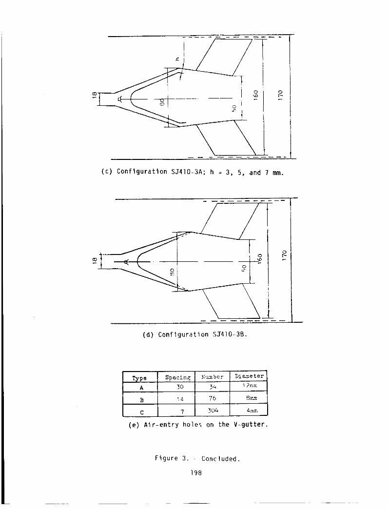
(c) Configuration SJ410-3A; h = 3, 5, and ? mm.
\(d) Configuration SE410-3B.
T_pe Spacing Number Diameter
A 30 34 12mm
B I_ 76 Bmm
C 7 3OZ_ 4mm
(e) Air-entry holes on the V-gutter.
Figure 3. Concluded.
198

_pe A B
p_ kg/cm2 I.2 O.B
_P2 Kg/c=2 0.057 0.047
n P2/F_ % 4.8 5.
C D E
0.6 O.4 O.3
0.051 0.0085 0.0085
2.5 2.1 Z.8
Figure 4. - Pressure oscillation during ignition.
199

c-
o
N
0
¢_}
t-
O
-r-
-4-'
t---
0
I
200

.... o' ....o- .'o 0 0 0 o 0cO _D _ _U _ GD
_y_Tey _On(I
o_
0
c-
O
0
oU,--
I--4
I
r"
Q)
"m
O_
(J
I
C_
aJ _
I
0 0
_UaTOTJ3OOO c_oI eun_s_ud
o
o
,?o
0
r'-
0
r"
r-
CL_--
Ln ¢.J
,4*-*
u,--_--
O_-
_P
-_ 0
"' 0
i
_P _n
-_ L
201

o
o _ _
t-O
4-J
>_ _-
4_ E_t-.r-
.,- C_) ou
0
•¢" U_ e,-- o
4._ m
e'-,_
i
0 0 0 00 0 0 0
oo
I
o _
o o o o
o o o
8
o
Q
Q;EO_Q
q..I!
c-O_
cu
_-F-0
0 J4_0
Q; e-,-- 0
_-.,-
0
4_.,-
_- 0
t_J
i_ IIN
Iii-
202

e--
o
n:l
N
0r'-
-I--.
n_
V)
(1)
E
p...-
t-
O
c-
e,-
o
_1 .! [ _
v
i
C_
r"-
S-
C)1
203

I I _ _1 . _[0 0
_a/_A
:11;
f
0
g
0
I!
I-
o
II
-Ic
F--
I
Q
el)
0
N
0 r--
.i _ e-_
•r- O_
4- E
v
II
X
o
o
F--
I
t-
O
s,-
0
e_
J_
0
0
r-
204

300 I t
@
I I300 600
AFR
Figure 12. - Effect of alr-entry holes in
V-gutter wall on flame stabilzatlon.
Configuration SJ410-3B; T2* = 500 °C,
M2 = 0.23.
205

N87"20279
THE CHEMICAL SHOCK TUBE AS A TOOL FOR STUDYING HIGH-
TEMPERATURE CHEMICAL KINETICS
Theodore A. BrabbsNASA Lewts Research Center
Cleveland, Ohto
Although the combustion of hydrocarbons ts our primary source of energytoday, the chemical reactions, or pathway, by whtch even the stmplest hydro-carbon reacts wlth atmospheric oxygen to form CO2 and water may not alwaysbe knoun. Furthermore, even when the reactton pathuay Is known, the reacttonrates are always under discussion. The shock tube has been an Important andunique tool for bulldtng a data base of reactton rates Important In thecombustion of hydrocarbon fuels.
The ablllty of a shock wave to bring the 9as sample to reactton conditionsraptdly and homogeneously makes shock-tube studies of reactton klnettcsextremely attractive. In addition to the control and uniformity of reacttoncondltlons achleved wlth shock-wave methods, shock compression can produce gastemperatures far In excess of those tn conventional reactors. Argon can beheated to well over 10 000 K, and temperatures around 5000 K are easilyobtained wtth conventional shock-tube techniques. Experiments have proven thevalldlty of shock-wave theory; thus, reactlon temperatures and pressures canbe calculated from a measurement of the tnctdent shock veloclty.
Thls report presents a description of the chemical shock tube and aux11-tary equipment and of two examples of klnetlc experlments conducted In a shocktube. Shock-wave theory and shock tubes _n general are discussed Inreferences 1 and 2 and thus are not Included In thls report.
EXPERIMENTAL APPARATUS AND PROCEDURES
The chemlcal shock tube used was a stngle piece of square stainless-steeltubing (5.7 m long, 6.4 cm on a side, 1.3 cm thick walls). The entire lengthof the tube was ground to a constant Inside dimension and then honed to ahighly polished flnlsh. Stattons for shock-wave detectors were located at15-cm Intervals In the downstream portlon of the tube. Two 2.5-cm calctumfluoride windows were located 25 cm from the end of the tube. A quartz pres-sure transducer was located at a posltlon where tt would provtde an accurateIndication of the ttme at whtch a shock wave arrived at the center of the win-dows. The assembled tube could be evacuated to a pressure of about 1 um andhad a leak rate of less than 0.2 pm/mln. A 11quid nttrogen cold trap In thevacuum line guarded agalnst the back-mlgratlon of pump oll tnto the shock tube.
The temperature and pressure behind the Incident and reflected shock waveswere calculated from the measured veloclty of the Incident shock wave with theshock program of Gordon and McBrtde (ref. 3). Since the reactton temperaturehad to be calculated, tt was very Important to measure the lnlttal temperatureand the shock velocity as accurately as possible. The distances between probelocations were accurately measured to four stgnlftcant ftgures. The shock-tubewall temperature was measured to ±0.5 C, and It was assumed that the test mlx-ture raptdly achieved this temperature. Thin-film resistance gauges (1.3 cm
207

diam) were used to detect the passage of the incident shock wave. The ampli-fied output from these gauges was displayed on a digital oscilloscope (see
fig. l). Data points were recorded every 200 nsec. Since with this scope thescale can be magnified to allow viewing of each point, we were able to measure
the incident shock velocity to better than ±0.2 _sec (O.1 percent).
All data were taken at an initial test gas pressure of B.O0 kPa (60 torr)
and a driver pressure of 792.7 kPa (ll5 psla). Soft aluminum diaphragms sepa-
rated the hlgh-pressure driver gas from the test gas. These diaphragms were
pressurized and then pierced by a gas-actlvated piston. The shock strength
was varied by adding small amounts of argon to the helium driver gas to change
its molecular weight. Figure 2 shows the variation of shock velocity with the
reciprocal of the molecular weight of the driver gas. The constant pressureratio across the diaphragm insured that the opening process for the diaphragmwas about the same for all tests.
Gas mixtures were prepared by the method of partial pressures in 34.4-
liter stalnless-steel tanks. The gases used to prepare the mixtures had stated
purities of 99.99-percent methane, 99.98-percent oxygen, and 99.998-percentargon. The partial pressure of methane and oxygen could be determined to
better than 0.3 mm of Hg, and the total pressure of the tank to better than
1.38 kPa (0.2 psla). All samples were prepared to a total pressure
of 413.6 kPa (60 psla).
Radiation at 3700 A was monitored for each experiment and was displayed
on the oscilloscope with the pressure history. The radiation was detected by
a photomultlpller tube whose field of view was restricted by two slits (0.75
and 1.5 mm wide) located lO and 23 cm from the center of the shock tube. With
this arrangement we could view a 3-mm slice of the hot gas in the center of
the shock tube at the same location as the pressure transducer. An interfer-
ence filter centered at 3696.5 A (with a half band width of ll5 A) was used toisolate the 3700 A radiation. The filter transmitted 51 percent of the inci-
dent radiation.
Examples of kinetic experiments conducted in a shock tube are presentedin the next two sections.
SHOCK TUBE MEASUREMENTS OF SPECIFIC REACTION RATES IN THE BRANCHED-CHAIN
H2-CO-O 2 SYSTEM
When a mixture containing hydrogen, carbon monoxide, and oxygen is sub-
jected to a temperature and pressure pulse in a shock tube, small concentra-tions of atoms and free radicals are first formed by processes such as
CO . 02--_C02 ÷ 0
These concentrations may then grow exponentially via the well-known branched-chain scheme
kl
OH + H2 D H20 * H
208
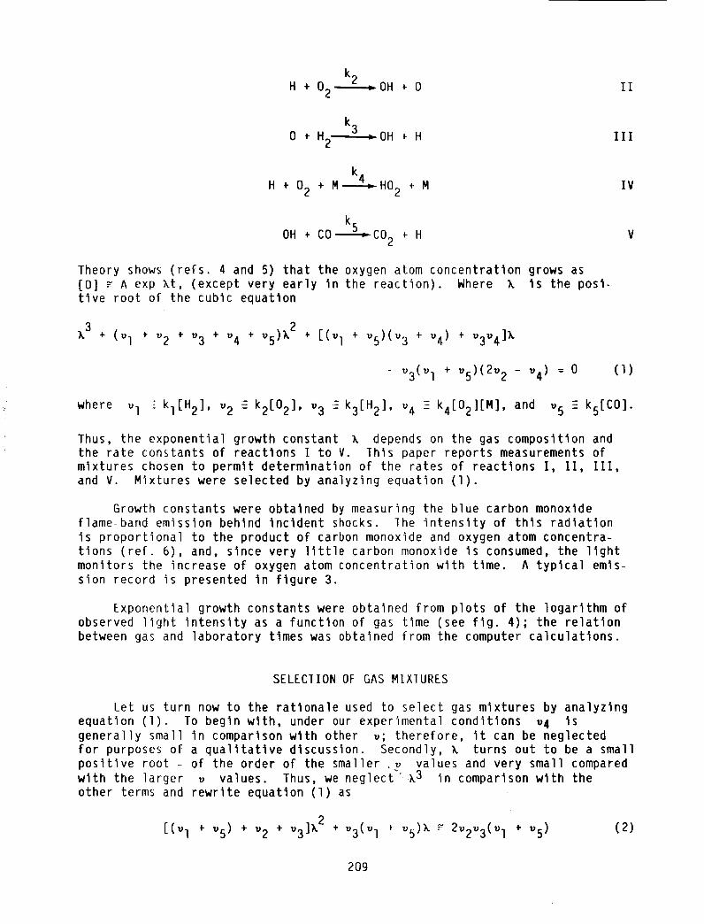
k 2H + 02 ..----_ OH _- 0 II
k 30 ÷ H2- = OH _ H III
k4
H ÷ 02 ÷ M-----_-HO2 + MIV
k5
OH ÷ CO-------CO2 _ H
Theory shows (refs. 4 and 5) that the oxygen atom concentration grows as[0] _ A exp kt, (except very early In the reaction). Where k is the posi-tive root of the cubic equation
X3 ÷ (Vl * v2 * v3 ÷ v4 ÷ v5 )k2 * [(_1 ÷ _5)(v3 _ v4) * v3v4]k
- v3(v I ÷ v5)(2v 2 - v4) : 0 (1)
where vI i£kl[H2] , v2 _ k2[02] , v3 _ k3[H2] , v4 E k4[O2][M], and v5 E ks[CO ].
Thus, the exponential growth constant _ depends on the gas composition and
the rate constants of reactions I to V. ]his paper reports measurements ofmixtures chosen to permit determination of the rates of reactions I, II, III,
and V. Mixtures were selected by analyzing equation (1).
Growth constants were obtained by measuring the blue carbon monoxide
flame-band emission behind incident shocks, lhe intensity of thls radiation
is proportional to the product of carbon monoxide and oxygen atom concentra-
tions (ref. 6), and, since very little carbon monoxide is consumed, the light
monitors the increase of oxygen atom concentration with time. A typical emis-
sion record is presented in figure 3.
Exponential growth constants were obtained from plots of the logarithm ofobserved light intensity as a function of gas time (see fig. 4); the relationbetween gas and laboratory times was obtained from the computer calculations.
SELECIION OF GAS MIXIURES
Let us turn now to the rationale used to select gas mixtures by analyzing
equation (1). To begin with, under our experimental conditions v4 isgenerally small in comparison wlth other v; therefore, it can be neglected
for purposes of a qualitative discussion. Secondly, k turns out to be a small
positive root - of the order of the smaller .v values and very small compared
wlth the larger v values. Thus, we neglect "__3 in comparison with the
other terms and rewrite equation (1) as
[(v I * v 5) + v 2 + v3]k 2 + v3(v I _ _5)k _ 2VZV3(v I ÷ v5) (2)
209
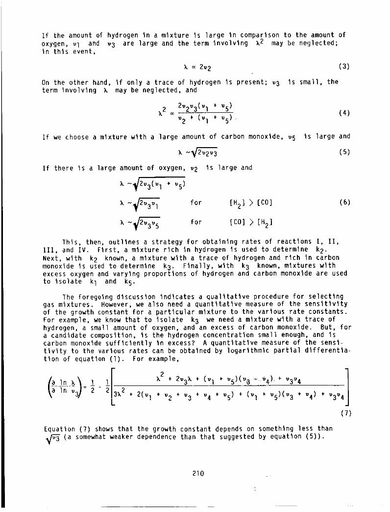
If the amount of hydrogen In a mixture Is large In comparison to the amount of
oxygen, vI and v3 are large and the term involving X2 may be neglected;In this event,
X = 2v 2 (3)
On the other hand, if only a trace of hydrogen Is present; v3 Is small, the
term involving k may be neglected, and
X2 = 2v2v3(Vl ÷ VS) (4)v2 ÷ (vI ÷ 95)
If we choose a mixture wlth a large amount of carbon monoxide, 95
If there Is a large amount of oxygen, 92 is large and
N_/293(91 + 95 )
~ 2v_ for [H2] > [C0]
X N 2_9 5 for [CO] > IN2]
Is large and
(5)
(6)
This, then, outlines a strategy for obtaining rates of reactions I, II,
III, and IV. First, a mixture rlch In hydrogen is used to determine k2.
Next, with k2 known, a mixture wlth a trace of hydrogen and rlch in carbon
monoxide Is used to determine k3. Finally, wlth k3 known, mixtures withexcess oxygen and varying proportions of hydrogen and carbon monoxide are used
to isolate kI and k5.
The foregoing discussion indicates a qualitative procedure for selecting
gas mixtures. However, we also need a quantitative measure of the sensitivity
of the growth constant for a particular mixture to the various rate constants.
For example, we know that to isolate k3 we need a mixture with a trace of
hydrogen, a small amount of oxygen, and an excess of carbon monoxide. But, fora candidate composition, Is the hydrogen concentration small enough, and Is
carbon monoxide sufficiently in excess? A quantitative measure of the sensi-
tivity to the various rates can be obtained by logarithmic partial differentia-
tion of equation (1). For example,
I x2! ÷ 293X + (91 * 95)(98 '-_4): ÷ 9394
2 X2 + 2(91 + 92 + 93 ÷ 94 ÷ 95 ) ÷ (9 ! ÷ 95)(93 , 94 ) ÷ 9394
(7
Equation (7) shows that the growth constant depends on something less than
I_-_ (a somewhat weaker dependence than that suggested by equation (5)).
210

lhe mixture compositions selected are shown in table I along with thesens_tivitles calculated for a pressure of l atmosphere and the temperaturesnear the m_dpolnts of the ranges of the experimental data. Thesemixtureswere chosen on the basis of (1) high sensitivity to the rate constant beingdetermined, (2) minimized sensitivity to the other rate constants, (3) growthconstants in a convenient range for measurement(5xlO3 to 7xlO4sec-l), and(4) sufficient content of minor, rate-limiting constituents to permit accuratemixture preparation.
It was necessary to include in each mixture sufficient Infrared-actlve gasso that the arrival of the contact surface could be detected by the cessationof infrared emission. (The position of the contact surface between the driverand the driven gas was needed for the boundary layer analysis.) Mixtures 2, 3,and 5 have substantial carbon monoxideconcentrations; carbon dioxide was addedto mixture l to achieve adequate infrared activity. Carbondioxide was alsoadded to mixtures 3 and 5 to ensure vibrational relaxation of the carbon mon-oxide. In preliminary experiments on a composition similar to mlxture 3 (bothwithout C02) carbon monoxidewas not relaxed and rate constants gave an acti-vation energy of 15 kcal for reaction 3; this is muchhigher than the valuesshownin reference ?. Results from mixture 3, with added CO2, show that thepreliminary data were too low (particularly at the lower temperatures).
CALCULAIIONOF RATECONSIANISFROMEXPONENIIALGROWTHCONSIAN_S
Rate constants were obtained from the experimental growth constants bymeansof equation (1), which was rearranged and solved for the rate constantbeing sought from the mixture in question: k2 from mixture 2, k3 from mixture3, etc. Mixture 2 was studied first, because the growth constants for thismixture depend almost exclusively on k2 and are only slightly affected bythe Fates of the other reactions (table I). Values of v4 were calculatedfrom the k4 suggested by the Leeds Group (ref. 8). Trial values of kl, k3,and k5 were also taken from the Leeds recommendations(refs. ? to 9), butfinal values were taken from our owndeterminations. This involves an Itera-tive procedure since our values of k3 depend, in turn, on our values of k2and, to a lesser extent, of k5. Twoiterations sufficed to establish k2.
Next, k3 was obtained by analyzing the growth constants for mixture 3,then kI was obtained from mixture l, and finally k5 was obtained frommixture 5. Three iterations around the k3 kl-k 5 loop were required.
A least-squares fit to the Arrhen_us equation was madefor each set ofrate constants; these equations were then used in subsequent calculations.
lhe experimental results are presented in the order in which the datawere obtained - first k2, then k3, kl, and k5. This is also the order ofdecreasing precision.
Rate constants for reactions II and llI are plotted as functions of recip-rocal temperature in figure 5. The least-squares lines through the data are
k2 = 1.25xlO14 exp(-16.3 kcal/RT) cm3 mole-l sec-lk3 = 2.96xi013 exp(-9.8 kcal/Rl) cm3 mole-l sec-l
211

Figure 6 contains the data for reactions I and V plotted as functions of the
reciprocal temperature. The least-squares lines through the data are
kI = 1.9xlO 13 exp(-4.8 kcal/RT) cm3 mole -1 sec -I
k5 = l.OxlO 12 exp(-3.7 kcal/Rl) cm3 mole -l sec -l
In this paper we showed how to make systemmatlc measurements so as toisolate the rates of individual blmolecular reaction steps in the complex of
six reactions which describe the ignition behavior of the hydrogen-carbon
monoxlde-oxygen system.
We have obtained what we believe are quite accurate measurements of the
rates of the reactions H ÷ 02--,-OH + 0 and 0 + H2--_OH + H. Proper accounting
of the effects of boundary layer growth on the pressure, temperature, andresidence time behind the shock wave has been essential. Our measurements of
the rates of OH ÷ H2--_H20 ÷ H and OH * CO.-_CO 2 ÷ H were less precise butwere perhaps the most direct determinations of these rates for temperaturesabove llO0 K (previous hlgh-temperature determinations of these rates have been
based on flame sampling). Finally, we have estimated the rate of the Initia-
tlon reaction CO + 02--_C02 + O.
METHANE OXIDAIION BEHIND REFLECTED SHOCK WAVES, IGNIIION DELAY TIMESMEASURED BY PRESSURE AND FLAME-BAND EMISSION
Large computers have enabled us to assemble kinetic mechanisms for model-
ing the combustion of many fuels. These mechanisms may have as many as 150
reactions (variables) and in some cases the only experimental parameter matched
has been the ignition delay times obtained from shock tubes. Many studies
have been conducted on the ignition of methane-oxygen gas mixtures in shock
tubes. However, in some cases the data are in error because of probe location,
and in other cases the data are badly scattered because of poor measurements
of the incident shock velocity or a very noisy pressure trace.
The delay time measured for a shock-heated hydrocarbon-oxygen mixture isknown to be a function of initiation reactions, of reactions of radicals and
molecular oxygen with the fuel, and of branching reactions. These branching
reactions increase the radical concentrations to a level where ignition will
occur. During ignition, there is rapid depletion of the primary fuel, very
high radical concentrations, and an exponential rise in temperature and pres-
sure. Usually delay times are measured somewhere in this region by techniques
which follow some physical process such as change in pressure or in the appear-
ance of some emitting species. Although the time difference between the startand completion of the pressure rlse Is small, one would llke to determine the
time of the appearance of the signal as accurately as possible. This time,
which is the start of the ignition process, allows one to separate the fast
ignition mechanism from the kinetics of the primary fuel.
The next section presents ignition delay data for the oxidation of
methane. Data were measured with a quiet pressure transducer for the tempera-
ture range of 1500 to 1920 K. The quiet pressure trace allowed us to determine
the initial rise in the ignition pressure. The delay times determined from
this initial pressure rise were compared with the time of appearance of the
212

radiation at 3700 A. In addition, the methane and carbon dioxide concentra-tions at the time of ignition will be measured. These parameters, which mustbe dupllcated by any kinetic model, w111 be used to test the correctness ofpublished kinetic models for the combustion of methane.
RESULTS AND DISCUSSION
Ignition Delay Times and Probe Location
Frenklach (ref. lO) measured ignition delay times at two locations in a
shock tube and concluded that the location of the probe must be taken Into
consideration when selecting delay-tlme data to be modeled by a kinetic mecha-nism. Since optical access was necessary to monitor the infrared and ultra-
violet radiation behind the reflected shock wave, It was important to know the
error involved In measuring the delay tlme 7 mm from the reflecting surface.Therefore, two pressure transducers were located 7 and 83 mm from the reflect-
ing surface. These allowed us to simultaneously measure the delay tlme for
two locations In the same experiment (see flg. 7). An ethane-oxygen-argonmixture (I.27, 5.05, and 93.68 percent, respectively) was used for thls series
of tests. For these experiments, delay time was defined as the tlme at which
the ignition pressure exceeded P5 by lO percent. Thls eliminated the
guess-work usually involved In determining the point at which the pressure
departed from the flat portion of the trace. Figure 8 Is a plot of the delay
times for the two locations as a function of I/T. A curve drawn through thedata taken at the 83-mm position appears to show a constant difference In thetlme between the two locations.
A clearer understanding of thls phenomenon can be obtained from figure 9,which Is a tlme-dlstance (t-x) plot of the trajectory of the incident and
reflected shock waves near the end of the shock tube. As can be seen, thetlme at which shock heating occurs at a given location along the tube Is afunction of the reflected shock velocity and the distance from the end wall.
Thus, ignition would be expected to occur at the end wall first, since the gasthere has been heated much longer. When ignition occurs, the pressure rlse
causes a disturbance which propagates down the tube. The mlnlnum propagation
velocity of thls disturbance is the speed of sound In the shocked gas. Vermeer(ref. ll) took schlleren photographs of ignition behind the reflected shock
wave, and they clearly showed that the disturbance propagated at a velocitymuch greater than the reflected shock wave.
The data In flgure 8 were used to calculate the propagation velocitybetween the two probes. Thls velocity had an average value of 1660 m/sec,
which Is a Mach number of about 2.5. Thls velocity Is about four times that
of the reflected shock wave. Using thls velocity one can estimate that the
delay times measured at the 7-mm position would be too short by about lO _sec.Thls error would not be important unless the measured delay tlmes were near
lO0 _sec. No corrections have been made In the present data, but times lessthan lO0 usec are not considered reliable.
Another disturbing feature of the pressure traces Is the amplitude of the
ignition pressure. Unless something changes, one expects the ignition pressureto be the same at all locations In the tube. However, the ignition pressure
for probe 2 Is much larger than that at probe 1 (fig. 4). The ratio of the
213

ignition pressure to the reflected shock pressure P5 for the two probepositions is plotted as a function of the delay time at probe l in figure lO.Note that this ratio is nearly constant at probe l but increases with decreas-ing delay times for probe 2. This behavior suggests that the gas propertiesat ignition are not the sameat the two locations.
Ignition Delay Times
Ignition delay times were measuredbehind reflected shock waves for themixtures shownin table II. The pressure history and the carbon monoxideflame-band emission at 3700 A were used to determine the onset of ignition.The delay times measuredby both pressure and flame-band emission are recordedin table III. Thesedelay times • may be correlated by an empiricalrelation of the form
= A exp(B/R1)[CH4]a[o2]b[Ar] c (S)
Lifshltz (ref. 12) and Tsubol (ref. 13) both found an overall pressure depend-ence of -0.7 for a , b • c. Plots of TP0-7 as a functlon of I/_ for each
mixture are shown in figure 8. A least-squares fit to the data yielded the
following equations:
m=O.5 Tp0"7 = 9.59xi0 -5 exp(51.93xlO3/RT) _sec-atm 0"7 (9)
: 1.0 _pO.7 = 2.85xi0-5 exp(58.83xlO3/Rl) _sec_atm 0-? (I0)
: 2.0 Tp0"7 = 3.65xi0 -5 exp(58.?4xlO3/Rl) _sec-atm 0"? (II)
A correlation of all of the data in the form used by Lifshltz,
_[CH4]-0.33[02] 1.03, is shown in figure II. The activation energies for thepresent data were larger than those found by Lifshltz and appear to have
depended upon the concentration of oxygen. The mixtures of m = l.O and 2.0
had 4-percent oxygen and the same activation energy, while the mixture for
= 0.5 had 8-percent oxygen and a measurably lower activation energy. This
is the same behavior reported by Tsuboi.
l ,
.
.
.
REFERENCES
Gaydon, A.G; and Hurle, I.R.: The Shock Tube in High-Temperature Chemical
Physics. Reinhold Publishing, 1963.
Greene, E.F.; and Toennles, 3.P.: Chemical Reactions in Shock Waves.
Academic Press, 1964.
Gordon, S; and McBride, B.3.: Computer Program for Calculation of Complex
Chemical Equilibrium Compositions, Rocket Performance, Incident and
Reflected Shocks, and Chapman-3ouguet Detonations. NASA SP-273, 1976.
Brokaw, R.S.: Analytic Solutions to the Ignition Kinetics of the
Hydrogen-Oxygen Reaction. Tenth Symposium (International) on Combustion,
The Combustion Institute, 1965, pp. 269-278.
214

.
.
.
B.
g°
Brokaw, R.S.: Ignition Kinetics of the Carbon Monoxide-Oxygen Reaction.Eleventh Symposium (International) on Combustion, The CombustionInstitute, 1967, pp. 1063-1073.
lO.
Clyne, M.A.A.; and Thrush, B.A.: Mechanism of Chemllumlnescent Combina-tion Reactions Involving Oxygen Atoms. Proc. Roy. S,c. (London), Ser. A,vol. 269, no. 1338, Sept. 25, 1962, pp. 404-418.
ll.
Baulch, D.L.; Drysdale, D.D.; and Lloyd, A.C.: Critical Evaluation of
Rate Data for Homogeneous, Gas-Phase Reactions of Interest In Hlgh Tem-perature Systems. Hlgh Temperature Reaction Rate Data, vol. 2, Dept of
Physical Chemistry, The University Leeds, Nov. 1968.
12.
Baulch, O.L.; DrYsdale, O.D.; and Lloyd, A.C.: Critical Evaluation of
Rate Data for Homogeneous, Gas-Phase Reactions of Interest In Hlgh Tem-
perature Systems. High Temperature Reaction Rate Data, vol. 3, Dept of
Physical Chemistry, The University, Leeds, Apr. 1969.
13.
Baulch, D.L.; Drysdale, D.D.; and Lloyd, A.C.: Critical Evaluation of
Rate Data for Homogeneous, Gas-Phase Reactions of Interest In Hlgh Tem-
perature Systems. Hlgh Temperature Reaction Rate Data, vol. l, Dept. of
Physical Chemistry, The University, Leeds, May 1968.
Frenklach, M.; and Bornslde, D.E.: Shock-Inltlated Ignition In Methane-
Propane Mixtures. Combust. Flame, vol. 56, no. l, Apr. 1984, pp. 1-27.
Vermeer, D.J.; Meyer, J.W.; and Oppenhelm, A.K.: Auto-Ignltlon of Hydro-
carbons Behind Reflected Shock Waves. Combust. Flame, vol. IB, no. 3,June 1972, pp. 327-336.
Llfshltz, A., et al.:
Oxygen-Argon Mixtures.
pp. 311-321.
Shock-Tube Investigation of Ignition In Methane-
Combust. Flame, vol. 16, no. 3, June 1971,
Tsubol, T.; and Wagner, H.G.: Homogeneous Thermal Oxidation of Methane
In Reflected Shock Waves. Fifteenth Symposium (International) on
Combustion, The Combustion Institute, 1971, pp. 883-890.
215

IABLE I. -MIXIURE COMPOSIIIONS AND
GROWTHCONSTANI SENSIIIVIIIES
Constituents
H2
CO
02
CO2
Sensitivities
(a In x)/(a In v 1)
OH + H_
H20 + H
0.21
.ll
lO.O
5.0
OH + H-_
H20 ÷ H
0.34
Mixture
2 3 5
Reaction
H+O_" O+H'_
OH + 0 OH + H
OH + CO_
CO 2 + H
Composition, percent
5
6
0.5
0.I046
lO.O
.503
4.99
0.1035
6.01
I0.0
5.0
Mixture
Reaction
H+O_-
OH+O
O.Ol
O+H_
OH+H
0.00
OH + CO"
CO2 + H
0.07
(a In x)/(a In u2)
(a In x)/(a In u3)
(a In x)/(a In u4)
(a In x)/(a In u5)
.33
.48
- .17
.02
1.00
.06
-.07
.00
.64
.39
-.06
.04
.21
.49
-.06
.29
216
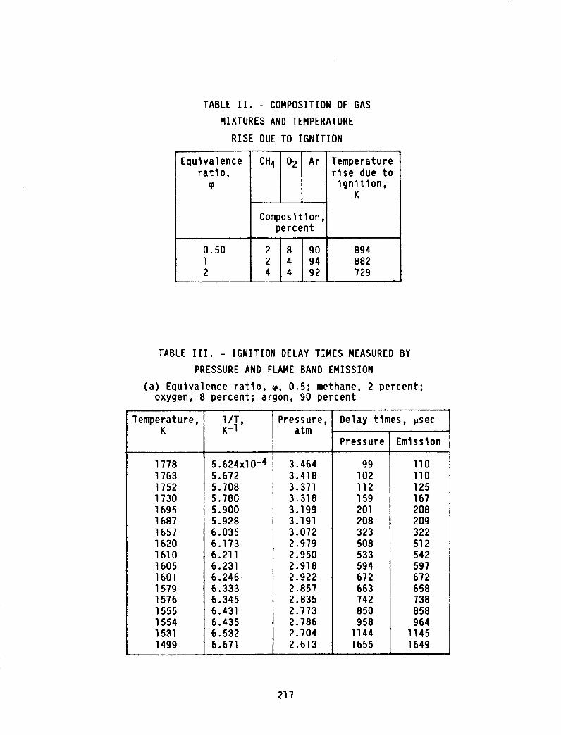
TABLEII. - COMPOSITIONOFGASMIXTURESANDTEMPERATURE
RISE DUETOIGNITION
Equivalenceratio,
CH4 02 Ar
Composition,percent
Temperaturerise due to
ignition,K
0.50 2 8 90 8941 2 4 94 8822 4 4 92 729
TABLE III.- IGNITION DELAY TIMES MEASURED BY
PRESSURE AND FLAME BAND EMISSION
(a) Equivalence ratio, _, 0.5; methane, 2 percent;oxygen, B percent; argon, 90 percent
Temperature,K
1778
1763
17521730
1695
1687
1657
1620
1610
1605
1601
1579
1576
1555
1554
1531
1499
l/T,K-1
Pressure, Delay times, usec
5.624xi0-4
5.672
5.708
5.780
5.900
5.928
6.035
6.173
6.211
6.231
6.246
6.333
6.345
6.431
6.435
6.532
6.671
atm
Pressure
3.464
3.418
3.371
3.318
3.199
3.1913.072
2.979
2.9502.918
2.922
2.8572.8352.7732.7862.7042.613
99
102
I12
159
201
208
323
508
533
594
672
663742
850
958I144
1655
Emission
II0
II0
125
167
208
209
322
512
542
597
672
658
738
858
964
I145
1649
217

IABLE III. Concluded.
(b) Equivalence ratio, m, l.O; methane,
oxygen, 4 percent; argon, 90 percent
2 percent;
Temperature,K
1915
18661802
1780
I/l,K-l
Pressure,atm
Delay
Pressu
1775174617321725171017071689168916551645163516291615
1593
5.222xi0 -4
5.3595.549
5.618
3.6803.536
3.354
3.279
5784
171201
5.638
5.727
5.774
5.797
5.848
5.858
5.921
5.921
6.042
6.079
6.116
6.139
6.192
6.2?8
.
3.
3.
3.
3.
3.
3.
278 185
183 295
147 383
122 397
082 427
077 531
023 525
3.032 589
2.932 794
2.900 867
2.876 967
2.855 1072
2.822 1163
2.761 1448
59
78
166
219
192
295
383
396
414
559
522
589
775
861
973
I075
I144
1471
times, usec
re Emisslon
(c) Mixture ratio, m, 2.0; methane, 4 percent;oxygen, 4 percent; argon, 92 percent
lemperature,K
1922
18561789
1770
1763
1730
17151712
i69i
1681
1677
1650
1627
1621
1602
5.203xi0 -4
5.388
5.590
5.650
5.6?2
5.7805.831
5.841
5.9i4
5.949
5.963
6.061
6.146
6.169
6.242
Pressure,arm
4.0123.797
3.583
3.524
3.485
3.381
3.3513.326
3.26U3.2283.217
3.134
3.063
3.043
2.984
Delay times, _sec
Pressure
67
116
198
249
318369
509
489
690
765
795
II02
1214
1319
1534
Emission
62
II0
201
271304
368
501
486
682
767
797
1096
1221
1321
1557
218

POGR QUALITY
Figure I. - Shock velocity measurement. Output from thin-film probeamplifier fed to digital oscilloscope. Time per point, 200 n sec. Lowertrace shows expansion of scale, which is helpful in determining exactti me shock wave passedprobe position.
219
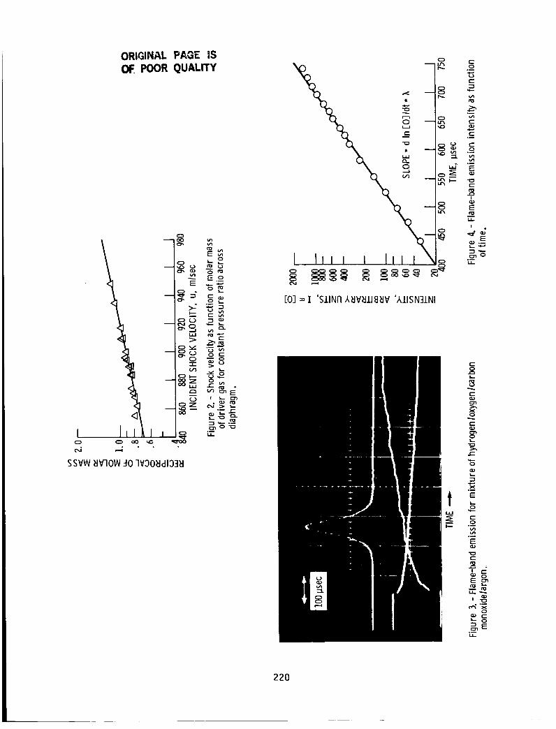
ORIGINAL PAGE iS
OE POOR QUALITY
IO
03
<3
O oO
¢1D
E_
--_o-S
0 r"
__. -
SSVW _IV-IOW.-I0 lV30_Id133_l
! l,,-
°_I.I-
0
[03:oI 'SIlNN,_IV_IlI]_IV '},llSN31NI
t,,J
,t-O
o=
=o
! •
RI,,,.
IB..,.,.
XO.,..,..
t'--
.,.C:
$..
.x_E
._o
EE(D
(,--
O
O
220
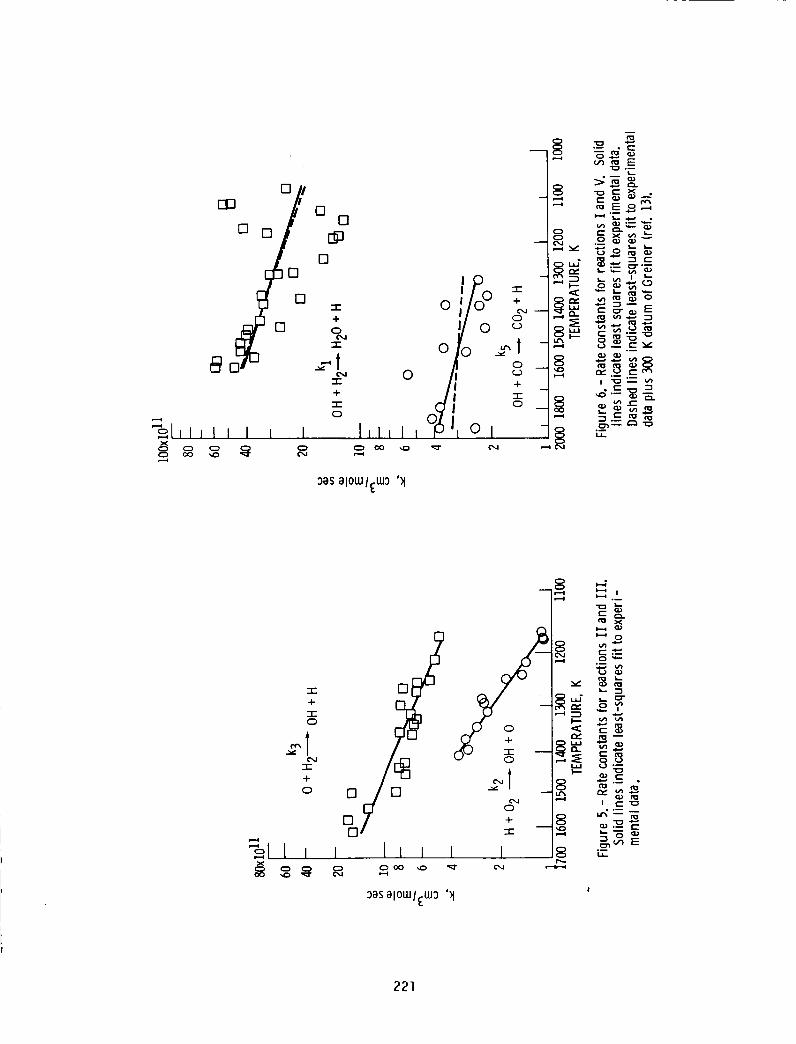
.=- -"13 °--
:)as alOWI£LU:) bt
.4--r0
_11 i I IL i I
:)as alOWl£W:) '3t
7
r- .
0 , ,--
+ _ _--'_-- _E
I 8 ,r
221

ORIGINAL PAGE _S
OF POOR QUALITY
!PRESSURE
Figure 7. - Delaytimes measuredat two locations in shock tube. Probes I and 2 are 7 and 83 mmfromreflectingsurface, respectively. P2is incident shock pressureand P5is reflectedshockpressure.Measureddelaytimeswere 712and 574psec.
222
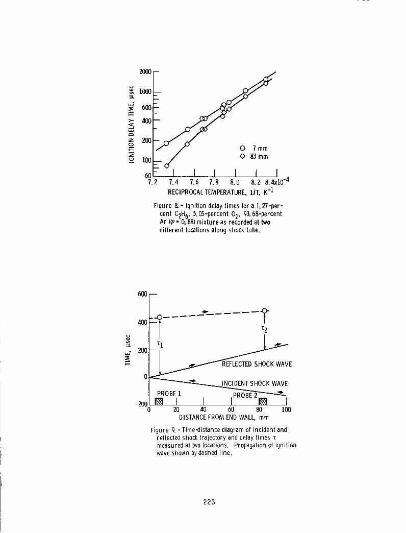
j200F,,,,_ _ 0 ?mm
_/ <> 83mm160[._00I I I I I I1.2 7.4 1.6 7.8 8.0 8.2 8.4xi0-4
RECIPROCALTEMPERATURE, lIT,K"I
Figure8.- Ignitiondelaytimesfora 1.2Y-per-
centC2H6,5.05-percent02,93.68-percentAr (_p-O.88)mixtureas recordedattwo
differentlocationsalongshocktube.
400
U
600--
--I
ua"
...... T2
200-rl
0 _CK WAVE
INCIDENTSHOCK WAVE
PROBE i PROBE 2-""_-_--I-2o0_ I I I0 20 40 60 80 100
DISTANCEFROM END WALL, mm
Figure9.-Time-distancediagramofincidentandreflectedshocktrajectoryanddelaytimesTmeasuredattwolocations.Propagationofignition
waveshown bydashedline.
223

2.40
Q,," 1.8W
u_ 1.21.1.1
o_el.
.6
o._k o
__ %_ rl
-_-o--0--_:13---o
DISTANCEFROMENDWALL,
mm
837
I I I I I2OOO0 400 800 1200 1600
DELAYTIMEAT PROBE1, lasec
Figure 10.- Ratio of ignition pressure to reflectedshockpressure, demonstratingenhanced igni-tion at secondprobeposition, particularly forshorter delaytimes.
r,,..
d
i-,
104
F
103
(#:1.0;AE: 246kj (.58.8 kcal)
(#:0.5;AE : 217kJ(51.9kcal)[] _ :2.0;AE : 246kJ(5&7kcal)
1o2 I I I I5. 5.6 6. 0 6. 4 6. 8xlO-4
DI_("IDDN/"AI TC^,'IDCDAT DC 1 IT K-tI'1,1,-_1_|1 i_'_,J_nl,. /LITII Ll'_n I Ul_.k, .ILl I,
Figure 11.- ._pO.l as function of lIT for all three
CH4mixtures, (#-0.5, 9" LO, and {#-2;0.
224
I.Report No.
NASA CP-2433
4. Title and Subtitle
Combustion Fundamentals
2. Government Accession No.
NASA Chlnese Aeronautical Establishment (CAE)
Symposium
7. Author(s)
9. Performing Organization Name and Address
National Aeronautics and Space AdministrationLewis Research Center
Cleveland, Ohio 44135
12. Sponsoring Agency Name and Address
National Aeronautics and Space AdministrationWashington, D.C. 20546
3. Recipient's Catalog No.
5. Report Date
6. Performing Organization Code
505-62-21
8. Performing Organization Report No.
E-3033
10. Work Unit No.
11. Contract or Grant No.
13. Type of Report and Period Covered
Conference Publication
14. Sponsoring Agency Code
15. Supplementary Notes
16. Abstract
A NASA - Chinese Aeronautical Establishment (CAE) symposium on combustion funda-
mentals was held at the NASA Lewis Research Center from September 23 - 27, 1985.This symposium was the result of an agreement (signed on 3anuary 31, 1979)
between the United States of America and the People's Republic of China on
cooperation in science and technology. A protocol agreement between NASA and CAE
was established in May 1983 to conduct exchanges and collaborative activities on
the basis of equality, reciprocity, and mutual benefit. The initial agreement
was to hold two symposia in the subject areas of structural analysis methods and
theoretical and experimental research in combustion fundamentals. Thls publica-
tion Is a compilation of the technical papers presented at the second symposium.It consists of five papers from senior specialists of CAE and seven papers from
NASA senior specialists.
17. Key Words (Suggested by Author(s))
Combustion; Fluid mechanics;Kinetics; Fuel sprays
18. Distribution Statement
Unclassified - unlimitedSTAR Category 7
19. Security Classif. (of this report)
Unclassified
20. Security Classif. (of this page)
Unclassified
21. No. of pages 22. Price*
231 All
*For sale by the National Technical Information Service, Springfield, Virginia 22161
"_" U. S. GOVERNMENTPRINTINGOFEICE:1987/748-120/40411