1

Combining Vehicle Routing and

Packing for Optimal Delivery

Schedules of Water Tanks

Jacob Stolka,c, Isaac Manna,d, Arvind Mohaisa,e, Zbigniew Michalewiczb,a,f

a) SolveIT Software Pty Ltd, Level 1, 99 Frome Street, Adelaide, SA 5000, Australia.

b) School of Computer Science, University of Adelaide, Adelaide, SA 5005, Australia; also at the

Institute of Computer Science, Polish Academy of Sciences, ul. Jana Kazimierza 5, 01-248 Warsaw,

Poland. Polish-Japanese Institute of Information Technology, ul. Koszykowa 86, 02-008 Warsaw,

Poland.

c)

Email: js@solveitsoftware.com (corresponding author).

d) Email:

im@solveitsoftware.com.

e) Email:

am@solveitsoftware.com.

f) Email:

zbyszek@cs.adelaide.edu.au.

Accepted on 31st January 2013 for publication in OR Insight

2

Abstract

This article describes a decision-support system that was developed in 2011 and is currently

in production use. The purpose of the system is to assist planners in constructing delivery

schedules of water tanks to often remote areas in Australia. A delivery schedule consists of

a number of delivery trips by trucks. An optimal delivery schedule minimises cost to deliver a

given total sales value of delivered products. To construct an optimal delivery schedule,

trucks need to be optimally packed with water tanks and accessories to be delivered to a set

of delivery locations. This packing problem, which involves many packing and loading

constraints, is intertwined with the transport problem of minimising distance travelled by

road.

Such a decision-support system that optimises multi-component operational problems is of

great importance for an organisation; it supports what-if analysis for operational and strategic

decisions and trade-off analysis to handle multi-objective optimisation problems; it is capable

of handling and analysing variances; it is easy to modify – constraints, business rules, and

various assumptions can be re-configured by a client. Construction of such decision-support

systems require the use of heuristic methods rather than linear/integer programming.

Keywords

Optimisation, clustering, vehicle routing, packing, shortest path.

Impact Statement

The original system described in this article shows new possibilities of hybridising and

adapting algorithms from various areas to solve real world problems, by:

addressing optimisation problems in the context of operations of a commercial

company;

solving these optimisation problems by combining and adapting various algorithms

from fields of data clustering, geographic information systems, shortest path finding,

vehicle routing, as well as packing and cutting.

3

1 Introduction

Large-scale business decision problems consist of interconnected components, but need to

be solved to achieve optimal results for a business as a whole. Even if we know exact

algorithms for solving sub-problems, it remains an open question how to integrate these

partial solutions to obtain a global optimum for the whole problem. Businesses need global

solutions for their operations, not partial solutions. This was recognised over 30 years ago in

the Operations Research (OR) community, when Russell Ackoff wrote: “… problems are

abstracted from systems of problems, messes. Messes require holistic treatment. They

cannot be treated effectively by decomposing them analytically into separate problems to

which optimal solutions are sought” (Ackoff, 1979). These remarks are directly applicable to

planning of optimal delivery schedules, for which intertwined routing, packing and

assignment problems need to be solved, that should not be considered in isolation.

Every time we solve a problem we must realise that we are in reality only finding the solution

to a model of the problem. All models are a simplification of the real world – otherwise they

would be as complex and unwieldy as the natural setting itself. Thus the process of problem

solving consists of two steps: (1) creating a model of the problem, and (2) using that model

to generate a solution (Michalewicz and Fogel, 2004):

Problem → Model → Solution

Also, a solution is only a solution in terms of a model of the problem. In solving real-world

problems there are at least two ways to proceed:

1. simplify the model so that exact methods might return better answers - in this case

the optimum solution to the simplified model does not correspond to the optimum

solution of the problem;

2. keep the model with all its complexities and use approximate, heuristic methods to

find a near-optimum solution – the more complexity there is in the problem (e.g. size

of the search space, conflicting objectives, noise, constraints), the more appropriate it

is to use a heuristic method

The system described in this article embodies a model of a delivery schedule planning

problem that is as accurate as possible. It combines various algorithms and heuristics to find

approximate solutions for a complex real-world business problem and is currently in

production use. The purpose of the system is to assist planners in constructing delivery

schedules of water tanks to often remote areas in Australia. A delivery schedule consists of

a number of delivery trips by trucks. An optimal delivery schedule minimises cost to deliver a

given value. To construct an optimal delivery schedule, trucks need to be optimally packed

with water tanks and accessories to be delivered to a set of delivery locations. This packing

problem, which involves many packing and loading constraints, is intertwined with the

transport problem of minimising distance travelled by road.

The rest of the article is organised as follows. Section 2 explains the business problem of

water tank delivery, its objectives, constraints, business rules and challenges, and puts it in

the context of related problems described in the literature. In Section 3 we describe

algorithms used to address the problem and their implementation in a production software

system. We discuss typical optimisation results generated by the system in Section 4.

Section 5 concludes the article.

4

2 The water tank transport and packing problem

An Australian company produces, sells and delivers rain water tanks. These products with a

large volume should be delivered to geographically dispersed customers, so transport cost is

high and transport cost minimisation an important competitive advantage. The transport cost

is considered with respect to the value of products delivered during the trips composing a

delivery schedule, so the packing component is very important to maximise delivered value

for a given transport cost.

The company’s delivery schedule planners need to make decisions involving numerous

variables related to production, intermediate storage, packing, transport and delivery of over

3000 products, divided in over 100 categories with different dimensions of rain water tanks

and accessories, to fulfil on the order of 1000 to 2000 customer orders per month, while

respecting numerous business rules and constraints that impact distribution decisions.

Orders come in continuously, so today’s optimal solution is not necessarily still optimal

tomorrow and re-optimisation is frequently necessary. Decisions to be made in this complex

logistics operation include:

the choice of one of several production facilities (plants) to make each product to be

delivered and dozens of storage facilities (agent sites, hubs, unbundling locations)

from which products in stock can be shipped,

selection of trucks for delivery trips from several types of trucks in a fleet of some 50

trucks, with or without trailers, to transport the goods, taking into account constraints

such as truck availability at each production facility, truck and trailer dimensions plus

the fact that only some truck/trailer combinations can transport the largest tanks;

because of considerable heterogeneity in product shapes and dimensions, truck and

trailer capacities cannot not be simple related to numbers of products transported,

but are expressed as total length, width, height, and weight of a load, in addition to

other considerations such as possible overhang, etc.

packing of goods on trucks and trailers in an optimal way, taking into account

numerous constraints related to truck, trailer and product dimensions, as well as

several ways to bundle, pack and stack products according to product type;

selection of drivers from over 100 possible drivers, taking into account their

availability, including timetables, maximum hours of work, availability for making

longer trips, qualifications (not all drivers can drive all trucks or transport all tanks);

selection of optimal routes to travel in order to minimise transport cost relative to

delivered sales value.

All these decisions need to be made to minimise the key performance indicator of transport

cost as percentage of delivered sales value.

Each of the above problems is hard to solve in isolation. For example, the problem of

packing of goods on trucks and trailers is impossible to solve with standard 2D or 3D

packing algorithms, as different types of tanks can be packed in different ways, e.g. bundled

inside each other, on top of each other, taking into account various constraints, in a pyramid

stacking configuration, or as loose items.

5

Further, the problems are connected, as decisions made for one problem may impact

decisions for another problem. The ‘optimal’ decision for one problem may prevent finding

the overall optimal solution. Thus, packing and routing problems are intertwined, as the

destination locations of items packed on a truck/trailer for a trip determine the final delivery

destinations to be visited. Water tanks can often be bundled inside each other, making

possible efficient packing of a truck and/or trailer, but they can be unbundled only at specific

agent locations of the company, which has to be done prior to final delivery to customer

locations – so there is a trade-off between efficient packing and the need to travel a longer

distance to visit unbundling sites in addition to final delivery sites. Or a decision of using a

particular truck with a trailer for a trip may prevent another delivery which requires a driver

with appropriate qualifications. In general, the decision to pack a tank on a truck for a

particular delivery trip always needs to take into consideration the implications for the routing

of that trip. Adding a tank can increase delivered value, but also transport cost due to

increased distance to travel. It may well be advantageous to add the tank to a different trip

that already goes near the delivery location of the tank, even if that leaves the first trip less

than optimally packed.

The overall water tank delivery problem has some similarities with other well-known

optimisation problems described in the literature, reviewed in subsections 2.1 – 2.3, but also

has peculiar features which are not found elsewhere. We have developed algorithms to

solve the problem by adapting and combining selected optimisation algorithms for problems

with similar characteristics.

2.1 Travelling salesman problem

The travelling salesman problem (TSP) is the problem of finding the shortest tour through a

set of a positive integer number of N locations so that each location is visited exactly once

and the tour returns to its starting point (Potvin, 1996; Applegate et al, 2006). Like the TSP,

the water tank delivery problem involves visiting a given set of locations while travelling the

shortest possible distance. In particular, from a hub several trips are made, which can each

be regarded as a separate TSP. However, trips need to satisfy numerous constraints related

to various ways of loading products to be delivered on trucks and/or trailers with different

capacities, as well as assigning drivers with different qualifications and working hours to

trips. Therefore standard TSP algorithms are not suitable for the water tank delivery

problem.

2.2 Vehicle routing problems

A vehicle routing problem (VRP) consists of determining a set of vehicle trips from a depot to

customers, of minimum total cost, such that each trip starts and ends at the depot, each

client is visited exactly once, and the total demand handled by any vehicle does not exceed

the vehicle capacity (Clarke and Wright, 1964; Prins, 2004; Cordeau et al, 2007a; Perboli et

al, 2008). Variants of the VRP that have been studied include:

the classical vehicle routing problem: a commodity is to be delivered at minimal cost

from a depot to a set of customers, given a nonnegative demand for each customer,

travel costs for each route, and a fixed capacity for each vehicle of a fleet of identical

vehicles; in the water tank delivery problem capacity and bundling requirements

determine constraints on the number and type of tanks that can be loaded on a truck

6

- in existing VRP algorithms truck capacity is taken into account, but bundling of

tanks introduces special constraints on the numbers of tanks of each type and size

that can be loaded on a truck;

VRPs with loading constraints, reviewed in (Iori and Martello, 2010): loading

constraints that have been analysed include two and three-dimensional loading

constraints, as well as some special variants such as multi-pile loading, taking into

account order of loading, etc.; again, the water tank delivery problem has special

characteristics that have not been studied anywhere else, to our knowledge, such as

the possibility of bundling and the necessity of visiting special intermediate locations

where unbundling can take place;

the vehicle routing problem with time windows is a generalization of the classical

VRP in which service at every customer must start within a given time window;

the inventory routing problem is an extension of the VRP which integrates routing

decisions with inventory control;

stochastic vehicle routing problems are extensions of the deterministic VRP in which

some components are random;

a multi-depot VRP: delivery trips take place to several delivery regions, each with a

hub where unbundling is done; the water tank delivery problem is a multi-depot VRP;

in the multi-depot VRP described in (Ho et al, 2008) it is assumed that each depot

has enough stock to supply the demand of all customers; for the water tank delivery

problem we could assume that a depot stock is the load of truck brought from the

factory plus consignment stock present at the sales agent’s site; however, we should

also optimise allocation of trucks to sales agents; further, deliveries can be made not

only from hubs, but also on the way back from a hub to the factory; tanks can be

loaded at the factory, but also from consignment stock at the hubs;

pickup and delivery problems: VRPs where a set of transportation requests is

satisfied by a given fleet of vehicles (Cordeau et al, 2007b); each request is

characterised by its pickup location (origin), its delivery location (destination) and the

size of the load that has to be transported from the origin to the destination; in the

variant with time windows, for each pickup and delivery location, a time window and

loading and unloading times are specified; the load capacity, the maximum length of

its operating interval, a start location and an end location are given for each vehicle;

in order to fulfil the requests, a set of routes has to be planned such that each

request is transported from its origin to its destination by exactly one vehicle

(Pankratz, 2005); a variant with separate pickup and delivery tours and goods to be

stacked in a container on a truck is described in (Petersen et al, 2010); in another

variant intermediate storage facilities are used (Angelelli and Speranza, 2002).

For the water tank delivery problem an important limitation of the formulation of VRPs is the

assumption that only one commodity is transported and both vehicle capacities and

customer demand are expressed as quantities of this single commodity, while water tanks

have many different sizes and shapes, trucks (with or without trailers) have different

dimensions and drivers have different qualifications for driving trucks and transporting tanks

depending on dimensions; thus the possibility of transporting a given load of tanks is

determined by all these variables rather than a simple capacity expressed as a single

number.

7

2.3 Cutting and packing problems

In cutting and packing problems a set of large objects and a set of small items are given.

The problem is to select some or all small items, group them into one or more subsets and

assign each of the resulting subsets to one of the large objects such that the small items of

the subset lie entirely within the large object and do not overlap, and a given objective

function is optimised (Wäscher et al, 2007). According to the typology developed by

Wäscher et al (2007), who provide detailed references for the different types of problems,

cutting and packing problems can be categorised in the following types:

output maximisation: a (sub)set of small items of maximal value has to be assigned

to all of a given set of large objects:

o identical small items: Identical Item Packing Problem;

o weakly heterogeneous small items: Placement Problem;

o strongly heterogeneous small items: Knapsack Problem;

input minimisation: all small items are to be assigned to a subset of the large objects

of minimal ‘‘value’’:

o arbitrary small items: Open Dimension Problem;

o weakly heterogeneous small items: Cutting Stock Problem;

o strongly heterogeneous small items: Bin Packing Problem.

The water tank delivery problem is an input minimisation problem, as all tanks have to be

delivered at minimal cost. Water tanks can be grouped into relatively few groups of products

with identical shape and size, so problem of packing a set of water tanks on available trucks

is a Cutting Stock Problem.

However, the delivery cost depends on the route to be travelled by the truck on which the

items are packed which in turn is not independent of items packed on and routes to be

travelled by other trucks.

3 The water tank transport and packing optimiser

We have combined several algorithms in a decision support system to assist planners to

make numerous packing and routing decisions for the construction of near-optimal delivery

schedules of water tanks and accessories on an on-going basis. We have made use of

these algorithms to construct heuristics for finding delivery schedules with desirable

characteristics, as detailed below.

The system generates a delivery schedule using the following steps, which are detailed in

the corresponding subsections of this section.

1. Basic data are loaded including product data, transport data, driver data, production

and storage sites from which delivery trips depart, sales agent sites that can be used

for unbundling and intermediate storage, and geographical coordinates

corresponding to all agent and delivery location addresses.

8

2. Periodically new data are loaded on orders of water tanks and accessories and on

updated stock levels.

3. Road distances are calculated to be used for clustering of locations and for detailed

routing of trips.

4. All agent and customer locations to be visited are clustered using a clustering

algorithm.

5. Each cluster is processed to construct delivery trips.

6. When attempting to add products to each trip, constraints are checked related to

product and transport dimensions and weight, as well as various packing

possibilities.

7. After determining the load of each trip, the best unbundling site is chosen, i.e. the

unbundling site that makes possible the shortest possible distance to be travelled by

the trip.

8. The best set of delivery trips is retained as recommended delivery schedule.

In the remaining sections the term “items” is the overarching term referring to round,

rectangular and odd-shaped products that need their dimensions to be considered when

placing them on a delivery trip. The term “tanks” refers to round items (literally tanks), and

“transport” is the abstracted concept of trucks and trailers. A “transport tray” is the space

available to place items.

3.1 Basic data

To take into account packing and loading of products on trucks and trailers, data are loaded

on product dimensions, as well as truck and trailer dimensions and carrying capacity.

Products are organised in groups of products with the same shape (round or rectangular),

weight, height, width, depth, bundling diameter (the dimension considered for bundling), and

stacking/packing options. Trucks and trailers are organised in transport models which define

their dimensions and loading capacity, including height, width, length, possible overhang and

possible load weight.

Data on reselling agents include information on the possibility to use their site for unbundling

and the maximum bundle weight that can be handled, as well as address details and

geographical coordinates of the sites. We have used a geo-location service to obtain

geographical coordinates corresponding to delivery and agent addresses.

3.2 Periodic data

Periodically data on new orders are loaded into the system, including order date and due

date, customer information, type of order, and delivery address, with geographical

coordinates of the delivery site. Each order has one or more order items, with product,

product group, quantity and sales price information. The delivery schedule will be re-

optimised to accommodate delivery of these new orders.

9

Table 1. Water tank transport and packing algorithms

1) Delivery destinations and intermediary agent locations:

1.1) retrieve geolocations and road network data

1.2) calculate distances between locations to be visited with Dijkstra shortest path algorithm

2) Initial clustering:

2.1) cluster destination locations with FLAME clustering algorithm:

2.1.1) for each object (delivery location), find the k nearest neighbours, calculate their proximity, calculate object density and define the object type (CSO/outlier/other)

2.1.2) assign fuzzy membership by local approximation

2.1.3) construct clusters from the fuzzy memberships

2.2) post-process clusters to avoid clusters that are too large: a maximum cluster size is specified - if the largest distance between two locations in a cluster exceeds the maximum size, the cluster is split into two clusters by allocating each location in the cluster to a new cluster according to distance to each of the two locations with maximum distance

2.3) if desired, post-process clusters to avoid clusters that are too sparse: if the average distance between cluster locations is too large, split the cluster in two - users may prefer less than optimal trips that are not completely loaded but are confined to a relatively small region, rather than better loaded trips covering a larger region, when they expect the incompletely loaded trips to be filled with new orders to come in later

3) Construct trips: for each cluster, select a truck and a driver, then attempt to add items to be delivered to a trip in order of decreasing distance of delivery locations to the plant, checking if items can be bundled, packed or stacked:

3.1) select truck and driver

3.2) bundling: attempt to bundle an item, given constraints as described in section 3.6.1

3.3) packing and stacking: attempt to pack and/or stack an item, using a 2D column packing algorithm combined with stacking constraints, as described in section 3.6.2

4) Combine clusters of remaining destinations, if not all items have been assigned to trips in step 3) and if this is desired by the user; as in step 2.3, users may decide to skip this step for similar reasons: not recombining clusters will tend to produce less well loaded trips confined to smaller delivery regions

5) Iterate 3), in combination with 4) if desired, until all ordered products are assigned to trips

10

Table 1. Water tank transport and packing algorithms (continued)

6) For each trip, find the best unbundling location:

6.1) calculate maximum and minimum latitude and longitude for all delivery locations of the trip

6.2) for each possible unbundling location within the area contained in these bounds, construct trip routes with the algorithm described in step 7) – retain the unbundling location with the shortest trip distance

7) For each unbundling location, determine the best routing of ‘hub run’ trips from unbundling location to customers with a modified Clark & Wright algorithm:

7.1) initial solution: each vehicle serves exactly one customer

7.2) for each pair two distinct routes, compute possible savings by merging them, for example: merging routes servicing customers and leads to savings

; if , the merging operation is convenient

7.3) all saving values are stored in a half-square matrix

7.4) matrix is sorted in not-increasing order of the values to create a list of

saving objects composed by the triplets - the higher the saving value, the

more appealing the associated merge operation

7.5) the saving objects in list are now sequentially considered: if the associated merge operations are feasible, they are carried out, where merge feasibility is determined as follows:

7.5.1) overload of the vehicle: a merge operation is not feasible, if load to be transported violates vehicle capacity – in the original Clark & Wright algorithm vehicle capacity is a given quantity of goods; we have modifies this by a check if the goods can be packed on the truck, given the loading constraints

7.5.2) internal customers: a customer which is neither the first nor the last at a route cannot be involved in merge operations

7.5.3) customers both in the same route: if customers and suggested by saving are at extremes of the same route (first or last), the merge

operation cannot be performed (no sub-tours are allowed)

7.6) a solution is found, when no more merge operations are possible

11

3.3 Calculation of road distances

One desirable characteristic of a solution is that a scheduled delivery trip visits customer

locations (for delivery) and agent locations (for unbundling and/or delivery) that are relatively

close to each other. Therefore, it is useful to cluster locations to be visited. Clustering

algorithms (Xu, 2005) need a proximity measure as a basis for clustering. Once it is decided

that a trip is to visit a number of delivery locations, based on the results of the clustering

algorithm, the exact routing of the trip has to be determined by a vehicle routing algorithm. In

the case of the water tank transport problem, delivery cost is directly related to distance

travelled by road, so the obvious proximity measure to be used is distance by road.

This immediately leads us to the problem of determining distance by road between locations

to be visited. Data on the Australian road network have been obtained from Geoscience

Australia1. Now, to determine distances between any given pair of locations from the road

network data, geographical coordinates of these locations need to be known. Typically, in

the context of the business problem of water tank deliveries, only address data are given, so

a geolocation method is needed to determine geographical coordinates from address data.

Once geographical coordinates have been obtained, calculating the distance by road

between two locations can be done by determining the shortest path between these

locations in the graph defined by the road network.

A well-known algorithm to calculate the shortest path between nodes or vertices in a graph is

Dijkstra’s algorithm (Dijkstra, 1959; Shaffer, 2001: 377-381). We have made use of Dijkstra’s

algorithm to calculate road distances between locations to be visited by delivery trucks.

These distances are used for clustering of locations and, after trip construction, calculating

the shortest distance to be travelled.

3.4 Clustering of locations

Many clustering algorithms, such as k-means or fuzzy k-means, make assumptions about

the number of clusters to be generated. For the purpose of determining optimal delivery

trips, this is not desirable, as the set of locations to be visited perpetually changes according

to customer orders to be fulfilled and/or agent locations being activated or deactivated by the

water tank production company. Therefore, a clustering algorithm is needed that determines

an optimal clustering for any set of locations without assumptions about the number of

locations. Another desirable feature of a clustering algorithm is the possibility to fine-tune the

algorithm by setting parameters to be able to control, for example, the maximum size of

generated clusters, or the approximate number of locations in a cluster.

A clustering algorithm with such features is the fuzzy clustering by Local Approximation of

Membership (FLAME) algorithm (Fu and Medico, 2007), originally developed for

bioinformatics applications. FLAME clusters data objects through three main steps:

1. extraction of local structure information by calculating object density from the

distance/proximity between each object and its k-nearest neighbours; objects with

the highest density among their neighbours are identified as cluster supporting

1 Available from http://www.ga.gov.au.

12

objects (CSOs) and serve as prototypes for the clusters; outliers are also identified in

this step;

2. assignment of fuzzy membership by local approximation; initially each CSO defines a

cluster and is assigned with full membership to its cluster, while outlier objects are

assigned with full membership to the outlier group and all other objects are assigned

with equal membership to all clusters; then, an iterative process is performed to

approximate the fuzzy memberships of objects which are not CSOs or outliers, for

which the membership is fixed; at each iteration, the fuzzy membership of each

object is updated by a linear combination of the memberships of its nearest

neighbours, weighted by their proximity; in this process the fixed, full memberships of

CSOs and outliers exert an influence on the membership of their neighbours, which

subsequently propagates in the neighbourhood network during the following

iterations so that the final membership of each object (except CSOs and initial

outliers) is the result of the direct and indirect influence of the memberships of all

other objects;

3. construction of clusters from the fuzzy memberships, which can be made in two

ways: (i) by assigning each object to the cluster in which it has the highest

membership degree (one to one object-cluster relationship), or (ii) by applying a

threshold on the memberships, and assign each object to the one or more clusters in

which it has a membership degree higher than the threshold (one-to-many object-

cluster relationship).

3.5 Cluster processing to construct delivery trips

One of the results of processing a cluster of delivery locations is to find the nearest base

plant, which becomes the originating location for a trip. An example of clusters is shown in

Figure 1.

Trucks and drivers are selected on the basis of their home base plant, their availability within

the preferred scheduling period, the maximum tank sizes they can transport, and the drivers’

preferred trucks. The best driver and truck to use are decided on a “best fits” basis for the

provided list of items from the cluster. Each cluster of delivery locations is analysed, starting

with the items furthest from the departing plant for the trip. For each item the algorithm will

attempt to recreate the trip for each driver and truck, finding the best option for each

combination.

The process of adding one item to analyse at a time and rebuilding continues until:

1. there is only one trip – this will be able to take the highest number of items (and

implicitly the load will be worth the most) in the given period;

2. there are multiple trips that can carry all items in the cluster; the system will then

choose the truck/driver combination that can leave the soonest.

If there are no possible departures in the preferential departure period, the system will

consider all trucks and drivers, not just those available soonest, and repeat the above

selection process.

13

Figure 1. An example of clustered locations. The coloured dots represent delivery destinations,

with a different colour for each cluster (encircled) that has been found by the clustering algorithm.

Crosses represent agent sites that can be used for unbundling.

3.6 Trip construction by packing and bundling

Trips are constructed with two methods of placing items on the transport: bundling and

packing. Each method of placing items has its own rules. Both of these methods are subject

to the space available on a transport, which is affected by overhang rules. An example trip

loading is shown in Figure 2.

Overhang is the means of utilising the space between a truck and its attached trailer, if there

is a trailer: dimensions of transported items can, under certain conditions, be slightly larger

than truck or trailer dimensions. Items are placed, if possible, bundled, the most efficient way

of placing items, else packed. For each attempt to place each item on one of the transport

trays, the possible weight is considered, as both trucks and trailers have maximum weight

allowances.

14

Figure 2. A loaded trip. The top part of this screen is a graphical view of a truck and trailer load with

bundled and packed items, seen from the side and from above. The table at the bottom gives details

on the items loaded: if they are loaded on the truck or the trailer, if they are packed or bundled, as

well as product code, product group, shape, dimensions, weight and unbundling location.

3.6.1 Bundling

Bundling is a recursive method of cutting the top of the tank off, placing a smaller tank on the

inside, and then repeating the process. Bundling can only be performed at plants, and can

only be undone at specifically chosen sites that contain the equipment and expertise to

unbundle. Bundling rules are:

the width and length of an inner tank must be smaller than the width and length of the

enclosing outer tank;

the maximum straight-line distance of an inner tank’s shape must be less than the

diameter of the outer tank;

custom-built tanks (with special specifications requested by customers) and the

largest tanks cannot have their lids cut, so cannot be on the outside of a bundle, as

tanks can only be placed inside other tanks with cut lids;

other tanks that can have their lids cut are marked as such by a flag;

there are minimum and maximum differences in diameter that two tanks can have to

place one inside another;

some rectangular items can be bundled inside a tank, but a round item cannot be

bundled inside a rectangular item;

all tanks are placed across the transport tray on their sides, with the round

tops/bottoms facing outwards and the rounded single side lying on the tray;

bundling only considers the length of the tray.

15

As the bundling algorithm attempts to bundle each item, it checks the available space at the

front of the trailer, the remaining space of the trailer, and the available space on the truck, in

that order. For all truck/trailer combinations, the largest (or equal-largest) amount of space is

available at the front of the trailer, then on the rest of the trailer. The algorithm starts a new

bundle in available space, if possible. When adding a new tank, it also checks if it is possible

to fit it in an existing bundle.

Bundling also considers possible overhang of one item over another. For example: if a

50,000L tank and a 5,000L tank were placed side-by-side, the 5,000L tank would be able to

“tuck under” the larger tank by a margin significant enough to consider.

3.6.2 Packing and stacking

Packing is done by a custom packing algorithms: a 2D column packing algorithm, combined

with “stacking” (placing items of the same product group on top of each other) and/or

“pyramid stacking” (placing tanks of the same product group in a pyramid, e.g. 3 in the base

layer, 2 in the next layer, 1 in the top layer). Items are checked for merging possibilities with

stacking or pyramid stacking and placed into rectangular objects representing their final size;

these rectangles can then be packed.

If an item can be stacked, the stacking algorithm tests for any packed items existing on the

trip of the same product group, and whether there are less items stacked than the maximum

allowance. The algorithm will then merge the items into a new rectangle which will have the

same base size from a top-down view, and so doesn’t affect the 2D column packing.

Pyramid stacking is done via checking for the same items on the trip, placing them together

into a new rectangle based on the height limits (i.e. 2 or 3 rows high) and re-testing the 2D

column packing of the trip with this new rectangle.

The 2D column packing algorithm splits up items into rows across the width of the transport

tray by segregating all items into two lists: one of items with longest edge length more than

half the width of the transport tray, and another with items with longest edge length less than

half the width of the transport tray. The largest items are placed first, one per row, as two

cannot be fitted across in the same row. As each item is placed, a check is made if any of

the small items can be placed in the same row (to minimise usage of the length of the

transport tray).

3.7 Packing and routing of trips

Once the delivery locations of a trip have been determined, the shortest route for the trip has

to be calculated. A trip leaves a plant to visit its delivery locations and returns to the plant, or

first visits an unbundling location, unbundles its tanks and makes a number of smaller trips

(hub runs) to customer sites. A well-known algorithm to find an approximately shortest route

for a vehicle making deliveries from a central depot to a number of delivery points is the

algorithm formulated by Clarke and Wright (1964). The Clarke & Wright algorithm assumes a

fixed vehicle capacity. It starts with an initial solution where a vehicle serves exactly one

customer at a time and returns to the depot. It then calculates savings, in terms of distance

travelled, that can be obtained by merging two routes into one. Routes are merged, starting

with merges that lead to the highest savings, without violating the vehicle capacity constraint.

The process is repeated until no further savings are possible (Battarra et al, 2007).

16

Optimal routing and packing is decided via a modified Clark & Wright algorithm. Instead of a

fixed truck capacity, actual loading constraints are taken into account. The algorithm initially

splits all visiting drop-off points into separate tours from a central “unbundling” site (if the trip

has bundled items; if the trip only contains packed items, the departing plant is used) and

then decides whether to combine two tours based on the possible saved distance. An

example trip routing calculated by the algorithm is shown in Figure 3.

Figure 3. A trip routing. This trip leaves the central plant at Lonsdale and first goes to an agent site

in Maitland, where unbundling is done. From the unbundling site hub run trips are made to the

delivery locations. Hub run trips return to the unbundling location to pick up items for the next hub run,

except the last hub run trip, which goes back to the plant. Locations of this trip are numbered from 1

to 20 in order of visit. Routes are shown as straight lines for rendering performance reasons only.

Actual distances travelled and used by the algorithms are distances by road.

This algorithm will:

use a central departure point (“centre”):

o the “unbundling” site if the trip contains bundled items;

o the departing plant if the trip only contains packed items;

split all locations to visit into separate “site” objects;

create “route” objects for every site object to link to, so that every site knows what

route is taken to reach it:

o initially these routes are from the centre to the site and back to the centre;

o routes contain a sequential list of visited sites;

17

for every site, find the possible saving that could be obtained by merging with every

other site, i.e. the distance that would be saved from having to travel without merging

the routes, possibly taking into account the constraint that items from the same order

have to be delivered together;

sort this list of savings in order of the items that would save the most;

for every saving, check whether the routes can be merged:

o the sites must be on different routes;

o the transport must be able to pack the items (no unbundling is possible) using

the packing algorithm described in Section 3.6;

o the sites must be either the first or last site in their route list;

this stage is continued until all possible savings have been assessed, and a set of

tours from the centre can be created from the routes; note:

o bundled trips may have more than one tour;

o packed trips will only have one tour;

a final improvement is made, as the last hub run trip does not need to return to the

unbundling location, but can return directly to the plant, dropping off its items en

route; the algorithm determines for which one of the hub run trips this is the most

advantageous.

3.8 Delivery schedule

The system was delivered and integrated with the company’s databases, and it is in daily

use by planners. Basic data on products, trucks and trailers, drivers, production and storage

sites, and sales agent sites, as well as periodic updates of orders and stocks, are imported

from the company’s main transactions database system.

A recommended delivery schedule is produced by the packing and transport optimisation

system. An example is shown in Figure 4. The delivery schedule, including details of orders

and products loaded on trips and exacts routes of trips, is submitted to approval by a

planner. After approval the schedule is exported to the company’s database system in view

of order processing, production planning, etc.

4 Results

The water tank packing and transport optimiser produces delivery schedules as for example

shown in Figure 4. The optimiser is used in production by the delivery trip planners of the

company it was built for. Key benefits obtained are:

more profitable trips as the optimiser locates optimal opportunities to maximise trip

loads and minimise transport cost;

fewer trips cancelled owing to trips not passing verifier criteria – fewer dissatisfied

customers (end users and resellers) and improved service levels;

more proactive order fulfilment, with reduced delivery times after order placement;

reduced routine work for planning delivery schedules, so more time is available for

customer service and sales work, resulting in improved customer relationship

management;

18

removal of duplication of information, voluminous paperwork, copying and storage of

hard copies; reduction of carbon footprint across the business;

greater visibility of the planning process and a single point of reference for

information;

more flexible automated reporting for management.

Figure 4. A delivery schedule generated by the optimiser. In the top panel a line view is shown of

the timing of constructed delivery trips, ordered by the trucks used for the trips. In the bottom left table

one trip is selected, with information on truck, trailer and driver used, number of items packed on the

trip, departure and arrival date, freight cost as percentage of sales value and status. The bottom right

tables give details of the items loaded on the trip.

Delivery schedule planning is an on-going process, with new orders constantly coming in,

while a delivery schedule produced by the optimiser is based on a snapshot of orders at a

specific point in time. Therefore, actually executed delivery trips typically are a subset of the

solution produced by the optimiser. Relatively disadvantageous trips in the solution are not

approved, but remain in the system as draft trips. When new orders have come in, the

optimiser is rerun and items on draft trips are combined with new order items to create new

trips. Due to this process, it is not possible to compare optimiser results and manual results

19

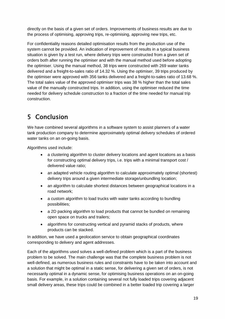
directly on the basis of a given set of orders. Improvements of business results are due to

the process of optimising, approving trips, re-optimising, approving new trips, etc.

For confidentiality reasons detailed optimisation results from the production use of the

system cannot be provided. An indication of improvement of results in a typical business

situation is given by a test run, where delivery trips were constructed from a given set of

orders both after running the optimiser and with the manual method used before adopting

the optimiser. Using the manual method, 38 trips were constructed with 269 water tanks

delivered and a freight-to-sales ratio of 14.32 %. Using the optimiser, 39 trips produced by

the optimiser were approved with 356 tanks delivered and a freight-to-sales ratio of 13.68 %.

The total sales value of the approved optimiser trips was 38 % higher than the total sales

value of the manually constructed trips. In addition, using the optimiser reduced the time

needed for delivery schedule construction to a fraction of the time needed for manual trip

construction.

5 Conclusion

We have combined several algorithms in a software system to assist planners of a water

tank production company to determine approximately optimal delivery schedules of ordered

water tanks on an on-going basis.

Algorithms used include:

a clustering algorithm to cluster delivery locations and agent locations as a basis

for constructing optimal delivery trips, i.e. trips with a minimal transport cost /

delivered value ratio;

an adapted vehicle routing algorithm to calculate approximately optimal (shortest)

delivery trips around a given intermediate storage/unbundling location;

an algorithm to calculate shortest distances between geographical locations in a

road network;

a custom algorithm to load trucks with water tanks according to bundling

possibilities;

a 2D packing algorithm to load products that cannot be bundled on remaining

open space on trucks and trailers;

algorithms for constructing vertical and pyramid stacks of products, where

products can be stacked.

In addition, we have used a geolocation service to obtain geographical coordinates

corresponding to delivery and agent addresses.

Each of the algorithms used solves a well-defined problem which is a part of the business

problem to be solved. The main challenge was that the complete business problem is not

well-defined, as numerous business rules and constraints have to be taken into account and

a solution that might be optimal in a static sense, for delivering a given set of orders, is not

necessarily optimal in a dynamic sense, for optimising business operations on an on-going

basis. For example, in a solution containing several not fully loaded trips covering adjacent

small delivery areas, these trips could be combined in a better loaded trip covering a larger

20

area. However, trips covering a too large area were considered undesirable and it was

preferred to keep the sub-optimal smaller trips and postponing their departure until more

orders came in. Thus, one important lesson learned is the fact that optimal delivery

schedules for a business are delivery schedules that make sense to business planners.

To obtain good solutions, not only does each of the algorithms used need to perform well,

but their partial results need to be combined to produce acceptable overall solutions. For

example, the initial clustering of delivery locations is not necessarily optimal, as it does not

consider truck and driver selection or loading constraints. We have taken this into account

using an iterative approach, re-clustering remaining delivery destinations when all initial

destinations in a cluster cannot be served by a constructed trip. We have chosen a

clustering algorithm which does not make assumptions about the number of clusters to be

generated and is efficient.

Similarly, once deliveries are assigned to a trip, the optimal route of the trip is determined by

evaluating routes for a set of possible unbundling locations. This involves numerous

executions of the shortest route algorithm. For this reason we have adapted the Clark &

Wright algorithm, which gives only approximate solutions, but is very efficient.

One of the main performance bottlenecks encountered was the calculation of road distances

from data on the Australian road network, because actual road distances between a many

locations are required. The road network is represented as a graph with nodes at numerous

intermediate locations, in which, in the worst case, shortest paths have to be found between

all possible locations that could be visited.

Possible improvements of the system that could be envisaged include:

performance improvements of road distance calculations by applying simple

heuristics to eliminate calculation of distances between locations that are unlikely to

be used;

using an evolutionary algorithm to explore alternative solutions, for example mutating

existing solutions by exchanging deliveries between trips in the solution.

Acknowledgements

The authors express their gratefulness to the following persons who have contributed to the

development of the software described in this article: software developers Jingjing Dong,

Alexis Pflaum and Ayaz Hassan; business analysts Josh Boston and Daniel Spitty; scientist

Mohammadreza Bonyadi, various testers at SolveIT Software.

References

Ackoff R (1979). The future of operational research is past. Journal of the Operational

Research Society 30(2): 93-104.

Angelelli E and Speranza M G (2002). The periodic vehicle routing problem with

intermediate facilities. European Journal of Operational Research 137(2): 233-247.

21

Applegate D L, Bixby R.E., Chvátal V and Cook W J (2006). The Traveling Salesman

Problem: A Computational Study. Princeton University Press: Princeton.

Battarra M, Baldacci R and Vigo D (2007). Clarke and Wright algorithm. Presentation

retrieved from http://www.scribd.com/doc/35387231/Clarke-Wright on 19/01/2012.

Clarke G and Wright J W (1964). Scheduling of vehicles from a central depot to a number of

delivery points. Operations Research 12(4): 568-581.

Cordeau J-F, Laporte G, Potvin J-Y and Savelsbergh M W P (2007b). Transportation on

demand. In: Barnhart C and Laporte G (eds). Transportation, Handbooks in Operations

Research and Management Science 14: 429–466. Elsevier, Amsterdam.

Cordeau J-F, Laporte G, Savelsbergh M W P and Vigo D (2007a). Vehicle routing. In:

Barnhart C and Laporte G (eds). Transportation, Handbooks in Operations Research and

Management Science 14: 367–428. Elsevier, Amsterdam.

Dijkstra E W (1959). A note on two problems in connexion with graphs. Numerische

Mathematik 1: 269–271

Fu L and Medico E (2007). FLAME, a novel fuzzy clustering method for the analysis of DNA

microarray data. BMC Bioinformatics 8(3): http://www.biomedcentral.com/1471-2105/8/3.

Ho W, Ho G T S, Ji P and Lau H C W (2008). A hybrid genetic algorithm for the multi-depot

vehicle routing problem. Engineering Applications of Artificial Intelligence 21(4): 548-557.

Iori M and Martello S (2010). Routing problems with loading constraints. Top 18: 4-27.

Michalewicz Z and Fogel D B (2004). How to Solve It: Modern Heuristics, 2nd edition.

Springer-Verlag: Berlin, Heidelberg.

Pankratz G (2005). A grouping genetic algorithm for the pickup and delivery problem with

time windows. OR Spectrum 27(1): 21-41.

Perboli G, Pezzella F and Tadei R (2008). EVE-OPT: a hybrid algorithm for the capacitated

vehicle routing problem. Mathematical Methods of Operations Research 68(2): 361-382.

Petersen H L, Archetti C and Speranza M G (2010). Exact solutions to the double travelling

salesman problem with multiple stacks. Networks 56(4): 229-243.

Potvin J-Y (1996). Genetic algorithms for the traveling salesman problem. Annals of

Operations Research 63(3): 337-370.

Prins C (2004). A simple and effective evolutionary algorithm for the vehicle routing problem.

Computers & Operations Research 31(12): 1985-2002.

Shaffer C A (2001). A Practical Introduction to Data Structures and Algorithm Analysis.

Prentice Hall: Upper Saddle River.

Wäscher G, Haußner H and Schumann H (2007). An improved typology of cutting and

packing problems. European Journal of Operational Research 183: 1109–1130.

Xu R (2005). Survey of clustering algorithms. IEEE Transactions on Neural Networks 16(3):

645-678.