Combining spatial priors and anatomical information for

Medical Image Analysis 14 (2010) 318–331

Contents lists available at ScienceDirect

Medical Image Analysis

journal homepage: www.elsevier .com/locate /media

Combining spatial priors and anatomical information for fMRI detection

Wanmei Ou a,*, William M. Wells III a,b, Polina Golland a

a Computer Science and Artificial Intelligence Laboratory, Massachusetts Institute of Technology, Cambridge, MA, United Statesb Surgical Planning Laboratory, Brigham and Women’s Hospital, Harvard Medical School, Boston, MA, United States

a r t i c l e i n f o a b s t r a c t

Article history:Received 26 September 2008Received in revised form 7 February 2010Accepted 12 February 2010Available online 6 March 2010

Keywords:fMRI detectionMarkov Random FieldMean FieldVariational approximation methodSpatial priorAnatomical informationGLM

1361-8415/$ - see front matter � 2010 Elsevier B.V. Adoi:10.1016/j.media.2010.02.007

* Corresponding author.E-mail addresses: [email protected] (W. Ou),

Wells III), [email protected] (P. Golland).

In this paper, we analyze Markov Random Field (MRF) as a spatial regularizer in fMRI detection. The lowsignal-to-noise ratio (SNR) in fMRI images presents a serious challenge for detection algorithms, makingregularization necessary to achieve good detection accuracy. Gaussian smoothing, traditionally employedto boost SNR, often produces over-smoothed activation maps. Recently, the use of MRF priors has beensuggested as an alternative regularization approach. However, solving for an optimal configuration ofthe MRF is NP-hard in general. In this work, we investigate fast inference algorithms based on the MeanField approximation in application to MRF priors for fMRI detection. Furthermore, we propose a novelway to incorporate anatomical information into the MRF-based detection framework and into the tradi-tional smoothing methods. Intuitively speaking, the anatomical evidence increases the likelihood of acti-vation in the gray matter and improves spatial coherency of the resulting activation maps within eachtissue type. Validation using the receiver operating characteristic (ROC) analysis and the confusion matrixanalysis on simulated data illustrates substantial improvement in detection accuracy using the anatom-ically guided MRF spatial regularizer. We further demonstrate the potential benefits of the proposedmethod in real fMRI signals of reduced length. The anatomically guided MRF regularizer enables signif-icant reduction of the scan length while maintaining the quality of the resulting activation maps.

� 2010 Elsevier B.V. All rights reserved.

1. Introduction

Functional magnetic resonance imaging (fMRI) provides a non-invasive dynamic method for studying brain activation by captur-ing changes in the blood oxygenation level. In this paper, we focuson intra-subject fMRI activation detection and aim to improve theaccuracy of the activation localization in individual subjects. MostfMRI detection methods operate by comparing the time course ofeach voxel with the experimental protocol, labelling as ‘‘active”those voxels whose time courses correlate significantly with theprotocol. The commonly used general linear model (GLM) (Fristonet al., 1995; Worsley et al., 2002) further models the fMRI signalas an output of a linear system driven by the stimulus. Applicationof GLM to an fMRI time series results in the so-called statisticalparametric map (SPM), which is often thresholded to produce a bin-ary map of active areas or, more generally, areas that show differentactivation levels under different conditions during the experiment.However, because of low signal-to-noise ratio (SNR), the binarymaps typically contain many small false positive islands.

One approach to reducing such false positives is to enforcespatial continuity of the data or the estimated activations as a

ll rights reserved.

[email protected] (W.M.

pre-processing or post-processing step, respectively. Among thepre-processing approaches, smoothing with a Gaussian filter isthe most popular method. It effectively increases the SNR of thesignal. Unfortunately, Gaussian smoothing can produce overlysmoothed SPMs, leading to a loss of details in the resulting binaryactivation maps. Alternatively, Descombes et al. (1998) employedthe Markov Random Field (MRF) model to smooth the data, buttheir model required large amount of computation due to theapplication of MRF to the entire 4D fMRI volume. In contrast tosmoothing in the spatial domain, Van De Ville et al. (2007) pro-posed a wavelet-based method to capture the underlying smoothactivation pattern. As a post-processing step, Friston et al. (1993)proposed an adaptive thresholding method that assesses the statis-tical significance of active regions according to their size based onthe Gaussian Random Field theory.

An alternative is to integrate a model for spatial coherency ofactivation into estimation to avoid the above two-step procedure,in which the smoothing step in general may not adequately com-pensate for the estimation errors. MRFs and Laplacian models arewidely used for encouraging spatial continuity. Penny et al.(2005) employed a hierarchical model that imposed a Laplacianspatial prior on the regression coefficients of the GLM detector.Without the hyper prior, their approach effectively smooths theregression coefficients with a fixed spatial kernel that penalizeslarge magnitudes of the first order spatial derivatives of the

http://dx.doi.org/10.1016/j.media.2010.02.007

mailto:[email protected]



http://www.sciencedirect.com/science/journal/13618415

http://www.elsevier.com/locate/media

W. Ou et al. / Medical Image Analysis 14 (2010) 318–331 319

regression coefficients. The hyper prior helps to obtain appropriateweights for the smoothing. Flandin and Penny (2007) extended thisapproach to the wavelets domain. Svensen et al. (2000) applied theMRF prior to the parameters of the hemodynamic response func-tions (HRF) in order to recover the missing activation regions in afixed-HRF detector. Cosman et al. (2004), Rajapakse and Piyaratna(2001), and Woolrich et al. (2005) employed the MRF model toencourage adjacent locations to share similar activation states,for binary (Cosman et al., 2004; Rajapakse and Piyaratna, 2001)and trinary (Woolrich et al., 2005) activation models.

Motivated by the MRF model in (Cosman et al., 2004), we focus onMRFs for modeling spatial coherence of the activation maps andstudy their performance in conjunction with a refined version ofthe MRF model. Despite recent algorithmic development in captur-ing ‘‘continuous” activations, many fundamental neuroscience andsurgical applications still employ binary activation maps to makeinference about functional areas in the brain. In particular, neurosci-entists and neurosurgeons are interested in identifying voxels thatare consistently activated in a certain task (Amedi et al., 2001; Ash-tari et al., 2005). Since the fMRI voxels are relatively large, a one-to-two voxel shift often leads to activation localization in a differentanatomical region. Therefore, there is still a real need to improvedetector accuracy in delineating active/not active regions in an fMRIvolume. Similar to previous work (Cosman et al., 2004; Rajapakseand Piyaratna, 2001; Woolrich et al., 2005), we assume that giventhe activation state of each voxel, the time courses of different voxelsare conditionally independent. From the detection point of view, ourmodel directly regularizes the detection results rather than a set ofnonlinear HRF parameters implicitly connected to the activationmaps of interest (Svensen et al., 2000). More complex temporalmodels commonly used in fMRI detection, e.g., the autoregressive(AR) models (Burock and Dale, 2000), can be easily integrated intoour framework by applying a pre-processing whitening step.

MRFs are known to be much more computationally intensivethan linear filters, including the commonly used Gaussian filter.For an MRF with binary states, an exact solution can be obtainedin polynomial time (Greig et al., 1989), but it is still too computation-ally demanding for fMRI detection applications due to a large num-ber of voxels. An fMRI detection algorithm based on the GLM statisticand the binary activation states was demonstrated in (Cosman et al.,2004). If one wants to go beyond binary states (e.g., treating posi-tively and negatively activated voxels differently or including statescorresponding to anatomical segmentation), estimation of the opti-mal activation configuration becomes intractable and approxima-tion algorithms must be used. Prior work in solving the MRFmodel employed simulated annealing (Descombes et al., 1998;Rajapakse and Piyaratna, 2001), the iterated conditional mode algo-rithm (Besag, 1974; Salli et al., 2001), and the graph cuts algorithm(Boykov et al., 2001). Recent work by Woolrich et al. (2005) pro-posed to approximate the MRF using a mixture model. It effectivelyconverts discrete inference into inference in Gaussian RandomFields in order to approximate the partition function. Although themethod is computationally efficient, the results depend on the non-linear logistic transform in the approximation, and the accuracy ofthe approximated partition function is not quantified. In this work,we adopt the Mean Field approach, developed in statistical physics(Parisi, 1998), and widely employed in MRF-based image processingapplications (Kapur et al., 1998; Langan et al., 1992; Pohl et al.,2002). We note that Svensen et al. (2000) also used Mean Field inapplication of MRFs to spatial regularization of the HRF shape.

We further refine the activation prior by incorporating anatom-ical information. Similar to the atlas-based segmentation that em-ploys spatially varying priors on tissue types, the anatomy canprovide prior information on the activation map. Intuitively speak-ing, we want the prior to reflect the fact that activation is more likelyto occur in gray matter than in white matter, and is not at all likely in

cerebrospinal fluid or bone. In addition, we expect the activation tobe spatially coherent within each tissue type but not across tissueboundaries. We use a hidden state variable to encode both the tissuetype and the activation state. Segmentation provides an additional,potentially noisy, observation at each node. We derive the detectionalgorithm for this model and evaluate it on simulated and real data,achieving high detection accuracy with significantly shorter timecourses when compared to the standard GLM detector.

Anatomical scans have certainly been used in fMRI analysis andvisualization before. Hartvig (2002) used anatomical informationin his marked point process spatial prior. Penny et al. (2007) ap-plied a tissue-type prior to explain the observed spatial variabilityin the temporal AR model. Mapping fMRI data to the cortical sur-face extracted from an anatomical scan, followed by activationdetection on the surface, has been shown to achieve robust activa-tion detection (Andrade et al., 2001; Kiebel et al., 2000). Moreover,some systems, such as BrainVoyager and FSL, employ topologicallycorrect representation of the neocortex for fMRI analysis and visu-alization (Dale et al., 1999; Goebel et al., 2006; Woolrich et al.,2001). In contrast, our approach does not require a surface extrac-tion algorithm but instead utilizes anatomical information to injectcoherency bias into the detection algorithm while performing thecomputation directly on the volumetric data.

Similar to previous methods that rely on anatomical scans toprovide guidance and visualization for fMRI detection, our tech-nique depends on registration of fMRI data to the anatomical scanof the same subject. T2�-weighted echo-planar imaging (EPI) usedin fMRI typically suffers from signal distortion or drop-out in cer-tain areas due to magnetic field inhomogeneities. Recent work inparallel imaging acquisition promises to reduce such artifacts(Lin et al., 2005). Moreover, artifact correction and EPI unwarpingbased on field maps (Jezzard and Balaban, 1995) improve the qual-ity of the fMRI alignment with anatomical MRI. In our real fMRIexperiments, field map based unwarping was included.

Lack of ground truth activation in real fMRI data presents a seri-ous challenge for validation of detection methods. Previously pro-posed methods for evaluating fMRI detectors (Genovese et al.,1997; Liou et al., 2006; Strother et al., 2002) focus on quantifyingrepeatability of the results on a large set of repeated trials. How-ever, our model explicitly violates the voxel independenceassumption required by these evaluation methods. Instead, weevaluate the detection results by comparing activation maps basedon reduced-length time courses with pseudo ground truth activa-tion maps created from full length time courses over multiple runs.This effectively evaluates how the reduction in observations de-grades the ability of the method to detect activations.

This paper extends our preliminary results reported in (Ouet al., 2005). Here we present an alternative formulation of theobservation model in order to make the MRF model more transpar-ent and refine the procedure for estimating the model parameters,leading to higher detection accuracy. In addition, we include an in-depth discussion on estimating the model parameters.

In the next section, we briefly review GLM, MRF, and the MeanField algorithm. In Section 3, we demonstrate how to construct thelikelihood term, closely related to the GLM framework, for the MRFmodel. Section 4 describes our MRF prior model for fMRI detection,and Section 5 extends the MRF model to include anatomical infor-mation. Section 6 reports experimental results on synthetic andreal fMRI data sets, followed by conclusions and the discussion offuture work in Section 7.

2. Background and notation

In this section, we introduce notation and briefly reviewthe necessary background on GLM detection, the MRF models,

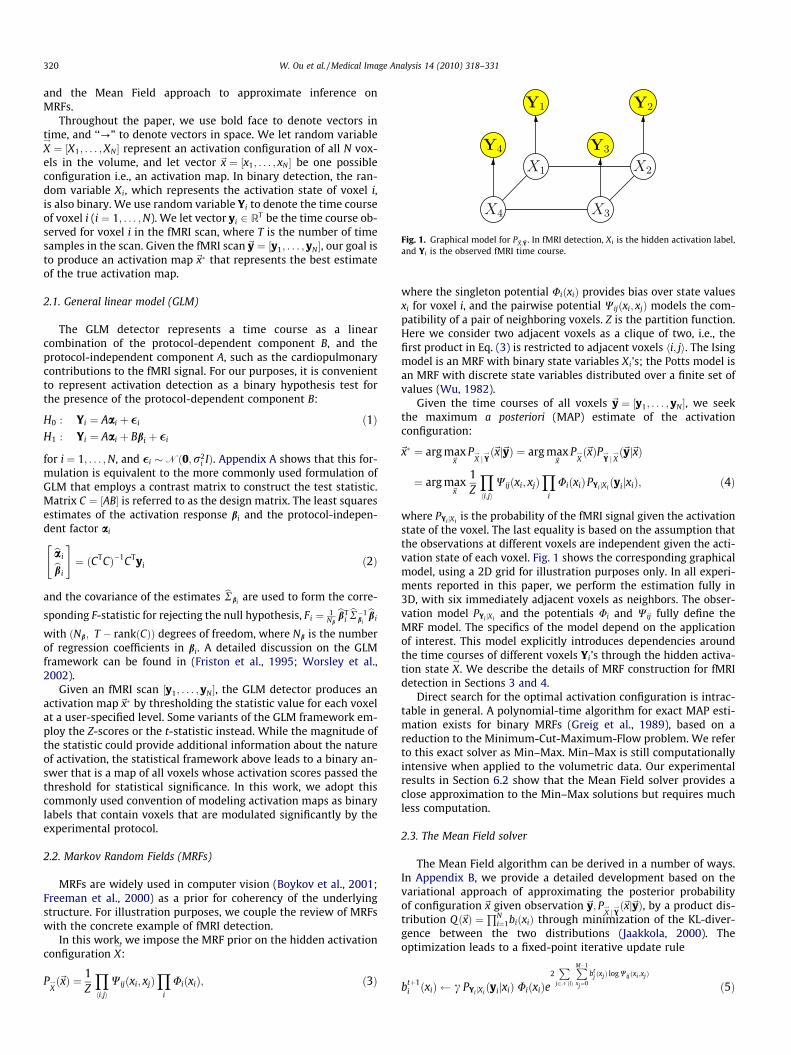
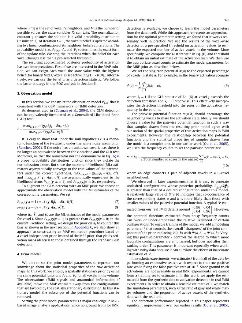
Fig. 1. Graphical model for P~X;~Y . In fMRI detection, Xi is the hidden activation label,and Yi is the observed fMRI time course.

320 W. Ou et al. / Medical Image Analysis 14 (2010) 318–331

and the Mean Field approach to approximate inference onMRFs.

Throughout the paper, we use bold face to denote vectors intime, and ‘‘?” to denote vectors in space. We let random variableX!¼ ½X1; . . . ;XN� represent an activation configuration of all N vox-

els in the volume, and let vector ~x ¼ ½x1; . . . ; xN� be one possibleconfiguration i.e., an activation map. In binary detection, the ran-dom variable Xi, which represents the activation state of voxel i,is also binary. We use random variable Yi to denote the time courseof voxel i (i ¼ 1; . . . ;N). We let vector yi 2 RT be the time course ob-served for voxel i in the fMRI scan, where T is the number of timesamples in the scan. Given the fMRI scan~y ¼ ½y1; . . . ; yN�, our goal isto produce an activation map ~x� that represents the best estimateof the true activation map.

2.1. General linear model (GLM)

The GLM detector represents a time course as a linearcombination of the protocol-dependent component B, and theprotocol-independent component A, such as the cardiopulmonarycontributions to the fMRI signal. For our purposes, it is convenientto represent activation detection as a binary hypothesis test forthe presence of the protocol-dependent component B:

H0 : Yi ¼ Aai þ �i ð1ÞH1 : Yi ¼ Aai þ Bbi þ �i

for i ¼ 1; . . . ;N, and �i �Nð0;r2i IÞ. Appendix A shows that this for-

mulation is equivalent to the more commonly used formulation ofGLM that employs a contrast matrix to construct the test statistic.Matrix C ¼ ½AB� is referred to as the design matrix. The least squaresestimates of the activation response bi and the protocol-indepen-dent factor ai

baibbi

" #¼ ðCTCÞ�1CTyi ð2Þ

and the covariance of the estimates bRbiare used to form the corre-

sponding F-statistic for rejecting the null hypothesis, Fi ¼ 1Nb

bbTibR�1

bibbi

with ðNb; T � rankðCÞÞ degrees of freedom, where Nb is the numberof regression coefficients in bi. A detailed discussion on the GLMframework can be found in (Friston et al., 1995; Worsley et al.,2002).

Given an fMRI scan ½y1; . . . ; yN�, the GLM detector produces anactivation map~x� by thresholding the statistic value for each voxelat a user-specified level. Some variants of the GLM framework em-ploy the Z-scores or the t-statistic instead. While the magnitude ofthe statistic could provide additional information about the natureof activation, the statistical framework above leads to a binary an-swer that is a map of all voxels whose activation scores passed thethreshold for statistical significance. In this work, we adopt thiscommonly used convention of modeling activation maps as binarylabels that contain voxels that are modulated significantly by theexperimental protocol.

2.2. Markov Random Fields (MRFs)

MRFs are widely used in computer vision (Boykov et al., 2001;Freeman et al., 2000) as a prior for coherency of the underlyingstructure. For illustration purposes, we couple the review of MRFswith the concrete example of fMRI detection.

In this work, we impose the MRF prior on the hidden activationconfiguration X

!:

PX!ð~xÞ ¼ 1

Z

Yhi;ji

Wijðxi; xjÞY

i

UiðxiÞ; ð3Þ

where the singleton potential UiðxiÞ provides bias over state valuesxi for voxel i, and the pairwise potential Wijðxi; xjÞ models the com-patibility of a pair of neighboring voxels. Z is the partition function.Here we consider two adjacent voxels as a clique of two, i.e., thefirst product in Eq. (3) is restricted to adjacent voxels hi; ji. The Isingmodel is an MRF with binary state variables Xi’s; the Potts model isan MRF with discrete state variables distributed over a finite set ofvalues (Wu, 1982).

Given the time courses of all voxels ~y ¼ ½y1; . . . ; yN�, we seekthe maximum a posteriori (MAP) estimate of the activationconfiguration:

~x� ¼ arg max~x

PX!j Y!ð~xj~yÞ ¼ arg max

~xP

X!ð~xÞP

Y!j X!ð~yj~xÞ

¼ arg max~x

1Z

Yhi;ji

Wijðxi; xjÞY

i

UiðxiÞPYi jXiðyijxiÞ; ð4Þ

where PYi jXiis the probability of the fMRI signal given the activation

state of the voxel. The last equality is based on the assumption thatthe observations at different voxels are independent given the acti-vation state of each voxel. Fig. 1 shows the corresponding graphicalmodel, using a 2D grid for illustration purposes only. In all experi-ments reported in this paper, we perform the estimation fully in3D, with six immediately adjacent voxels as neighbors. The obser-vation model PYi jXi

and the potentials Ui and Wij fully define theMRF model. The specifics of the model depend on the applicationof interest. This model explicitly introduces dependencies aroundthe time courses of different voxels Yi’s through the hidden activa-tion state X

!. We describe the details of MRF construction for fMRI

detection in Sections 3 and 4.Direct search for the optimal activation configuration is intrac-

table in general. A polynomial-time algorithm for exact MAP esti-mation exists for binary MRFs (Greig et al., 1989), based on areduction to the Minimum-Cut-Maximum-Flow problem. We referto this exact solver as Min–Max. Min–Max is still computationallyintensive when applied to the volumetric data. Our experimentalresults in Section 6.2 show that the Mean Field solver provides aclose approximation to the Min–Max solutions but requires muchless computation.

2.3. The Mean Field solver

The Mean Field algorithm can be derived in a number of ways.In Appendix B, we provide a detailed development based on thevariational approach of approximating the posterior probabilityof configuration~x given observation ~y; P

X!j Y!ð~xj~yÞ, by a product dis-

tribution Qð~xÞ ¼QN

i¼1biðxiÞ through minimization of the KL-diver-gence between the two distributions (Jaakkola, 2000). Theoptimization leads to a fixed-point iterative update rule

btþ1i ðxiÞ c PYi jXi

ðyijxiÞ UiðxiÞe2P

j2NðiÞ

PM�1

xj¼0

btj ðxjÞ log Wijðxi ;xjÞ

ð5Þ


where NðiÞ is the set of voxel i’s neighbors, and M is the number ofpossible values the state variables Xi can take. The normalizationconstant c ensures the solution is a valid probability distribution(it sums to 1). At iteration t þ 1, the voxel’s belief is updated accord-ing to a linear combination of its neighbors’ beliefs at iteration t. Theprobability model (i.e., PYi jXi

; Ui, and Wij) determines the exact formof the update rule. We stop the iterations when the belief for eachvoxel changes less than a pre-selected threshold.

The resulting approximated posterior probability of activationhas two interpretations. First, if we are interested in the MAP solu-tion, we can assign each voxel the state value with the highestbelief (for binary MRFs, voxel i is set active if bið1Þ > bið0Þ). Alterna-tively, we can use the belief bi as a detection statistic. We followthe latter strategy in the ROC analysis in Section 6.

3. Observation model

In this section, we construct the observation model PYi jXithat is

consistent with the GLM framework for fMRI detection.As demonstrated in (Cosman et al., 2004), the GLM detection

can be equivalently formulated as a Generalized Likelihood Ratio(GLR) test:

‘ ¼maxai ;bi ;r2

iNðyi; Bbi þ Aai;r2

i IÞmaxai ;r2

iNðyi; Aai;r2

i IÞ : ð6Þ

It is easy to show that under the null hypothesis ‘ is a mono-tonic function of the F-statistic under the white noise assumption(Rencher, 2002). If the noise has an unknown covariance, there isno longer an equivalence between the F-statistic and the GLR test.Moreover, neither the numerator nor the denominator in Eq. (6) isa proper probability distribution function since they violate thenormalization axiom. But since the maximum likelihood (ML) esti-mators asymptotically converge to the true values of the parame-ters under the correct hypothesis, maxai ;bi ;r2

iNðyi; Bbi þ Aai; r2

i IÞand maxai ;r2

iNðyi; Aai; r2

i IÞ are asymptotically equivalent to thelikelihood terms PYi jXi

ðyijxi ¼ 1Þ and PYi jXiðyijxi ¼ 0Þ, respectively.

To augment the GLM detector with an MRF prior, we choose toapproximate the observation model with the ML estimates of thecorresponding parameters. We set

PYi jXiðyjx ¼ 1Þ ¼Nðy; Bbbi þ Abai; br2

i IÞ; ð7ÞPYi jXi

ðyjx ¼ 0Þ ¼Nðy; Abai; br2i IÞ; ð8Þ

where bai; bbi, and bri are the ML estimates of the model parametersfor voxel i. Since PYi jXi

ðyjx ¼ 1Þ is greater than PYi jXiðyjx ¼ 0Þ in the

current likelihood setting, we design the prior on Xi to counter thisbias as shown in the next section. In Appendix C, we also show anapproach to constructing an MAP estimation procedure based ona voxel-independent prior, instead of the MRF prior, that yields acti-vation maps identical to those obtained through the standard GLMdetection.

4. Prior model

We aim to set the prior model parameters to represent ourknowledge about the statistical properties of the true activationmaps. In this work, we employ a spatially stationary prior by usingthe same potential functions Ui and Wij for all voxels in the volume.The observations (fMRI signals and anatomical information, ifavailable) move the MAP estimate away from the configurationsthat are favored by the spatially stationary distribution. In this sta-tionary model, the subscripts of the potential functions can beremoved.

Setting the prior model parameters is a major challenge in MRF-based image analysis applications. Since no ground truth for fMRI

detection is available, we choose to learn the model parametersfrom the data itself. While this approach represents an approxima-tion for the optimal parameter setting, we found that it works rea-sonably well in practice. We use the results of the voxel-wisedetector at a pre-specified threshold on activation values to esti-mate the expected number of active voxels in the volume. Morespecifically, we compute the GLR statistic in Eq. (6) and thresholdit to obtain an initial estimate of the activation map. We then usethe appropriate voxel counts to estimate the model parameters forthe MRF prior as described below.

We set the singleton potential UðaÞ to the expected percentageof voxels in state a. For example, in the binary activation scenario

UðaÞ ¼ 1N

XN

j¼1

dð~xj � aÞ; ð9Þ

where ~xj ¼ 1 if the GLR statistic of Eq. (6) at voxel j exceeds thedetection threshold and ~xj ¼ 0 otherwise. This effectively incorpo-rates the detection threshold into the prior on the activation fre-quency in the volume.

The pairwise potential function Wða; bÞ should encourage theneighboring voxels to share the activation state. Ideally, we shouldchoose a value for the pairwise potential function in such a waythat samples drawn from the resulting prior model agree withour notion of the spatial properties of true activation maps in fMRIexperiments. However, the relationship between the potentialfunctions and the statistical properties of samples drawn fromthe model is a complex one. In our earlier work (Ou et al., 2005),we used the frequency counts to set the pairwise potentials:

Wða;bÞ ¼ 12ðTotal number of edges in the imageÞ

Xhi;ji

dð~xi � aÞdð~xj � bÞ;

ð10Þ

where an edge connects a pair of adjacent voxels in a 6-voxelneighborhood.

We observed in later experiments that it is easy to generateundesired configurations whose posterior probability, P

X!j Y!ð~xj~yÞ,

is greater than that of a desired configuration under this model.A relatively large value of Wða; bÞ indicates that co-occurrence ofthe corresponding states a and b is more likely than those withsmaller values of the pairwise potential function. A typical W esti-

mated from our real fMRI data is around 0:96 0:040:04 0:96

� �. However,

the potential functions estimated from noisy frequency countscan over- or under-emphasize the relative likelihood of certainconfigurations. To enable training of the model, we add a modelingparameter k that controls the overall ‘‘sharpness” of the joint com-ponent of the prior, replacing Wða; bÞ with eWða; bÞ ¼ Wkða; bÞ. Vary-ing this positive parameter k controls the degree to which morefavorable configurations are emphasized, but does not alter theirranking order. This parameter is important especially when work-ing with noisy data because it can alleviate the effects of inaccurateestimation of W.

In synthetic experiments, we estimate k from half of the data byperforming an exhaustive search with respect to the true positiverate while fixing the false positive rate at 10�3. Since ground truthactivations are not available in real fMRI experiments, we cannotform a training set to estimate k. In this work, we apply the esti-mated k from the synthetic data to activation detection in real fMRIexperiments. In order to obtain a sensible estimate of k, we matchthe simulation parameters, such as the ratio of gray and white mat-ter volumes and the proportion of active voxels, of the syntheticdata with the real one.

The detection performance reported in this paper representssignificant improvement over our earlier results (Ou et al., 2005),


which did not include this modeling parameter k (in other words, itused k ¼ 1). The improvement is particularly large for low SNRdata. The augmented model also achieves a significant improve-ment in the detection accuracy for real fMRI data.

5. Anatomically guided detection

The general nature of the MRF framework enables a straightfor-ward extension of the probabilistic model in the previous sectionto include a tissue type for each voxel. We define V

!¼ ½V1; . . . ;VN�

to be the tissue types of all voxels, and W!¼ ½W1; . . . ;WN� to be

the tissue type observations, e.g., results of automatic segmenta-tion of an MRI scan. Here we model both the hidden tissue typevariables V

!and the observed anatomical labels W

!on the same grid

of the fMRI scan.Now each voxel has two hidden attributes: the activation state

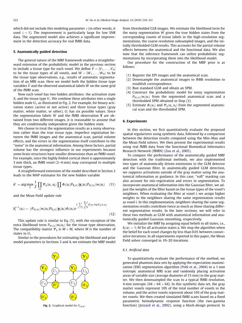
Xi and the tissue type Vi. We combine these attributes into a singlehidden node Ui, as illustrated in Fig. 2. For example, for binary acti-vation states (active or not active) and three tissue types (graymatter, white matter, or other), Ui has six possible values. Sincethe segmentation labels W

!and the fMRI observation Y

!are ob-

tained from two different images, it is reasonable to assume thatthey are conditionally independent given the hidden state.

We choose to treat the segmentation results as a noisy observa-tion rather than the true tissue type. Imperfect registration be-tween the fMRI images and the anatomical scan, partial volumeeffects, and the errors in the segmentation itself contribute to the‘‘noise” in the anatomical information. Among these factors, partialvolume has the strongest influence in our experiments becausesome brain structures have smaller dimensions than an fMRI voxel.For example, since the highly folded cortical sheet is approximately3 mm thick, an fMRI voxel (2–4 mm) may correspond to multipletissue types.

A straightforward extension of the model described in Section 2leads to the MAP estimator for the new hidden variable

~u� ¼ arg max~u

1Z

Yhi;ji

Wijðui; ujÞY

i

UiðuiÞPYi jUiðyijuiÞPWi jUi

ðwijuiÞ ð11Þ

and the Mean Field update rule

btþ1i ðuiÞ cPWi jUi

ðwijuiÞPYi jUiðyijuiÞUiðuiÞe

2P

j2NðiÞ

PM�1

uj¼0

btj ðujÞ log Wijðui ;ujÞ

:

ð12Þ

This update rule is similar to Eq. (5), with the exception of theextra likelihood term PWi jUi

ðwijuiÞ for the tissue type observation.The compatibility matrix Wij is M �M, where M is the number ofstates in Ui.

Similar to the procedures for estimating the likelihood and priormodel parameters in Sections 3 and 4, we estimate the MRF model

Fig. 2. Graphical model for P~U;~Y; ~W .

from thresholded GLR images. We estimate the likelihood term forthe noisy segmentation W

!given the true hidden states from the

corresponding counts of tissue labels in the high-resolution seg-mentations, the coarse resolution subsampled images, and the ini-tially thresholded GLM results. This accounts for the partial volumeeffects between the anatomical and the functional data. We alsonote that the inference framework can utilize probabilistic seg-mentations by incorporating them into the likelihood model.

Our procedure for the construction of the MRF prior is asfollows:

(1) Register the EPI images and the anatomical scan.(2) Downsample the anatomical images to fMRI resolution to

establish correspondence.(3) Run standard GLM and obtain an SPM.(4) Construct the probabilistic model for noisy segmentation

PWi jUiðwijuiÞ from the segmented anatomical scan and a

thresholded SPM obtained in Step (3).(5) Estimate UiðuiÞ and Wijðui;ujÞ from the segmented anatomi-

cal scan and the thresholded SPM.

6. Experiments

In this section, we first quantitatively evaluate the proposedspatial regularizers using synthetic data, followed by a comparisonbetween the detection results computed using the Min–Max andthe Mean Field solvers. We then present the experimental resultsusing real fMRI data from the functional Biomedical InformaticsResearch Network (fBIRN) (Zou et al., 2005).

To compare the performance of the anatomically guided MRFdetection with the traditional methods, we also implementedtwo types of anatomically driven extensions to the GLM detectorand the Gaussian filter. In anatomically guided GLM detection,we suppress activations outside of the gray matter using the ana-tomical information as guidance. In this case, ‘‘soft” masking canalso account for mis-registration and errors in segmentation. Toincorporate anatomical information into the Gaussian filter, we ad-just the weights of the filter based on the tissue types of the voxel’sneighbors. When evaluating the filter at voxel i, we assign higherweights to the neighbors sharing the same segmentation resultsas voxel i. In this implementation, neighbors sharing the same seg-mentation results contribute twice as much as those sharing differ-ent segmentation results. In the later sections, we will refer tothese two methods as GLM with anatomical information and ana-tomically guided Gaussian smoothing, respectively.

We initialize the MRF by assigning equal beliefs to all states, i.e.,biðaÞ ¼ 1=M for all activation states a. We stop the algorithm whenthe belief for each voxel changes by less than 0.01 between consec-utive iterations. In all experiments reported in this paper, the MeanField solver converged in 10–20 iterations.

6.1. Artificial data

To quantitatively evaluate the performance of the method, wegenerated phantom data sets by applying the expectation-maximi-zation (EM) segmentation algorithm (Pohl et al., 2004) to a 1 mmisotropic anatomical MRI scan and randomly placing activationareas of variable size (average diameter of 15 mm) in the gray mat-ter. We then downsampled the scan to a typical fMRI resolution,4 mm isotropic (64 � 64 � 64). In this synthetic data set, the graymatter voxels represent 10% of the total number of voxels in thevolume, and the active voxels represent about 10% of the gray mat-ter voxels. We then created simulated fMRI scans based on a fixedparametric hemodynamic response function (the two-gammafunction) (Jezzard et al., 2002), using a block-design protocol. In

50 100 150 200 250 300Time (sec)

50 100 150 200 250 300Time (sec)

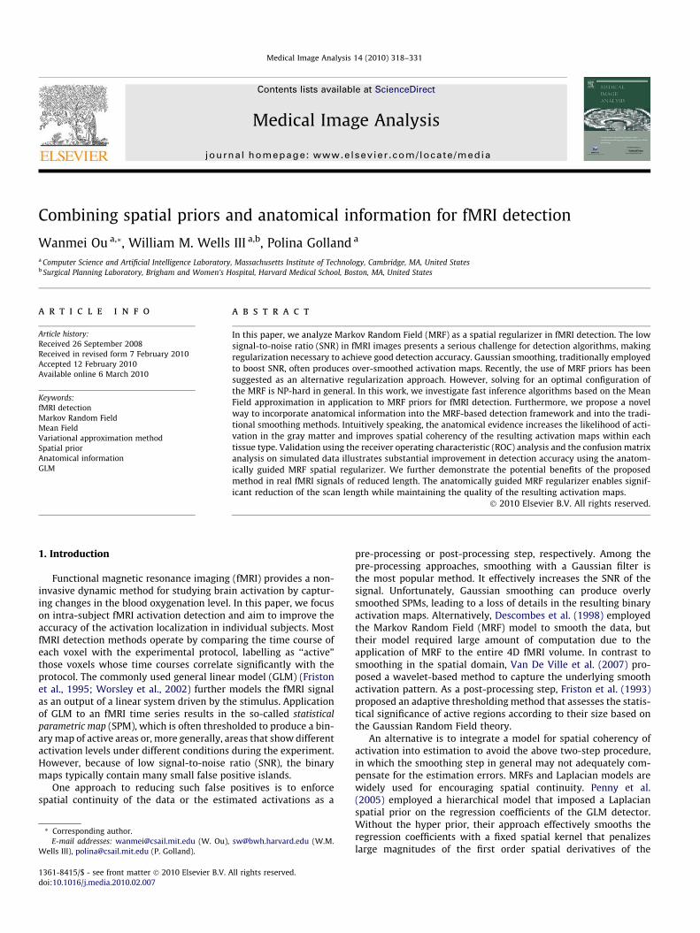
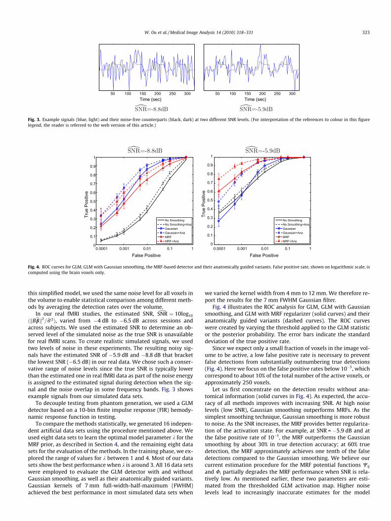
Fig. 3. Example signals (blue, light) and their noise-free counterparts (black, dark) at two different SNR levels. (For interpretation of the references to colour in this figurelegend, the reader is referred to the web version of this article.)

SNR=-8.8dB SNR=-5.9dB

0.0001 0.001 0.01 0.1 10

0.1

0.2

0.3

0.4

0.5

0.6

0.7

0.8

0.9

1

False Positive

True

Pos

itive

No SmoothingNo Smoothing+AnaGaussianGaussian+AnaMRFMRF+Ana

0.0001 0.001 0.01 0.1 10

0.1

0.2

0.3

0.4

0.5

0.6

0.7

0.8

0.9

1

False Positive

True

Pos

itive


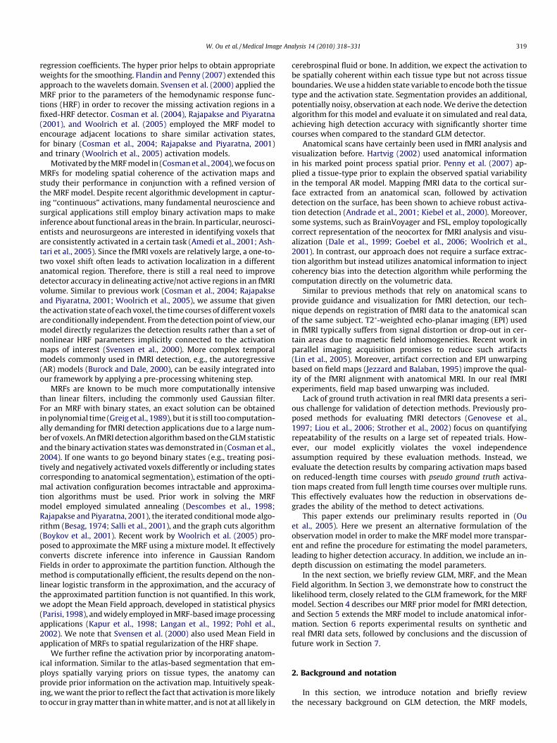
Fig. 4. ROC curves for GLM, GLM with Gaussian smoothing, the MRF-based detector and their anatomically guided variants. False positive rate, shown on logarithmic scale, iscomputed using the brain voxels only.


this simplified model, we used the same noise level for all voxels inthe volume to enable statistical comparison among different meth-ods by averaging the detection rates over the volume.

In our real fMRI studies, the estimated SNR, dSNR ¼ 10log10

ðkBbbk2=br2Þ, varied from �4 dB to �6.5 dB across sessions andacross subjects. We used the estimated SNR to determine an ob-served level of the simulated noise as the true SNR is unavailablefor real fMRI scans. To create realistic simulated signals, we usedtwo levels of noise in these experiments. The resulting noisy sig-nals have the estimated SNR of �5.9 dB and �8.8 dB that bracketthe lowest SNR (�6.5 dB) in our real data. We chose such a conser-vative range of noise levels since the true SNR is typically lowerthan the estimated one in real fMRI data as part of the noise energyis assigned to the estimated signal during detection when the sig-nal and the noise overlap in some frequency bands. Fig. 3 showsexample signals from our simulated data sets.

To decouple testing from phantom generation, we used a GLMdetector based on a 10-bin finite impulse response (FIR) hemody-namic response function in testing.

To compare the methods statistically, we generated 16 indepen-dent artificial data sets using the procedure mentioned above. Weused eight data sets to learn the optimal model parameter k for theMRF prior, as described in Section 4, and the remaining eight datasets for the evaluation of the methods. In the training phase, we ex-plored the range of values for k between 1 and 4. Most of our datasets show the best performance when k is around 3. All 16 data setswere employed to evaluate the GLM detector with and withoutGaussian smoothing, as well as their anatomically guided variants.Gaussian kernels of 7 mm full-width-half-maximum (FWHM)achieved the best performance in most simulated data sets when

we varied the kernel width from 4 mm to 12 mm. We therefore re-port the results for the 7 mm FWHM Gaussian filter.

Fig. 4 illustrates the ROC analysis for GLM, GLM with Gaussiansmoothing, and GLM with MRF regularizer (solid curves) and theiranatomically guided variants (dashed curves). The ROC curveswere created by varying the threshold applied to the GLM statisticor the posterior probability. The error bars indicate the standarddeviation of the true positive rate.

Since we expect only a small fraction of voxels in the image vol-ume to be active, a low false positive rate is necessary to preventfalse detections from substantially outnumbering true detections(Fig. 4). Here we focus on the false positive rates below 10�3, whichcorrespond to about 10% of the total number of the active voxels, orapproximately 250 voxels.

Let us first concentrate on the detection results without ana-tomical information (solid curves in Fig. 4). As expected, the accu-racy of all methods improves with increasing SNR. At high noiselevels (low SNR), Gaussian smoothing outperforms MRFs. As thesimplest smoothing technique, Gaussian smoothing is more robustto noise. As the SNR increases, the MRF provides better regulariza-tion of the activation state. For example, at SNR = �5.9 dB and atthe false positive rate of 10�3, the MRF outperforms the Gaussiansmoothing by about 30% in true detection accuracy; at 60% truedetection, the MRF approximately achieves one tenth of the falsedetections compared to the Gaussian smoothing. We believe ourcurrent estimation procedure for the MRF potential functions Wij

and Ui partially degrades the MRF performance when SNR is rela-tively low. As mentioned earlier, these two parameters are esti-mated from the thresholded GLM activation map. Higher noiselevels lead to increasingly inaccurate estimates for the model

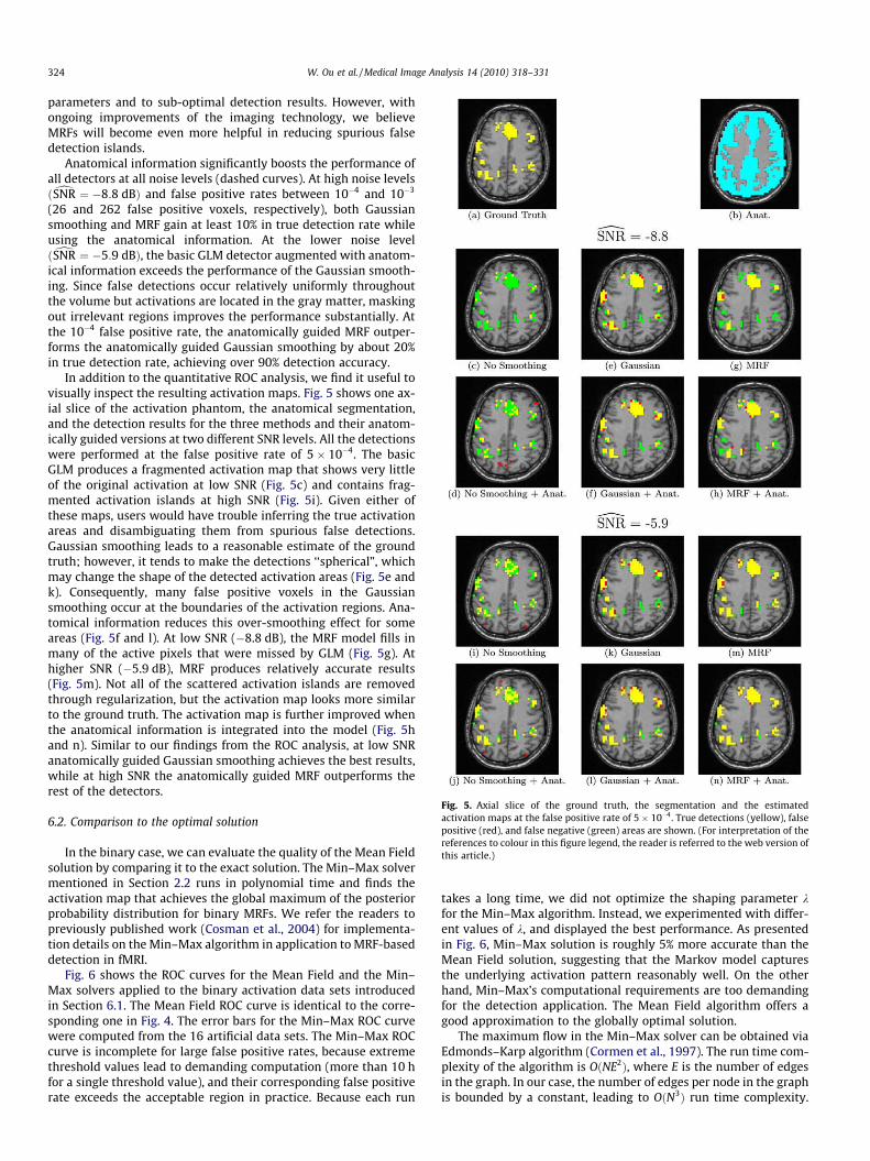
Fig. 5. Axial slice of the ground truth, the segmentation and the estimatedactivation maps at the false positive rate of 5� 10�4. True detections (yellow), falsepositive (red), and false negative (green) areas are shown. (For interpretation of thereferences to colour in this figure legend, the reader is referred to the web version ofthis article.)


parameters and to sub-optimal detection results. However, withongoing improvements of the imaging technology, we believeMRFs will become even more helpful in reducing spurious falsedetection islands.

Anatomical information significantly boosts the performance ofall detectors at all noise levels (dashed curves). At high noise levelsðdSNR ¼ �8:8 dBÞ and false positive rates between 10�4 and 10�3

(26 and 262 false positive voxels, respectively), both Gaussiansmoothing and MRF gain at least 10% in true detection rate whileusing the anatomical information. At the lower noise levelðdSNR ¼ �5:9 dBÞ, the basic GLM detector augmented with anatom-ical information exceeds the performance of the Gaussian smooth-ing. Since false detections occur relatively uniformly throughoutthe volume but activations are located in the gray matter, maskingout irrelevant regions improves the performance substantially. Atthe 10�4 false positive rate, the anatomically guided MRF outper-forms the anatomically guided Gaussian smoothing by about 20%in true detection rate, achieving over 90% detection accuracy.

In addition to the quantitative ROC analysis, we find it useful tovisually inspect the resulting activation maps. Fig. 5 shows one ax-ial slice of the activation phantom, the anatomical segmentation,and the detection results for the three methods and their anatom-ically guided versions at two different SNR levels. All the detectionswere performed at the false positive rate of 5� 10�4. The basicGLM produces a fragmented activation map that shows very littleof the original activation at low SNR (Fig. 5c) and contains frag-mented activation islands at high SNR (Fig. 5i). Given either ofthese maps, users would have trouble inferring the true activationareas and disambiguating them from spurious false detections.Gaussian smoothing leads to a reasonable estimate of the groundtruth; however, it tends to make the detections ‘‘spherical”, whichmay change the shape of the detected activation areas (Fig. 5e andk). Consequently, many false positive voxels in the Gaussiansmoothing occur at the boundaries of the activation regions. Ana-tomical information reduces this over-smoothing effect for someareas (Fig. 5f and l). At low SNR (�8.8 dB), the MRF model fills inmany of the active pixels that were missed by GLM (Fig. 5g). Athigher SNR (�5.9 dB), MRF produces relatively accurate results(Fig. 5m). Not all of the scattered activation islands are removedthrough regularization, but the activation map looks more similarto the ground truth. The activation map is further improved whenthe anatomical information is integrated into the model (Fig. 5hand n). Similar to our findings from the ROC analysis, at low SNRanatomically guided Gaussian smoothing achieves the best results,while at high SNR the anatomically guided MRF outperforms therest of the detectors.

6.2. Comparison to the optimal solution

In the binary case, we can evaluate the quality of the Mean Fieldsolution by comparing it to the exact solution. The Min–Max solvermentioned in Section 2.2 runs in polynomial time and finds theactivation map that achieves the global maximum of the posteriorprobability distribution for binary MRFs. We refer the readers topreviously published work (Cosman et al., 2004) for implementa-tion details on the Min–Max algorithm in application to MRF-baseddetection in fMRI.

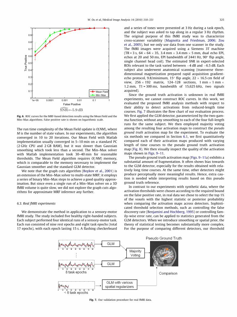
Fig. 6 shows the ROC curves for the Mean Field and the Min–Max solvers applied to the binary activation data sets introducedin Section 6.1. The Mean Field ROC curve is identical to the corre-sponding one in Fig. 4. The error bars for the Min–Max ROC curvewere computed from the 16 artificial data sets. The Min–Max ROCcurve is incomplete for large false positive rates, because extremethreshold values lead to demanding computation (more than 10 hfor a single threshold value), and their corresponding false positiverate exceeds the acceptable region in practice. Because each run

takes a long time, we did not optimize the shaping parameter kfor the Min–Max algorithm. Instead, we experimented with differ-ent values of k, and displayed the best performance. As presentedin Fig. 6, Min–Max solution is roughly 5% more accurate than theMean Field solution, suggesting that the Markov model capturesthe underlying activation pattern reasonably well. On the otherhand, Min–Max’s computational requirements are too demandingfor the detection application. The Mean Field algorithm offers agood approximation to the globally optimal solution.

The maximum flow in the Min–Max solver can be obtained viaEdmonds–Karp algorithm (Cormen et al., 1997). The run time com-plexity of the algorithm is OðNE2Þ, where E is the number of edgesin the graph. In our case, the number of edges per node in the graphis bounded by a constant, leading to OðN3Þ run time complexity.

1e−05 0.0001 0.001 0.01 0.1 10

0.1

0.2

0.3

0.4

0.5

0.6

0.7

0.8

0.9

1

False Positive

True

Pos

itive

Mean FieldMin−Max

Fig. 6. ROC curves for the MRF-based detection results using the Mean Field and theMin–Max algorithms. False positive rate is shown on logarithmic scale.


The run time complexity of the Mean Field update is O(NM), whereM is the number of state values. In our experiments, the algorithmconverged in 10 to 20 iterations. Our Mean Field with Matlabimplementation usually converged in 5–10 min on a standard PC(2 GHz CPU and 2 GB RAM), but it was slower than Gaussiansmoothing which took less than a second. The Min–Max solverwith Matlab implementation took 30–40 min for reasonablethresholds. The Mean Field algorithm requires O( NM) memory,which is comparable to the memory necessary to implement theGaussian smoother and the standard GLM detector.

We note that the graph cuts algorithm (Boykov et al., 2001) isan extension of the Min–Max solver to multi-state MRF; it employsa series of binary Min–Max steps to achieve a good quality approx-imation. But since even a single run of a Min–Max solver on a 3DfMRI volume is quite slow, we did not explore the graph cuts algo-rithms for approximate MRF inference any further.

6.3. Real fMRI experiments

We demonstrate the method in application to a sensory-motorfMRI study. The study included five healthy right-handed subjects.Each subject performed four identical runs of a sensory-motor task.Each run consisted of nine rest epochs and eight task epochs (total17 epochs), with each epoch lasting 15 s. A flashing checkerboard

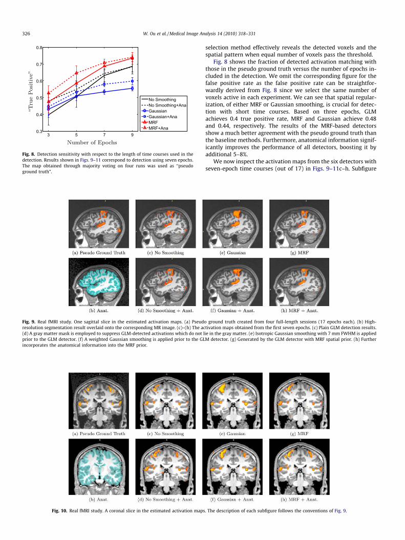
Fig. 7. Our validation proce

and a series of tones were presented at 3 Hz during a task epoch,and the subject was asked to tap along in a regular 3 Hz rhythm.The original purpose of this fMRI study was to characterizecross-scanner variability (Magnotta and Friedman, 2006; Zouet al., 2005), but we only use data from one scanner in the study.The fMRI images were acquired using a Siemens 3T machine(TR = 3 s, 64 � 64 � 35, 3.4 mm � 3.4 mm � 5 mm, dual echo EPI,echos at 20 and 50 ms, EPI bandwidth of 2441 Hz, 90� flip angle,single channel head coil). The estimated SNR in expert-selectedROIs relevant to the task varied between �4 dB and �6.5 dB. Eachsubject also underwent anatomical scanning (transverse three-dimensional magnetization prepared rapid acquisition gradient-echo protocol, 9.8/minimum, 15� flip angle, 22 � 16.5 cm field ofview, 256 � 192 matrix, 124–128 sections, 1 mm � 1 mm �1.2 mm, T1 = 300 ms, bandwidth of 15,625 kHz, two signalsacquired).

Since the ground truth activation is unknown in real fMRIexperiments, we cannot construct ROC curves. In this work, weevaluated the proposed fMRI analysis methods with respect totheir ability to detect activations from reduced-length timecourses. Fig. 7 illustrates the flow chart of our evaluation process.We first applied the GLM detector, parameterized by the two-gam-ma function, without any smoothing to each of the four full-lengthruns for the same subject. We then employed majority votingamong the resulting four activation maps to construct the pseudoground truth activation map for the experiment. To evaluate thesix methods we compared in Section 6.1, we first quantitativelycompared each of their activation maps produced with varyinglength of time courses to the pseudo ground truth activationmap (Fig. 8). We then visually inspect the quality of the activationmaps shown in Figs. 9–11.

The pseudo ground truth activation map (Figs. 9–11a) exhibits asubstantial amount of fragmentation. It often shows bias towardsto the GLM detector, especially for the results obtained with rela-tively long time courses. At the same time, other detectors mightproduce perceptually more meaningful results. Hence, extra cau-tion is needed while interpreting results based on this pseudoground truth reference.

In contrast to our experiments with synthetic data, where theactivation thresholds were chosen according to the required boundon the false positive rate, in real data we chose to select the top 1%of the voxels with the highest statistic or posterior probabilitywhen comparing the activation maps across detectors. Sophisti-cated threshold selection methods, such as controlling the falsediscovery rate (Benjamini and Hochberg, 1995) or controlling fam-ily-wise error rate, can be applied to statistics generated from theGLM detectors. When we introduce smoothing or spatial prior, thetheory of statistical testing becomes substantially more complex.For the purpose of comparing different detectors, our threshold

dure for real fMRI data.

3 5 7 90.3

0.4

0.5

0.6

0.7

0.8


Fig. 8. Detection sensitivity with respect to the length of time courses used in thedetection. Results shown in Figs. 9–11 correspond to detection using seven epochs.The map obtained through majority voting on four runs was used as ‘‘pseudoground truth”.

Fig. 9. Real fMRI study. One sagittal slice in the estimated activation maps. (a) Pseudresolution segmentation result overlaid onto the corresponding MR image. (c)–(h) The ac(d) A gray matter mask is employed to suppress GLM-detected activations which do not lprior to the GLM detector. (f) A weighted Gaussian smoothing is applied prior to the GLincorporates the anatomical information into the MRF prior.

Fig. 10. Real fMRI study. A coronal slice in the estimated activation maps


selection method effectively reveals the detected voxels and thespatial pattern when equal number of voxels pass the threshold.

Fig. 8 shows the fraction of detected activation matching withthose in the pseudo ground truth versus the number of epochs in-cluded in the detection. We omit the corresponding figure for thefalse positive rate as the false positive rate can be straightfor-wardly derived from Fig. 8 since we select the same number ofvoxels active in each experiment. We can see that spatial regular-ization, of either MRF or Gaussian smoothing, is crucial for detec-tion with short time courses. Based on three epochs, GLMachieves 0.4 true positive rate, MRF and Gaussian achieve 0.48and 0.44, respectively. The results of the MRF-based detectorsshow a much better agreement with the pseudo ground truth thanthe baseline methods. Furthermore, anatomical information signif-icantly improves the performance of all detectors, boosting it byadditional 5–8%.

We now inspect the activation maps from the six detectors withseven-epoch time courses (out of 17) in Figs. 9–11c–h. Subfigure

o ground truth created from four full-length sessions (17 epochs each). (b) High-tivation maps obtained from the first seven epochs. (c) Plain GLM detection results.ie in the gray matter. (e) Isotropic Gaussian smoothing with 7 mm FWHM is appliedM detector. (g) Generated by the GLM detector with MRF spatial prior. (h) Further

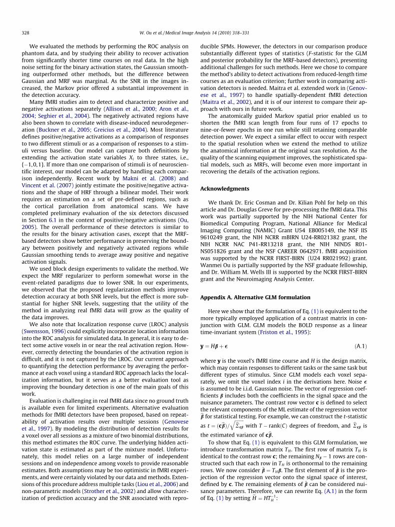
. The description of each subfigure follows the conventions of Fig. 9.

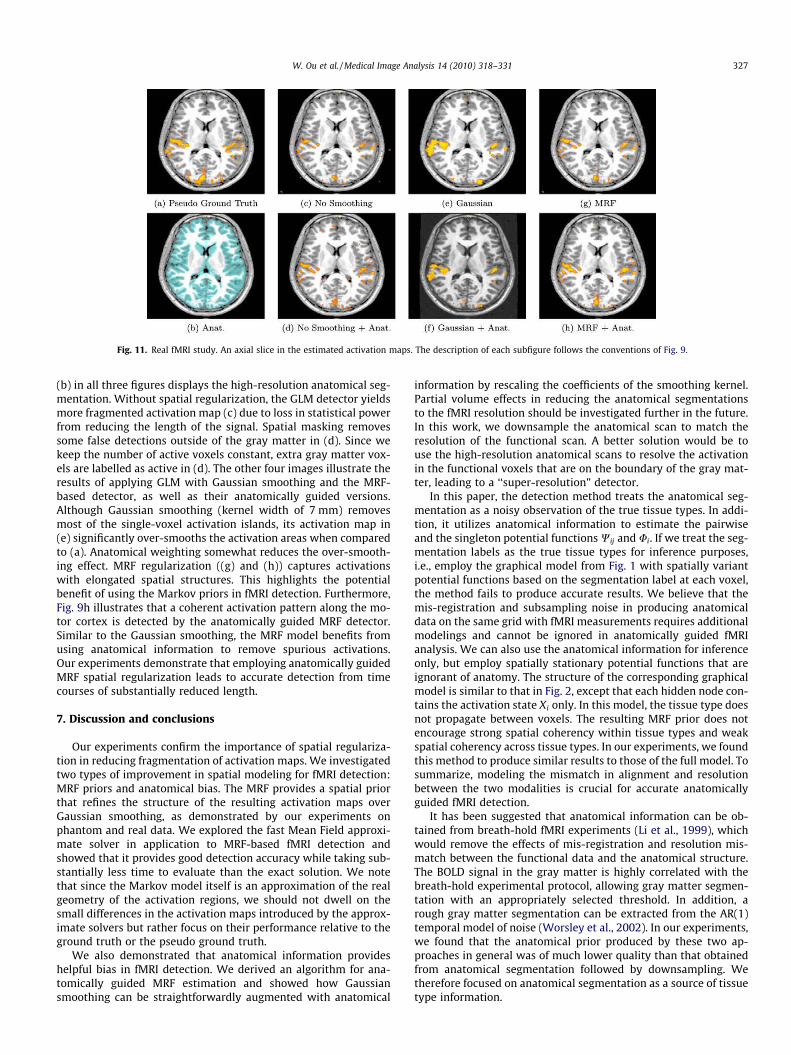
Fig. 11. Real fMRI study. An axial slice in the estimated activation maps. The description of each subfigure follows the conventions of Fig. 9.


(b) in all three figures displays the high-resolution anatomical seg-mentation. Without spatial regularization, the GLM detector yieldsmore fragmented activation map (c) due to loss in statistical powerfrom reducing the length of the signal. Spatial masking removessome false detections outside of the gray matter in (d). Since wekeep the number of active voxels constant, extra gray matter vox-els are labelled as active in (d). The other four images illustrate theresults of applying GLM with Gaussian smoothing and the MRF-based detector, as well as their anatomically guided versions.Although Gaussian smoothing (kernel width of 7 mm) removesmost of the single-voxel activation islands, its activation map in(e) significantly over-smooths the activation areas when comparedto (a). Anatomical weighting somewhat reduces the over-smooth-ing effect. MRF regularization ((g) and (h)) captures activationswith elongated spatial structures. This highlights the potentialbenefit of using the Markov priors in fMRI detection. Furthermore,Fig. 9h illustrates that a coherent activation pattern along the mo-tor cortex is detected by the anatomically guided MRF detector.Similar to the Gaussian smoothing, the MRF model benefits fromusing anatomical information to remove spurious activations.Our experiments demonstrate that employing anatomically guidedMRF spatial regularization leads to accurate detection from timecourses of substantially reduced length.

7. Discussion and conclusions

Our experiments confirm the importance of spatial regulariza-tion in reducing fragmentation of activation maps. We investigatedtwo types of improvement in spatial modeling for fMRI detection:MRF priors and anatomical bias. The MRF provides a spatial priorthat refines the structure of the resulting activation maps overGaussian smoothing, as demonstrated by our experiments onphantom and real data. We explored the fast Mean Field approxi-mate solver in application to MRF-based fMRI detection andshowed that it provides good detection accuracy while taking sub-stantially less time to evaluate than the exact solution. We notethat since the Markov model itself is an approximation of the realgeometry of the activation regions, we should not dwell on thesmall differences in the activation maps introduced by the approx-imate solvers but rather focus on their performance relative to theground truth or the pseudo ground truth.

We also demonstrated that anatomical information provideshelpful bias in fMRI detection. We derived an algorithm for ana-tomically guided MRF estimation and showed how Gaussiansmoothing can be straightforwardly augmented with anatomical

information by rescaling the coefficients of the smoothing kernel.Partial volume effects in reducing the anatomical segmentationsto the fMRI resolution should be investigated further in the future.In this work, we downsample the anatomical scan to match theresolution of the functional scan. A better solution would be touse the high-resolution anatomical scans to resolve the activationin the functional voxels that are on the boundary of the gray mat-ter, leading to a ‘‘super-resolution” detector.

In this paper, the detection method treats the anatomical seg-mentation as a noisy observation of the true tissue types. In addi-tion, it utilizes anatomical information to estimate the pairwiseand the singleton potential functions Wij and Ui. If we treat the seg-mentation labels as the true tissue types for inference purposes,i.e., employ the graphical model from Fig. 1 with spatially variantpotential functions based on the segmentation label at each voxel,the method fails to produce accurate results. We believe that themis-registration and subsampling noise in producing anatomicaldata on the same grid with fMRI measurements requires additionalmodelings and cannot be ignored in anatomically guided fMRIanalysis. We can also use the anatomical information for inferenceonly, but employ spatially stationary potential functions that areignorant of anatomy. The structure of the corresponding graphicalmodel is similar to that in Fig. 2, except that each hidden node con-tains the activation state Xi only. In this model, the tissue type doesnot propagate between voxels. The resulting MRF prior does notencourage strong spatial coherency within tissue types and weakspatial coherency across tissue types. In our experiments, we foundthis method to produce similar results to those of the full model. Tosummarize, modeling the mismatch in alignment and resolutionbetween the two modalities is crucial for accurate anatomicallyguided fMRI detection.

It has been suggested that anatomical information can be ob-tained from breath-hold fMRI experiments (Li et al., 1999), whichwould remove the effects of mis-registration and resolution mis-match between the functional data and the anatomical structure.The BOLD signal in the gray matter is highly correlated with thebreath-hold experimental protocol, allowing gray matter segmen-tation with an appropriately selected threshold. In addition, arough gray matter segmentation can be extracted from the AR(1)temporal model of noise (Worsley et al., 2002). In our experiments,we found that the anatomical prior produced by these two ap-proaches in general was of much lower quality than that obtainedfrom anatomical segmentation followed by downsampling. Wetherefore focused on anatomical segmentation as a source of tissuetype information.


We evaluated the methods by performing the ROC analysis onphantom data, and by studying their ability to recover activationfrom significantly shorter time courses on real data. In the highnoise setting for the binary activation states, the Gaussian smooth-ing outperformed other methods, but the difference betweenGaussian and MRF was marginal. As the SNR in the images in-creased, the Markov prior offered a substantial improvement inthe detection accuracy.

Many fMRI studies aim to detect and characterize positive andnegative activations separately (Allison et al., 2000; Aron et al.,2004; Seghier et al., 2004). The negatively activated regions havealso been shown to correlate with disease-induced neurodegener-ation (Buckner et al., 2005; Greicius et al., 2004). Most literaturedefines positive/negative activations as a comparison of responsesto two different stimuli or as a comparison of responses to a stim-uli versus baseline. Our model can capture both definitions byextending the activation state variables Xi to three states, i.e.,{�1,0,1}. If more than one comparison of stimuli is of neuroscien-tific interest, our model can be adapted by handling each compar-ison independently. Recent work by Makni et al. (2008) andVincent et al. (2007) jointly estimate the positive/negative activa-tions and the shape of HRF through a bilinear model. Their workrequires an estimation on a set of pre-defined regions, such asthe cortical parcellation from anatomical scans. We havecompleted preliminary evaluation of the six detectors discussedin Section 6.1 in the context of positive/negative activations (Ou,2005). The overall performance of these detectors is similar tothe results for the binary activation cases, except that the MRF-based detectors show better performance in preserving the bound-ary between positively and negatively activated regions whileGaussian smoothing tends to average away positive and negativeactivation signals.

We used block design experiments to validate the method. Weexpect the MRF regularizer to perform somewhat worse in theevent-related paradigms due to lower SNR. In our experiments,we observed that the proposed regularization methods improvedetection accuracy at both SNR levels, but the effect is more sub-stantial for higher SNR levels, suggesting that the utility of themethod in analyzing real fMRI data will grow as the quality ofthe data improves.

We also note that localization response curve (LROC) analysis(Swensson, 1996) could explicitly incorporate location informationinto the ROC analysis for simulated data. In general, it is easy to de-tect some active voxels in or near the real activation region. How-ever, correctly detecting the boundaries of the activation region isdifficult, and it is not captured by the LROC. Our current approachto quantifying the detection performance by averaging the perfor-mance at each voxel using a standard ROC approach lacks the local-ization information, but it serves as a better evaluation tool asimproving the boundary detection is one of the main goals of thiswork.

Evaluation is challenging in real fMRI data since no ground truthis available even for limited experiments. Alternative evaluationmethods for fMRI detectors have been proposed, based on repeat-ability of activation results over multiple sessions (Genoveseet al., 1997). By modeling the distribution of detection results fora voxel over all sessions as a mixture of two binomial distributions,this method estimates the ROC curve. The underlying hidden acti-vation state is estimated as part of the mixture model. Unfortu-nately, this model relies on a large number of independentsessions and on independence among voxels to provide reasonableestimates. Both assumptions may be too optimistic in fMRI experi-ments, and were certainly violated by our data and methods. Exten-sions of this procedure address multiple tasks (Liou et al., 2006) andnon-parametric models (Strother et al., 2002) and allow character-ization of prediction accuracy and the SNR associated with repro-

ducible SPMs. However, the detectors in our comparison producesubstantially different types of statistics (F-statistic for the GLMand posterior probability for the MRF-based detectors), presentingadditional challenges for such methods. Here we chose to comparethe method’s ability to detect activations from reduced-length timecourses as an evaluation criterion; further work in comparing acti-vation detectors is needed. Maitra et al. extended work in (Genov-ese et al., 1997) to handle spatially-dependent fMRI detection(Maitra et al., 2002), and it is of our interest to compare their ap-proach with ours in future work.

The anatomically guided Markov spatial prior enabled us toshorten the fMRI scan length from four runs of 17 epochs tonine-or-fewer epochs in one run while still retaining comparabledetection power. We expect a similar effect to occur with respectto the spatial resolution when we extend the method to utilizethe anatomical information at the original scan resolution. As thequality of the scanning equipment improves, the sophisticated spa-tial models, such as MRFs, will become even more important inrecovering the details of the activation regions.

Acknowledgments

We thank Dr. Eric Cosman and Dr. Kilian Pohl for help on thisarticle and Dr. Douglas Greve for pre-processing the fMRI data. Thiswork was partially supported by the NIH National Center forBiomedical Computing Program, National Alliance for MedicalImaging Computing (NAMIC) Grant U54 EB005149, the NSF IIS9610249 grant, the NIH NCRR mBIRN U24-RR021382 grant, theNIH NCRR NAC P41-RR13218 grant, the NIH NINDS R01-NS051826 grant and the NSF CAREER 0642971. fMRI acquisitionwas supported by the NCRR FIRST-BIRN (U24 RR021992) grant.Wanmei Ou is partially supported by the NSF graduate fellowship,and Dr. William M. Wells III is supported by the NCRR FIRST-BIRNgrant and the Neuroimaging Analysis Center.

Appendix A. Alternative GLM formulation

Here we show that the formulation of Eq. (1) is equivalent to themore typically employed application of a contrast matrix in con-junction with GLM. GLM models the BOLD response as a lineartime-invariant system (Friston et al., 1995):

y ¼ Hbþ � ðA:1Þ

where y is the voxel’s fMRI time course and H is the design matrix,which may contain responses to different tasks or the same task butdifferent types of stimulus. Since GLM models each voxel sepa-rately, we omit the voxel index i in the derivations here. Noise �is assumed to be i.i.d. Gaussian noise. The vector of regression coef-ficients b includes both the coefficients in the signal space and thenuisance parameters. The contrast row vector c is defined to selectthe relevant components of the ML estimate of the regression vectorbb for statistical testing. For example, we can construct the t-statistic

as t ¼ ðcbbÞ= ffiffiffiffiffiffiffiffibRcb

qwith T � rankðCÞ degrees of freedom, and bRcb is

the estimated variance of cbb.To show that Eq. (1) is equivalent to this GLM formulation, we

introduce transformation matrix TH . The first row of matrix TH isidentical to the contrast row c; the remaining Nb � 1 rows are con-structed such that each row in TH is orthonormal to the remainingrows. We now consider ~b ¼ THb. The first element of ~b is the pro-jection of the regression vector onto the signal space of interest,defined by c. The remaining elements of ~b can be considered nui-sance parameters. Therefore, we can rewrite Eq. (A.1) in the formof Eq. (1) by setting eH ¼ HT�1

H :


y ¼ Hbþ � ¼ eH~bþ � ¼ eHð1Þ~bð1Þ þ eHð½2;��;Nb �Þ~bð½2;��;Nb �Þ þ �: ðA:2Þ

The first term in the resulting sum corresponds to the signal spacecomponents. The second term in the sum represents contributionsorthogonal to the signal space of interest.

Appendix B. Mean Field derivation

In this appendix, we demonstrate one possible derivation of theMean Field iteration as a variational approximation of the originalMAP problem, closely following the development in (Jaakkola,2000). The basic idea is to approximate the posterior probabilityP

X!j Y!ð~xj~yÞ by a simpler distribution Qð~x;~bÞ ¼

QNi¼1biðxiÞ through min-

imizing the KL-divergence between them and to use the mode ofQð�;~bÞ as an approximation for the mode of P

X!j Y!ð�j~yÞ. ~b ¼

½b1; b2; . . . ; bN� is the vector of belief functions: biðaÞ denotes the

probability that voxel i is in state a. Clearly,PM�1

a¼0 biðaÞ ¼ 1, whereM is the number of possible values that the state variable Xi cantake. For example, M ¼ 2 for binary MRFs. We note that the result-ing distribution Qð�;~bÞ implicitly depends on the observations ~y.

The KL-divergence

DðQkPX!j Y!Þ ¼

X~x

Qð~xÞ logQð~xÞ

PX!j Y!ð~xj~yÞ

0@ 1A ðB:1Þ

serves as a distance between Qð�;~bÞ and PX!j~Yð�j~yÞ; it is non-negative

and is equal to zero only if Q ¼ PX!j Y!. As an aside, the statistical

inference theory implies that we should minimize the KL-diver-gence DðP

X!j Y!kQÞ, which often leads to intractable problems. To

overcome this difficulty, variational methods are usually formu-lated as a minimization of the KL-divergence DðQkP

X!j Y!Þ.

It is easy to see that the minimum of DðQð�;~bÞkPX!j Y!Þ is achieved

for the same belief vector ~b� that minimizes the so-called freeenergy,

FMFð~bÞ ¼ D QkPX!j Y!

� �� log P

Y!ð~yÞ

� �� logðZÞ ðB:2Þ

since the last two terms are independent of~b. Substituting the def-initions for Qð~x;~bÞ and for P

X!j~Yð~xj~yÞ, we obtain,

FMFð~bÞ ¼ �X

i

Xj2NðiÞ

XM�1

xi¼0

XM�1

xj¼0

biðxiÞbjðxjÞ logðWijðxi; xjÞÞ

þX

i

XM�1

xi¼0

biðxiÞ logðbiðxiÞÞ � logðPYi jXiðyijxiÞUiðxiÞÞ

� �ðB:3Þ

leading to the following constrained optimization problem:

~b� ¼ arg min~b

FMFð~bÞ ðB:4Þ

s:t:XM�1

a¼0

biðaÞ ¼ 1; 8i:

Using Lagrange multipliers, we reduce the problem above tominimize

Jð~bÞ ¼ �X

i

Xj2NðiÞ

XM�1

xi¼0

XM�1

xj¼0

biðxiÞbjðxjÞ logðWijðxi; xjÞÞ

þX

i

XM�1

xi¼0

biðxiÞ logðbiðxiÞÞ � logðPYi jXiðyijxiÞUiðxiÞÞ

� �þX

i

ni

XM�1

xi¼0

ðbiðxiÞ � 1Þ:

Differentiating with respect to bkðxkÞ yields

@Jð~bÞ@bkðxkÞ

¼ �2X

j2NðkÞ

XM�1

xj¼0

bkðxkÞbjðxjÞ logðWkjðxk; xjÞÞ þ 1

þ logðbkðxkÞÞ � logðPYk jXkðykjxkÞUkðxkÞÞ þ nk: ðB:5Þ

By setting the derivatives to zero and manipulating the expres-sion above, we arrive at the fixed-point iteration for the belieffunctions

bkðxkÞ e1þnk PYk jXkðykjxkÞUkðxkÞe

2P

j2NðkÞ

PM�1

xj¼0

bjðxjÞ logðWkjðxk ;xjÞÞ

ðB:6Þ

that immediately leads to the Mean Field update rule of Eq. (5) if weset c ¼ e1þnk .

Appendix C. Equivalence to the joint MAP solution

In this appendix, we present the connection between the MAPsolution and the classical GLM inference in the binary activationscenario. In particular, we show that for a prior that models all vox-els independently, there is a setting of the prior that forces the MAPsolution to coincide with the classical solution. Furthermore, thetwo-step estimation procedure we outlined in Section 3, whichfirst finds the ML estimates of the GLM parameters fa; b; r2gand then uses them in the MAP estimation of the state variablesX, is asymptotically equivalent to the optimal simultaneous MAPestimation of the activation state and the regression parametersin the case of the voxel-wise independent prior.

To simplify the derivations, we let H0i ¼ fai;r2i g be the param-

eters of the likelihood under H0 for voxel i, H1i ¼ fai; bi;r2i g be the

parameters of the likelihood under H1 for voxel i, bHMAP0i ð bHML

0i Þ andbHMAP1i ð bHML

1i Þ be the MAP (ML) estimates of H0i and H1i, respectively.The activation state estimate obtained through the joint MAP esti-mation of the activation state and the GLM parameters

f~x�~h�0 ~h1�g ¼ arg max

~x;~h0 ;~h1

P~X;~H0 ;~H1 j~Yð~x;

~h0;~h1j~yÞ

¼ arg max~x;~h0 ;

~h1

P~X;~H0 ;~H1 ;

~Yð~x;~h0;~h1;~yÞ ðC:1Þ

can also be expressed as

~x� ¼ arg max~x

max~h0 ;

~h1

P~X;~H0 ;~H1 ;

~Yð~x;~h0;~h1;~yÞ ðC:2Þ

¼ arg max~x

P~Xð~xÞYN

i¼1

maxh0 ;h1

PH0i ;H1i ;Yi jXiðh0; h1; yijxiÞ ðC:3Þ

For a voxel-wise independent prior P~Xð~xÞ ¼QN

i¼1PXiðxiÞ, the problem

above can be solved for each voxel separately. In the remainder ofthis section, we omit the voxel index i.

x� ¼ arg maxx2f0;1g

PXðxÞmaxh0 ;h1

PH0 ;H1 ;YjXðh0; h1; yjxÞ ðC:4Þ

¼ arg maxx2f0;1g

PXðxÞmaxh

PY;Hx jXðy; hjxÞ ðC:5Þ

¼ arg maxx2f0;1g

PXðxÞPY;Hx jXðy; bHMAPx jxÞ ðC:6Þ

¼ arg maxx2f0;1g

PXðxÞPYjHx ;Xðyj bHMAPx ; xÞ ðC:7Þ

� arg maxx2f0;1g

PXðxÞPYjHx ;Xðyj bHMLx ; xÞ ðC:8Þ


We obtained Eq. (C.6) by assuming a uniform prior distribution forHx. Eq. (C.8) is true asymptotically as the number of time points in atime course increases. Alternatively, we can express Eq. (C.8) interms of hypothesis testing:

PYjXðyj bHML1 ; x ¼ 1Þ


H1

?

H0

PXðx ¼ 0ÞPXðx ¼ 1Þ : ðC:9Þ

As shown in (Rencher, 2002), the left-hand side of Eq. (C.9) is amonotonic function of the F-statistic. Thus, we obtain the corre-sponding hypothesis testing threshold, g, according to the selectedp value threshold in the classical GLM procedure:



H1

?

H0

g: ðC:10Þ

This implies that selecting PXðx ¼ 0Þ ¼ g1þg and PXðx ¼ 1Þ ¼ 1

1þgcauses the MAP with independent prior and the classical inferencesto produce identical results.

References

Allison, J.D., Meador, K.J., Loring, D.W., Figueroa, R.E., Wright, J.C., 2000. FunctionalMRI cerebral activation and deactivation during finger movement. Neurology54, 135–142.

Amedi, A., Malach, R., Hendler, T., Peled, S., Zohary, E., 2001. Visuo-haptic object-related activation in the ventral visual pathway. Nature Neuroscience 4, 324–330.

Andrade, A., Kherif, F., Mangin, J.-F., Worsley, K.J., Paradis, A.-L., Simon, O., Dehaene,S., Bihan, D.L., Poline, J.-B., 2001. Detection of fMRI activation using corticalsurface mapping. Human Brain Mapping 12, 79–93.

Aron, A.R., Shohamy, D., Clark, J., Myers, C., Gluck, M.A., Poldrack, R.A., 2004. Humanmidbrain sensitivity to cognitive feedback and uncertainty during classificationlearning. Journal of Neurophysiology 92, 1144–1152.

Ashtari, M., Perrine, K., Elbaz, R., Syed, U., Thaden, E., McIlree, C., Dolgoff-Kaspar, R.,Clarke, T., Diamond, A., Ettinger, A., 2005. Mapping the functional anatomy ofsentence comprehension and application to presurgical evaluation of patientswith brain tumor. American Journal of Neuroradiology 26, 1461–1468.

Benjamini, J., Hochberg, Y., 1995. Controlling the false discovery rate: a practical andpowerful approach to multiple testing. Journal of the Royal Statistical SocietySeries B 57, 289–300.

Besag, J., 1974. Spatial interaction and the statistical analysis of lattice systems.Journal of the Royal Statistical Society Series B 36, 192–236.

Boykov, Y., Veksler, O., Zabih, R., 2001. Fast approximate energy minimization viagraph cuts. IEEE Transactions on Pattern Analysis and Machine Intelligence 23,1222–1239.

Buckner, R.L., Snyder, A.Z., Shannon, B.J., LaRossa, G., Sachs, R., Fotenos, A.F., Sheline,Y.I., Klunk, W.E., Mathis, C.A., Morris, J.C., Mintun, M.A., 2005. Molecular,structural, and functional characterization of Alzheimer’s disease: evidence fora relationship between default activity, amyloid, and memory. Journal ofNeuroscience 25, 7709–7717.

Burock, M.A., Dale, A.M., 2000. Estimation and detection of event-related fMRIsignals with temporally correlated noise: a statistically efficient and unbiasedapproach. Human Brain Mapping 11, 249–260.

Cormen, T.H., Leiserson, C.E., Rivest, R.L., 1997. Introduction to Algorithms. The MITPress and McGraw-Hill.

Cosman, E.R., Fisher, J.W., Wells, W.M., 2004. Exact MAP activity detection in fMRIusing a GLM with an Ising spatial prior. In: Proceedings of the Medical ImageComputing and Computer-Assisted Intervention, LNCS, vol. 3217, pp. 703–710.

Dale, A.M., Fischl, B., Sereno, M.I., 1999. Cortical surface-based analysis. I:segmentation and surface reconstruction. NeuroImage 9, 179–194.

Descombes, X., Kruggel, F., von Cramon, D.Y., 1998. Spatio-temporal fMRI analysisusing Markov random fields. IEEE Transactions on Medical Imaging 17, 1028–1039.

Flandin, G., Penny, W.D., 2007. Bayesian fMRI data analysis with sparse spatial basisfunction priors. NeuroImage 34, 1108–1125.

Freeman, W., Pasztor, E.C., Carmichael, O.T., 2000. Learning low-level vision.International Journal of Computer Vision 40, 25–47.

Friston, K.J., Worsley, K.J., Frackowiak, R.S.J., Massiotta, J.C., Evans, A.C., 1993.Assessing the significance of local activations using their spatial extent. HumanBrain Mapping 1, 210–220.

Friston, K.J., Holmes, A.P., Worsley, K.J., Poline, J.-B., Frith, C.D., Frackowiak, R.S.J.,1995. Statistical parametric maps in functional imaging: a general linearapproach. Human Brain Mapping 2, 189–210.

Genovese, C.R., Noll, D.C., Eddy, W.F., 1997. Estimating test–retest reliability infunctional MR imaging. I: statistical methodology. Magnetic Resonance inMedicine 38, 497–507.

Goebel, R., Esposito, F., Formisano, E., 2006. Analysis of functional imageanalysis contest (FIAC) data with brainvoyager QX: from single-subject tocortically aligned group general linear model analysis and self-organizinggroup independent component analysis. Human Brain Mapping 27, 392–401.

Greicius, M.D., Srivastava, G., Reiss, A.L., Menon, V., 2004. Default-mode networkactivity distinguishes Alzheimer’s disease from healthy aging: evidence fromfunctional MRI. National Academy of Sciences 101, 4637–4642.

Greig, D.M., Porteous, B.T., Gramon, D.Y., 1989. Exact maximum a posterioriestimation for binary images. Journal of the Royal Statistical Society Series B 51,271–279.

Hartvig, N.V., 2002. A stochastic geometry model for functional magnetic resonanceimages. Scandinavian Journal of Statistics 29, 333–353.

Jaakkola, T., 2000. Tutorial on variational approximation methods. Advanced MeanField Methods: Theory and Practice. MIT Press.

Jezzard, P., Balaban, R.S., 1995. Correction for geometric distortion in echo planarimages from B0 field variations. Magnetic Resonance in Medicine 34, 65–73.

Jezzard, F., Matthews, P.M., Smith, S.M., 2002. Functional MIR – An Introduction toMethods. Oxford University Press, Oxford.

Kapur, T., Grimson, W.E.L., Wells, W.M., Kikinis, R., 1998. Enhanced spatial priors forsegmentation of magnetic resonance imagery. In: Proceedings of the MedicalImage Computing and Computer-Assisted Intervention, LNCS, vol. 1496, pp.457–468.

Kiebel, S.J., Goebel, R., Friston, K.J., 2000. Anatomically informed basis functions.NeuroImage 11, 656–667.

Langan, D.A., Molnar, K.J., Modestino, J.W., Zhang, J., 1992. Use of the mean-fieldapproximation in an EM-based approach to unsupervised stochastic model-based image segmentation. In: Proceedings of the IEEE International Conferenceon Acoustics, Speech, and Signal Processing, vol. 3, pp. 57–60.

Li, T.Q., Kastrup, A., Takahashi, A.M., Moseley, M.E., 1999. Function MRI of humanbrain during breath holding by BOLD and FAIR techniques. NeuroImage 9, 243–249.

Lin, F.S., Huang, T.Y., Chen, N.K., Wang, F.N., Stufflebeam, S.M., Belliveau, J.W., Wald,L.L., Kwong, K.K., 2005. Functional MRI using regularized parallel imagingacquisition. Magnetic Resonance in Medicine 54, 343–353.

Liou, M., Su, H.R., Lee, J.D., Aston, J.A.D., Tsai, A.C., Cheng, P.E., 2006. A methodfor generating reproducible evidence in fMRI studies. NeuroImage 29, 383–395.

Magnotta, V.A., Friedman, L., 2006. FIRST BIRN measurement of signal-to-noise andcontrast-to-noise in the fBIRN multi-center imaging study. Journal of DigitalImaging 19, 140–147.

Maitra, R., Roys, S., Gullapalli, R., 2002. Test–retest reliability estimation offunctional MRI data. Magnetic Resonance in Medicine 48, 62–70.

Makni, S., Idier, J., Vincent, T., Thirion, B., Dehaene-Lambertz, G., Ciuciu, P., 2008. Afully Bayesian approach to the parcel-based detection-estimation of brainactivity in fMRI. NeuroImage 41, 941–969.

Ou, W., Golland, P., 2005. From spatial regularization to anatomical priors in fMRIanalysis. In: Proceedings of the IPMI, LNCS, vol. 3565, pp. 88–100.

Ou, W., 2005. fMRI detection with spatial regularization. MIT Master Thesis.Parisi, G., 1998. Statistical Field Theory. Addison-Wesley.Penny, W.D., Trujillo-Barreto, N.J., Friston, K.J., 2005. Bayesian fMRI time series

analysis with spatial priors. NeuroImage 24, 350–362.Penny, W.D., Flandin, G., Trujillo-Barreto, N.J., 2007. Bayesian comparison of

spatially regularised general linear models. Human Brain Mapping 28, 275–293.

Pohl, K.M., Wells, W.M., Guimond, A., Kasai, K., Shenton, M.E., Kikinis, R., Grimson,W.E.L., Warfield, S.K., 2002. Incorporating non-rigid registration intoexpectation maximization algorithm to segment MR images. In: Proceedingsof the Medical Image Computing and Computer-Assisted Intervention, LNCS,vol. 2488, pp. 564–571.

Pohl, K.M., Bouix, S., Kikinis, R., Grimson, W.E.L., 2004. Anatomical guidedsegmentation with non-stationary tissue class distributions in an expectation-maximization framework. In: Proceedings of the IEEE Symposium onBiomedical Imaging, vol. 1, pp. 81–84.

Rajapakse, J.C., Piyaratna, J., 2001. Bayesian approach to segmentation of statisticalparametric maps. IEEE Transactions on Biomedical Engineering 48, 1186–1194.

Rencher, A.C., 2002. Methods of Multivariate Analysis. Wiley.Salli, E., Aronen, H.J., Savolainen, S., Korvenoja, A., Visa, A., 2001. Contextual

clustering for analysis of functional MRI data. IEEE Transactions on MedicalImaging 20, 403–414.

Seghier, M.L., Lazeyras, F., Zimine, S., Maier, S.E., Hanquinet, S., Delavelle, J.,Volpe, J.J., Huppi, P.S., 2004. Combination of event-related fMRI anddiffusion tensor imaging in an infant with perinatal stroke. NeuroImage21, 463–472.

Strother, S.C., Anderson, J., Hansen, L.K., Kjems, U., Kustra, R., Sidtis, J., Frutiger, S.,Muley, S., LaConte, S., Rottenberg, D., 2002. The quantitative evaluation offunctional neuroimaging experiments: the NPAIRS data analysis framework.NeuroImage 15, 747–771.

Svensen, M., Kruggel, F., von Cramon, D.Y., 2000. Probabilistic modeling of single-trial fMRI data. IEEE Transactions on Medical Imaging 19, 25–35.

Swensson, R.G., 1996. Unified measurement of observer performance indetecting and localizing target objects on images. Medical Physics 23, 1025–1709.

Van De Ville, D., Seghier, M.L., Lazeyras, F., Blu, T., Unser, M., 2007. WSPM: wavelet-based statistical parametric mapping. NeuroImage 37, 1205–1217.


Vincent, T., Ciuciu, P., Idier, J., 2007. Spatial mixture modelling for the jointdetection-estimation of brain activity in fMRI. In: Proceedings of the ICASSP,vol. 1, pp. 325–328.

Woolrich, M.W., Ripley, B.D., Brady, M., Smith, S.M., 2001. Temporal autocorrelationin univariate linear modelling of fMRI data. NeuroImage 14, 1370–1386.

Woolrich, M.W., Behrens, T.E., Beckmann, C.F., Smith, S.M., 2005. Mixture modelswith adaptive spatial regularization for segmentation with an application tofMRI data. IEEE Transactions on Medical Imaging 24, 1–11.

Worsley, K.J., Liao, C.H., Aston, J., Petre, V., Duncan, G.H., Morales, F., Evans, A.C.,2002. A general statistical analysis for fMRI data. NeuroImage 15, 1–15.

Wu, F., 1982. The Potts model. Reviews of Modern Physics 54, 235–268.Zou, K.H., Greve, D.N., Wang, M., Pieper, S.D., Warfield, S.K., White, N.S., Manandhar,

S., Brown, G.G., Vangel, M.G., Kikinis, R., Wells, W.M., 2005. Reproducibility offunctional MR imaging: preliminary results of prospective multi-institutionalstudy performed by biomedical informatics research network. Radiology 237,781–789.

Documents

Combining spatial priors and anatomical information for