Combining Novelty-Guided and Heuristic-Guided Searchai.cs.unibas.ch/papers/theses/maggi-master-16.pdf · Combining Novelty-Guided and Heuristic-Guided Search Master Thesis Natural

Combining Novelty-Guided andHeuristic-Guided Search

Master Thesis

Natural Science Faculty of the University of Basel

Department of Mathematics and Computer Science

Artificial Intelligence

ai.cs.unibas.ch

Examiner: Prof. Dr. Malte Helmert

Supervisor: Dr. Thomas Keller

Dario Maggi

[email protected]

2011-056-181

17.7.2016

Acknowledgments

First, I would like to thank Prof. Dr. Malte Helmert for the opportunity to write this thesis

in the Artificial Intelligence group of the University of Basel. Many thanks to the Artificial

Intelligence group for their help and a special thanks to Dr. Thomas Keller for his supervision

and guidance.

I am thankful to Nir Lipovetzky for answering my questions considering their implementa-

tions. Thanks to the Universitatsrechenzentrum for providing the cluster infrastructure for the

experiments and a special thanks to Pablo Escobar Lopez for helping with compilation problems

on the cluster.

Last but not least, I want to thank my family and friends for their support and encourage-

ment.

Abstract

Greedy Best-First Search (GBFS) is a prominent search algorithm to find solutions for planning

tasks. GBFS chooses nodes for further expansion based on a distance-to-goal estimator, the

heuristic. This makes GBFS highly dependent on the quality of the heuristic. Heuristics often

face the problem of producing Uninformed Heuristic Regions (UHRs). GBFS additionally suffers

the possibility of simultaneously expanding nodes in multiple UHRs.

In this thesis we change the heuristic approach in UHRs. The heuristic was unable to guide

the search and so we try to expand novel states to escape the UHRs. The novelty measures how

“new” a state is in the search.

The result is a combination of heuristic and novelty guided search, which is indeed able to

escape UHRs quicker and solve more problems in reasonable time.

Table of Contents

Acknowledgments ii

Abstract iii

1 Introduction 1

2 Background 3

2.1 Planning . . . . . . . . . . . . . . . . . . . . . . . . . . . . . . . . . . . . . . . . . 3

2.2 Search . . . . . . . . . . . . . . . . . . . . . . . . . . . . . . . . . . . . . . . . . . 5

2.2.1 Greedy Best First Search (GBFS) . . . . . . . . . . . . . . . . . . . . . . 6

2.2.2 Local Exploration . . . . . . . . . . . . . . . . . . . . . . . . . . . . . . . 7

2.3 Novelty Based Algorithms . . . . . . . . . . . . . . . . . . . . . . . . . . . . . . . 7

2.3.1 Iterated Width (IW) . . . . . . . . . . . . . . . . . . . . . . . . . . . . . . 8

2.3.2 Serialized Iterated Width (SIW) . . . . . . . . . . . . . . . . . . . . . . . 9

2.3.3 Extended Iterated Width (IW+) and Extended Serialized Iterated Width

(SIW+) . . . . . . . . . . . . . . . . . . . . . . . . . . . . . . . . . . . . . 11

3 Implementation 16

3.1 Fast Downward (FD) . . . . . . . . . . . . . . . . . . . . . . . . . . . . . . . . . . 16

3.2 Adaptions for the MPT Setting . . . . . . . . . . . . . . . . . . . . . . . . . . . . 17

3.3 Implementation of Iterated Width (IW) . . . . . . . . . . . . . . . . . . . . . . . 18

3.3.1 Improvement: Novelty check with generating operator . . . . . . . . . . . 21

3.3.2 Improvement: Taking advantage of the Fast Downward Search Nodes . . 21

3.4 Serialized Iterated Width (SIW) . . . . . . . . . . . . . . . . . . . . . . . . . . . 23

3.5 IW+ and SIW+ . . . . . . . . . . . . . . . . . . . . . . . . . . . . . . . . . . . . 23

4 Iterated Width and Serialized Iterated Width on Uninformed Heuristic Re-

gions 25

4.1 Chain of GBFS and IW/SIW . . . . . . . . . . . . . . . . . . . . . . . . . . . . . 25

4.2 Star of GBFS and Local Searches . . . . . . . . . . . . . . . . . . . . . . . . . . . 26

Table of Contents v

5 Experiments and Results 29

5.1 Setup . . . . . . . . . . . . . . . . . . . . . . . . . . . . . . . . . . . . . . . . . . 29

5.2 Baseline Algorithms . . . . . . . . . . . . . . . . . . . . . . . . . . . . . . . . . . 29

5.2.1 SIW and SIW+ in the STRIPS and MPT setting . . . . . . . . . . . . . . 30

5.2.2 SIW vs GBFS . . . . . . . . . . . . . . . . . . . . . . . . . . . . . . . . . 30

5.3 Chaining Approach . . . . . . . . . . . . . . . . . . . . . . . . . . . . . . . . . . . 31

5.4 Star Approach . . . . . . . . . . . . . . . . . . . . . . . . . . . . . . . . . . . . . 32

5.5 Comparison of the best planners: GBFSpreferred vs. Star-GBFS-IW+(1) . . . . . 33

6 Conclusion and Future Work 35

Bibliography 37

Appendix A Appendix 38

A.1 Modified Gripper STRIPS . . . . . . . . . . . . . . . . . . . . . . . . . . . . . . . 38

A.2 Modified Gripper MPT . . . . . . . . . . . . . . . . . . . . . . . . . . . . . . . . 39

A.3 Efficiency Difference of Novelty Check in STRIPS and MPT . . . . . . . . . . . . 39

A.4 Inequality of IW in STRIPS and MPT . . . . . . . . . . . . . . . . . . . . . . . . 40

A.5 Baseline Results . . . . . . . . . . . . . . . . . . . . . . . . . . . . . . . . . . . . 41

A.6 Chaining approach . . . . . . . . . . . . . . . . . . . . . . . . . . . . . . . . . . . 42

A.7 Star approach . . . . . . . . . . . . . . . . . . . . . . . . . . . . . . . . . . . . . . 43

1Introduction

Classical Planning, also known as Planning is a branch in Artificial Intelligence engaging in

finding actions that lead an agent from an initial state to a goal state. In Classical Planning, the

environment is known beforehand and does not change while we make our decisions. Additionally,

the environment is deterministic and totally observable - actions and their outcome are predefined

and known in advance. An example of such a classical planning task is the 8-puzzle of Figure

1.1. Initial state is a scrambled board. The 8 tiles are movable and can be slid into the open

space. An agent has to decide in which order the tiles should be moved in order to reach the

goal state. The goal state is reached when the tiles are in ascending order.

Classical Planning engages in formalizing such problems and developing algorithms to find

sequences of actions leading to a goal state.

Greedy Best-First Search (GBFS) is a widely used algorithm for Classical Planning. GBFS

looks at states and selects the most promising one for further evaluation. The ranking is based on

a distance-to-goal estimator, the heuristic. Thus, GBFS depends on the quality of its heuristic. A

common problem of GBFS is to get stuck in plateaus. A plateau occurs if the actions considered

by GBFS do not lead to an improved heuristic. GBFS has to consider all states with equal

heuristic values in order to escape the plateau. States of a plateau do not necessarily lie in one

coherent region. A plateau might consist of states with unconfined distances between them.

Xie et al. (2014, 2015) propose the use of local-GBFS or random walk to escape a single

region of the plateau.

A different idea for solving classical planning tasks was introduced by Lipovetzky and Geffner

(2012). Their Iterated Width (IW) algorithm does not try to assess the quality of a state. Instead,

IW only includes states if their novelty is below a threshold. If no solution is found, the threshold

is increased and the search is restarted. Lipovetzky and Geffner (2014) also present extensions

to narrow the performance gap to state of the art planners.

The goal of this paper is to use GBFS until a plateau is encountered. In order to escape

the plateau we switch to a novelty based local search. After the escape we continue the GBFS

Introduction 2

Figure 1.1: Problem of the 8-puzzle: Initial state on the left and goal state on the right.

search. This approach is implemented and evaluated in the Fast Downward Planning System of

Helmert (2006).

This thesis is structured as follows: Chapter 2 introduces definitions, notations and algorithms

used in this thesis. Chapter 3 describes the implementation of the introduced algorithms in the

Fast Downward Planning System. In Chapter 4 we combine the heuristic and novelty based

searches and evaluate them in Chapter 5. Chapter 6 concludes the findings and points at future

work.

2Background

This chapter introduces definitions, notations and algorithms the thesis is based on. First we

define the planning task and state spaces before describing heuristics and their use in the relevant

algorithms. The chapter ends with the introduction of novelty based algorithms.

2.1 PlanningPlanning is the task of finding actions leading from an initial state to a goal state. To be able to

apply methods and findings to a variety of different problems, planning in artificial intelligence

is desired to be domain-independent. One simple and powerful encoding of planning tasks is

STRIPS, introduced by Fikes and Nilsson (1972). We extend the original STRIPS marginally

with a cost function over the operators.

Definition 1 (Extended STRIPS Planning Task)

Our extended STRIPS planning task is a 4-tuple Π = 〈V,O, I,G〉 where

• V is a finite set of propositional state variables, called atoms.

• O is a finite set of operators. Each operator o ∈ O has preconditions pre(o) ⊆ V , add-effects

add(o) ⊆ V , delete-effects del(o) ⊆ V and costs cost(o) ∈ R+0 .

• I ⊆ V is the initial state.

• G ⊆ V is the goal state.

STRIPS planning tasks aim for a complete representation of planning problems and are usu-

ally not very compact. This makes planning tasks unsuitable for theoretical analysis. However,

STRIPS planning tasks induce a state space, which simplifies conceptual work.

Definition 2 (State Space)

A State Space is a 6-tuple S = 〈S,A, cost, T, s0, SG〉 where

Background 4

• S is a finite set of states.

• A is a finite set of actions.

• cost is a function, assigning costs to each action a ∈ A with cost(a) ∈ R+0

• T ⊆ S ×A× S is a finite set of transitions. A transition t ∈ T can be written as sa→ s′ or

s→s′ if the action is irrelevant. Transitions are deterministic in the first two arguments,

i.e 〈s, a〉 deterministically defines s′.

• s0 ∈ S is the initial state.

• SG ⊆ S is a set of goal states.

An action a is applicable if it can be applied in a state s, i.e there exists a transition sa→ s′ ∈ T

for some state s′.

A solution to the planning problem is a path that ends in a goal state.

Definition 3 (Path)

Let S = 〈S,A, cost, T, s0, SG〉 be a state space, s(0), . . . , s(n) ∈ S states and a1, . . . , an ∈ A

actions such that s(0) a1→ s(1), . . . , s(n−1) an→ s(n).

The path from s(0) to s(n) is defined as:

α = 〈a1, . . . , an〉 (2.1)

The length of the path is given by |α| = n, the cost by cost(α) =∑ni=1 cost(αi).

Definition 4 (Solution)

Let S = 〈S,A, cost, T, s0, SG〉 be a state space. A solution for S is a path π = 〈π1, . . . , πn〉generating a sequence s(0) π1→ s(1), . . . , s(n−1) πn→ s(n) such that s(0) = s0 and s(n) ∈ SG.

A solution with minimal cost among all solutions is an optimal plan.

Solving planning tasks without any further information than its state space or encoded model

is called uninformed or blind search. Ideally, states that are close to a goal should be prioritized

in the search. Heuristics are a common approach to assess the favorability of a state.

Definition 5 (Heuristic)

Let S be a state space with a set of states S. A heuristic function for a state space S is a function

h : S → R+0 ∪ {∞} (2.2)

which assigns each state s ∈ S a non-negative number or infinity.

The purpose of a heuristic h(s) is to estimate the distance to a goal state based on s. Heuristics

enable us to prioritise promising states in the search.

Background 5

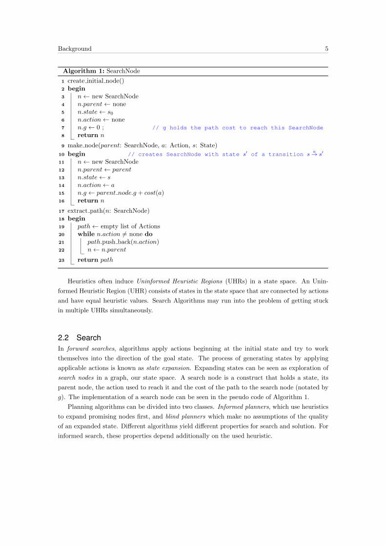
Algorithm 1: SearchNode

1 create initial node()2 begin3 n← new SearchNode4 n.parent← none5 n.state← s0

6 n.action← none7 n.g ← 0 ; // g holds the path cost to reach this SearchNode

8 return n

9 make node(parent: SearchNode, a: Action, s: State)

10 begin // creates SearchNode with state s′ of a transition sa→ s′

11 n← new SearchNode12 n.parent← parent13 n.state← s14 n.action← a15 n.g ← parent node.g + cost(a)16 return n

17 extract path(n: SearchNode)18 begin19 path← empty list of Actions20 while n.action 6= none do21 path.push back(n.action)22 n← n.parent

23 return path

Heuristics often induce Uninformed Heuristic Regions (UHRs) in a state space. An Unin-

formed Heuristic Region (UHR) consists of states in the state space that are connected by actions

and have equal heuristic values. Search Algorithms may run into the problem of getting stuck

in multiple UHRs simultaneously.

2.2 SearchIn forward searches, algorithms apply actions beginning at the initial state and try to work

themselves into the direction of the goal state. The process of generating states by applying

applicable actions is known as state expansion. Expanding states can be seen as exploration of

search nodes in a graph, our state space. A search node is a construct that holds a state, its

parent node, the action used to reach it and the cost of the path to the search node (notated by

g). The implementation of a search node can be seen in the pseudo code of Algorithm 1.

Planning algorithms can be divided into two classes. Informed planners, which use heuristics

to expand promising nodes first, and blind planners which make no assumptions of the quality

of an expanded state. Different algorithms yield different properties for search and solution. For

informed search, these properties depend additionally on the used heuristic.

Background 6

Algorithm 2: Greedy Best-First Search (GBFS)

Input : Π: Planning Taskh: heuristic

Result: π: solution or unsolvable1 open← FIFO priority queue of SearchNodes ordered by h2 closed← empty set of States3 if h(s0) <∞ then4 open.insert(create initial node() )

5 while open is not empty do6 node← open.pop min()7 if node.state ∈ closed then8 continue

9 closed.insert(node.state)10 if G ⊆ node.state then11 return extract path(node) // Goal found

12 foreach 〈a, s′〉 with node.statea→ s′ do // Expand node

13 if h(s′) ≤ ∞ then14 n′ ← make node(node, a, s′)15 open.insert(n′)

16 return unsolvable

Definition 6 (Complete, Semi-Complete, Sound, Satisficing, Optimal)

A search algorithm is:

• Complete, if it finds a solution in case one exists. If there exists no solution the algorithm

will report this.

• Semi-Complete, if it returns a solution in case one exists. In the case of no existing solution

the algorithm may not terminate.

• Sound, if anytime it returns a result, the result is correct.

• Satisficing1, if plans are found without violating any constraints on time, resources and

quality of the solution.

• Optimal, if returned solutions have optimal i.e shortest paths.

2.2.1 Greedy Best First Search (GBFS)Greedy Best-First Search (GBFS) is a class of informed algorithms which expands nodes in order

of their heuristic value. GBFS is a satisficing method and is shown in Algorithm 2.

1 The term satisficing was introduced by Simon (1965) as the combination of satisfy and suffice.

Background 7

s0: 10

s1: 6 s2: 6

s3: 6 s4: 6 s5: 6 s6: 6 s7: 6

s8: 6 s9: 6 s10: 6 s11: 6 s12: 6 s13: 6 s14: 6 s15: 6 s16: 6

s17: 6

gUHR1 UHR2

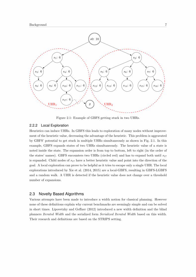
Figure 2.1: Example of GBFS getting stuck in two UHRs.

2.2.2 Local ExplorationHeuristics can induce UHRs. In GBFS this leads to exploration of many nodes without improve-

ment of the heuristic value, decreasing the advantage of the heuristic. This problem is aggravated

by GBFS’ potential to get stuck in multiple UHRs simultaneously as shown in Fig. 2.1. In this

example, GBFS expands states of two UHRs simultaneously. The heuristic value of a state is

noted inside the state. The expansion order is from top to bottom, left to right (in the order of

the states’ names). GBFS encounters two UHRs (circled red) and has to expand both until s17

is expanded. Child nodes of s17 have a better heuristic value and point into the direction of the

goal. A local exploration can prove to be helpful as it tries to escape only a single UHR. The local

explorations introduced by Xie et al. (2014, 2015) are a local-GBFS, resulting in GBFS-LGBFS

and a random walk. A UHR is detected if the heuristic value does not change over a threshold

number of expansions.

2.3 Novelty Based AlgorithmsVarious attempts have been made to introduce a width notion for classical planning. However

none of these definitions explain why current benchmarks are seemingly simple and can be solved

in short times. Lipovetzky and Geffner (2012) introduced a new width definition and the blind

planners Iterated Width and the serialized form Serialized Iterated Width based on this width.

Their research and definitions are based on the STRIPS setting.

Background 8

2.3.1 Iterated Width (IW)Lipovetzky and Geffner (2012) show empirically that the width of many existing domains is bound

and low when goals are restricted to single atoms. A classical planning problem is solvable in

time exponential to its width. The Iterated Width (IW) algorithm tries to take advantage of

these two findings. IW is a blind search algorithm, implementing a pruned breadth-first search.

The pruning is based on the novelty of a state. The novelty of a state in the STRIPS setting is

defined as:

Definition 7 (Novelty)

Let Π = 〈V,O, I,G〉 be a STRIPS planning task.

Let Ti ⊆ P(V ) which is created iteratively during the search as:

• T0 = {∅}

• Ti+1 = Ti ∪ P(si+1),

where si+1 is the (i+ 1)-th expanded state and P(si+1) produces the power set of si+1.

The novelty of si+1 is:

nov(si+1) =

|V |+ 1 if P(si+1) \ Ti = ∅

mint∈P(si+1)\Ti

|t| otherwise.(2.3)

In other words, the novelty of a state si+1 is the size of the smallest subset of si+1 that is

not contained in Ti, where Ti contains all power sets of already encountered states.

The Iterated Width algorithm uses the novelty to prune the search space. In the first iteration

only states with novelty 1 are expanded. These are states where atoms are true that have never

been true before in the search. If the first iteration finds no solution, the next iteration examines

variable sets of size 2. All pairs of true atoms are checked whether this combination has already

been encountered in the iteration. IW can be seen as iterative calls to IW(i), where i denotes

the size of examined variable sets. We call i the novelty-bound. The concept for IW is shown in

Fig. 2.2. The pseudo code for IW is given in Algorithm 3 and Algorithm 4 shows IW(i). IW is

sound and complete. For a problem of width w, IW(w) finds optimal solutions. However IW is

not optimal since a solution can be found in an iteration smaller than its actual width2.

2 Lipovetzky and Geffner (2012) provide a simple example with a goal G of width 2:

• Initial State: {p1, q1}• Actions (without delete effects):

ai : pi → pi+1 and bi : qi → qi+1 | i ∈ {1, . . . 5},a6 : p6 → G,c : {p3, q3} → G

• Goal State: G

IW achieves goal G in a path of size 6, with IW(1) by applying a1, . . . a6. IW(2) returns the optimal path ofsize 5 by applying the action c. IW(1) is unable to apply action c since it prunes states with pairs such as{p2, q3} and {p3, q2} because each variable was true before in the search.

Background 9

s0 g

IW(1)

IW(2)

IW(3)

Figure 2.2: Concept of IW: Novelty-bound is increased in each iteration until the goal can bereached.

Algorithm 3: Iterated Width (IW)

Input : Π: Planning TaskResult: π: solution or unsolvable

1 foreach i ∈ { 1, . . . , number of variables in Π} do2 solution← IW(i) // call IW(i)

3 if solution 6= unsolvable then4 return solution

5 if not IW(i).states pruned then/* If IW(i) pruned no states, IW is in a dead-end */

6 return unsolvable

7 return unsolvable

The line 5 of Algorithm 3 makes sure that IW(i) is not unnecessarily invoked. If IW(i)

does not find a solution and has not pruned any states, IW is stuck in a dead end and returns

unsolvable.

2.3.2 Serialized Iterated Width (SIW)Lipovetzky and Geffner (2012) show empirically that the width of common benchmark problems

is bound and low if the goal is reduced to a single atom of the goal. IW is able to solve these

reduced problems in time exponential to their width.

The problem is however not solved by reaching only one atom of the goal. But these findings

motivate the introduction of the Serialized Iterated Width (SIW) algorithm. SIW uses IW to

automatically split the problem into smaller problems of single atom goals. This is done by

starting IW until one single atom of the goal is reached. IW is then started from this state and

tries to add a second atom of the goal state, and so on. SIW calls IW to iteratively construct

the solution out of single atoms that are part of the goal. It is important to note that the single

atoms reached by IW have to be consistent. Meaning, they do not need to be undone to find a

solution.

Background 10

Algorithm 4: IW(i)

Input : Π: Planning Taski: novelty-bound N 6=0

Result: π: solution or unsolvable with width i1 open← FIFO priority queue of SearchNodes ordered by g2 open.insert(create initial node())3 states pruned← false4 while open is not empty do5 node← open.pop min()6 if G ⊆ node.state then7 return extract path(node) // Goal found

8 foreach 〈a, s′〉 with node.statea→ s′ do

9 n′ ← make node(node, a, s′)10 if novelty(n′.state) > i then // Prune by Novelty

11 states pruned← true12 else13 open.insert(n′)


In the STRIPS settings SIW is defined as:

Definition 8 (Serialized Iterated Width (SIW))

Serialized Iterated Width (SIW) over a STRIPS planning task Π = 〈V,O, I,G〉 consists of a

sequence of calls to IW over the problems Πk = 〈V,O, Ik, Gk〉, k = 1, . . . ,|G|, where:

• I1 = I

• Gk is the first consistent set of atoms achieved from Ik, such that Gk−1 ⊂ Gk ⊆ G and

|Gk| = k;G0 = ∅

• Ik+1 represents the state where Gk is achieved, 1 < k < |G|.

The states containing Gk are called subgoals.

Definition 9 (Subgoal)

Given a STRIPS planning task Π with a set of propositional goal variables G, a subgoal is a state

s which shares variables of the goal G, s ∩G 6= ∅. The size of the subgoal is given by |s ∩G|.

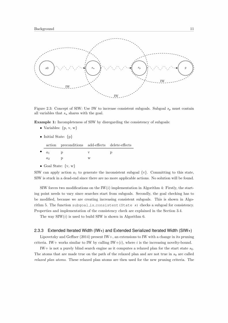
The concept of SIW is displayed in Fig. 2.3. IW is used to reach subgoals and paths between

them. The subgoals are su and sp. The subgoal sp has to contain the previously found subgoal

su and increase it. Additionally the subgoals have to be consistent.

SIW commits to subgoals. If the consistency property does not hold, SIW can commit to a

dead end state, rendering SIW incomplete as shown in Example 1.

Background 11

s0 su sp g

IW

IW

IW

Figure 2.3: Concept of SIW: Use IW to increase consistent subgoals. Subgoal sp must containall variables that su shares with the goal.

Example 1: Incompleteness of SIW by disregarding the consistency of subgoals:

• Variables: {p, v, w}

• Initial State: {p}

•action preconditions add-effects delete-effects

a1 p v p

a2 p w

• Goal State: {v, w}SIW can apply action a1 to generate the inconsistent subgoal {v}. Committing to this state,

SIW is stuck in a dead-end since there are no more applicable actions. No solution will be found.

SIW forces two modifications on the IW(i) implementation in Algorithm 4: Firstly, the start-

ing point needs to vary since searches start from subgoals. Secondly, the goal checking has to

be modified, because we are creating increasing consistent subgoals. This is shown in Algo-

rithm 5. The function subgoal is consistent(State s) checks a subgoal for consistency.

Properties and implementation of the consistency check are explained in the Section 3.4.

The way SIW(i) is used to build SIW is shown in Algorithm 6.

2.3.3 Extended Iterated Width (IW+) and Extended Serialized Iterated Width (SIW+)Lipovetzky and Geffner (2014) present IW+, an extensions to IW with a change in its pruning

criteria. IW+ works similar to IW by calling IW+(i), where i is the increasing novelty-bound.

IW+ is not a purely blind search engine as it computes a relaxed plan for the start state s0.

The atoms that are made true on the path of the relaxed plan and are not true in s0 are called

relaxed plan atoms. These relaxed plan atoms are then used for the new pruning criteria. The

Background 12

Algorithm 5: SIW(i)


start node : SearchNodeResult: sub goal : SearchNode, new consistently increased subgoal or none

states pruned : boolean indicating if states were pruned due to their novelty1 open← FIFO priority queue of SearchNodes ordered by g2 open.insert(start node)3 states pruned← false4 starts goal variables← start node.state ∩G5 while open is not empty do6 node← open.pop min()7 if G ⊆ node.state then8 return 〈node, states pruned〉 // Goal found

9 node goal variables← node.state ∩G10 if starts goal variables ( nodes goal variables then

/* The new subgoal needs to contain the previous subgoal and

increase in size */

11 if subgoal is consistent(node.state) then12 return 〈node, states pruned〉

13 foreach 〈a, s′〉 with node.statea→ s′ do // Similar to IW(i)

14 n′ ← make node(node, a, s′)15 if novelty(n′.state) > i then // Prune by Novelty


19 return 〈none, states pruned〉

new pruning criteria of a search node s considers an extended tuple 〈t,m〉, where t is a set of

atoms of s and m is the number of relaxed plan atoms that were made true on the path reaching

s. For a search node s not to be pruned in IW+(i) it must be the first node of the search to

make an extended tuple 〈t,m〉 true where the number of atoms in t is at most i.

One can visualize the new novelty check as multiple layers of autonomous novelty checks.

The number of reached relaxed plan atoms (m) is the layer in which the state will be checked

for its novelty.

IW+(i) is fundamentally different from IW in that a state can be expanded multiple times.

An example for this behaviour is shown in Fig. 2.4. This example shows a small part of a

state space and the expansion order of IW(1) and IW+(1). A node represents a state and the

variable that are true in that state. The arrows in the state space represent applicable actions

and numbers mark the order they are applied in the search. IW(1) starts by expanding s0 and

s1. By expanding s1 the state s4 gets pruned, since both atoms have already been encountered.

IW+(1) expands these states differently. Lets assume the facts of the relaxed plan consists only

of the variable “c”. By expanding s1 the state s4 gets pruned for now. The search continues

Background 13

Algorithm 6: Serialized Iterated Width (SIW)

Input : Π: Planning TaskResult: π: solution or FAILED

1 i← 1 // novelty bound

2 start node← create initial node()3 while i ≤ number of variables in Π do4 〈end node, states pruned〉 ← SIW (Π, i, start node) // calling SIW(i)

5 if end node is none then// SIW(i) did not find a bigger consistent subgoal.

6 if not states pruned then7 return FAILED

8 i← i+ 1

9 else// SIW(i) did find a bigger consistent subgoal.

10 if G ⊆ end node.state then// SIW(i) found a solution

11 return extract path(end node)

12 else// Start next SIW(i) from new subgoal, with a i of 1

13 start node← end node14 i← 1

15 return FAILED

with the state s2. By expanding s2 we generate the state s3. This state makes one atom of the

relaxed plan atoms true and is checked for its novelty on the layer m = 1. On this layer the atom

“a” has not been seen and therefore s1 gets expanded a second time. The second expansion of

s1 does not prune s4 because the atom “i” is new on the layer m = 1. Algorithm 7 shows the

implementation of IW+(i).

SIW+ works similar to SIW, but uses IW+ instead of IW to serialize the problem.

Background 14

s0: i

s1: a

s2: b

s3: c

s4: a, i

g: p, c

(a) State Space

s0: i

s1: a

s2: b

s3: c

s4: a, i

1

23

(b) IW(1) expansion order

s0: i

s1: a

s2: b

s3: c

s4: a, i

1, m: 0

2, m: 0

3, m: 1

4, m: 1

5, m: 1

6, m: 1

(c) IW+(1) expansion order.

Figure 2.4: (a) displays states by their names and atoms that are true in them. Arrows representapplicable actions between states. (b) shows the expansion order of IW(1). (c) shows theexpansion order of IW+(1) if the relaxed plan consist only of the atom “c”.

Background 15

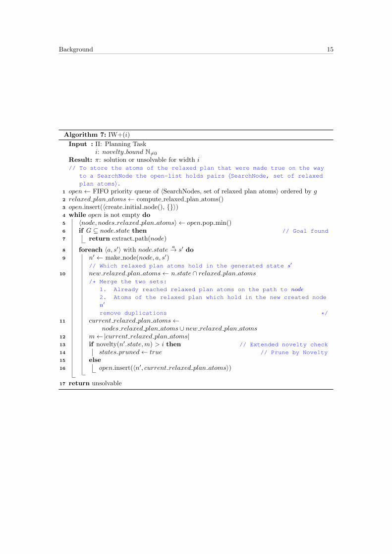
Algorithm 7: IW+(i)

Input : Π: Planning Taski: novelty bound N 6=0

Result: π: solution or unsolvable for width i// To store the atoms of the relaxed plan that were made true on the way

to a SearchNode the open-list holds pairs 〈SearchNode, set of relaxed

plan atoms〉.1 open← FIFO priority queue of 〈SearchNodes, set of relaxed plan atoms〉 ordered by g2 relaxed plan atoms← compute relaxed plan atoms()3 open.insert(〈create initial node(), {}〉)4 while open is not empty do5 〈node, nodes relaxed plan atoms〉 ← open.pop min()6 if G ⊆ node.state then // Goal found

7 return extract path(node)


9 n′ ← make node(node, a, s′)// Which relaxed plan atoms hold in the generated state s′

10 new relaxed plan atoms← n.state ∩ relaxed plan atoms/* Merge the two sets:

1. Already reached relaxed plan atoms on the path to node

2. Atoms of the relaxed plan which hold in the new created node

n′

remove duplications */

11 current relaxed plan atoms←nodes relaxed plan atoms ∪ new relaxed plan atoms

12 m←|current relaxed plan atoms|13 if novelty(n′.state,m) > i then // Extended novelty check

14 states pruned← true // Prune by Novelty

15 else16 open.insert(〈n′, current relaxed plan atoms〉)


3Implementation

This chapter introduces the Fast Downward Planning System (FD) in which the combination of

heuristic and novelty guided search will be implemented. The Fast Downward Planning System

uses a Multi-Value Planning Task instead of STRIPS, such that previously defined ideas and

definitions have to be adapted. After the adaption we present data structures and their use in

the implementations of FD.

3.1 Fast Downward (FD)The Fast Downward Planning System (FD) was introduced by Helmert (2006). It is an open-

source3 framework written in C++. Fast Downward uses a Multi-Value Planning Task (MPT)

which is introduced in Definition 10. The MPT of FD is slightly more sophisticated as it addi-

tionally supports axioms.

The Fast Downward Planning System supports multiple search algorithms and heuristics and

enables users to easily combine them over a command line interface.

FD is capable of using improvements such as combining multiple heuristics introduced by

Roger and Helmert (2010), use of helpful actions or preferred operators introduced by Hoffmann

and Nebel (2001) and deferred evaluation introduced by Richter and Helmert (2009). FD enables

researchers to implement their ideas and integrate them as plug-ins into the Fast Downward

Planning System.

Definition 10 (Multi-Valued Planning Task (MPT))

A multi-valued planning task (MPT) is a 5-tuple Π = 〈V, dom,O, I,G, 〉 where

• V is a finite set of state variables.

3 http://www.fast-downward.org

Implementation 17

• dom is a function assigning every variable v ∈ V a non-empty domain dom(v).

We call a variable-value assignment 〈var, value〉, where var ∈ V and value ∈ dom(variable)

a fact.

A partial (variable) assignment or partial state is a set of consistent facts.

A state s is a set of consistent facts, where |s| = |V |.

• O is a finite set of operators. Each operator o ∈ O is a pair of 〈pre, effect〉, where pre are

preconditions in the form of a partial state and effect is a function assigning a portion of

variables new values of their domain.

• I is a state over V called the initial state.

• G is a partial state called the goal.

A state that shares facts of the goal is called a subgoal.

A special feature of FD is the translation of a STRIPS problem into an MPT. This is done by

identifying groups of variables for which only one can be true at all times. A simple example for

such a group of variables can be a truck’s position in a logistics problem: A truck has to deliver

multiple packets to several locations. The STRIPS setting models this by introducing a variable

for each location the truck can be at. FD recognizes that the truck can only be at one place at

a time through an invariant synthesis. FD then introduces a multi-value variable for the truck

with the locations as its domain.

3.2 Adaptions for the MPT SettingTo implement the relevant algorithms in the MPT setting the novelty definition of the STRIPS

has to be adapted. The novelty Definition 7 tells us to look for new sets of atoms. This definition

can directly be applied to an MPT planning task by looking for new sets of facts. The power set

produces now sets of facts instead of sets of atoms. The novelty is then the smallest set of the

power set which hasn’t been seen before, or |V |+ 1 if all these sets are already known.

Even though we use the same novelty definition as in the STRIPS setting, IW is not equal

in the STRIPS and MPT setting. An example showing the difference is given in the following

proposition:

Proposition 1 (Inequality of IW in STRIPS and MPT)

FD creates MPT out of STRIPS planning tasks by grouping variables for which only one can be

true at all times. But there is also a possibility that none of those variables is true in a state.

For this situation FD introduces a “none of those” value. This value can make a difference if a

state gets pruned or not. If a state in the MPT contains a “none of those” value for the first

time it wont get pruned. This state could very well be pruned in the STRIPS setting, as setting

variables to false does not generate a new set of true variables.

Implementation 18

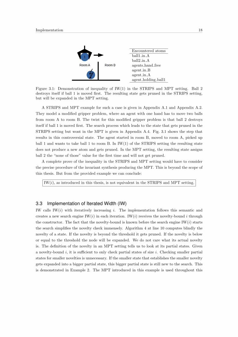
Encountered atomsball1 in Aball2 in Aagents hand freeagent in Bagent in Aagent holding ball1

Figure 3.1: Demonstration of inequality of IW(1) in the STRIPS and MPT setting. Ball 2destroys itself if ball 1 is moved first. The resulting state gets pruned in the STRIPS setting,but will be expanded in the MPT setting.

A STRIPS and MPT example for such a case is given in Appendix A.1 and Appendix A.2.

They model a modified gripper problem, where an agent with one hand has to move two balls

from room A to room B. The twist for this modified gripper problem is that ball 2 destroys

itself if ball 1 is moved first. The search process which leads to the state that gets pruned in the

STRIPS setting but wont in the MPT is given in Appendix A.4. Fig. 3.1 shows the step that

results in this controversial state. The agent started in room B, moved to room A, picked up

ball 1 and wants to take ball 1 to room B. In IW(1) of the STRIPS setting the resulting state

does not produce a new atom and gets pruned. In the MPT setting, the resulting state assigns

ball 2 the “none of those” value for the first time and will not get pruned.

A complete prove of the inequality in the STRIPS and MPT setting would have to consider

the precise procedure of the invariant synthesis producing the MPT. This is beyond the scope of

this thesis. But from the provided example we can conclude:

IW(i), as introduced in this thesis, is not equivalent in the STRIPS and MPT setting.

3.3 Implementation of Iterated Width (IW)IW calls IW(i) with iteratively increasing i. The implementation follows this semantic and

creates a new search engine IW(i) in each iteration. IW(i) receives the novelty-bound i through

the constructor. The fact that the novelty-bound is known before the search engine IW(i) starts

the search simplifies the novelty check immensely. Algorithm 4 at line 10 computes blindly the

novelty of a state. If the novelty is beyond the threshold it gets pruned. If the novelty is below

or equal to the threshold the node will be expanded. We do not care what its actual novelty

is. The definition of the novelty in an MPT setting tells us to look at its partial states. Given

a novelty-bound i, it is sufficient to only check partial states of size i. Checking smaller partial

states for smaller novelties is unnecessary. If the smaller state that establishes the smaller novelty

gets expanded into a bigger partial state, this bigger partial state is still new to the search. This

is demonstrated in Example 2. The MPT introduced in this example is used throughout this

Implementation 19

chapter to demonstrate operational and conceptual behaviour of implementations.

Example 2: To check whether the novelty of a state is 2 or below it is sufficient to only check

partial states of size 2.

Variable Domains:∣∣∣ 2 4 6 5∣∣∣

State generation order:

s0 :∣∣∣ 0 0 0 0

∣∣∣s1 :

∣∣∣ 1 0 0 0∣∣∣

The MPT has 4 variables. The variable domains are given on the

left. The first entry means that the first variable can only take on two

different values: 0 or 1. The second variable can take on 4 different

values . . . .

The search first generates the initial node s0. The value of each

variable in s0 is 0. The second generated state in the search is s1.

s1 has a novelty of 1 due to its first variable with the never before

seen value of 1. However, we are only interested if the novelty is 2 or

below. Every partial state of size 2 containing the first variable lets

us conclude that the novelty of s1 is in fact 2 or below. The actual

novelty is irrelevant.

Only checking whether a state’s novelty is below or equal a threshold is not enough in order

for IW to work. All encountered partial states of given size have to be stored in a data structure.

This data structure should be optimized for lookups and insertions.

The chosen implementation consists of multiple coherent arrays: vectors of the C++ stan-

dard library. At the beginning all subsets of size novelty-bound are created and stored in a

vector<int>. Each int in the array points at a variable of a state. The subsets are used to

create the partial states of size novelty-bound from a given state.

Every possible partial state of size novelty-bound gets its place in a vector<bool> called

lookup. The mapping between a partial state and its position in lookup is done with the help

of another vector<int> called offsets. offsets is filled during creation of the subsets

and provides a jumping point into lookup. From this jumping point we need to determine the

position of the partial state compared to its other possible assignments. An example of this data

structure and its initialization is displayed in Example 3. Example 4 demonstrates the use of

the data structure to determine if a partial state has been encountered before in the search. To

check whether a state gets pruned due to its novelty and storing partial states in the process is

shown in Example 5.

Implementation 20

Example 3: Data structure that stores encountered partial states during the search.

variable domains∣∣∣ 2 4 6 5∣∣∣

subsets∣∣∣∣∣∣∣∣∣∣∣∣∣∣∣

0 1

0 2

0 3

1 2

1 3

2 3

∣∣∣∣∣∣∣∣∣∣∣∣∣∣∣

offsets∣∣∣∣∣∣∣∣∣∣∣∣∣∣∣

0

0 + 2 ∗ 4 = 8

8 + 2 ∗ 6 = 20

20 + 2 ∗ 5 = 30

30 + 4 ∗ 6 = 54

54 + 4 ∗ 5 = 74

∣∣∣∣∣∣∣∣∣∣∣∣∣∣∣

lookup∣∣∣∣∣∣∣∣∣∣∣∣∣∣∣∣∣

0

0......

0

0

∣∣∣∣∣∣∣∣∣∣∣∣∣∣∣∣∣

The size of the lookup

is the number of possi-

ble partial states with

size 2:

74 + 6 ∗ 5 = 104

variable domains is the same as in Example 2.

For each subset in subsets a jumping point is computed and stored in offsets. The first

entry of offsets is 0 because indexing of lookup starts with 0. The second entry in offsets

takes the first subset 〈0, 1〉 to compute the jumping point. The subset 〈0, 1〉 points at the first

and second variable. These two variables are able to create 2 ∗ 4 different assignments. The

jumping point for the second subset is therefore 8, placing it after all possible assignments of

the first subset. The next jumping point computes the possible assignments of the second subset

and adds these to the previous jumping point 8 + 2 ∗ 6. The entries in lookup are all initialized

with false or 0 because no partial state has been encountered so far.

Example 4: Checking whether a partial state has been encountered in the search or not.

Given is the initialized data structure of Example 3. The encountered state is s = 〈0, 3, 1, 4〉.The fifth subset of subsets, 〈1, 3〉 produces the partial state 〈3, 4〉 for which we determine if it

has been encountered in the search before.

Determination whether the partial state has been encountered is done by:

• taking the jumping point into lookup of subset 〈1, 3〉 is taken from offsets and is 54.

• computing the position of this partial state compared to other possible assignments. The

first variable of the partial state is 3. Considering that 0 is a valid assignment, there are 3

different assignments of the first variable before the assigned 3. These three assignments can

be combined with the domain size of the last variable: 3∗5 = 15. To these 15 possible assign-

ments there are still an additional 4 before our partial state: 〈〈3, 0〉, 〈3, 1〉, 〈3, 2〉, 〈3, 3〉〉. The

position of this partial state compared to other possible assignments is therefore 15+4 = 19.

• Whether the subset 〈1, 3〉 creating the partial state 〈3, 4〉 has been encountered in the

search before, is stored in the boolean of lookup at the position: 54 + 19.

Example 5: Checking if the novelty is 2 or below and storing all partial states in the process.

Given is the data structure of Example 3. The encountered state is s = 〈0, 3, 1, 4〉. To check

whether the novelty of s is 2 or below we have to iterate over all subsets of the novelty data

Implementation 21

structure. For each subset we then have to get the entry in lookup corresponding to the partial

state created by the subset as shown in Example 4. If the boolean entry in lookup at this

corresponding position is 0 (standing for false), the novelty of s is indeed 2 or below. We then

have to set it to 1 (standing for true) for further checks.

Important is now that we must not break the iteration over the subsets. We have to set all

corresponding entries for all partial states in lookup to true. Breaking this loop would tamper

with later novelty computations, as already encountered partial states would not be recorded.

We chose a vector<int> for subsets because it simplifies the construction of partial states

and requires less memory for small novelty-bounds than a bit-map. The vector offsets is

stored because its values are needed in each novelty check, making this simple lookup faster

than the computation. The vector lookup is then a simple and fast way to check and store

if a partial state has been encountered. lookup may allocate memory for booleans (encoding

partial states) that are not reachable in the MPT and will never be used. These dead spaces are

negligible compared to a map-based implementations and their overheads.

We chose the presented implementation with coherent arrays because it proofed to be faster

than a mapping approach of: subset ↔ set of partial states. Tests of IW on a gripper problem

with 10 balls showed a speedup of 4 by using coherent arrays over the map approach. The

speedup even increases for bigger problems.

The implementation of IW and IW(i) is an adaption from the pseudo code of Algorithm 3

and Algorithm 4 into C++ and the framework of the Fast Downward Planning System.

3.3.1 Improvement: Novelty check with generating operatorOne can take advantage of the fact that nodes are generated by applying an operator. The

operator dictates which variables get new values assigned. In the novelty check we have to only

check the subsets containing these variables. During the initialization of the data structure an

additional vector is created. Each entry of this vector stands for a variable and holds pointers

to the subsets the variable appears in. The novelty check has then to iterate over the subsets

containing a changed variable. With IW on the gripper problem with 10 balls we got a speedup

of 1.1 by this approach.

3.3.2 Improvement: Taking advantage of the Fast Downward Search NodesThe Fast Downward Planning system implements search nodes different than introduced in

this thesis. Per state s there exists at maximum one search node with this state. A search node

with state s has one of the following statuses:

• NEW: No node with state s has been opened before.

• OPEN: A search node with state s already exists and is open.

Implementation 22

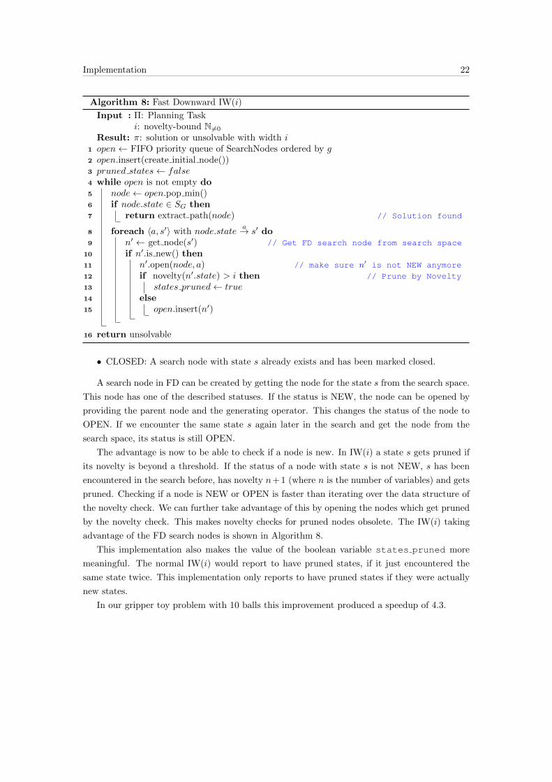
Algorithm 8: Fast Downward IW(i)


Result: π: solution or unsolvable with width i1 open← FIFO priority queue of SearchNodes ordered by g2 open.insert(create initial node())3 pruned states← false4 while open is not empty do5 node← open.pop min()6 if node.state ∈ SG then7 return extract path(node) // Solution found


9 n′ ← get node(s′) // Get FD search node from search space

10 if n′.is new() then11 n′.open(node, a) // make sure n′ is not NEW anymore

12 if novelty(n′.state) > i then // Prune by Novelty



• CLOSED: A search node with state s already exists and has been marked closed.

A search node in FD can be created by getting the node for the state s from the search space.

This node has one of the described statuses. If the status is NEW, the node can be opened by

providing the parent node and the generating operator. This changes the status of the node to

OPEN. If we encounter the same state s again later in the search and get the node from the

search space, its status is still OPEN.

The advantage is now to be able to check if a node is new. In IW(i) a state s gets pruned if

its novelty is beyond a threshold. If the status of a node with state s is not NEW, s has been

encountered in the search before, has novelty n+ 1 (where n is the number of variables) and gets

pruned. Checking if a node is NEW or OPEN is faster than iterating over the data structure of

the novelty check. We can further take advantage of this by opening the nodes which get pruned

by the novelty check. This makes novelty checks for pruned nodes obsolete. The IW(i) taking

advantage of the FD search nodes is shown in Algorithm 8.

This implementation also makes the value of the boolean variable states pruned more

meaningful. The normal IW(i) would report to have pruned states, if it just encountered the

same state twice. This implementation only reports to have pruned states if they were actually

new states.

In our gripper toy problem with 10 balls this improvement produced a speedup of 4.3.

Implementation 23

3.4 Serialized Iterated Width (SIW)SIW uses IW to construct subgoals of increasing size until a solution is found. The SIW(i)

implementation in the Fast Downward planning system inherits from the IW(i) implementation.

The difference lies in the condition when SIW(i) stops. For the Iterated Width algorithm, IW(i)

needs to find the solution. SIW(i) needs to find a subgoal. The conditions on the subgoal are:

1. The subgoal needs to extend the previous subgoal, i.e the subgoal size must increase and

the previous subgoal must be contained in the new one.

2. The subgoal needs to be consistent: it does not have to be undone to find a solution.

Checking the first condition is simple. But checking a subgoal for consistency is equivalent

to solving the problem beginning at the subgoal. We weaken the consistency condition by using

a safe heuristic for the subgoal candidate as proposed by Lipovetzky and Geffner (2012). A

safe heuristic has the property that if h(s) =∞ then there exists no solution for state s. Before

calculating the heuristic value, operators that change the assignment of the subgoal are removed.

We then check if the heuristic value is infinite or not. This check is weaker than the introduced

consistency because of the safe heuristic. If this modified heuristic value tells us the distance

from the subgoal to the goal is infinite, we know that the subgoal is not consistent. However,

there might be cases where the heuristic value is smaller than infinite, but there still exists no

path to the goal. Considering this weak consistency test we do not prune states which change

already reached subgoals in SIW. Due to the weak consistency check SIW might be incomplete

if there are actual dead-ends in the problem definition.

In the Fast Downward Planning System this weak consistency uses a modified relaxation

heuristic which allows disabling operators and checking relaxed reachability.

3.5 IW+ and SIW+To obtain IW+/SIW+, the implementation of IW and SIW require a few changes:

• It is required to know how many facts of the relaxed plan were made true on the path to

a search node. As shown in Algorithm 7, the open list holds a tuple. In the MPT setting

this tuple contains a search node as well as a set of facts. This set of facts contains those

facts of the relaxed plan that were encountered on the path to the node. It is not sufficient

to just keep track of the number of relaxed plan facts a node encountered on its path. This

is insufficient because a new state might make relaxed plan facts true, which were already

encountered on the path.

These relaxed plan facts are stored as a vector of booleans in the open list. Each position

of this vector stands for a fact of the relaxed plan. The open list is no longer a State Open

List implemented by FD, but a priority queue of the C++ standard library.

Implementation 24

• The novelty check needs to be adapted to deal with the extended tuple 〈t,m〉. The boolean

vector lookup needs to have multiple layers. The number of layers is the size of the relaxed

plan facts + 1. The additional layer is for search nodes, which do not make any relaxed

plan facts true on their path.

• The improvement of the novelty check with the generating operator as described in Sec-

tion 3.3.1 has to be disabled. This is the case because the layers of the novelty check are

independent. If a state is known on one layer it is not sufficient to check only the changed

subsets on another layer. Eg: state 〈5, 3, 2〉 is known on layer 1 (it made 1 fact of the

relaxed plan true on its path). If an operator changes the first entry to 1 and makes and

additional fact of the relaxed plan true the novelty will be checked on layer 2. On this layer

the whole state might be new and all its partial states have to be added in the layer.

• In IW+ and SIW+, a once pruned state might be expanded later in the search if it made

more relaxed plan facts true on its path. Due to this property the improvement of closing

nodes and checking nodes whether they are new as described in the Section 3.3.2 has to be

disabled as well.

4Iterated Width and Serialized Iterated Width on

Uninformed Heuristic Regions

The basic idea of this thesis is to mix up the search when GBFS gets stuck in UHRs. The new

approach expands states only if they are novel enough in order to try to escape UHRs. The

intuition behind this idea is that the heuristic might assess nodes that are pretty similar with

equal heuristic values. By disregarding the heuristic and expanding nodes which are novel to the

search we hope to escape UHRs quicker and find solutions faster.

One precondition to implement this idea is the recognition of UHRs during the GBFS search.

This is done by counting the number of consecutively expanded states with equal heuristic values

as proposed by Xie et al. (2014). Once a given threshold is reached we are stuck in UHRs.

This section describes two approaches to combine GBFS with IW and SIW when GBFS

encounters UHRs.

4.1 Chain of GBFS and IW/SIWThe first approach to combine GBFS with IW/SIW is similar to SIW. But instead of a

subgoal, GBFS commits to a state in an UHR. This approach is shown in Fig. 4.1. GBFS counts

the number of consecutive expanded states with the same heuristic value. If this number reaches

a threshold, a local search is started from that state. The local search can be IW, IW+, SIW

or SIW+. The difference in implementation is that GBFS has to count how many states it

expanded with stationary heuristic value. The only difference in the local searches affects the

goal checking. Each state that gets expanded by the local search needs to be evaluated by the

heuristic. If a state improved the heuristic value, the local search escaped the UHR and a new

GBFS is started from that state.

This approach has multiple short comings. The most severe might be that it commits to

states in UHRs. If this quite arbitrarily chosen state is in an enormous UHR or even in a dead-

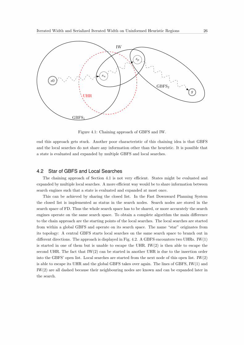
Iterated Width and Serialized Iterated Width on Uninformed Heuristic Regions 26

s0

su

GBFS1

UHR

IW

sp

g

GBFS2

Figure 4.1: Chaining approach of GBFS and IW.

end this approach gets stuck. Another poor characteristic of this chaining idea is that GBFS

and the local searches do not share any information other than the heuristic. It is possible that

a state is evaluated and expanded by multiple GBFS and local searches.

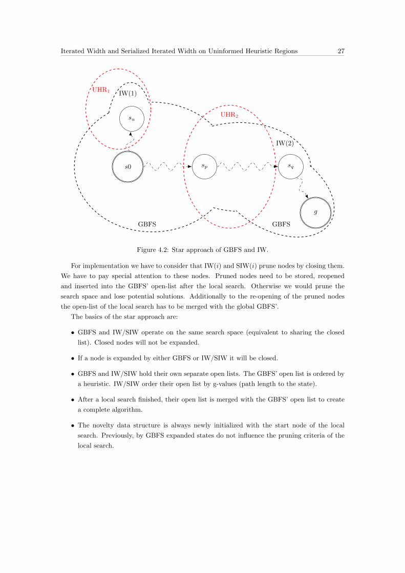
4.2 Star of GBFS and Local SearchesThe chaining approach of Section 4.1 is not very efficient. States might be evaluated and

expanded by multiple local searches. A more efficient way would be to share information between

search engines such that a state is evaluated and expanded at most once.

This can be achieved by sharing the closed list. In the Fast Downward Planning System

the closed list is implemented as status in the search nodes. Search nodes are stored in the

search space of FD. Thus the whole search space has to be shared, or more accurately the search

engines operate on the same search space. To obtain a complete algorithm the main difference

to the chain approach are the starting points of the local searches. The local searches are started

from within a global GBFS and operate on its search space. The name “star” originates from

its topology: A central GBFS starts local searches on the same search space to branch out in

different directions. The approach is displayed in Fig. 4.2. A GBFS encounters two UHRs. IW(1)

is started in one of them but is unable to escape the UHR. IW(2) is then able to escape the

second UHR. The fact that IW(2) can be started in another UHR is due to the insertion order

into the GBFS’ open list. Local searches are started from the next node of this open list. IW(2)

is able to escape its UHR and the global GBFS takes over again. The lines of GBFS, IW(1) and

IW(2) are all dashed because their neighbouring nodes are known and can be expanded later in

the search.


s0

su

UHR1 IW(1)

UHR2

sp

IW(2)

sq

g

GBFS GBFS

Figure 4.2: Star approach of GBFS and IW.

For implementation we have to consider that IW(i) and SIW(i) prune nodes by closing them.

We have to pay special attention to these nodes. Pruned nodes need to be stored, reopened

and inserted into the GBFS’ open-list after the local search. Otherwise we would prune the

search space and lose potential solutions. Additionally to the re-opening of the pruned nodes

the open-list of the local search has to be merged with the global GBFS’.

The basics of the star approach are:

• GBFS and IW/SIW operate on the same search space (equivalent to sharing the closed

list). Closed nodes will not be expanded.

• If a node is expanded by either GBFS or IW/SIW it will be closed.

• GBFS and IW/SIW hold their own separate open lists. The GBFS’ open list is ordered by

a heuristic. IW/SIW order their open list by g-values (path length to the state).

• After a local search finished, their open list is merged with the GBFS’ open list to create

a complete algorithm.

• The novelty data structure is always newly initialized with the start node of the local

search. Previously, by GBFS expanded states do not influence the pruning criteria of the

local search.


• IW/SIW prune nodes by closing them. These nodes are stored in an ignored list. After

IW/SIW ended, their ignored list is merged into the GBFS’ open list and said nodes

statuses are set to open (equivalent to removing said nodes from a closed list).

Using IW+/SIW+ as local search is more complicated. IW+ and SIW+ prune states based

on the extended novelty criteria. This may lead to multiple expansions of the same state, if

the number of relaxed plan facts of its path increased since the last visit. We do not want to

expand closed nodes but are not able to close nodes due to the property that a state might need

to be expanded multiple times in IW+. Thus we have to store the expanded nodes of IW+ and

SIW+ in a separate closed set. The ignored list is used to store nodes which were pruned by

their novelty. Since a node of ignored can still be expanded later we have to make sure that

closed and ignored are mutually exclusive by removing said nodes from ignored. At the

end of the local search the ignored list is inserted into the GBFS’ open list. The states stored in

the separate closed list have to be closed in the search space for good.

If a local search fails to escape the plateau, the global GBFS resets its UHR detection and

continues with its heuristic search.

This approach is complete, since it does not prune any nodes. All nodes that would be

pruned by a local search are inserted into the GBFS open-list. Thus, given enough time, the

whole search space can be expanded.

5Experiments and Results

This section presents conducted experiments and their results. We start by comparing SIW and

SIW+ in the STRIPS and MPT setting. We then evaluate two heuristic based GBFS approaches

and compare them to our planners that combine heuristic and novelty based searches.

5.1 SetupAll benchmarks were run on a cluster of Intelr Xeonr processors running CentOS 6.5 at

2.2 GHz. Each task was executed on a single processor core with a time limit of 30 minutes

and a memory limit of 2 GB. The Fast Downward was compiled with GCC 4.8.4 for a 32 bit

architecture.

The benchmarks consist of 46 domains resulting in a total of 1456 satisficing planning prob-

lems.

5.2 Baseline AlgorithmsFirst we compared SIW and SIW+ of the STRIPS setting4 to our implementation in the

MPT setting. We then proceeded to evaluate the default GBFS of FD and compared it to the

GBFS that detects UHRs. Since the only difference is a counter in one of them, there was no

observable difference. For further experiments we recall with GBFS the one detecting UHRs.

We then proceeded to compare the GBFS with a GBFS using preferred operators, GBFSpreferred.

This modified GBFS produces in each state a set of helpful actions as proposed by Hoffmann

and Nebel (2001). In the MPT helpful actions are called preferred operators. Operators that

appear in the relaxed plan of the state and are applicable in it are preferred operators of said

state. The intuition is that a successor state is more promising if it is generated by a preferred

4 Source code for SIWSTRIPS and SIW+STRIPS available under: https://github.com/miquelramirez/LAPKT-public.git. Tested on committed version: 6d5ce1c of May 16, 2016.

Experiments and Results 30

Table 5.1: Coverage of the baseline algorithms SIW and SIW+ in the STRIPS and MPT setting.SIWSTRIPS and SIW+STRIPS operate on the STRIPS setting. SIW/SIW+ are the implementa-tions embedded in the MPT of the Fast Downward.

SIWSTRIPS SIW SIW+STRIPS SIW+

1075 1040 1167 1162

operator. FD implements this preference with two separate open lists. One containing all suc-

cessors and one containing exclusively states that are produced by preferred operator. The next

state to be expanded by GBFSpreferred is alternatingly taken from one of these two open lists.

This approach proved to be helpful in domains where heuristic guidance is weak and a lot of

time is spent exploring UHRs.

If not mentioned otherwise the heuristic used with GBFS and the heuristic that produces

preferred operators is the ff -heuristic of Hoffmann and Nebel (2001).

A detailed table with the baseline results can be found in Appendix A.5.

5.2.1 SIW and SIW+ in the STRIPS and MPT settingTable 5.1 compares the SIW and SIW+ in the STRIPS and MPT setting. In this experiment we

observe that SIW+ outperforms SIW substantially in both settings. But the coverages vary in

the different settings. Our implementation of SIW and SIW+ is not quite able to solve as many

problems as the implementation of Lipovetzky and Geffner (2012). We suspect three reasons:

• Differing operator orders: The order of introducing a state’s children to the search influences

the pruning criteria and therefore the expansion order. For example: SIWSTRIPS is not able

to solve a single instance of the movie domain. These verdicts are reached in mere seconds,

revealing that SIWSTRIPS runs into dead-ends. Our SIW is able to solve all problems of

this domain.

• Checking the novelty in the STRIPS setting can be more efficient: The number of tuples

that need to be checked in a state might be smaller, as shown in Appendix A.3.

• The expansion order in the MPT might be different through the introduction of “none of

those” values as stated by Proposition 1. This can lead to expansion of states that would

be pruned in the STRIPS setting. Pruning less nodes in the MPT setting could explain

why SIW in the MPT setting runs less often into dead ends but more often out of time.

5.2.2 SIW vs GBFSBy comparing SIW and SIW+ to the GBFS in Table 5.2 we observe that GBFSpreferred

performs best. The SIW+ however, is a close runner up. This is somewhat surprising since

SIW+ is almost a blind planner. It would be interesting to implement complete versions of SIW


Table 5.2: Coverage of the baseline algorithms SIW, SIW+ and GBFS.

SIW SIW+ GBFS GBFSpreferred

1040 1162 1075 1171

Table 5.3: Coverage of the chaining approach of GBFS and local searches with different UHRthreshold sizes. The UHR threshold notes the number of steps without improving the heuristicvalue in GBFS after which a local search is started. Red colours indicate high coverage and bluelow coverage.

UHR thresholdLocal Search 10 100 1000 2000 3000 4000 5000 6000 7000IW 922 1016 1067 1092 1102 1100 1100 1100 1100IW+ 1006 1090 1139 1163 1166 1163 1169 1165 1162SIW 984 1075 1122 1147 1148 1147 1146 1150 1142SIW+ 1022 1103 1152 1167 1175 1169 1173 1166 1168

and SIW+. These complete algorithms could backtrack in dead-ends and would not be permitted

to commit to subgoals that lead them into dead ends. This improvement has the potential for

SIW+ to solve 81 more problems in which the planner runs into dead ends. SIW+ might be able

to surpass the performance of GBFSpreferred.

5.3 Chaining ApproachThe results for the chaining approach of Section 4.1 are displayed as heat map in Table 5.3.

This approach has one tunable parameter: the UHR threshold. This threshold determines the

number of expansions without improvement of the heuristic value, after which a local search is

started. Red colours in the table indicate high coverage and blue low coverage. Detailed domain

coverages for the best configurations are given in Appendix A.6.

In these experiments we observed that the performance is highly dependant on the choice

of the UHR threshold parameter. Best performances are reached if a local search is started

somewhere between 2’000 and 5’000 expansions without improvement of the heuristic value. We

explain these high thresholds by the choice of the state from which a local search is started. This

state is chosen quite arbitrarily and might be a terrible choice. If the UHR threshold is low and

we commit early in UHRs, we might pick states in dead ends. By putting off the commitment,

GBFS might fully expand these dead end UHRs, such that the local search then can be started

from within a promising one.

The local searches IW+ and SIW+ which use the extended pruning criteria outperform their

counterparts IW and SIW. SIW+ as local search dominates in all configurations. Even with the

short comings of committing to dead-ends and the possibility of expanding states multiple times,

the best configuration solves more problems than GBFSpreferred (1175 vs. 1171).


Table 5.4: Coverage for different configurations of the star approach. Novelty-Bound is themaximum novelty-bound for local searches to be started with. UHR threshold notes the numberof steps without improving the heuristic value in GBFS after which a local search is started. MaxSteps is the maximum number of expansions a local GBFS is allowed to perform. Red coloursindicate high coverage and blue low coverage.

LocalPlanner

Novelty-Bound

UHR threshold10 50 100 500 1000

IW

1 1157 1151 1161 1144 11402 1139 1136 1151 1152 11613 1105 1112 1115 1133 1150∞ 1059 1075 1086 1108 1126

IW+

1 1251 1236 1232 1222 12192 1209 1214 1209 1205 12063 1178 1187 1195 1200 1200∞ 1149 1171 1183 1189 1201

SIW

1 1149 1158 1161 1156 10712 1139 1156 1149 1146 11403 1100 1135 1131 1139 1141∞ 948 996 1016 1055 1140

SIW+

1 1161 1173 1171 1171 11502 1157 1175 1169 1172 11593 1135 1157 1159 1170 1153∞ 1028 1086 1086 1113 1113

Max Steps

GBFS

10 1109 1110 1110 1110 110250 1126 1128 1124 1117 1106100 1124 1121 1123 1118 1116600 1109 1114 1110 1111 11061000 1105 1109 1117 1104 1098∞ 1044 1048 1052 1053 1057

5.4 Star ApproachThe results for the star approach of Section 4.2 are displayed as heat map in Table 5.4. This

approach has two parameters to tune: The UHR threshold and the range for the novelties. If

the novelty-bound for a local search engine is 3, the first local search engine is started with a

novelty-bound of 1. If it is not able to escape the UHR a second local search is started with a

novelty-bound of 2. The starting point of the second local search is taken from the open list of

the global GBFS. The novelty-bound gives the upper bound for local searches to search with.

We also implemented our own GBFS-LGBFS of Xie et al. (2014). GBFS-LGBFS is implemented

in the star approach. The local search engine is a GBFS that stops if it encounters a state with

better heuristic value or reaches the maximum number of expansions it is allowed to perform

(Max Steps).

We observe an antipodal trend to the results of the chaining approach: Performance is gen-

erally better with smaller UHR threshold sizes. This was somehow expected. In the chaining


approach we run the risk of committing to dead ends. In the star approach we do not commit

to states. Even starting local searches in huge UHRs or dead ends is no threat. The more often

a small local search is started, the bigger the chance of starting it in a state close to the border

of an UHR. If the local search is unsuccessful in escaping the UHR, the global GBFS continues

for a maximum of UHR threshold number of expansions. If this UHR threshold is small, we

increase the chance of starting a local search in a promising position even further. However, we

cannot go too low with the UHR threshold size, since the overhead for initializing the novelty

data structure would be too severe.

GBFS with local GBFS performs better than a single GBFS (1075). Again, starting multiple

small GBFS seems more promising than starting a few big ones. The coverages among all GBFS-

LGBFS are pretty similar. If the number of steps in the local GBFS is not bounded, the positive

effect of using a local GBFS diminishes entirely.

In the results we see again, that the local searches with the extended pruning criteria usually

perform better than their counterparts. Using IW or IW+ as local searches produce better

coverage than their serialized counterparts. This feels somehow natural, since SIW or SIW+ can

locally commit to subgoals which will be the starting point for their subsequent local searches.

Using IW+ as local search performs best. With a novelty-bound of 1 and an UHR threshold

size of 10 it is able to solve 1251 problems; 80 more than GBFSpreferred.

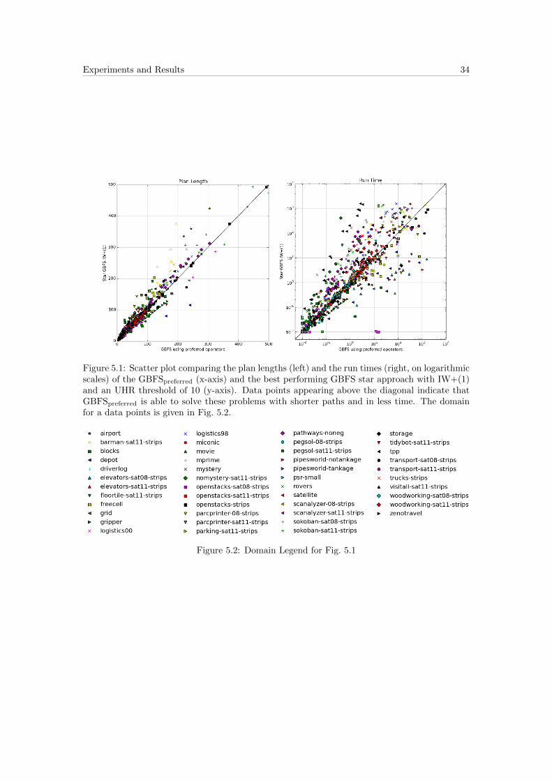
5.5 Comparison of the best planners: GBFSpreferred vs. Star-GBFS-IW+(1)We compare the plan lengths and execution times of the two best planners: GBFSpreferred

and the star approach with IW+ (novelty-bound of 1 and an UHR threshold of 10). A point in

the scatter plot represents two measures: One of the baseline algorithm GBFSpreferred (x-axis)

and one of Star-GBFS-IW+(1) (y-axis). Only problems which both planners were able to solve

are displayed. If the result for a problem is better solved by GBFSpreferred it will appear above

the diagonal. As the figure Fig. 5.1 shows, the GBFSpreferred usually produces shorter paths and

is faster in doing so. This is somehow expected, since we solely try to escape UHRs without

respect to optimality in doing so. Longer paths could then result in more time usage to expand

nodes along these longer paths. These graphs are somehow misleading as they solely show that

GBFSpreferred is faster and finds better solution when both planners are able to solve the problem.

These graphs do not address the number of problems which Star-GBFS-IW+(1) is able to solve

that GBFSpreferred cannot.


Figure 5.1: Scatter plot comparing the plan lengths (left) and the run times (right, on logarithmicscales) of the GBFSpreferred (x-axis) and the best performing GBFS star approach with IW+(1)and an UHR threshold of 10 (y-axis). Data points appearing above the diagonal indicate thatGBFSpreferred is able to solve these problems with shorter paths and in less time. The domainfor a data points is given in Fig. 5.2.

Figure 5.2: Domain Legend for Fig. 5.1

6Conclusion and Future Work

In this thesis we discussed the blind novelty-based search algorithms Iterated Width (IW), Serial

Iterated Width (SIW) and their extensions IW+ and SIW+. We adapted the novelty into the

MPT setting and implemented IW, IW+ and SIW, SIW+ in the Fast Downward Planning

System. We showed that the adaption in the MPT setting induces differences: The MPT may

introduce “none of those” variables. These can lead to expansion of states which would be pruned

in the STRIPS setting.

We then used the novelty based search engines to escape UHRs in GBFS with two approaches:

The first approach is a chain of search engines which share no information. The second approach

shares information of already expanded states between GBFS and local searches. This produces a

complete algorithm with no re-opening of already expanded nodes (IW+ and SIW+ may locally

re-open nodes).

The results show that changing the search approach to escape UHRs can be helpful. By tightly

coupling the heuristic and novelty guided search, we managed to surpass the best performing

GBFS by 80 problems. The increase in coverage however, may go to the expense of run time

and quality of the solutions.

Possible future work includes a complete SIW/SIW+ algorithm that is able to backtrack

in dead ends and does not commit to the previous malicious subgoal. This improvement is

already part of BFS(f) by Lipovetzky and Geffner (2012) where they additionally use a linear

combination of the heuristic and the novelty to create a new heuristic. This idea of including

the novelty into a heuristic is still missing in the Fast Downward Planning System. Further, one

could try to change the novelty definition in order to ignore “none of those”-values in the MPT

and produce novelty-based algorithms that are equivalent to the ones in STRIPS. An other idea

would be to introduce a new UHR recognition that considers the numbers of simultaneously

expanded UHRs. Counting the UHRs can be achieved by determining the first expanded node

of the UHR. Search nodes that have this node in their path, lie in the same UHR. Switching to

a local search could then depend by the number of UHRs and their sizes.

Conclusion and Future Work 36

It might even be possible to couple novelty- and heuristic-based searches even tighter by only

using novelty based local searches to escape an UHR instead of switching back to GBFS for

a given number of steps. It might even be successful to randomly switch between GBFS and

novelty based searches.

Bibliography

Fikes, R. E. and Nilsson, N. J. (1972). STRIPS: A New Approach to the Application of Theorem

Proving to Problem Solving. Artificial intelligence, 2(3):189–208.

Helmert, M. (2006). The Fast Downward Planning System. JAIR, 26:191–246.

Hoffmann, J. and Nebel, B. (2001). The FF Planning System: Fast Plan Generation Through

Heuristic Search. JAIR, pages 253–302.

Lipovetzky, N. and Geffner, H. (2012). Width and Serialization of Classical Planning Problems.

ECAI, pages 540–545.

Lipovetzky, N. and Geffner, H. (2014). Width-based Algorithms for Classical Planning: New

Results. ECAI, pages 1059–1060.

Roger, G. and Helmert, M. (2010). The More, the Merrier: Combining Heuristic Estimators for

Satisficing Planning. ICAPS, pages 246–249.

Richter, S. and Helmert, M. (2009). Preferred Operators and Deferred Evaluation in Satisficing

Planning. ICAPS, pages 273–280.

Simon, H. A. (1965). Administrative behavior, volume 4. Cambridge Univ Press.

Xie, F., Muller, M., and Holte, R. (2014). Adding Local Exploration to Greedy Best-First Search

in Satisficing Planning. AAAI, pages 2388–2394.

Xie, F., Muller, M., and Holte, R. (2015). Understanding and Improving Local Exploration for

GBFS. ICAPS, pages 244–248.

AAppendix

A.1 Modified Gripper STRIPSGiven a modified gripper problem: An agent has to move two balls from room A into room

B. The agent is only able to pick up and hold one ball. If ball 1 is moved before ball 2, ball 2gets jealous and destroys itself. The STRIPS problem is given by ΠS = 〈VS , OS , IS , GS〉, where

• VS = {ball1 in A, ball1 in B, ball2 in A, ball2 in B, agent in A, agent in B, agent holding ball1, agent holding ball2,

agents hands free }

• OS :

operator preconditions add-effects delete-effects

pickup ball1 A ball1 in A ball1 in A

agent in A

agents hand free agent holding ball1 agents hand free

pickup ball2 A ball2 in A ball2 in A

agent in A

agents hand free agent holding ball2 agents hand free

agent move A agent in B agent in A agent in B

agent move B empty agent in A agent in B agent in A

agents hand free

agent move ball1 B before ball2 agent in A agent in B agent in A

agent holding ball1

ball2 in A ball2 in A

agent move ball1 B after ball2 agent in A agent in B agent in A

agent holding ball1

ball2 in B

agent move ball2 B agent in A agent in B agent in A

agent holding ball2

agent drop ball1 B agent in B ball1 in B

agent holding ball1 agents hand free agent holding ball1

agent drop ball2 B agent in B ball2 in B

agent holding ball2 agents hand free agent holding ball2

• IS : {ball1 in A, ball2 in A, agent in B, agents hand free}

• GS : {ball1 in B, ball2 in B }

Appendix 39

A.2 Modified Gripper MPTTo transform the gripper problem ΠS of Appendix A.1 into an MPT we have to detect

variable groups of which only one can be true at all times: The balls cannot be in A and B

at the same time, thus introducing a variable for the ball’s position. The same applies to the

agent. We additionally need a third variable for the agent’s hand. This leads to the MPT

ΠM = 〈VM , dom,OM , IM , GM 〉, where

• VM and their dom:

variable domain

ball1 position A B none of those

ball2 position A B none of those

agent position A B

agents hand free ball1 ball2

• OM :

operator preconditions effects

pickup ball1 A ball1 position = A ball1 position = none of those

agent position = A

agents hand = free agents hand = ball1

pickup ball2 A ball2 position = A ball2 position = none of those

agent position = A

agents hand = free agents hand = ball2

agent move A agent position = B agent position = A

agent move B empty agent position = A agent position = B

agents hand = free

agent move ball1 B before ball2 agent position = A agent position = B

agents hand = ball1

ball2 position = A ball2 position = none of those

agent move ball1 B after ball2 agent position = A agent position = B

agents hand = ball1

ball2 position = B

agent move ball2 B agent position = A agent position = B

agents hand = ball2

agent drop ball1 B agent position = B

agents hand = ball1 agents hand = free

ball1 position = B

agent drop ball2 B agent position = B

agents hand = ball2 agents hand = free

ball2 position = B

• IM : {ball1 position = A, ball2 position = A, agent position = B, agents hand = free}

• GM : {ball1 position = B, ball2 position = B}

A.3 Efficiency Difference of Novelty Check in STRIPS and MPTGiven the modified gripper problems of Appendix A.1 and Appendix A.2, we check the novelty

of the state after the agent moved to A and picked up ball 1. The state is encoded as follows:

• STRIPS: {ball2 in A, agent in A, agent holding ball1}

Appendix 40

• MPT: {ball1 position = none of those, ball2 position = A, agent position = A, agents hand

= ball1}

To check this state in the STRIPS setting for novelty 2, we have to check(

32

)= 3 pairs of

variables. In the MPT setting we have to check(

42

)= 6 pairs of variables.

Generalized: For a novelty-bound i the number of partial states that need to be checked

in the MPT setting is given by(ni

), where n is the number of variables in the MPT. In the

STRIPS setting this might be less as shown in the example. However, a state in the STRIPS

setting can never have more true variables than the number of variables in the MPT. This is the

case, because the MPT is created by merging mutually exclusive propositional variables into a

multi-value variable.

A.4 Inequality of IW in STRIPS and MPTGiven are the modified gripper problem of Appendix A.1 and Appendix A.2. We assume a

novelty-bound of 1. The agent started in B, moved to A and picked up ball 1. The atoms that

were made true during this process are:

• ball1 in A

• ball2 in A

• agent in B

• agents hand free

• agent in A

• agent holding ball1

The operation of the agent moving to room B will be pruned by IW(1), since the atom agent in B

has already been seen in the search. The same operation order in the MPT setting results in

following known facts:

• ball1 position = A

• ball2 position = A

• agent position = B

• agents hand = free

• agent position = A

• ball1 position = none of those

• agents hand = ball1

In the MPT setting the operation of moving ball1 into room B before ball2 will not be pruned

because the never seen fact ball2 position = none of those will be created.

A.5 Baseline ResultsTable A.1: Baseline comparison. All GBFS use the ff-heuristic. GBFSpreferred uses preferred operators of the ff-heuristic. SIWSTRIPS and SIW+STRIPS work on the STRIPS setting and were

implemented by Lipovetzky and Geffner (2012) (available under github.com/miquelramirez/LAPKT-public.git). SIW and SIW+ operate on the MPT of the FD. The last line reports the numbers for:

stuck in dead ends, unable to solve due to lack of time, run out of memory of the SIW/SIW+. The domain “other” includes the domains blocks, gripper, logistics00, miconic and zenotravel, for which

there was no difference in coverage.

Domain Instances GBFS GBFSpreferred SIWSTRIPS SIW SIW+STRIPS SIW+airport 50 31 32 47 46 48 44barman-sat11-strips 20 4 9 8 0 18 16depot 22 16 19 22 21 22 22driverlog 20 17 20 16 16 17 18elevators-sat08-strips 30 11 12 30 29 30 21elevators-sat11-strips 20 0 0 17 9 19 3floortile-sat11-strips 20 8 8 0 0 0 0freecell 80 79 80 78 73 80 78grid 5 4 4 2 5 5 5logistics98 35 29 32 19 16 32 26movie 30 30 30 0 30 0 30mprime 35 32 35 31 26 29 30mystery 30 17 18 17 17 18 18nomystery-sat11-strips 20 9 13 0 1 0 0openstacks-sat08-strips 30 6 6 26 26 30 30openstacks-sat11-strips 20 0 0 7 8 20 20openstacks-strips 30 28 30 10 8 30 29parcprinter-08-strips 30 22 22 30 27 30 29parcprinter-sat11-strips 20 5 5 20 16 20 18parking-sat11-strips 20 19 20 20 20 20 20pathways-noneg 30 9 23 13 17 12 19pegsol-08-strips 30 30 30 7 19 7 16pegsol-sat11-strips 20 20 20 0 6 2 7pipesworld-notankage 50 30 42 44 40 46 36pipesworld-tankage 50 22 32 33 35 37 33psr-small 50 50 50 46 45 40 45rovers 40 26 40 32 29 40 37satellite 36 29 31 26 23 28 22scanalyzer-08-strips 30 28 30 26 13 25 29scanalyzer-sat11-strips 20 18 20 16 5 15 19sokoban-sat08-strips 30 28 28 3 6 3 4sokoban-sat11-strips 20 18 18 0 2 0 1storage 30 19 19 28 23 28 25tidybot-sat11-strips 20 16 16 10 12 18 19tpp 30 23 30 24 16 27 24transport-sat08-strips 30 13 21 30 24 30 30transport-sat11-strips 20 0 3 13 9 16 17trucks-strips 30 14 17 2 3 2 3visitall-sat11-strips 20 3 3 20 20 20 20woodworking-sat08-strips 30 28 30 30 29 30 29woodworking-sat11-strips 20 13 20 19 17 20 17other 253 253 253 253 253 253 253

Sum 1456 1057 1171 1075 1040 1167 1162(#dead ends, #timeouts, #memory exceeded) (222, 46, 113) (54, 174, 66) (188, 28, 73) (81, 240, 95)

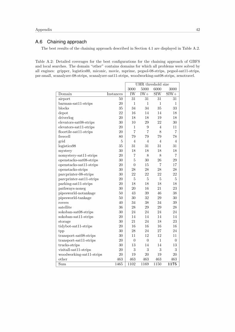
Appendix 42

A.6 Chaining approachThe best results of the chaining approach described in Section 4.1 are displayed in Table A.2.

Table A.2: Detailed coverages for the best configurations for the chaining approach of GBFSand local searches. The domain “other” contains domains for which all problems were solved byall engines: gripper, logistics00, miconic, movie, mprime, pegsol-08-strips, pegsol-sat11-strips,psr-small, scanalyzer-08-strips, scanalyzer-sat11-strips, woodworking-sat08-strips, zenotravel.

UHR threshold size3000 5000 6000 3000

Domain Instances IW IW+ SIW SIW+airport 50 31 31 31 31barman-sat11-strips 20 1 1 1 1blocks 35 34 34 35 33depot 22 16 14 14 18driverlog 20 18 18 19 18elevators-sat08-strips 30 10 29 22 30elevators-sat11-strips 20 1 9 4 11floortile-sat11-strips 20 7 7 8 7freecell 80 79 79 79 78grid 5 4 4 4 4logistics98 35 31 31 31 31mystery 30 18 18 18 18nomystery-sat11-strips 20 7 8 8 7openstacks-sat08-strips 30 5 30 26 29openstacks-sat11-strips 20 0 15 7 17openstacks-strips 30 28 28 28 28parcprinter-08-strips 30 22 22 22 22parcprinter-sat11-strips 20 5 5 5 5parking-sat11-strips 20 18 18 18 18pathways-noneg 30 20 16 21 23pipesworld-notankage 50 43 39 46 38pipesworld-tankage 50 30 32 29 30rovers 40 34 38 34 39satellite 36 28 29 29 28sokoban-sat08-strips 30 24 24 24 24sokoban-sat11-strips 20 14 14 14 14storage 30 21 24 18 23tidybot-sat11-strips 20 16 16 16 16tpp 30 28 24 27 24transport-sat08-strips 30 11 12 12 11transport-sat11-strips 20 0 0 1 0trucks-strips 30 13 14 14 13visitall-sat11-strips 20 3 3 3 3woodworking-sat11-strips 20 19 20 19 20other 463 463 463 463 463Sum 1465 1102 1169 1150 1175

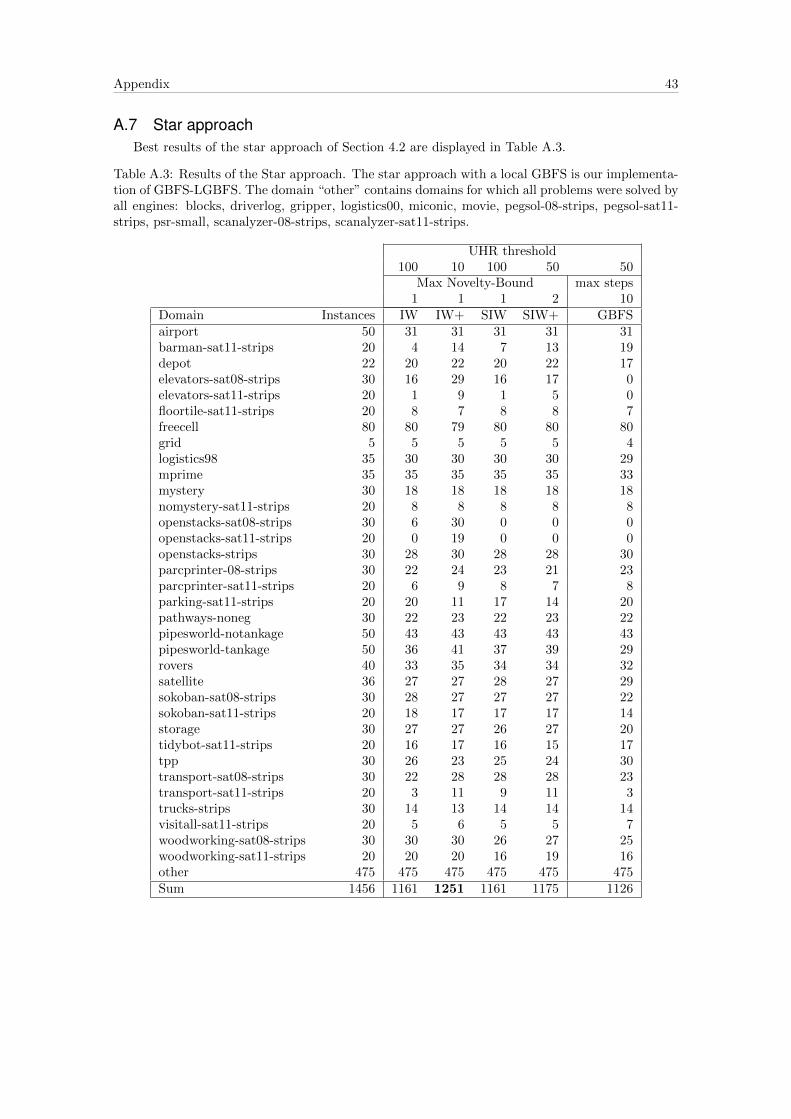
Appendix 43

A.7 Star approachBest results of the star approach of Section 4.2 are displayed in Table A.3.

Table A.3: Results of the Star approach. The star approach with a local GBFS is our implementa-tion of GBFS-LGBFS. The domain “other” contains domains for which all problems were solved byall engines: blocks, driverlog, gripper, logistics00, miconic, movie, pegsol-08-strips, pegsol-sat11-strips, psr-small, scanalyzer-08-strips, scanalyzer-sat11-strips.

UHR threshold100 10 100 50 50

Max Novelty-Bound max steps1 1 1 2 10

Domain Instances IW IW+ SIW SIW+ GBFSairport 50 31 31 31 31 31barman-sat11-strips 20 4 14 7 13 19depot 22 20 22 20 22 17elevators-sat08-strips 30 16 29 16 17 0elevators-sat11-strips 20 1 9 1 5 0floortile-sat11-strips 20 8 7 8 8 7freecell 80 80 79 80 80 80grid 5 5 5 5 5 4logistics98 35 30 30 30 30 29mprime 35 35 35 35 35 33mystery 30 18 18 18 18 18nomystery-sat11-strips 20 8 8 8 8 8openstacks-sat08-strips 30 6 30 0 0 0openstacks-sat11-strips 20 0 19 0 0 0openstacks-strips 30 28 30 28 28 30parcprinter-08-strips 30 22 24 23 21 23parcprinter-sat11-strips 20 6 9 8 7 8parking-sat11-strips 20 20 11 17 14 20pathways-noneg 30 22 23 22 23 22pipesworld-notankage 50 43 43 43 43 43pipesworld-tankage 50 36 41 37 39 29rovers 40 33 35 34 34 32satellite 36 27 27 28 27 29sokoban-sat08-strips 30 28 27 27 27 22sokoban-sat11-strips 20 18 17 17 17 14storage 30 27 27 26 27 20tidybot-sat11-strips 20 16 17 16 15 17tpp 30 26 23 25 24 30transport-sat08-strips 30 22 28 28 28 23transport-sat11-strips 20 3 11 9 11 3trucks-strips 30 14 13 14 14 14visitall-sat11-strips 20 5 6 5 5 7woodworking-sat08-strips 30 30 30 26 27 25woodworking-sat11-strips 20 20 20 16 19 16other 475 475 475 475 475 475Sum 1456 1161 1251 1161 1175 1126

Documents

Combining Novelty-Guided and Heuristic-Guided Searchai.cs.unibas.ch/papers/theses/maggi-master-16.pdf · Combining Novelty-Guided and Heuristic-Guided Search Master Thesis Natural