Embed Size (px)
Citation preview
Artificial Intelligence Review 21: 87–112, 2004.© 2004 Kluwer Academic Publishers. Printed in the Netherlands.
87
Combining Meta-Heuristics to Effectively Solve the VehicleRouting Problems with Time Windows
VINCENT TAM1 and K.T. MA2
1Department of Electrical and Electronic Engineering, The University of Hong Kong,Pokfulam Road, Hong Kong (E-mail: [email protected]);2Department of Computer Science, National University of Singapore, Lower Kent RidgeRoad, Singapore 119260 (Currently at Heuristix Lab Pte Ltd., Singapore;E-mail: [email protected])
Abstract. The vehicle routing problems with time windows are challenging delivery problemsin which instances involving 100 customers or more can be difficult to solve. There weremany interesting heuristics proposed to handle these problems effectively. In this paper, weexamined two well-known meta-heuristics and carefully combined the short-term and long-term memory-like mechanisms of both methods to achieve better results. Our prototype wasshown to compare favorably against the original search methods and other related searchhybrids on the Solomon’s test cases. More importantly, our proposal of integration opens upmany exciting directions for further investigation.
Keywords: guided local search, meta-heuristics, search hybrids, Tabu search, vehicle routingproblems
1. Introduction
Many delivery problems in real-world applications such as the newspaperdelivery and courier services can be formulated as capacitated vehicle routingproblems (VRPs) (Solomon 1987), which we want to route a number ofvehicles with limited capacity in order to satisfy customer requests with theminimal operational cost. This is usually measured by the number of vehiclesused multiplied by the total distance travelled. Often, a customer may specifya time-window with the earliest and latest time for the delivery, which givesrise to the VRP with time windows (VRP-TWs). In other words, a vehiclemust arrive at a customer within the interval as specified by that customer ina VRP-TWs. The arrival of a vehicle before the earliest time as specified by acustomer in a VRP-TWs will result in idle time. On the other hand, a vehicleis not allowed to reach a customer after the specified latest time. Moreover, aservice time is commonly associated with servicing each customer. A real-lifeexample of the VRP-TWs is furniture delivery in which each customer oftenrequests the furniture to be delivery within a given period of a day. Unfortu-
88 VINCENT TAM AND K.T. MA
nately, the VRP-TWs are shown to be NP-complete, implying an exponentialgrowth in the time complexity for a general algorithm to solve any of thesedelivery problems in the worst case. In practice, there are many instances ofVRP-TWs involving 100 customers (Backer et al. 1997; Solomon 1987) ormore (Seah 1999) which are difficult to solve optimally (Backer et al. 1997;Tsang et al. 1999; Jee 2000). In the past two decades, VRP-TWs, due totheir challenging nature and practical value, have continuously attracted manyinteresting proposals for useful heuristics and search algorithms (Backer et al.1997; Tsang et al. 1999) to effectively solve problems in the areas of ArtificialIntelligence (Tsang et al. 1999), Constraint Programming (Backer et al. 1997)and Operations Research (Tsang et al. 1999).
Among the heuristics (Backer et al. 1997; Kilby et al. 1997) proposed tosolve the vehicle routing problems, there are some interesting proposals toinitialize the search while others are targeted at advancing the search froma given initial state in an effective manner. As far as search initialization isconcerned, there are two useful heuristics, namely the push-forward insertionheuristic (PFIH) (Jee 2000) and the virtual vehicle heuristic (VVH) (Kilbyet al. 1997) which was proposed to generate more feasible initial statesthat may lead to better results. The PFIH is a simple-yet-efficient methodto compute every route by comparing the cost of inserting a new customerinto the existing route against that of starting a new route in each iterationuntil all customers are served. However, when the capacity of a vehicle isexceeded or the delivery time must be dragged behind the latest time specifiedby the new customer, a new route has to be started. Clearly, the PFIH canonly quickly return a feasible solution without any guarantee for its globaloptimality. On the other hand, the VVH works by using virtual vehicles withunlimited capacity to hold the deliveries that are not currently serviced by anyreal vehicle so as to allow a more optimized delivery plan to be computed. Inother words, the virtual vehicles are used as temporary buffers to which noproblem constraints (such as time and capacity) can be applied. Furthermore,to ensure all the deliveries will ultimately be performed by real vehicles, thecost incurred by a virtual vehicle for a customer visit is much higher thanthat incurred by a real vehicle. In this paper, we will focus on comparingthe influence of the above initialization heuristics on search meta-heuristics.Section 3 will present a more detailed discussion on the initializationheuristics.
After the initial routes for the VRPs are generated, we can apply manypossible heuristic methods to improve on the current solution until a betterdelivery plan with lower operational cost is obtained. The Tabu search (TS)(Backer et al. 1997) is a well-known meta-heuristic possibly used for suchimprovement, which has also been successfully applied to solve many other
VEHICLE ROUTING PROBLEMS 89
combinatorial optimization problems (Tsang et al. 1999). In solving VRPs,given any initial route(s), there can be many possible moves (Backer et al.1997) such as the 2-opt operation, which replaces any two links in a route withtwo different links to reduce the operational cost, to generate other possibleroute(s). The Tabu search works by firstly performing a neighborhood searchon all possible moves, executing only non-Tabu moves which reduce the totaloperational cost, and ‘memorizing’ those recently performed moves with aTabu list, usually of fixed length, to avoid cycling. In this way, TS promotesa diversified search from the current solution by continuously updating ashort-term memory-like Tabu list until the predetermined stopping criterionis reached. In some cases, depending on the application-specific aspirationlevel criterion, the Tabu status of a move can be changed when it leads to asolution better than the current best. Alternatively, the guided local search(GLS) (Kilby et al. 1997; Tsang et al. 1999) is another interesting meta-heuristic which has also achieved impressive results (Kilby et al. 1997) insolving VRP-TWs effectively. Both TS and GLS are based on a local searchoperator to perform neighborhood search. However, each time after the localsearch is performed, the GLS uses a long-term memory-like penalty schemeto penalize all the undesirable features found in the current solution so asto avoid being trapped at the same local minima in future exploration. Theresulting penalty information, after multiplied by a regularization parameterλ, is incorporated into an augmented objective function to guide the localsearch to iteratively look for a better solution from the current search positionuntil a predefined stopping condition such as the maximum number of itera-tions is reached. In addition to solving VRPs, GLS has been successfullyapplied to solve many difficult scheduling problems such as the travelingsalesman problem (Voudouris and Tsang 1995).
Previous work (Backer et al. 1997; Kilby et al. 1997) proposed to combinethe possible advantages of different meta-heuristics for solving constrainedoptimization problems or in particular VRPs more efficiently or effectively.Wah et al. (2000) considered the integration of simulated annealing tech-nique in a Discrete Lagrangian search framework, which was closely relatedto GLS, as constrained simulated annealing (CSA) to solve a set of 10constrained optimization problems (named G1–G10) (Wah and Chen 2000)with constraints and objective functions of various types. Later, the CSAwas further improved with a genetic algorithm as CSAGA to achieve abetter efficiencyin solving the same set of constrained optimization problems.Specifically, Genfreau et al. (1994) integrated simulated annealing and Tabusearch to effectively solve VRPs. Interestingly, Becker et al. (1997), aftercomparing the individual performance of GLS and TS on the Solomon’s testcases, tried to combine both TS and GLS as the guided Tabu search (GTS)
90 VINCENT TAM AND K.T. MA
method which outperformed the original meta-heuristics with an average of1.7% better1 in the solution quality on the “long haul” problems, that areproblems involving deliveries of long distances. However, Becker et al.’swork suffered from three major drawbacks. First, their original aim, possiblyonly to obtain better experimental results, for combining both meta-heuristicswas never explicitly stated. Second, the algorithm of the GTS was not clearlydefined. There were only 3 statements to describe GTS very briefly. Third,no analytical model or clear explanation about the performance of GTS wasgiven. On the other hand, we carefully propose in this paper a differentintegration of GLS and TS as GLS-TS with a clear objective to combinethe best possible advantages of applying both the short-term and long-termmemory mechanism used in GLS and TS to solve VRP-TWs more effectively.More importantly, we provide a simple and easy-to-understand analyticalmodel to understand the behavior of the resulting GLS-TS when comparedto the original meta-heuristics. Furthermore, similar to Wah et al.’s work(2000), we propose the integration of simulated annealing technique intothe GLS-TS search framework as GLS-TS-SA. However, it is worth notingthat simulated annealing is specially used as a monitor in GLS-TS-SA tocarefully determine, depending on the relative merit of each meta-heuristicin the previous search, which meta-heuristic to apply in each iteration. Todemonstrate the effectiveness of our proposals in solving VRP-TWs, weimplemented the prototypes of both GLS-TS and its variant GLS-TS-SA.Both prototypes have been shown to compare very favorably in the solutionquality against the original GLS and TS methods, and the search hybrid GTSon the well-known Solomon’s test cases (Solomon 1987) which have beenused as standard benchmarks for comparing the performance of differentsearch strategies for decades. In addition, our proposed GLS-TS improvedon one of the best published results, which were obtained from a number ofadvanced search techniques such as the Ant Colony search algorithm (Seah1999) and thus fairly difficult to break any of these records, in solving theSolomon’s benchmarks on VRP-TWs. To our knowledge, this work repre-sents the first attempt to systematically study the integration of TS into theGLS search framework.
This paper is organized as follows. Section 2 describes the general vehiclerouting problems and VRP-TWs in detail. The various search initializationheuristics such as the PFIH, interesting meta-heuristics such as the TabuSearch and combined meta-heuristics such as the Guided Tabu Search (GTS)to effectively solve VRP-TWs will be given in Section 3. Section 4 detailsour proposals of adapting the generic MGA to solve the VRP-TWs moreeffectively. In Section 5, we evaluate the performance of our proposal against
VEHICLE ROUTING PROBLEMS 91
the original heuristic search methods and the related GTS on the widely usedSolomon test cases. Lastly, we conclude our work in Section 5.
2. The Vehicle Routing Problems with Time Windows
A general vehicle routing problem (VRP) (Backer et al. 1997; Solomon1987), which is shown to be NP-complete (Tsang et al. 1999), can beformally defined as follows. We are given a fixed N or infinite number ofvehicles with limited capacity cv (measured in weight or volume) and Mcustomers’ requests, in which each request rqj demands a delivery servicefor Qj quantity of goods/service, to different locations. The distance, usuallymeasured in term of minutes or hours required for travel, between any twopossible delivery points is also provided, usually as a distance matrix. Then,our task is to optimize certain user-defined criteria subject to the followingbasic constraints:1. any customer request rqj should only be served by one vehicle only;2. for each vehicle v, the sum Qv of quantity of goods to be delivered by
vehicle v must be less than or equal to cv.Besides the above basic constraints, in many real-life applications such as
supermarket delivery, each customer may request the items to be deliveredin a given period (time window) of a day. Thus, a vehicle routing problemwith time windows (VRP-TW) has an additional time-window constraint tobe imposed for each delivery as follows.3. when a time window with the earliest time Ej and the latest time Lj is
specified for each delivery in a VRP-TW, the arrival time Tvj of vehicle vto serve customer request rqj must lie within the specified duration, thatis Ej ≤ Tvj ≤ Lj .
One of the most common objectives for minimization in VRPs or VRP-TWs is TV × TD, where TV is the number of vehicles used, and TD is the totaldistance travelled by all vehicles. Throughout this paper, our compared searchstrategies work to minimize this common objective of TV × TD. Clearly,there can be many variants of VRPs or VRP-TWs with different objectivessuch as the total travel time of all the vehicles or the total waiting time ofall the customers for optimization in many real-life applications. In the nextsection, we examine two common heuristics, namely the push-forward inser-tion heuristic and the virtual vehicle heuristic, useful to obtain an initial andfeasible solution in solving the VRPs or VRP-TWs. Moreover, we will reviewtwo interesting meta-heuristics to solve the difficult VRP-TWs optimally.
92 VINCENT TAM AND K.T. MA
3. Useful Heuristics and Meta-Heuristics for Vehicle Routing
Since the search space for all the possible (feasible or slightly infeasible)routes in VRPs or VRP-TWs can be fairly large even for instances involving100 customers (Backer et al. 1997; Solomon 1987) or more (Seah 1999),and the time-window constraints in the VRP-TWs can be difficult to satisfy,the careful choice of a suitable heuristic to return only feasible, and possiblymore optimal, solutions can be important for further optimization. The push-forward insertion heuristic (Jee 2000) and virtual vehicle heuristic (Kilby etal. 1997) are two useful heuristics for search initialization in solving difficultVRPs. In addition, we will examine in this section two well-known meta-heuristics, namely the guided local search (GLS) and Tabu search (TS),which are based on completely different memory-like control mechanismsto restrict the local search operator in continuously optimizing the currentsolution, after input from the heuristic initialization method, until an optimalsolution is obtained to solve the VRP-TWs successfully. TS uses a short-termmemory-like Tabu list to avoid cycles in search. On the other hand, GLS usesa long-term memory-like penalty scheme to “memorize” all the undesirablefeatures occurring in the previously visited local minima. In Section 4, wewill examine various proposals to integrate TS into the GLS framework tosolve VRP-TWs more effectively.
3.1. Useful search initialization heuristics
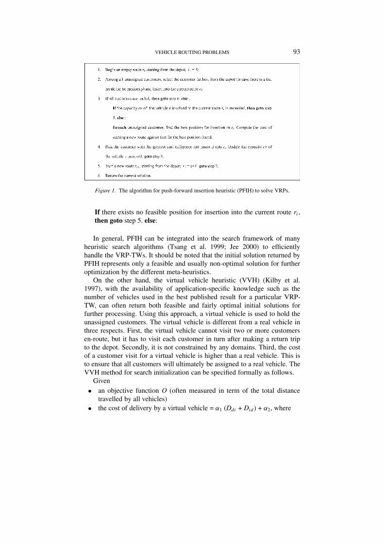
The push-forward insertion heuristic (PFIH) (Solomon 1987), introduced bySolomon in 1987, is an efficient method to compute a feasible solution forany VRP by assuming an infinite number of vehicles. The PFIH starts a newroute by selecting an initial customer, usually farthest from the delivery depot,and then iteratively inserts any unassigned customer into the current routeuntil the capacity of the current vehicle is exceeded or the waiting time forany newly added customer will exceed its associated duration constraint. Atthis moment, a new route will be created. And this process repeats until allcustomers are served. Basically, the algorithm for PFIH can be summarizedin Figure 1.
Clearly when handling VRP-TWs, we have to adapt the last else-part ofstep 3 as follows.
for each unassigned customer, find the best position for insertion inri without violating any specified time-window. Compute the cost ofstarting a new route against that for the best position found.
Moreover, we have to add the following conditional statement to thebeginning of step 4 as follows.
VEHICLE ROUTING PROBLEMS 93
Figure 1. The algorithm for push-forward insertion heuristic (PFIH) to solve VRPs.
If there exists no feasible position for insertion into the current route ri ,then goto step 5. else:
In general, PFIH can be integrated into the search framework of manyheuristic search algorithms (Tsang et al. 1999; Jee 2000) to efficientlyhandle the VRP-TWs. It should be noted that the initial solution returned byPFIH represents only a feasible and usually non-optimal solution for furtheroptimization by the different meta-heuristics.
On the other hand, the virtual vehicle heuristic (VVH) (Kilby et al.1997), with the availability of application-specific knowledge such as thenumber of vehicles used in the best published result for a particular VRP-TW, can often return both feasible and fairly optimal initial solutions forfurther processing. Using this approach, a virtual vehicle is used to hold theunassigned customers. The virtual vehicle is different from a real vehicle inthree respects. First, the virtual vehicle cannot visit two or more customersen-route, but it has to visit each customer in turn after making a return tripto the depot. Secondly, it is not constrained by any domains. Third, the costof a customer visit for a virtual vehicle is higher than a real vehicle. This isto ensure that all customers will ultimately be assigned to a real vehicle. TheVVH method for search initialization can be specified formally as follows.
Given• an objective function O (often measured in term of the total distance
travelled by all vehicles)• the cost of delivery by a virtual vehicle = α1 (Ddi + Did) + α2, where
94 VINCENT TAM AND K.T. MA
– Dij is the distance between customers ci and cj with d as the depot,– α1 and α2 are parameters set to increase the cost of a visit by the
virtual vehicle,the VVH algorithm proceeds as follow.1. The virtual vehicle services all the customers’ requests.2. For each customer-vehicle combination in the current solution, use 4
heuristic operators, namely the 2-opt, relocate, exchange and cross, to tryto improve the solution quality by firstly considering only legal movesthat do not violate any constraint, and then executing the legal movewhich decreases the objective function most.
3. If no more customer-vehicle combination can be improved to reduce thesolution quality, goto step 5.
4. goto step 2.5. return the current solution.
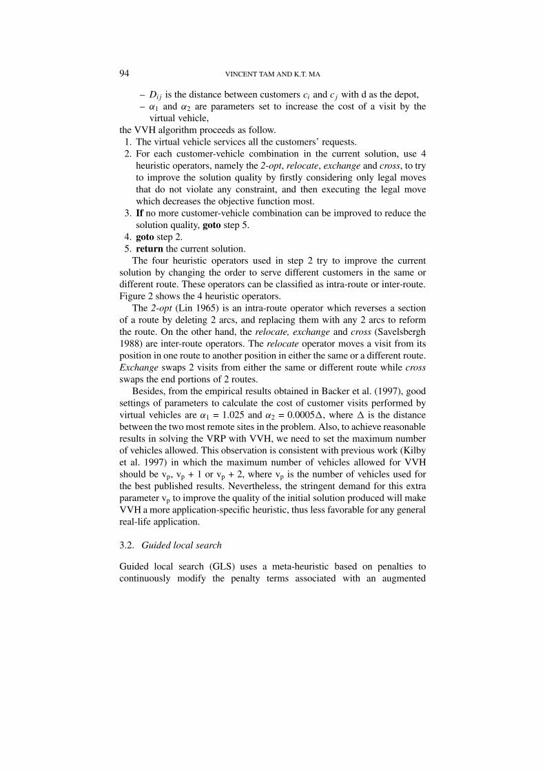
The four heuristic operators used in step 2 try to improve the currentsolution by changing the order to serve different customers in the same ordifferent route. These operators can be classified as intra-route or inter-route.Figure 2 shows the 4 heuristic operators.
The 2-opt (Lin 1965) is an intra-route operator which reverses a sectionof a route by deleting 2 arcs, and replacing them with any 2 arcs to reformthe route. On the other hand, the relocate, exchange and cross (Savelsbergh1988) are inter-route operators. The relocate operator moves a visit from itsposition in one route to another position in either the same or a different route.Exchange swaps 2 visits from either the same or different route while crossswaps the end portions of 2 routes.
Besides, from the empirical results obtained in Backer et al. (1997), goodsettings of parameters to calculate the cost of customer visits performed byvirtual vehicles are α1 = 1.025 and α2 = 0.0005�, where � is the distancebetween the two most remote sites in the problem. Also, to achieve reasonableresults in solving the VRP with VVH, we need to set the maximum numberof vehicles allowed. This observation is consistent with previous work (Kilbyet al. 1997) in which the maximum number of vehicles allowed for VVHshould be vp, vp + 1 or vp + 2, where vp is the number of vehicles used forthe best published results. Nevertheless, the stringent demand for this extraparameter vp to improve the quality of the initial solution produced will makeVVH a more application-specific heuristic, thus less favorable for any generalreal-life application.
3.2. Guided local search
Guided local search (GLS) uses a meta-heuristic based on penalties tocontinuously modify the penalty terms associated with an augmented
VEHICLE ROUTING PROBLEMS 95
Figure 2. The 4 heuristic operators for improving routes in solving VRPs.
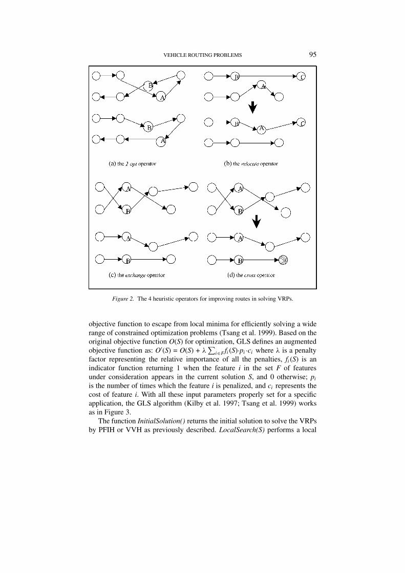
objective function to escape from local minima for efficiently solving a widerange of constrained optimization problems (Tsang et al. 1999). Based on theoriginal objective function O(S) for optimization, GLS defines an augmentedobjective function as: O′(S) = O(S) + λ
∑i∈F fi(S)·pi ·ci where λ is a penalty
factor representing the relative importance of all the penalties, fi(S) is anindicator function returning 1 when the feature i in the set F of featuresunder consideration appears in the current solution S, and 0 otherwise; pi
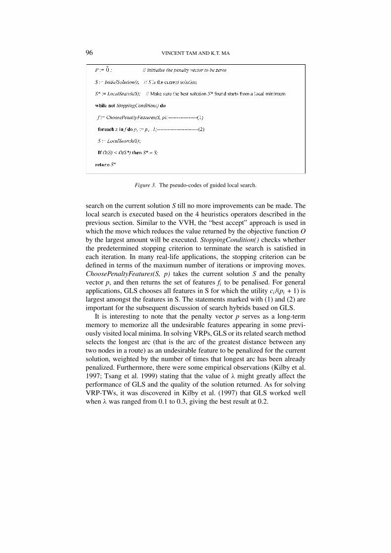
is the number of times which the feature i is penalized, and ci represents thecost of feature i. With all these input parameters properly set for a specificapplication, the GLS algorithm (Kilby et al. 1997; Tsang et al. 1999) worksas in Figure 3.
The function InitialSolution() returns the initial solution to solve the VRPsby PFIH or VVH as previously described. LocalSearch(S) performs a local
96 VINCENT TAM AND K.T. MA
Figure 3. The pseudo-codes of guided local search.
search on the current solution S till no more improvements can be made. Thelocal search is executed based on the 4 heuristics operators described in theprevious section. Similar to the VVH, the “best accept” approach is used inwhich the move which reduces the value returned by the objective function Oby the largest amount will be executed. StoppingCondition() checks whetherthe predetermined stopping criterion to terminate the search is satisfied ineach iteration. In many real-life applications, the stopping criterion can bedefined in terms of the maximum number of iterations or improving moves.ChoosePenaltyFeatures(S, p) takes the current solution S and the penaltyvector p, and then returns the set of features fi to be penalised. For generalapplications, GLS chooses all features in S for which the utility ci /(pi + 1) islargest amongst the features in S. The statements marked with (1) and (2) areimportant for the subsequent discussion of search hybrids based on GLS.
It is interesting to note that the penalty vector p serves as a long-termmemory to memorize all the undesirable features appearing in some previ-ously visited local minima. In solving VRPs, GLS or its related search methodselects the longest arc (that is the arc of the greatest distance between anytwo nodes in a route) as an undesirable feature to be penalized for the currentsolution, weighted by the number of times that longest arc has been alreadypenalized. Furthermore, there were some empirical observations (Kilby et al.1997; Tsang et al. 1999) stating that the value of λ might greatly affect theperformance of GLS and the quality of the solution returned. As for solvingVRP-TWs, it was discovered in Kilby et al. (1997) that GLS worked wellwhen λ was ranged from 0.1 to 0.3, giving the best result at 0.2.

VEHICLE ROUTING PROBLEMS 97
Figure 4. The pseudo-codes of Tabu search.
3.3. Tabu search
Tabu search is an interesting meta-heuristic which aims to model the humanmemory process through the use of a Tabu list, usually of a fixed length, toprohibit most recent moves possibly leading to some previously visited localoptima. In solving VRP-TWs (Backer et al. 1997; Solomon 1987), movescan be defined in term of the addition or deletion of arcs associated withindividual nodes (as customers) into or out of all computed routes. Besidesthe Tabu list, an aspiration criterion is used to change the Tabu status of amove so that the move in the Tabu list can still be accepted when it leads to asolution better than the current best solution. In general, the performance ofa Tabu search algorithm depends largely on effectiveness of the local searchoperators, the length of the Tabu list and the settings used for the aspirationcriterion. Nevertheless, Tabu search has been extensively used to solve manydifficult combinatorial problems with good results (Backer et al. 1997).
Figure 4 gives the Tabu search algorithm as described in (Backer et al.1997; Kilby et al. 1997).
The search starts with an initial solution S provided by InitialSolution().Then, LocalSearch(S) uses the four heuristic intra-route and inter-route opera-
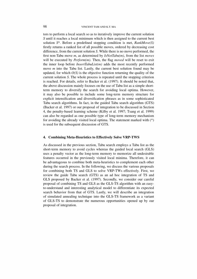
98 VINCENT TAM AND K.T. MA
tors to perform a local search so as to iteratively improve the current solutionS until it reaches a local minimum which is then assigned to the current bestsolution S*. Before a predefined stopping condition is met, RankMove(S)firstly returns a ranked list of all possible moves, ordered by decreasing costdifference, from the current solution S. While there is no move performed, thefirst non-Tabu move m, as determined by IsNotTabu(m), from the list moveswill be executed by Perform(m). Then, the flag moved will be reset to exitthe inner loop before InsertTabuList(m) adds the most recently performedmove m into the Tabu list. Lastly, the current best solution found may beupdated, for which O(S) is the objective function returning the quality of thecurrent solution S. The whole process is repeated until the stopping criterionis reached. For details, refer to Backer et al. (1997). It should be noted that,the above discussion mainly focuses on the use of Tabu list as a simple short-term memory to diversify the search for avoiding local optima. However,it may also be possible to include some long-term memory structure forexplicit intensification and diversification phrases as in some sophisticatedTabu search algorithms. In fact, in the guided Tabu search algorithm (GTS)(Backer et al. 1997) or our proposal of integration to be discussed in Section4, the penalty-based learning scheme (Kilby et al. 1997; Tsang et al. 1999)can also be regarded as one possible type of long-term memory mechanismfor avoiding the already visited local optima. The statement marked with (*)is used for the subsequent discussion of GTS.
4. Combining Meta-Heuristics to Effectively Solve VRP-TWS
As discussed in the previous section, Tabu search employs a Tabu list as theshort-term memory to avoid cycles whereas the guided local search (GLS)uses a penalty vector as the long-term memory to memorize all undesirablefeatures occurred in the previously visited local minima. Therefore, it canbe advantageous to combine both meta-heuristics to complement each otherduring the search process. In the following, we discuss the various proposalsfor combining both TS and GLS to solve VRP-TWs effectively. First, wereview the guide Tabu search (GTS) as an ad hoc integration of TS andGLS proposed by Backer et al. (1997). Secondly, we consider our carefulproposal of combining TS and GLS as the GLS-TS algorithm with an easy-to-understand and interesting analytical model to differentiate its expectedsearch behavior from that of GTS. Lastly, we will describe an integrationof simulated annealing technique into the GLS-TS framework as a variantof GLS-TS to demonstrate the numerous opportunities opened up by ourproposal of integration.
VEHICLE ROUTING PROBLEMS 99
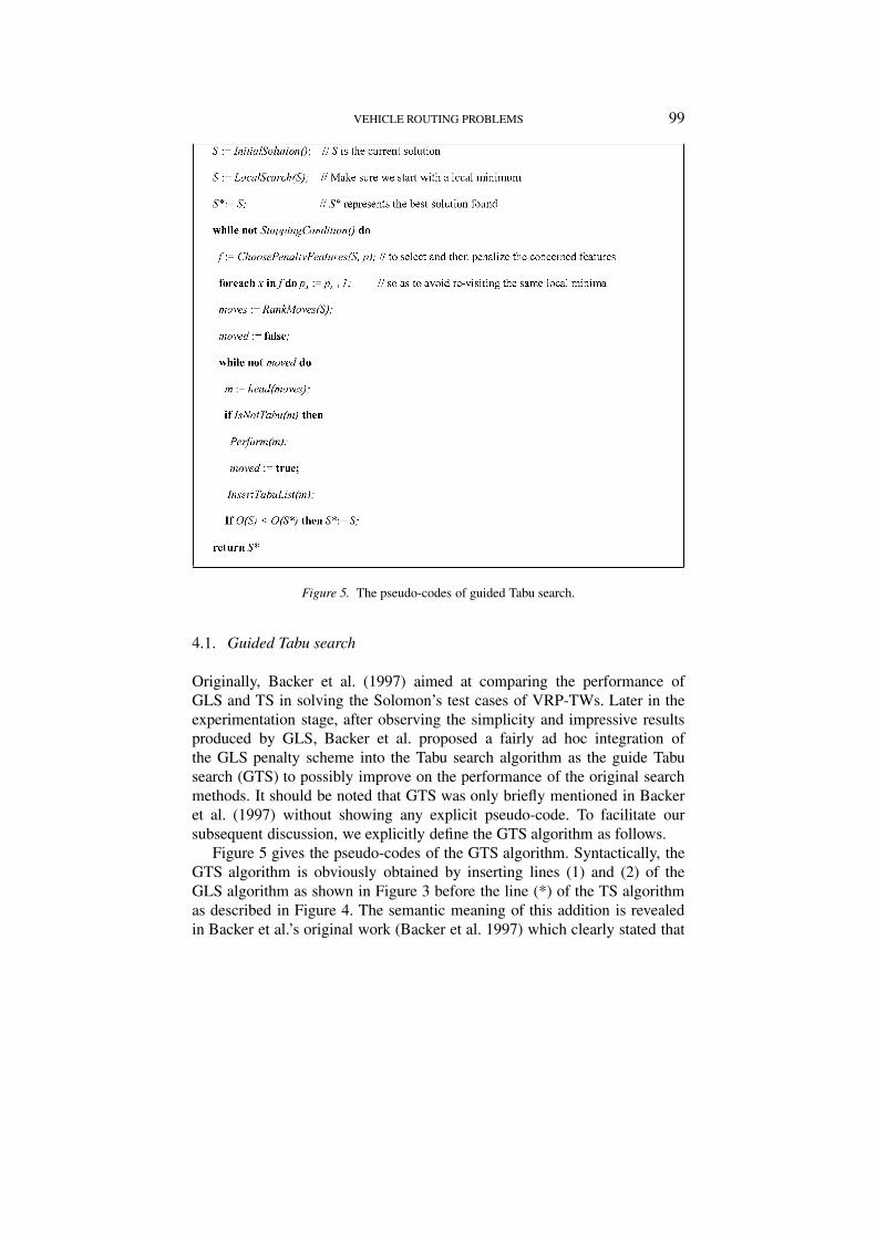
Figure 5. The pseudo-codes of guided Tabu search.
4.1. Guided Tabu search
Originally, Backer et al. (1997) aimed at comparing the performance ofGLS and TS in solving the Solomon’s test cases of VRP-TWs. Later in theexperimentation stage, after observing the simplicity and impressive resultsproduced by GLS, Backer et al. proposed a fairly ad hoc integration ofthe GLS penalty scheme into the Tabu search algorithm as the guide Tabusearch (GTS) to possibly improve on the performance of the original searchmethods. It should be noted that GTS was only briefly mentioned in Backeret al. (1997) without showing any explicit pseudo-code. To facilitate oursubsequent discussion, we explicitly define the GTS algorithm as follows.
Figure 5 gives the pseudo-codes of the GTS algorithm. Syntactically, theGTS algorithm is obviously obtained by inserting lines (1) and (2) of theGLS algorithm as shown in Figure 3 before the line (*) of the TS algorithmas described in Figure 4. The semantic meaning of this addition is revealedin Backer et al.’s original work (Backer et al. 1997) which clearly stated that
100 VINCENT TAM AND K.T. MA
after each move, a GLS-type procedure was called to update the weight in thecost matrix (used in the penalty scheme). However, we consider this frequentinvocation of the GLS-type procedure may collect “immature and hazardous”penalty information after every single diversifying move of TS. The collectedpenalty information can be “hazardous” in two senses. First, it can mislead thecurrent search direction by biasing towards some unimportant features foundin the previous solutions. Second, the vast amount of possibly useless penaltyinformation generated may simply cause information or memory overflowduring program execution. Besides, it may slow down the performance ofGTS. In the next subsection, we will provide an interesting and simple modelto carefully consider the possible influence of this frequent penalty mech-anism on the search behavior of GTS. After all, from Backer et al.’s empiricalexperience (Backer et al. 1997), GTS showed some benefits by outperformingthe TS and GLS with an average of 1.7% on long-haul problems, includingC2, R2 and RC2, of the Solomon’s test cases. However, for the remainingproblem classes, GTS did not show any convincing result when compared toGLS.
4.2. Our proposed guided local search – Tabu search (GLS-TS)
As previously discussed, the guided Tabu search (GTS) did not seem to be anattractive proposal for integrating GLS and TS since the short-term memorynature of the TS may not be able to effectively use the long-term memory-like penalty information frequently provided by the GLS scheme to diversifythe search from its current status. In other words, the GLS scheme maypenalize some features which will be totally irrelevant to the current state ofTS. Therefore, we propose an alternative integration: instead of performing asingle non-Tabu move for every update of the cost matrix used in the penaltyscheme, we propose to update the penalties only when the TS reaches a stablestate. In other words, the penalties are updated only when all the non-Tabumoves cannot further improve the current solution any more.
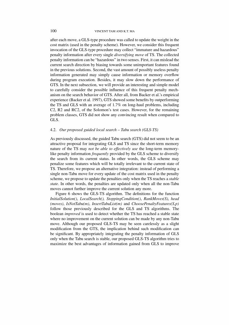
Figure 6 shows the GLS-TS algorithm. The definitions for the functionInitialSolution(), LocalSearch(), StoppingCondition(), RankMoves(S), head(moves), IsNotTabu(m), InsertTabuList(m) and ChoosePenaltyFeatures(S,p)follow those previously described for the GLS and TS algorithms. Theboolean improved is used to detect whether the TS has reached a stable statewhere no improvement on the current solution can be made by any non-Tabumove. Although our proposed GLS-TS may be seen carelessly as a slightmodification from the GTS, the implication behind such modification canbe significant. By appropriately integrating the penalty information of GLSonly when the Tabu search is stable, our proposed GLS-TS algorithm tries tomaximize the best advantages of information gained from GLS to improve
VEHICLE ROUTING PROBLEMS 101
Figure 6. The pseudo-codes of guided local search – Tabu search (GLS-TS).
the original Tabu search. This competitive advantage of GLS-TS whencompared to GTS is illustrated clearly in the following simplified Markovchain diagrams to analyse their different search behaviour in successfullyfinding a solution for general and solvable VRPs.
Figure 7 gives the simplified Markov models for the original TS, GTSand GLS-TS algorithms which successfully find a solution for a general andsolvable VRP. Each circle in the diagram is a (search) state representing the
102 VINCENT TAM AND K.T. MA
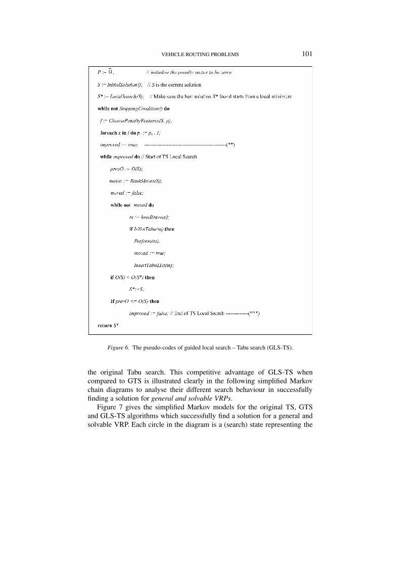
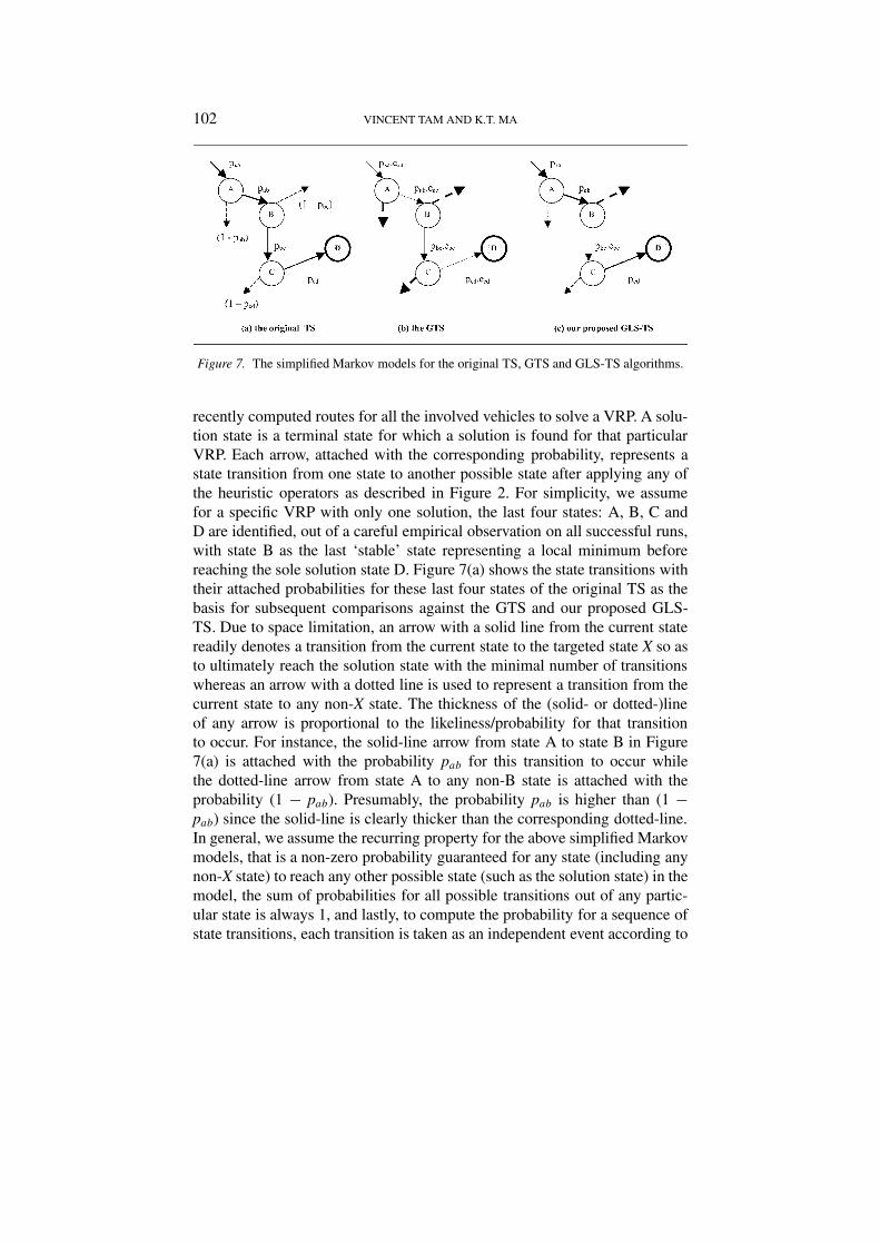
Figure 7. The simplified Markov models for the original TS, GTS and GLS-TS algorithms.
recently computed routes for all the involved vehicles to solve a VRP. A solu-tion state is a terminal state for which a solution is found for that particularVRP. Each arrow, attached with the corresponding probability, represents astate transition from one state to another possible state after applying any ofthe heuristic operators as described in Figure 2. For simplicity, we assumefor a specific VRP with only one solution, the last four states: A, B, C andD are identified, out of a careful empirical observation on all successful runs,with state B as the last ‘stable’ state representing a local minimum beforereaching the sole solution state D. Figure 7(a) shows the state transitions withtheir attached probabilities for these last four states of the original TS as thebasis for subsequent comparisons against the GTS and our proposed GLS-TS. Due to space limitation, an arrow with a solid line from the current statereadily denotes a transition from the current state to the targeted state X so asto ultimately reach the solution state with the minimal number of transitionswhereas an arrow with a dotted line is used to represent a transition from thecurrent state to any non-X state. The thickness of the (solid- or dotted-)lineof any arrow is proportional to the likeliness/probability for that transitionto occur. For instance, the solid-line arrow from state A to state B in Figure7(a) is attached with the probability pab for this transition to occur whilethe dotted-line arrow from state A to any non-B state is attached with theprobability (1 − pab). Presumably, the probability pab is higher than (1 −pab) since the solid-line is clearly thicker than the corresponding dotted-line.In general, we assume the recurring property for the above simplified Markovmodels, that is a non-zero probability guaranteed for any state (including anynon-X state) to reach any other possible state (such as the solution state) in themodel, the sum of probabilities for all possible transitions out of any partic-ular state is always 1, and lastly, to compute the probability for a sequence ofstate transitions, each transition is taken as an independent event according to
VEHICLE ROUTING PROBLEMS 103
the theory of Probability (Hoel 1976). Therefore, given the recurring propertyof the simplified Markov model, the probability of reaching the solution stateD from any non-X state is always 1/(N − 1) where N is the total number ofpossible states in the simplified model. Hence, the probability of reachingfrom state A successfully to state D equals to pab·pbc·pcd + (1 − pab). 1/(N− 1) + pab·(1 − pbc). 1/(N − 1), in which and the second term (1 − pab).1/(N − 1) gives the probability of reaching from state A to non-B state andfinally to state D. Furthermore, we assume the probability of reaching fromany previous state to state A is greater than 0.5 so that the probability ofsuccessfully reaching state D largely depends on the decisions made in thelast four states. Since the three probabilities pab, pbc and pcd normally rangefrom 0 to 1, and N is at least of the order of 1,000 or more, the first termpab·pbc·pcd is usually the most important quantity to consider in determiningthe probability of reaching from state A to state D. To illustrate, let pab, pbc
and pcd be 0.4, 0.5 and 0.6 respectively, and N be 1,000, the probability ofreaching from state A to state D equals to 0.4 × 0.5 × 0.6 + (1 − 0.4)× 1/999 + 0.4 × (1 − 0.5) × 1/999 = 0.12 + 0.0006 + 0.0002 = 0.1208in which the first term is clearly the most determining factor. However inthe GTS, by including the GLS penalty mechanism in every step of the TS,we assume the probability of a transition (A → B) being affected by theGLS penalties as gab, and conversely the probability of not being affectedas eab = 1 − gab. Similarly, all of these e’s and g’s will be in the range of0 to 1. Moreover, the g’s should be progressively increasing from the initialto the last state since there can be more features to be penalized or higherpenalty resulted after each iteration which may affect the state transition ofthe original TS more drastically. Overall, applying the GLS penalty schemein each TS step will substantially lower the first important term of the proba-bility of successfully reaching from state A to state D, at least by the order of10−3, to pab·pbc·pcd ·eab·ebc·ecd which cannot be offset by the relatively smallopposite increase in the second and third terms of the specific probability dueto the very small increase in the probability of reaching the non-B and non-C states from state A and B. This clearly shows the possible pitfalls of theGTS proposal which may simply increase the chance of diverting the currentsearch to some unintentional states, that are any states other than the solutionstate D in the non-B and non-C states. On the other hand, by intelligentlymaintaining the original characteristics of the TS and only affect the TS by theGLS penalty mechanism in stable states like state B in our proposed GLS-TSas shown Figure 7(c), the original strength as reflected in the first importantterm of the probability of reaching from state A to D is largely unaffectedby multiplying only one ebc as pab·pbc·ebc· pcd . Meanwhile, the probabilityof reaching non-C states at the stable state B is appropriately increased to
104 VINCENT TAM AND K.T. MA
open up a risky but possibly favorite opportunity to try to directly reach thesolution state D. Also, it is worthy noting that since the system already arrivesat the stable state B, there is a fair chance of re-entering the same stable stateB even after it fails to reach the solution state D. In other words, we carefullyinject some intended noise into the original search model of TS (as shown inFigure 7(a)) to increase the chance of directly reaching the solution state(s)only at stable states while not drastically scarifying the original strength, thatis a higher probability of following the normal transitions from A → B →C → D, of TS in our proposed GLS-TS. After all, Section 5 will give theexperimental results of the original TS, the GTS and our proposed GLS-TS on the well-known Solomon’s benchmarks (Solomon 1987) to justify ourdiscussion here.
4.3. Yet another variant of GLS-TS
Both GTS and our proposed GLS-TS are basically fixed strategies to invokethe GLS-type penalty scheme within the TS framework, it will be interestingto have other variants of GLS-TS which can flexibly invoke different searchmechanisms depending on the relative merit of the involved mechanismsduring the dynamic search process. Basically, we need a kind of measure anda monitor as the feedback-and-control mechanism of this flexible invocationscheme. Similar to Wah et al.’s work (Wah and Chen 2000), we proposeto integrate simulated annealing as a monitor to supervise the performanceof different search mechanisms and decide which mechanism to invoke ineach stage of the search. This forms the basis of our proposed GLS-TS-SAalgorithm as a variant of GLS-TS. This will decide whether to invoke thecommon local search method used in GLS or the unique Tabu search methodduring the search process. For testing, we simply used the number of accumu-lated improving moves made by each search method as a score to measuretheir relative merit. Obviously, there can be more sophisticated measuresdefined to evaluate their performance. More importantly, our proposal ofintegration discussed here opens up many potentially interesting directionsfor future investigation.
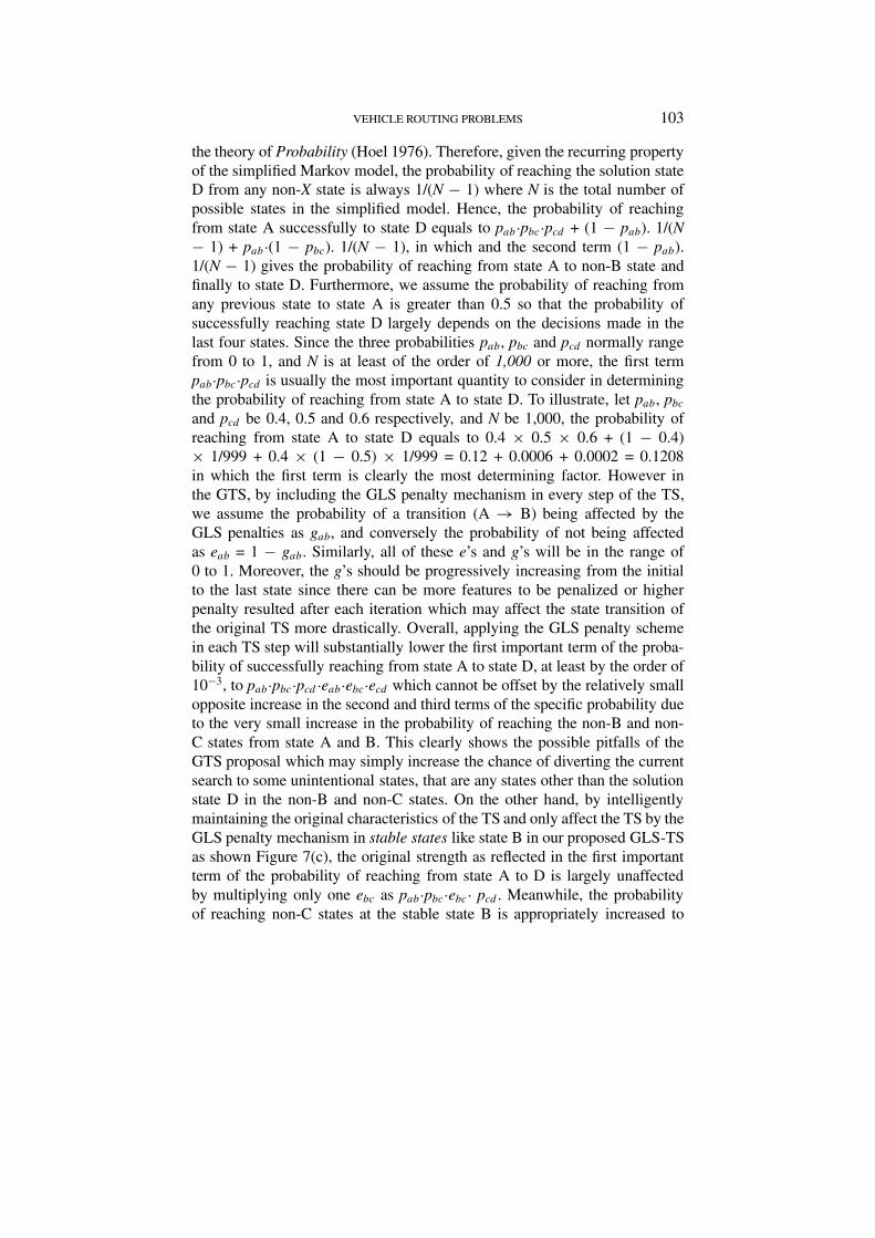
Figure 8 gives the pseudo-codes of the GLS-TA integrated with simu-lated annealing. InitialSolution(), LocalSearch(), StoppingCondition() andChoosePenaltyFeatures(S,p) are as described in the GLS-TS algorithm inFigure 6. Random(0,1) generates a random real number between 0 and 1.The function Tabu-LocalSearch() basically performs a Tabu search until nomore improvements for the objective function is achieved. The variable icounts number of times the variant GLS-TS-SA performs a Tabu search whilethe counter impM measures the number of accumulative improving movesaffected by Tabu search. The variable d represents the decrease in the total
VEHICLE ROUTING PROBLEMS 105
Figure 8. The pseudo-codes for the GLS – Tabu search integrated with simulated annealing(GLS-TS-SA).
distance traveled, which is either 0 or −d for any increase. The parameterMAX_TEMP was empirically determined at 0.3. In addition, the formulationfor temp and Pcalc basically follows the standard logistic function described in(Spears 1993). Besides our proposed GLS-TS-SA, we can clearly have manyother possible search hybrids integrated with simulated annealing such as anadaptive strategy which can flexibly invoke the GLS penalty scheme withinthe TS framework depending on its performance. Some of these proposalsform our on-going work.
106 VINCENT TAM AND K.T. MA
5. Experimental Results
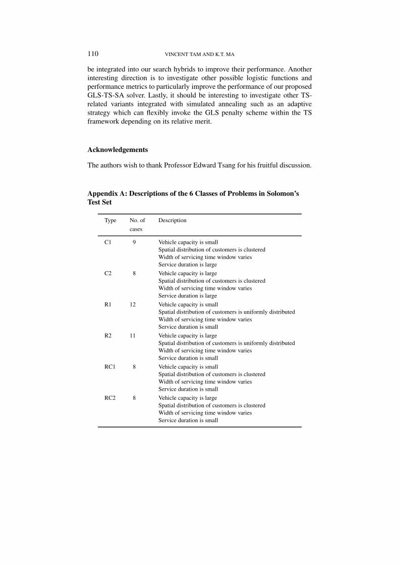
We used Solomon’s test cases to evaluate the performance of our proposalsagainst the original Tabu search (Gendreau et al. 1994) and Backer’s et al.’svariant – the Guided Tabu search (Backer et al. 1997). There are 56 instancesof delivery problems in the Solomon’s test set, each with 100 customers,which can be categorized into six classes: C1, C2, R1, R2, RC1 and RC2.The first letter(s) of the class name denotes the type of customer distribu-tion. For instance, ‘C’ represents the clustered customers, ‘R’ denotes therandomly distributed customers, and ‘RC’ involves a mix of customers ofboth types. After that, the number in the class name encodes the types ofvehicle capacity and service duration. ‘1’ refers to the test cases with smallvehicle capacity and short service duration while ‘2’ stands for those withlarge vehicle capacity and long service duration. For all the six classes,the demand for each customer within the same class is the same. Refer toAppendix A for the full description of each class.
The original guided local search (GLS) and Tabu search algorithms andtheir hybrids such as the guide Tabu search (GTS), our proposed guide localsearch – Tabu search (GLS-TS) and its variant GLS-TS integrated with simu-lated annealing (GLS-TS-SA) are all implemented in C/C++ and compiledwith g++ (the GNU C++ version egcs-2.91.66 with optimised compilationoption), running on a machine with Intel Pentium III (450Mhz) processorand 256 megabytes of random-access memory (RAM). The operating systemis Linux RedHat Version 6.1 (Cartman) Kernel 2.2.12–20 on i686. All theimplementations are in fact modified from the original PFIH+MGA (Jee2000). Most of the data structures are implemented as global arrays for effi-cient handling. Moreover, the four heuristic operators are modified so thatinstead of performing an actual move, the effects of performing the move arecalculated. This is achieved by considering the arcs added and deleted for aparticular move. For the constraint checking, the new move is only checkedagainst those routes it will affect. Hence, the execution time of the programis greatly reduced by a factor of 10 or more.
The lemma values used are 0.2 for GLS, and 0.15 for GTS, GLS-TS andGLS-TS-SA. For each approach, the solver is executed 10 times with theaverage and the best results recorded. For all the approaches, the resourcelimit or stopping criterion is set at 1000 iterations. For the following results,we use “PFIH+” to represent those search methods using the push-forwardinsertion heuristic for initialisation while “VVH+” is used to represent thosemethods using the virtual vehicle heuristic as discussed in Section 3.
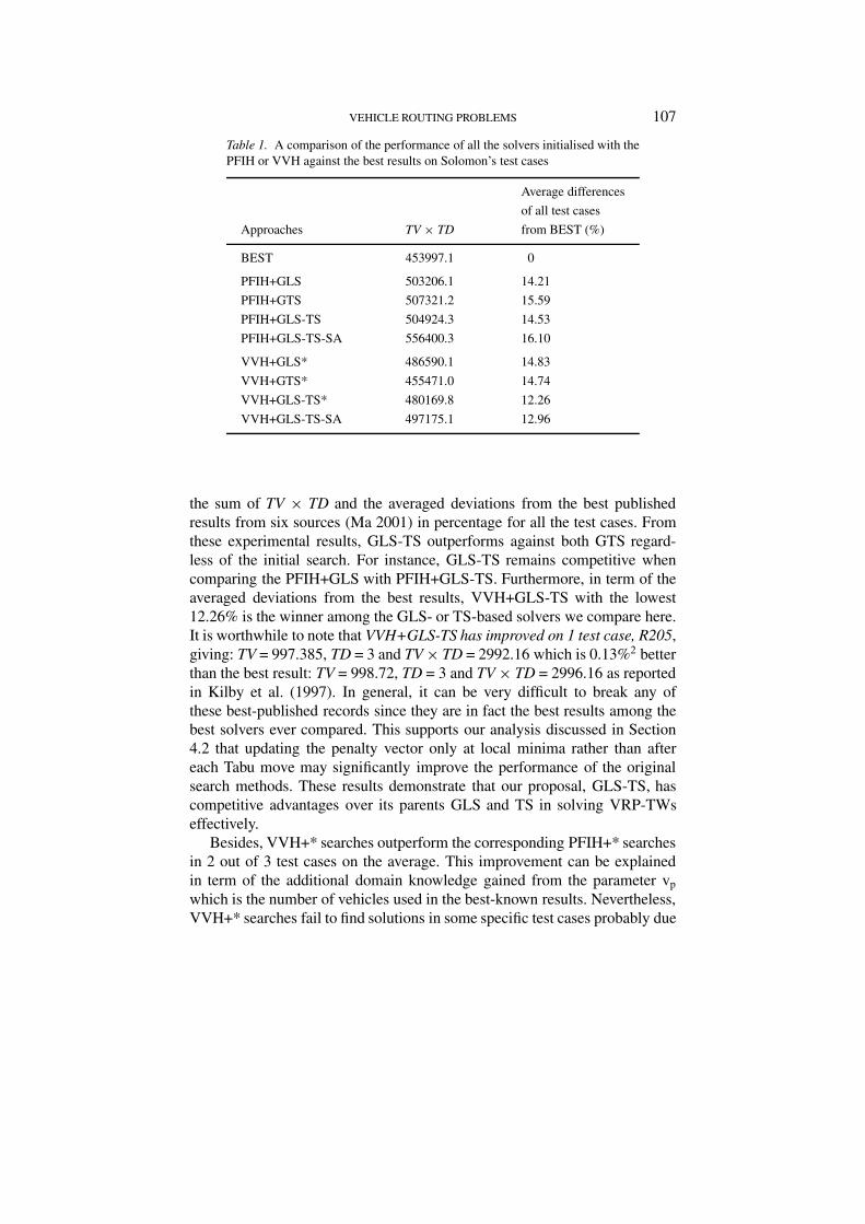
Table 1 summarizes the performance of different solvers initialised withPFIH or VVH in solving the Solomon’s test set (Solomon 1987) of VRP-TWs. The performance of the solvers is measured in terms of two quantities:
VEHICLE ROUTING PROBLEMS 107
Table 1. A comparison of the performance of all the solvers initialised with thePFIH or VVH against the best results on Solomon’s test cases
Average differences
of all test cases
Approaches TV × TD from BEST (%)
BEST 453997.1 0
PFIH+GLS 503206.1 14.21
PFIH+GTS 507321.2 15.59
PFIH+GLS-TS 504924.3 14.53
PFIH+GLS-TS-SA 556400.3 16.10
VVH+GLS* 486590.1 14.83
VVH+GTS* 455471.0 14.74
VVH+GLS-TS* 480169.8 12.26
VVH+GLS-TS-SA 497175.1 12.96
the sum of TV × TD and the averaged deviations from the best publishedresults from six sources (Ma 2001) in percentage for all the test cases. Fromthese experimental results, GLS-TS outperforms against both GTS regard-less of the initial search. For instance, GLS-TS remains competitive whencomparing the PFIH+GLS with PFIH+GLS-TS. Furthermore, in term of theaveraged deviations from the best results, VVH+GLS-TS with the lowest12.26% is the winner among the GLS- or TS-based solvers we compare here.It is worthwhile to note that VVH+GLS-TS has improved on 1 test case, R205,giving: TV = 997.385, TD = 3 and TV × TD = 2992.16 which is 0.13%2 betterthan the best result: TV = 998.72, TD = 3 and TV × TD = 2996.16 as reportedin Kilby et al. (1997). In general, it can be very difficult to break any ofthese best-published records since they are in fact the best results among thebest solvers ever compared. This supports our analysis discussed in Section4.2 that updating the penalty vector only at local minima rather than aftereach Tabu move may significantly improve the performance of the originalsearch methods. These results demonstrate that our proposal, GLS-TS, hascompetitive advantages over its parents GLS and TS in solving VRP-TWseffectively.
Besides, VVH+* searches outperform the corresponding PFIH+* searchesin 2 out of 3 test cases on the average. This improvement can be explainedin term of the additional domain knowledge gained from the parameter vp
which is the number of vehicles used in the best-known results. Nevertheless,VVH+* searches fail to find solutions in some specific test cases probably due
108 VINCENT TAM AND K.T. MA
to the bound vp + 1 or vp + 2 imposed on the initial search, which may hinderthe applicability of this initialisation heuristic in many real-life applications.After all, our proposed GLS-TS still proves to be effective with both PFIHand VVH.
In addition, VVH-GTS scored the lowest sum of TV × TD among thecompared solvers probably due to the probabilistic nature of the non-targetedstates, that are the non-X states as discussed in Section 4.2, which acciden-tally lead the search to the solution states in some specific instances. Theactual reason(s) for the overall improvement on the sum of TV × TD in thisparticular case require a more detailed investigation. Nevertheless, this resultclearly demonstrates the effectiveness of combining both GLS and TS meta-heuristics in solving real-life VRP-TWs.
Furthermore, the sum of TV × TD for the VVH+GLS-TS-SA is the largestamong the VVH+* solvers while the PFIH-GLS-TS-SA shows the largestaveraged deviations from the best results among all the comparing solvers,clearly demonstrating the difficulty in controlling the local search or Tabusearch with the integrated simulated annealing technique. We will try toexplain this difficulty in term of the probabilistic model we have discussedin Section 4.2. Roughly, integrating the simulated annealing technique todecide which search method to use in each iteration is similar to adding apre-requisite state before each original state in the state transitions of the TSalgorithm as shown in Figure 7(a). Each pre-requisite state has two out-goingarrows as two possible transitions – one leads to the original TS state whileanother leads to the additional local search state as possibly occurred in theGLS algorithm. The overall effect is the main component (pab·pbc·pcd ) of theprobability of successfully reaching the solution state is significantly loweredby a factor of hn where h, ranging from 0 to 1, is the probability of still beingthe most rewarding search method (with respect to the normal local searchmethod), and n is the number of TS states involved. Moreover, the newlyadded pre-requisite and local-search states into the original state transitiondiagram of the TS simply means the resulting GLS-TS-SA algorithm moredifficult to manage with more possibility to consider. After all, this observa-tion prompts us to carefully refine the simple performance measure used inour proposed GLS-TS-SA solver for testing.
Lastly, we try to identify the best optimiser for each of the 6 classes ofSolomon’s test cases. We observe for the C1 and C2 classes, where there isno clear winner in term of the sum of TV × TD, PFIH+GLS is the simplestand most stable solver. Also, it is worth noting that GLS-TS-SA is margin-ally better in the C1 class with only 0.14% deviated from the best publishedresults. In addition, VVH+GLS-TS performs the best for both R2 and RC2-type problems. For a more detailed comparison on the performance of the
VEHICLE ROUTING PROBLEMS 109
different solvers in each individual problem class of the Solomon’s test set,refer to (Ma 2001).
6. Concluding Remarks
In this paper, we proposed our 2 interesting search hybrids by integrating thewell-known guided local search (GLS) and Tabu search (TS) algorithms toeffectively solve the VRPs. As opposed to the GTS in (Backer et al. 1997),we consider a different integration of Tabu Search into GLS framework asGLS-TS in which the GLS-type penalty scheme is invoked only at stablestates. More interestingly, from GLS-TS, we implement the SA approachto work as the guiding principle to intelligently choose which is the rightsearch method to apply in each iteration based on some cooling schedules.The cooling schedule is governed by a standard logistic function as defined in(Spears 1993) together with some performance metric such as the reduction inthe total distance travelled. There was some previous work which combinedsimulated annealing with Tabu search (Spears 1993). However, in our work,the SA mechanism is embedded into the combined GLS and Tabu searchframework to decide which search method to apply in each search step.
In the empirical evaluation of our proposals on the Solomon’s bench-marks, we obtained exciting results from our proposed GLS-TS algorithm.Generally speaking, GLS-TS is a very efficient algorithm compared to itsancestors, the GLS and GTS. Surprisingly, the VV+GLS-TS produces abetter-than-best-published result for the R205 problem of the Solomon’s testset. In addition, from our empirical results, we made some careful observa-tions that improving on TV through any heuristic search operator can be morerewarding than the improvement on TD through the GLS-type penalty schemeon the long arcs since the objective function is TV × TD. This will definitelyprovide one exciting direction of our on-going research work. More impor-tantly, we provide in this paper a simple and interesting probabilistic modelfor analysing the search behaviour of our proposed hybrids. This readilyforms the basis for our future investigation.
Our new approach in the hybridisation of GLS and TS algorithms withsimulated annealing truly opens up many new directions for future explora-tion. Here, we suggest to use the simulated annealing as a more sophisticatedguiding principle, or namely meta-meta-heuristic, to monitor the underlyingmeta-heuristics such as GLS which in turn controls the search on the initialsolution returned by the initialisation heuristics such as the PFIH or VVH.As for future work, we should apply our proposed hybrid approaches tonew problem sets to demonstrate the best advantages of the different searchstrategies. Besides, we will look into other types of initialisation method to
110 VINCENT TAM AND K.T. MA
be integrated into our search hybrids to improve their performance. Anotherinteresting direction is to investigate other possible logistic functions andperformance metrics to particularly improve the performance of our proposedGLS-TS-SA solver. Lastly, it should be interesting to investigate other TS-related variants integrated with simulated annealing such as an adaptivestrategy which can flexibly invoke the GLS penalty scheme within the TSframework depending on its relative merit.
Acknowledgements
The authors wish to thank Professor Edward Tsang for his fruitful discussion.
Appendix A: Descriptions of the 6 Classes of Problems in Solomon’sTest Set
Type No. of Description
cases
C1 9 Vehicle capacity is smallSpatial distribution of customers is clusteredWidth of servicing time window variesService duration is large
C2 8 Vehicle capacity is largeSpatial distribution of customers is clusteredWidth of servicing time window variesService duration is large
R1 12 Vehicle capacity is smallSpatial distribution of customers is uniformly distributedWidth of servicing time window variesService duration is small
R2 11 Vehicle capacity is largeSpatial distribution of customers is uniformly distributedWidth of servicing time window variesService duration is small
RC1 8 Vehicle capacity is smallSpatial distribution of customers is clusteredWidth of servicing time window variesService duration is small
RC2 8 Vehicle capacity is largeSpatial distribution of customers is clusteredWidth of servicing time window variesService duration is small
VEHICLE ROUTING PROBLEMS 111
Notes
1. It should be noted that Solomon’s test cases (Solomon 1987) have been tackled byresearchers for decades, thus leaving very little room for improvement. Besides, theoriginal TS (Backer et al. 1997) and GLS (Tsang et al. 1999) methods already achievedrelatively good results as compared to the best published results. Thus, the averageimprovement of 1.7% on “long haul” problems is comparatively significant.
2. It should be noted that Solomon’s test cases (Solomon 1987) have been tackled byresearchers for decades, thus leaving little room for improvement. In addition, the originalTS (Backer et al. 1997) and GLS (Tsang et al. 1999) methods already achieved verygood results. Therefore, an improvement of 0.13% over the best published result can beimpressive and significant relative to the performance of all other solvers in the area.
References
De Backer, B., Furnon, V., Kilby, P., Prosser, P. & Shaw, P. (1997). Solving Vehicle RoutingProblems Using Constraint Programming and Met Heuristics. In Journal of Heuristics,Vol. 1–16. Kluwer Academic Publishers.
Gendreau, M., Hertz, A. & Laporte, G. (1994). A Tabu Search Heuristic for the VehicleRouting Problem. Management Science 40(10): 1276–1290.
Hoel, P. G. (1976). Elementary Statistics, 4th edn. John Wiley & Sons.Jee, J. C. (2000). Solving Vehicle Routing Problems with Time Windows Using Micro-Genetic
Algorithms. Proceedings of the 6th National Ungergraduate Research OpportunitiesProgramme Congress 2000. Faculty of Engineering, NUS, September 7–8.
Kilby, P., Prosser, P. & Shaw, P. (1997). Guided Local Search for the Vehicle Routing Prob-lems. In Proceedings of 2nd International Conference on Metaheuristics (MIC97), 1–10.Sophia-Antiplois, France, July 21–24.
Lin, S. (1965). Computer Solutions for the Traveling Salesman Problem. Bell SystemsTechnology Journal 44: 2245–2269.
Ma, K. T. (2001). Using Hybrid Search Methods to Solve A.I. Search and OptimizationProblems. Hons Thesis, The National University of Singapore.
Osman, I. H. (1993). Metastrategy Simulated Annealing and Tabu Search Algorithms for theVehicle Routing Problem. Ann. Oper. Res. 41: 421–451.
Prosser, P. & Shaw, P. (1997). Study of Greedy Search with Multiple Improvement Heuristicsfor Vehicle Routing Problems. Technical Report RR/96/201, Department of ComputerScience, Univeristy of Strathclyde, Glasgow.
Rochat, Y. & Taillard, E. D. (1995). Probabilistic Diversification and Intensification in LocalSearch for Vehicle Routing. Technical Report CRT-95-13, Centre de recherche sur lestransports, Université de Montréal, Montréal.
Savelsbergh, M. W. P. (1988). Computer Aided Routing. Amsterdam: Centrum voor Wiskundeen Informatica.
Seah, D. (1999). Ant Colonoy Optimization On Vehicle Routing Problems. Thesis for theMaster of Computer Science, National University of Singapore.
Solomon, M. M. (1987). Algorithms for the Vehicle Routing and Scheduling Problem withTime Windows. Oper. Res. 35: 254–265.
Spears, W. M. (1993). Simulated Annealing for Hard Satisfiability Problems. NCARAI Tech.Report AIC 93-015. AI Center, Naval Research Laboratory, Washington D.C.
112 VINCENT TAM AND K.T. MA
Tsang, E., Wang, C. J., Davenport, A., Voudouris, C. & Tung, L. L. (1999). A Familyof Stochastic Methods for Constraint Satisfaction and Optimisation. The First Interna-tional Conference on the Practical Application of Constraint Technologies and LogicProgramming. London.
Voudouris, C. & Tsang, E. (1995). Technical Report CSM-247. Department of ComputerScience, Univeristy of Essex.
Wah, B. & Chen, Y. X. (2000). Constrained Genetic Algorithms and Their Applications inNonlinear Constrained Optimization. Proceedings of IEEE ICTAI. Vancouver, Canada.