Embed Size (px)
Citation preview

Combining Iterated Local Search and Biased Randomization for solving non-smooth flow-
shop problems
IEMAE
Albert Ferrer, Angel A. Juan, Helena R. Lourenço
Dep. Applied Mathematics I
Universitat Politécnica de Catalunya, SPAIN

1. Convex Optimization Problems (COPs)
2. Non-Convex Optimization Problems (NCOPs)
3. Non-Smooth Optimization Problems (NSPs)
4. The Flow-Shop problem (Makespan)
5. The NEH heuristic for FSP
6. The ILS-ESP algorithm for FSP
7. Randomizing Classical Heuristics
8. A More Realistic Model for FSP (Tardiness)
9. Conclusions and Future Work
Overview

1. Convex Optimization Problems (COPs)
COPs are problems where all of the constraints are convex functions, and the objective is a convex function if minimizing, or a concave function if maximizing.
Linear functions are convex, so LP problems are COPs.
In a COP, the feasible region –the
intersection of convex constraint functions– is also a convex region.
With a convex objective and a convex feasible region, each optimal solution is globally optimal. Several methods –e.g. Interior Point methods– will either find the globally optimal solution, or prove that there is no feasible solution to the problem.
COPs can be solved efficiently up to very large size.
A convex functionA convex function
LPs are COPsLPs are COPs
A convex regionA convex region
Source: www.solver.com
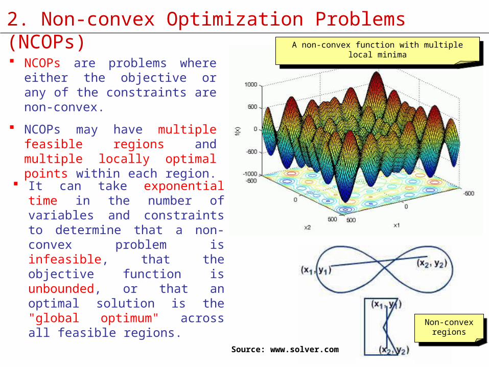
2. Non-convex Optimization Problems (NCOPs)
NCOPs are problems where either the objective or any of the constraints are non-convex.
NCOPs may have multiple feasible regions and multiple locally optimal points within each region.
It can take exponential time in the number of variables and constraints to determine that a non-convex problem is infeasible, that the objective function is unbounded, or that an optimal solution is the "global optimum" across all feasible regions.
Non-convex regions
Non-convex regions
Source: www.solver.com
A non-convex function with multiple local minimaA non-convex function with multiple local minima

3. Non-Smooth Optimization Problems (NSPs) Typically, NSPs are also NCOPs. Hence:
They might have multiple feasible regions and multiple locally optimal points within each region –because some of the functions are non-smooth or even discontinuous, and
Derivative/gradient information generally cannot be used to determine the direction in which the function is increasing (or decreasing).
In a NSP, the situation at one possible solution gives very little information about where to look for a better solution.
In most NSPs it is impractical to enumerate all of the possible solutions and obtain the best one. Hence, most methods rely on some sort of random sampling of possible solutions.
Such methods are nondeterministic or stochastic –they may yield different solutions on different runs, depending on which points are randomly sampled.
Examples of non-smooth functionsExamples of non-smooth functions
Source: www.mathworks.com

3. Examples of Nonsmooth Functions
Sensor Network Localization
The Problem The objective function
Optimal Circuit Routing
Winner Determination Problem
4. The Flow-Shop problem (1/2)
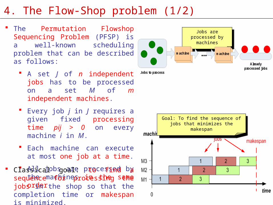
The Permutation Flowshop Sequencing Problem (PFSP) is a well-known scheduling problem that can be described as follows:
A set J of n independent jobs has to be processed on a set M of m independent machines.
Every job j in J requires a given fixed processing time pij > 0 on every machine i in M.
Each machine can execute at most one job at a time.
All jobs are processed by the machines in the same order.
Classical goal: to find a sequence for processing the jobs in the shop so that the completion time or makespan is minimized.
Jobs are processed by machines
Jobs are processed by machines
Goal: To find the sequence of jobs that minimizes the makespan
Goal: To find the sequence of jobs that minimizes the makespan
machine ...
Jobs to process
Already processed jobs
machine

4. The Flow-Shop problem (2/2)
The PFSP is a combinatorial problem with n! possible sequences which, in general, is NP-complete.
A large number of different approaches have been developed: from pure optimization methods (e.g. mixed integer programming) to the use of heuristics and metaheuristics.
Still, there is a need for new efficient, simple and parameter-free (ESP) methods able to provide a large set of alternative near-optimal solutions with different properties, so that decision-makers can choose among different alternative solutions according to their specific necessities and preferences.
MetaheuristicsMetaheuristics
Utility functionUtility function

5. The NEH heuristic (Nawaz et al. 1983)
Calculate the total processing time required for each job, and then to create an “efficiency list” of jobs sorted in a descending order
NEH is probably the most efficient heuristic for the PFSPNEH is probably the most efficient heuristic for the PFSP
At each step, the job at the top of the efficiency list is selected and used to construct the solution.
Once selected, a job is inserted in the sorted set of jobs that are configuring the ongoing solution. The exact position that the selected job will occupy in that ongoing solution is given by the minimizing makespan criterion.
Job 1
Job 2
Job n
…
Job i For each job, calculate its total processing time
Construct a sorted efficiency list
(jobs with higher processing times at the top)
At each iteration, select the job at the top of the list
Job 1 Job 2
Job 3Each new job is inserted into the “best” possible position

6. The ILS-ESP algorithm The ILS-ESP is based
on the IG-ILS (Ruiz 2007). It is equally Efficient, Simpler and Parameter-free.
It incorporates 3 major changes with respect to IG-ILS: (1) the RandNEH method, which provides diversification in the initial solution, (2) a new ‘enhanced swap’ operator, and (3) a simpler Demon-based acceptance criterion.
ILS-ESP is an efficient, simple and parameter-free algorithm for the PFSPILS-ESP is an efficient, simple and parameter-free algorithm for the PFSP
We have tested ILS-ESP vs. IG-ILS using the Taillard benchmarks (120 instances) and they seem to offer equivalent performance: Average GAP = 0.36% in 10ms*nJobs*nMachines and after running each algorithm 10 times (replicas).
Iterated Local Search frameworkIterated Local Search framework
Randomized NEH solutionRandomized NEH solution
Enhanced Swap operatorEnhanced Swap operator
Demon-like acceptance criterionDemon-like acceptance criterion
0 parameters0 parameters
50403020100
0.20
0.15
0.10
0.05
0.00
X
Pro
bability
0.10.2
p
Distribution PlotGeometric
X = total number of trials.
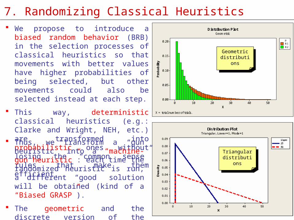
7. Randomizing Classical Heuristics We propose to introduce a biased
random behavior (BRB) in the selection processes of classical heuristics so that movements with better values have higher probabilities of being selected, but other movements could also be selected instead at each step.
This way, deterministic classical heuristics (e.g.: Clarke and Wright, NEH, etc.) are transformed into probabilistic ones without losing the “common sense” rules that make them efficient.
Thus, we transform a “gun heuristic” into a “machine-gun heuristic”: each time the randomized heuristic is run, a different “good” solution will be obtained (kind of a “Biased GRASP”).
The geometric and the discrete version of the triangular can be used to infer this BRB.
Geometric distributions
Geometric distributions
Triangular distributions
Triangular distributions

NEH jobs are ordered in decreasing order according to their total completion time on all the machines
RandNEH introduces randomness in this process by using a triangular statistical distribution jobs that take longer to complete will be more likely to be selected first, but all jobs in the list are potentially eligible.
8. RandNEH: Randomizing the NEH for the PFSP
1817161514131211109876543210
600
500
400
300
200
100
0
C2
Count
Chart of C2
Notice: Each time RandNEH is run, a different random solution is obtained. By construction, chances are that this solution outperforms the NEH one and, in any case, this solution will be a good alternative to the original NEH diversification of the starting base solution.
Generating triangular random variates• Calculate u ~ U(0,1)• Calculate X = b * (1 – Sqrt(1 – u))• Calculate pos = Floor(X)
Generating triangular random variates• Calculate u ~ U(0,1)• Calculate X = b * (1 – Sqrt(1 – u))• Calculate pos = Floor(X)

9. The Enhanced Swap & the Acceptance CriterionNew Enhanced Swap operator:1. Select two positions at
random.2. Interchange jobs at the
selected positions.3. Perform a sorted ‘shift-to-
left’ movement to ‘adjust’ the positions of the swapped jobs.
New Enhanced Swap operator:1. Select two positions at
random.2. Interchange jobs at the
selected positions.3. Perform a sorted ‘shift-to-
left’ movement to ‘adjust’ the positions of the swapped jobs.
New acceptance criterion:1. If the new solution improves the best
solution, then update base solution (improvement).
2. Else, accept the new solution as the base solution (degeneration) as far as the last movement was an improvement and the degeneration is not greater than the last improvement.
New acceptance criterion:1. If the new solution improves the best
solution, then update base solution (improvement).
2. Else, accept the new solution as the base solution (degeneration) as far as the last movement was an improvement and the degeneration is not greater than the last improvement.

1. Test: 15 runs per instance with maxTime = 0.010s * nJobs * nMachines
2. Computer: Intel Xeon 2.0GHz 4GB RAM
3. Note: All algorithms have been implemented in Java (non-optimized code)
10. The Flow-Shop Problem: Some results
Juan, A.; Ruiz, R.; Mateo, M.; Lourenço, H.; Ionescu, D. (2010): “A Simulation-based Approach for Solving the Flowshop Problem”. In Proceedings of the 2010 Winter Simulation Conference.
Juan, A.; Ruiz, R.; Mateo, M.; Lourenço, H.; Ionescu, D. (2010): “A Simulation-based Approach for Solving the Flowshop Problem”. In Proceedings of the 2010 Winter Simulation Conference.

11. FSP: A More Realistic Model
The following notation is used for the description of the flow-shop problem:

12. FSP: Objective Function

13. FSP: The Model
14. FSP in production industries
1. Most of the flow-shop problems arise in production industries, where a set of products or jobs must be produced.

14. FSP in production industries
1. Most of the flow-shop problems arise in production industries, where a set of products or jobs must be produced.
2. These industries usually are integrated in a supply chain, meaning that after being produced they are transported to a warehouse or customers.

14. FSP in production industries
1. Most of the flow-shop problems arise in production industries, where a set of products or jobs must be produced.
2. These industries usually are integrated in a supply chain, meaning that after being produced they are transported to a warehouse or customers.
3. Usually this transportation is set in advance and it has a periodicity, for example every 2 hours or morning and afternoon.
4. In this case the due date is related with this transportation schedule, a job is produced on time if it can meet its transportation due date, and if it late the jobs must be scheduled to later transport.

15. FSP transportation scheduled
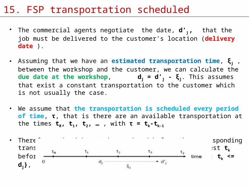
• The commercial agents negotiate the date, d’j, that the job must be delivered to the customer's location (delivery date ).

15. FSP transportation scheduled
• The commercial agents negotiate the date, d’j, that the job must be delivered to the customer's location (delivery date ).
• Assuming that we have an estimated transportation time, ξj , between the workshop and the customer, we can calculate the due date at the workshop, dj = d’j - ξj. This assumes that exist a constant transportation to the customer which is not usually the case.
• We assume that the transportation is scheduled every period of time, τ, that is there are an available transportation at the times t0, t1, t2, … , with τ = tk-tk-1
• Therefore, the job must be produced before the corresponding transportation schedule time, tk
j, which is the closest tk before the workshop due date dj, tk
j= max{ tk : tk <= dj}, otherwise the job can not arrive on time.
16. FSP penalizationsDifferent situations can occur:

16. FSP penalizationsDifferent situations can occur:
The job is completed on time, just before the correspondent transportation schedule,
tkj - τ < Cm,j <= tk
j,
after being produced the jobs goes directly to the vehicle, and it is on time to me delivered to the customer; so, there is no penalization for being early or late..
The job is completed too early, i.e., before the previous correspondent transportation schedule,
Cm,j <= tkj - τ,
therefore the company has to store this job on a warehouse so there exist a penalization related with the time that the product or job must be stored in the workshop. This cost makes sense, since today most of the production companies have limited storing space.
The job is completed too late, i.e. after the correspondent transportation schedule,
Cm,j > tkj ,
therefore the job miss its corresponding transportation and it will be delivered late. In this case we propose to types of penalization, by the time that the job is late and by the number of periods that it is late.

16. FSP penalizationsDifferent situations can occur:
The job is completed on time, just before the correspondent transportation schedule,
tkj - τ < Cm,j <= tk
j,
after being produced the jobs goes directly to the vehicle, and it is on time to me delivered to the customer; so, there is no penalization for being early or late..
The job is completed too early, i.e., before the previous correspondent transportation schedule,
Cm,j <= tkj - τ,
therefore the company has to store this job on a warehouse so there exist a penalization related with the time that the product or job must be stored in the workshop. This cost makes sense, since today most of the production companies have limited storing space.
The job is completed too late, i.e. after the correspondent transportation schedule,
Cm,j > tkj ,
therefore the job miss its corresponding transportation and it will be delivered late. In this case we propose two types of penalization, by the time that the job is late and by the number of periods that it is late.
17. FSP: Earliness and Tardiness
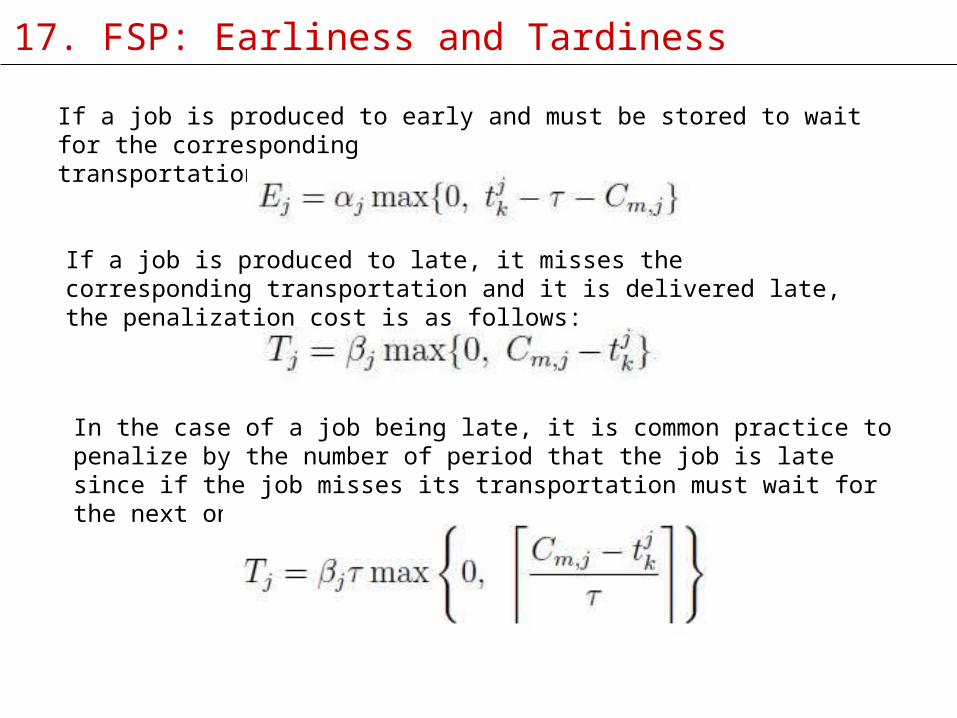
If a job is produced to early and must be stored to wait for the correspondingtransportation we have the following cost:
If a job is produced to late, it misses the corresponding transportation and it is delivered late, the penalization cost is as follows:
In the case of a job being late, it is common practice to penalize by the number of period that the job is late since if the job misses its transportation must wait for the next one.

18. Conclusions & Future Work
We have discussed the use of probabilistic or stochastic algorithms for solving non-smooth combinatorial optimization problems in the case of FSP.

18. Conclusions & Future Work
We have discussed the use of probabilistic or stochastic algorithms for solving non-smooth combinatorial optimization problems in the case of FSP.
We propose the use of probability distributions, such as the Triangular one, to add a biased random behavior to classical NEH heuristic for the Flow Shop Scheduling Problem.
By randomizing these heuristic, a large set of alternative good solutions can be quickly obtained in a natural and easy way.
Some specific example in the makespan version of this technique have been analyzed to illustrate the main ideas behind this approach.
An extension of the FSP that includes intermediary inventory holding cost and the sum of earliness and tardiness has been described in order to present a more realistic model (in progress).

Combining Iterated Local Search and Biased Randomization for solving non-smooth flow-
shop problems
IEMAE
Albert Ferrer, Angel A. Juan, Helena R. Lourenço
Dep. Applied Mathematics I
Universitat Politécnica de Catalunya, SPAIN
Thank You!Thank You!