Embed Size (px)
Citation preview
Combining freeform optics and curved detectors for wide field imaging: a polynomial approach over squared aperture
EDUARD MUSLIMOV,1,2,* EMMANUEL HUGOT,1 WILFRIED JAHN,1 SEBASTIEN
VIVES,1 MARC FERRARI,1 BERTRAND CHAMBION,3 DAVID HENRY3 AND
CHRISTOPHE GASCHET1,3 1Aix Marseille Univ, CNRS, LAM, Laboratoire d'Astrophysique de Marseille, 38, rue Joliot-Curie,
Marseille,13388, France 2Kazan National Research Technical University named after A.N. Tupolev –KAI, 10 K. Marx, Kazan
420111, Russian Federation 3Univ. Grenoble Alpes, CEA, LETI, MINATEC campus, F38054 Grenoble, France
Abstract:. In the recent years a significant progress was achieved in the field of design and
fabrication of optical systems based on freeform optical surfaces. They provide a possibility to
build fast, wide-angle and high-resolution systems, which are very compact and free of
obscuration. However, the field of freeform surfaces design techniques still remains
underexplored. In the present paper we use the mathematical apparatus of orthogonal
polynomials defined over a square aperture, which was developed before for the tasks of
wavefront reconstruction, to describe shape of a mirror surface. Two cases, namely Legendre
polynomials and generalization of the Zernike polynomials on a square, are considered. The
potential advantages of these polynomials sets are demonstrated on example of a three-mirror
unobscured telescope with F/#=2.5 and FoV=7.2x7.2°. In addition, we discuss possibility of
use of curved detectors in such a design.
OCIS codes: (110.6770) Telescopes, (080.4228) Nonspherical mirror surfaces, (080.4035) Mirror system design,
(040.1520) CCD, charge-coupled device.
References and links
1. T. Yang, J. Zhu, X. Wu and G. Jin, “Direct design of freeform surfaces and freeform imaging systems with a
point-by-point three-dimensional construction-iteration method,” Opt. Express 23, 10233-10246 (2015). 2. Q. Meng, H. Wang, K. Wang, Y. Wang, Zh. Ji and Dong Wang, “Off-axis three-mirror freeform telescope with
a large linear field of view based on an integration mirror,” Appl. Opt. 55, 8962-8970 (2016).
3. Q. Meng, W. Wang, H. Ma and J. Dong, “Easy-aligned off-axis three-mirror system with wide field of view using freeform surface based on integration of primary and tertiary mirror,” Appl. Opt. 53, 3028-3034 (2014).
4. J. Zhu, W. Hou, X. Zhang and G. Jin, “Design of a low F-number freeform off-axis three-mirror system with
rectangular field-of-view,” Journal of Optics 17(1), 015605 (2015). 5. S. Gautam, A. Gupta and G. Singh, “Optical design of off-axis Cassegrain telescope using freeform surface at
the secondary mirror,” Opt. Eng. 54(2),025113 (2015).
6. S.. Kim , S., S. Chang, S. Pak, K. J. Lee, B. Jeong, G.-J. Lee, G. H. Kim, S. K. Shin and S. M. Yoo, “Fabrication of electroless nickel plated aluminum freeform mirror for an infrared off-axis telescope,” Appl.
Opt. 54, 10137-10144 (2015).
7. A. Hofmann, J. Unterhinninghofen, H. Ries and S. Kaiser, “Double tailoring of freeform surfaces for off-axis aplanatic systems,” Proc. SPIE 8550, 855014 (2012).
8. K. Fuerschbach, G.E. Davis, K.P. Thompson and J.P. Rolland, “Assembly of a freeform off-axis optical system
employing three φ-polynomial Zernike mirrors,” Opt. Lett. 39, 2896-2899 (2014). 9. E. Hugot, X. Wang, D. Valls-Gabaud, G.R. Lemaître, T. Agócs, Rong Shu and J. Wang, “A freeform-based,
fast, wide-field, and distortion-free camera for ultralow surface brightness surveys,” Proc. SPIE 9143, 91434X
(2014). 10. M.P. Chrisp, B. Primeau and M.A. Echter, “Imaging freeform optical systems designed with nurbs surfaces,”
Opt. Eng. 55(7),071208 (2016).
11. M. P. Chrisp, “New freeform NURBS imaging design code,” Proc. SPIE. 9293, 92930N (2014).

12. M.P. Chrisp, “Three Mirror Anastigmat Designed with NURBS Freeform Surfaces,” in Renewable Energy and
the Environment: Postdeadline Papers, OSA Postdeadline Paper Digest (online) (Optical Society of America, 2013), paper FM4B.3.
13. S. Pascal, M. Gray, S. Vives, D. Le Mignant, M. Ferrari, J.-G. Cuby and K. Dohlen, “New modelling of
freeform surfaces for optical design of astronomical instruments,” Proc. SPIE 8450, 845053 (2012). 14. M. Nikolic, P. Benítez, B. Narasimhan, D. Grabovickic, J. Liu and J.C. Miñano, “Optical design through
optimization for rectangular apertures using freeform orthogonal polynomials: a case study,” Opt. Eng.
55(7),071204 (2016). 15. M. Rossi, G. Borghi, I.A. Neil, G. Valsecchi, P. Zago and F.E. Zocchi, “Electroformed off-axis toroidal
aspheric three-mirror anastigmat multispectral imaging system,” Opt. Eng. 53(3), 031308 (2014).
16. C. Menke and G.W. Forbes,”Optical design with orthogonal representations of rotationally symmetric and freeform aspheres,” Advanced Optical Technologies 2(1), 97-109 (2013).
17. M. Maksimovic, “Optical design and tolerancing of freeform surfaces using anisotropic radial basis functions,”
Opt. Eng. 55(7), 071203 (2016). 18. R.N. Youngworth and E.I. Betensky, “Lens design with Forbes aspheres,” Proc. SPIE 7100, 71000W (2008).
19. M. Nikolic, P. Benítez, J. C. Miña, D. Grabovickic, J. Liu, B. Narasimhn and M. Buljan, “Optical design
through optimization using freeform orthogonal polynomials for rectangular apertures,” Proc. SPIE 9626, 96260V (2015).
20. J. Ye, Zh. Gao, Sh. Wang, J. Cheng, W. Wang and W. Sun, “Comparative assessment of orthogonal
polynomials for wavefront reconstruction over the square aperture,” J. Opt. Soc. Am. A 31, 2304-2311 (2014). 21. T. M. Apostol, Linear Algebra: A First Course, with Applications to Differential Equations (Wiley, 1997).
22. R.Upton and B. Ellerbroek, “Gram-Schmidt orthogonalization of the Zernike polynomials on apertures of
arbitrary shape,” Opt. Lett. 29, 2840–2842 (2004). 23. K. Fuerschbach, J.P.Rolland and K.P.Thompson, “A new family of optical systems employing φ-polynomial
surfaces,” Opt. Express 19, 21919-21928 (2011).
24. U.Fuchs and S.R. Kiontke, “Discussing design for manufacturability for two freeform imaging systems,” Proc. SPIE 9948, 99480L (2016).
25. R. Hentschel, B. Braunecker and H.J. Tiziani Advanced Optics Using Aspherical Elements (SPIE Publishing, 2008).
26. P. K. Swain, D. J. Channin, G. C. Taylor, S. A. Lipp and D. S. Mark, “Curved ccds and their application with
astronomical telescopes and stereo panoramic cameras,” Proc. SPIE 5301, 109–129 (2004). 27. S.-B.Rim, P. B. Catrysse, R. Dinyari K., Huang and P.Peumans, “The optical advantages of curved focal plane
arrays,” Opt. Express, 16, 4965–4971 (2008).
28. R.Dinyari, S.-B. Rim, K. Huang, P. B. Catrysse and P. Peumans, “Curving monolithic silicon for nonplanar focal plane array applications,” Applied Physics Letters, 92(9), (2008).
29. M. P. Lesser and J. A. Tyson, “Focal Plane Technologies for LSST,” Proc. SPIE 4836, 240 (2002).
30. S.Nikzad, M. Hoenk and T. Jones, “Solid-state curved focal plane arrays,” (2010). US Patent 7,786,421.
31. O.Iwert, D.Ouellette, M.Lesser and B.Delabre, “First results from a novel curving process for large area
scientific imagers,” Proc. SPIE 8453, 84531W (2012).
32. M. Ferrari, “Development of a variable curvature mirror for the delay lines of the VLT interferometer,” Astronomy & Astrophysic, suppl. Ser. 128, 221–227 (1998).
33. B.Chambion, L. Nikitushkina, Y. Gaeremynck, W. Jahn, E. Hugot, G. Moulin, S. Getin, A. Vandeneynde, and
D. Henry, “Tunable curvature of large visible CMOS image sensors: Towards new optical functions and system miniaturization,” in Proceedings of IEEE 66th Electronic Components and Technology Conference (IEEE,
2016), pp.178- 187.
34. E. Hugot, G.R.Lemaitre and M. Ferrari, “Active optics: single actuator principle and angular thickness distribution for astigmatism compensation by elasticity”, Applied Optics 47, 10, (2008).
35. M. Laslandes, E. Hugot, M. Ferrari, C. Hourtoule, C. Singer, C. Devilliers, C. Lopez and F. Chazallet, “Mirror
actively deformed and regulated for applications in space: design and performance,” Opt. Eng. 52(9), 091803 (2013).
36. B. Guenter, N. Joshi, R. Stoakley, A. Keefe, K. Geary, R. Freeman, J. Hundley, P. Patterson, D. Hammon, G.
Herrera, E. Sherman, A. Nowak, R. Schubert, P. Brewer, L. Yang, R. Mott and G. McKnight, “Highly curved image sensors: a practical approach for improved optical performance,” Opt. Express 25, 13010-13023 (2017).
37. J. M. Geary, Introduction to Lens Design: With Practical Zemax Examples (Willmann-Bell, 2002).
1. Introduction
Freeform optical surfaces open a new window for optical design of innovative systems. There
is a constantly growing number of examples demonstrating that use of freeform surfaces allows
to build imaging systems with improved resolution across an increased field of view together
with a larger aperture. These examples spread over different application fields and use different
approaches to describe the freeform surfaces.
In the current study we focus on all-reflective unobscured telescope systems, which utilize
freeform mirrors. We also put a special accent on applications requiring high performance like
astronomy and astrophysics. The latter condition implies that we put more accent on solutions
with medium-to-high apertures and high resolution.
Comparing the existing designs in the specified area, one can see that the majority of the
published solutions can be classified as unobscured TMA-type telescopes, while other types
like derivatives from Cassegrain or Schwarzchild designs with two mirrors or SEAL-type
designs with four mirrors are rarer.
In the considered examples a few mathematical descriptions of the freeform surfaces are
applied: ordinary XY-polynomials [1-7], Zernike polynomials [8, 9], non-uniform rational B-
splines (NURBS) [10-12] and a few other types of equations, used in [13-17]. Among the latter
it is reasonable to note Bernstein polynomials [13] and Legendre/Q-Legendre polynomials [14].
This overview is not absolutely exhaustive, but it represents the variety of existing approaches
to freeform design.
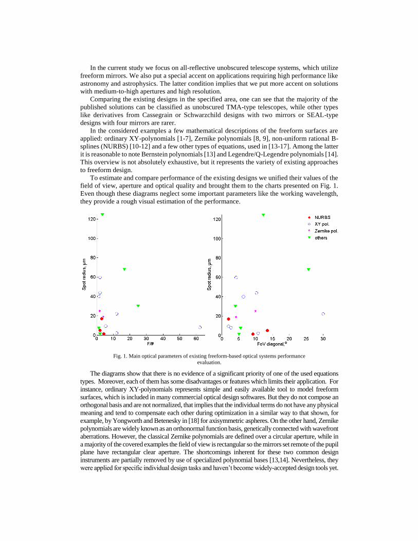
To estimate and compare performance of the existing designs we unified their values of the
field of view, aperture and optical quality and brought them to the charts presented on Fig. 1.
Even though these diagrams neglect some important parameters like the working wavelength,
they provide a rough visual estimation of the performance.
Fig. 1. Main optical parameters of existing freeform-based optical systems performance
evaluation.
The diagrams show that there is no evidence of a significant priority of one of the used equations
types. Moreover, each of them has some disadvantages or features which limits their application. For
instance, ordinary XY-polynomials represents simple and easily available tool to model freeform
surfaces, which is included in many commercial optical design softwares. But they do not compose an
orthogonal basis and are not normalized, that implies that the individual terms do not have any physical
meaning and tend to compensate each other during optimization in a similar way to that shown, for
example, by Yongworth and Betenesky in [18] for axisymmetric aspheres. On the other hand, Zernike
polynomials are widely known as an orthonormal function basis, genetically connected with wavefront
aberrations. However, the classical Zernike polynomials are defined over a circular aperture, while in
a majority of the covered examples the field of view is rectangular so the mirrors set remote of the pupil
plane have rectangular clear aperture. The shortcomings inherent for these two common design
instruments are partially removed by use of specialized polynomial bases [13,14]. Nevertheless, they
were applied for specific individual design tasks and haven’t become widely-accepted design tools yet.
For instance, it was shown that use of Q-Legendre polynomials allows to cover a huge field of view
up to 51.4° [19], but the values of aperture and resolution achieved there makes the design incompatible
with the most of optical systems used in astronomy. Finally, the NURBS-based designs shown some
promising results, but they are based on a finite grid of points, that complicates their optimization with
existing means. Thus we can conclude that in spite of fast progress of the freeform optics the questions
of their mathematical description still remains underexplored.
Thus it is very desirable to describe freeform surfaces by such an equation, which would be
defined over a square aperture, easily realizable in current optical design software and
consistent with existing optimization techniques. The primary goal of this paper is to find such
sets of equations and demonstrate their advantages for design of a high-aperture wide-field
unobscured reflective telescope.
In the field of wavefront reconstruction and analysis similar problem was solved in a few
different ways and this adjacent field can propose a number of mathematical approaches to the
surface definition. Paper [20] describes use of Legendre polynomials and Zernike polynomials
generalized for a case of square aperture for wavefront reconstruction. In the present study we
consider possibility of their application to design of freeform mirrors. We briefly discuss their
features and transform them for use in a ray-tracing code. Further we apply them for design of
a fast wide-field TMA-type unobscured telescope and analyze the found design solutions.
2. The polynomial bases
In the current study we use the same definition of the 2D Legendre polynomials as that used in
[20]. They are orthonormal over the unit square aperture and can be easily derived from 1D
Legendre polynomials. However, we consider to be useful to present here a table of the
polynomials written in explicit from. Firstly, it is convenient for composing a code for ray-
tracing, and secondly, it is necessary for making cross-check with ordinary XY-polynomials,
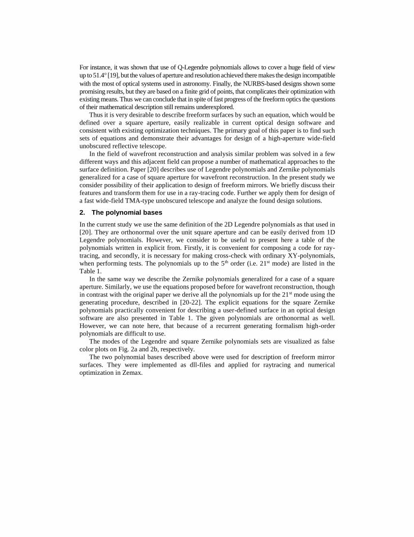
when performing tests. The polynomials up to the 5th order (i.e. 21st mode) are listed in the
Table 1.
In the same way we describe the Zernike polynomials generalized for a case of a square
aperture. Similarly, we use the equations proposed before for wavefront reconstruction, though
in contrast with the original paper we derive all the polynomials up for the 21st mode using the
generating procedure, described in [20-22]. The explicit equations for the square Zernike
polynomials practically convenient for describing a user-defined surface in an optical design
software are also presented in Table 1. The given polynomials are orthonormal as well.
However, we can note here, that because of a recurrent generating formalism high-order
polynomials are difficult to use.
The modes of the Legendre and square Zernike polynomials sets are visualized as false
color plots on Fig. 2a and 2b, respectively.
The two polynomial bases described above were used for description of freeform mirror
surfaces. They were implemented as dll-files and applied for raytracing and numerical
optimization in Zemax.
Table 1. Explicit form of the 2D Legendre and square Zernike polynomials
Mode
number, k
Lk(x,y) Sk(x,y)
1 1 1
2 1.7321·x 1.7321·x
3 1.7321·y 1.7321·y
4 3.3541·x2-1.1180 2.3717·x2+2.3717·y2-1.5811
5 3·xy 3·xy
6 3.3541·y2-1.1180 2.3717·x2-2.3717·y2
7 6.6144·x3-3.9686·x 4.3649·x2y+4.3649·y3-4.0739·y
8 5.8095·x2y-1.9365·y 4.3649·x3+4.3649·xy2-4.0739·x
9 5.8095·xy2-1.9365·x 3.8337·x2y-4.9697·y3+1.7039·y
10 6.6144·y3-3.9686·y 4.9697·x3-3.8337·xy2-1.7039·x
11 13.125·x4-11.25·x2+1.125 4.8104·x4+9.6208·x2y2+4.8104·y4-7.3302·x2
-7.3302·y2+1.8936
12 11.4564·x3y-6.8739·xy 9.2808·x4-7.9550·x2-9.2808·y4+7.9550·y2
13 11.25·x2y2-3.75·x2-3.75·y2+1.25 8.1009·x3y+8.1009·xy3-9.7211·xy
14 11.4564·xy3-6.8739·xy 7.9368·x4-5.8311·x2y2+7.9368·y4-4.8593·x2
-4.8593·y2+0.7127
15 13.125·x4-11.25·x2+1.125 8.1009·x3y-8.1009·xy3
16 26.1184x5-29.0205x3+6.2187x -18.5336·x4-11.2976·y4-35.1004·x2y2+19.1136·x2+
13.9594·y2+6.5222·x5+13.0443·x3y2+6.5222·xy4
-7.8266·xy2-7.8266·x3+1.9567·x-3.0410
17 22.7332·x4y-19.4856·x2y+1.9486·y 16.9179·xy-19.1009·x3y-24.2833·xy3
-5.1293·y5+10.2585·x2y3 +5.1293·x4y
-6.1551·y3-6.1551·x2y+1.5388·y
18 22.1853·x3y2-7.3951·x3-13.3112·xy2+4.4371·x -16.0381·x4+16.6285·y4+8.3475·x2y2+11.5745·x2
-12.7060·y2+9.4550·x5-0.1453·x3y2-9.6003·xy4
+5.8038·xy2-9.4405·x3+1.4074·x-0.3713
19 22.1853·x2y3-7.3951·y3-13.3112·x2y+4.4371·y 10.9852·xy-22.10429·x3y-5.4609·xy3
-4.9216·y5+3.9945·x2y3 +8.9161·x4y
+4.5222·y3-6.5480·x2y-0.4387·y
20 22.7332·xy4-19.4856·xy2+1.9486·x -6.7585·x4-10.4893·y4+10.4171·x2y2+4.8521·x2
+5.1792·y2+7.5073·x5-6.8079·x3y2+6.0569·xy4
-1.5917·xy2-6.8265·x3+1.3795·x-1.0772
21 26.1184·y5-29.0205·y3+6.2187·y -1.0178·xy-7.5887·x3y+11.6480·xy3
2.3698·y5-6.2624·x2y3 +6.8826·x4y
-1.7436·y3-2.2508·x2y+0.4676·y

Fig. 2. Polynomials modes defined over a unite square aperture: a – Legendre polynomials, b – square Zernike polynomials.
3. Optical design of a TMA telescope
As an example we consider an all-reflective unobscured TMA telescope, similar to that
presented in [8, 23]. We assume that all the mirrors have freeform surfaces. In contrast with the
majority of analogous designs we consider cases when the detector has a curved surface. The
general parameters of the optical scheme are listed in Table 2.
Table 2. General parameters of the telescope
Parameter Value Unit
Effective focal length 250 mm
Entrance pupil diameter 100 mm
Field of view 7.2 x 7.2 °
Reference wavelength 550 nm
We should note here that these numbers are rather demonstrative, even though they can be
correlated with requirements of some prospective astrophysical mission s [9]. In addition,
further significant increase of the FoV and/or F/# would make an unobscured design
geometrically impossible.
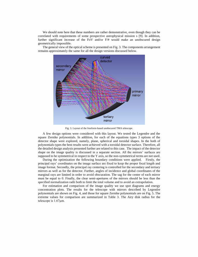
The general view of the optical scheme is presented on Fig. 3. The components arrangement
remains approximately the same for all the design versions discussed below.
Fig. 3. Layout of the freeform-based unobscured TMA telescope.
A few design options were considered with this layout. We tested the Legendre and the
square Zernike polynomials. In addition, for each of the equations types 3 options of the
detector shape were explored, namely, plane, spherical and toroidal shapes. In the both of
polynomials types the best results were achieved with a toroidal detector surface. Therefore, all
the detailed design analysis presented further are related to this case. The impact of the detector
shape on the image quality is discussed in a separate section. All the mirrors’ surfaces are
supposed to be symmetrical in respect to the Y axis, so the non-symmetrical terms are not used.
During the optimization the following boundary conditions were applied. Firstly, the
principal rays’ coordinates on the image surface are fixed to keep the proper focal length and
image format. Secondly, the principal ray centering is controlled for the secondary and tertiary
mirrors as well as for the detector. Further, angles of incidence and global coordinates of the
marginal rays are limited in order to avoid obscuration. The sag for the center of each mirror
must be equal to 0. Finally, the clear semi-apertures of the mirrors should be less than the
specified normalization radii both to limit the total volume and to avoid an extrapolation.
For estimation and comparison of the image quality we use spot diagrams and energy
concentration plots. The results for the telescope with mirrors described by Legendre
polynomials are shown on Fig. 4, and those for square Zernike polynomials are on Fig. 5. The
extreme values for comparison are summarized in Table 3. The Airy disk radius for the
telescope is 1.67µm.
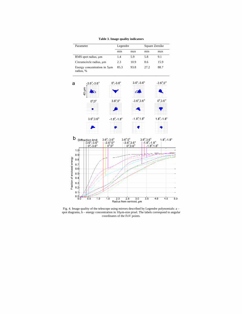
Table 3. Image quality indicators
Parameter Legendre Square Zernike
min max min max
RMS spot radius, µm 1.4 5.9 5.8 9.1
Circumcircle radius, µm 2.3 10.9 8.6 15.9
Energy concentration in 5µm radius, %
85.3 93.8 27.2 88.7
Fig. 4. Image quality of the telescope using mirrors described by Legendre polynomials: a – spot diagrams, b – energy concentration in 10µm-size pixel. The labels correspond to angular
coordinates of the FoV points.

Fig. 5. Image quality of the telescope using mirrors described by square Zernike polynomials:
a – spot diagrams, b – energy concentration in 10µm-size pixel. The labels correspond to
angular coordinates of the FoV points.
The diagrams clearly show that both of the polynomials types provides relatively good
aberration correction. However, the optical quality achieved with the Legendre polynomials is
obviously superior over that for the square Zernike polynomials. It approaches to the diffraction
limit for the central point and remains relatively uniform across all the wide 10°-diagonal field.
In addition to the image quality estimations shown above, it’s necessary to mention that the
design with Legendre polynomials has lower distortion (see Table 4). We can note that the
design with Legendre polynomials has some advantage. Also it should be noted that the
measured values are defined not only by a pure image distortion, but also by its’ residual shift,
which can be seen from the signs.
Table 4. Distortion of the telescopes in %
Measurement
direction
Legendre Square Zernike
X axis, positive -0.20 -0.19
X axis, negative -0.20 -0.19
Y axis, positive -0.25 -0.31
Y axis, negative -0.24 -0.15
Vectorial 1.33 1.38
Finally, both of the presented designs are notable for their compactness. Total volume of
the telescope with Legendre-type freeforms is approximately 233x416x507 mm, while that for
the design with square Zernike polynomials is 226x406x514 mm. Exact values will depend on
the mirrors thicknesses and mechanical design.
4. Analysis of the mirrors surfaces shapes
To assess complexity of the designed freeform surfaces we use difference between the
calculated surface sag and the best fit sphere (BFS). Here we define the BFS as a sphere with
variable radius and center position, which provides the smallest RMS error for the current
surface. It’s necessary to emphasize here that the BFS provides only an approximate estimation
for complexity and manufacturability of the freeforms, because in many cases [24] the surface
can be grinded directly into asphere, so a spherical blank is never actually used.
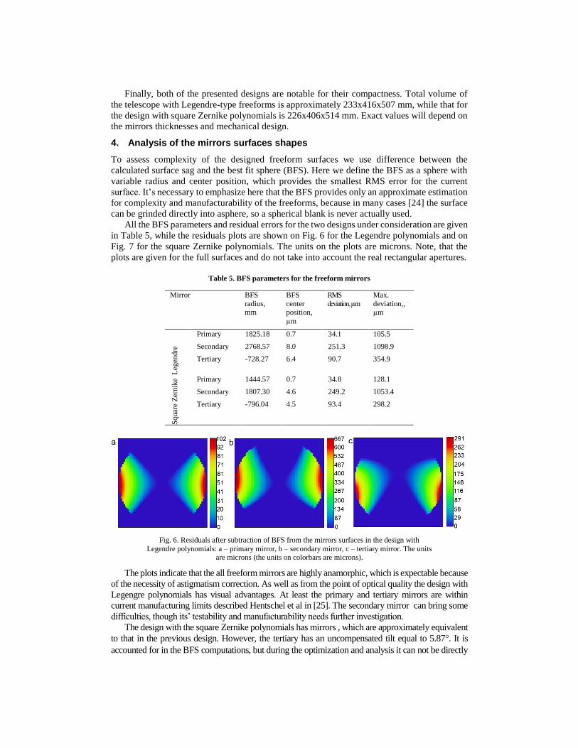
All the BFS parameters and residual errors for the two designs under consideration are given
in Table 5, while the residuals plots are shown on Fig. 6 for the Legendre polynomials and on
Fig. 7 for the square Zernike polynomials. The units on the plots are microns. Note, that the
plots are given for the full surfaces and do not take into account the real rectangular apertures.
Table 5. BFS parameters for the freeform mirrors
Mirror BFS
radius, mm
BFS
center position,
µm
RMS
deviation, µm
Max.
deviation,, µm
Leg
end
re
Primary 1825.18 0.7 34.1 105.5
Secondary 2768.57 8.0 251.3 1098.9
Tertiary -728.27 6.4 90.7 354.9
Sq
uar
e Z
ernik
e Primary 1444.57 0.7 34.8 128.1
Secondary 1807.30 4.6 249.2 1053.4
Tertiary -796.04 4.5 93.4
298.2
Fig. 6. Residuals after subtraction of BFS from the mirrors surfaces in the design with
Legendre polynomials: a – primary mirror, b – secondary mirror, c – tertiary mirror. The units are microns (the units on colorbars are microns).
The plots indicate that the all freeform mirrors are highly anamorphic, which is expectable because
of the necessity of astigmatism correction. As well as from the point of optical quality the design with
Legengre polynomials has visual advantages. At least the primary and tertiary mirrors are within
current manufacturing limits described Hentschel et al in [25]. The secondary mirror can bring some
difficulties, though its’ testability and manufacturability needs further investigation.
The design with the square Zernike polynomials has mirrors , which are approximately equivalent
to that in the previous design. However, the tertiary has an uncompensated tilt equal to 5.87°. It is
accounted for in the BFS computations, but during the optimization and analysis it can not be directly
removed, thus complicating the design process. This disadvantage is inherent to the square Zernike
polynomials and connected with the recurrent generating formulas.
Finally, it can be noted here that the tertiary mirror in both designs has the biggest optical
power. This feature is common for all the optical schemes considered during the study. That
propety can be useful for choice of an initial point for future designs.
Fig. 7. Residuals after subtraction of BFS from the mirrors surfaces in the design with square
Zernike polynomials: a – primary mirror, b – secondary mirror, c – tertiary mirror (the units on
colorbars are microns).
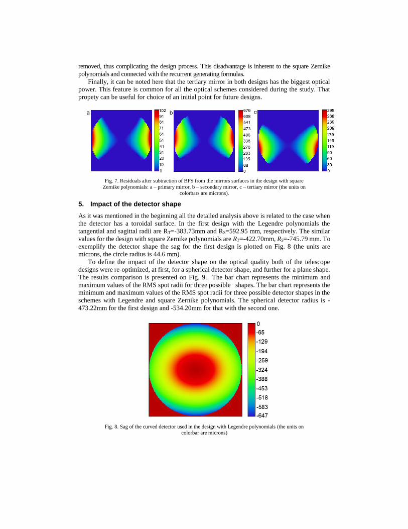
5. Impact of the detector shape
As it was mentioned in the beginning all the detailed analysis above is related to the case when
the detector has a toroidal surface. In the first design with the Legendre polynomials the
tangential and sagittal radii are RT=-383.73mm and RS=592.95 mm, respectively. The similar
values for the design with square Zernike polynomials are RT=-422.70mm, RS=-745.79 mm. To
exemplify the detector shape the sag for the first design is plotted on Fig. 8 (the units are
microns, the circle radius is 44.6 mm).
To define the impact of the detector shape on the optical quality both of the telescope
designs were re-optimized, at first, for a spherical detector shape, and further for a plane shape.
The results comparison is presented on Fig. 9. The bar chart represents the minimum and
maximum values of the RMS spot radii for three possible shapes. The bar chart represents the
minimum and maximum values of the RMS spot radii for three possible detector shapes in the
schemes with Legendre and square Zernike polynomials. The spherical detector radius is -
473.22mm for the first design and -534.20mm for that with the second one.
Fig. 8. Sag of the curved detector used in the design with Legendre polynomials (the units on colorbar are microns)
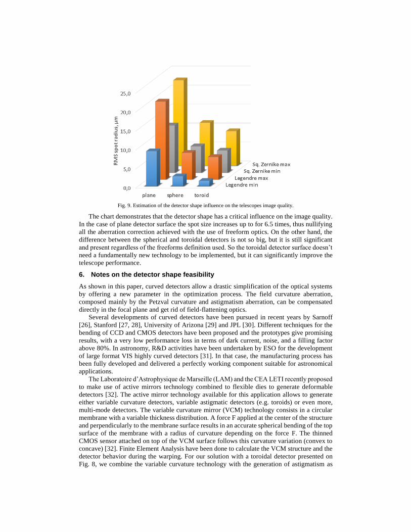
Fig. 9. Estimation of the detector shape influence on the telescopes image quality.
The chart demonstrates that the detector shape has a critical influence on the image quality.
In the case of plane detector surface the spot size increases up to for 6.5 times, thus nullifying
all the aberration correction achieved with the use of freeform optics. On the other hand, the
difference between the spherical and toroidal detectors is not so big, but it is still significant
and present regardless of the freeforms definition used. So the toroidal detector surface doesn’t
need a fundamentally new technology to be implemented, but it can significantly improve the
telescope performance.
6. Notes on the detector shape feasibility
As shown in this paper, curved detectors allow a drastic simplification of the optical systems
by offering a new parameter in the optimization process. The field curvature aberration,
composed mainly by the Petzval curvature and astigmatism aberration, can be compensated
directly in the focal plane and get rid of field-flattening optics.
Several developments of curved detectors have been pursued in recent years by Sarnoff
[26], Stanford [27, 28], University of Arizona [29] and JPL [30]. Different techniques for the
bending of CCD and CMOS detectors have been proposed and the prototypes give promising
results, with a very low performance loss in terms of dark current, noise, and a filling factor
above 80%. In astronomy, R&D activities have been undertaken by ESO for the development
of large format VIS highly curved detectors [31]. In that case, the manufacturing process has
been fully developed and delivered a perfectly working component suitable for astronomical
applications.
The Laboratoire d’Astrophysique de Marseille (LAM) and the CEA LETI recently proposed
to make use of active mirrors technology combined to flexible dies to generate deformable
detectors [32]. The active mirror technology available for this application allows to generate
either variable curvature detectors, variable astigmatic detectors (e.g. toroids) or even more,
multi-mode detectors. The variable curvature mirror (VCM) technology consists in a circular
membrane with a variable thickness distribution. A force F applied at the center of the structure
and perpendicularly to the membrane surface results in an accurate spherical bending of the top
surface of the membrane with a radius of curvature depending on the force F. The thinned
CMOS sensor attached on top of the VCM surface follows this curvature variation (convex to
concave) [32]. Finite Element Analysis have been done to calculate the VCM structure and the
detector behavior during the warping. For our solution with a toroidal detector presented on
Fig. 8, we combine the variable curvature technology with the generation of astigmatism as
presented in [34] to get the required toroidal shape. According to Figure 14 in [33], we are able
to curve a 30x30 mm size detector thinned at 100µm up to a radius of curvature of 140 mm. A
thickness of 100µm is the typical the value we use for our current developments. The toroidal
detector presents a tangential and sagittal radii of RT=-383.73mm and RS=592.95 mm, so 2.7
and 4.2 times more than the limitation value, making it safe to produce. Another way of bending
would be to use tunable active mirror technology [35] developed for space mission on which
the thinned CMOS sensor would be attached. This solution would allow to generate several
different shapes.
There are other recently presented versions of the curved sensors manufacturing
technology, for instance the pneumatic forming process described in [36].
7. Comparative study
The detailed description of the optical system given above should be complemented with a few
notes on its’ optimization process. Obviously, the obtained equations for the mirrors surfaces
shapes can be rewritten with different sets of polynomials. However, not all of them are equally
consistent with existing techniques and codes used for modelling and optimization of optical
systems. To exemplify the difference in optimization introduced by various polynomial sets we
provide we compare progress of optical quality achieved with Legendre, square Zernike,
standard Zernike and XY polynomials. In each case the starting point is an unobscured system
with three spherical mirrors and flat detector, which has F/# of 10 and FoV equal to 1.4°. Then
the surfaces are re-defined: the spheres are turned into freeforms with zero coefficients and the
detector plane is replaced by a toroidal with zero curvatures. The optical system passes through
a few steps of optimization with gradually growing values of aperture and FoV. The
optimization is performed by means of the standard damped least squares method [37], which
is implemented in Zemax. All the parameters defining shapes and positions of mirrors and
detector surfaces are used for optimization. The boundary conditions include only control of
the principal rays’ coordinates on the mirrors and the detector to maintain centering of the clear
apertures and proper focal length value, respectively. Boundaries for the components positions
are used to exclude obscuration and geometrical conflicts. There are also limits applied to the
mirrors diameters. Finally, the sag value for each mirror should equal to 0 in its’ center. The
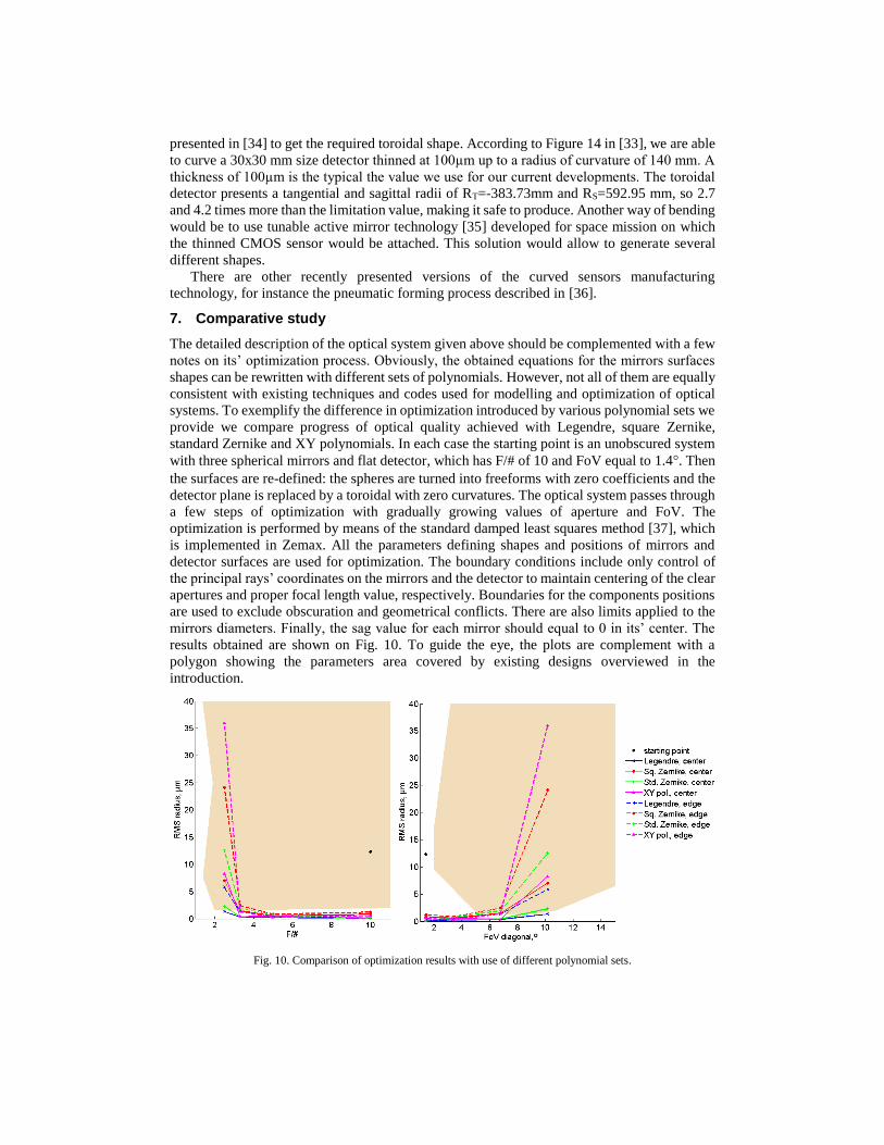
results obtained are shown on Fig. 10. To guide the eye, the plots are complement with a
polygon showing the parameters area covered by existing designs overviewed in the
introduction.
Fig. 10. Comparison of optimization results with use of different polynomial sets.
Thus, relying on the graphs we can conclude that with use of identical optimization
procedure Legendre polynomials allow to achieve better performance than other types of
equations. The non-normalized XY polynomials show the worst performance as it was
anticipated. The standard Zernike polynomials show notable decrease odf resolution for the
FoV edge. Possible explanation is the mismatch of clear apertures and circular basis, which is
hard to account for using standard optimization tools. Large spot radii values, obtained with the
square Zernike polynomials can represent a consequence of excessive complexity of the high-
order polynomials and the necessity to compensate for the intercept. Finally, it can be noted
that the image quality obtained for the FoV center with Legendre polynomials is slightly better
than for existing systems with the same F/# and FoV.
8. Conclusion
We considered possibility of use of two orthonormal sets of polynomials for design of freeform
mirrors, namely the Legendre polynomials and square Zernike polynomials. On an example of
unobscured all-reflective TMA-type telescope we demonstrated that application of such
polynomials for description of optical surfaces allows to achieve high performance for F/#
value up to 2.5 and over a large 10°-diagonal field of view.
The Legendre polynomials shows better results in terms of geometric aberrations and
energy concentration. The difference in the latter parameter for the field edge is as high as 3
times in comparison with the square Zernike polynomials. The mirrors surfaces designed with
the both of the polynomials sets are within the current manufacturability limits.
Finally, it was found that use of a toroidal shape of the detector surface can improve the
telescope performance significantly.
As our comparative study has demonstrated, use of the Legendre polynomials allows to
achieve very high performance in comparison with other types of equations, even if a very
simple starting point and only standard optimization tools are used.
In our opinion the use of the two considered sets of polynomials, especially the Legendre’s
ones, is a natural way to design freeform mirrors with square apertures. It can be easily
implemented in practice and matches with the standard optimization tools and techniques,
currently available for optical designers. We hope that the presented approach can become a
common one replacing use of ordinary XY-polynomials and suggesting an alternative to the
standard Zernike polynomials.
The developed telescope design represents a self-sufficient result, which can be of a special
interest for some applications like that described in [9]. Further it can be considered in more
details including the questions of tolerancing, mirrors manufacturing and testing, opto-
mechanical design and assembling of the telescope.
Funding.
ERC(European Research Council) (H2020-ERC-STG-2015 – 678777).
Acknowledgment.
The authors acknowledge the support of the European Research council through the H2020 -
ERC-STG-2015 – 678777 ICARUS program.