Embed Size (px)
Citation preview
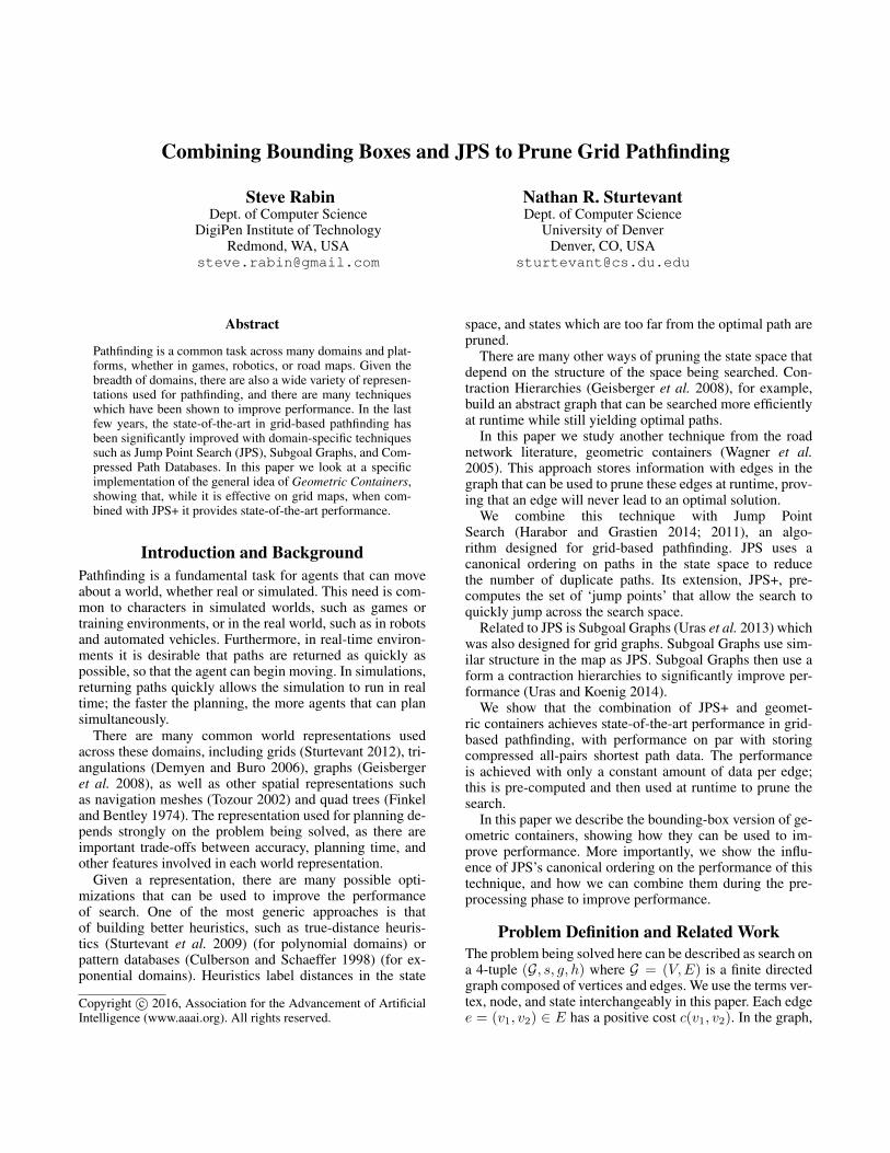
Combining Bounding Boxes and JPS to Prune Grid Pathfinding
Steve RabinDept. of Computer Science
DigiPen Institute of TechnologyRedmond, WA, USA
Nathan R. SturtevantDept. of Computer Science
University of DenverDenver, CO, USA
Abstract
Pathfinding is a common task across many domains and plat-forms, whether in games, robotics, or road maps. Given thebreadth of domains, there are also a wide variety of represen-tations used for pathfinding, and there are many techniqueswhich have been shown to improve performance. In the lastfew years, the state-of-the-art in grid-based pathfinding hasbeen significantly improved with domain-specific techniquessuch as Jump Point Search (JPS), Subgoal Graphs, and Com-pressed Path Databases. In this paper we look at a specificimplementation of the general idea of Geometric Containers,showing that, while it is effective on grid maps, when com-bined with JPS+ it provides state-of-the-art performance.
Introduction and BackgroundPathfinding is a fundamental task for agents that can moveabout a world, whether real or simulated. This need is com-mon to characters in simulated worlds, such as games ortraining environments, or in the real world, such as in robotsand automated vehicles. Furthermore, in real-time environ-ments it is desirable that paths are returned as quickly aspossible, so that the agent can begin moving. In simulations,returning paths quickly allows the simulation to run in realtime; the faster the planning, the more agents that can plansimultaneously.
There are many common world representations usedacross these domains, including grids (Sturtevant 2012), tri-angulations (Demyen and Buro 2006), graphs (Geisbergeret al. 2008), as well as other spatial representations suchas navigation meshes (Tozour 2002) and quad trees (Finkeland Bentley 1974). The representation used for planning de-pends strongly on the problem being solved, as there areimportant trade-offs between accuracy, planning time, andother features involved in each world representation.
Given a representation, there are many possible opti-mizations that can be used to improve the performanceof search. One of the most generic approaches is thatof building better heuristics, such as true-distance heuris-tics (Sturtevant et al. 2009) (for polynomial domains) orpattern databases (Culberson and Schaeffer 1998) (for ex-ponential domains). Heuristics label distances in the state
Copyright c© 2016, Association for the Advancement of ArtificialIntelligence (www.aaai.org). All rights reserved.
space, and states which are too far from the optimal path arepruned.
There are many other ways of pruning the state space thatdepend on the structure of the space being searched. Con-traction Hierarchies (Geisberger et al. 2008), for example,build an abstract graph that can be searched more efficientlyat runtime while still yielding optimal paths.
In this paper we study another technique from the roadnetwork literature, geometric containers (Wagner et al.2005). This approach stores information with edges in thegraph that can be used to prune these edges at runtime, prov-ing that an edge will never lead to an optimal solution.
We combine this technique with Jump PointSearch (Harabor and Grastien 2014; 2011), an algo-rithm designed for grid-based pathfinding. JPS uses acanonical ordering on paths in the state space to reducethe number of duplicate paths. Its extension, JPS+, pre-computes the set of ‘jump points’ that allow the search toquickly jump across the search space.
Related to JPS is Subgoal Graphs (Uras et al. 2013) whichwas also designed for grid graphs. Subgoal Graphs use sim-ilar structure in the map as JPS. Subgoal Graphs then use aform a contraction hierarchies to significantly improve per-formance (Uras and Koenig 2014).
We show that the combination of JPS+ and geomet-ric containers achieves state-of-the-art performance in grid-based pathfinding, with performance on par with storingcompressed all-pairs shortest path data. The performanceis achieved with only a constant amount of data per edge;this is pre-computed and then used at runtime to prune thesearch.
In this paper we describe the bounding-box version of ge-ometric containers, showing how they can be used to im-prove performance. More importantly, we show the influ-ence of JPS’s canonical ordering on the performance of thistechnique, and how we can combine them during the pre-processing phase to improve performance.
Problem Definition and Related WorkThe problem being solved here can be described as search ona 4-tuple (G, s, g, h) where G = (V,E) is a finite directedgraph composed of vertices and edges. We use the terms ver-tex, node, and state interchangeably in this paper. Each edgee = (v1, v2) ∈ E has a positive cost c(v1, v2). In the graph,
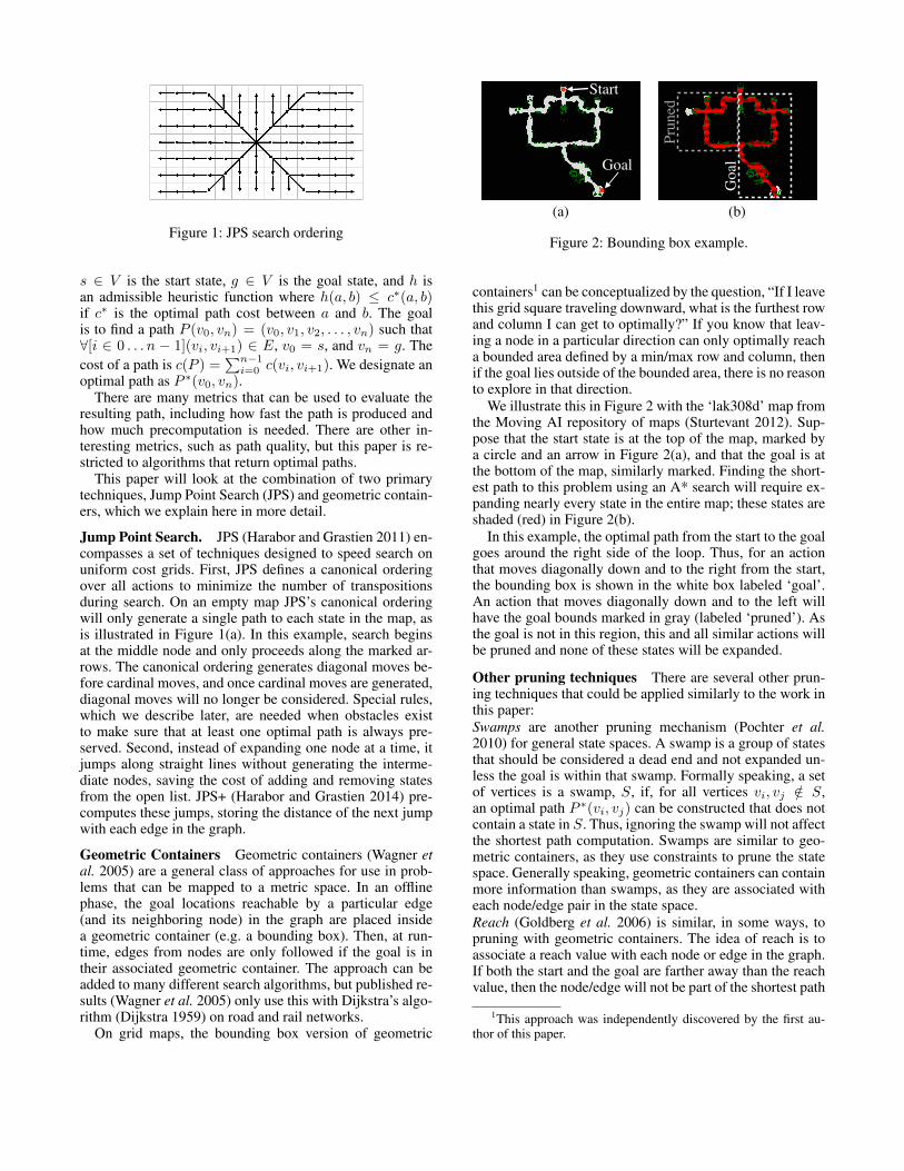
Figure 1: JPS search ordering
s ∈ V is the start state, g ∈ V is the goal state, and h isan admissible heuristic function where h(a, b) ≤ c∗(a, b)if c∗ is the optimal path cost between a and b. The goalis to find a path P (v0, vn) = (v0, v1, v2, . . . , vn) such that∀[i ∈ 0 . . . n − 1](vi, vi+1) ∈ E, v0 = s, and vn = g. Thecost of a path is c(P ) =
∑n−1i=0 c(vi, vi+1). We designate an
optimal path as P ∗(v0, vn).There are many metrics that can be used to evaluate the
resulting path, including how fast the path is produced andhow much precomputation is needed. There are other in-teresting metrics, such as path quality, but this paper is re-stricted to algorithms that return optimal paths.
This paper will look at the combination of two primarytechniques, Jump Point Search (JPS) and geometric contain-ers, which we explain here in more detail.
Jump Point Search. JPS (Harabor and Grastien 2011) en-compasses a set of techniques designed to speed search onuniform cost grids. First, JPS defines a canonical orderingover all actions to minimize the number of transpositionsduring search. On an empty map JPS’s canonical orderingwill only generate a single path to each state in the map, asis illustrated in Figure 1(a). In this example, search beginsat the middle node and only proceeds along the marked ar-rows. The canonical ordering generates diagonal moves be-fore cardinal moves, and once cardinal moves are generated,diagonal moves will no longer be considered. Special rules,which we describe later, are needed when obstacles existto make sure that at least one optimal path is always pre-served. Second, instead of expanding one node at a time, itjumps along straight lines without generating the interme-diate nodes, saving the cost of adding and removing statesfrom the open list. JPS+ (Harabor and Grastien 2014) pre-computes these jumps, storing the distance of the next jumpwith each edge in the graph.
Geometric Containers Geometric containers (Wagner etal. 2005) are a general class of approaches for use in prob-lems that can be mapped to a metric space. In an offlinephase, the goal locations reachable by a particular edge(and its neighboring node) in the graph are placed insidea geometric container (e.g. a bounding box). Then, at run-time, edges from nodes are only followed if the goal is intheir associated geometric container. The approach can beadded to many different search algorithms, but published re-sults (Wagner et al. 2005) only use this with Dijkstra’s algo-rithm (Dijkstra 1959) on road and rail networks.
On grid maps, the bounding box version of geometric
Start
Goal
•
•
Pruned
Goal
(a) (b)
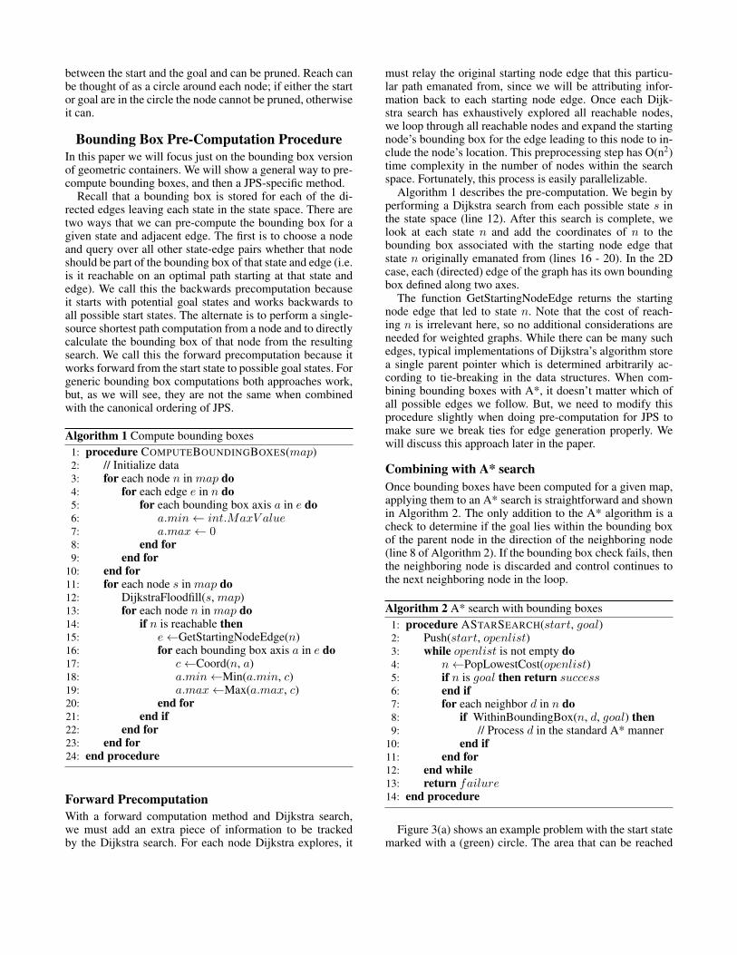
Figure 2: Bounding box example.
containers1 can be conceptualized by the question, “If I leavethis grid square traveling downward, what is the furthest rowand column I can get to optimally?” If you know that leav-ing a node in a particular direction can only optimally reacha bounded area defined by a min/max row and column, thenif the goal lies outside of the bounded area, there is no reasonto explore in that direction.
We illustrate this in Figure 2 with the ‘lak308d’ map fromthe Moving AI repository of maps (Sturtevant 2012). Sup-pose that the start state is at the top of the map, marked bya circle and an arrow in Figure 2(a), and that the goal is atthe bottom of the map, similarly marked. Finding the short-est path to this problem using an A* search will require ex-panding nearly every state in the entire map; these states areshaded (red) in Figure 2(b).
In this example, the optimal path from the start to the goalgoes around the right side of the loop. Thus, for an actionthat moves diagonally down and to the right from the start,the bounding box is shown in the white box labeled ‘goal’.An action that moves diagonally down and to the left willhave the goal bounds marked in gray (labeled ‘pruned’). Asthe goal is not in this region, this and all similar actions willbe pruned and none of these states will be expanded.
Other pruning techniques There are several other prun-ing techniques that could be applied similarly to the work inthis paper:Swamps are another pruning mechanism (Pochter et al.2010) for general state spaces. A swamp is a group of statesthat should be considered a dead end and not expanded un-less the goal is within that swamp. Formally speaking, a setof vertices is a swamp, S, if, for all vertices vi, vj /∈ S,an optimal path P ∗(vi, vj) can be constructed that does notcontain a state in S. Thus, ignoring the swamp will not affectthe shortest path computation. Swamps are similar to geo-metric containers, as they use constraints to prune the statespace. Generally speaking, geometric containers can containmore information than swamps, as they are associated witheach node/edge pair in the state space.Reach (Goldberg et al. 2006) is similar, in some ways, topruning with geometric containers. The idea of reach is toassociate a reach value with each node or edge in the graph.If both the start and the goal are farther away than the reachvalue, then the node/edge will not be part of the shortest path
1This approach was independently discovered by the first au-thor of this paper.
between the start and the goal and can be pruned. Reach canbe thought of as a circle around each node; if either the startor goal are in the circle the node cannot be pruned, otherwiseit can.
Bounding Box Pre-Computation ProcedureIn this paper we will focus just on the bounding box versionof geometric containers. We will show a general way to pre-compute bounding boxes, and then a JPS-specific method.
Recall that a bounding box is stored for each of the di-rected edges leaving each state in the state space. There aretwo ways that we can pre-compute the bounding box for agiven state and adjacent edge. The first is to choose a nodeand query over all other state-edge pairs whether that nodeshould be part of the bounding box of that state and edge (i.e.is it reachable on an optimal path starting at that state andedge). We call this the backwards precomputation becauseit starts with potential goal states and works backwards toall possible start states. The alternate is to perform a single-source shortest path computation from a node and to directlycalculate the bounding box of that node from the resultingsearch. We call this the forward precomputation because itworks forward from the start state to possible goal states. Forgeneric bounding box computations both approaches work,but, as we will see, they are not the same when combinedwith the canonical ordering of JPS.
Algorithm 1 Compute bounding boxes1: procedure COMPUTEBOUNDINGBOXES(map)2: // Initialize data3: for each node n in map do4: for each edge e in n do5: for each bounding box axis a in e do6: a.min← int.MaxV alue7: a.max← 08: end for9: end for
10: end for11: for each node s in map do12: DijkstraFloodfill(s, map)13: for each node n in map do14: if n is reachable then15: e←GetStartingNodeEdge(n)16: for each bounding box axis a in e do17: c←Coord(n, a)18: a.min←Min(a.min, c)19: a.max←Max(a.max, c)20: end for21: end if22: end for23: end for24: end procedure
Forward PrecomputationWith a forward computation method and Dijkstra search,we must add an extra piece of information to be trackedby the Dijkstra search. For each node Dijkstra explores, it
must relay the original starting node edge that this particu-lar path emanated from, since we will be attributing infor-mation back to each starting node edge. Once each Dijk-stra search has exhaustively explored all reachable nodes,we loop through all reachable nodes and expand the startingnode’s bounding box for the edge leading to this node to in-clude the node’s location. This preprocessing step has O(n2)time complexity in the number of nodes within the searchspace. Fortunately, this process is easily parallelizable.
Algorithm 1 describes the pre-computation. We begin byperforming a Dijkstra search from each possible state s inthe state space (line 12). After this search is complete, welook at each state n and add the coordinates of n to thebounding box associated with the starting node edge thatstate n originally emanated from (lines 16 - 20). In the 2Dcase, each (directed) edge of the graph has its own boundingbox defined along two axes.
The function GetStartingNodeEdge returns the startingnode edge that led to state n. Note that the cost of reach-ing n is irrelevant here, so no additional considerations areneeded for weighted graphs. While there can be many suchedges, typical implementations of Dijkstra’s algorithm storea single parent pointer which is determined arbitrarily ac-cording to tie-breaking in the data structures. When com-bining bounding boxes with A*, it doesn’t matter which ofall possible edges we follow. But, we need to modify thisprocedure slightly when doing pre-computation for JPS tomake sure we break ties for edge generation properly. Wewill discuss this approach later in the paper.
Combining with A* searchOnce bounding boxes have been computed for a given map,applying them to an A* search is straightforward and shownin Algorithm 2. The only addition to the A* algorithm is acheck to determine if the goal lies within the bounding boxof the parent node in the direction of the neighboring node(line 8 of Algorithm 2). If the bounding box check fails, thenthe neighboring node is discarded and control continues tothe next neighboring node in the loop.
Algorithm 2 A* search with bounding boxes1: procedure ASTARSEARCH(start, goal)2: Push(start, openlist)3: while openlist is not empty do4: n←PopLowestCost(openlist)5: if n is goal then return success6: end if7: for each neighbor d in n do8: if WithinBoundingBox(n, d, goal) then9: // Process d in the standard A* manner
10: end if11: end for12: end while13: return failure14: end procedure
Figure 3(a) shows an example problem with the start statemarked with a (green) circle. The area that can be reached
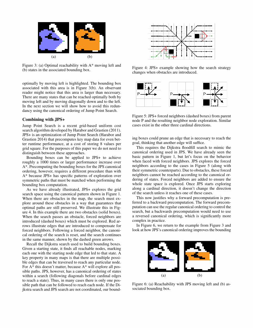
(a) (b)
Figure 3: (a) Optimal reachability with A* moving left and(b) states in the associated bounding box.
optimally by moving left is highlighted. The bounding boxassociated with this area is in Figure 3(b). An observantreader might notice that this area is larger than necessary.There are many states that can be reached optimally both bymoving left and by moving diagonally down and to the left.In the next section we will show how to avoid this redun-dancy using the canonical ordering of Jump Point Search.
Combining with JPS+Jump Point Search is a recent grid-based uniform costsearch algorithm developed by Harabor and Grastien (2011).JPS+ is an optimization of Jump Point Search (Harabor andGrastien 2014) that precomputes key map data for even bet-ter runtime performance, at a cost of storing 8 values pergrid square. For the purposes of this paper we do not need todistinguish between these approaches.
Bounding boxes can be applied to JPS+ to achieveroughly a 1000 times or larger performance increase overA*. Precomputing the bounding boxes for the JPS canonicalordering, however, requires a different procedure than withA* because JPS+ has specific patterns of exploration oversymmetric paths that must be matched when performing thebounding box computation.
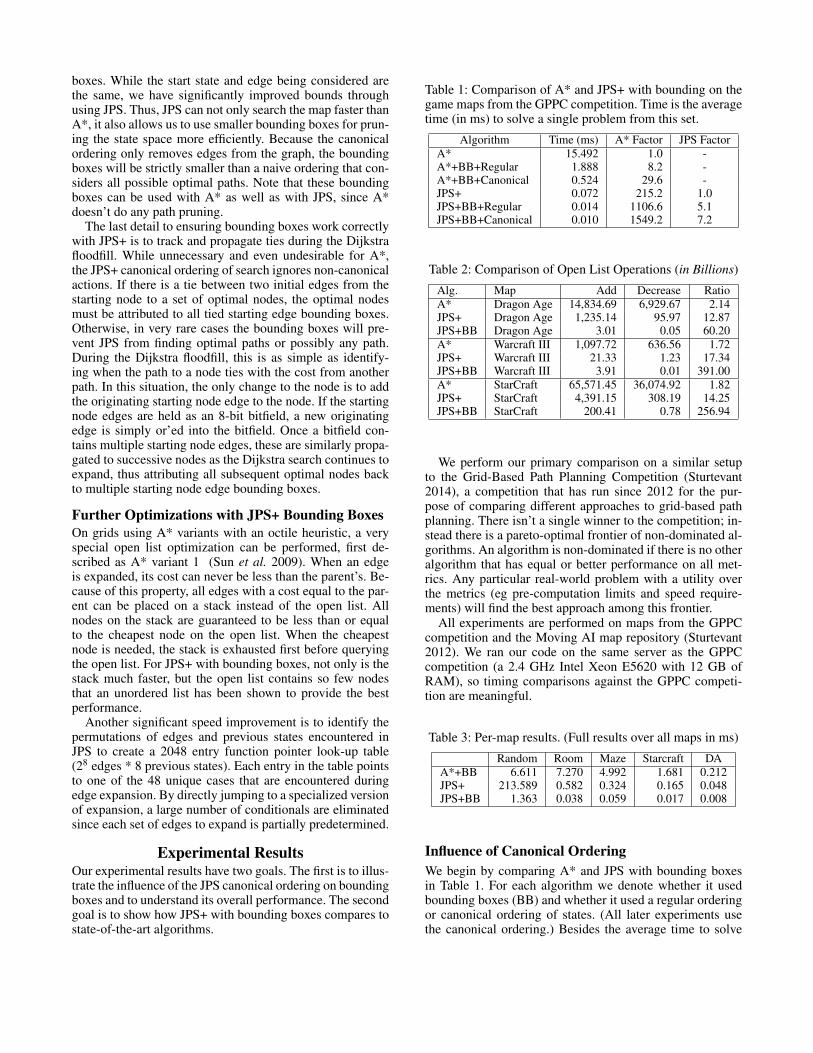
As we have already illustrated, JPS+ explores the gridsearch space using the canonical pattern shown in Figure 1.When there are obstacles in the map, the search must ex-plore around these obstacles in a way that guarantees thatoptimal paths are still preserved. We illustrate this in Fig-ure 4. In this example there are two obstacles (solid boxes).When the search passes an obstacle, forced neighbors areintroduced (dashed boxes) which must be explored. Red ar-rows illustrate edges that are introduced to compensate forforced neighbors. Following a forced neighbor, the canoni-cal ordering of the search is reset, and the search continuesin the same manner, shown by the dashed green arrows.
Recall the Dijkstra search used to build bounding boxes.Given a starting state, it finds all reachable nodes, markingeach one with the starting node edge that led to that state. Akey property in many maps is that there are multiple possi-ble edges that can be traversed to reach any particular node.For A* this doesn’t matter, because A* will explore all pos-sible paths. JPS, however, has a canonical ordering of stateswithin a search (following diagonals before cardinal edgesto reach a state). Thus, in many cases there is only one pos-sible path that can be followed to reach each node. If the Di-jkstra search and JPS search are not coordinated, our bound-
Figure 4: JPS+ example showing how the search strategychanges when obstacles are introduced.
Figure 5: JPS+ forced neighbors (dashed boxes) from parentnode P and the resulting neighbor node exploration. Similarcases exist in the other three cardinal directions.
ing boxes could prune an edge that is necessary to reach thegoal, thinking that another edge will suffice.
This requires the Dijkstra floodfill search to mimic thecanonical ordering used in JPS. We have already seen thebasic pattern in Figure 1, but let’s focus on the behaviorwhen faced with forced neighbors. JPS explores the forcedneighbors according to the cases in Figure 5 (along withtheir symmetric counterparts). Due to obstacles, these forcedneighbors cannot be reached according to the canonical or-dering of states. Forced neighbors are added to ensure thewhole state space is explored. Once JPS starts exploringalong a cardinal direction, it doesn’t change the directionof the search unless it reaches one of these cases.
This now justifies why a forward precomputation is pre-ferred to a backward precomputation. The forward precom-putation can use the regular canonical ordering to control thesearch, but a backwards precomputation would need to usea reversed canonical ordering, which is significantly morecomplex in practice.
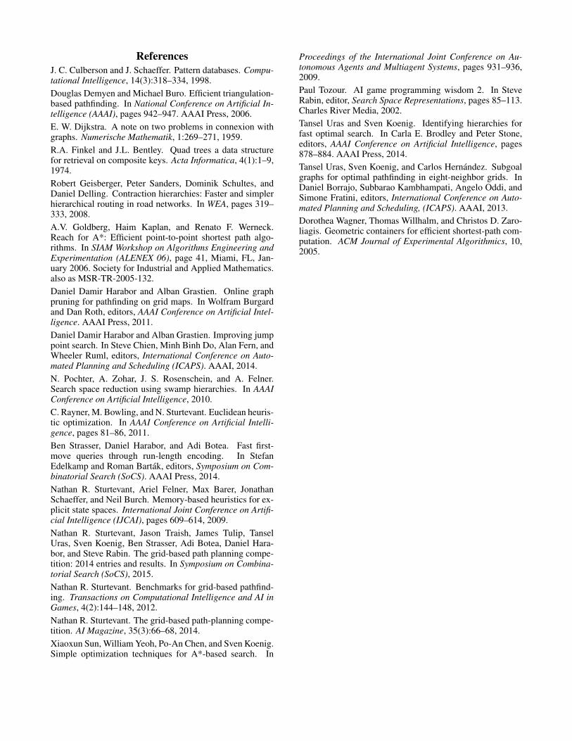
In Figure 6, we return to the example from Figure 3 andlook at how JPS’s canonical ordering improves the bounding
(a) (b)
Figure 6: (a) Reachability with JPS moving left and (b) as-sociated bounding box.
boxes. While the start state and edge being considered arethe same, we have significantly improved bounds throughusing JPS. Thus, JPS can not only search the map faster thanA*, it also allows us to use smaller bounding boxes for prun-ing the state space more efficiently. Because the canonicalordering only removes edges from the graph, the boundingboxes will be strictly smaller than a naive ordering that con-siders all possible optimal paths. Note that these boundingboxes can be used with A* as well as with JPS, since A*doesn’t do any path pruning.
The last detail to ensuring bounding boxes work correctlywith JPS+ is to track and propagate ties during the Dijkstrafloodfill. While unnecessary and even undesirable for A*,the JPS+ canonical ordering of search ignores non-canonicalactions. If there is a tie between two initial edges from thestarting node to a set of optimal nodes, the optimal nodesmust be attributed to all tied starting edge bounding boxes.Otherwise, in very rare cases the bounding boxes will pre-vent JPS from finding optimal paths or possibly any path.During the Dijkstra floodfill, this is as simple as identify-ing when the path to a node ties with the cost from anotherpath. In this situation, the only change to the node is to addthe originating starting node edge to the node. If the startingnode edges are held as an 8-bit bitfield, a new originatingedge is simply or’ed into the bitfield. Once a bitfield con-tains multiple starting node edges, these are similarly propa-gated to successive nodes as the Dijkstra search continues toexpand, thus attributing all subsequent optimal nodes backto multiple starting node edge bounding boxes.
Further Optimizations with JPS+ Bounding BoxesOn grids using A* variants with an octile heuristic, a veryspecial open list optimization can be performed, first de-scribed as A* variant 1 (Sun et al. 2009). When an edgeis expanded, its cost can never be less than the parent’s. Be-cause of this property, all edges with a cost equal to the par-ent can be placed on a stack instead of the open list. Allnodes on the stack are guaranteed to be less than or equalto the cheapest node on the open list. When the cheapestnode is needed, the stack is exhausted first before queryingthe open list. For JPS+ with bounding boxes, not only is thestack much faster, but the open list contains so few nodesthat an unordered list has been shown to provide the bestperformance.
Another significant speed improvement is to identify thepermutations of edges and previous states encountered inJPS to create a 2048 entry function pointer look-up table(28 edges * 8 previous states). Each entry in the table pointsto one of the 48 unique cases that are encountered duringedge expansion. By directly jumping to a specialized versionof expansion, a large number of conditionals are eliminatedsince each set of edges to expand is partially predetermined.
Experimental ResultsOur experimental results have two goals. The first is to illus-trate the influence of the JPS canonical ordering on boundingboxes and to understand its overall performance. The secondgoal is to show how JPS+ with bounding boxes compares tostate-of-the-art algorithms.
Table 1: Comparison of A* and JPS+ with bounding on thegame maps from the GPPC competition. Time is the averagetime (in ms) to solve a single problem from this set.
Algorithm Time (ms) A* Factor JPS FactorA* 15.492 1.0 -A*+BB+Regular 1.888 8.2 -A*+BB+Canonical 0.524 29.6 -JPS+ 0.072 215.2 1.0JPS+BB+Regular 0.014 1106.6 5.1JPS+BB+Canonical 0.010 1549.2 7.2
Table 2: Comparison of Open List Operations (in Billions)
Alg. Map Add Decrease RatioA* Dragon Age 14,834.69 6,929.67 2.14JPS+ Dragon Age 1,235.14 95.97 12.87JPS+BB Dragon Age 3.01 0.05 60.20A* Warcraft III 1,097.72 636.56 1.72JPS+ Warcraft III 21.33 1.23 17.34JPS+BB Warcraft III 3.91 0.01 391.00A* StarCraft 65,571.45 36,074.92 1.82JPS+ StarCraft 4,391.15 308.19 14.25JPS+BB StarCraft 200.41 0.78 256.94
We perform our primary comparison on a similar setupto the Grid-Based Path Planning Competition (Sturtevant2014), a competition that has run since 2012 for the pur-pose of comparing different approaches to grid-based pathplanning. There isn’t a single winner to the competition; in-stead there is a pareto-optimal frontier of non-dominated al-gorithms. An algorithm is non-dominated if there is no otheralgorithm that has equal or better performance on all met-rics. Any particular real-world problem with a utility overthe metrics (eg pre-computation limits and speed require-ments) will find the best approach among this frontier.
All experiments are performed on maps from the GPPCcompetition and the Moving AI map repository (Sturtevant2012). We ran our code on the same server as the GPPCcompetition (a 2.4 GHz Intel Xeon E5620 with 12 GB ofRAM), so timing comparisons against the GPPC competi-tion are meaningful.
Table 3: Per-map results. (Full results over all maps in ms)
Random Room Maze Starcraft DAA*+BB 6.611 7.270 4.992 1.681 0.212JPS+ 213.589 0.582 0.324 0.165 0.048JPS+BB 1.363 0.038 0.059 0.017 0.008
Influence of Canonical OrderingWe begin by comparing A* and JPS with bounding boxesin Table 1. For each algorithm we denote whether it usedbounding boxes (BB) and whether it used a regular orderingor canonical ordering of states. (All later experiments usethe canonical ordering.) Besides the average time to solve
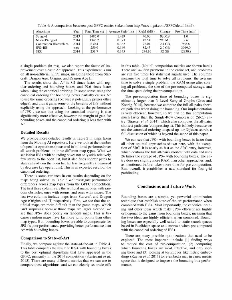
Table 4: A comparison between past GPPC entries (taken from http://movingai.com/GPPC/detail.html).
Algorithm Year Total Time (s) Average Path (ms) RAM (MB) Storage Pre-Time (min)Subgoal 2013 2485.0 1.429 40.00 93 MB 1.0NLevelSubgoal 2014 1345.2 0.773 42.54 293 MB 2.6Contraction Hierarchies 2014 630.4 0.362 72.04 2.4 GB 968.8JPS+BB new 259.9 0.149 82.43 2.0 GB 3049.0SRC 2014 251.7 0.145 274.16 52 GB 12330.8
a single problem (in ms), we also report the factor of im-provement over a basic A* approach. This experiment is runon all non-artificial GPPC maps, including those from Star-craft, Dragon Age: Origins, and Dragon Age II.
The results show that A* is 8.2 times faster with reg-ular ordering and bounding boxes, and 29.6 times fasterwhen using the canonical ordering. In some sense, using thecanonical ordering for bounding boxes partially causes A*to use the same ordering (because it potentially prunes otheredges), and thus it gains some of the benefits of JPS withoutexplicitly using the approach. Looking at the performanceof JPS+, we see that using the canonical ordering is alsosignificantly more effective, however the margin of gain forbounding boxes and the canonical ordering is less than withA*.
Detailed ResultsWe provide more detailed results in Table 2 in maps takenfrom the Moving AI repository. Here we look at the numberof open list operations (measured in billions) performed overall search problems on three different map types. What wesee is that JPS+ with bounding boxes not only adds relativelyfew states to the open list, but it also finds shorter paths tostates already on the open list far less frequently (measuredby decrease key operations). This is an expected result of thecanonical ordering.
There is some variance in our results depending on themaps being solved. In Table 3 we investigate performancedifferences across map types from the GPPC competition.The first three columns are the artificial maps: ones with ran-dom obstacles, ones with rooms, and ones with mazes. Thelast two columns include maps from Starcraft and DragonAge (Origins and II) respectively. First, we see that the ar-tificial maps are more difficult than the game maps, whichisn’t surprising because those maps are larger. Second, wesee that JPS+ does poorly on random maps. This is be-cause random maps have far more jump points than othermap types. But, bounding boxes are able to compensate forJPS+’s poor performance, providing better performance thanA* with bounding boxes.
Comparison to State-of-ArtFinally, we compare against the state-of-the-art in Table 4.This table compares the result of JPS+ with bounding boxesto the best optimal algorithms that have appeared in theGPPC, primarily in the 2014 competition (Sturtevant et al.2015). There are many different metrics that we can use tocompare these algorithms, and we can clearly see trade-offs
in this table. (Not all competition metrics are shown here.)There are 347,868 problems in the entire set, and problemsare run five times for statistical significance. The columnsmeasure the total time to solve all problems, the averagetime to solve a single problem, the RAM usage after solv-ing all problems, the size of the pre-computed storage, andthe time spent doing the precomputation.
The pre-computation time of bounding boxes is sig-nificantly larger than N-Level Subgoal Graphs (Uras andKoenig 2014), because we compute the full all-pairs short-est path data when doing the bounding. Our implementationis very efficient, however, so we can do this computationmuch faster than the Single-Row Compression (SRC) en-try (Strasser et al. 2014), which also computes the all-pairsshortest-path data (compressing it). This is likely because weuse the canonical ordering to speed up our Dijkstra search, afull discussion of which is beyond the scope of this paper.
We can see that JPS+ with bounding boxes is faster thanall other optimal approaches shown here, with the excep-tion of SRC. It is nearly as fast as the SRC entry, however,which contains the full all-pairs shortest path data and uses26 times the storage of JPS+ with bounding boxes. The en-try does use slightly more RAM than other approaches, and,as mentioned before, takes more time for pre-computation.But, overall, it establishes a new standard for fast gridpathfinding.
Conclusions and Future Work
Bounding boxes are a simple, yet powerful optimizationtechnique that establish state-of-the-art performance whencombined with JPS+. Most importantly, the canonical prun-ing and other ideas which make JPS+ efficient are highlyorthogonal to the gains from bounding boxes, meaning thatthe two ideas are highly efficient when combined. Bound-ing boxes are especially well suited to static search spacesbased in Euclidean space and improve when pre-computedwith the canonical ordering of JPS+.
There are many possible optimizations that need to beexplored. The most important include (1) finding waysto reduce the cost of pre-computation, (2) computingwhich bounding boxes are most effective, and only stor-ing these and (3) looking at techniques like metric embed-dings (Rayner et al. 2011) to re-embed a map in a new metricspace that is designed to improve the bounding box perfor-mance.
ReferencesJ. C. Culberson and J. Schaeffer. Pattern databases. Compu-tational Intelligence, 14(3):318–334, 1998.Douglas Demyen and Michael Buro. Efficient triangulation-based pathfinding. In National Conference on Artificial In-telligence (AAAI), pages 942–947. AAAI Press, 2006.E. W. Dijkstra. A note on two problems in connexion withgraphs. Numerische Mathematik, 1:269–271, 1959.R.A. Finkel and J.L. Bentley. Quad trees a data structurefor retrieval on composite keys. Acta Informatica, 4(1):1–9,1974.Robert Geisberger, Peter Sanders, Dominik Schultes, andDaniel Delling. Contraction hierarchies: Faster and simplerhierarchical routing in road networks. In WEA, pages 319–333, 2008.A.V. Goldberg, Haim Kaplan, and Renato F. Werneck.Reach for A*: Efficient point-to-point shortest path algo-rithms. In SIAM Workshop on Algorithms Engineering andExperimentation (ALENEX 06), page 41, Miami, FL, Jan-uary 2006. Society for Industrial and Applied Mathematics.also as MSR-TR-2005-132.Daniel Damir Harabor and Alban Grastien. Online graphpruning for pathfinding on grid maps. In Wolfram Burgardand Dan Roth, editors, AAAI Conference on Artificial Intel-ligence. AAAI Press, 2011.Daniel Damir Harabor and Alban Grastien. Improving jumppoint search. In Steve Chien, Minh Binh Do, Alan Fern, andWheeler Ruml, editors, International Conference on Auto-mated Planning and Scheduling (ICAPS). AAAI, 2014.N. Pochter, A. Zohar, J. S. Rosenschein, and A. Felner.Search space reduction using swamp hierarchies. In AAAIConference on Artificial Intelligence, 2010.C. Rayner, M. Bowling, and N. Sturtevant. Euclidean heuris-tic optimization. In AAAI Conference on Artificial Intelli-gence, pages 81–86, 2011.Ben Strasser, Daniel Harabor, and Adi Botea. Fast first-move queries through run-length encoding. In StefanEdelkamp and Roman Bartak, editors, Symposium on Com-binatorial Search (SoCS). AAAI Press, 2014.Nathan R. Sturtevant, Ariel Felner, Max Barer, JonathanSchaeffer, and Neil Burch. Memory-based heuristics for ex-plicit state spaces. International Joint Conference on Artifi-cial Intelligence (IJCAI), pages 609–614, 2009.Nathan R. Sturtevant, Jason Traish, James Tulip, TanselUras, Sven Koenig, Ben Strasser, Adi Botea, Daniel Hara-bor, and Steve Rabin. The grid-based path planning compe-tition: 2014 entries and results. In Symposium on Combina-torial Search (SoCS), 2015.Nathan R. Sturtevant. Benchmarks for grid-based pathfind-ing. Transactions on Computational Intelligence and AI inGames, 4(2):144–148, 2012.Nathan R. Sturtevant. The grid-based path-planning compe-tition. AI Magazine, 35(3):66–68, 2014.Xiaoxun Sun, William Yeoh, Po-An Chen, and Sven Koenig.Simple optimization techniques for A*-based search. In
Proceedings of the International Joint Conference on Au-tonomous Agents and Multiagent Systems, pages 931–936,2009.Paul Tozour. AI game programming wisdom 2. In SteveRabin, editor, Search Space Representations, pages 85–113.Charles River Media, 2002.Tansel Uras and Sven Koenig. Identifying hierarchies forfast optimal search. In Carla E. Brodley and Peter Stone,editors, AAAI Conference on Artificial Intelligence, pages878–884. AAAI Press, 2014.Tansel Uras, Sven Koenig, and Carlos Hernandez. Subgoalgraphs for optimal pathfinding in eight-neighbor grids. InDaniel Borrajo, Subbarao Kambhampati, Angelo Oddi, andSimone Fratini, editors, International Conference on Auto-mated Planning and Scheduling, (ICAPS). AAAI, 2013.Dorothea Wagner, Thomas Willhalm, and Christos D. Zaro-liagis. Geometric containers for efficient shortest-path com-putation. ACM Journal of Experimental Algorithmics, 10,2005.