Embed Size (px)
Citation preview
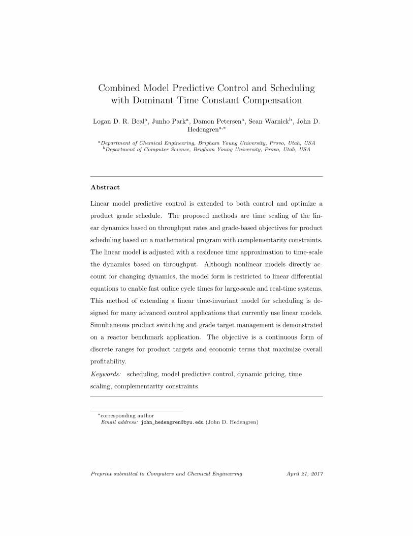
Combined Model Predictive Control and Schedulingwith Dominant Time Constant Compensation
Logan D. R. Beala, Junho Parka, Damon Petersena, Sean Warnickb, John D.Hedengrena,∗
aDepartment of Chemical Engineering, Brigham Young University, Provo, Utah, USAbDepartment of Computer Science, Brigham Young University, Provo, Utah, USA
Abstract
Linear model predictive control is extended to both control and optimize a
product grade schedule. The proposed methods are time scaling of the lin-
ear dynamics based on throughput rates and grade-based objectives for product
scheduling based on a mathematical program with complementarity constraints.
The linear model is adjusted with a residence time approximation to time-scale
the dynamics based on throughput. Although nonlinear models directly ac-
count for changing dynamics, the model form is restricted to linear differential
equations to enable fast online cycle times for large-scale and real-time systems.
This method of extending a linear time-invariant model for scheduling is de-
signed for many advanced control applications that currently use linear models.
Simultaneous product switching and grade target management is demonstrated
on a reactor benchmark application. The objective is a continuous form of
discrete ranges for product targets and economic terms that maximize overall
profitability.
Keywords: scheduling, model predictive control, dynamic pricing, time
scaling, complementarity constraints
∗corresponding authorEmail address: [email protected] (John D. Hedengren)
Preprint submitted to Computers and Chemical Engineering April 21, 2017
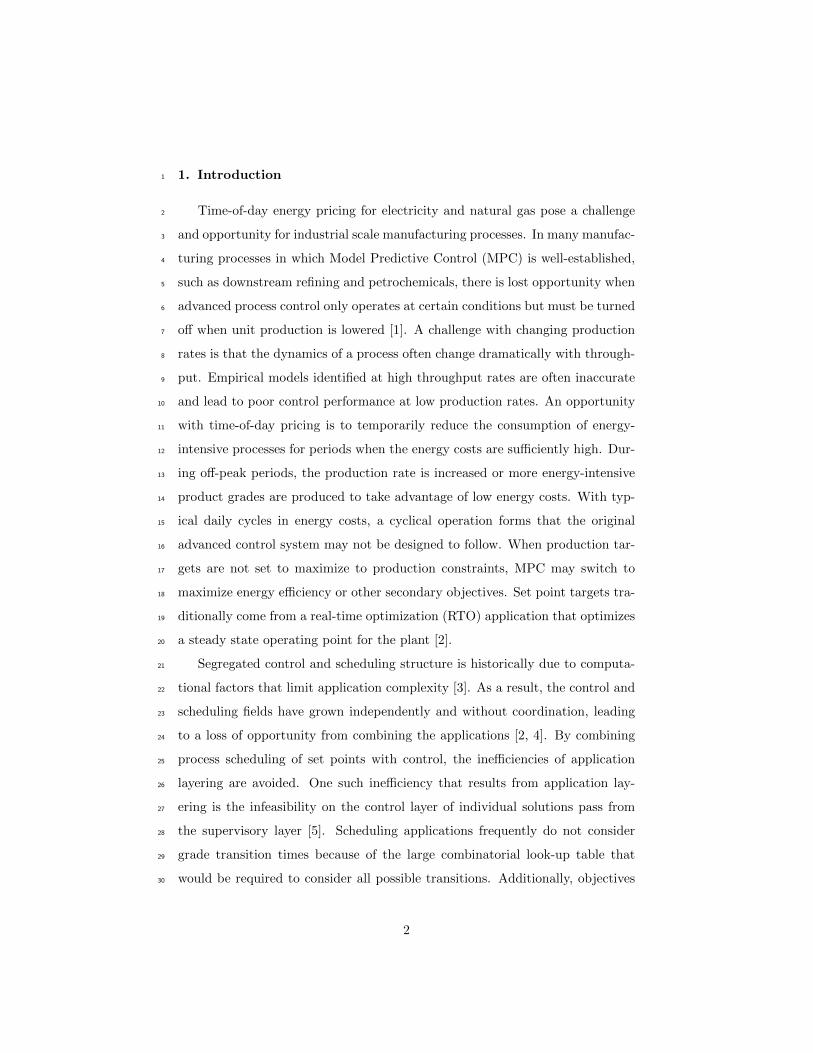
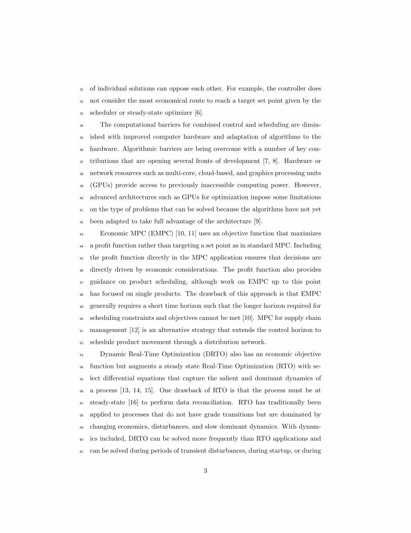
1. Introduction1
Time-of-day energy pricing for electricity and natural gas pose a challenge2
and opportunity for industrial scale manufacturing processes. In many manufac-3
turing processes in which Model Predictive Control (MPC) is well-established,4
such as downstream refining and petrochemicals, there is lost opportunity when5
advanced process control only operates at certain conditions but must be turned6
off when unit production is lowered [1]. A challenge with changing production7
rates is that the dynamics of a process often change dramatically with through-8
put. Empirical models identified at high throughput rates are often inaccurate9
and lead to poor control performance at low production rates. An opportunity10
with time-of-day pricing is to temporarily reduce the consumption of energy-11
intensive processes for periods when the energy costs are sufficiently high. Dur-12
ing off-peak periods, the production rate is increased or more energy-intensive13
product grades are produced to take advantage of low energy costs. With typ-14
ical daily cycles in energy costs, a cyclical operation forms that the original15
advanced control system may not be designed to follow. When production tar-16
gets are not set to maximize to production constraints, MPC may switch to17
maximize energy efficiency or other secondary objectives. Set point targets tra-18
ditionally come from a real-time optimization (RTO) application that optimizes19
a steady state operating point for the plant [2].20
Segregated control and scheduling structure is historically due to computa-21
tional factors that limit application complexity [3]. As a result, the control and22
scheduling fields have grown independently and without coordination, leading23
to a loss of opportunity from combining the applications [2, 4]. By combining24
process scheduling of set points with control, the inefficiencies of application25
layering are avoided. One such inefficiency that results from application lay-26
ering is the infeasibility on the control layer of individual solutions pass from27
the supervisory layer [5]. Scheduling applications frequently do not consider28
grade transition times because of the large combinatorial look-up table that29
would be required to consider all possible transitions. Additionally, objectives30
2
of individual solutions can oppose each other. For example, the controller does31
not consider the most economical route to reach a target set point given by the32
scheduler or steady-state optimizer [6].33
The computational barriers for combined control and scheduling are dimin-34
ished with improved computer hardware and adaptation of algorithms to the35
hardware. Algorithmic barriers are being overcome with a number of key con-36
tributions that are opening several fronts of development [7, 8]. Hardware or37
network resources such as multi-core, cloud-based, and graphics processing units38
(GPUs) provide access to previously inaccessible computing power. However,39
advanced architectures such as GPUs for optimization impose some limitations40
on the type of problems that can be solved because the algorithms have not yet41
been adapted to take full advantage of the architecture [9].42
Economic MPC (EMPC) [10, 11] uses an objective function that maximizes43
a profit function rather than targeting a set point as in standard MPC. Including44
the profit function directly in the MPC application ensures that decisions are45
directly driven by economic considerations. The profit function also provides46
guidance on product scheduling, although work on EMPC up to this point47
has focused on single products. The drawback of this approach is that EMPC48
generally requires a short time horizon such that the longer horizon required for49
scheduling constraints and objectives cannot be met [10]. MPC for supply chain50
management [12] is an alternative strategy that extends the control horizon to51
schedule product movement through a distribution network.52
Dynamic Real-Time Optimization (DRTO) also has an economic objective53
function but augments a steady state Real-Time Optimization (RTO) with se-54
lect differential equations that capture the salient and dominant dynamics of55
a process [13, 14, 15]. One drawback of RTO is that the process must be at56
steady-state [16] to perform data reconciliation. RTO has traditionally been57
applied to processes that do not have grade transitions but are dominated by58
changing economics, disturbances, and slow dominant dynamics. With dynam-59
ics included, DRTO can be solved more frequently than RTO applications and60
can be solved during periods of transient disturbances, during startup, or during61
3
shutdown periods. RTO calculations are typically performed every hour to ev-62
ery day while DRTO optimizes the transition between steady-state conditions.63
Like EMPC, DRTO does not manage multiple sequential product campaigns as64
a scheduler.65
Complete integration of scheduling and control requires an extended pre-66
diction horizon to plan the production sequence as well as near-term control67
actions. Two integration approaches are referred to as top-down (add control68
and dynamics to a scheduling application) or bottom-up (add scheduling to a69
control algorithm) [3]. An early top-down implementation includes differential70
and algebraic equations in the scheduling application [17]. Another method is71
the scale-bridging model (SBM) in which a simplified model of process dynamics72
is embedded in the scheduling application [18, 19, 20]. A benefit of this method73
is disturbance rejection [21]. Algorithms include Benders’ decomposition [22]74
for problems that have a large-scale structured form and Dinkelbach’s algorithm75
[23] for non-convex problems that require global optimization methods. Applica-76
tions of combined scheduling and control include batch processes [5, 24], polymer77
reactors [25], parallel Continuously Stirred Tank Reactors (CSTRs) [26], and an78
electrical grid that responds to current and future price signals [27].79
Variable electrical pricing incentivizes reduced consumption during peak80
hours [28]. It is desirable to match generation to consumption, but the adop-81
tion of more renewable energy requires producers and consumers to respond82
to price signals [29, 30, 31]. Energy producers may expose consumers to time-83
of-day pricing to discourage consumption during peak hours [32]. Scheduling84
operation of chemical processing [33, 34], oil refining [35], and air separation85
[36] are some examples of industrial units that can shed electrical load during86
peak hours, typically in the middle of the day. Many cooling-limited processes87
also operate more efficiently at night [34]. Periodic constraints can be used to88
optimize a typical daily cycle.89
Prior work in scheduling and control integration has been centered around90
slot-based, continuous-time scheduling formulations. The benefit of discrete-91
time formulation has been shown [34]. However, the non-linear discrete-time92
4
formulation proved computationally difficult. The purpose of this work is to93
restrict the dynamic model to linear form while capturing benefits of the inte-94
gration of scheduling and control. There is a large installed base of advanced95
controls that utilize linear models [1]. A unique aspect of this work is a time-96
scaling algorithm that adjusts the linear dynamic model based on residence97
time calculations with a theoretical foundation for first-order systems. The98
time-scaling approximation is applied to higher order, finite impulse response99
models that are common in industrial practice. These linear models are used in100
the combined scheduling and control application.101
2. Time-Scaling with First-Order Systems102
It is well known that linear MPC performance degrades with changes in the103
actual process time constant or gain [37]. This effect has been quantified for104
MPC where there is model mismatch in the time constant or gain of a first105
order system. A simple example is where the actual system is described by a106
single differential equation as τpdydt = −y + Kpu with a process time constant107
of τp = 1 and a process gain of Kp = 1. An MPC controller with objective108 ∑20i=1 |yi − 5| drives the response from a set point of 0 to 5. The controller109
model is similar to the process but with variable model time constant of τm and110
gain Km in the equation τmdydt = −y+Kmu. Common industrial practice is that111
acceptable MPC performance can be achieved with gain mismatch less than 30%112
(0.7 ≤ Km ≤ 1.3) and time constant mismatch less than 50% (0.5 ≤ τm ≤ 1.5)113
[37]. The dominant time constant for many industrial processes is characterized114
by the volume (V ) divided by the volumetric flowrate (q) as τp = V/q. The115
explicit solution to the first order equation is given by Equation 1.116
y[k + 1] = exp
(−∆t
τp
)y[k] +
(1− exp
(−∆t
τp
))Kp u[k] (1)
where y is the output, u is the input, k is the discrete time step, and t is the117
time. The integrated sum of absolute errors is computed for combinations of118
Km and τm, each between 0.1 and 5.0. The 3D contour plot shows the control119
5
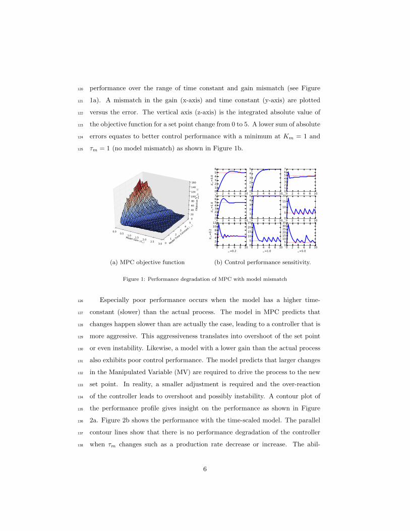
performance over the range of time constant and gain mismatch (see Figure120
1a). A mismatch in the gain (x-axis) and time constant (y-axis) are plotted121
versus the error. The vertical axis (z-axis) is the integrated absolute value of122
the objective function for a set point change from 0 to 5. A lower sum of absolute123
errors equates to better control performance with a minimum at Km = 1 and124
τm = 1 (no model mismatch) as shown in Figure 1b.125
Model Gain (Km)
0.00.5
1.01.5
2.02.5
3.0 Model Time Constant (τ
m)
0
1
2
3
4
5
Objective ∑ |y i
−5|
0
20
40
60
80
100
120
140
160
(a) MPC objective function
0 2 4 6 8 100123456
Km=3.0
0 2 4 6 8 100
1
2
3
4
5
0 2 4 6 8 1001234567
0 2 4 6 8 1001234567
Km=1.0
0 2 4 6 8 100
1
2
3
4
5
0 2 4 6 8 100
5
10
15
20
0 2 4 6 8 10τm=0.2
02468
1012
Km=0.2
0 2 4 6 8 10τm=1.0
0
5
10
15
20
25
0 2 4 6 8 10τm=5.0
05
101520253035
(b) Control performance sensitivity.
Figure 1: Performance degradation of MPC with model mismatch
Especially poor performance occurs when the model has a higher time-126
constant (slower) than the actual process. The model in MPC predicts that127
changes happen slower than are actually the case, leading to a controller that is128
more aggressive. This aggressiveness translates into overshoot of the set point129
or even instability. Likewise, a model with a lower gain than the actual process130
also exhibits poor control performance. The model predicts that larger changes131
in the Manipulated Variable (MV) are required to drive the process to the new132
set point. In reality, a smaller adjustment is required and the over-reaction133
of the controller leads to overshoot and possibly instability. A contour plot of134
the performance profile gives insight on the performance as shown in Figure135
2a. Figure 2b shows the performance with the time-scaled model. The parallel136
contour lines show that there is no performance degradation of the controller137
when τm changes such as a production rate decrease or increase. The abil-138
6
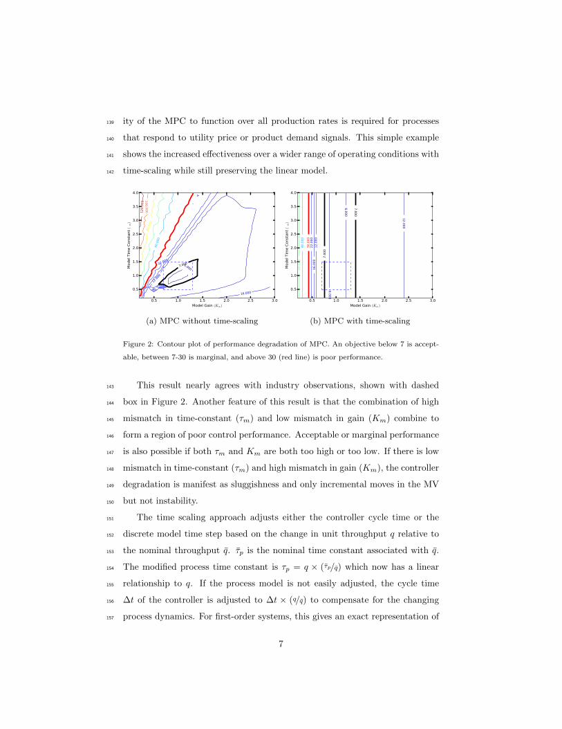
ity of the MPC to function over all production rates is required for processes139
that respond to utility price or product demand signals. This simple example140
shows the increased effectiveness over a wider range of operating conditions with141
time-scaling while still preserving the linear model.142
0.5 1.0 1.5 2.0 2.5 3.0Model Gain (Km)
0.5
1.0
1.5
2.0
2.5
3.0
3.5
4.0
Model Tim
e Constant (τm)
6.000
12.000
16.000
16.000
22.000
40.000
60.000
80.000
100.000
120.000
120.000
7.000
30.000
(a) MPC without time-scaling
0.5 1.0 1.5 2.0 2.5 3.0Model Gain (Km)
0.5
1.0
1.5
2.0
2.5
3.0
3.5
4.0
Model Tim
e Constant (τm)
6.000
6.000
12.000
12.000
16.000
22.000
40.000
60.000
7.000
7.000
30.000
(b) MPC with time-scaling
Figure 2: Contour plot of performance degradation of MPC. An objective below 7 is accept-
able, between 7-30 is marginal, and above 30 (red line) is poor performance.
This result nearly agrees with industry observations, shown with dashed143
box in Figure 2. Another feature of this result is that the combination of high144
mismatch in time-constant (τm) and low mismatch in gain (Km) combine to145
form a region of poor control performance. Acceptable or marginal performance146
is also possible if both τm and Km are both too high or too low. If there is low147
mismatch in time-constant (τm) and high mismatch in gain (Km), the controller148
degradation is manifest as sluggishness and only incremental moves in the MV149
but not instability.150
The time scaling approach adjusts either the controller cycle time or the151
discrete model time step based on the change in unit throughput q relative to152
the nominal throughput q. τp is the nominal time constant associated with q.153
The modified process time constant is τp = q × (τp/q) which now has a linear154
relationship to q. If the process model is not easily adjusted, the cycle time155
∆t of the controller is adjusted to ∆t × (q/q) to compensate for the changing156
process dynamics. For first-order systems, this gives an exact representation of157
7
the nonlinear dynamics without modifying the original linear model.158
3. Selective Time-Scaling159
Multi-variate and higher-order systems may have certain MV to CV relation-160
ships that are known to scale with changing unit throughput while others are161
invariant to throughput changes. Prior work has focused on decomposition of162
fast and slow dynamics [38] or variable time-delay of measurements [39, 40]. For163
systems with multiple MVs and CVs, only the relationships that are sensitive164
to throughput are scaled. These can be identified with a dynamic process sim-165
ulator or else by repeating plant identification tests at low and high production166
rates. A method to scale higher order systems is to transform the linear time-167
invariant (LTI) model into discrete form. In discrete form, the sampling time is168
scaled by (q/q) and resampled to preserve the overall model sampling time. As169
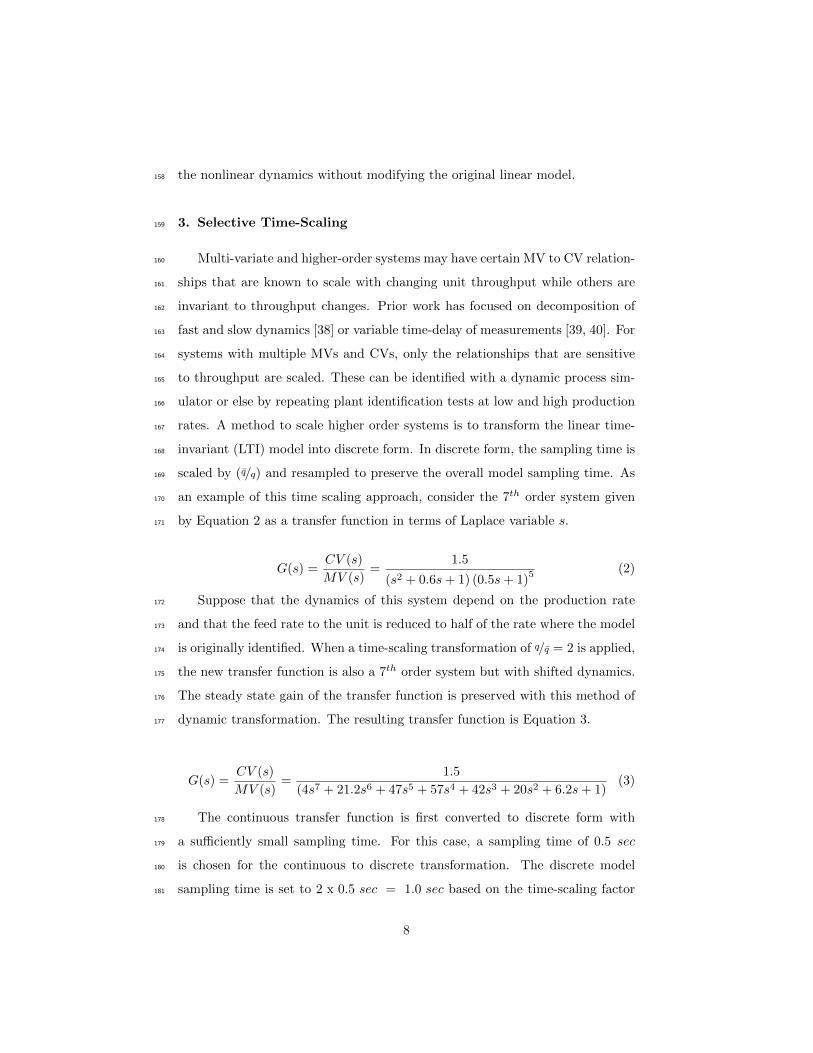
an example of this time scaling approach, consider the 7th order system given170
by Equation 2 as a transfer function in terms of Laplace variable s.171
G(s) =CV (s)
MV (s)=
1.5
(s2 + 0.6s+ 1) (0.5s+ 1)5 (2)
Suppose that the dynamics of this system depend on the production rate172
and that the feed rate to the unit is reduced to half of the rate where the model173
is originally identified. When a time-scaling transformation of q/q = 2 is applied,174
the new transfer function is also a 7th order system but with shifted dynamics.175
The steady state gain of the transfer function is preserved with this method of176
dynamic transformation. The resulting transfer function is Equation 3.177
G(s) =CV (s)
MV (s)=
1.5
(4s7 + 21.2s6 + 47s5 + 57s4 + 42s3 + 20s2 + 6.2s+ 1)(3)
The continuous transfer function is first converted to discrete form with178
a sufficiently small sampling time. For this case, a sampling time of 0.5 sec179
is chosen for the continuous to discrete transformation. The discrete model180
sampling time is set to 2 x 0.5 sec = 1.0 sec based on the time-scaling factor181
8
0 5 10 15 20 25 30 35 400
0.2
0.4
0.6
0.8
1
1.2
1.4
1.6
Original
Original Discrete
Time-Scaled
Time-Scaled Discrete
Time (seconds)
Ste
p R
esponse
Figure 3: Time-scaling of a 7th order system when the feed rate is reduced to half.
and then the model is resampled to 0.5 sec to be consistent with other unscaled182
MV/CV models. Continuous to discrete transformations and discrete model183
resampling for LTI models are standard methods [41] and are not repeated here184
for the sake of brevity. A graphical demonstration of this method is shown in185
Figure 3.186
4. Scheduling and Control Formulation187
An innovation of this work is to combine scheduling and control with lin-188
ear models and quadratic objective functions for fast solution with Quadratic189
Programming (QP) [42] or Nonlinear Programming (NLP) solvers. There are190
multiple methods for formulating tiered price structures. The focus of this work191
is on creating mathematical expressions that have continuous first and second192
derivatives and fit within the QP or a QP with Quadratic Constraint (QPQC)193
framework. In contrast, most modern scheduling applications utilize integer194
variables, often as binary decision variables. Including integers requires MILP195
or MINLP solvers, which are significantly slower and more complex.196
9
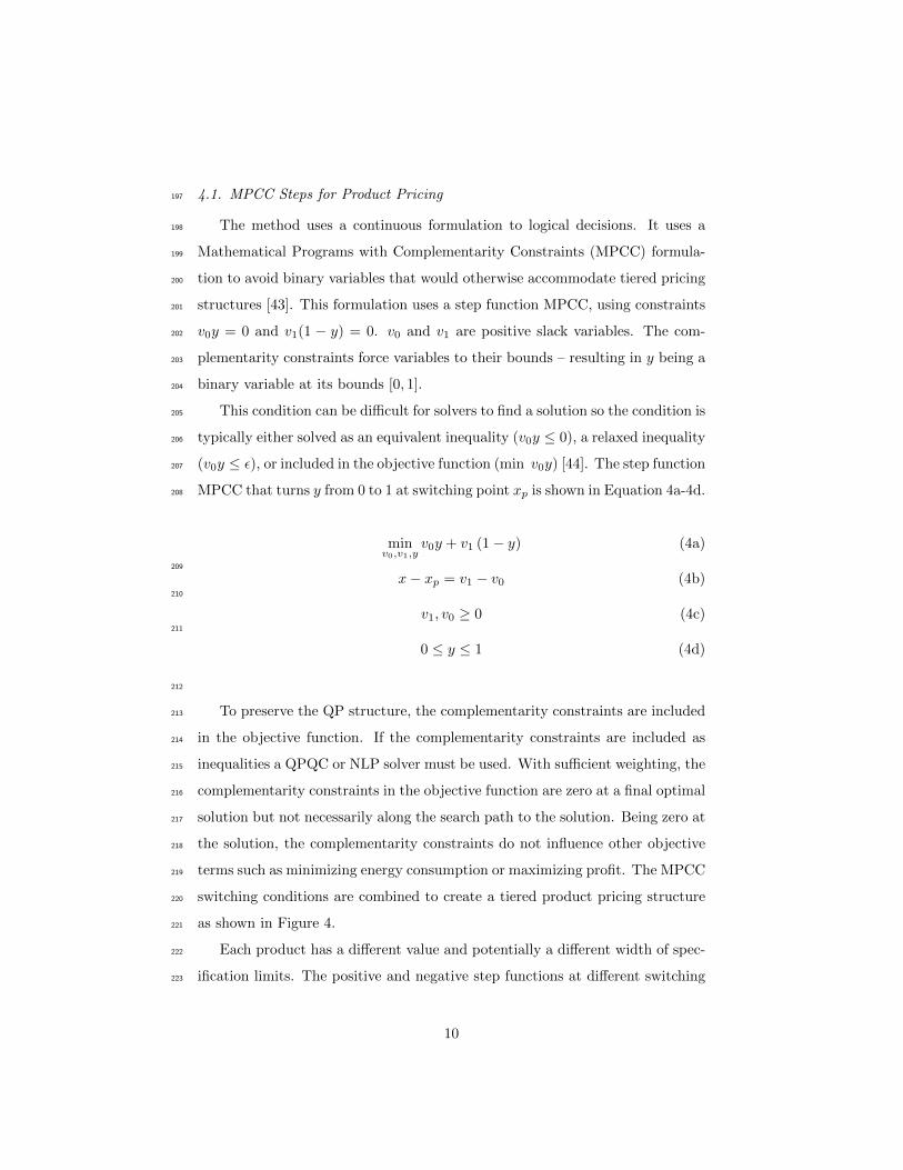
4.1. MPCC Steps for Product Pricing197
The method uses a continuous formulation to logical decisions. It uses a198
Mathematical Programs with Complementarity Constraints (MPCC) formula-199
tion to avoid binary variables that would otherwise accommodate tiered pricing200
structures [43]. This formulation uses a step function MPCC, using constraints201
v0y = 0 and v1(1 − y) = 0. v0 and v1 are positive slack variables. The com-202
plementarity constraints force variables to their bounds – resulting in y being a203
binary variable at its bounds [0, 1].204
This condition can be difficult for solvers to find a solution so the condition is205
typically either solved as an equivalent inequality (v0y ≤ 0), a relaxed inequality206
(v0y ≤ ε), or included in the objective function (min v0y) [44]. The step function207
MPCC that turns y from 0 to 1 at switching point xp is shown in Equation 4a-4d.208
minv0,v1,y
v0y + v1 (1− y) (4a)
209
x− xp = v1 − v0 (4b)210
v1, v0 ≥ 0 (4c)211
0 ≤ y ≤ 1 (4d)
212
To preserve the QP structure, the complementarity constraints are included213
in the objective function. If the complementarity constraints are included as214
inequalities a QPQC or NLP solver must be used. With sufficient weighting, the215
complementarity constraints in the objective function are zero at a final optimal216
solution but not necessarily along the search path to the solution. Being zero at217
the solution, the complementarity constraints do not influence other objective218
terms such as minimizing energy consumption or maximizing profit. The MPCC219
switching conditions are combined to create a tiered product pricing structure220
as shown in Figure 4.221
Each product has a different value and potentially a different width of spec-222
ification limits. The positive and negative step functions at different switching223
10
0 1 2 3 4 5-4
-2
0
2
4
Ste
p R
esponse
MPCC Step Function
0 1 2 3 4 5
Product Property
0
1
2
3
Pro
fit
A B C
Product Ranges
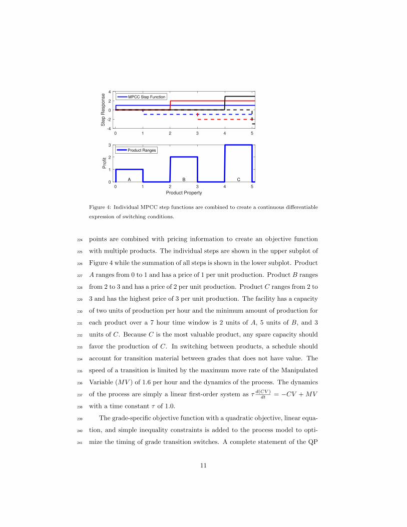
Figure 4: Individual MPCC step functions are combined to create a continuous differentiable
expression of switching conditions.
points are combined with pricing information to create an objective function224
with multiple products. The individual steps are shown in the upper subplot of225
Figure 4 while the summation of all steps is shown in the lower subplot. Product226
A ranges from 0 to 1 and has a price of 1 per unit production. Product B ranges227
from 2 to 3 and has a price of 2 per unit production. Product C ranges from 2 to228
3 and has the highest price of 3 per unit production. The facility has a capacity229
of two units of production per hour and the minimum amount of production for230
each product over a 7 hour time window is 2 units of A, 5 units of B, and 3231
units of C. Because C is the most valuable product, any spare capacity should232
favor the production of C. In switching between products, a schedule should233
account for transition material between grades that does not have value. The234
speed of a transition is limited by the maximum move rate of the Manipulated235
Variable (MV ) of 1.6 per hour and the dynamics of the process. The dynamics236
of the process are simply a linear first-order system as τ d(CV )dt = −CV + MV237
with a time constant τ of 1.0.238
The grade-specific objective function with a quadratic objective, linear equa-239
tion, and simple inequality constraints is added to the process model to opti-240
mize the timing of grade transition switches. A complete statement of the QP241
11
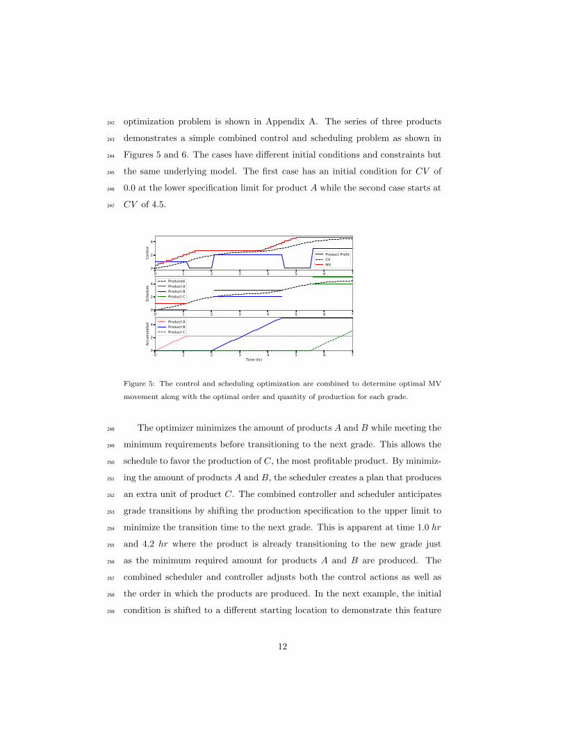
optimization problem is shown in Appendix A. The series of three products242
demonstrates a simple combined control and scheduling problem as shown in243
Figures 5 and 6. The cases have different initial conditions and constraints but244
the same underlying model. The first case has an initial condition for CV of245
0.0 at the lower specification limit for product A while the second case starts at246
CV of 4.5.247
0 1 2 3 4 5 6 70
2
4
Control
Product ProfitCVMV
0 1 2 3 4 5 6 70
2
4
Schedu
le
ProducedProduct AProduct BProduct C
0 1 2 3 4 5 6 7Time (hr)
0
2
4
Accumulated
Product AProduct BProduct C
Figure 5: The control and scheduling optimization are combined to determine optimal MV
movement along with the optimal order and quantity of production for each grade.
The optimizer minimizes the amount of products A and B while meeting the248
minimum requirements before transitioning to the next grade. This allows the249
schedule to favor the production of C, the most profitable product. By minimiz-250
ing the amount of products A and B, the scheduler creates a plan that produces251
an extra unit of product C. The combined controller and scheduler anticipates252
grade transitions by shifting the production specification to the upper limit to253
minimize the transition time to the next grade. This is apparent at time 1.0 hr254
and 4.2 hr where the product is already transitioning to the new grade just255
as the minimum required amount for products A and B are produced. The256
combined scheduler and controller adjusts both the control actions as well as257
the order in which the products are produced. In the next example, the initial258
condition is shifted to a different starting location to demonstrate this feature259
12
of the approach.260
The computational time is an important factor for control problems where261
the algorithm must return a solution within the cycle time necessary to rejected262
disturbances and maintain process stability. The fully discretized combined263
scheduling and control problem with 3 products and discrete time points has264
2730 variables, 1820 equations, and 910 degrees of freedom. The problem is265
solved on a Dell R815 server with an AMD Opteron 6276 Processor and 64266
GB of RAM. The problem requires 8.6 s to converge with the APOPT solver267
(version 1.0) or 4.0 s with the IPOPT solver (version 3.10). MPC commonly268
uses a warm-start from a prior solution to improve efficiency. With a warm-start269
from the prior time-step, the optimizer requires 0.5 s with APOPT and 3.0 s270
with IPOPT. Active-set solvers (such as APOPT) and interior point solvers271
(such as IPOPT) are both effective for large-scale MPC applications although272
interior point solvers have better performance as degrees of freedom increase [7].273
4.2. Dynamic Cyclic Schedule274
A common method to optimize a schedule in current practice is to place275
products on a fixed grade wheel where each product is visited sequentially in a276
rotation. The cyclic schedule visits all grades in a forward and then a reverse277
order to end up at the original grade and begin the cycle again. If there is a278
sudden demand for a particular grade out of sequence, the product wheel is still279
typically traversed in the grade wheel order but there may be a minimal amount280
of the less desirable grades in favor of the desired grade production. In some281
processes, such as polyolefin production, there are multiple versions of the grade282
wheel. One version of the grade wheel may include only commodity products283
while other wheels or sub-wheels may be a more complex cycles that include284
less frequently produced products.285
The contribution of this work is the discrete time, extended controller and286
scheduler that is also able to produce a cyclic schedule. However, this cyclic287
schedule is not fixed but adjusts the sequence of products automatically when288
updated economic or constraint information is available. The schedule and289
13
control action may update every controller cycle (e.g. every minute). Some290
constraints for scheduling are periodic boundary constraints where the final291
condition must be equal to the initial condition, contracted quantities that must292
be produced by a certain date or time, particular equipment limitation, or time-293
of-day transition constraints. An example of a time-of-day constraint is that294
certain grade transitions need start-up or shut-down of auxiliary equipment.295
A constraint may be that the grade transition should happen only during a296
weekday day-time shift where there is adequate operator support.297
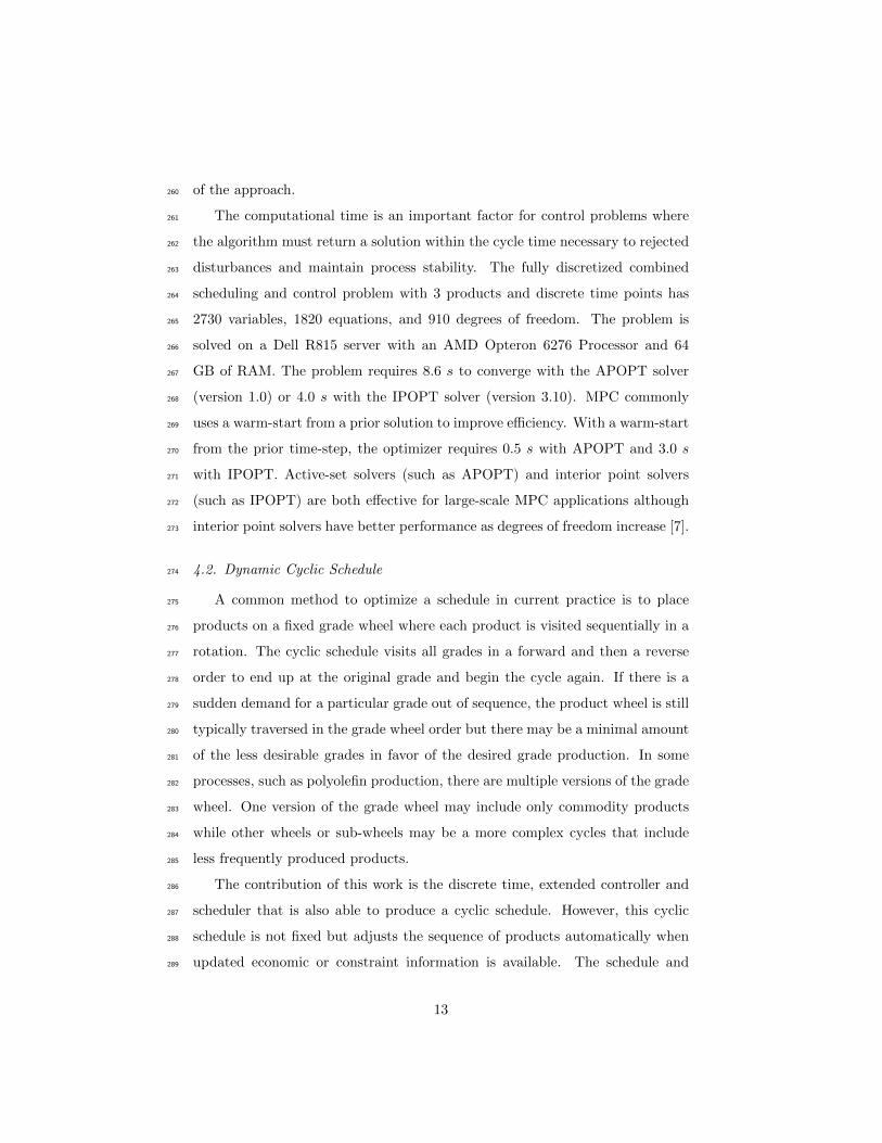
The prior example problem is augmented with intermediate production tar-298
gets and a periodic constraint. The scheduler and controller, shown in Figure299
6 produces an optimized schedule and control actions. It is a dynamic rather300
than a static grade wheel because the order of product production and quantity301
is re-optimized every cycle of the controller. The product order or quantity may302
change based on changing customer demand, price signals for electricity or feed303
costs, or disturbances that drive the system to a different state.304
0 2 4 6 8 100
2
4
6
Control Periodic
Constraint
Product ProfitCVMV
0 2 4 6 8 100
2
4
6
Sche
dule
ProducedProduct AProduct BProduct C
0 2 4 6 8 10Time (hr)
0
2
4
6
Accu
mulated Required
Deliveries
Product AProduct BProduct C
Figure 6: Optimized schedule with periodic condition, intermediate production targets, and
final production targets. The schedule and control actions adjust to meet constraints and
maximize profit (product C).
The optimized solution meets constraints as well as maximizes the produc-305
tion of product C, the highest value product. The intermediate constraints306
14
originate from contracted delivery times and storage capacity of a particular307
product. In this case, the storage capacity of all products is less than 5 units308
of production. This requires two deliveries of product B that are scheduled at309
two equally spaced intervals of 5 hrs. The production of product C exceeds310
the required delivery amount because it is the highest value product. Although311
the initial condition is at product C, the controller immediately targets product312
B to meet the required delivery of 5 units of production at 5 hrs. Without313
the periodic constraint, production of product C would be maximized before314
transitioning because the scheduler evaluates the alternative that a transition315
back to product C results in lost profit potential. However, with the required316
transition back to product C, the scheduler puts excess production of product317
C at the end.318
While this method is capable of producing cyclic schedules, the optimizer319
should begin from current conditions rather than steady-state product condi-320
tions to fully integrate control and scheduling. Cyclic schedules combined with321
online control may lead back to off-spec conditions because of disturbances or322
because the controller is in a transition. Instead, this method is better suited323
to a different set of constraints – production amounts and due dates. These324
constraints give more freedom to the optimizer so the economic objective will325
improve or be equal to the solution with periodic constraints.326
As with adding any constraint, there is potential to make the problem in-327
feasible. Multi-objective optimization statements, such as those used to refine328
a dynamic grade wheel sequence, can also be posed with a rank-ordered set of329
constraints with an explicit prioritization of objectives. The `1-norm dead-band330
formulation is discussed in more detail in [7] and related to combined schedul-331
ing and control production targets in Section 4.3. Posing the constraints as332
multi-objective penalties versus hard constraints allows the problem to remain333
feasible yet still meet the most important objectives in order of priority.334
15
4.3. Acceptable Range of Production Quantity335
One drawback to the prior examples is that all spare production capacity is336
typically placed on the highest value product. Over-production of any product337
can have the effect of lowering the selling price because of supply and demand338
market forces. In scheduling, there is often a range of production quantity that339
is acceptable instead of just a single hard limit. To accommodate this, the340
scheduling and control algorithm can use an `1-norm objective function to give341
a target region for the production quantity, rather than one specific hard limit.342
Equation 5 shows a generalized `1-norm control formulation used in this work.343
minx,CV,MV
Φ = wThiehi + wTloelo + xT cx +MV T cMV + ∆MV T c∆MV
s.t. 0 = f(d xd t , x,
dCVd t , CV,MV
)ehi ≥ x− dhielo ≥ dlo − x
(5)
In this formulation, Φ is the objective function, x is the production quantity344
per grade. Parameters wlo and whi are penalty matrices for solutions outside345
of the production target region. The slack variable elo and ehi define the error346
of the dead-band low and high limits. Parameters cx, cMV , and c∆MV are cost347
vectors for the production quantity (positive values minimize production within348
region, negative values maximize production within region), the MVs (positive349
values minimize MV quantities such as energy use, negative values maximize350
MV quantity such as pump speed correlated to higher efficiency), and change351
of MVs, respectively. The function f is an open-equation set of equations as352
functions of x, CV , MV , and time derivatives of x and CV . The demand353
targets dlo and dhi define lower and upper target limits for production.354
This range formulation is not used in this work but is presented to demon-355
strate one of many ways that this problem structure can be expanded to meet356
various scheduling needs.357
16
5. Application: Continuously Stirred Tank Reactor358
A continuously stirred tank reactor (CSTR) is a common benchmark used359
in nonlinear model predictive control and scheduling applications [34, 3, 16].360
This nonlinear application is used to demonstrate the strength of the approach361
to time-scale based on throughput and combined scheduling & control.362
The linear time-scaled model changes dynamics based on reactor flow rate,363
allowing linear MPC to be used instead of nonlinear MPC. The multi-product364
scheduling objective is used instead of a simple target tracking to combine the365
scheduling and control into one application. Rapid convergence is ensured with a366
linear model and quadratic objective because the problem is convex and because367
QP solvers are efficient for large-scale systems.368
The CSTR application is highly nonlinear because of an exothermic reaction369
that has the potential to cause rapid reaction of stored reactant and thereby370
cause a temperature run-away. The CSTR shares characteristics of many in-371
dustrial processes such as polymer reactors or many refining processes but with372
much simpler mathematics that are amenable to demonstrating a new approach373
for control and scheduling. The liquid full reactor is used to convert compounds374
A ⇒ B with constant liquid density (ρ) and heat capacity (Cp) as shown in375
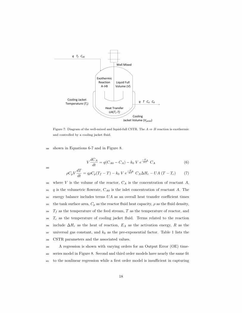
Figure 7.376
The reaction kinetics are first order and irreversible. Reaction of A to B is377
exothermic with the potential for temperature run-away because of the exponen-378
tial dependence of reaction rate on temperature, typical of an Arrhenius form379
for reaction rates. The reactor is well-mixed with reactor concentration and380
temperature equally distributed and also equal to the outlet measured values.381
The reactor temperature is regulated with a cooling jacket liquid temperature,382
Tc. The cooling jacket temperature is normally regulated by adjusting the rate383
of cooling or the coolant flow rate but in this model the jacket temperature384
is assumed to be controlled directly and the dynamics are approximated by a385
maximum rate of change.386
The dynamics of the CSTR are dictated by a species and energy balance as387
17
q Tf CA0
Cooling Jacket Temperature (Tc)
q T CA CB
ExothermicReaction
A B
CoolingJacket Volume (Vjacket)
Heat TransferUA(Tc-T)
Liquid FullVolume (V)
Well Mixed
Figure 7: Diagram of the well-mixed and liquid-full CSTR. The A ⇒ B reaction is exothermic
and controlled by a cooling jacket fluid.
shown in Equations 6-7 and in Figure 8.388
VdCAdt
= q(CA0 − CA)− k0 V e−EART CA (6)
389
ρCpVdT
dt= qρCp(Tf − T )− k0 V e
−EART CA∆Hr − UA (T − Tc) (7)
where V is the volume of the reactor, CA is the concentration of reactant A,390
q is the volumetric flowrate, CA0 is the inlet concentration of reactant A. The391
energy balance includes terms UA as an overall heat transfer coefficient times392
the tank surface area, Cp as the reactor fluid heat capacity, ρ as the fluid density,393
Tf as the temperature of the feed stream, T as the temperature of reactor, and394
Tc as the temperature of cooling jacket fluid. Terms related to the reaction395
include ∆Hr as the heat of reaction, EA as the activation energy, R as the396
universal gas constant, and k0 as the pre-exponential factor. Table 1 lists the397
CSTR parameters and the associated values.398
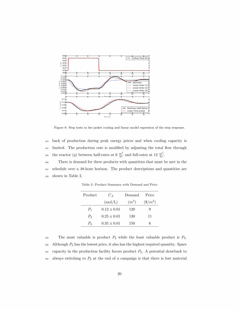
A regression is shown with varying orders for an Output Error (OE) time-399
series model in Figure 8. Second and third order models have nearly the same fit400
to the nonlinear regression while a first order model is insufficient in capturing401
18
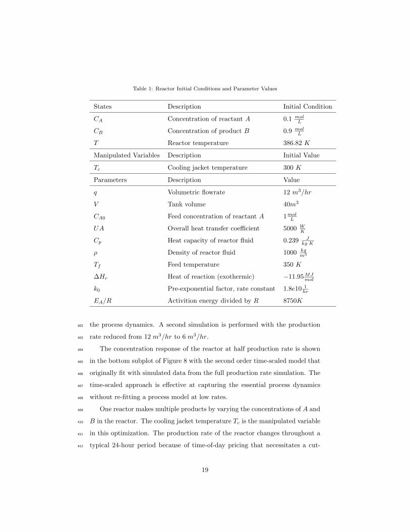
Table 1: Reactor Initial Conditions and Parameter Values
States Description Initial Condition
CA Concentration of reactant A 0.1 molL
CB Concentration of product B 0.9 molL
T Reactor temperature 386.82 K
Manipulated Variables Description Initial Value
Tc Cooling jacket temperature 300 K
Parameters Description Value
q Volumetric flowrate 12 m3/hr
V Tank volume 40m3
CA0 Feed concentration of reactant A 1molL
UA Overall heat transfer coefficient 5000 WK
Cp Heat capacity of reactor fluid 0.239 Jkg K
ρ Density of reactor fluid 1000 kgm3
Tf Feed temperature 350 K
∆Hr Heat of reaction (exothermic) −11.95MJmol
k0 Pre-exponential factor, rate constant 1.8e10 1hr
EA/R Activition energy divided by R 8750K
the process dynamics. A second simulation is performed with the production402
rate reduced from 12 m3/hr to 6 m3/hr.403
The concentration response of the reactor at half production rate is shown404
in the bottom subplot of Figure 8 with the second order time-scaled model that405
originally fit with simulated data from the full production rate simulation. The406
time-scaled approach is effective at capturing the essential process dynamics407
without re-fitting a process model at low rates.408
One reactor makes multiple products by varying the concentrations of A and409
B in the reactor. The cooling jacket temperature Tc is the manipulated variable410
in this optimization. The production rate of the reactor changes throughout a411
typical 24-hour period because of time-of-day pricing that necessitates a cut-412
19
0 2 4 6 8 10 12 14299
300
301
302
303
304
305
306
Tc(K
)
Cooling Temp (K)
0 2 4 6 8 10 12 14Time (hr)
0.0650.0700.0750.0800.0850.0900.0950.1000.1050.110
CA
(mol/L
)
NonlinearLinear Order (1)Linear Order (2)Linear Order (3)
0 2 4 6 8 10 12 14Time (hr)
0.06
0.07
0.08
0.09
0.10
0.11
CA
(mol/L
)
Nonlinear (Half Rates)Linear Time-Scaled
Figure 8: Step tests in the jacket cooling and linear model regression of the step response.
back of production during peak energy prices and when cooling capacity is413
limited. The production rate is modified by adjusting the total flow through414
the reactor (q) between half-rates at 6 m3
hr and full-rates at 12 m3
hr .415
There is demand for three products with quantities that must be met in the416
schedule over a 48-hour horizon. The product descriptions and quantities are417
shown in Table 2.418
Table 2: Product Summary with Demand and Price
Product CA Demand Price
(mol/L) (m3) ($/m3)
P1 0.12± 0.01 120 9
P2 0.25± 0.01 130 11
P3 0.35± 0.01 150 6
The most valuable is product P2 while the least valuable product is P3.419
Although P3 has the lowest price, it also has the highest required quantity. Spare420
capacity in the production facility favors product P2. A potential drawback to421
always switching to P2 at the end of a campaign is that there is lost material422
20
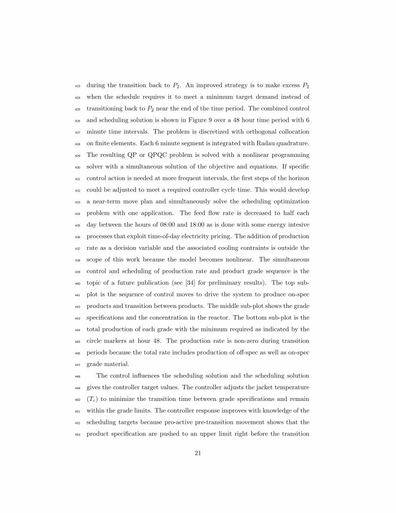
during the transition back to P2. An improved strategy is to make excess P2423
when the schedule requires it to meet a minimum target demand instead of424
transitioning back to P2 near the end of the time period. The combined control425
and scheduling solution is shown in Figure 9 over a 48 hour time period with 6426
minute time intervals. The problem is discretized with orthogonal collocation427
on finite elements. Each 6 minute segment is integrated with Radau quadrature.428
The resulting QP or QPQC problem is solved with a nonlinear programming429
solver with a simultaneous solution of the objective and equations. If specific430
control action is needed at more frequent intervals, the first steps of the horizon431
could be adjusted to meet a required controller cycle time. This would develop432
a near-term move plan and simultaneously solve the scheduling optimization433
problem with one application. The feed flow rate is decreased to half each434
day between the hours of 08:00 and 18:00 as is done with some energy intesive435
processes that exploit time-of-day electricity pricing. The addition of production436
rate as a decision variable and the associated cooling contraints is outside the437
scope of this work because the model becomes nonlinear. The simultaneous438
control and scheduling of production rate and product grade sequence is the439
topic of a future publication (see [34] for preliminary results). The top sub-440
plot is the sequence of control moves to drive the system to produce on-spec441
products and transition between products. The middle sub-plot shows the grade442
specifications and the concentration in the reactor. The bottom sub-plot is the443
total production of each grade with the minimum required as indicated by the444
circle markers at hour 48. The production rate is non-zero during transition445
periods because the total rate includes production of off-spec as well as on-spec446
grade material.447
The control influences the scheduling solution and the scheduling solution448
gives the controller target values. The controller adjusts the jacket temperature449
(Tc) to minimize the transition time between grade specifications and remain450
within the grade limits. The controller response improves with knowledge of the451
scheduling targets because pro-active pre-transition movement shows that the452
product specification are pushed to an upper limit right before the transition453
21
0 10 20 30 40
260
280
300
T c(K)
Jacket Temperature
0 10 20 30 400.0
0.1
0.2
0.3
0.4
0.5
Sche
dule
9/m3
11/m3
6/m3ConcentrationProduct 3Product 2Product 1
0 10 20 30 40Time (hr)
0
50
100
150
200
Prod
uctio
n
Product 1 > 120 (m3)Product 2 > 130 (m3)Product 3 > 150 (m3)Feed Flow Rate (m3/hr)
Figure 9: Combined control and schedule optimization results.
begins. One factor that affects the schedule is the speed of the transition from454
one product to another. The control dynamics are due to limitations in the455
manipulated variable movement and the process dynamics affecting the speed456
of attaining concentration range. The speed of the control response is factored457
into the schedule as lost production time when transition (off-spec) material is458
produced. Blending of transition material is one strategy to dilute the off-test459
material in prime products. This strategy is not considered in this approach460
but could be included as a constraint on the amount of reblend fraction that is461
allowed in the final product.462
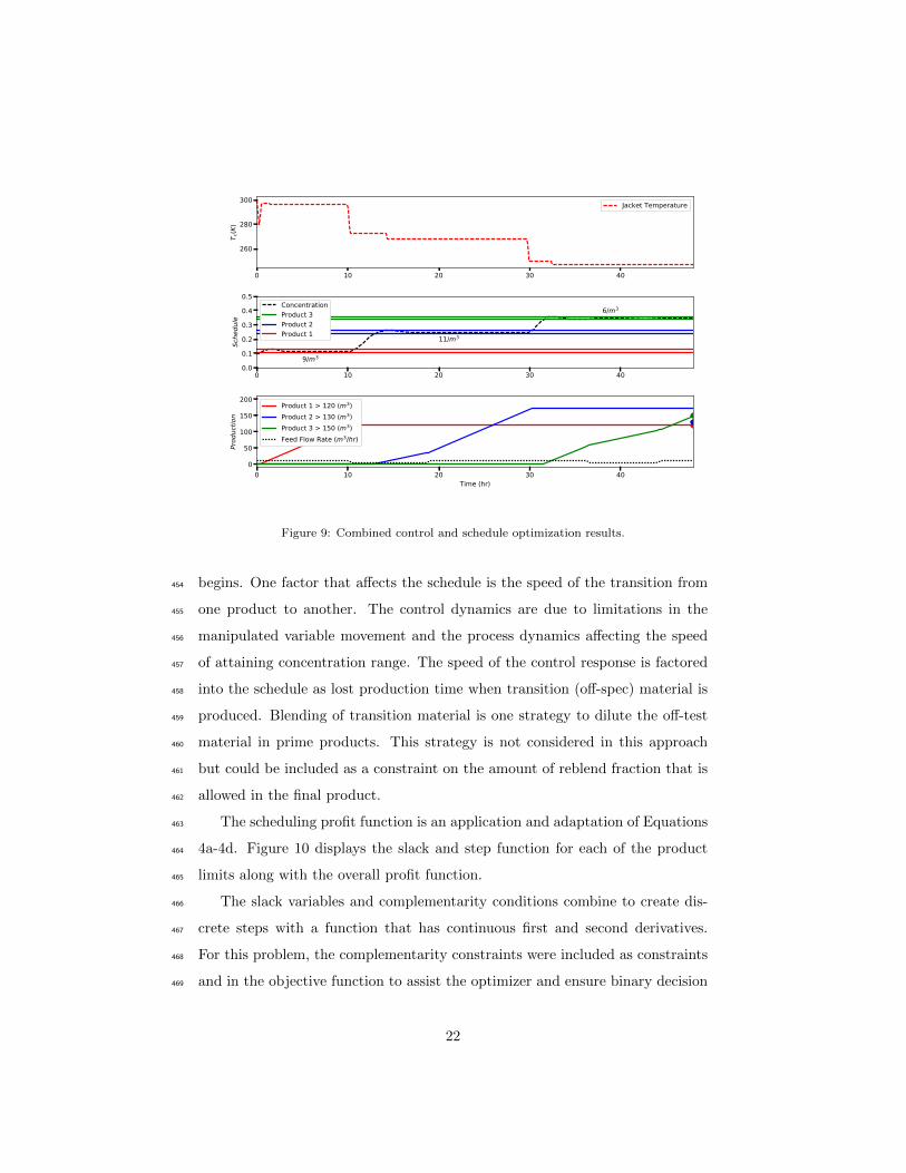
The scheduling profit function is an application and adaptation of Equations463
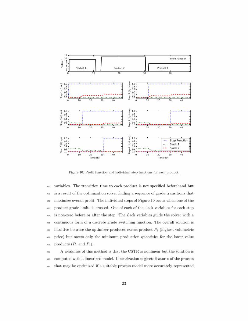
4a-4d. Figure 10 displays the slack and step function for each of the product464
limits along with the overall profit function.465
The slack variables and complementarity conditions combine to create dis-466
crete steps with a function that has continuous first and second derivatives.467
For this problem, the complementarity constraints were included as constraints468
and in the objective function to assist the optimizer and ensure binary decision469
22
0 10 20 30 4002468
1012
Profit/m
3 Profit Function
Product 1 Product 2 Product 3
0 10 20 30 400.00.20.40.60.81.0
Step 1 (P1 up)
0 10 20 30 400.00.20.40.60.81.0
Step 2 (P1 down)
0 10 20 30 400.00.20.40.60.81.0
Step 3 (P2 up)
0 10 20 30 400.00.20.40.60.81.0
Step 4 (P2 down)
0 10 20 30 40Time (hr)
0.00.20.40.60.81.0
Step 5 (P3 up)
0 10 20 30 40Time (hr)
0.00.20.40.60.81.0
Step 6 (P3 down)
Step FunctionSlack 1Slack 2
Figure 10: Profit function and individual step functions for each product.
variables. The transition time to each product is not specified beforehand but470
is a result of the optimization solver finding a sequence of grade transitions that471
maximize overall profit. The individual steps of Figure 10 occur when one of the472
product grade limits is crossed. One of each of the slack variables for each step473
is non-zero before or after the step. The slack variables guide the solver with a474
continuous form of a discrete grade switching function. The overall solution is475
intuitive because the optimizer produces excess product P2 (highest volumetric476
price) but meets only the minimum production quantities for the lower value477
products (P1 and P3).478
A weakness of this method is that the CSTR is nonlinear but the solution is479
computed with a linearized model. Linearization neglects features of the process480
that may be optimized if a suitable process model more accurately represented481
23
the physical process. A key contribution of this work is that the solution to482
the combined control and scheduling problem is relatively computationally in-483
expensive in comparison to a full nonlinear solution. In this case, the linearized484
model with time-scaling has a total of 22, 048 variables and 16, 640 equations485
and is solved on a Dell R815 with an AMD Opteron 6276 Processor and 64486
GB of RAM. After initialization, the problem requires 23.7 s to converge with487
the IPOPT solver. This is representative of the cycle time of the application488
as it repeatedly solves to reject disturbances and as new objective information489
or demand constraint information is available. This speed, coupled with the490
inclusion of a process model sufficient for control, allows this formulation to be491
utilized for on-line control, on top of providing an advanced schedule. This is492
the epitome of combining scheduling and control – a fully unified optimization493
that can replace both layers.494
A nonlinear version of this application is future work that will be reported495
in a subsequent publication. A key difference with the full nonlinear solution496
is that the solution in this work is several orders of magitude faster because497
of the quadratic objective and linear time-scaled model. Although combined498
scheduling and control with linear models or feedback linearization does not499
always accurately predict a highly nonlinear system, the linearized solution is a500
valuable starting point to initialize a nonlinear solution. Also, many processes501
are not highly nonlinear and this approach is likely suitable for systems that are502
already controlled with linear MPC.503
6. Conclusion504
A combined scheduling and control application is enabled by an MPCC ob-505
jective function, discrete-time, and linear time-scaling of process dynamics based506
on production rate changes. The objective of this work is to extend traditional507
linear MPC applications with a scheduling objective that allows for rapid con-508
vergence for real-time applications. One drawback of this work is that nonlin-509
earities are not included in the application. These nonlinearities are the subject510
24
of future work. The method is tested on a CSTR application that includes three511
grades over a 48 hour time horizon with 6 minute time intervals. The embed-512
ded controller simulates realistic transition times between each of the products.513
The scheduling objective determines the order and quantity of production at514
each grade even with half-rate reduction during peak electricity demand. The515
formulation is sufficiently fast enough, and includes enough process dynamics,516
to be utilized in on-line control. This presents a fully unified optimization that517
fulfills the roles of, and can replace, both control and scheduling for a compa-518
rable system. Although the method is demonstrated on the CSTR application,519
this formulation can be applied to other systems by replacing the model, pricing520
structure, and constraints of the scheduler.521
Acknowledgments522
Financial support from the NSF Award 1547110, EAGER: Cyber-Manufacturing523
with Multi-echelon Control and Scheduling, is gratefully acknowledged.524
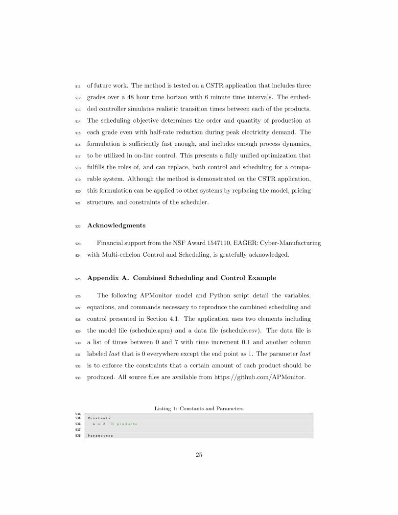
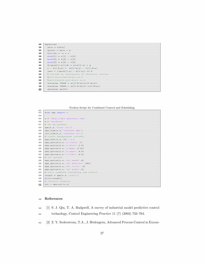
Appendix A. Combined Scheduling and Control Example525
The following APMonitor model and Python script detail the variables,526
equations, and commands necessary to reproduce the combined scheduling and527
control presented in Section 4.1. The application uses two elements including528
the model file (schedule.apm) and a data file (schedule.csv). The data file is529
a list of times between 0 and 7 with time increment 0.1 and another column530
labeled last that is 0 everywhere except the end point as 1. The parameter last531
is to enforce the constraints that a certain amount of each product should be532
produced. All source files are available from https://github.com/APMonitor.533
Listing 1: Constants and Parameters5341 C o n s t a n t s535
2 n = 3 % products536
3537
4 P a r a m e t e r s538
25
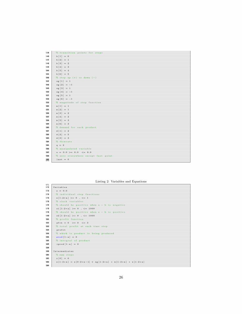
5 % t r a n s i t i o n po int s f o r s t eps539
6 b [ 1 ] = 0540
7 b [ 2 ] = 1541
8 b [ 3 ] = 2542
9 b [ 4 ] = 3543
10 b [ 5 ] = 4544
11 b [ 6 ] = 5545
12 % step up (+) or down (−)546
13 s g [ 1 ] = 1547
14 s g [ 2 ] = −1548
15 s g [ 3 ] = 1549
16 s g [ 4 ] = −1550
17 s g [ 5 ] = 1551
18 s g [ 6 ] = −1552
19 % magnitude o f s tep funct i on553
20 m [ 1 ] = 1554
21 m [ 2 ] = 1555
22 m [ 3 ] = 2556
23 m [ 4 ] = 2557
24 m [ 5 ] = 3558
25 m [ 6 ] = 3559
26 % demand f o r each product560
27 d [ 1 ] = 2561
28 d [ 2 ] = 5562
29 d [ 3 ] = 3563
30 % f l owra t e564
31 q = 2565
32 % manipulated va r i ab l e566
33 u = 0.0 >= 0.0 <= 8.0567
34 % zero everywhere except l a s t point568
35 l a s t = 0569570
Listing 2: Variables and Equations5711 V a r i a b l e s572
2 x = 0.0573
3 % ind i v i dua l step func t i on s574
4 w [ 1 : 2 ∗ n ] >= 0 , <= 1575
5 % s l a ck va r i a b l e s576
6 % should be p o s i t i v e when x − b i s negat ive577
7 s 1 [ 1 : 2 ∗ n ] >= 0 , <= 1000578
8 % should be p o s i t i v e when x − b i s p o s i t i v e579
9 s 2 [ 1 : 2 ∗ n ] >= 0 , <= 1000580
10 % p r o f i t funct i on581
11 p f c n = 0 >= 0 <= 3582
12 % to t a l p r o f i t at each time step583
13 p r o f i t584
14 % which i s product i s being produced585
15 prod [ 1 : n ] = 0586
16 % i n t e g r a l o f product587
17 i p r o d [ 1 : n ] = 0588
18589
19 I n t e r m e d i a t e s590
20 % sum steps591
21 z [ 0 ] = 0592
22 z [ 1 : 2 ∗ n ] = z [ 0 : 2 ∗ n −1] + s g [ 1 : 2 ∗ n ] ∗ m [ 1 : 2 ∗ n ] ∗ w [ 1 : 2 ∗ n ]593
23594
26
24 E q u a t i o n s595
25 p f c n = z [ 2∗ n ]596
26 p r o f i t = p f c n ∗ q597
27 d ( x ) / d t = −x + u598
28 prod [ 1 ] = w [ 1 ] − w [ 2 ]599
29 prod [ 2 ] = w [ 3 ] − w [ 4 ]600
30 prod [ 3 ] = w [ 5 ] − w [ 6 ]601
31 d ( i p r o d [ 1 : n ] ) / d t = prod [ 1 : n ] ∗ q602
32 x − b [ 1 : 2 ∗ n ] = s 2 [ 1 : 2 ∗ n ] − s 1 [ 1 : 2 ∗ n ]603
33 l a s t ∗ ( i p r o d [ 1 : n ] − d [ 1 : n ] ) >= 0604
34 % inc lude as a l t e r n a t i v e to ob j e c t i v e ve r s i on605
35 %s1 [ 1 : 2 ∗ n ] ∗ (w[ 1 : 2 ∗ n ] ) <= 0606
36 %s2 [ 1 : 2 ∗ n]∗(1−w[ 1 : 2 ∗ n ] ) <= 0607
37 m i n i m i z e 10000 ∗ s 1 [ 1 : 2 ∗ n ] ∗ ( w [ 1 : 2 ∗ n ] )608
38 m i n i m i z e 10000 ∗ s 2 [ 1 : 2 ∗ n ]∗(1− w [ 1 : 2 ∗ n ] )609
39 m a x i m i z e p r o f i t610611
Python Script for Combined Control and Scheduling612
from a p m import ∗613
614
s = ' http :// byu . apmonitor . com '615
a = ' products '616
# set up problem617
a p m ( s , a , ' c l e a r a l l ' )618
a p m _ l o a d ( s , a , ' schedule . apm ' )619
c s v _ l o a d ( s , a , ' schedule . csv ' )620
# crea t e manipulated va r i ab l e621
a p m _ i n f o ( s , a , 'MV' , 'u ' )622
a p m _ o p t i o n ( s , a , 'u . s ta tu s ' , 1 )623
a p m _ o p t i o n ( s , a , 'u . dcost ' , 1 . 0 )624
a p m _ o p t i o n ( s , a , 'u . dmax ' , 0 . 16 )625
a p m _ o p t i o n ( s , a , 'u . upper ' , 8 . 0 )626
a p m _ o p t i o n ( s , a , 'u . lower ' , 0 . 0 )627
# set opt ions628
a p m _ o p t i o n ( s , a , ' nlc . imode ' , 6 )629
a p m _ o p t i o n ( s , a , ' nlc . max iter ' ,200)630
a p m _ o p t i o n ( s , a , ' nlc . s o l v e r ' , 3 )631
a p m _ o p t i o n ( s , a , ' nlc . nodes ' , 2 )632
# so lve combined schedu l ing and cont ro l633
o u t p u t = a p m ( s , a , ' s o l v e ' )634
pr in t ( o u t p u t )635
# r e t r i e v e s o l u t i on636
s o l = a p m _ s o l ( s , a )637638
References639
[1] S. J. Qin, T. A. Badgwell, A survey of industrial model predictive control640
technology, Control Engineering Practice 11 (7) (2003) 733–764.641
[2] Z. Y. Soderstrom, T.A., J. Hedengren, Advanced Process Control in Exxon-642
27
Mobil Chemical Company: Successes and Challenges, in: CAST Division,643
AIChE National Meeting, Salt Lake City, UT, 2010.644
[3] M. Baldea, I. Harjunkoski, Integrated production scheduling and process645
control: A systematic review, Computers & Chemical Engineering 71646
(2014) 377–390. doi:10.1016/j.compchemeng.2014.09.002.647
[4] T. Backx, O. Bosgra, W. Marquardt, Integration of model predictive con-648
trol and optimization of processes, in: IFAC Symposium: Advanced Con-649
trol of Chemical Processes, Pisa, Italy, pp. 249–260.650
[5] E. Capon-Garcıa, G. Guillen-Gosalbez, A. Espuna, Integrating pro-651
cess dynamics within batch process scheduling via mixed-integer dy-652
namic optimization, Chemical Engineering Science 102 (2013) 139–150.653
doi:10.1016/j.ces.2013.07.039.654
URL http://dx.doi.org/10.1016/j.ces.2013.07.039655
[6] I. Harjunkoski, R. Nystrom, A. Horch, Integration of scheduling and656
control-Theory or practice?, Computers & Chemical Engineering 33 (2009)657
1909–1918. doi:10.1016/j.compchemeng.2009.06.016.658
[7] J. D. Hedengren, R. A. Shishavan, K. M. Powell, T. F. Edgar, Nonlinear659
modeling, estimation and predictive control in {APMonitor}, Computers660
& Chemical Engineering 70 (2014) 133 – 148, manfred Morari Special661
Issue. doi:10.1016/j.compchemeng.2014.04.013.662
URL http://www.sciencedirect.com/science/article/pii/663
S0098135414001306664
[8] F. V. Lima, M. R. Rajamani, T. A. Soderstrom, J. B. Rawlings, Covariance665
and State Estimation of Weakly Observable Systems: Application to Poly-666
merization Processes, IEEE Transactions on Control Systems Technology667
21 (4) (2013) 1249–1257. doi:10.1109/TCST.2012.2200296.668
[9] W. Ma, G. Agrawal, An integer programming framework for optimizing669
28
shared memory use on gpus, in: 2010 International Conference on High670
Performance Computing, 2010, pp. 1–10. doi:10.1109/HIPC.2010.5713187.671
[10] M. Ellis, H. Durand, P. D. Christofides, A tutorial review of economic model672
predictive control methods, Journal of Process Control 24 (8) (2014) 1156–673
1178. doi:10.1016/j.jprocont.2014.03.010.674
URL http://dx.doi.org/10.1016/j.jprocont.2014.03.010675
[11] D. Angeli, R. Amrit, J. B. Rawlings, On Average Performance and Stability676
of Economic Model Predictive Control, IEEE Transactions on Automatic677
Control 57 (7) (2012) 1615–1626. doi:10.1109/TAC.2011.2179349.678
[12] K. Subramanian, J. B. Rawlings, C. T. Maravelias, Economic679
model predictive control for inventory management in supply680
chains, Computers & Chemical Engineering 64 (2014) 71–80.681
doi:http://dx.doi.org/10.1016/j.compchemeng.2014.01.003.682
URL http://www.sciencedirect.com/science/article/pii/683
S0098135414000052684
[13] K. V. Pontes, I. J. Wolf, M. Embirucu, W. Marquardt, Dynamic Real-Time685
Optimization of Industrial Polymerization Processes with Fast Dynamics,686
Industrial & Engineering Chemistry Research 54 (47) (2015) 11881–11893.687
doi:10.1021/acs.iecr.5b00909.688
URL http://pubs.acs.org/doi/10.1021/acs.iecr.5b00909689
[14] I. Harjunkoski, C. T. Maravelias, P. Bongers, P. M. Castro, S. Engell,690
I. E. Grossmann, J. Hooker, C. Mendez, G. Sand, J. Wassick, Scope691
for industrial applications of production scheduling models and solu-692
tion methods, Computers & Chemical Engineering 62 (2014) 161–193.693
doi:10.1016/j.compchemeng.2013.12.001.694
URL http://dx.doi.org/10.1016/j.compchemeng.2013.12.001695
[15] L. Biegler, X. Yang, G. Fischer, Advances in sensitivity-based nonlinear696
model predictive control and dynamic real-time optimization, Journal of697
29
Process Control 30 (2015) 104–116. doi:10.1016/j.jprocont.2015.02.001.698
URL http://linkinghub.elsevier.com/retrieve/pii/699
S0959152415000281700
[16] J. Kelly, J. Hedengren, A steady-state detection (SSD) algorithm to detect701
non-stationary drifts in processes, Journal of Process Control 23 (3) (2013)702
326–331.703
[17] A. Flores-Tlacuahuac, I. E. Grossmann, Simultaneous Cyclic Scheduling704
and Control of a Multiproduct CSTR, Industrial & Engineering Chemistry705
Research 45 (20) (2006) 6698–6712. doi:10.1021/ie051293d.706
URL http://pubs.acs.org/doi/abs/10.1021/ie051293d707
[18] M. Baldea, J. Du, J. Park, I. Harjunkoski, Integrated production schedul-708
ing and model predictive control of continuous processes, AIChE Journal709
61 (12) (2015) 4179–4190. doi:10.1002/aic.14951.710
URL http://doi.wiley.com/10.1002/aic.14951711
[19] J. Du, J. Park, I. Harjunkoski, M. Baldea, A time scale-712
bridging approach for integrating production scheduling and pro-713
cess control, Computers & Chemical Engineering 79 (2015) 59–69.714
doi:10.1016/j.compchemeng.2015.04.026.715
URL http://linkinghub.elsevier.com/retrieve/pii/716
S0098135415001271717
[20] M. Baldea, C. R. Touretzky, J. Park, R. C. Pattison, Handling Input Dy-718
namics in Integrated Scheduling and Control, in: 2016 IEEE International719
Conference on Automation, Quality and Testing, Robotics (AQTR), 2016,720
pp. 1–6.721
[21] J. Zhuge, M. G. Ierapetritou, Integration of Scheduling and Control with722
Closed Loop Implementation, Industrial & Engineering Chemistry Re-723
search 51 (25) (2012) 8550–8565. doi:10.1021/ie3002364.724
URL http://dx.doi.org/10.1021/ie3002364725
30
[22] Y. Chu, F. You, Integration of production scheduling and dy-726
namic optimization for multi-product CSTRs: Generalized Ben-727
ders decomposition coupled with global mixed-integer fractional pro-728
gramming, Computers & Chemical Engineering 58 (2013) 315–333.729
doi:10.1016/j.compchemeng.2013.08.003.730
[23] Y. Chu, F. You, Integration of scheduling and control with online closed-731
loop implementation: Fast computational strategy and large-scale global732
optimization algorithm, Computers & Chemical Engineering 47 (2012) 248–733
268. doi:10.1016/j.compchemeng.2012.06.035.734
URL http://dx.doi.org/10.1016/j.compchemeng.2012.06.035735
[24] Y. Nie, L. T. Biegler, J. M. Wassick, Integrated scheduling and dynamic736
optimization of batch processes using state equipment networks, AIChE737
Journal 58 (11) (2012) 3416–3432. doi:10.1002/aic.13738.738
URL http://doi.wiley.com/10.1002/aic.13738739
[25] A. Prata, J. Oldenburg, A. Kroll, W. Marquardt, Integrated scheduling740
and dynamic optimization of grade transitions for a continuous polymer-741
ization reactor, Computers & Chemical Engineering 32 (3) (2008) 463–476.742
doi:10.1016/j.compchemeng.2007.03.009.743
[26] A. Flores-Tlacuahuac, I. E. Grossmann, Simultaneous scheduling and con-744
trol of multiproduct continuous parallel lines, Industrial and Engineering745
Chemistry Research 49 (17) (2010) 7909–7921. doi:10.1021/ie100024p.746
[27] H. Farhangi, The Path of the Smart Grid 18, IEEE Power & Energy Mag.,747
(2010) 1828.748
[28] U S Department of Energy, Benefits of Demand Response in Electricity749
Markets and Recommendations for Achieving Them, Tech. Rep. February,750
US DOE (2006). doi:citeulike-article-id:10043893.751
[29] S. M. Safdarnejad, J. D. Hedengren, L. L. Baxter, Dynamic optimization of752
31
a hybrid system of energy-storing cryogenic carbon capture and a baseline753
power generation unit, Applied Energy 172 (2016) 66–79.754
[30] S. M. Safdarnejad, J. D. Hedengren, L. L. Baxter, Plant-level dy-755
namic optimization of cryogenic carbon capture with conventional756
and renewable power sources, Applied Energy 149 (2015) 354 – 366.757
doi:10.1016/j.apenergy.2015.03.100.758
URL http://www.sciencedirect.com/science/article/pii/759
S030626191500402X760
[31] S. Safdarnejad, L. Kennington, L. Baxter, J. Hedengren, Investigating761
the impact of cryogenic carbon capture on power plant performance, in:762
Proceedings of the American Control Conference (ACC), Chicago, Illinois,763
2015, pp. 5016–5021. doi:10.1109/ACC.2015.7172120.764
[32] R. Deng, Z. Yang, M.-Y. Chow, J. Chen, A Survey on Demand Response in765
Smart Grids: Mathematical Models and Approaches, IEEE Transactions766
on Industrial Informatics 11 (3) (2015) 1–1. doi:10.1109/TII.2015.2414719.767
[33] J. Y. Feng, A. Brown, D. O’Brien, D. J. Chmielewski, Smart grid coordi-768
nation of a chemical processing plant, Chemical Engineering Science 136769
(2015) 168–176. doi:10.1016/j.ces.2015.03.042.770
[34] L. Beal, J. Clark, M. Anderson, S. Warnick, J. Hedengren, Combined771
scheduling and control with diurnal constraints and costs using a discrete772
time formulation, in: FOCAPO / CPC 2017, Foundations of Computer773
Aided Process Operations, Chemical Process Control, 2017.774
[35] D. I. Mendoza-Serrano, D. J. Chmielewski, Demand Response for Chem-775
ical Manufacturing using Economic MPC, Proceedings of 2013 American776
Control Conference (ACC) (2013) 6655–6660.777
[36] R. Huang, E. Harinath, L. T. Biegler, Lyapunov stability of economically778
oriented NMPC for cyclic processes, Journal of Process Control 21 (4)779
(2011) 501–509. doi:10.1016/j.jprocont.2011.01.012.780
32
[37] J. D. Hedengren, A. N. Eaton, Overview of estimation methods for indus-781
trial dynamic systems, Optimization and Engineering 18 (1) (2017) 155–782
178. doi:10.1007/s11081-015-9295-9.783
[38] Y. Zhang, D. S. Naidu, H. M. Nguyen, C. Cai, Y. Zou, Time scale analysis784
and synthesis for model predictive control under stochastic environments,785
in: 2014 7th International Symposium on Resilient Control Systems (IS-786
RCS), 2014, pp. 1–6. doi:10.1109/ISRCS.2014.6900085.787
[39] L. Ji, J. B. Rawlings, Application of MHE to large-scale nonlinear processes788
with delayed lab measurements, Computers & Chemical Engineering 80789
(2015) 63 – 72. doi:10.1016/j.compchemeng.2015.04.015.790
[40] D. Srinivasagupta, H. Schattler, B. Joseph, Time-stamped model pre-791
dictive control: an algorithm for control of processes with random de-792
lays, Computers & Chemical Engineering 28 (8) (2004) 1337 – 1346.793
doi:10.1016/j.compchemeng.2003.09.027.794
[41] D. E. Seborg, D. A. Mellichamp, T. F. Edgar, F. J. Doyle III, Process795
dynamics and control, John Wiley & Sons, 2010.796
[42] Y. Wang, S. Boyd, Fast model predictive control using online optimization,797
IEEE Transactions on Control Systems Technology 18 (2) (2010) 267–278.798
[43] K. M. Powell, A. N. Eaton, J. D. Hedengren, T. F. Edgar, A continu-799
ous formulation for logical decisions in differential algebraic systems using800
mathematical programs with complementarity constraints, Processes 4 (1)801
(2016) 7.802
[44] B. Baumrucker, J. Renfro, L. T. Biegler, Mpec problem formulations and803
solution strategies with chemical engineering applications, Computers &804
Chemical Engineering 32 (12) (2008) 2903–2913.805
33