Combined Mathematics - nie.lk Com Maths.pdf · reforms, Teachers' Guide for combine mathematics for grade 12 has been prepared. The grade 12 Teacher’s Guide has been organized under

Combined Mathematics

Teachers' Guide

Grade 12(Implemented from 2017)

Department of MathematicsFaculty of Science and Technology

National Institute of EducationSri Lanka

Printing & Distribution : Educational Publications Department

Combined MathematicsGrade 12 - Teachers' Guide

National Institute of Education

First Print - 2017

ISBN :

Department of MathematicsFaculty of Science and TechnologyNational Institute of Education

Web Site: www.nie.lkEmail: [email protected]

Published By : The Educational Publications Department

Printed By : Print One (Pvt)Ltd, No. 341/1/109, Palanwatta, Pannipitiya.

Content

Page

Message from the Director General iv

Message from the Deputy Director General v

Guidlines to use the Teachers' Guide vi

Curriculum Committee vii - viii

Learning-Teaching instructions

First Term 1 - 40

Second Term 41-72

Third Term 73-101

iv

Message from the Director General

With the primary objective of realizing the National Educational Goals recommended by the National

Education Commission, the then prevalent content based curriculum was modernized, and the first phase

of the new competency based curriculum was introduced to the eight year curriculum cycle of the

primary and secondary education in Sri Lanka in the year 2007

The second phase of the curriculum cycle thus initiated was introduced to the education system in the

year 2015 as a result of a curriculum rationalization process based on research findings and various

proposals made by stake holders.

Within this rationalization process the concepts of vertical and horizontal integration have been employed

in order to build up competencies of students, from foundation level to higher levels, and to avoid repetition

of subject content in various subjects respectively and furthermore, to develop a curriculum that is

implementable and student friendly.

The new Teachers’ Guides have been introduced with the aim of providing the teachers with necessary

guidance for planning lessons, engaging students effectively in the learning teaching process, and to

make Teachers’ Guides will help teachers to be more effective within the classroom. Further, the present

Teachers’ Guides have given the necessary freedom for the teachers to select quality inputs and activities

in order to improve student competencies. Since the Teachers’ Guides do not place greater emphasis on

the subject content prescribed for the relevant grades, it is very much necessary to use these guides

along with the text books compiled by the Educational Publications Department if, Guides are to be made

more effective.

The primary objective of this rationalized new curriculum, the new Teachers’ Guides, and the new

prescribed texts is to transform the student population into a human resource replete with the skills and

competencies required for the world of work, through embarking upon a pattern of education which is

more student centered and activity based.

I wish to make use of this opportunity to thank and express my appreciation to the members of the

Council and the Academic Affairs Board of the NIE the resource persons who contributed to the compiling

of these Teachers’ Guides and other parties for their dedication in this matter.

Dr. (Mrs.) Jayanthi Gunasekara

Director General


Message from the Deputy Director General

Education from the past has been constantly changing and forging forward. In recent years, these

changes have become quite rapid. The Past two decades have witnessed a high surge in teaching

methodologies as well as in the use of technological tools and in the field of knowledge creation.

Accordingly, the National Institute of Education is in the process of taking appropriate and timely steps

with regard to the education reforms of 2015.

It is with immense pleasure that this Teachers’ Guide where the new curriculum has been planned based

on a thorough study of the changes that have taken place in the global context adopted in terms of local

needs based on a student-centered learning-teaching approach, is presented to you teachers who serve

as the pilots of the schools system.

An instructional manual of this nature is provided to you with the confidence that, you will be able to

make a greater contribution using this.

There is no doubt whatsoever that this Teachers’ Guide will provide substantial support in the classroom

teaching-learning process at the same time. Furthermore the teacher will have a better control of the

classroom with a constructive approach in selecting modern resource materials and following the guide

lines given in this book.

I trust that through the careful study of this Teachers Guide provided to you, you will act with commitment

in the generation of a greatly creative set of students capable of helping Sri Lanka move socially as well

as economically forward.

This Teachers’ Guide is the outcome of the expertise and unflagging commitment of a team of subject

teachers and academics in the field Education.

While expressing my sincere appreciation for this task performed for the development of the education

system, my heartfelt thanks go to all of you who contributed your knowledge and skills in making this

document such a landmark in the field.

M.F.S.P. Jayawardhana

Deputy Director General

Faculty of Science and Technology

v

vi

Guidlines to use the Teachers' Guide

In the G.C.E (A/L) classes new education reforms introduced from the year 2017 in accordance with

the new education reforms implemented in the interim classes in the year 2015. According to the

reforms, Teachers' Guide for combine mathematics for grade 12 has been prepared.

The grade 12 Teacher’s Guide has been organized under the titles competencies and competency

levels, content, learning outcomes and number of periods. The proposed lesson sequence is given for

the leaning teaching process. Further it is expected that this teachers' Guide will help to the teachers to

prepare their lessons and lessons plans for the purpose of class room learning teaching process. Also it

is expected that this Guide will help the teachers to take the responsibility to explains the subject

matters more confidently. This teachers' Guide is divided into three parts each for a term.

In preparing lesson sequence, attention given to the sequential order of concepts, students ability of

leaning and teachers ability of teaching. Therefore sequential order of subject matters in the syllabus

and in the teachers Guide may differ. It is adviced to the teachers to follow the sequence as in the

teachers' Guide.

To attain the learning outcomes mentioned in the teachers' Guide, teachers should consider the subject

matters with extra attention. Further it is expected to refer extra curricular materials and reference

materials to improve their quality of teaching. Teachers should be able to understand the students, those

who are entering grade 12 classes to learn combined mathematics as a subject. Since G.C.E (O/L) is

designed for the general education, students joining in the grade 12 mathematics stream will face some

difficulties to learn mathematics. To over come this short coming an additional topics on basic Algebra

and Geometry are added as pre request to learn. For this purpose teachers can use their self prepared

materials or "A beginners course in mathematics" book prepared by NIE.

Total number of periods to teach this combined mathematics syllabus is 600. Teachers can be flexible

to change the number of periods according to their necessity. Teachers can use school based

assessment to assess the students.

The teacher has the freedom to make necessary amendments to the specimen lesson plan given in the

new teacher’s manual which includes many new features, depending on the classroom and the abilities

of the students.

We would be grateful if you would send any amendments you make or any new lessons you prepare to

the Director, Department of Mathematics, National Institute of Education. The mathematics

department is prepared to incorporate any new suggestions that would advance mathematics education

in the upper secondary school system.

S. RajendramProject LeaderGrade 12-13 Mathematics

Approval: Academic Affairs Board


Guidence: Dr.(Mrs).T. A. R. J. Gunesekara

Director General


Mr. M. F. S. P. Jayawardana

Deputy Director General

Facult of Science and Technology


Supervision : Mr. K. R. Pathmasiri

Director, Department of Mathematics


Subject Coordination: Mr. S. Rajendram

Project Leader (Grade 12-13 Mathematics)

Department of Mathematics


Miss. K. K.Vajeema S. KankanamgeAssistant Lecturer, Department of Mathematics


Curriculum Committee:

Dr. M. A. Upali Mampitiya Senior LecturerUniversity of Kelaniya

Dr. A. A. S. Perera Senior LecturerUniversity of Peradeniya

Prof. S. Srisatkunarajah DeanUniversity of Jaffna

Mr. K. K. W. A. Sarth Kumara Senior LecturerUniversity of Sri Jayawardenepura.

Mr. K. R. Pathmasiri Director, Department of MathematicsNational Institute of Education

Mr. S. Rajendram Senior Lectuer,Department of MathematicsNational Institute of Education

Mr. P. S. A. D. Janaka Kumara Assistant DirectorMinistry of Education.

Mr. K. Vikneswaran Teacher

Vivekanantha College, Colombo 12

vii

Ms. D. A. D. Withanage Teacher

Srimavo Bandaranayake Vidyalaya,

Colombo 07

Mr. W. Kapila Peris Engineer

National Engineering Institute for

Research and Development

Other Resource Persons of Department of Mathematics:

Mr. G.P.H. Jagath Kumara Senior Lecturer


Mr. G. L. Karunarathna Senior EducatanistNational Institute of Education

Ms. M. Nilmini P. Peiris Senior LecturerNational Institute of Education

Mr. C. Sutheson Assistant LecturerNational Institute of Education

Mr. P. Vijaikumar Assistant LecturerNational Institute of Education

Miss. K.K.Vajeema S. Kankanamge Assistant LecturerNational Institute of Education

Review Board:

Dr. A. A. S. Perera Senior LecturerUniversity of Peradeniya

Mr. J. W. Dharmadasa Rtd Senior Lecturer

Dr. D. K. Mallawarachchi Senior LecturerUniversity of Kelaniya

Mr. S. Rajendram Senior Lectuer,National Institute of Education

Type Setting: Miss. Kamalaverny KandiahNational Institute of Education

Supporting Staff: Mr. S. Hettiarachchi, National Institute of Education

Mrs. K. N. Senani, National Institute of Education

Mr. R.M. Rupasinghe, National Institute of Education

viii

1

First Term

2

3

Combined Mathematics I

Competency 1 : Analyses the system of real numbers

Competency level 1.1 : Classifies the set of real numbers

Number of periods : 01

Learning outcomes : 1. Explains the evolution of the number system.

2. Introduces notations for sets of numbers.

3. Represents a real number geometrically.

Guidelines to learning - teaching process :

1. Explain briefly the evolution from the inception of the use of

numbers upto the real number system.

2. Recall the knowledge of pupils about the sets of natural numbers,

integers, rational numbers, irrational numbers and real numbers.

The set of Intergers ..., 5, 4, 3, 2, 1,0,1,2,...

The set of positive integers (Natural numbers)

Z+ = {1, 2, 3, ...}

The set of Real numbers

The set of Rational numbers

: , 0, ,

p

x x q p qq

The set of Irrational numbers Q1

Explains that all of the above sets are sub sets of

Direct the students to denote them in a Venn Diagram.

3. Remind the representation of a real number on a number line.

Guide students to mark the following numbers in the number line

Rational numbers Irational numbers

4

Competency level 1.2 : Uses surds or decimals to describe real numbers


Learning outcomes : 1. Classifies decimal numbers

2. Rationalises the denominator of expressions with surds.


1. Decimal Numbers

Finite decimals Infinite decimals

Recurring Non-recurring decimals decimals

Real Numbers

Rational numbers Irrational numbers

2. Introduce surds as solutions of an equation.

Mainpulates algebraic operation on surds.

Addition Subtraction

Multiplication Division

Guide students to simplify problems involving surds.

5

Competency 2 : Analyses single variable functions

Competency level 2.1 : 2.1 Review of functions


Learning outcomes : 1. Explains the intuitive idea of a function.

2. Recognizes constants, variables

3. Explains relationship between two variables

4. Explains domain and codomain

5. Explains one - one functions

6. Explains onto functions

7. Explains inverse functions


1. Introduce functions through illustrations

2. Introduce constants and variable

Explain with examples one-one, one-many, many - one, and many-many relations between two sets.

3. Function f from a set X in to set Y is a rule which corresponds eachelement x in X to an unique element y in Y.

4. Introduce independent variable, dependent variable, image,Domain (D), Codomain (C) and Range (R) of a function and,

functional notation : X Yf

y f x .

5. Explains one - one functions through illustrations

Horizontal line test for one - one functions

6. Explains onto functions through examples.

7. Explains inverse function through examples.

Guide students to find inverse functions (simple examples)

6

Competency level 2.2 : Reviews types of functions


Learning outcomes : 1. Recognizes special functions

2. Sketches graph of functions

3. Finds composite functions

Guidelines to learning-teaching process :

1. Introduce constant function, linear function, modulus function,piecewise function.

Constant function : f x k , where k is a constant

f x is said to be unit function when k = 1

Illustrate the above through examples

Modulus (absolute value) function.

f x x ; 0

; 0

x x

x x

Sketches graphs of modulus functions

Piecewise function: Functions where the rule of the functionchanges for various intervals of the domain.

Eg.

1, 0

( ) 5, 0

, 0

x x

f x x

x x

Sketches graphs and explains.

2. Graph of a function :Stress the vertical line test . A line parallel to y axis cuts the graphof a function only at one point.

3. Composite functions :

Let f and g be functions of x. Then functions h, t such thath(x) = f [g (x)] and t(x) = g [f (x)] are said to be compositefunctions.

Explains composite functions using examples.

7

Competency 8 : Uses the relations involving angular measure

Competency level 8.1 : State the relationship between radian and degree.


Learning outcomes : 1. Introduces degree and radian as units of measurement of angles

2. Convert degree into radians and vice-versa.

Guidelines to learning teaching process :

1. States that the units used to measure angles are degree and radian.

Finds relationship between radians and degrees.

Define degree and radian.

2. Convert degree into radian and vice-versa.

Competency level 8.2 : Solves problems involving arc length and area of a circular sector


Learning outcomes : 1. Finds the length of an arc and area of a circular sector.


1. Introduce that the length S of an arc, subtending an angle at thecentre of a circle with radius r is given byS = r , where measured in radians.

length of the arc AB = r

S = r

A

B

O

>

>

r

8

Introduce that the area A of a sector,subtending an angle at the centre of a circle with radius r is

given by 21

2A r , where measured in radians.

Area of the sector OAB 21

2r

A

B

O

9

Competency 17 : Uses the rectangular system of Cartesian axes andsimple geometrical results.

Competency level 17.1 : Finds the distance between two points on the Cartesian plane


Learning outcomes : 1. Explains the Cartesian coordinate system

2. Defines the abscissa and the ordinate.

3. Introduces the four quadrants in the cartesian coordinate plane.

4. Finds the length of a line segment joining two points.


1. Revise the Cartesian coordinate plane. Explain that X and Y axes are

a pair of number lines.

2. Introduce abscissa and the ordinate of the point P , x y .

3. Introduce the four quadrants in the cartesian coordinate plane.

4. Find that if 1 1A , x y and 2 2B , x y then

2 2

1 2 1 2AB x x y y .

Solves problem involving distance between two pints.

C

>

>

Y

X

A

B 2 2, x y

1 1, x y

2 1y y

2 1x x

10

Competency level 17.2 : Finds coordinates of the point dividing the straight line segment

joining two given points in a given ratio.


Learning outcomes : 1. Finds the coordinates of the point that divides a line segment

joining two given points internally in a given ratio.

2. Finds coordinates of the point dividing the straight line segment

joining two given points externally in a given ratio.


1. The coordinates of a point P dividing the line segment AB where

1 1A , x y and 2 2B , x y in the ratio AP : PB = m:n internally

is given by,

2 1 2 1P , mx nx my ny

m n m n

2. The co-ordinate of a point P dividing the line segment AB

where 1 1A ,x y and 2 2B ,x y in the ratio AP : PB = m:n

externaly is given by,

2 1 2 1P , mx nx my ny

m n m n

where m n

Discuss the cases m>n and m<n

Guide students to finds coordinate of the centroid of a triangle.

Guide students to solves ploblems involving above results.

11

Competency 09 : Interprets circular functions

Competency level 9.1 : Decribes basic trigonometric (circular) functions.


Learning outcomes : 1. Explains trigonometric ratios.

2. Defines basic circular (trigonometric) functions.

3. Introduces the domain and the range of circular functions.


1. Define trigonometric ratios using the cartesian coordinate system.

siny

r

cosx

r

tany

x ; 0x

2. Show that trigonometric ratio of a variable angle is a function of that

angle. Introduce these ratios as circular functions.

3. Introduce the domain and the range of circular functions.

siny x ; Domain = ,

Range = 1, 1

cosy x ; Domain = ,

Range = 1, 1

tany x ; Domain = - {odd multiples of 2

}

Range = ,

x

y

( , )P x y

r

>

>

12

Competency level 9.2 : Derives values of basic trignometric functions at commonly used

angles.


Learning outcomes : 1. Finds the values of functions at given angles.

2. States the sign of basic trigonometric function of θ in each

quadrant.


1. Find the values of sin, cos and tan for the following angles.

0, , , , 6 4 3 2

2. Show that when θ is in the

i. First quadrant 0 < < 2

sin θ > 0, cos θ > 0, tan θ > 0

Discuss the cases when θ = 0 and θ = 2

.

ii. Second quadrant < θ < 2

sin θ > 0, cos θ < 0, tan θ < 0

Discuss the cases when θ = 2

and θ =

iii. Third quadrant 3

< θ < 2

sin θ < 0, cos θ < 0, tan θ > 0

Discuss the cases when θ = and 3

θ = 2

iv. Fourth quadrant 3

< θ < 22

sin θ < 0, cos θ > 0, tan θ < 0

Discuss the cases when 3

θ = 2

and θ = 2 .

v. Show the above results concisely as follows. (2) (1)sine (+) all (+)

(3) (4)tangent (+) cosine (+)

13

Competency level 9.3 : Derives the values of basic trignometric functions at angles differing

by odd multiples of 2

and integer multiples of .


Learning outcomes : 1. Describes the periodic properties of circular functions

2. Describes the trigonometric relations.

3. Find the values of circular functions at given angles.


1. When an angle is increased by an integer multiple of 2 , theradius vector reaches the initial position after a single or more

revolutions. Therefore θ and 2 θn have the same

trigonometric ratios.

2. Obtain the trigonometric ratios of (- ), θ, 2

3θ, θ,

2

2 θ in terms of the trigonometric ratios of θ using

geometrical methods.

3. Direct the students to find the values of sin, cos and tan of the

angles 2 3 5 7

, , , 3 4 6 6

, ...

Competency level 9.4 : Describes the behavior of basic trigonometric functions graphically.


Learning outcomes : 1. Represents the circular functions graphically.

2. Draws graphs of combined circular functions.


1. Introduce the graphs of sin x, cos x and tan x

2. Direct students to sketch the graphs of

sin( )y x , cosy x , tan( )y x

siny kx , cosy kx , tany kx

siny a b kx , cosy a b kx , tany a b kx

sin( )y kx b , cos( )y kx b , tan( )y kx b

sin( )y a b kx , cos( )y a b kx , tan( )y a b kx

14

Competency 11 : Applies sine rule and cosine rule to solvetrigonometric problems.

Competency level 11.1 : States Sine rule and Cosine rule.


Learning outcomes : 1. Introduces usual notations for a triangle.

2. States sine rule for any triangle.

3. State cosine rulls for any triangle.


1. State that the angles of a triangle ABC are denoted as A, B and C

and the lengths of sides opposite to these angles as a, b and c

respectively.

2. Sine rule

for any triangle

sin A sin B sin C

a b c

3. Cosine rule

for any triangle2 2 2a b c - 2bc cos AA

2 2 2b a c - 2ac cos B

2 2 2c a b - 2ab cos C

Note : Problems involving these rule are not expected here.

but applications in statics are expected.

A

BC

cb

a

A

B

Cc

b

a

A

B

Ccb

a

acute angled triangle obtuse angled triangle

right angled triangle

)

)

15

Competency 4 : Manipulates Polynomial functions.

Competency level 4.1 : Explores polynomials of a single variable.


Learning outcomes : 1. Defines a polynomial of a single variable.

2. Distinguishes among linear, quadratic and cubic functions.

3. States the conditions for two polynomials to be identical.


1. Introduce the form of a polynomial as

1 21 2 ...n n n

n n n nf x a x a x a x a where 1 2, ,..., na a a and

0n

Introduce the terms , degree, leading term and leading coefficient of a

polynomial.

2. Introduce the general form of a linear function as f x ax b

where , ; 0a b a ,

Introduce the general form of quadratic function as

2 , , , f x ax bx c a b c ; 0a and

Introduce the general form of cubic function as

3 2 ,f x ax bx cx d , , , a b c d , 0a

3. States that if P x Q x , then for all a , P a Q a and

coefficient of corresponding terms are equal.

Guide students to use the above property in problem solving.

16

Competency level 4.2 : Applies algebraic operations to polynomials.


Learning outcomes : 1. Explains the basic Mathematical operations on polynomials.

2. Divides a polynomial by another polynomial.


1. Review the prior knowledge relating to addition, substraction and

multiplication.

2. Introduce the notation

P x

Q x for rational polynomials

(for 0Q x )

( )P x divided by ( )Q x is denoted by

P x

Q x if

( ) ( ) ( )P x Q x R x for some polynominal ( )R x .

Using examples explain the division and long division.

Competency level 4.3 : Solves problems using remainder theorem, factor theorem and its

converse.


Learning outcomes : 1. States the algorithm for division.

2. States and proves remainder theorem.

3. Expresses the factor theorem and its converse.

4. Solves problems involving remainder theorem and factor

theorem.

5. Defines zeros of a polynomial.

6. Solves the polynomial equations.( up to 4th order)


1. Explain thatDividend Quotient Divisor + Remainder

2. Express that when a polynomial f x is divided by x a the

remainder is f a . where a is a constant.

states and proves the remainder theorem.

17

3. Express that if 0f a

x a is a factor of f x , where a is a constant

States the factor theorem.

Show that if x a is a factor of f x then f a = 0.

States the converse of factor theorem

4. Guide students to solves problems involing remainder theoremand factor theorem (maximum 4 unknowns)

5. State that in a polynomial P x , the values of x for which

P x = 0 are defined as the zeros of the polynomial.

6. Guide the students to solves problems Involving polynomialsremainder theorem and factor theorem.

18

Competency 10 : Manipulates Trigonometric Identities

Competency level 10.1 : Uses Pythagorean Identities.


Learning outcomes : 1. Explains an trignometric identity.

2. Explains the difference between trignometric identities and

trignometric equations.

3. Obtains Pythagorean Identities.

4. Solves problems involving Pythagorean Identities.


1. Introduce an trignometric identity as an equation which is satisfied by

every given value of the variable.

2. State that it is not compulsory for an equation to be satisfied by

every value of a given variable.

Explain by using examples.

Any identity is an equation; but not all equations need not be

an identity.

3. Guide the students to derive Pythagorean trigonometric Identities.2 2cos θ sin θ 1

2 21 tan θ sec θ 2 21 cot θ cos ec θ ; for any value of

4. Guide students to solve problems involving Pythagorean

trigonometric identities.

19

Competency level 10.2 : Solves trigonometric problems using sum formulae and difference

formulae.


Learning outcomes : 1. Constructs addition formulae

2. Uses addition formulae


1. Guide students to obtain the following formulae

i. sin A B sin A cos B cos A sin B and deduce

the following formulae.

ii. cos A B cos A cos B sin Asin B

iii. sin A B sin A cos B cos A sin B

iv. cos A B cos A cos B sin A sin B

v. tan A tan B

tan A B1 tan A tan B

vi. tan A tan B

tan A B1 tan A tan B

2. Explain the methods through examples in using above formulae

inorder to solve the trigonometric problems.

20

Competency level 10.3 : Solves trigonometric problems using product- sum and sum- productformulae.


Learning outcomes : 1. Manipulates product - sum and sum - product formulae.

2. Solves problems involving product - sum and sum - product

formulae.


1. Guide students to obtain the following formulae.

i. 2sin Acos B sin A B sin A B

ii. 2cos Asin B sin A B sin A B

iii. 2cos A cos B cos A B cos A B

iv. 2sin Asin B cos A B cos A B

v.C D C D

sin C sin D 2sin cos2 2

vi.C D C D

sin C sin D 2cos sin2 2

vii.C D C D

cos C cos D 2cos cos2 2

viii.C D D C

cos C cos D 2sin sin2 2

2. Direct students to solves trigonometric problems using product - sum

and sum - product formulae.

21

Competency level 10.4 : Solves trigonometric problems using double angles, triple angles and

half angles formulae.


Learning outcomes : 1. Derives trigonometric formula for double angle, trible angle and

half angle.

2. Solves problems using double angle, triple angle and half angles.


1. i. sin 2A 2sin A cos A

ii. 2 2cos 2A cos A sin A

22cos A 1

21 2sin A

iii. 2

2 tan Atan 2A

1 tan A

iv. 3sin 3A 3sin A 4sin A

v. 3cos3A 4cos A 3cos A

Express sin A , cos A, tan A, in terms of tan A

2 as shown above

in (i), (ii) and (iii) Express sin, cos, interms of tan.

2. Guide students to solve problems involving above results.

Direct students to prove trignometric identities related to angles

of a triangle

Eg: For any triangle.

i. When A+B+C= ,

sin(A B) sin( C) sinC , etc...

ii. 2 2

A B C show that

sin sin cos2 2 2 2

A B C C

22

Competency 5 : Resolves rational functions into partial fractions

Competency level 5.1 : Resolves rational functions into partial functions.


Learning outcomes : 1. Defines rational functions.

2. Defines proper rational functions and improper rational functions.

3. Finds partial fractions of proper rational functions.(upto 4 unknowns)

4. Finds partial fractions of improper rational functions.

(upto 4 unknowns)


1. A function of the from

P x

Q x , where P(x) and Q(x) are

polynomials in x with 0Q x is called a rational

function. It is domain is the set of values of x for which

0Q x

2. If the degree of the polynomial in the numerator < thedegree of the polynomial in the denominator, then therational function is said to be a proper rational funtion.

If the degree of the polynomial in the numerator the degreeof the polynomial in the denominator, then the rationalfunction is said to be improper rational funtion.

3. Guide students to resolves rational functions into partial fractions

(Maximum 4 unknowns)

Consider the following cases

When Q x can be expressed as linear factors

When Q x can be expressed with one or two

quadratic factors.

When Q x can be expressed with repeated factors.

23

4. Guide students to resolves improper rational functions into partial

fractions (Maximum degree = 4 )

Consider the following cases:

If degree of P(x) = degree of Q(x) then

P x

Q x can be

written in the form ,

P x R xK

Q x Q x ’ where

degree of R x < degree of Q x and K is a constant.

If the degree of P(x) > degree of Q x then

P x

Q x can

be written in the form

P x R x

h xQ x Q x

where degree

of R (x) < degree of Q(x), and h (x) is a polynomial

called the quotient when P(x) divided by Q(x).

We have to find h(x) and express

R x

Q x into partial

fractions.

24

Competency 6 : Manipulates laws of indices and laws of logarithms.

Competency level 6.1 : Uses laws of indices and laws of logarithms to solve problems.


Learning outcomes : 1. Uses laws of indices.

2. Uses laws of logarithms

3. Uses change of base.


1. Remind the following for ,a b and ,m n as laws of indices

i. m n m na a a

ii.m

m n

n

aa

a

iii.1 1

for 0n

n

na a

a a

iv. 0 1 for 0a a

v. nm mna a

vi. m m mab a b

vii. for 0m m

m

a ab

b b

thn root of a real number

Let a and b be real numbers and let 2n be an integer. If nb a

then b is an nth root of a.

It is a square root when n=2, and it is a cube root when n=3.

There are two roots if 0a and n is even. these roots are equal inmagnitude and opposite in sign.

principal nth rootLet a be a real number that has at least one nth root . The principle nth

root of a is the nth root that has the same sign as a and it is denoted by1

na or n a .

(When n=2 we omit the index n and write a .)

25

Let a and b are real numbers such that the indicated roots exist as

real numbers, and let ,m n ,

Then,

i. m

n ma n a

ii. .n n na b ab

iii.

n

nn

a a

bb

iv. m n m na a

v. n

n a a where n is even

vi. n na a where n is odd

Explain the above results with examples.

Solves problems involving indices.

2. Using laws of indices , define logrithms as

log , ( 1, 0, 0)baa N b N a a N

Laws of logarithms

loga (MN) = loga M + loga N

loga M

N

= loga M - loga N

logaN p = p loga N, and , ,P Q a M N

3. Change of base.

1

log , where , 0log

a

b

b a ba

log

log , where , , 0log

ca

c

bb a b c

a

26

Competency 7 : Solves inequalities involving real numbers

Competency level 7.1 : States basic properties of inequalites


Learning outcomes : 1. Defines inequalities

2. States the Trichotomy law.

3. Represents inequalities on a real number line.

4. Denotes inequalities in terms of interval notation.


Note that if a is positive then 0a a

Therfore if a is positive, then a > 0

1. When a and b are real numbers,

i. a b only if (a-b) is positive

a > b only if (a - b) > 0

ii. a b only if (a-b) is negative

a < b only if (a - b) < 0

2. When x and y are any two real numbers exactly one of the

following is true:

x y , x y , x y

3. Explain inequalities using number line.

4. Introduce the following interval notations for a set of numbers.

When a, , ,b a b

Interval Notation

, x a x b a b

[ , )x a x b a b

( , ]x a x b a b

, x a x b a b

Explain following intervals as well.

[ , )x x a a

( , )x x a a

( , ]x x a a

( , )x x a a

27

Competency level 7.2 : Analyses inequalities.


Learning outcomes : 1. States and proves fundamental results on inequalities.

2. Solves inequalities involving algebraic expressions.

3. Solves inequalities including rational functions, algebraically and

graphically.


1. Results.

When , , a b c

i. and a b b c a c

ii. a b a c b c

iii. and 0a b c ac bc

iv. 0 and 0a b c ac bc

v. and 0 0a b c ac bc

vi. and a b c d a c b d

vii. 0 and 0a b c d ac bd

viii. 1 1

0 a ba b

ix.1 1

0 a ba b

x. For 0a b and n is a positive rational number,, n na b

and n na b

2. When f x and g x are two function of x (linear or quadratic)solve

the inequalities of the form,

, f x g x f x g x , , f x g x f x g x .

Guide students to find solutions using algebraic or graphical methods.

3. Consider a rational function of the form

P x

Q x where P(x), Q(x) are

polynomcals in x and their degree are len than or equal to 2(only algebraic method).

28

Competency level 7.3 : Solves inequalities involving modulus (absolute value) function.


Learning outcomes : 1. States the modulus (absolute value) of a real number.

2. Sketches the graphs involving modulus functions.

3. Solves inequalities involving modulus. (only for linear functions)


1. Inequalities including modulus

Let x

Define x; 0

; 0

x x

x x

2. Let :f be a function

f is defined as follows.

:f

( ) ( ) f x f x= , where

( ) ; ( ) 0

( ) ; ( ) 0

f x f xf x

f x f x

Illustrate with examples.

Draw the graphs of modulus functions.

Direct students to draw graphs of the functions such as

, , y ax y ax b y ax b= = + = +

y ax b c= + +

y c ax b= - +

y ax b cx d2 y ax bx c= + +

where , , ,a b c d .

3. Determine the solution set of inequalities such as

ax b cx d

ax b lx m

ax b cx d k

i. algebraically ii. graphically

where , , , , a b c d k and k is a constant.

29

Competency 9 : Interprets circular functions(Trigonometric functions)

Competency level 9.5 : Finds general solutions


Learning outcomes : 1. Solves trigonometric equations


1. General solutions

If sin θ sin , then ( 1) , where nn n

If cosθ cos then 2 , where n n

If tan θ tan then , where n n

Solves trignimetic

Equations that can be solved by factoring.

Equations that can be solved using Pythagorean identities,addition formulae and multiplication formulae.

Equations that can be solved by using the formulae of doubleangles, triple angles and half angles.

Solutions of equations that can be converted to the above formsare also expected.

Equations of the form

cos sina b c , where 2 2c a b

30

Combined Mathematics II

Competency 1 : Manipulates Vectors

Competency level 1.1 : Investigates vectors


Learning outcomes : 1. States the differnece between scalar quantities and scalars.

2. Explains the difference between vector quantity and a vector.

3. Represents a vector geometrically.

4. Expresses the algebraic notation of a vector quantity.

5. Defines the modulus of a vector.

6. Defines a “null vector”

7. Defines a where a is a vector

8. States the conditions for two vectors to be equal.

9. States the triangle law of addition of two vectors.

10. Deduces the parallelogram law of addition for two vectors.

11. Adds three or more vectors.

12. Multiplies a vector by a scalar.

13. Substracts a vector from another.

14. Identifies the angle between two vectors.

15. Identifies parallel vectors.

16. States the conditions for two vectors to be parallel.

17. Defines “unit vector”.

18. Resolves a vector in given directions.


1. State that a quantity having only magnitude and expressed using a

certain measuring unit is called a scalar quantity and that numerical value

without unit is a scalar.

2. Explain vector quantities as those with magnitude, direction measuring

units and obeying triangle law of addition [Triangle law of addition will

be given later] and without units is a vector.

3. Explain that a line segment with a magnitude and a direction

is geometrically known as a vector.

A vector does not have dimensions although a vector quantity

has dimensions.

31

4. Present that the vector represented by the line segment AB from

A to B is denoted by AB

.

Show that the “ vector a ” is denoted by the symbol a or a (In

print, letters in bold print) are used to denote vectors. State

also that different letters are used to denote different vectors.

5. Introduce the magnitude of a vector as its modulus, show that the

modulus of a is denoted by a . Explain that a is always a non

negative scalar, because it is the length of a line segment.

6. Define a vector of zero magnitude in any given direction as the null

vector. It is denoted by 0 .

Further explain the statements 0a a and AA 0

State also that this is read as ‘vector 0’

7. Define the vector equal in magnitude and opposite in direction to the

vector a as the reversed vector of a and denote it by a .

8. Vectors with equal magnitude and in the same direction are called

equal vectors.

When the two vectors a and b are geometrically represented by

AB

and CD

.

AB = CD

a b AB CD

Direction of AB

must be same as

the direction of CD

.

9. Triangle law of addition of vectors:-

If AB

and BC

represent the two vectors a and b respectively,,

then AC

represents a b . Show that addition of two vectors results

in a vector. (Closure property ).

>

>

>

A

B

C

D

> >{> >

>

>

>

>

>

>

32

10. Using the above triangle law of addition of vectors, deduce theparallelogram law of addition of two vectors.

......

( )

Let OA a and OB b

OC OA AC triangular law

OC OA OB AC OB equal vectors

OC a b

11. Show how three or more vectors are added using the law of additionfor two vectors, repeatedly.

OA AB OB

a b OB

OB BC OC

a b c OC

12. When a is a vector and k is a scalar, introduce that ka as k times a .Discuss the cases when 0, 0k k and 0k . Give examples.Describe the vector ka .

13. State that the subtraction of vector b from a is same as the addition

of vector b to vector a .

a b a b .

Note: Addition and subtraction can do only with to vectors of the

same 1type.

14. Introduce the angle between two vectors as the angle θ , between

their directions. 0 θ π

>>>

>

B C

O Aa

b

A

B

C

O >>

>

a

c

b

> > >

>

> > >

>

>

>a

θ

>

θ

>

>θ

b

a

>

>

b

aθ

b b

a

> >

> > >

> > > > >

>

33

15. State that vectors whose directions are parallel are called“parallel vectors”.

Here a and b are Here c and d areparallel vectors. parallel vectors.

16. Show that a and b are parallel, if b ka where k is a non zeroscalar.

17. Define a vector of unit magnitude as a unit vector.

If a is a unit vector then 1a .

If a is a given non zero vector and u is a unit vector in direction

a then, a a u then a

ua

18. Show how a given vector can be resolved in two given directions

by constructing a parallelogram with given vector as a diagonal

and adjacent sides in the required directions.

Show how a given vector can be resolved in two given mutually

perpendicular directions by constructing a rectangle with the given

vector as a diagonal.

Competency level 1.2 : Constructs algebraic system for vectors.


Learning outcomes : 1. States the properties of addition and multiplication by a scalar.


1. State and prove the following properties of addition of vectors.

i. Commutative law; If a and b are two vectors then

a b b a .

ii. Associative law:- When a , b and c are three vectors.

a b c a b c

iii. Distributive law:- When h and k are scalars.

k a b ka kb and h k a ha ka .

>

θ

>

bd

θ

>

θ

>

θ

c d

34

Competency level 1.3 : Applies position vectors to solve problems


Learning outcomes : 1. Defines position vectors.

2. Expresses the position vector of a point in terms of the cartesiancoordinates of that point.

3. Adds and subtracts vectors in the form xi y j

4. Proves that if a , b are two non zero, non parallel vectors and

if 0a b then 0 and 0 where , are scalars

5. Solves probelms involving these results


1. Define the positions vector of a point P with reference to an origin

O as vector OP or OP r

.

2. Introduce the unit vectors andi j

If the component of a vector along OX is x, and the componentalong OY is y, then show that the vector can be expressed in the

form xi y j .

Show that, related to origin O, P is the point in two dimension.Let P , x y , then position vector of P related to O denoted

by r and r xi y j

Show also that 2 2r x y in two dimensions.

3. If 1 1 1a x i y j and 2 2 2a x i y j , show that 1a and 2a can be

added and subtracted as follows.

1 2 1 2 1 2a a x x i y y j

1 2 1 2 1 2a a x x i y y j

Show that this is also applicable to more than two vectors

4. Direct students to prove that if a , b are two given non zero,

non parallel vectors then

if 0a b 0 and 0 .

5. Guide students to solves problems involving above result .

>

35

Competency level 1.4 : Interprets scalar and vector product.


Learning outcomes : 1. Defines the scalar product of two vectors.

2. States that the scalar product of two vectors is a scalar.

3. States the properties of scalar product.

4. Finds the angle between two non zero vectors.

5. Explain condition for two non zero vectors to be perpendicular

to each other.

6. Defines vector product of two vectors.

7. States the properties of vector product . (Application of vector

product are not expected)


1. Scalar product (dot product)

If a and b are any two non zero vectors and the angle between

them is θ 0 θ , then their scalar product defined

cosθa b a b . State that this is also known as the dot

product. If 0a or 0b then 0a b .

2. Explain that cosθa b is a scalar..

Show that 0a b if a b and

2 2a a a a , where a a

3. i. Commutative law a b b a

ii. Distributive law .a b c a b a c

4. If a and b are any two non zero vectors if is the angle betweenthem then,

.

cos.

a b

a b

5. If a b then 2

cos 0

. 0a b

36

6. Vector Product (definition)

Present the definition that if a and b are any two non

zero vectors and θ 0 θ is the angle between them

the vector product of a and b is defined as

sin θa b a b n .

Where n is a unit vector in the direction perpendicular to

both a and b . , , a b n forms a right handed set.

If 0a or 0b or //a b , then a b is a null vector..

7. Properties of vector product

a b b a

Discus the area interpretation of a b

Note: Problems involving vector product are not expected.

37

Competency 2 : Uses systems of Coplanar forces

Competency level 2.1 : Explains forces acting on a particle.


Learning outcomes : 1. Describes the concept of a particle.

2. Describes the concept of a force.

3. States that a force is a localized vector.

4. Represents a force geometrically.

5. Introduces different types of forces in mechanics.

6. Describes the resultant of a system of coplanar forces acting at a

point.

Guidelines to learning - teaching process :1. State that a particle is considered as a solid body having very

small dimensions compared with other distances related to itsmotion.

State that a particle can be considered as a sphere of zero radius having mass, it can be represented geometrically by a point.

2. State force as an action which creates a motion in a body at rest orwhich changes the nature of the motion in the case of a moving body.

3. A force has a magnitude, point of action and a line of action.Therefore it can be treated as a localized vector.

4. State that Newton (N) is the unit by which the magnitude of aforce is measured.Show that a force can be represneted by a linesegment whose length is proportional to the magnitude of theforce and drawn in its direction.

5. Different types of forces.i. Force of attraction: Weight of a body.

ii. Normal reactions between surfaces touching each other.

iii. Reaction between rough surfaces in contact. (the normalreaction acts along the common normal at the point of contactand the frictional force acts along a common tangent).

iv. Tension in a string.

v. Thrusts or tensions in light rods.

State that tension and thrust are also known as stresses.

6. Introduce the “resultant” of two or more forces acting at a paticleas the single force whose effect is equivalent to that of all the forcesacting at the particle.

38

Competency level 2.2 : Explains the action of two forces acting on a particle.


Learning outcomes : 1. States resultant of two forces.

2. States the parallelogram law of forces.

3. Uses the parallelogram law to obtain formulae to determine the

resultant of two forces acting at a point.

4. Solves problems using the parallelogram law of forces.

5. Writes the condition necessary for a particle be in equilibrium

under the action of two forces.

6. Resolves a given force into two components in two given

directions.

7. Resolves a given force into two components perpendicular to

each other.


1. Two froces acting on a particle in same direction.

Two froces acting on a particle in opposite direction.

2. Introduce the “Parallelogram law of forces” to find the resultant of

two forces acting on a particle.

Parallelogram law of forces.

If two forces acting at a point can be represented in magnitude and

direction by the two adjacent sides of a parallelogram drawn with the

given point as a vertex, then the diagonal through that vertex represents

the resultant of the two forces in magnitude and direction.

3. Show that 2 2 2 2 cosθR P Q PQ and

sin θtan

cosθ

Q

P Q

Gives the magnitude R and the angles between R and P

>>

>

>

Q

P

R

α

39

Discuss specially the cases where,

(i) P = Q (ii) P Q

(iii) 0 (iv)

Note that when P = Q the resultant bisect the angle between theforces.

4. Direct students to solve problems involving two forces acting on aparticle.

5. If the two forces acting on a particle are equal in magnitude opposite

in direction, then that particle is said to be in equilibrium under the

action of two forces.

6. Show the method of resolving a given force in two directions by

constructing a parallelogram with its adjacent sides in the two given

directions and its diagonal representing the given force.

Show that the effect of the two resolved parts is same as the effect of

the given force.

7. State that a force is resolved into two components perpendicular to

each other for the convenience in solving problems and obtain the two

components.

Competency level 2.3 : Explains the action of a system of coplanar forces acting on a particle.


Learning outcomes : 1. Determines the resultant of three or more coplanar forces acting

at a point by resolution.

2. Determines graphically the resultant of three or more coplanar

forces acting at a particle.

3. States the conditions for a system of coplanar forces acting on a

particle to be in equilibrium.

4. Writes the condition for eqilibrium

5. Completes a polygon of forces.

40


1. Show that, if X and Y are the algebraic sums of the components of the

forces when resolved in two given perpendicular directions then their

resultant is also given by 2 2R X Y and the angle which the

resultant makes with the direction of X is given by Y

tanX

Direct students to solve problems using these results.

2. Present the graphical method (polygon method) of determining the

resultant of three or more coplanar forces acting at a point.

3. Null resultant vector 0

R X i Y j

Completion of polygon of forces.

4. The algebraic sums of the resolved components in two given

perpendicular directions are zero. i.e. X = 0, Y = 0

0

0, 0

R X i Yj

X Y

5. Guide students to complets a polygon of forces.

41

Second Term

42

43


Competency 3 : Analyses Quadratic Functions.

Competency level 3.1 : Explores the properties of quadratic functions.


Learning outcomes : 1. Introduces quadratic functions.

2. Explains what a quadratic function is.

3. Explains the properties of a quadratic function.

4. Sketches the graph of a quadratic function.

5. Describes the different types of graphs of the quadratic function

6. Describes zeros of quadradic functions.


1. Recall that the function 2f x ax bx c is called a quadratic

function when 0a and , , a b c .

2. Explains that “what is quadraic function”

3. Guide to express the quadratic function can be written in the form

2

( ) , , , , 0f x a x p q a p q a .

Where

24,

2 4

b ac bp q

a a

Discuss the sign of the quadratic function for the values of x .

Discuss the symetry and explain that the graph of the function is

symmetrical about the line x p .

Discuss the behaviour of the quadratic function,

(i) When 0, 0 and 0a a

(ii) When 0, 0 and 0a a

(iii) When 0, 0 and 0a a

Where 2 4b ac is called the discriminant of the function

2f x ax bx c .

Express

2 2 4( )

2

b b acf x a x

a a

Explain that where a > 0 f(x) has a local minimum when a<0f(x) has a local maximum

44

4. Direct students to draw the graphs of quadratic functions for the cases2 4 0,b ac 2 4 0b ac and 2 4 0b ac in each cases

consider 0 and 0a a

Emphasises the properties of the quadratic function by means of

the graphs drawn by students.

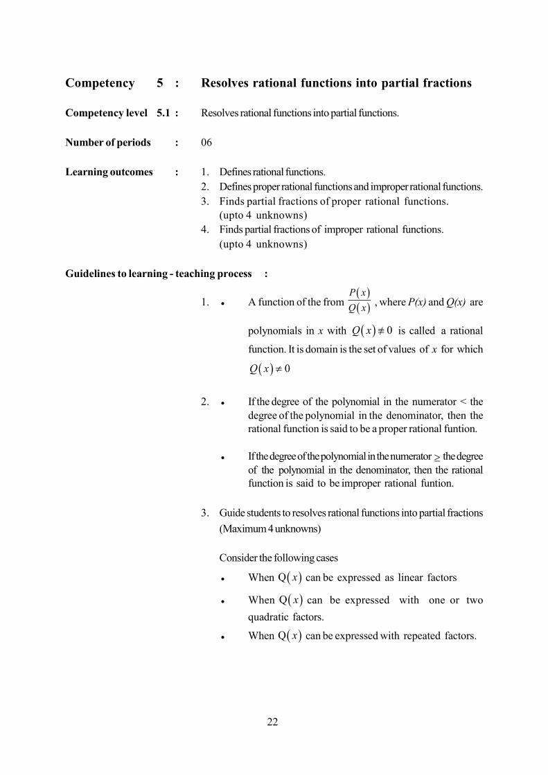
5.

2 4 0b ac

0a

2 4 0b ac

0a

2 4 0b ac

0a

2 4 0b ac

0a

.........................

x

y

................

.

y

y

x

y

.........................

x

x

y..............................

45

2 4 0

0

b ac

a

2 4 0

0

b ac

a

6. Describes zero of a quadratic function

Solves problems involving quadratic function

Competency level 3.2 : Interprets the roots of a quadratic equation.


Learning outcomes : 1. Explains the roots of a quadratic equation.

2. Finds the roots of a quardratic equation.

3. Expresses the sum and product of the roots of a quadratic

equation in terms of its coefficients.

4. Describes the nature of the roots of a quardatic equation.

5. Finds quadratic equations whose roots are symmetric

expressions of and .

6. Solves problems involving quadratic functions and quadratic

equations.

7. Transforms roots to other forms


1. State that when 0 a , a, b, c , 2 0ax bx c which

gives the zero points of the quadratic function is called the roots

of the quadratic equation.

.........................

y

x

.........................

y

x

46

2. Prove that a quardatic equation cannot have more than two

distinct roots.

Prove that a quardatic equation in a single variable can have only two

roots.

If roots are and then show that

2 4

2

b b ac

a

,

2 4

2

b b ac

a

3. If the roots of the quardatic equation 2 0ax bx c are

and then show that b

a

and

c

a .

4. Accordingly as 2 24 0, 4 0 andb ac b ac 2 4 0b ac , show

that the roots of the quardatic equation are real and distinct or real

and coincident or (imaginary) non real

Show the converse is also true.

Explain that the necessary and sufficient condition for the roots of

the quardatic equation to be real is2 4 0b ac

2 4b ac is called the discriminant of the equation

2 0ax bx c

Obtain the occassions, both roots are positive, both roots arenegative one is positive and other is negative and one root is zero,uisng the coefficient of the quardratic equation.

5. If the roots of the equation 2 0ax bx c are and obtain

equations of whose roots are symmetric expressions of and .

Eg: (i) 2 2 ,

(ii) 3 31, 1

(iii) ,

etc..

Discuss the condition of two quadratic equations to have acommon root.

6. Direct students to solve problems involving quadratic equations.

7. Use suitable transformation to find equation with symmetriccalexpressions..

47

Competency 12 : Solves problems involving inverse trigonometricfunctions.

Competency level 12.1 : Describes inverse trignometric functions.


Learning outcomes : 1. Defines inverse trignometric functions.

2. States the domain and the range of inverse trigonometric

functions.


1. Explain that if y = sin x, the value of x when y is given, is stated asx = sin-1 y and that x = sin-1 y is not a function. But it can be made afunction by limiting the domain of y = sin x.

2. Here the domain of sin x in generally limited to 2 2

x .

By interchanging x and y it can be denoted by y = sin-1 x where

1 1x 1sin

2 2

x .

Explain similarly that y = cos-1 x is definded such that10 cos x

Define, also, y = tan-1 x and explain that the values included in

the domain 2 2

x are its principle values.

y = sin-1 x; Domain [-1, 1], Range ,2 2

y = cos-1 x; Domain [-1, 1], Range 0,

y = tan-1 x;Domain , , Range ,2 2

48

Competency level 12.2 : Represents inverse function graphically.


Learning outcome : 1. Draws the graph of inverse trigonometric functions.

Guidelines to learning - teaching process :1. Draw the graphs of the following functions:

y = sin-1 x, y = cos-1 x, y = tan-1 x

States their domain and range.

Competency level 12.3 : Solves simple problems involving inverse trigonometric functions.


Learning outcomes : 1. Solves simple problems involving inverse trigonometric functions.

Guidelines to learning teaching process :1. Direct students to solve problems involving inverse trigonometric

functions.

49

Competency 11 : Applies sine rule and cosine rule to solvetrigonometric problems.

Competency level 11.2 : Applies sine rule and cosine rule.


Learning outcomes : 1. Proves sine rule.

2. Proves cosine rule.

3. Solves problems involving triangles using sine and cosine rules.


1. Proof of the sine rule, guide students to prove it for all three

triangles.

sin sin sin

a b c

A B C

2. Proof of the cosine rule, guide students to prove it for three

triangles.2 2 2 2 cosa b c bc A 2 2 2 2 cosb a c ac B 2 2 2 2 cosc a b ab C for all triangles

3. Direct students to solve problems including determination

of magnitude of angles or lengths of sides when sufficient

data is provided.

Guide students to solve problems involving the properties

of triangles.

50

Competency 13 : Determines the limit of a function.

Competency level 13.1 : 1. Explains the limit of a function.


Learning outcomes : 1. Explains the meaning of limit.

2. Distinguishes the cases where the limit of a function does not

exist.


1. When x discuss how the value of x, can approach a rational

number “a” without being equal to it.

2. Explains cases where limx a

f x

does not exist and distinguish

between the limit of a function at a point and the value of a function atthat point by examples. Explain graphically too.

Competency level 13.2 : Solves problems using the theorems on limits.


Learning outcome : 1. Expresses the theorems on limits.


1. Assume f and g to be functions for which a limit exist as x a ,where “a” is a real number.

1. let f x k when k is a constant, limx a

f x k

.

2. When k is a constant, lim limx a x a

k f x k f x

.

3. When k is a constant, f x k limx a

f x k

.

4. lim lim limx a x a x a

f x g x f x g x

.

5. lim lim limx a x a x a

f x g x f x g x

.

6. If lim 0,x a

g x

limlim

limx a

x a

x a

f xf x

g x g x

51

7. lim limnn

x a x af x f x

, n

8. lim limn nx a x a

f x f x

, n

When 0f x

9. When f is a polynomial function for all x

limx a

f x f a

.

10. If f x g x for all values of x except at x a in an

interval including a, then

lim limx a x a

f x g x

.

The proofs of the above theorems are not expected. Explain

their use in solving problems with examples.

Competency level 13.3 : Uses the limit: 1lim

n nn

x a

x ana

x a

to solve problems.


Learning outcomes : 1. Proves 1lim

n nn

x a

x ana

x a

where n is a rational number..

2. Solves problems involving above ersult.


1. Prove the theorem for positive integral values of n, and deduce it

for negative integral values of n.

Then prove that the theorem is true for any rational number n.

2. Direct students to solve suitable problems.

Competency level 13.4 : Uses the 0

sinlim 1x

x

x

to solve problems.


Learning outcomes : 1. States the sandwich theorem. (squeezes lemma)

2. Proves that 0

sinlim 1x

x

x

3. Solves the problems using the above result.

52


1. In an open interval containing a if for all values of x including or

excluding a, f x h x g x and

lim limx a x a

f x l g x

then limx a

h x l

.

The proof of this theorem is not necessary.

2. State that 0

sinlim 1x

x

x (x is measured in radians)

When x is measured in radians proves that

0

sinlim 1x

x

x by geometrical method.

Using the above results deduce that 0

sinlim 1x

x

x

3. Direct students to solve suitable problems.

Competency level 13.5 : Interprets one sided limits.


Learning outcomes : 1. Interprets one sided limits.

2. Finds one sided limits of a given function at a given real number.


1. Discuss lim ( ), lim ( )x a x a

f x f x

2. Convince the students that 0

1limx x

and 0

1limx x

using the

graph. Consider the domain as \ 0

3. Limits such as when , ( )x a f x and

, ( )x a f x are called infinite limits and are also known

as one side limits (left or right).recognize the cases

When x the limit of f(x) may be finite or infinite

53

Competency level 13.6 : Find limits at infinity and its application to find limit of rationalfunctions.


Learning outcomes : 1. Distinguishes the cases where a limit for f x either exist or

not as x approaches to infinity.

2. Explains horizontal asymptotes


1. In

limx

P x

Q x and

limx

P x

Q x ; 0Q x where P x and

Q x are polynomials and the degree of P x is n and that of

Q x is m.

Discuss seperately the cases when(i) n m (ii) n m (iii) n mwith suitable examples.State that these are known as limits at infinity.

2. In horizontal asymptote ocurse when

limx

f x l

(l is a finite value)

Competency level 13.7 : Interprets infinite limits.


Learning outcome : 1. Explains vertical asymptotes.


1. When vertical asymptote occures :

let ( )( )

( )

p xf x

q x .

Let a be a zero of q(x) and check whether

limx a

f x

and limx a

f x

Note : If there are many zeros for q(x), then there exist many

vertical asymptotes for f(x).

If there’s no zero for q(x),no vertical asymptote for f(x).

54

Competency level 13.8 : Interprets continuity at a point.


Learning outcome : 1. Explains continuity at a point by using examples.


1. Explain that, if

lim lim lim ( )x a x a x a

f x f x f x f a

Then the function is continous at x =a

55


Competency 2 : Uses systems of coplanar forces.

Competency level 2.4 : Explains the equilibrium of a particle under the action of three forces.


Learning outcomes : 1. Explains equilibrium of a particle under the action of three coplaner

forces.

2. States the conditions for equilibrium of a particle under the action

of three forces.

3. States the triangle law of forces, for equilibrium of three

coplanar forces.

4. States the converse of the triangle law of forces.

5. States Lami’s theorem for equilibrium of three coplanar forces

acting at a point.

6. Proves Lami’s Theorem.

7. Solves problems involving equilibrium of three coplanar forces

acting on a particle.


1. State that a particle acted upon by a system of coplanar forces is in

equilibrium, if the resultant of the system of forces is zero.

2. Show that the particle is in equilibrium under three coplanar forces

only if the resultant of any two forces is equal in magnitude and

opposite in direction to the third force.

3. Triangle law of forces

If three coplanar forces acting on a particle can be represented in

magnitude and direction by the three sides of a triangle taken in order,

then the three forces are in equilibrium.

Proves the theorem of triangle law of forces.

4. Converse of triangle law of forces

If three coplanar forces acting on a particle are in equilibrium then

they can be represented by three sides taken in order of a triangle

in magnitude and direction.

Prove the converse of the theorem of triangle law of forces.

Direct students to solve problems using the theorem of triangle of

forces and its converse.

56

5. Lami’s Theorem

If three coplanar forces acting at a point are in equilibrium then

magnitude of each force is directly proportional to the sine of the angle

between the other two forces.

It the particle is in equilibrium under three forces P, Q, R then

sin sin sin

P Q R

6. Prove Lami’s theorem.

7. Direct students to solve problems using

(i) Theorem of triangle law of forces and its converse.

(ii) Lami’s theorem.

Competency level 2.5 : Explains the resultant of coplanar forces acting on a rigid body.


Learning outcomes : 1. Describes a rigid body.

2. States the principle of transmission of forces.

3. Explains the translation and rotation of a force.

4. Defines the moment of a force about a point.

5. States the dimensions and units of moments.

6. Explains the physical meaning of moment.

7. Finds the magnitude of the moment about a point and its sense.

8. Represents the magnitude of the moment of a force about a point

geometrically.

9. Determines the algebraic sum of the moments of the forces abouta point in the plane of a coplanar system of forces.

10. Uses the general principle of moment of a system of forces.

R

QP

r

R

QP

r

57


1. Describe a rigid body as one in which the distance between anytwo points remains unchanged when it is subjected to externalforces of any magnitude.

2. Explain that a force acting on a rigid body can be considered asacting at any point on its line of action.

Also explain that the above phenomins is known as

transmission of forces.

3. Show that a linear motion as well as rotation can be created bya force.

4. Present the definition that the moment of the force about a point

is the product of the magnitude of the force and the perpendicular

distance to its line of action from the given point.

5. Show that dimension is 2 -2ML T and the unit is Nm

6. Build up the concept of moment as a measure of tendency to

rotate about a certain point as a result of an external force acting

on a rigid body. (For two dimensions only).

Make them to understand that what is measured by moment is a

turning effect about a line perpendicular to the plane determined

by that point and the line of action of the force

7. Demonstrate that the sense of the moment can be considered as

clockwise or anticlockwise. Explain that according to sign

convention an anticlockwise moment is considered positive and

a clockwise moment is considered negative.

Moment of 1F about O = 1 1F d .

Moment of 2F about O = 2 2F d

O = 2 2-F d

>

F1

d1

>F

2

d2

58

8. Explain that the magnitude of the moment of a force F denoted in

magnitude, direction and position by AB

about a point O is twice

the area of the triangle OAB.

9. Direct students to solve problems of finding the algebraic sum of the

moments of a system of coplanar forces about a point in the plane.

10. State that the algebraic sum of moments of a system of coplanar forces

about a point in the plane is equal to the moment of the resultant of the

system about the same point. (Proof is not expected). Explain using

suitable examples.

Guide students to solve problems involving moments

Competency level 2.6 : Explains the effect of two parallel coplanar forces acting on a rigidbody.


Learning outcomes : 1. Uses the resultant of two non parallel forces acting on a rigid

body.

2. Uses the resultant of two parallel forces acting on a rigid body.

3. States the conditions for the equilibrium of two forces acting on a

rigid body.

4. Describes a couple.

5. Describes the sense of a couple

6. Calculates magnitude and moment of a couple.

7. States that the moment of a couple is independent of the point

about which the moment of the forces is taken.

8. States the conditions for two coplanar couples to be equivalent.

9. States the conditions for two coplanar couples to balance each

other.

10. Combines coplanar couples


1. When the two forces are no parallel

As the two forces meet at a point show that their resultant can be

determined by applying the parallelogram law of forces.

2. When the two forces are parallel

Introduce that forces acting on lines parallel to each other are

known as parallel forces.

59

When two parallel forces are acting in the same direction they are

said to be like forces, while those acting in opposite directions

are said to be unlike forces.

Explain that the parallelogram law of forces cannot be used to

find the resultant of two parallel forces.

If the two forces are P and Q and their resultant is R, and if the

lines of action of P, Q and R intersect a certain straight line at A,

B and C respectively.

if P and Q are like, R = P + Q

P > Q P < Q

P AC Q BC P AC Q BC

If P and Q are unlike

if (P>Q), if (P<Q)

Show that for two forces acting on a rigid body are in

equilibrium, the two forces should be collinear, equal in

magnitude and opposite in direction.

3. Introduce a couple as a pair of parallel unlike (opposite) forces of

equal magnitude. In this case, show that the vector sum of the two

forces is zero, the algebraic sum of the moments of the two forces

about any point is not zero. Therefore there is no translation, but only

a rotation of the body.

P Q

A C B

R R Q

A BC

P

A C

Q

B

R = P - QP.AC=Q(BC)

R P

A C

Q

B

R = Q - PP(AC)= Q(BC)

R

60

4. Show that the moment of a couple about any point in the plane of the

couple is the product of the magnitude of one of the forces forming the

couple and the perpendicular distance between the lines of action of

the two forces.

5. Mention that according to sign convention the anticlockwise (left

handed) moments are considered as positive whereas clockwise (right

handed) moments are considered to be negative.

6.

Moment of the couple = F d Moment of the couple = F d

= -F d = -F d

7.

The moment of two forces about

O = 1 2 1 2Fd Fd F d d O = 1 2 1 2Fd Fd F d d

= F d = F dShow that the same result will be obtained by taking moments about

any point in the plane of the couple.

8. As two coplanar couples with moments of equal magnitude and same

sense produce same rotation, they are equivalent.

9. As the resulting rotation when two coplanar couples of equal

magnitude but of opposite sense, produce zero rotation, two such

couples are said to balance each other.

10. Explain that the algebraic sum of moment should be taken in finding

the moment of the combination of two or more coplanar couples.

FdF

FdF

d

F F

d 1

Od 2

d

F F

d 2

O

d 1

61

Competency level 2.7 : Analysis of a system of coplanar forces acting on a rigid body.


Learning outcomes : 1. Reduces a couple and a single force acting in its plane into a

single force.

2. Shows that a force acting at a point is equivalent to the combination

of an equal force acting at another point together with a couple.

3. Reduces a system of coplanar forces to a single force acting at O

together with couple of moment G.

4. Finds magnitude, direction and l ine of action of a system of

coplaner forces.

5. Reduces a system of coplanar forces to a single force acting at

a given point in that plane.

6. (i) Expresses reduction of a system of coplanar forces to a

single force when it reduces to a single force.

(ii) Expresses reduction of a system of forces to a couple.

(iii) Expresses conditions necessary for equilibrium.

7. Solves problems involving rigid bodies under the action of coplaner

forces.


1.

G p R

Gp

R

R

R

-R

B

A

p

A A B B

R RR

R

R

GG

62

Show that a couple of moment G and a single force R acting in itsplane is equivalent to a force equal and parallel to a force R acting at

a distane G

R from the point of action of it.

2. Show that the force F acting at P is equivalent to the combination of a

force F acting at a point Q and a couple of moment G F d , where

d distance between the lines of action of the two forces F.

3. Show how a system of coplanar force is reduced to a single force R actingat origin O and a couple of moment G.

Consider the system of coplanar forces F, acting at Pr (X

r, Y

r).

where r = 1, 2, ......, n

1

R Fn

rr

= r r1

X Yn

r

i j

= r r1 1

X Yn n

r r

i j

= X Yi j

Where X =1

Xn

rr and

Y =1

Yn

rr .

O

Yr

XrP

r(X

r, Y

r)

x

y

Fd

PQ

F

F

G

63

4. Magnitude of R

2 2R X Y

R makes an angle θ with the X - axis

θ = 1 Y

tanX

G = 1

Y Xn

r r r rr

x y

anti clockwise.

Show that the equation of the line of action is

G - Y X 0x y .

5. Show how it can be reduced to a single force /R acting at the point

P(x, y) in the plane and a couple /G

6. Obtain that/R = R and/G = G Y Xx y

Present the following necessary and sufficient conditions for two

coplanar systems of forces to be equivalent.

That when each system of forces is resolved seperately along two

axes Ox and Oy perpendicular to each other selected in the plane of

the two systems of forces each algebraic sum of components of one

system of forces is equal to the corresponding algebraic sum of the

other system of forces.

/ /X X, Y Y , where X and Y are the algebraic sums of one

system of forces along Ox and Oy and / /X , Y are the algebraic sums

of the other system of forces along the same axes.

If the algebraic sum of the moments of the two systems of forces

about any point (h, k) in the plane, are

/1G and /

2G , /1G = /

2G

64

7. When a system of coplanar forces is reduced to a single force

R X Yi j acting at the origin O and couple of moment G,,

discuss cases to reduce a system a of coplaner forces to a couple,

(i) R 0 (i.e. at least one of X or Y should not be zero). Show

that when G = 0 it is reduced to a single force through origin and

when 0G it is reduced to a single force through another point.

(ii) Show that R 0 (i.e., X = 0 and Y = 0) and G 0 (system reduced to ) reduces to a couple.

(iii) If R 0 (i.e., X = 0 and Y = 0) and G = 0.

Show that the systems of forces are in equilibruim.

Give suitable examples for each condition.

65

Competency 3 : Applies the Newtonian model to describe theinstantaneous of motion in a plane

Competency level 3.1 : Uses graphs to solve problems involving motion in a straight line.


Learning outcomes : 1. Defines “distance and speed”

2. States diamention and units of distance and speed.

3. Defines average speed.

4. Defines instantaneous speed.

5. Defines uniform speed.

6. States dimensions and standard units of speed.

7. States that distance and speed are scalar quantities.

8. Defines position coordinates of a particle undergoing rectilinear

motion. (motion in a straight line)

9. Defines Displacement.

10. States the dimension and standard units of displacement.

11. Defines average velocity.

12. Defines instantaneous velocity.

13. Defines uniform velocity.

14. Expresses dimension and units of velocity.

15. Draws the displacement -time graph.

16. Draws velocity - time graph.

17. Finds the average velocity between two positions using the dis

placement time graph.

18. Determines the instantaneous velocity (between two positions)

using the displacement time graph.

19. Defines accelaration.

20. States the dimension and unit of acceleration.

21. Defines average acceleration.

22. Defines instantaneous acceleration.

23. Defines uniform acceleration.

24. Defines retardation.

25. Draws the velocity time graph.

26. Finds average accelaration using the velocity time graph.

27. Finds the acceleration at a given instant using velocity - time graph.

28. Finds displacement using velocity time graph.

29. Draws velocity time graphs for different types of motion.

30. Solves problems using displacement time and velocity-time graph.

66


1. Distance: When a variable point P moves from a point A to a

point B present the length measured along the path form A to B

as the distance travelled by the point.

Speed : Speed is defined as the rate of change of distance with

respect to time.

State dimensions and standard units of distance.

2. Dimensions of distance : L Standard unit is meter (m).

Introduce and other units of distance such as mm, cm, km.

3. If the total distance travelled from A to B is s, and the time taken

is t then define that s

t as the average speed during the time

interval t.

4. The speed of a moving particle at a given instant of time is defined

as the instantaneous speed at that time.

5. If the instantaneous speed of a particle over a certain time interval

remains constant, define that speed as a uniform speed.

6. Dimension of speed 1LT ;

Standard unit is 1ms .

Introduce other units of speed such as 1kmh .

7. Distance is a quantity with a magnitude measured with some unit.

Time is also same. Since they do not possess a direction

demonstrate that distance and speed are scalar quantities.

8. The position coordinate of a point P moving along a line ‘l’ is

denoted by ‘x’, and defined as OPx depending whether its

position is on the right or left of the point O.

Explain that x is a function of time t.

O Px

67

9. Define displacement as the change in the position coordinate during

a given time interval.

If the position coordinate of the particle P at times 1t and 2t are

1x and 2x respectively, show that the displacement s of the

particle during the time interval 1 2, t t is defined as 2 1s x x .

Explain that the displacement is a vector quantity.Show also that accordingly as s > 0 or s < 0 its direction istaken as or .

10. Dimension L; Standard unit is m (meter)

Explain other units too in terms of the standard units ,cm km

11. During the time interval 1 2, t t let the displacement be

2 1s x x . Average velocity during that time interval is de

fined as 2 1

2 1

x x

t t

and also show that average velocity can be

positive or negative.Average velocity too is a vector quantity.

The average velocity of a particle during a small interval ,t t h

is given by t h tx xh

12. Average velocity of the particle when 0h

0lim t h t

n

x x dsVh dr

13. Introduce this velocity as the instantaneous velocity of the

particle at time ‘t’. Show that ds

vdt

and explain that velocity is

also a function of time.

If the displacement ‘s’ is measured from a fixed point

O then show that v can also be written as ds

vdt

,

velocity is the rate of change of displacement with respect to time.

By sign convention, accordingly as 0v or 0v , its direction

is taken as or .

68

14. Velocity: Velocity is defined as the rate of change of displacement with respect to time.

15. Dimension of velocity v is 1LT and standard unit is 1ms .

Also explain other units in terms of the standard unit

( 1 1,cms kmh )

16. Using suitable examples to explain that how displacement time

graph is drawn.

17. If 1s and 2s are the displacements corresponding to the times 1t

and 2t show that the average velocity 2 1

2 1

s s

t t

can be obtained by

the gradient of the line 1 2P P . Here 1P and 2P are points on the

displacement - time curve corresponding to times 1t and 2t

respectively.

18. Show that the gradient of the tangent drawn to the displacement

time graph, at a particular point gives the instantaneous velocity

at that moment.

Obtain the relation instantaneous velocity = ds

dt

= gradient

19. Acceleration: Define acceleration of the velocity - time curveat time t of the tangent as the rate of change of velocity withrespect to time.Since velocity is a vector, acceleration also is a vector.

20. Express that the dimension of acceleration is 2LT and the

Standard unit is, meters per meter per second squared 2ms.

Mention other units of acceleration such as 2 2,cms kmh

21. If the velocities of a particle are 1v and 2v at times 1t and 2t

respectively, then define the average acceleration of the particle

during the time interval 1 2, t t as 2 1

2 1

v v

t t

.

Show that average acceration 0 accordingly as 2V 1V

69

22. The average acceleration during a small time interval ,t t h is

t h tv v

h

.

As 0h , the limit of the average acceleration

0lim t h t

h

v va

h

Introduce a as the instantaneous acceleration at time t.

Show that dv

adt

. This is known as the acceleration of the

particle at time t.Explain that acceleration is a function of time.Emphasize the fact that acceleration is the rate of change ofvelocity with respect to time.

23. If the acceleration is constant in a certain time interval, define that

motion as a motion with uniform acceleration.

24. State that when the acceleration is negative it is called a

retardation.

25. Provide an understanding of drawing velocity time graphs using

suitable examples.

26. If the velocities corresponding to times 1t and 2t are 1v and 2v

respectively, then show that the average acceleration during the

time interval 2 11 2

2 1

, isv v

t tt t

. It can be obtained as the

gradient of the line 1 2P P . Here 1P and 2P are two points

corresponding to times 1t and 2t in the velocity time curve.

27. Show that the gradient of the tangent drawn at a given point to

the velocity time graph gives the instantaneous acceleration at the

time represented by the point. Deduce that instantaneous

acceleration

dva

dt (gradient). Show also that

dva v

ds .

70

28. Explain that displacement during a certain time - interval is given

by the area between the graph and the time axis. (An area below

the time axis is assigned a negative sign).

29. Direct students to draw velocity time graphs for

1. Position of rest - zero velocity.

2. Uniform velocity.

3. Uniform acceleration.

4. Uniform retardation.

5. A combinations of such motions.

30. Direct students to solve problems related to rectilinear motion

with uniform acceleration.

Competency level 3.2 : Uses kinematic equation to solve problems involving motion in a stright

line with constant acceleration.


Learning outcomes : 1. Derives kinematic equations for a particle moving with uniform

acceleration.

2. Derives kinematic equations using velocity - time graph.

3. Uses kinematic equations for vertical motion under gravity.

4. Uses kinematic equations to solve problems.

5. Uses velocity - time and displacement - time graphs to solve

problems.


1. Introduce the standard symbols for

initial velocity - u ; final velocity - v

acceleration - a ; time - t and

displacement - s and derive the kinamatic equations.

v u at

1

2s u v t

21

2s ut at

2 2 2 v u a s

71

2. Guide students to derive kinematic equations using velocity-timegraph.

3. Show that in this case the acceleration should be replaced by g,(the acceleration due to gravity) which is a constant.Show that g is taken approximately as 10ms-2 and remind assumptions.

4. Explain using suitable examples.

Competency level 3.3 : Investigates relative motion between bodies moving in a straight line

with constant acceleration.


Learning outcomes : 1. Describes the concept of frame of reference for two dimensional

motion.

2. Describes the motion of one body relative to an other when two

bodies are moving in a straight line.

3. States the principle of relative displacement for two bodies mov

ing along straight line.

4. States the principle of relative velocity for two bodies moving

along a straight line.

5. States the principle of relative acceleration for two bodies

moving along a straight line.

6. Uses kinematic equations and graphs related to motion for two

bodies moving along the same straight line with constant relative

acceleration.


1. Introduce that a particle moving (on a straight line) and an axisfixed rigidly to the particle so that it lies along the line constitute aframe of reference.

2. Explain with examples.

3. If the displacement of particles P and Q relative to the frame of

reference O on a straight line are P,Os and Q,Os respectively

express the displacement of Q relative to P as Q,P Q,O O,Ps s s .

Show that O,P P,Os s .

72

4. Obtain Q,P Q,O O,Pv v v by differentiating the displacement

equation with respect to time.

5. Obtain the relation Q,P Q,O O,Pa a a by differentiating the

velocity equation with respect to time.

Find relative displacement, relative velocity and relative

aceleration for two particles moving along two parallel paths.

6. Explain using suitable examples.

Consider only cases where the distance between the parallel paths

is negligible.

7. Guide students to solves related problems.

73

Third Term

74

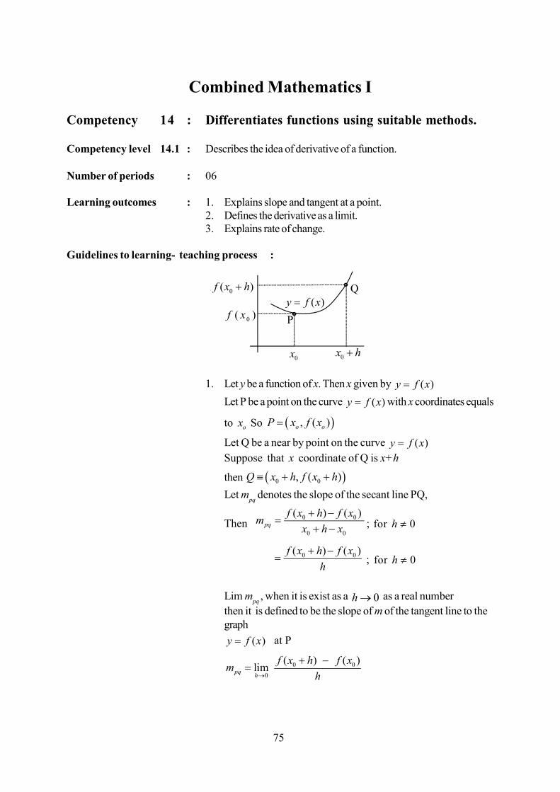
75


Competency 14 : Differentiates functions using suitable methods.

Competency level 14.1 : Describes the idea of derivative of a function.


Learning outcomes : 1. Explains slope and tangent at a point.2. Defines the derivative as a limit.3. Explains rate of change.

Guidelines to learning- teaching process :

1. Let y be a function of x. Then x given by ( )y f x

Let P be a point on the curve ( )y f x with x coordinates equals

to ox So , ( )o oP x f x

Let Q be a near by point on the curve ( )y f x

Suppose that x coordinate of Q is x+h

then 0 0, ( )Q x h f x h

Let mpq

denotes the slope of the secant line PQ,

Then 0 0

0 0

( ) ( )pq

f x h f xm

x h x

; for 0h

0 0( ) ( )f x h f x

h

; for 0h

Lim mpq

, when it is exist as a 0h as a real number

then it is defined to be the slope of m of the tangent line to thegraph

( )y f x at P

0 0

0

( ) ( )limpqh

f x h f xm

h

0( )f x

Q

0x 0x h

( )y f x0( )f x h

P

76

equation of the tangent line at P to the curve ( )y f x with slope

m is, 0 0( ) ( )y f x m x x

2. The limit 0 0

0limh

f x h f x

h

which was used to define the

slope of the tangent line is given a name and a notation. Since itoccurs in many other situations it is called derivative of f(x), at

x a , and it is denoted by 0( )f x provided the limit exists (as a

real number) ( )f x is differentiable at 0x x .

Using suitable examples , explain that the derivative of f(x) does

not exist at 0x x . in the instances given below..

(i) When f is not defined in an open interval including 0x x

(ii) When 0 0

0limh

f x h f x

h

is not finite

(iii) When 0 0

0limh

f x h f x

h

is not defined

The function f whose domain consists of all values of x at which

the derivative exists is called the derivative function of f(x)

so ( ) ( ) ( )f x f x and

( ) ( )( ) lim

h o

x h f xf x

h

3. Let y be a function of x given by ( )y f x . Take any x and

consider an increment of x is consider the change in x in the

closed interval with x and x x as its end points.

0( )f x

0x

P p

( , )x y

( )f x

( )f x x

x x x x<

<

y

77

x is the change in x values the corresponding change in y

values denoted by y is equal to ( ) ( )f x x f x

Therefore the average rate of change in y with respect to x in the

closed interval with x and x x as its end points is y

x

this ( ) ( )y f x x f x

x x

Emphasize that x is a symbol and not a product of and x

The Instantaneous rate of change of y with respect to x is de

fined to be 0 0

( ) ( )lim lim

x x

y f x x f x

x x

provided the limit exist as real number

Note that 0lim ( )

x

yf x

x

0lim

x

y

x

is also denoted by dy

dx

Hence ( )f x is the same as dy

dx

Competency level 14.2 : Determines the derivatives from the first principles.


Learning outcomes : 1. Finds derivatives from the first principles.


1. When n is a rational number, showing the method of determining

the derivative of nx and the derivatives of basic trigonometric

functions from first principles. Present the proofs of the followingresults.

1 n ndx n x

dx 2cot cos ec

dx x

dx

sin cosd

x xdx

sec sec tand

x x xdx

cos sind

x xdx

cos ec cos ec cotd

x x xdx

2tan secd

x xdx

78

Competency level 14.3 : States and uses the theorems and rules of the differantiation.


Learning outcomes : 1. States the basic rules of derivatives.

2. Solves problems using basic rules of derivatives.


1. Prove that, When k is a constant

(i) When k is a constant and f x k then 0f x .

(ii) If f x kg x then f x kg x .

(iii) If f x g x h x then

/ /f x g x h x

Direct students to solve problems using 1

n

nd x

nxdx

and the above theorems after explaining suitable examples.

2. (i) Product rule

d

f x g xdx

= d d

f x g x g x f xdx dx

(ii) Quotient rule

f xd

dx g x

=

2

d dg x f x f x g x

dx dx

g x

,

Where 0g x

(iii) Chain rule

If y is a function of u and u is a function of x then

dy dy du

dx du dx

Chain Rule and its extension proofs are not required of theabove results.

Solves problems using above results.

79

Competency level 14.4 : Differentiates inverse trigonometric fucntions.


Learning outcomes : 1. Finds the derivatives of inverse trigonometric functions.

2. Solves problems using the derivatives of inverse trigonomatric

functions.


1. Deduces that

(i) 1

2

1sin , 1 1

1

dx x

dx x

(ii) 1

2

1cos , 1 1

1

dx x

dx x

(iii) 1

2

1tan ,

1

dx x

dx x

2. Differentiates various functions using the above formulae.

Competency Level 14.5 : Describes natural exponential function and find its derivative.


Learning outcomes : 1. Defines the exponential function (ex)

2. Express domain and range of the exponential function.

3. State that e is an irrational number.

4. Describes the properties of the ex.

5. Writes the estimate of the value of e

6. Writes the derivative of the exponential function and uses it tosolve problems.

7. Sketches the graph of e-x

Guidelines to learning - teaching process :1. States that the sum of the infinite series

2

1 ........ ........1! 2! !

nx x x

n is donated by xe

xe is called the natural exponential function.

2. State that the domain of the natural exponential function in and

the range is (0, )

80

3. by taking 1x we get

1 1 1 11 ....... .......

1! 2! !e e

n

State that e is an irrational number and that e 2.718

4. State that

(i) 0 1e

(ii) 1 2 1 2x x x xe e e

(iii)1

1 2

2

xx x

x

ee

e

(iv) for rational values of r, ( )x r rxe e

(v) lim x

xe

(vi) lim 0x

xe

5. 1 1 1 1

1 1 ... ... 2.7181 2 3

f en

Stress that e is a positive irrational number.

6. States that x xd

e edx

Solves problems involving natural exponential functions.

7. Guide students to draw the graph of xy e

At this stage only the shape of the graph is needed

Competency level 14.6 : Describes natural logarithmic functions.


Learning outcomes : 1. Defines the natural logarithmic functions.

2. Expresses the domain and range of the logarithmic functions.

3. Expresses the properties of ln x

4. The graph of y = ln x

5. Defines the function ax for a > 0

6. Expresses the domain and range of the function ax

7. Solves problems involving logarithmic functions.

8. Deduces the derviative of ln x

9. Deduces the derviative of ax

10. Solves problems using the derviative of ln x and ax

81


1. Explain that ln x defined by . yy ln x x e ln x is called the

natural logarithimis function of ex

2. If ( ) ,g x ln x then the domain of g is (0, ) and the range is

3. (i) ln x is edfined only for 0x

(ii) ( ) ,xln e x for x

(iii) ln xe x for 0x

(iv) ( ) ln x y ln x ln y for 0x and 0y

(v) x

ln ln x ln yy

for 0x and 0y

(vi) ( ) ; 0bln x bln x x

4. Sketch the graph of ,y ln x using the inverse property..

The graph of ,y ln x is the mirror image of xy e on y x

5. The function xa is defined lnx x aa e

6. If ( ) xh x a , then the domain of h and the range of (0, )h

7. Solves problems involving natural logarithmic function.

8. Deduce that

(ln ) 1, 0

d xx

dx x

9. Deduce that ( )

( )x

xd aln a a

dx

10. Solves problems using the derivative of ax

Competency level 14.7 : Differentiate implicits functions and parametric functions.


Learning outcomes : 1. Define implicit functions.

2. Finds the derivatives of implicite functions.3. Differentiates parametric functions.4. Writes down the eqautions of the targent and normal at a given

point to a curve.

82


1. A function defined by

( )y f x , which statisfies an equation of the ( , ) 0F x y is called an

impliciat function.

Explain this using 2 2 1 0x y

2. To obtain the derivative of an implicit function ( )y f x defined by an

equation ( , ) 0f x y , not necessary (sometimes not possible) it is

to solve ( , ) 0f x y , explicity for y in terms of x and then get the

derivative. We instead differentiate the both sides of ( , ) 0f x y with

the chain rule. Explain using examples

A curve C is defined by the parametric equation ( )x f t and

( )y f t where t is a parameter..

Then the derivative dy

dxcan be obtained from

dy

dy dt

dxdx

dt

at points for which 0dx

dt .

Show also that

2

2

d dy

d y dt dt

dxdx

dt

at points for which 0dx

dt .

Explains using examples

3. Differentiation involving implicit functions and parametric forms for

the parabola 2 4 ,y ax elipse 2 2

2 21

x y

a b and the hyperabola

2 2

2 21

x y

a b > 2xy c

83

2 4y ax : 2 , 2x at y at

2 2

2 21

x y

a b : cos , sinx a y b

2 2

2 21

x y

a b : sec , tanx a y b

2xy c : , c

x ct yt

4. Obtains equations of tangent and normals at points on curves

defined parametrically, including the above curves.

Show how to sketch the above mentioned curves and explains

their elementary properties.

Competency level 14.8 : Obtains derivatives of higher order.


Learning outcomes : 1. Finds derivatives of higher order.

2. Differentiats functions of various types.

3. Finds relationship among various order of derivatives.


1. If y is a function of x , then thn order derivative of y is obtained by

differentiating y n times with respect to x. This is denoted by

( ) ( )( )n

n n

n

d yor f x or y

dx

2. Explain using examples

3. Guide students to solves problems involving higher order derivatives,

84

Competency 15 : Analysies the behaviour of a function usingderivatives

Competency level 15.1 : Investigates the turning points using derivatives.


Learning outcome : 1. Defines stationary points of a given function.

2. Describes increasing or decreasing function.

3. Describes local (relative) maximum and local minimum.

4. Employs the first derivative test to find the maximum and

minimum points of a function.

5. States that there exists critical points, which are neither a local

maximum nor a local minimum.

6. Introduces points of inflection.

7. Uses the second order derivative to test whether a turning

point of a given function is a local maximum or a local

minimum.


1. A point at which the derivative of a function is zero is defined as a

stationary point. So, ( )f x has a stationary point when x c

provided that ( ) 0f c explains with suitable examples.

2. Explain that a function ( )f x increasing on an interval I, if

1 2( ) ( )f x f x whenever 1 2, ,x x I with 1 2x x

Explain that it ( ) 0f x for x I , then ( )f x is strictly

increasing on I.

Explain that a function ( )f x is decreasing on an interval

I it 1 2( ) ( )f x f x whenever 1 2, ,x x I with 1 2x x

Explain that it ( ) 0f x for ,x I then ( )f x is strictly

decreasing on I.

85

3. State that if there exists 0 such that ( ) ( )f x f c for

all ( , ),x c c then ( )f x is said to have a

maximum at x a

State that if there exists 0 such that ( ) ( )f x f c for

all ( , ),x c c then ( )f x is said to have a

minimum at x a

4. Describes the first derivative test for local maximum nor localminimum.

5. States that there exists stationary points which are neighterlocal maximum nor local minimum.

Discuss with examples in which ( ) 0f c but the point

which neither local maximum nor local minimum

6. Introduce the point of inflection.

7. If ( ) 0 ( ) 0f a and f a then there is a local

maximum at x a

If ( ) 0 ( ) 0f a and f a then there is a local minimum

at x a

Guide to solves problems involving maxima and minima.

Competency level 15.2 : Investigates the concavity


Learning outcomes : 1. Uses second derivative test to find concavity.


1. State that it ( ) 0f x for ( , )x a b then the graph of f is

concave upwords, and if f (x) < 0 for ( , )x a b then the graph

of f is concave down words.

Explain that a point of inflection is a point at which concavity

changes

Give examples to show that the derivative need not be zero at the

point of intection.

86

Competency level 15.3 : Sketches curves.


Learning outcome : 1. Sketches the graph of a function.


1. Direct students to draw graphs of function using the above

principles.

Examples involving horizontal and vertical asymptotes are also

included.

Competency level 15.4 : Applies derivatives for practical situation


Learning outcome : 1. Uses derivatives to solve real world problems.


1. Direct students to solve problems involving maximum and

minimum in real world activities.

87


Competency 3 : Applies the Newtonian model to describe theinstantaneous of motion in a plane

Competency level 3.7 : Interprets the motion of a projectile in a vertical plane.


Learning outcomes : 1. Introduces projectiles.

2. Describes the terms “velocity of projection” and “ angle of

projection”.

3. State that the motion of a projectile can be considered as two

motions separately in the horizontal and vertical directions.

4. Applies the kinematic equations to interpret motion of a projectile.

5. Calculates the components of velacity of a projectile in a given time.

6. Finds the components of displacement of a projectile in a given time.

7. Calculates the maximum height of a projectile.

8. Calculates the time taken to reach the maximum height of a

projectile.

9. Calculates the horizontal range of a projectile and its maximum.

10. States that in general there are two angles of projection for

the same horizontal range for a given velocity of projection.

11. Finds the maximum horizontal range for a given speed.

12. For a given speed of projection finds the angle of projection

giving the maximum horizontal range.

13. Derives Cartesian equations of the path of a projectile.

14. Finds the time of flight.

15. Finds the angles of projection to pass through a given point.

Guidelines to learning- teaching process :

1. Introduce a projectile as a particle or a body moving freely undergravity.

2. When a particle or a body is projected with a velocity u inclinedat an angle to the horizontal introduce that u is the velocity ofprojection and is the angle of projection.

3. Explain that the velocity component is constant for the horizontalmotion and the acceleration, (which is due to gravity), is constant for the vertical motion. In fact, accelaration a = g directedvertically down wards.

88

4. Show that the following equations can be used with a g ,

Horizontally : coss ut s u t

Vertically : ( sin )v u at v u t gt

2 21 1: ( sin )

2 2s ut at y u t gt

2 2 2 2 22 : sin 2v u a s v u gy

s, u, v, a, t have usual meanings.

5.

Derive that the horizontal and vertical components of velocity at

a time t, are cosxV u t , sinyV u gt

6. Derive that the components of displacement at time t as x and y,state that these are parametric equations of the path of theprojectile where “t” is the parameter.

7. Show that if H is the maximum height then

2 2sinH

2

u

g

>

>

>

>

t = t t = 0

u

y

x

V sinu gty

V cosux

>P(x,y)

>

>

>

>

>u

A

OB

x

y

O

H

Vy

89

>

>

u

u

><

2

y

x

8. Show that if T is the time taken to reach the maximum height, then

0 BT T ,

sinT

u

g

9. If R is the horizontal range through the point of projection derive

the expression for horizontal range R,

22 sin cosuR

g

10. Show that there are two angles of projection giving the samevalue for a given projection speed.

for a given u 2sin 2

gR

u

sin 2 sin 2

2 2 180 2

90

or

or

sin 2 sin 2

2sin cos 2sin cos

2

or

sin sin

sin cos

or

90

R which is obtained when and 2

are substituted

in the the expression for the same horizontal range

22R cos sin

u

g

Time of flight 2 sin

2u

Tg

2 sin( cos ) 2

uR u T

g

11. As

2 2sin 2R

u u

g g

deduce that

2

maxRu

g , for given u.

12. Derive that the angle of projection giving the maximum horizontal

range is 4

.

13. Derive the equation 2 2

2

sectan

2

gxy x

u

by eliminating

t from the equation obtained earlier for x and y

when 2

compare this with the quadratic function

2y ax bx , which represents a parabola through the point of

projection.

Remind that 2

gives vertical motion under gravity..

14. If T is the time taken to return to the level of the point ofprojection, then show that

2 sin

T 2Tu

g

.

15. Guide to find the angle of projection to passing through a pointfor a given velocity.

91

Competency 2 : Uses systems of coplanar forces.

Competency level 2.8 : Explains the equibirum of three coplanar forces acting on a rigid body

as a particular case.


Learning out comes : 1. States conditions for equilibrium of three coplanar forces

acting on a rigid body.

2. Finds unknowns when a rigid body is in equilibrium using,

² Triangle law of forces.

² Lamis theorem, cotangent rule.

² Geometrical properties.

² Resolving in to directions perpendicular to each other.


1. If three coplanar forces acting on a rigid body are in equilibrium

then their lines of action passing through the same point or

else they are parallel.

Explain that this is a necessary condition only.

2. ² State the triangle law of forces and its converse.

(This has been presented under the equilibrium of a

particle.)

Using the triangle of forces, ABC, show that,

P Q R

AB BC CA

Use this result in solving problems.

Corresponding triangle of

forces, ( ABC ).

Three forces P, Q, R

acting at O are in

equilibrium O

Q

R

PO

A >

>>R

PB

Q

C

92

² Lami’s theorem (Presented under equilibrium of a particle)

Explain that this theorem can also be applied in solving problems

involving equilibrium of three coplanar non parallel forces whose

lines of action are concurrent.

² Cot rule

Type 1: cot A cot Bn m = cot θm n

Type 2: cot cotm n = cot θm n

Show that, using examples the above results can be used in

solving problems.

² In solving problems make use of the geometrical properties ofthe diagram as far as possible.

² Consider the equilibrium which is three forces are parallel. In that

condition magnitude of resultant that of two forces is equal to the

third force opposite in direction and their lines of action are same.

² State that the algebraic sums of resolutes along two

perpendicular directions seperately are zero.

Competency level 2.9 : Investigates the effect of friction


Learning out comes : 1. Describes “Friction” and “Frictional force”.

2. Distinguishes between smooth and rough surfaces.

3. States the advantages and disadvantages of friction.

4. Whites the definion of “Limiting frictional force”.

5. State laws of friction.

6. Defines angles of friction and coefficient of limiting friction.

7. Expresses the conditions for equilibrium.

8. Solves problems related to equlibrium of a particle or a rigid body,

under the action of forces including frictional force.

A B

C

m n

α β

θ

93


1. ² Introduce frictional force as a force acting along the tan

gential plane that prevents or tends to prevent relative

motion between two bodies in contact. The property that

produces this force is called friction.

² State that as the applied force is gradually increased the

frictional force too increases until the equilibrium ceases

to exist

2. From the surfaces incontact, introduce that the surfaces without africtional force as smooth surfaces and surfaces with a frictional

force as rough surfaces.

3. Discuss the advantages and disadvantages of friction using suit

able esamples.

4. Introduce “Limiting frictional force” as the masimum frictional forcebetween two surfaces at the instant when relative motion between

the two surfaces in contact is about to commence.

5. ² When two bodies in contact under go motion relative to

each other the frictional force exerted by one body onthe other is opposite to the direction in which the bodymoves or tends to move relative to the other.

² When in limiting equilibrium the frictional force is just sufficient to prevent relative motion.

² The ratio of the limiting frictional force to the normal

reaction at the point of contact is a constant, called the

coefficient of limiting friction and depends only on the

material the surface of the bodies are made of.

² As long as the normal reaction remains unchanged, the

limiting frictional force does not depend on the area of

contact or the shape of the two surfaces.

² When the motion sets in the limiting frictional force

decreases slightly.

² When there is relative motion between the surfaces, the

ratio of the frictional force and the normal reactions is

slightly less than the coefficient of limiting friction.

94

6. ² Define the coefficient of limiting friction between any twogiven surface as the ratio of the limiting frictional force to

the normal reaction. If Fl is the limiting frictional force and

R is the normal reaction then F

Rl

l is called coefficient

of limiting friction. This is also called the coefficient of

static friction

² Introduce the angle of friction as the angle made by the resultant reaction with the normal reaction whenthe equilibrium is limiting.

² If the angle of friction is ; deduce the result l = tan .

tanF

R

7. ² States the conditions for equlirium

² Express that the frictional force F between two

surfaces in contact at any time is given by F l .

(equality occuring at limiting equilibrium) and F Rl .

8. Direct students to solve problems involving friction.

O

R

>

>>

>

R = F

R1

95

Competency level 3.4 : Explain the motion of partcle on a plane


Learning out comes : 1. Finds relation between the Cartesion coordinates and the polar

coordinates of a particle moving on a plane

2. Finds the velocity and accelaration when the position vector is

given as a function at time.

1.

² If A is a fixed point, OA is a fixed line and P is a variable

point such that OP = r and AOB then state that the

polar coordinates of the point P is defined as ,r .

Where r O , and the angle is measured anti clock

wise is taken to be positive. Show that a point can also bedenoted uniquely by polar coordinates.

² with respect to the system of axes OXY if P , x y then

derive that cosθx r , sin θy r and also derive

cosθ sin θr r i j

2. ² Consider a system of coordinate axes OXY in the plane ofthe motion of particle P. Take unit vactors along OX and

OY as i and j respectively.. Then , x y are the position

coorfinates of P then the position vector of P is given by

r xi y j states that x and y are functions on time. then

r x t i y t j .

P

O Aθ

r

OA

θ x

r

yP ,θr

96

² Take the position of a point at time t, relative to origin O is P and its

position at time t t as Q Here, if OP r

>Show that the average

velocity in the time interval can be expressed as =PQ r

t t

.

4. States that the onstantaneous velocity of the particle at time t is detined as

0 0

lim limt t

r r r r drv

t t dt

² States that the postion of the particle at time t and t t are P and Q

respectively and corresponding velocities are tv , t tv .

² Define the average accelaration of the partucale in the time interval

It is equal to t t tv v

t

The instantaeous accelartion of a particle at time t is define as

a =

0lim

t t t

t

v v

t

=

0lim

t

v dv

t dt

O x

y

Pv

(t)>

>

Q

O x

y

r

r rr

( )tP t t

Q

t tv

97

If the velocity tv at a time t is represented by LM

and the velocity

t tv at time t t by LN

(in magnitude and direction) then MN

reprsents ; t st tv v Emphasize that as

0lim

t t t

t

v v

t

gives the

acceleration. MN gives the direction of the accelaration as 0t .

ie the acceleration of the particle is directed towards the concave sideof its path.

Competency level 3.5 : Determines the relative motion of two particles moving on a plane.


Learning out comee : 1. Defines frame of referance

2. Obtains the displacement ,velocity and accelaration relative to a

frame of refrence

3. Explains the principles of relative displacement, relative velocity

and relative accelaration

4. Finds the path and velocity of a particle relative to another particle


1. Consider a body A moving in a plane. Select Cartesian axesperpendicular to each other in the plane of motion and rigidlyfixed to the body A. Introduce that a fixed set of points relativeto the axes (can be extended at will) is know as the frame ofreference of A.

2. ² Remind the earlier definitions of displacement, velocity andacceleration. Explain that if the displacement of a particle relative

to the origin of a frame of reference is r than the dr

vdt

and the

acceleration dv

adt

.

² Explain using suitable examples.

xO

y

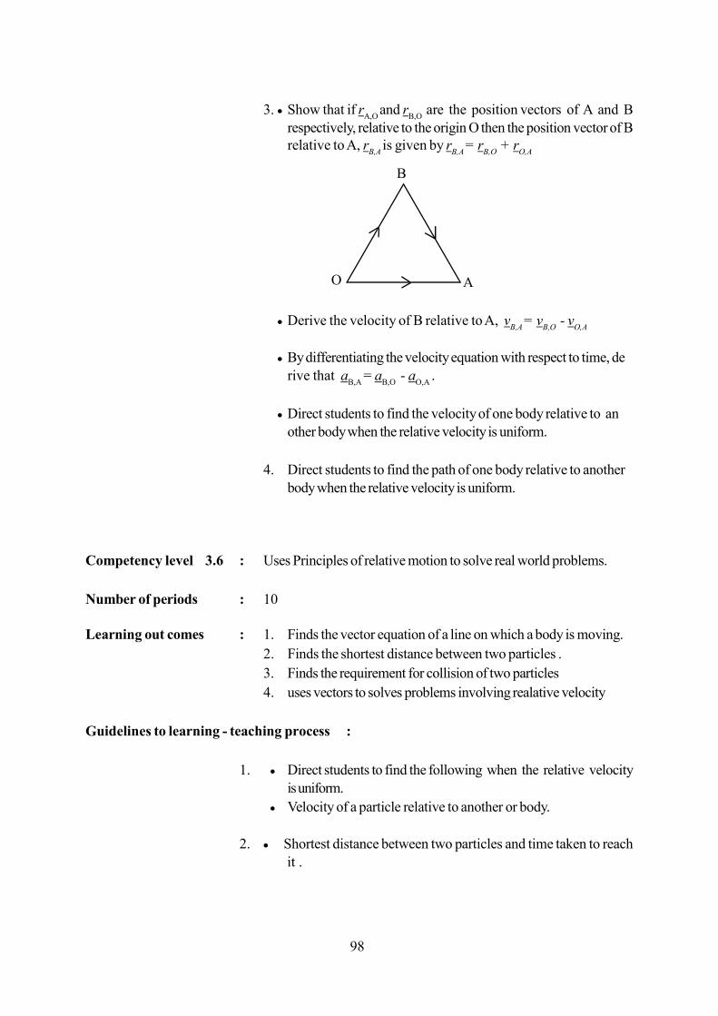
98

3. ² Show that if rA,O

and rB,O

are the position vectors of A and Brespectively, relative to the origin O then the position vector of Brelative to A, r

B,A is given by r

B,A = r

B,O + r

O,A

² Derive the velocity of B relative to A, vB,A

= vB,O

- vO,A

² By differentiating the velocity equation with respect to time, derive that a

B,A = a

B,O - a

O,A .

² Direct students to find the velocity of one body relative to another body when the relative velocity is uniform.

4. Direct students to find the path of one body relative to anotherbody when the relative velocity is uniform.

Competency level 3.6 : Uses Principles of relative motion to solve real world problems.


Learning out comes : 1. Finds the vector equation of a line on which a body is moving.

2. Finds the shortest distance between two particles .

3. Finds the requirement for collision of two particles

4. uses vectors to solves problems involving realative velocity


1. ² Direct students to find the following when the relative velocityis uniform.

² Velocity of a particle relative to another or body.

2. ² Shortest distance between two particles and time taken to reach it .

O A

B

99

3. ² The time taken to meat (If it so) and their position when they met.

² Time taken to conplete a given path.

4. ² Present solutions of problems involving motion relative to water or air.

² Guide students to solves problems using vectors.

Competency level 3.8 : Applies Newton’s laws to explain motion relative to an inertial frame


Learning outcomes : 1. States Newton’s first law of motion.

2. Defines “force”.

3. Defines “mass”.

4. Defines linear momentum of a particle.

5. States that linear momentum is a vector quantity.

6. States the dimensions and unit of linear momentum.

7. Describes an inertial frame of reference.

8. States Newton’s second law of motion.

9. Defines Newton as the absolute unit of force.

10. Derives the equation F ma from second law of motion.

11. Explains the vector nature of the equation F ma from second

law of motion.

12. States the gravitational units of force.

13. Explains the difference between mass and weight of a body.

14. Describes “action” and “reaction”.

15. States Newton’s third law of motion.

16. Solves problems using F ma

17. Bodies in contact and particles connected by light invetensible strings

18. Solves problems involving pullys

19. Solves problems involving wedges


1. A body continues to be in a state of rest, or of uniform motionalong a straight line, unless it is a acted upon by an external force.

2. Define ‘force’ as the external action that changes the state ofmotion of a body.

3. Define mass as the amount of response of the body to a forceacting on it.

100

4. Define linear momentum of a particle of mass m moving with avelocity u as mu.

5. Show that in the product mu, the velocity u is a vector and hencethe linear momentum is also a vector.

6. The dimensions of linear momentum are 1MLT .

Unit of linear momentum is 1kgms .

7. Describe an inertial frame of reference as a frame, which is atrest or moving with a uniform velocity relative to a frame of reference fixed on the earth.

[Earth is considered as an inertial frame of reference in studyingmotions taking place on Earth’s - surface.]

8. Tha rate of change of linear momentum of a body is directly

proportional to the external force. Derive F ma from

the second law.

9. The Newton is defined as the force required to produce an ac

celeration of 21 ms , on a mass of 1 kg . Introduce this as an

absolute unit of force.

10. From Newton’s second law of F k ma and according to the

definition of the Newton, show that 1k . Therefore F ma .

Hence m is measured in kilograms a in meters per second 2ms

then F is measured in Newtons.

11. According to F m a the acceleration takes place in the direc

tion of the force F. Show that the equation could be used by

resolving the force and the acceleration in any direction.

12. Introduce kg weight as the gravitational force with which a massof 1kg is pulled towards the earth, gravitational attraction.

13. Introduce that the mass of a body is the amount of mattercontained in it and that the weight of a body is the graviationalforce with which that body is attracted towards the earth. Statethat when the mass is measured in kg, and the acceleration due togravity is measured in ms-2 the units of weight is obtained in N.

14. Draw the attention of students to different types of forces - usingexamples show how forces always occur in pairs. For example,action and reaction between two bodies in contact.

101

15. “For every action between bodies, there is a reaction of equalmagnitude and opposite direction along the same line of action”

16. Solves problems using f = ma

17. Students are expected to solve problems related to followingcases.i. Find acceleration of a body under the action of given

external forces. Find external force when the accelerationis given . Find reaction between body and a lift, when thelift is moving with given acceleration. The acceleration produced by external forces acting on two bodies connectedby a string and the tension in the string.

ii. When forces act on a system of bodies, find the acceleration of each body of the system and reactions betweenbodies in the system.

iii. Calculate frictional forces acting, by considering themotion of a body on a rough plane.

iv. Problems relating to the motion of systems comprising ofconnected particles which have various accelerations orrigid bodies.

v. Motion of particle on a smooth wedge, which may (including smooth pulleys) moving on a smooth plane.

vi. External forces acting on two bodies which are connectedby a strings, obtain their acceleration and the tension.

18. Solves problems involving pullys

19. Solves problems involving wedges

Documents

Combined Mathematics - nie.lk Com Maths.pdf · reforms, Teachers' Guide for combine mathematics for grade 12 has been prepared. The grade 12 Teacher’s Guide has been organized under