Combined gravitational and electromagnetic self-force on charged particles in electrovac spacetimes part II Thomas Linz In collaboration with John Friedman

1

Combined gravitational and electromagnetic self-force on charged

particles in electrovac spacetimes part II

Thomas LinzIn collaboration with John Friedman and Alan Wiseman

http://arxiv.org/abs/1406.5112

2

Outline

• Electrovac• Angle-average renormalization• Solving for the singular field– “familiar” fields – “new” fields

• Mode-sum– Background– In electrovac

• Conclusions & Future Work

3

Outline




4

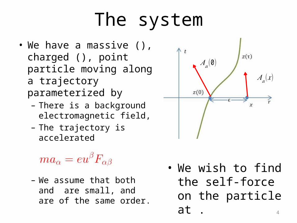
The system• We have a massive (),

charged (), point particle moving along a trajectory parameterized by – There is a background

electromagnetic field, – The trajectory is

accelerated

– We assume that both and are small, and are of the same order.

• We wish to find the self-force on the particle at .

𝐴𝛼(0)

𝐴𝛼(𝑥)

5

Field Equations• The background fields, satisfy the Einstein-Maxwell

Equations:

• We perturb these and solve for the perturbing fields ,

6

Perturbing The Field Equations

• Perturbing Einstein:

• Perturbing Maxwell:

7

Color-Coding

• JF used blue and red to distinguish terms that depended on the mass, m, and the charge, e.

• I use the colors differently:– RED = Equations or terms that are familiar.– BLUE = Equations or terms that are new

8

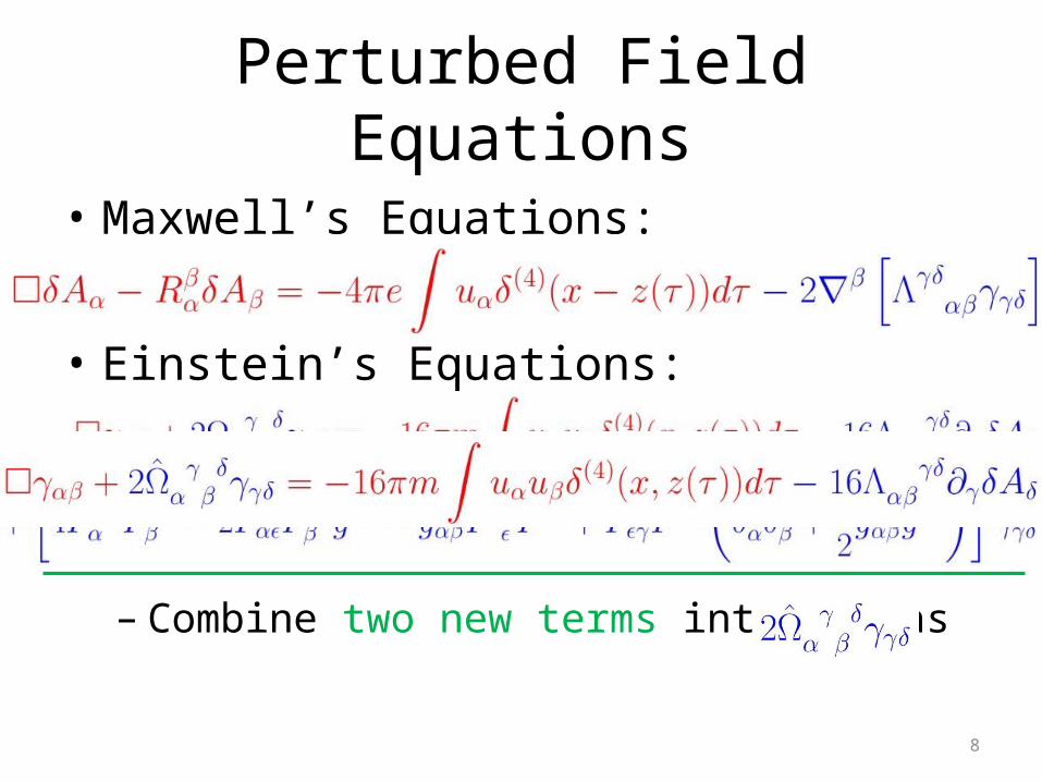
Perturbed Field Equations

• Maxwell’s Equations:

• Einstein’s Equations:

– Combine two new terms into one as

9

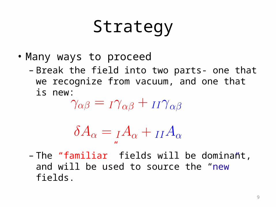
Strategy

• Many ways to proceed– Break the field into two parts- one that we

recognize from vacuum, and one that is new:

– The “familiar” fields will be dominant, and will be used to source the “new” fields.

10

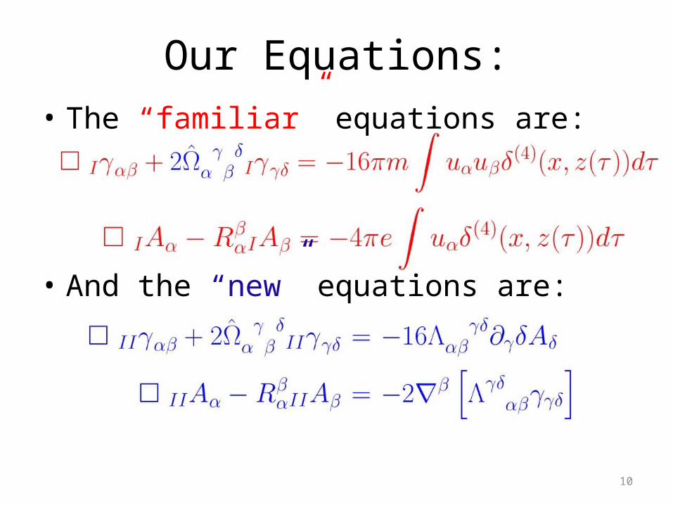
Our Equations:• The “familiar” equations are:

• And the “new” equations are:

11

Outline




12

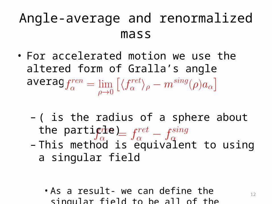
• For accelerated motion we use the altered form of Gralla’s angle average prescription:

– ( is the radius of a sphere about the particle)– This method is equivalent to using a singular field

• As a result- we can define the singular field to be all of the pieces of the retarded field that angle average away added to the mass renormalization term.

Angle-average and renormalized mass

13

Outline




14

Solving the “familiar” equations• These look (nearly) identical to the uncoupled

equations

– The electromagnetic four potential will look identical to the vacuum case.

– The only difference is the term instead of the Riemann Tensor

15

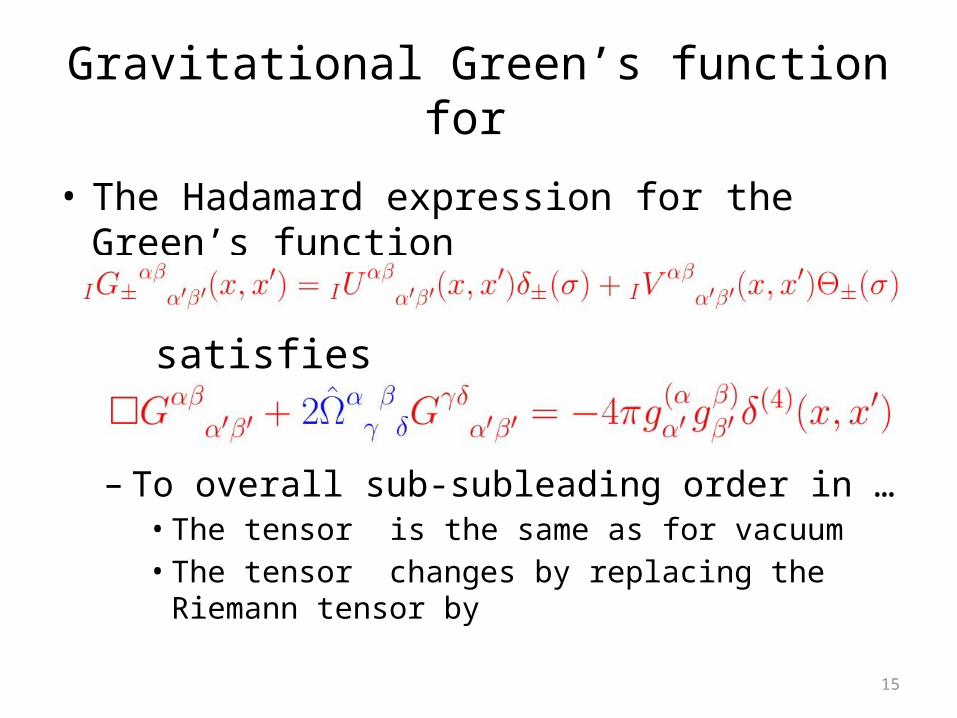
Gravitational Green’s function for

• The Hadamard expression for the Green’s function

satisfies

– To overall sub-subleading order in …• The tensor is the same as for vacuum• The tensor changes by replacing the Riemann tensor

by

16

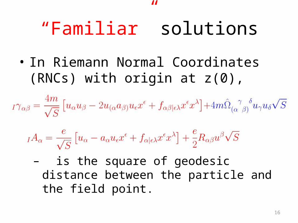
“Familiar” solutions

• In Riemann Normal Coordinates (RNCs) with origin at z(0),

– is the square of geodesic distance between the particle and the field point.

17

Outline




18

The “new” Equations

• The equations for the mixing terms are:

• We solve them iteratively, order by order in .– To first non-vanishing order, the fields are just

sourced by and .

19

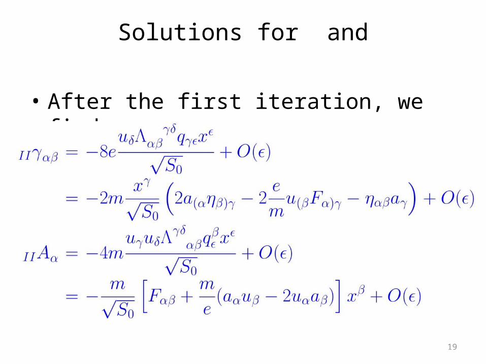
Solutions for and

• After the first iteration, we find:

20

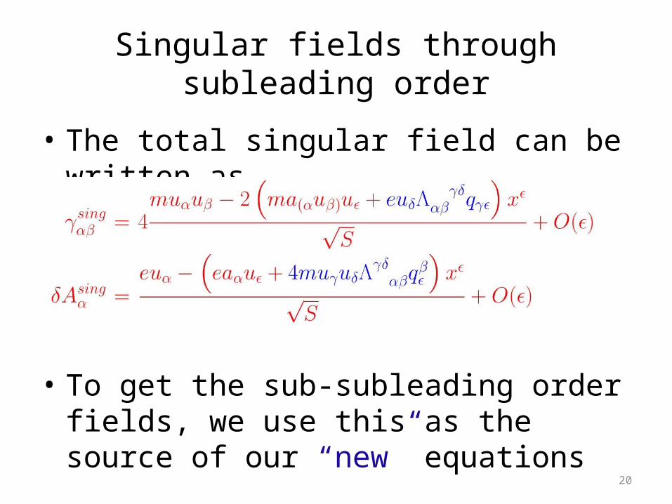
Singular fields through subleading order

• The total singular field can be written as

• To get the sub-subleading order fields, we use this as the source of our “new” equations

21

Uniqueness

• As discussed by JF, the fields are uniquely determined through subleading order.– Beyond that order, there is an ambiguity in the

fields.– There are homogeneous solutions which take on

the form of • Therefore any solutions we have could differ from the

singular field only by terms of this form.• We appear to be able to exclude these terms as well

22

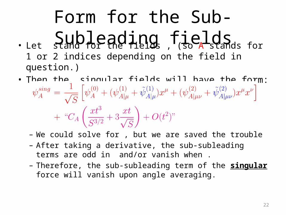
Form for the Sub-Subleading fields• Let stand for the fields , (so A stands for 1 or 2

indices depending on the field in question.)• Then the singular fields will have the form:

– We could solve for , but we are saved the trouble– After taking a derivative, the sub-subleading terms are odd

in and/or vanish when .– Therefore, the sub-subleading term of the singular force

will vanish upon angle averaging.

23

Outline




24

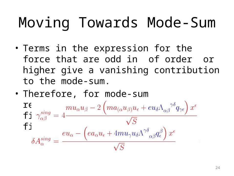
Moving Towards Mode-Sum

• Terms in the expression for the force that are odd in of order or higher give a vanishing contribution to the mode-sum.

• Therefore, for mode-sum regularization we keep only the first two terms in the singular field:

25

Mode-sum

• We decompose the retarded and singular fields into their harmonics:

• Then, after introducing a regulator, we perform the subtraction mode by mode.

26

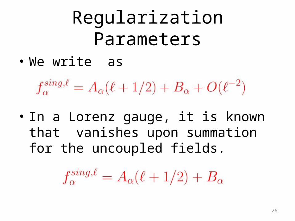
Regularization Parameters

• We write as

• In a Lorenz gauge, it is known that vanishes upon summation for the uncoupled fields.

27

Outline




28

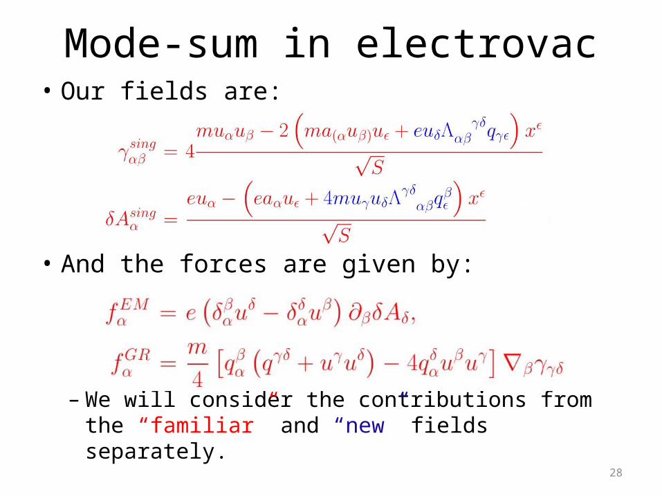
Mode-sum in electrovac• Our fields are:

• And the forces are given by:

– We will consider the contributions from the “familiar” and “new” fields separately.

29

RPs from the familiar Fields

• Recall that is identical to the singular field of an accelerated, massless charge.

• Also, is identical to the singular metric perturbation of an accelerated mass through subleading order. – Therefore, the contribution from the “familiar”

fields to the regularization parameters will simply be the regularization parameters we are familiar with from vacuum spacetimes.

30

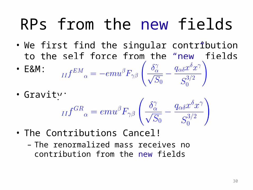
RPs from the new fields• We first find the singular contribution to the self

force from the “new” fields• E&M:

• Gravity:

• The Contributions Cancel!– The renormalized mass receives no contribution from the

new fields

31

Outline




32

Conclusions• We have provided a renormalization procedure for

electrovac– This can be extended for other types of non-vacuum

spacetimes.– It agrees with results of Zimmerman & Poisson

• They used two different methods, so that’s three different approaches that all agree.

• We have found the regularization parameters for mode-sum regularization– By a miraculous cancellation, they are merely the sum

of the separate electromagnetic and gravitational RPs.• (This will not be true of the higher order RPs, only the

“necessary ones.”)

33

Open Problems

• Justify by matched asymptotic expansions• Develop some type of generalization for non-

vacuum spacetimes• Explore the question of self-force acting as a

cosmic censor.• Find self-forces on uncharged point masses in

strong electromagnetic fields.– Comparison of self-force in Schwarzschild

spacetimes vs. Reissner-Nordström.

34

Thank you

Documents

Combined gravitational and electromagnetic self-force on charged particles in electrovac spacetimes part II Thomas Linz In collaboration with John Friedman