Combine Dimensional Analysis with Educated Guessing

Supplementary Material

Cedric J. Gommes∗

Dept. of Chemical Engineering, University of Liege, Belgium and

Funds for Scientific Research, F.R.S.-FNRS, Belgium

Tristan Gilet†

Dept. of Aerospace and Mechanical Engineering, University of Liege, Belgium

(Dated: January 24, 2018)

∗ cedric.gommes@uliege.be† tristan.gilet@uliege.be

1

CONTENTS

I. Pressure drop in a pipe (Hagen-Poiseuille law) 3

II. Pressure drop in a packing (Kozeny-Carman law) 6

III. Sedimentation of particles (Stokes’ law) 8

IV. Effusion of a gas (Graham’s law) 10

V. Binary diffusion in gases (Chapman-Enskog’s formula) 12

VI. Emulsification in a turbulent flow 15

VII. Effectiveness factor of a catalytic pellet (Thiele modulus) 19

2

I. PRESSURE DROP IN A PIPE (HAGEN-POISEUILLE LAW)

A fluid with density ρ [kg.m−3] and viscosity µ [kg.m−1.s−1] flows at a volume rate Q

[m3.s−1] through a pipe with length L [m] and radius R [m]. What is the pressure drop

∆P [kg.m−1.s−2] along the pipe? Perform first a dimensional analysis without any educated

guess, and then simplify it to the case of laminar flow.

Hint for guessing The pressure drop ∆P is expected to be proportional to the length L

of the pipe. Moreover, the density ρ should not play any role in the laminar regime.

FIG. I–1. The Hagen-Poiseuille problem. A viscous liquid flows in a cylindrical pipe of length L

and radius R: what is the relation between the pressure drop ∆P = P1 − P2 and the volume flow

rate Q?

Solution with no guessing. With dimensional variables the solution should take the

mathematical form

∆P = F (Q, ρ, µ, L,R) (I–1)

That is a total of 6 variables with 3 dimensions, i.e. 3 dimensionless groups of variables. We

already know at this stage that, whatever the solution is, it can can be put as

Π0 = F (Π1,Π2) (I–2)

where Π0, Π1 and Π2 are 3 dimensionless groups of variables, and F is an unknown function.

Equation (I–2) is already a great simplification compared to Eq. (I–1), because the number

of variables to be investigated in any experiment is reduced from 5 to 2.

There is no unique way to define the dimensionless groups Π, but it does not matter

because they are all equivalent in the end. A possibility consists in taking Q [m.s−3], ρ

3

[kg.m−3], and R [m] as core variables. They contain all the units (kg, m, and s) and they

can therefore be used to put the remaining variables (∆P , L, and µ) in dimensionless form.

At this step, some opportunistic reasoning is always useful. For example, one may recall

that ρ times velocity squared has the dimension of a pressure, which immediately suggests

the following dimensionless group

Π0 =∆P

ρ(Q/R2)2=R4∆P

ρQ2(I–3)

where Q/R2 has the dimensions of a velocity. Another dimensionless group is

Π1 =L

R(I–4)

The last group to be formed is based on the viscosity µ, which has the dimensions of pressure

times seconds. One can use again the group ρ(Q/R2)2 to create the pressure units, and R3/Q

to form the seconds. This yields

Π2 =µ

ρ(Q/R2)2R3/Q=Rµ

ρQ(I–5)

The law governing the flow of viscous liquid in a pipe has therefore to be

R4∆P

ρQ2= F

(L

R,Rµ

ρQ

)(I–6)

Solution with guessing. The two educated guesses here are (i) that the pressure drop

∆P should be proportional to the pipe length L and (ii) that density should not play a role

in the laminar regime. There are two ways to exploit these guesses. The first approach is

the one we followed in the main text, which consists in starting the analysis leading to Eq.

(I–6) all over again, only with variable ∆/L and without ρ. This leads to

∆P

L= F (Q, µ,R) (I–7)

There are 4 variables left and still 3 dimensions, so we are in the lucky situation where there

is a single dimensionless group of variables that cannot but be a constant.

Π0 = constant (I–8)

To find the expression of Π0 one can recall that the viscous stress, which is dimensionally

equivalent to µU/R where U is a velocity, has the dimension of a pressure. Using Q/R2 as

a group with the dimension of a velocity, this leads to

Π0 =∆P/L

µQ/R4(I–9)

4

Expressing that Π0 is a constant leads to

∆P

L= constant× µQ

R4(I–10)

which is the well-known form of the Hagen-Poiseuille law, with the distinctive R4 depen-

dence.

Another way to exploit the educated guessing is starting from Eq. (I–6). Because ∆P

has to be proportional to L, the unknown function F (Π1,Π2) has to be linear in Π1, which

leads toR4∆P

ρQ2=L

R× F1

(Rµ

ρQ

)(I–11)

where F1() is another unknown function. Moreover, because the density should not play

any role, the variable ρ has to disappear from Eq. (I–11). The only possibility is that

the function F1() be linear too, namely F1(Π2) = constant × Π2. This leads again to the

Hagen-Poiseuille law as in Eq.(I–10).

5

II. PRESSURE DROP IN A PACKING (KOZENY-CARMAN LAW)

Same question as in the Hagen-Poiseuille problem, only with the pipe filled with a pack-

ing of small grains with diameter d [m]. How does the pressure drop depend on the grain size?

Hint for guessing If the grains are much smaller than the pipe, the flow should be

homogeneous over the section. In other words, the relevant variable is not Q but Q/(πR2).

FIG. II–1. Permeability of a packed bed: the situation is identical to Fig. I–1 only with the pipe

filled with small grains, in the interstices of which the fluid can flow. How is the flow rate related

to the pressure drop?

Solution with no guessing With dimensional variables the solution should take the

mathematical form

∆P = F (Q, ρ, µ, L,R, d) (II–1)

That is a total of 7 variables with 3 dimensions, i.e. 4 dimensionless groups of variables.

Whatever the solution is, it can can be put as

Π0 = F (Π1,Π2,Π3) (II–2)

where Π0, Π1, Π2 and Π3 are 4 dimensionless groups of variables, and F is an unknown

function.

The first three dimensionless groups are identical to those identified in the Hagen-

Poiseuille problem, Eqs (I–3), (I–4) and (I–5), and the extra group is here

Π3 =d

R(II–3)

6

The general solution has to take the form

R4∆P

ρQ2= F

(L

R,Rµ

ρQ,d

R

)(II–4)

which is a generalisation of Eq. (I–6).

Solution with guessing For the same reasons as in the Hagen-Poiseuille case, the

unknown function F in Eq. (II–4) has to be linear in its first two arguments, namely

R4∆P

ρQ2=L

R× Rµ

ρQ× F1

(d

R

)(II–5)

where F1 is an unknown function of a single variable. Rewriting Eq. (II–5), it can be put

as∆P

L=µQ

R4× F1

(d

R

)(II–6)

If the grains are small enough, the flow of liquid should be homogeneous over the section of

the pipe. This means that if both the flow Q and the section R2 are doubled, the pressure

drop should remain the same. The relevant variable that should appear in Eq. (II–6) is

therefore Q/R2. This is only possible is F1 has the following dependence on its argument

F1 (Π3) = constant/Π23 (II–7)

The result is finally

∆P

L= constant× µQ/R2

d2(II–8)

which is nothing but Darcy’s law. One therefore recovers the result that the pressure drop

in a packing scales like the inverse square of the grain size.

Equation (II–6) can also be obtained by discarding/grouping dimensional variables from

the beginning. Discarding the density ρ from the very beginning, and introducing the

variables ∆P/L and Q/R2, the dimensional analysis would start from

∆P

L= F

(Q

R2, µ, d

)(II–9)

There are four dimensional variables and three dimensions, which leads to a single dimen-

sionless number

Π0 =(∆P/L)d2

µ(Q/R2)(II–10)

Expressing that Π0 is a constant leads to Eq. (II–8) again.

It is interesting to note that Eq. (II–6) contains both the Hagen-Poiseuille law (Eq. I–10)

and Darcy’s law (Eq. II–8) as particular cases. Whether one or the other law is obtained

depends on the particular form of the function F1(), which can be guessed.

7

III. SEDIMENTATION OF PARTICLES (STOKES’ LAW)

A small spherical object with radius R [m] and density ρ [kg.m−3] sinks slowly in a lighter

and viscous fluid with density ρ′ [kg.m−3] and viscosity µ[kg.m−1.s−1]. What is the settling

velocity U [m.s−1]?

Hint for guessing The variables ρ, ρ′ and g can only appear under the form (ρ− ρ′)× g.

Moreover, the settling speed should be proportional to gravity.

FIG. III–1. A spherical object with radius R sinks slowly in a viscous fluid. What is the sedimen-

tation velocity?

Solution with no guessing In a brutal approach (without any educated guess) one

would write the following dimensional relation

U = F (R, ρ, ρ′, g, µ) (III–1)

which contains 6 dimensional variables and 3 dimensions. It can therefore be expressed

in terms of 3 dimensionless groups. Using R, µ and g to put the remaining variables in

dimensionless form, one obtains the following dimensionless groups

Π0 =U√Rg

(III–2)

Π1 =ρR√Rg

µand Π2 =

ρ′R√Rg

µ(III–3)

The dimensionless relation is therefore

U√Rg

= F

(ρR√Rg

µ,ρ′R√Rg

µ

)(III–4)

8

where F () is as usual an unknown function.

Solution with guessing From our educated guesses, one has to assume that F (Π1,Π2) =

F1(Π1 − Π2) where F1() is an unknown function of a single argument. One is therefore left

withU√Rg

= F1

((ρ− ρ′)R

√Rg

µ

)(III–5)

The second guess is that the sedimentation velocity should be proportional to g, which

entails that F1() be a linear function. The final result is therefore

U = constant× (ρ− ρ′)R2g

µ(III–6)

which is exactly Stokes’ law. Solving the equations of fluid mechanics leads to the value 2/9

for the constant in Eq. (III–6). Although dimensional analysis in itself does not tell us any-

thing about the value of the constant, this is yet another illustration that the dimensionless

constants that naturally appear in this type of analysis are of order one.

Stokes’ law (Eq. III–6) can also be obtained by incorporating the educated guessing at

the very beginning of the dimensional analysis. In this case, instead of Eq. (III–1), one

could start withU

g= F (R, ρ− ρ′, µ) (III–7)

Choosing U/g as a dimensional variable is a way of enforcing the proportionality of U and g

in the final result. Equation (III–7) involves 4 variables and 3 dimensions. It can therefore

be expressed in terms of the single dimensionless group

Π0 =U/g

R2(ρ− ρ′)/µ(III–8)

which has to be constant. This leads again to Stokes’ law.

9

IV. EFFUSION OF A GAS (GRAHAM’S LAW)

There is a hole with diameter d [m2] in a reservoir containing gas at pressure P

[kg.m−1.s−2] temperature T [K], and molecular mass m [kg]. What is the so-called ef-

fusion rate, namely the rate N [s−1] at which molecules leave the reservoir?

Hint for guessing When the hole is so small that molecules leave the reservoir one at

a time, the effusion rate should be proportional to the area of the hole.

FIG. IV–1. A small hole with diameter d is made in a reservoir containing a gas at pressure P and

temperature T : what is the rate at which molecules leave the reservoir through the hole?

Solution with no guessing We shall start the analysis with

N = f(T, P,m, d, kB) (IV–1)

where we have added the Boltzmann constant kB [kg.m2.s−2.K−1] to the variables. Any

universal physical constants (Planck’s constant, the speed of light, etc.) can in principle

intervene in any dimensional relation. There is, however, no reason to include Planck’s

constant if quantum effects are not expected to play a role, or the speed of light in a non-

relativistic context, etc. Here Boltzmann’s constant should naturally be present because

effusion is a manifestation of molecular-scale thermal agitation. Moreover, in absence of kB

in the list variables it would be impossible to create a dimensionless group that would contain

the temperature. Had we not included kB, we would have reached the wrong conclusion that

effusion is independent of the temperature. In light of that, T and kB can only appear as the

thermal energy kBT [kg.m2.s−2], and we shall therefore start the analysis with the following

10

dimensional relation

N = f(kBT, P,m, d) (IV–2)

There are 5 variables and 3 dimensions, so 2 dimensionless numbers can be formed. There

is only one combination of kBT , m and d that has the same dimension as N , namely√(kBT/m)/d. The first dimensionless group is therefore

Π0 =Nd√kBT/m

(IV–3)

The second and last dimensionless group has to depend on pressure. Noting that P has the

dimension of an energy per unit volume, the second dimensionless group is found to be

Π1 =Pd3

kBT(IV–4)

The relation is thereforeNd√kBT/m

= F

(Pd3

kBT

)(IV–5)

As such, this result already contains Graham’s law, which states the rate of effusion is

inversely proportional to the square root of the molecular mass.

Solution with guessing The explicit dependence on the pressure and temperature can

be obtained by exploiting the educated guess that N should be proportional to the area of

the hole d2. As usual this can be done in two ways. The first way consist in starting from

Eq. (IV–5), and observing that the proportionality of N to d2 is possible only if the function

F () is linear. This immediately leads to

N = constant× Pd2√mkBT

(IV–6)

The other possibility consists in starting the analysis with N/d2 as a basic variable. In that

case, one has 4 variables and 3 dimensions, i.e. only one dimensionless number, namely

Π0 =N√mkBT

Pd2(IV–7)

Expressing that this number is equal to a constant, one finds Graham’s law (Eq. IV–6)

again. A detailed calculation based on kinetic theory of gases yields the value 1/√

2π ' 0.4

for the unspecified constant.

11

V. BINARY DIFFUSION IN GASES (CHAPMAN-ENSKOG’S FORMULA)

How does the binary diffusion coefficient DAB [m2.s−1] of two gases A and B depend on

the temperature T [K] and pressure P [kg.m−1.s−2], as well as on the diameters dA and dB

[m] and masses mA and mB [kg] of the molecules?

Hint for guessing The microscopic events responsible for the diffusion are two-body

collisions between molecules A and B. The relevant mass in this context is the reduced

mass 1/m = 1/mA +1/mB, and the molecular size plays a role via the collision cross-section

σ2 = (dA/2 + dB/2)2. One may also assume that the diffusion coefficient is inversely pro-

portional to the collision cross-section.

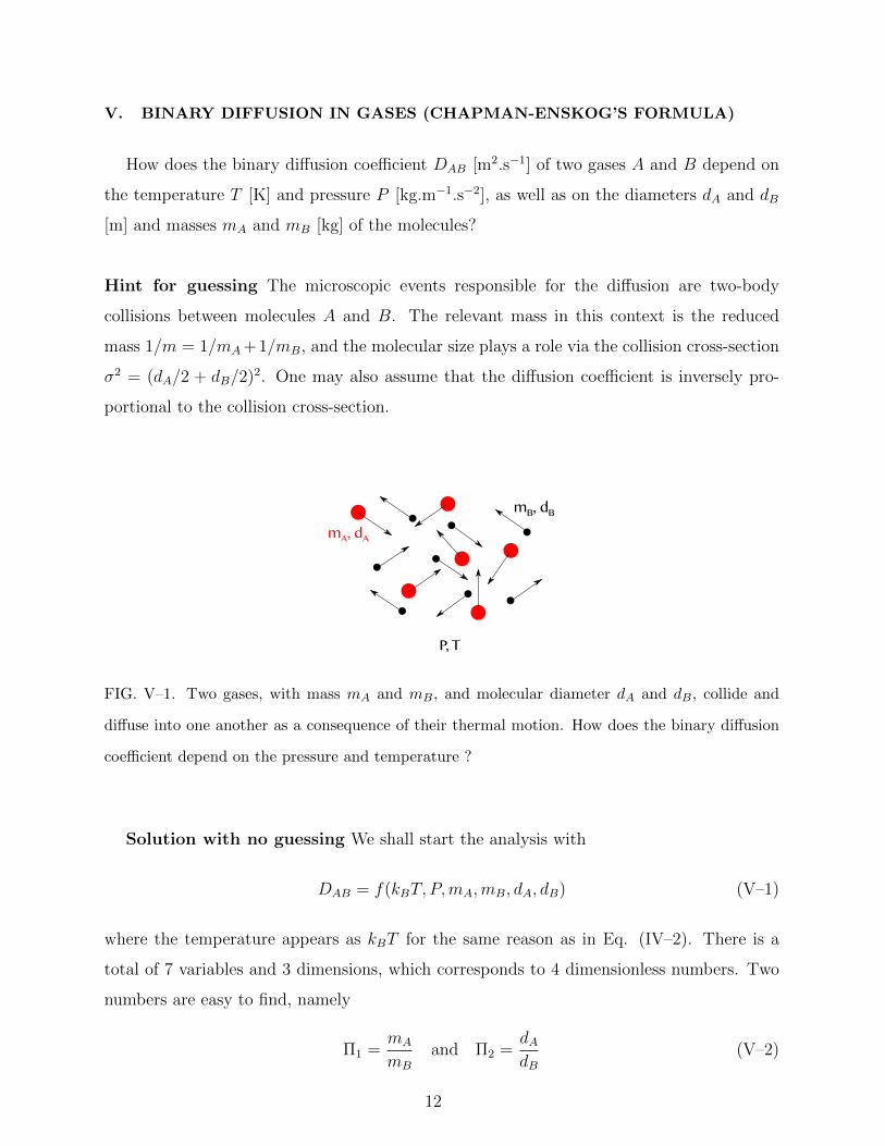
FIG. V–1. Two gases, with mass mA and mB, and molecular diameter dA and dB, collide and

diffuse into one another as a consequence of their thermal motion. How does the binary diffusion

coefficient depend on the pressure and temperature ?

Solution with no guessing We shall start the analysis with

DAB = f(kBT, P,mA,mB, dA, dB) (V–1)

where the temperature appears as kBT for the same reason as in Eq. (IV–2). There is a

total of 7 variables and 3 dimensions, which corresponds to 4 dimensionless numbers. Two

numbers are easy to find, namely

Π1 =mA

mB

and Π2 =dAdB

(V–2)

12

For the others, we first look for a combination of kBT , dA and mA that has the same

dimensions as DAB. The only solution is√kBTd2A/mA. This leads to the third number

Π0 =DAB√

kBTd2A/mA

(V–3)

One can create a last dimensionless number based on the pressure (which does not appear

in Π0, Π1 and Π2). That number is easily formed by noting that the pressure has the same

dimensions as an energy per unit volume, which lead to

Π3 =Pd3AkBT

(V–4)

The final result takes the form

DAB√kBTd2A/mA

= F

(mA

mB

,dAdB,Pd3AkBT

)(V–5)

This result is a bit obscure, but it already shows that diffusion scales as m−1/2, similarly to

effusion.

Solution with guessing In order to find the temperature and pressure dependence, it

is easier in this context to start the analysis over with the reduced mass

1

m=

1

mA

+1

mB

(V–6)

and with the collision cross-section σ2 [m2] as variables instead of mA, mB, dA and dB. The

relation is now

DAB = f(kBT, P,m, σ2) (V–7)

Because there are 5 variables and 3 dimensions, only two dimensionless numbers can be

formed. By analogy with Eqs. (V–3) and (V–4), a natural choice is

Π0 =DAB√kBTσ2/m

and Π1 =Pσ3

kBT(V–8)

yieldingDAB√kBTσ2/m

= F

(Pσ3

kBT

)(V–9)

If one assumes that the diffusion coefficient ought to be inversely proportional to the

collision cross-section σ2, the unknown function has to be of the type F (x) = constant/x,

which leads to

DAB = constant× (kBT )3/2

Pσ2√m

(V–10)

13

This is equivalent to the Chapman-Enskog expression of the binary diffusion coefficient.

The unknown dimensionless multiplicative constant is indeed of order one and it can be

calculated based on the so-called collision integral.

14

VI. EMULSIFICATION IN A TURBULENT FLOW

In an emulsification process two immiscible liquids, say water and oil (densities ρw and

ρo [kg.m−3], dynamic viscosities µw and µo [kg.m−1.s−1], and interfacial tension σ [kg.s−2]),

with total volumes Vw and Vo [m3] are mixed together in a container. The mixing is done

with a propeller of size D [m] that rotates at angular frequency Ω [s−1]. How does the

maximum size of the droplets d of the minority phase scale with Ω in the limit where the

mixing is so intense as to make the flow turbulent? (This example is inspired from Langmuir

28 (2012) pp 104-110.)

Hint for guessing Turbulence is reached for large values of the Reynolds number. The

relevant small-scale characteristic of a turbulent flow is the rate of energy dissipation per

unit mass of the fluid ε [m2s−3], quite independently of how that energy is provided to the

flow at large-scale.

FIG. VI–1. Water and oil are mixed together in a vessel with a propeller of size D rotating at

angular velocity Ω. How does the size d of the droplets that make up the emulsion depend on the

operating parameters?

Solution with no guessing Writing explicitly the dependence of d on all the variables

mentioned here above, one has

d = f (Vo, Vw, ρw, ρo, µw, µo, σ,D,Ω) (VI–1)

15

This sums up to 10 variables with 3 dimensions, yielding a total of 7 dimensionless numbers.

We define the first number as the dimensionless droplet size

Π0 =d

D(VI–2)

It is also natural to define the following two numbers as the ratio of the physical properties

of the two liquids

Π1 =µw

µo

and Π2 =ρwρo

(VI–3)

as well as the following number

Π3 =Vo

Vo + Vw(VI–4)

characterising the volume fraction of oil. We may define the fifth number as the dimensionless

size (or volume) of the propeller

Π4 =D3

Vo + Vw(VI–5)

As for the remaining two numbers, the Reynolds and Weber numbers are classical in this

context. The Reynolds number Re is the ratio of inertial forces to viscous forces. Using the

oil phase as a reference, the Reynolds could here be defined as

Π5 =ρoΩD

2

µo

(VI–6)

Similarly, the Weber number We is the ratio of the inertial forces to the capillary forces.

One may define it as

Π6 =ρoΩ

2D3

σ(VI–7)

With these dimensionless numbers, the relation becomes

d

D= F

(µw

µo

,ρwρo,

VoVo + Vw

,D3

Vo + Vw,ρoΩD

2

µo

,ρoΩ

2D3

σ

). (VI–8)

This equation is still uninformative, and the exact determination of F by experimental

means would be prohibitive. So once again, some guess is required to proceed further.

Solution with guessing In the limit of large values of the Reynolds number, typically

in turbulent conditions, the function F should no longer depend on Re. We can then write

d

D= F1

(µw

µo

,ρwρo,

VoVo + Vw

,D3

Vo + Vw,ρoΩ

2D3

σ

). (VI–9)

16

Moreover, the rate of energy dissipation per unit mass scales like ε = D2Ω3. Using that

expression, one can rewrite the Weber number in Eq. (VI–9) as

d

D= F1

(µw

µo

,ρwρo,

VoVo + Vw

,D3

Vo + Vw,ρoε

2/3D5/3

σ

). (VI–10)

For a given value of ε, the properties of the turbulent flow at the scale at which the droplets

form and coalesce are independent on the manner in which the energy is provided to the

flow. In particular, they are independent of the size of the propeller. This means that F1

cannot depend on D3/(Vo + Vw) and the dependence on the Weber number has to be of the

following type

d

D= F2

(µw

µo

,ρwρo,

VoVo + Vw

)×(ρoε

2/3D5/3

σ

)−3/5(VI–11)

where the exponent −3/5 is imposed by the fact that D has to cancel out in the left-hand and

right-hand sides. Note that the function F2 depends only on the quantities and properties of

the two immiscible liquids. As far as the propeller operation is concerned, F2 can therefore

be considered constant, yielding

d

D= constant×

(ρoΩ

2D3

σ

)−3/5. (VI–12)

A single experiment would be sufficient to determine the pre-factor of this scaling law.

We can then discuss the limit of validity of Eq. (VI–12), which depends on our assumption

of negligible viscous effects. As turbulence is multi-scale by nature, the relative importance

of inertial and viscous effects depends on the particular scale considered. At the scale of

the propeller, viscosity is negligible. However, this need not be the case at the scale of the

droplet. At the scale d of droplets, the relative importance of inertia and viscosity can be

quantified through an appropriate Reynolds number Rd. By construction, this number has

to be proportional to ρo/µo. It should also depend on the scale d. As the flow is turbulent,

its only relevant characteristic is the energy dissipation rate per unit mass ε. The only

dimensionless variable that can be formed according to these constraints is

Red =ρoε

1/3d4/3

µo

(VI–13)

Viscosity is then of negligible influence on the emulsification when Red > 1, which gives

when combined with Eq.(VI–12):

ε = D2Ω3 <ρoσ

4

µ5o

F20/32 (VI–14)

17

This yields a maximum operating rotation speed Ω, above which Eq.(VI–12) is no longer

valid.

18

VII. EFFECTIVENESS FACTOR OF A CATALYTIC PELLET (THIELE MODU-

LUS)

Many chemical reactions take place in porous solid catalysts into which the reactant

molecules have to diffuse before they can reach the active sites and react. Imagine a spheri-

cal catalyst pellet with radius R [m] and kinetic constant kV [s−1] per unit volume, in contact

with a reactant in concentration c [mol.m−3]. The diffusion coefficient of the reactant in the

pellet is D [m2.s−1]. What is the reaction rate N [mol.s−1] in the case where diffusion is

limiting the rate?

Hint for guessing When the reaction is diffusion-limited, it necessarily takes place close

to the surface of the pellet so that N is proportional to the area of the pellet.

Solution with no guessing The relation we look for is of the type

N = f (c, kV , R,D) (VII–1)

There are 5 variables based on 3 units ([mol], [m] and [s]), and the problem can therefore be

expressed in terms of only 2 dimensionless numbers. The first number can be obtained by

noting that the simplest combination of variables with the same dimension as N is R3kV c,

which leads to

Π0 =N

R3kV c(VII–2)

The second dimensionless number has to include the diffusion coefficient D [m2.s−1] in its

definition. It can be put in dimensionless form in the following way

Π1 =D

R2kV(VII–3)

The solution of the reaction-diffusion problem can therefore be put as

N

R3kV c= F

(D

R2kV

)(VII–4)

Solution with guessing In the diffusion-limited regime, the reactant molecules do not

have enough time to diffuse to the center of the pellet before they react. Because the reaction

only occurs close to the surface, N has to be proportional to the outer area of the pellet,

19

FIG. VII–1. Qualitative concentration distribution in a catalytic pellet of arbitrary shape (left) for

large reaction rates: the concentration decreases in a thin region close to the surface. The thickness

δ of that region can be defined precisely by extrapolating the profile as shown on the right.

i.e. to R2. This means that the analytical form of the function F () in Eq. (VII–4) has to

be F (Π1) = constant×√

Π1. The final result is therefore

N

R3kV c= constant×

√D

R2kV(VII–5)

This result is usually expressed slightly differently, in terms of the effectiveness factor

η =N

4/3πR3kV c=

3

4πΠ0 (VII–6)

which is the ratio of N and the reaction rate that would be obtained in the case where

diffusion would be much faster than reaction. In that case the concentration would be

homogeneous over entire catalyst pellet and equal to the external value c, so that N =

4/3πR3kV c. Moreover, one also defines the Thiele modulus φ as

φ =

√kVR2

D= 1/

√Π1 (VII–7)

In terms of these new dimensionless numbers, Eq. (VII–5) can be written as

η =constant

φ(VII–8)

which is a classical result of chemical engineering. The full solution of the problem, obtained

by solving the reaction/diffusion equation is spherical coordinates yields the exact value

constant = 3, which is of order of unity as expected.

The analysis here above concerned a spherical pellet, but it can be generalised to pellets

of any shape as sketched in Fig. VII–1. In the case where the reaction is faster than the

20

time needed for a molecule to diffuse over a distance comparable to the size of the pellet, the

concentration profile is expected to be as in Fig. VII–1. There is a thin layer of thickness

δ where the concentration is finite and further away from the surface the concentration is

practically zero. If necessary, δ can be defined rigorously as the intercept of the concentration

profile as shown in Fig. VII–1.The general dependence of δ is the following

δ = f(D, c, kV , L) (VII–9)

where L is a characteristic size of the pellet. In the case of a pellet with arbitrary shape, L

can be estimated as V/A where V and A are the pellet volume and outer area, respectively.

In the limit of fast reaction, however, the layer is so thin that we do not expect the shape

or size of the pellet to matter at all. In this limit the dependence becomes much simpler

δ = f(D, c, kV ) (VII–10)

Because L is no longer among the variables, there are only 4 variables and 3 dimensions

left. There is therefore a single dimensionless number, which is conveniently written as

Π0 = δ/√D/kV . Buckingham’s theorem therefore leads to

δ = constant×√D

kV(VII–11)

where the unknown constant is, as usual, expected to be of the order of unity.

Because we have defined δ in terms of the concentration gradient, the total number of

molecules that diffuse into the catalyst pellet can be written as

N = ADc

δ(VII–12)

were A is the outer area of the pellet, without any unknown dimensionless constant. Be-

cause we have assumed that the catalyst is working in stationary conditions, the number of

molecules that diffuse into the pellet is equal to the number of molecules that react inside

the pellet. So N has the same meaning as before. On the other hand, the effectiveness

factor for a pellet of arbitrary shape is defined as a function of the volume as follows

η =N

V kV c(VII–13)

Putting Eqs. (VII–11) and (VII–13) together yields the result

η =1

constant

1

φ′(VII–14)

21

10−1

100

101

10−1

100

φ’ η

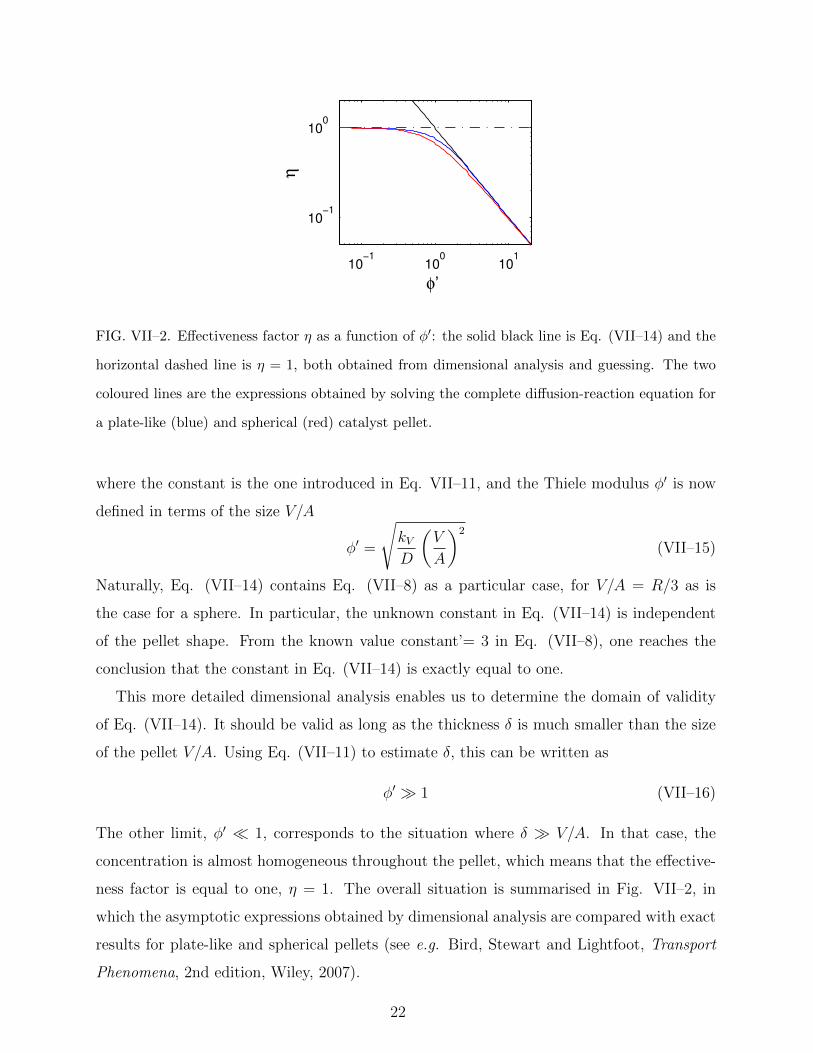
FIG. VII–2. Effectiveness factor η as a function of φ′: the solid black line is Eq. (VII–14) and the

horizontal dashed line is η = 1, both obtained from dimensional analysis and guessing. The two

coloured lines are the expressions obtained by solving the complete diffusion-reaction equation for

a plate-like (blue) and spherical (red) catalyst pellet.

where the constant is the one introduced in Eq. VII–11, and the Thiele modulus φ′ is now

defined in terms of the size V/A

φ′ =

√kVD

(V

A

)2

(VII–15)

Naturally, Eq. (VII–14) contains Eq. (VII–8) as a particular case, for V/A = R/3 as is

the case for a sphere. In particular, the unknown constant in Eq. (VII–14) is independent

of the pellet shape. From the known value constant’= 3 in Eq. (VII–8), one reaches the

conclusion that the constant in Eq. (VII–14) is exactly equal to one.

This more detailed dimensional analysis enables us to determine the domain of validity

of Eq. (VII–14). It should be valid as long as the thickness δ is much smaller than the size

of the pellet V/A. Using Eq. (VII–11) to estimate δ, this can be written as

φ′ 1 (VII–16)

The other limit, φ′ 1, corresponds to the situation where δ V/A. In that case, the

concentration is almost homogeneous throughout the pellet, which means that the effective-

ness factor is equal to one, η = 1. The overall situation is summarised in Fig. VII–2, in

which the asymptotic expressions obtained by dimensional analysis are compared with exact

results for plate-like and spherical pellets (see e.g. Bird, Stewart and Lightfoot, Transport

Phenomena, 2nd edition, Wiley, 2007).

22

The asymptotic behaviours of the curve are universal; they do not depend on the shape

of the pellet, however complicated it may be. The shape of the pellet only influences the

curve η(φ′) in the region φ′ ∼ 1 where both large-φ′ and small-φ′ asymptotes cross each

other.

23