Combination of ﬁnite element and reliability methods in

Combination of finite element and reliability methods in nonlinearfracture mechanics

M. Pendolaa,* , A. Mohamedb, M. Lemaireb, P. Horneta

aEDF-DRD, Mechanics and Technology Department, 77818 Moret-sur-Loing Cedex, FrancebLaRAMA-IFMA/UBP, BP 265, 63175 Aubiere Cedex, France

Received 27 July 1998; accepted 15 March 2000

Abstract

This paper presents a probabilistic methodology for nonlinear fracture analysis in order to get decisive help for the reparation andfunctioning optimization of general cracked structures. It involves nonlinear finite element analysis. Two methods are studied for thecoupling of finite element with reliability software: the direct method and the quadratic response surface method. To ensure the responsesurface efficiency, we introduce new quality measures in the convergence scheme. An example of a cracked pipe is presented to illustrate theproposed methodology. The results show that the methodology is able to give accurate probabilistic characterization of theJ-integral inelastic–plastic fracture mechanics without obvious time consumption. By introducing an “analysis re-using” technique, we show how theresponse surface method becomes cost attractive in case of incremental finite element analysis.q 2000 Elsevier Science Ltd. All rightsreserved.

Keywords: Structural reliability; Direct coupling method; Quadratic response surface method; Pipe; Finite element analysis; Nonlinear fracture mechanics

1. Introduction

The finite element method represents the most importanttool for structural analysis and design. Its applications areincreasing and its progress offers solutions to a wide varietyof problems such as three-dimensional (3D) structuralanalysis and nonlinear behavior. In the meantime, methodsbased on the probability theory have also been put forwardto try to quantify the influence of data uncertainties. Theynow offer some techniques of practical application by intro-ducing some approximations in the mechanical systemswhere the validity domain can be well defined.

In case of cracked components, the Linear Elastic Frac-ture Mechanics theory (LEFM) and the Elastic–PlasticFracture Mechanics (EPFM) provide accurate deterministicrelationship between the maximum allowable external load-ing and the component parameters: dimensions, materialproperties, crack size and location. However, due to uncer-tainties in some of these parameters (for instance, crack sizeand material properties), a purely deterministic approachprovides an incomplete picture of the reality. Therefore, aprobabilistic approach seems to be very helpful for practicalengineering and especially for the nuclear field: with the

goal to decide when a repair is necessary, it is interesting toknow the probability of failure of a damaged structuresubjected to a possible accidental load effect. Suchapproaches, namedprobabilistic fracture mechanicsarethen particularly interesting for taking into account the uncer-tainties related to the structure during the stage of design or inoperation to optimize the functioning conditions.

In many cases, the structural load effect cannot beexpressed explicitly and some finite element calculationsare necessary. Coupling of finite element analyses (FEA)with reliability methods is therefore necessary but impliesdifficulties such as prohibitive computation effort.

This paper deals with the case of coupling nonlinear frac-ture models with reliability methods, that is to say showingthe interest of performing a complex mechanical study in areliability context. From a mechanical point of view, onlystatic behavior is considered and the reliability modelconcerns random variables but not random fields and timeindexed stochastic processes.

The nonlinear fracture model is presented in the scope ofthe analysis of an axisymmetrically cracked pipe under pres-sure and tension with confined plastic behavior (i.e. theligament is not fully plastified). Two reliability methodsare used in the evaluation of the pipe safety: direct couplingand Quadratic Response Surface (QRS) method. Thisproblem has been analyzed by other authors (see for

Reliability Engineering and System Safety 70 (2000) 15–27

0951-8320/00/$ - see front matterq 2000 Elsevier Science Ltd. All rights reserved.PII: S0951-8320(00)00043-0

www.elsevier.com/locate/ress

* Corresponding author. Tel.:133-1-6073-7748; fax:133-1-6073-6559.E-mail address:[email protected] (M. Pendola).

example Ref. [6]), but here emphasis is laid on the compu-tation costs that can be largely decreased by optimal re-usingof all the incremental analysis performed in the finite elementcode due to the nonlinear behavior. We also propose somemeasures for the precision of the approximated response. Theresults from this example show that the methodology is ableto give accurate probabilistic characterization of the structureintegrity in the field of elastic–plastic fracture mechanics.Contrary to single reliability analysis, the efficiency of theQRS method is proven in parametric analysis which is veryinteresting in real industrial projects.

2. Mechanical model

2.1. General assumptions

Many existing structures or mechanical components have

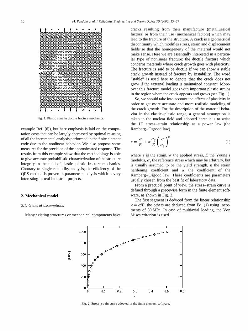
cracks resulting from their manufacture (metallurgicalfactors) or from their use (mechanical factors) which maylead to the fracture of the structure. A crack is a geometricaldiscontinuity which modifies stress, strain and displacementfields so that the homogeneity of the material would notmake sense. Here we are essentially interested in a particu-lar type of nonlinear fracture: the ductile fracture whichconcerns materials where crack growth goes with plasticity.The fracture is said to be ductile if we can show a stablecrack growth instead of fracture by instability. The word“stable” is used here to denote that the crack does notgrow if the external loading is maintained constant. More-over this fracture model goes with important plastic strainsin the region where the crack appears and grows (see Fig. 1).

So, we should take into account the effects of plasticity inorder to get more accurate and more realistic modeling ofthe crack growth. For the description of the material beha-vior in the elastic–plastic range, a general assumption istaken in the nuclear field and adopted here: it is to writethe 1D stress–strain relationship as a power law (theRamberg–Osgood law)

e � s

E1 a

sy

Es

sy

!n

�1�

wheree is the strain,s the applied stress,E the Young’smodulus,s y the reference stress which may be arbitrary, butis usually assumed to be the yield strength,n the strainhardening coefficient anda the coefficient of theRamberg–Osgood law. These coefficients are parametersusually chosen from the best fit of laboratory data.

From a practical point of view, the stress–strain curve isdefined through a piecewise form in the finite element soft-ware, as shown in Fig. 2.

The first segment is deduced from the linear relationshipe � s=E; the others are deduced from Eq. (1) using incre-ments of 50 MPa. In case of multiaxial loading, the VonMises criterion is used.

M. Pendola et al. / Reliability Engineering and System Safety 70 (2000) 15–2716

Fig. 1. Plastic zone in ductile fracture mechanics.

Fig. 2. Stress–strain curve adopted in the finite element software.

2.2. Loading effect characterization

There are several ways to characterize the stress fieldsingularity in the vicinity of the crack tip [27]: exact solu-tions are only known for special cases but the developmentsbased on the energy conservation laws are particularly inter-esting for nonlinear fracture mechanics. The crack growth isgoverned by the strain energy release rate indicating theenergy dissipation during the material separation (i.e. break-ing of cohesive forces between particles). In the generalcase, theJ-integral, whose formulation is based on energyconsiderations, is a very good measure of the crack drivingforces [12,25]. In nonlinear behavior, theJ-integral isknown to be path independent as long as the path remainsfar enough from the plastic region and loading is monotonicincreasing (local unloading is not taken into account). Eq.(2) gives the expression of theJ-integral in 2D form [25]. Itassumes that the crack lies in the global Cartesianx–y plane,with the x-axis parallel to the crack (see Fig. 3)

J �ZG

W dy 2ZG

tx2ux

2x1 ty

2uy

2y

� �ds �2�

whereG is any path surrounding the crack tip,W is the strainenergy density (i.e. strain energy per unit volume),tx thetension vector alongx-axis �� sxnx 1 sxyny�; ty the tensionvector alongy-axis �� syny 1 sxynx�; s the stress compo-

nents,n the unit outer normal vector to the pathG , u thedisplacement vector, ands the distance along the pathG .

2.2.1. Finite element implementation

2.2.1.1. Meshes associated with fracture modeling.One ofthe greatest difficulties in fracture mechanics is the meshrefinement which has to account for the singular stressand displacement fields at the crack tip. The evaluation oftheJ-integral needs a high precision which implies adaptedmeshing:

• either a refined mesh which converges at the crack tip.We can use quadratic elements at the crack tip withlength between 1/500 and 1/50 of the crack length;

• or the use of Barsoum’s elements where the midsidenodes are placed at the quarter points. Such elementsinduce the same singularity as the searched fields.

2.2.1.2. Numerical evaluation of the J-integral.The J-integral computation is carried out by the softwareANSYS [2] and Code_Aster [7] in order to have avalidation of the mechanical results by comparison.

With ANSYS, the J-integral is directly evaluated byconsidering Eq. (2):

• The path is chosen far enough from the crack tip to avoiderrors due to the singularity.

• The derivatives of the displacement vector are calculatedby shifting the path a small distance in the positive andnegativeX directions.

• The stresses and the strains are evaluated along the pathG defined by nodes, that is to say we use an interpolationprocess from the known values at the Gauss points.

With the softwareCode_Aster[7], the crack driving forceevaluation is implemented through the use of theu -methoddeveloped by the French company Electricite de France(EDF). This method considers the exact derivatives of thedisplacement field by rewriting the variational formulations.

2.3. Characterization of the structural strength

In order to evaluate the structural integrity, relevant fail-ure criteria must be defined. Two definitions are commonlyused in the EPFM [14]: (i) initiation of crack growth; and(ii) unstable crack growth. The initiation of crack growth ina structure containing flaws is observed when the crackdriving forceJ exceeds the material toughness (JIc) depend-ing only on the material. This criterion is commonly used inpiping and pressure vessel analyses [23]. Otherwise thiscriterion provides a conservative estimate of the structuralintegrity because after crack growth initiation there isunstable crack growth. This criterion is used in the currentfracture analysis.

The crack initiation in ductile elastic-plastic environments

M. Pendola et al. / Reliability Engineering and System Safety 70 (2000) 15–27 17

Fig. 3. Integration path surrounding the crack tip.

Fig. 4. Definition ofJ0.2 according to ASTM E 813 [3].

is thus obtained when Rice’s integral reaches the materialtoughnessJ0.2. This value results from experimentation. Theindex 0.2 means 0.2 mm, i.e. the toughness is defined for a0.2 mm crack propagation.J0.2 is then the value defined bythe intersection between the regression curve due to theexperimental points and the parallel to the blunting linedefined by the equationJ � 2sfDa (Fig. 4) wheres f isthe flow stress defined by the mean of the yield stress andthe maximal stress.

2.4. Remarks on mechanical modeling

Fracture mechanics is based on assumptions and formu-lations which may lead to accurate and realistic modeling ofthe cracking phenomena but which still requires heavycomputation efforts. The main problem is therefore topilot the finite element calculations in a nonlinear contextwhen a parametric reliability analysis has to be performed(multiplication of the FEA computations is required). Assingle FEA requires several minutes and as the expectedprobability of failure is generally very small, the classicalMonte Carlo simulations cannot be reasonably used. Specialcoupling approaches for reliability methods and finiteelement analyses have to be considered.

3. Coupling finite element with reliability methods

The main reliability methods used in our study are basedon FORM/SORM (First/Second Order Reliability Meth-ods). Different approaches have been proposed and two ofthem are used here. The first one is based on the computa-tion of the Hasofer and Lindb index [17] for an approx-imate form of the loading effect given by a response surface.The second approach is based on a direct computation of thereliability index using FEA by optimization procedures.This second method which requires a link between the finiteelement and reliability software has been essentially used tovalidate the first one which does not need significantprogramming cost.

3.1. Reliability problem—notations

Let xi be a realization of the random variableXi (i varyingfrom 1 to the number of basic variablesN) and G�xi� theperformance function

G�xi� . 0 is a success realization,xi [ Ds; safetydomain;G�xi� # 0 is a failure realization,xi [ Df ; failure domain;G�xi� � 0 is the limit state.

The probabilistic transformationT gives for any physicalvectorXi, the standardized vectorUj of Gaussian variablesN(0,1). The Nataf transformation [8], that requires onlylimited information (generally available) on variablesXi

(marginal densities and correlation), constitutes an efficient

solution. It is thus

ui � Ti�xj� G�xi� � G�T21i �uj�� ; H�uj� �3�

The Hasofer–Lind reliability indexb is then calculated bysolving the optimization problem

b � min

��XNi�1

u2i

vuut0@ 1A under the constraintH�ui� # 0 �4�

The solution gives the value ofb and the coordinatesuip of

the design pointPp as well as the direction cosinesa i (sensi-tivity factors in the standardized space).

3.2. Direct coupling method

By the direct coupling method, we mean any reliabilityprocedure based on ab -point search algorithm usingdirectly the FEA each time the limit state function has tobe evaluated. Theb -point search can be carried out by anyoptimization method allowing to solve Eq. (4).

By using the gradient based algorithms, there is no needto know the closed-form of the limit state function to deter-mine the failure probability. All that we need are the valuesof the limit state and its gradient (and may be the Hessian) atthe computation points. Historically, the Rackwitz andFiessler algorithm [22] has been frequently used in reliabil-ity analysis but some instability problems were observed.The convergence rate has been well improved by the Abdoand Rackwitz algorithm which is a simplified form of thesequential quadratic programming algorithm [1]. As forthe most of optimization methods, there is no guaranteethat the calculated minimum is really the global minimumof the problem; only good engineering sense allows us to geta logical interpretation of the coherence of the failureconfiguration.

3.3. Quadratic response surface method

In many industrial cases, the structural failure cannot bedefined by an explicit function of the random variables; onlyan implicit definition of the limit stateG is available. Thesolution can be obtained by the construction of the responsesurface (RS) based on a limited number of realizations inorder to obtain the approximation of the limit state function.The use of response surfaces in reliability problems is notrecent, but has not been achieved and new contributions arealways proposed. Works have defined concepts[5,11,19,24], built solutions in the physical space [4],proposed methods of evolution [10,13] and showed applica-tions with finite element coupling [6,26]. It is emphasizedhere on a method proposed by [9] and based on an approx-imation of the limit state in the vicinity of the design pointdetermined after successive iterations.

3.3.1. Quadratic response surface evaluationThe main idea of the response surface method is to build a


polynomial expansion of the limit state functionG�xi� orH�ui�: The degree 2 (Quadratic Response Surface, QRS) isthe best solution since it includes a possible calculation ofcurvatures and it avoids possible oscillations of higher orderpolynomials. We choose to built the approximation in thestandardized space. If there areN random variables in thestandardized space, the approximation~H�ui� of H�ui� can bewritten as

~H�ui� � c 1XNi�1

biui 1XNi�1

XNj�i

aij uiuj �5�

wherec, bi andaij are constants to be determined. The func-tion ~H�ui� is defined by at leastrmin � �N 1 1��N 1 2�=2points but in practice a larger numberr of points is takenand the approximation is obtained by minimizing the leastsquaresXr

l�1

u ~H�u�l�i �2 H�u�l�i �u2 �6�

At the iteration “h”, the construction of the polynomialapproximation is done by choosing carefully the set (k) ofrealizations of the implicit functionH�ui�: The equation~H�ui� � 0 enables us to calculate an estimation ofb�k�

and the most probable failure pointuip. A new polyno-

mial approximation (k 1 1) is obtained from the evalua-tion of the implicit function located in the vicinity ofup�k�

i and eventually some of the previous realizations ofthe implicit function stored in the database. Severaliterations allow us to approach the limit state functionand to calculate the indexb . The convergence isachieved, with the same conditions as in the directcoupling method, when

ub�k11� 2 b�k�u # eb �7�

H�{ u} �k11��H�{0} �

�� # eH �8�

where eb and eH are, respectively, the convergencetolerance forb and H. To avoid error redistributionbetween the design point components, an additionalcondition should be applied on the normalized variablecomponents

uu�k11�i 2 u�k�i u # eu �9�

wheree u is the convergence tolerance forui. The re-useof the nearest points obtained in the previous iterationdecreases the number of finite element computations andthereby the global computation cost [21].

3.3.2. Quality of the RSThe main problem in the response surface analysis is the

validation of the obtained results and approximations. Thereare tests giving measures on the quality of the approxima-

tions. They can be classified according to the necessaryinformation for their evaluation [15]

• Physically admissible realizations.We build theresponse surface in the standard space. The choice of arealization u�l�j implies a physical realizationx�l�i �T21

i �u�l�j � that must be physically feasible and corre-sponds to a compatible situation with the mechanicalmodel hypotheses. If not, the aberrant realization isexcluded from the set of experiments. When the coeffi-cients of variation are relatively small there is always aphysical realization in the considered probability domain.This verification has to be performed only when the scat-ter of the variable is great in order to avoid aberrantcomputations.

• Quality of the regression.It is measured after the calcu-lation of the realizations~H�u�l�i �: The measure is thecorrelationR2 between real limit state and the polynomialapproximation calculated at the pointsu�l�i

R2 � 1 2

Xr

l�1

�H�u�l�i �2 ~H�u�l�i ��2Xr

l�1

�E�H�u�l�i ��2 H�u�l�i ��2! 1

in which E[·] is the average. This measure is equal to 1for an interpolation and must be used only to control theregression where a value superior to 0.95 is expected. Ifthe statisticR2 is less than 0.95, it means that the regres-sion does not consider all the available informationcontained in the numerical experiments. In such cases,experience shows that taking into account more numer-ical experiments leads to better approximations.

• Value of the limit state function.At the end of the relia-bility calculation, the design pointPp is obtained. Wepropose two supplementary measures [21]◦ the first measure checks the belonging ofPp to the

design of experiments

Iapp� 1 21r

Xj

t�1

Nt

t!

!21

! 1

wherej is the chosen limit for the development andNt

is the number of the set of experiments points to beless thant standard deviations ofPp according to agiven norm

Nt � card�P�l�u maxi�1;N

�u�l�i 2 ~upi � , t�

or

Nt � card P�l��

��XNi�1

�u�l�i 2 ~upi �2

vuut , t�

◦ the second measure verifies that the design point


belongs to the real limit state function (see Eq. (8))

Ia � H�{ ~up} �H�{0} � ! 0

It requires a supplementary mechanical calculationand if it tests the belonging to the limit state, it doesnot prove that it is a minimum on the limit state func-tion. However experience [21] shows that good relia-bility results are strongly correlated with a goodmeasure ofIa, and reciprocally.

4. Application to a cracked pipe

4.1. Description of the pipe

The pipes of nuclear plants undergo great thermal andmechanical cycles which can lead to initiation and propaga-tion of cracks. When a crack is observed, the problem is toknow whether it is suitable to repair the structure as a prior-ity or if it can be justified that an accident will not occur.Therefore, the reliability analysis can provide the failureprobability knowing that there is a crack and that the loadcan reach accidental values defined in a particular range.

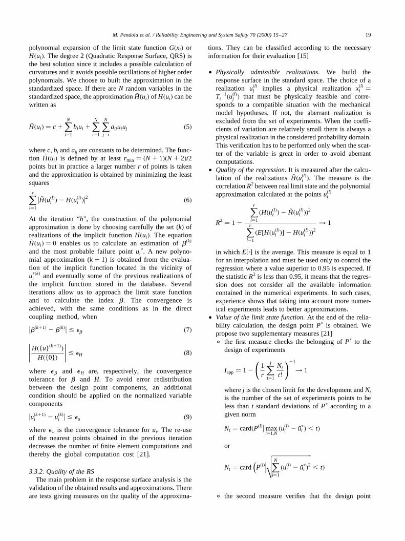
Fig. 5 shows an axisymmetrically cracked pipe underinternal pressure and axial tension. Due to the boundaryconditions at the pipe ends, the applied hydraulic pressureinduces, beside the radial pressure, longitudinal tensionforces.

The system variables are described as follows:

• a, the crack length (15 mm)• L, the pipe length (1000 mm)

• P, the internal pressure (15.5 MPa)• Ri, the inner radius (393.5 mm)• t, the thickness (62.5 mm)• s t, the applied tensile stress (varying from 100 up to

200 MPa). It represents the load effect which could acci-dentally increase, knowing that the nominal value isaround 100 MPa. This load is taken as a deterministicparameter in the reliability analysis, that is to say weare interested in obtaining the failure probability as afunction of the tensile stress in order to be able to decideif pipe repairing has to be done with acceptable failureprobability for a given crack length and loading effect.

• s0, the stress due to the end effects, given by

s0 � PR2

i

�Ri 1 t�2 2 R2i

4.2. Finite element model

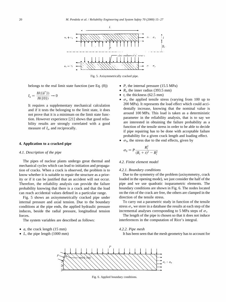
4.2.1. Boundary conditionsDue to the symmetry of the problem (axisymmetry, crack

loaded in the opening mode), we just consider the half of thepipe and we use quadratic isoparametric elements. Theboundary conditions are shown in Fig. 6. The nodes locatedon the rim of the crack are free, the others are clamped in thedirection of the tensile stress.

To carry out a parametric study in function of the tensilestresss t, we store in a database the results at each step of theincremental analyses corresponding to 5 MPa steps ofs t.

The length of the pipe is chosen so that it does not induceinterferences in the computation of Rice’s integral.

4.2.2. Pipe meshIt has been seen that the mesh geometry has to account for


Fig. 5. Axisymmetrically cracked pipe.

Fig. 6. Applied boundary conditions.

singular stress and displacement fields at the crack tip. Themeshes used in the finite element software are presented inFigs. 5 and 6; they are compared in order to validate themodels.

• The ANSYS mesh.We use quadratic elements (6- and 8-node elements) with the midside nodes placed at thequarter points in the vicinity of the crack. Fig. 7 showsthe mesh used in the software ANSYS (363 elements and1002 nodes).

• The Code_ASTER mesh.In Code_ASTER, only classicalelements are used (axisymmetric isoparametric elementswith 6 and 8 nodes) and the mesh is extremely refined inthe vicinity of the crack tip with element length of0.2 mm (1182 elements and 3327 nodes). This meshcan be seen in Fig. 8.

• Comparison of the FE meshes.As there are no Barsoumelements implemented inCode_ASTER, it has beenchosen to perform a more refined mesh than withANSYS. It has however to be noted that the mesh inCode_ASTERcould have been optimized.

There is no theoretical solution of our problem in thenonlinear case, then the mesh’s accuracy is measured onthe basis of a linear analysis of a cracked plate under tensionassuming plane stress conditions. The same mesh geometrywith plane stress elements is therefore used. The fracturemechanics formulation in such a case gives theoreticalresults which can be compared with the finite element solu-tions. The obtained results and the corresponding discrepan-cies with the theory are summarized in Table 1. Accordingto these results (the error does not exceed 0.3%), we canstate that the accuracy of the meshes are satisfactory. More-over, in terms of element types andJ-integral evaluation inthe two software, it is shown that the mechanical models arerobust. A similar comparison in the elastic–plastic case forthe nominal values of the input parameters shows that thediscrepancy between the two numerical models does notexceed 1% which attests of their robustness in our case.

The mechanical model being validated and robust, theproblem is then to couple it with reliability algorithmsknowing that it can be very time consuming to perform a

parametric study since a single finite element analysis needsmore than 10 min.

4.3. Reliability estimation of the cracked pipe

We are interested in the evaluation of the failure prob-ability of the cracked pipe shown in Fig. 5 as a function ofthe applied tensile stresss t. Depending on the location ofthe pipes in the nuclear plant, different materials are used.We are interested here in two aspects: first the reliabilityevaluation of a typical pipe made of a typical steel and theglobal reliability evaluation for all the pipes in the plant, i.e.with different material properties but assuming the samegeometry.

4.3.1. Limit state formulationIn order to evaluate the structural integrity, the risk to be

evaluated is given by the probability that the loading effect,defined by the crack driving forceJ, exceeds the structuralstrength given byJ0.2

Pf � prob�J $ J0:2� �10�The limit state function is written as

G�Xi� � J0:2 2 J�E;sy;n;a� �11�which is an implicit nonlinear function becauseJ is evalu-ated by FEA.

4.3.2. Random variables, distributions and parametersIn this problem, five random variables are considered: the

material toughnessJ0.2 and the variables in the Ramberg–Osgood law (Young’s modulusE, the yield strengths y, thestrain hardening exponentn and the Ramberg–Osgoodcoefficienta ). These random variables are assumed to bestatistically independent.

In the first reliability analysis (i.e. the reliability of atypical pipe with given material properties), the randomvariables are described with parameters and distributionsresulting from expert judgements; they are summarized inTable 2. In the second reliability analysis (i.e. global studyof plant pipes), the distributions of the material propertiesare determined according to the material databases in orderto reflect the material variability for all the plant pipes. As a


Fig. 7. Mesh used in the ANSYS software.

Fig. 8. Mesh used inCode_ASTER.

result, the means and the standard deviations of the randomvariables are different as shown in Table 3. For a givenvalue of all the deterministic parameters, the limit statefunction can now be written as a function of the randomvariables:

G�J0:2;E;sy;n;a� � J0:2 2 J�E;sy; n;a� �12�

4.3.3. Implementation of the coupling schemes

4.3.3.1. Coupled software

• ANSYS[2] is a general finite element software whichsolves the most of mechanical and thermal problems.Its qualities are well known and it is widely used in theindustry.

• RYFES[18] is a reliability base designsoftware devel-oped by the LaRAMA. It allows us to perform the relia-bility analysis with virtually any standard finite elementsoftware, by using the direct methods, the responsesurface methods and the Monte Carlo simulations.

• Code_ASTER[7] is a general finite element code devel-oped by the company EDF to fit exactly the needs of finiteelement simulations of its products.

• PROBAN[20] is a general reliability software developedby Det Norske Veritas. It is able to perform the generalcases of reliability estimation encountered in the indus-try.

We are therefore using two different coupling strategieswith two different finite element codes and two differentreliability software; this can be seen in Fig. 9.

4.3.3.2. Direct coupling with RYFES and ANSYS (case A).In the direct coupling scheme, the reliability softwareshould be able to pilot the FEA software. This impliesthat the design variables are transparent in both models.The main computation effort is due to the FEA while theconvergence rate is due to the reliability analysis.

As it has been mentioned, RYFES is a general purposesoftware, which is developed to be used in the practicalengineering field. The direct coupling with the FEA soft-ware ANSYS has the advantage of extending the reliabilityanalysis to a wide range of mechanical problems: static,dynamic, transient, nonlinear, thermal, magnetic, etc. Inthe coupling context, the software ANSYS has the advan-tage of having a complete “parametric language” and anoptimization procedure. Fig. 10 shows the RYFES–ANSYS coupling scheme. The classical deterministic fileis imported into RYFES which recognizes automaticallyall the model variables and their interactions, then createsspecial reliability database files. By the mean of graphicalwindows, the probabilistic model and the limit state caneasily be defined. RYFES creates new instruction files andpilots the FE analyses by any one of the specified algo-rithms. The dialogue between mechanical and reliabilityprocedures is performed through the ANSYS optimizationprocedure. At the convergence point, the ANSYS results areanalyzed by RYFES in order to calculate the failure prob-ability, the design point and the sensitivity measures.

4.3.3.3. Response surface coupling with PROBAN andCode_Aster (case B).The response surface method isapplied herein to evaluate Rice’s integral. Theapproximation is made by a full quadratic form of therandom variables in the standard space

~J�E;sy;n;a� � c 1X4i�1

biui 1X4i�1

X4j�i

aij uiuj �13�

wherec, bi andaij are the constants to be evaluated andui is anormally distributed variable given by Nataf’sprobabilistic transformationT [17] of the variable xi.In our case the function is defined at least by�N 1 1� ��N 1 2�=2� 15 points whereN is the number of randomvariables in Rice’s integral. In practice, we take a larger


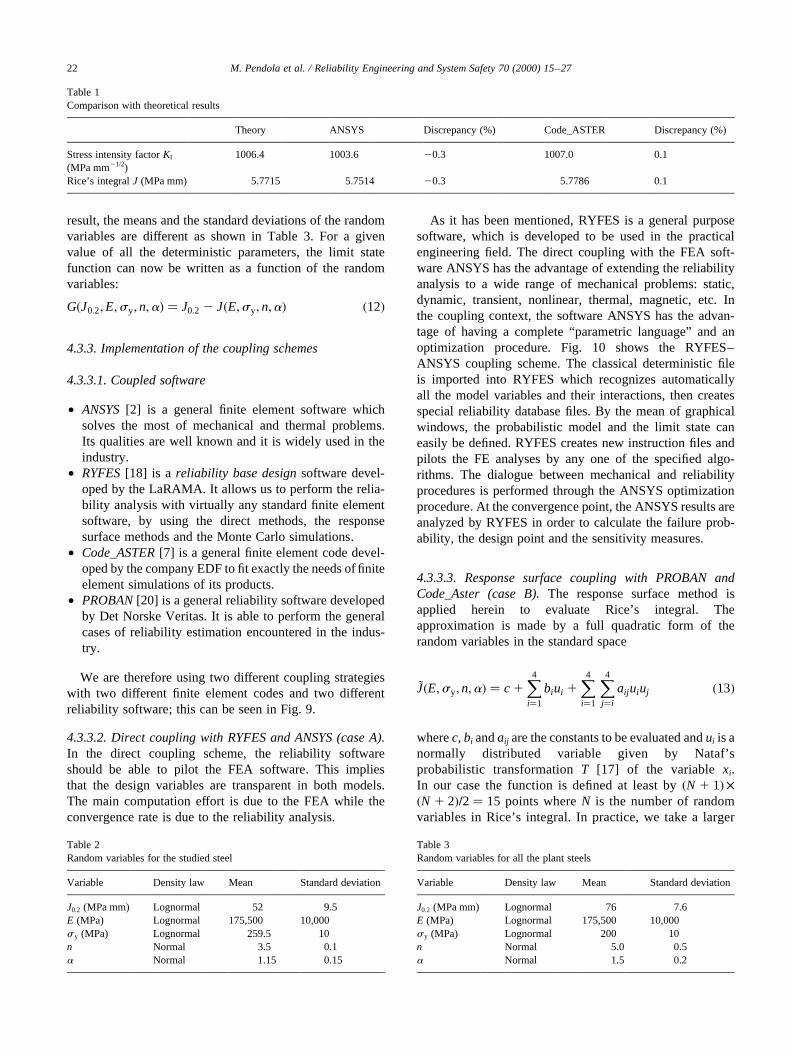
Table 1Comparison with theoretical results

Theory ANSYS Discrepancy (%) Code_ASTER Discrepancy (%)

Stress intensity factorKI

(MPa mm21/2)1006.4 1003.6 20.3 1007.0 0.1

Rice’s integralJ (MPa mm) 5.7715 5.7514 20.3 5.7786 0.1

Table 2Random variables for the studied steel

Variable Density law Mean Standard deviation

J0.2 (MPa mm) Lognormal 52 9.5E (MPa) Lognormal 175,500 10,000s y (MPa) Lognormal 259.5 10n Normal 3.5 0.1a Normal 1.15 0.15

Table 3Random variables for all the plant steels

Variable Density law Mean Standard deviation

J0.2 (MPa mm) Lognormal 76 7.6E (MPa) Lognormal 175,500 10,000s y (MPa) Lognormal 200 10n Normal 5.0 0.5a Normal 1.5 0.2

number r of points and the approximation is obtainedby regression.

4.4. Reliability results

4.4.1. Comparison of direct coupling and QRS resultsFig. 11 shows the evolution of the failure probability of

the pipe versus the applied tensile stress obtained by the twomentioned coupling methods when using the typical steelproperties. It is shown that both methods give the samefailure probability level (in a wide range of probability:10210 up to 1) which allows us to rely on the obtainedresults. This conclusion concerns the results relative to the

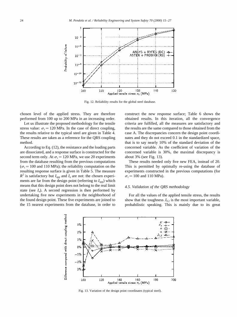
global steel database too (Fig. 12) although the maximaldiscrepancy reaches approximately one decade when theprobability is very small (less than 1029).

Referring to this and knowing the crack length, we candecide whether the repairing of the pipe has to be made in anemergency or if it can wait. Conversely, if an acceptablefailure probability level is decided, the curve shows theallowable load that the structure should support. For exam-ple, an acceptable risk of failure of 1022 corresponds to atensile stress of nearly 150 MPa for the typical steel and atensile stress of 130 MPa for all the other pipes. As a conclu-sion, the pipes made with the typical steel have no restrictiveeffects, i.e. we can load them until 150 MPa without goingover a probability of failure of 1022 but they become lesssafe than for the nominal loading, i.e. around 100 MPa.

In our case, adding the crack length in the parameters ofthe failure probability evolution could for instance, point outan allowable crack length under a certain load. Such resultsare important for the operator to optimize the functioningconditions of the installation with a certain level ofreliability.

Figs. 13 and 14 show that we obtain the same results forthe coordinates of the design point with different couplingmethods and with different finite element software. Themaximum discrepancy concerns the values in distributiontails and for the most important variables (probabilisticallyspeaking).

For each value of the applied tensile stress, the evaluatedfailure probability and the design point coordinates showthat the results are the same. It is therefore proved bycomparison that the results are validated.

4.4.2. Methodology for the QRS coupling schemeFor a given value of the applied stress, the main reliability

results are the failure probability, the design point and theimportance factors (by importance factors we mean thesquared values of the directional cosines in the standardizedspace). The parametric analyses are performed at each


Fig. 9. Coupling implementations for the pipe reliability analysis.

Fig. 10. RYFES–ANSYS coupling scheme.

Fig. 11. Reliability results for the typical steel.

chosen level of the applied stress. They are thereforeperformed from 100 up to 200 MPa in an increasing order.

Let us illustrate the proposed methodology for the tensilestress value:s t� 120 MPa. In the case of direct coupling,the results relative to the typical steel are given in Table 4.These results are taken as a reference for the QRS couplingmethod.

According to Eq. (12), the resistance and the loading partsare dissociated, and a response surface is constructed for thesecond term only. Ats t� 120 MPa, we use 20 experimentsfrom the database resulting from the previous computations(s t� 100 and 110 MPa); the reliability computation on theresulting response surface is given in Table 5. The measureR2 is satisfactory butIapp and Ia are not: the chosen experi-ments are far from the design point (referring toIapp) whichmeans that this design point does not belong to the real limitstate (seeIa). A second regression is then performed byundertaking five new experiments in the neighborhood ofthe found design point. These five experiments are joined tothe 15 nearest experiments from the database, in order to

construct the new response surface; Table 6 shows theobtained results. In this iteration, all the convergencecriteria are fulfilled, all the measures are satisfactory andthe results are the same compared to those obtained from thecase A. The discrepancies concern the design point coordi-nates and they do not exceed 0.1 in the standardized space,that is to say nearly 10% of the standard deviation of theconcerned variable. As the coefficient of variation of theconcerned variable is 30%, the maximal discrepancy isabout 3% (see Fig. 13).

These results needed only five new FEA, instead of 20.This is permitted by optimally re-using the database ofexperiments constructed in the previous computations (fors t� 100 and 110 MPa).

4.5. Validation of the QRS methodology

For all the values of the applied tensile stress, the resultsshow that the toughnessJ0.2 is the most important variable,probabilistic speaking. This is mainly due to its great


Fig. 12. Reliability results for the global steel database.

Fig. 13. Variation of the design point coordinates (typical steel).

coefficient of variation. For example, according to this, thedesigner can concentrate the quality controls on this vari-able which contributes the most in the failure of the struc-ture. The high importance of the toughness implies that onemight put, without serious error, the variables in theJ-inte-gral (i.e.E, s y, n, a ) to their mean values: an evaluation ofthe omission factor [16] would have probably shown thatthis factor is close to 1. In any case, despite the minorimportance of the loading effect for the typical steel, thedesign point coordinates obtained with the response surfaceshow that this method is able to fit accurately the real limitstate in the vicinity of the design point, that is to say in theregion of main interest (see Ref. [26]).

The accuracy of the QRS methodology is confirmed bythe reliability analysis of the global steel database where theloading importance is nearly 80% (Fig. 15). The responsesurface is proven to be suitable for accurate representationof the contribution of theJ-integral variables (i.e.E, s y, n,a ). In this case, the yield stresss y becomes the most impor-tant variable (nearly 60%). Its nonlinear effect given in theRamberg–Osgood law does not perturb the response surfacemethod. The adaptive FEA re-using technique showed avery high performance.

4.6. Efficiency of the QRS method

The response surface method needs more than 15 finite

element analyses to obtain the failure probability for a givenapplied stress (let us take 25 FEA to get accurate results). Incompensation, to perform the complete parametric study asshown in Fig. 11 (computation for 10 values of the appliedtensile stress), about 60 finite element analyses have beenperformed. As it has be shown in the above sections, to


Fig. 14. Variation of the design point coordinates (steel database).

Table 4Reliability results fors t� 120 MPa by direct coupling

Variable Up Xp Importance factors (%)

Pf � 2:01× 1026

b � 4.61J0.2 24.197 23.91 82.5E 21.276 162,930 8.3s y 20.886 250.61 4.0n 20.151 3.48 0.0a 1.098 1.31 5.2

Table 5Reliability results at the first iteration of case B (s t� 120 MPa)


Pf � 1:11× 1026

b � 4.73J0.2 24.30 23.48 82.6E 21.36 162,160 8.3s y 20.93 250.23 4.0n 20.08 3.49 0.0a 1.10 1.32 5.1

MeasuresR2� 98.5%Iapp�223.46Ia� 3%

Table 6Reliability results at the second iteration of case B (s t� 120 MPa)


Pf � 2:07× 1026

b � 4.61J0.2 24.183 23.97 82.5E 21.325 162,480 8.3s y 20.923 250.25 4.0n 20.061 3.49 0.0a 1.047 1.31 5.2

MeasuresR2 < 100%Iapp�25.32Ia� 0.003%

construct the response surface at a given loading level, were-use the finite element computations performed at theprevious stress levels.

For a given applied stress, the direct coupling methodneeds about five iterations which represents 30 finiteelement computations (because the response gradient isevaluated by finite difference technique), that is to sayabout 300 calculus for the whole curve of Fig. 11.

This great computation number can be greatly decreasedby programming the gradient operators in the finite elementsoftware and by making the convergence criteria more flex-ible (leading to less precision). Even if we imagine that thenumber of the direct coupling iteration could be reduced to 2(which is the minimum), the calculation of the probabilitycurve in Fig. 11 requires at least 120 finite element compu-tations, i.e. number of iterations× (1 1 number of randomvariables)× number of tensile stress values.

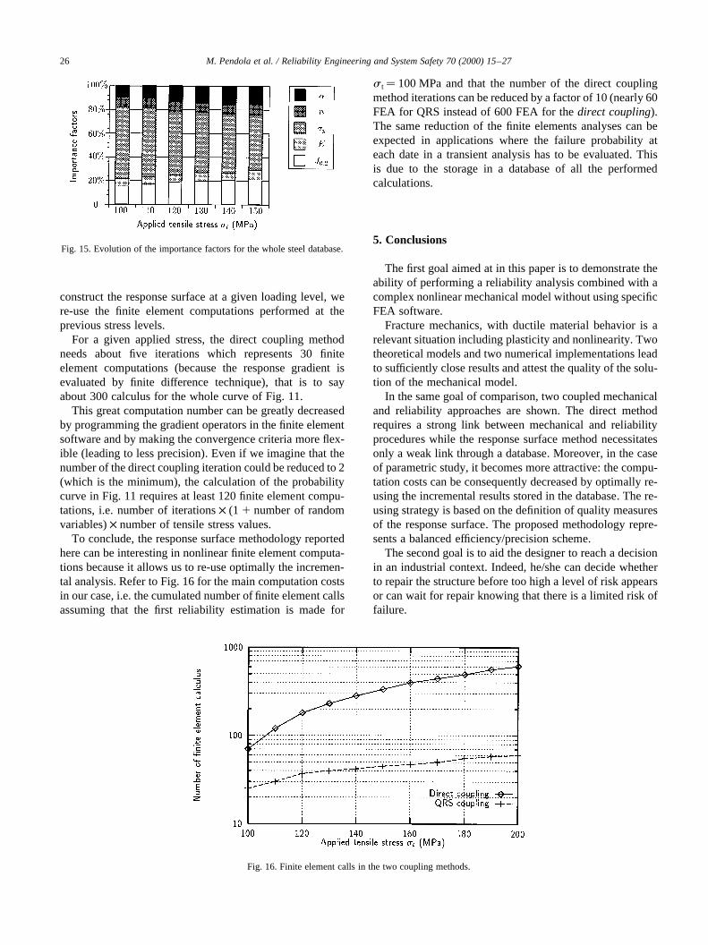
To conclude, the response surface methodology reportedhere can be interesting in nonlinear finite element computa-tions because it allows us to re-use optimally the incremen-tal analysis. Refer to Fig. 16 for the main computation costsin our case, i.e. the cumulated number of finite element callsassuming that the first reliability estimation is made for

s t� 100 MPa and that the number of the direct couplingmethod iterations can be reduced by a factor of 10 (nearly 60FEA for QRS instead of 600 FEA for thedirect coupling).The same reduction of the finite elements analyses can beexpected in applications where the failure probability ateach date in a transient analysis has to be evaluated. Thisis due to the storage in a database of all the performedcalculations.

5. Conclusions

The first goal aimed at in this paper is to demonstrate theability of performing a reliability analysis combined with acomplex nonlinear mechanical model without using specificFEA software.

Fracture mechanics, with ductile material behavior is arelevant situation including plasticity and nonlinearity. Twotheoretical models and two numerical implementations leadto sufficiently close results and attest the quality of the solu-tion of the mechanical model.

In the same goal of comparison, two coupled mechanicaland reliability approaches are shown. The direct methodrequires a strong link between mechanical and reliabilityprocedures while the response surface method necessitatesonly a weak link through a database. Moreover, in the caseof parametric study, it becomes more attractive: the compu-tation costs can be consequently decreased by optimally re-using the incremental results stored in the database. The re-using strategy is based on the definition of quality measuresof the response surface. The proposed methodology repre-sents a balanced efficiency/precision scheme.

The second goal is to aid the designer to reach a decisionin an industrial context. Indeed, he/she can decide whetherto repair the structure before too high a level of risk appearsor can wait for repair knowing that there is a limited risk offailure.


Fig. 15. Evolution of the importance factors for the whole steel database.

Fig. 16. Finite element calls in the two coupling methods.

References

[1] Abdo T, Rackwitz R. A new beta-point algorithm for large time-invariant and time variant reliability problems. Third WG IFIP Work-ing Conference, Berkeley, 1990.

[2] Ansys, Inc. ANSYS 5.5—Finite Element Software, User’s Manual,1999.

[3] ASTM. Standard test method forJIc, a measure of fracture toughness.Annual Book of ASTM Standards, 0301, 1989.

[4] Bucher CG, Bourgund U. A fast and efficient response surfaceapproach for structural reliability problems. Struct Safety1990;7:57–66.

[5] Casciati F, Colombi P. In: Spanos PD, Wu YT, editors. Fatigue life-time prediction for uncertain systems, Berlin: Springer, 1994.

[6] Colombi P, Faravelli L. In: Guedes Soares C, editor. Stochastic finiteelements via response surface: fatigue crack growth problems,Dordrecht: Kluwer Academic, 1997.

[7] DER-EDF. Manuel d’Utilisation et Manuel de Re´ference de Code_A-STER. Electricite´ de France, 1995.

[8] Der Kiureghian A, Liu PL. Structural reliability under incompleteprobability information. J Engng Mech 1986;112(1):85–104.

[9] Devictor N, Marques M, Lemaire M. Adaptative use of responsesurfaces in the reliability computations of mechanical components.In: Guedes Soares C, editor. Advances in safety and reliability, vol. 2.Amsterdam: Elsevier, 1997. p. 1269–77 (ESREL’97, Lisbon 17–20June).

[10] Enevoldsen I, Faber MH, Sørensen JD. Adaptative response surfacetechniques in reliability estimation. In: Schueller GI, Shinozuka M,Yao I, editors. Structural safety and reliability, 1994. p. 1257–64.

[11] Faravelli L. Response surface approach for reliability analysis. JEngng Mech 1989;115(12):2763–81.

[12] Hutchinson JW. Fundamentals of the phenomenological theory ofnonlinear fracture mechanics. J Appl Mech 1983;50:1042–51.

[13] Kim SH, Na SW. Response surface method using vector projectedsampling points. Struct Safety 1997;19(1):3–19.

[14] Krishnaswamy P, Scott P, Rahman S, et al. Fracture behavior of shortcircumferentially surface-cracked pipe. US Nuclear RegulatoryCommission, Washington, DC, September 1995.

[15] Lemaire M. Finite element and reliability: combined methods byresponse surface. In: Frantziskonis GM, editor. Prabamat-21stCentury: probabilities and materials, Dordrecht: Kluwer Academic,1998. p. 317–31.

[16] Madsen HO. Omission sensitivity factors. Struct Safety1988;5(1):35–45.

[17] Madsen HO, Krenk S, Lind NC. Methods of structural safety. Engle-wood Cliffs, NJ: Prentice-Hall, 1986.

[18] Mohamed A, Suau F, Lemaire M. A new tool for reliability baseddesign with ANSYS FEA. ANSYS, Inc., ANSYS Conference andExhibition, Houston, TX, USA, 1996. p. 3.13–3.23.

[19] Muzeau JP, Lemaire M, El-Tawil K. Me´thode fiabiliste des surfacesde reponse quadratiques (srq) et e´valuation des re`glements. Construc-tion Metallique (3), Septembre 1992.

[20] Olesen R. PROBAN User’s Manual. Technical report, Det NorskeVeritas Sesam, 1992.

[21] Pendola M. Couplage me´cano-fiabiliste par surfaces de re´ponse.Application auxtuyauteries droites fissure´es. Master’s thesis,LaRAMA-UniversiteBlaise-Pascal, Clermont-Ferrand, 1997.

[22] Rackwitz R, Fiessler B. Structural reliability under combined randomload sequences. Computer Struct 1978:489–94.

[23] Rahman S, Brust FW, Ghadiali N, Choi YH, Krishnaswamy P,Moberg Brick-stad F, Wilkowski GM. Refinement and evaluationof crack-opening-area analyses for circumferential through-wallcrack in pipes. US Nuclear Regulatory Commission, Washington,DC, April 1995.

[24] Rajashekhar MR, Ellingwood BR. new look at the response surfaceapproach for reliability analysis. Struct Safety 1993;12(3):205–20.

[25] Rice JR. A path independent integral and the approximate analysis ofstrain concentrations by notches and cracks. J Appl Mech 1968:379–86.

[26] Rollot O, Pendola M, Lemaire M, Boutemy I. Reliability indexescalculation of industrial boilers under stochastic thermal process.Proceedings of the 1998 ASME Design Engineering TechnicalConference, September 13–16 1998.

[27] Sih G. Mechanics of fracture. Vols. I–V. Leiden:Noordhoff, 1973–1977.


Documents

Combination of ﬁnite element and reliability methods in