COMBINATION OF GEODETIC NETWORKS

D. B. THOMSON

April 1976

TECHNICAL REPORT NO. 30

PREFACE

In order to make our extensive series of technical reports more readily available, we have scanned the old master copies and produced electronic versions in Portable Document Format. The quality of the images varies depending on the quality of the originals. The images have not been converted to searchable text.

COMBINATION OF GEODETIC NETWORKS

Donald B. Thomson

Department of Surveying Engineering University of New Brunswick

P.O. Box 4400 Fredericton, N.B.

Canada E3B 5A3

April1976 Latest Reprinting February 1994

PREFACE

This report is an unaltered version of the author's

doctoral thesis entitled "A Study of the Combination of Terrestrial

and Satellite Geodetic Networks". A copy of this report was submitted

to the Geodetic Surveys of Canada in partial fulfillment of a Research

Contract.

The thesis advisor and supervisor of the research carried

out was Dr. E. J. Krakiwsky. Acknowledgement of the assistance

rendered by others is given in the ACKNOWLEDGEMENTS.

ABSTRACT

The rigorous combination of terrestrial and satellite

geodetic networks is not easily accomplished. There are many factors

to be considered. The more important are how to deal with terrestrial

networks that are separated into horizontal and vertical components

which are not usually coincident; the relation of each component to

a different datum; and the existence of unmodeled systematic errors

in terrestrial observables. Satellite networks are inherently three­

dimensional and are relatively free of systematic errors. In view of

these facts, and with present practical considerations in mind, four­

teen alternate Mathematical models for the combination of terrestrial

and satellite geodetic networks are investigated, catalogued and

categorized in this report.

To understand the reasoning behind the formulation of the

models presented and the interpretation of the results obtained, some

basic definitions and properties of datums, and satellite and

terrestrial networks are presented.

Based on previous investigations and the author's interpre­

tation of the problem of combining geodetic networks, the models under

study are split into two major groups. The first group treats datum

ii

transformation parameters as known, while the second includes them as

unknowns to be estimated in the combination procedure. Each model is

investigated in terms of its dimensionality, unknown parameters to be

estimated, observables, and the estimation procedure utilized.

The group of three-dimensional models that treat the datum

transformation parameters as unknowns to be estimated are themselves

separated into two parts. The Bursa, Molodensky, and Veis models

contain only one set of rotation parameters each, while the Hotine,

Krakiwsky-Thomson, and Vanicek-Wells models each contain two sets of

unknown rotations. For the combination of terrestrial and satellite

networks, the latter three models represent physical reality.

The models that are not three-dimensional do not take

advantage of the inherent tri-dimensionality of satellite networks.

Thus, when the satellite network data is split into horizontal and

vertical components for combination with terrestrial data, the

covariance between the components is omitted. Even though the use

of two and one-dimensional combination models are required at present

due to the sparseness of adequate terrestrial data and the need for

the solution of practical problems, it is not recommended for the

future.

The Bursa model is recommended for the combination of two

or more satellite networks. However, when combining terrestrial and

satellite networks, when datum transformation parameters are unknown,

none of the Bursa, Molodensky, or Veis models are adequate. In this

case, the Hotine or Krakiwsky-Thomson model which parameterize the

lower order systematic errors in the terrestrial network, should be

iii

used. To combine several terrestrial datums and one satellite

datum and determine the orientation of these with respect to the

Average Terrestrial system, the Vanicek-Wells model should be used.

A combination of the Krakiwsky-Thomson and Vanicek-Wells

models is seen to be the best, from a theoretical point of view, for

the combination of a satellite and several terrestrial networks. Such

a solution will yield the datum transformation parameters between each

of the datums involved, the orientation of each datum with respect to

the Average Terrestrial coordinate system, and parameters representing

the overall systematic orientation and scale errors of each terrestrial

network.

No substantiative conclusions could be given based on the

numerical testing carried out. A sparseness of adequate data

prevented this. The numerical testing has not been wasted, however.

The type and quality of data required for several models has been

demonstrated. Further, the available data was utilized to substan­

tiate the fact that the proposed solution of the Krakiwsky-Thomson

model is possible.

iv

TABLE OF CONTENTS Page

ABSTRACT . . . . . . . . . . . . . . . . . . . . . . . . . . . . . . . . . . . . • . . . . . . . . . . . . . . . . . i i

LIST OF FIGURES . • . . . . . . . . . . . . . . . . • . . . . . . . . . . • . . . • • . . . . . • . . . . . . viii

LIST OF TABLES . . . . . . . . . . . . . . . . . . . . . . . . . . . . . . . . . . . . . . . . . . . . . . . . ix

ACKNOWLEDGEMENTS . . . . . . . . . . . . . . . . . . . . . . . . . . . . . . . . . . . . . . . . . . . . . . x 1

0. INTRODUCTION . . . . . • . . . . . . . . . . . . . . . . . . . . . . . . . . . . . . . . . . . . . . . . . l

0. 1 Background . . . . . . . . • . . . . . . . . . . . . . . . . . . . . . . . . . . . . . . . . . . . . l 0.2 Objective and Methodology . . . . . . . . . . . . . . . . . . . . . . . . . . . . . . 3 0.3 Scope .. .. .. .... ... .. ....... ...... ... ... .. .. .•.. ........ 5 0. 4 Contributions . . . . . . . . . . . . . . . . . . . . . . . . . • . . . . . . . . . . . . . . . . 7

SECTION I - GEODETIC DATUMS, GEODETIC NETWORKS, AND COMBINATION PROCEDURES

1. GEODETIC DATUMS ............................ . 9

l.l Classical Geodetic Datums . . . . . . . . . . . . . . . . . . . . . . . . . . . . . . 10 1.2 Ellipsoidal Geodetic Coordinates, Orthometric Height,

and the Geodetic Coordinate System ..................... 14 1.3 Positioning and Orienting of a Terrestrial Horizontal

Network Datum . . . . . . . . . . . . . . . . . . . . . . . . . . . . . . . . . . . . . . . . . . 16 1.4 Contemporary Concepts 23

2. TERRESTRIAL AND SATELLITE GEODETIC NETWORKS ................ 28

2.1 Terrestrial Geodetic Networks . . . . . . . . . . . . . . . . . . . . . . . . . . 29 2.1.1 Horizontal Geodetic Networks ..................... 30 2 .1. 2 Vertical Geodetic Networks . . • . . . . . . . . . . . . . . . . . . . . 34 2.1.3 Three-Dimensional Terrestrial Geodetic Networks .. 36

2. 2 Satellite Geodetic Networks . . . . . . . . . . . . . . . . . . . . . . . . . . . . 39 2.2.1 North American Densification of the World

Geometric Satellite Triangulation (BC-4) Network . 42 2.2.2 North American Doppler Networks .................. 46

3. GENERAL CONCEPTS REGARDING THE COMBINATION OF GEODETIC NETWORKS . . . . . . . . . . . . . . . . . . . • . . . . . . . . . . . . . . . . . . . . . . . . . . . . . . . 50

3 . 1 Rationale . . . . . . . . • . . . . . • . . . . . . . . . . . . . . . . . . . . . . . . . . . . . . . 52 3.2 Classification of Mathematical Models .................. 54

v

SECTION II - COMBINATION PROCEDURES WHEN DATUM TRANSFORMATION PARAMETERS ARE KNOWN

4. THREE-DIMENSIONAL MODELS

4.1 A Parameterization of Scale and Orientation Errors in

Page

60

a Terrestrial Network • . . • • • . . . . . • . . . . . . . . . . . • . . . . . . . • . • 61 4.2 S<J.tellite Coordinates as Weighted Parameters ••••.•••.•• 66 4.3 Satellite Coordinate Differences as Observables ...•.... 70 4.4 Computed Spatial Distances, Azimuths, and Vertical

Angles as Observables . . . . • . . . . . . . . . . . . . . . . • . . . . . . . . . . • . 71

5. TWO-DIMENSIONAL MODELS . . . . . • • . . • . • . . . • . • . • . . . • . • . • • . • • . • . . • 74

5.1 Satellite Coordinates as Weighted Parameters ..•.•.•.... 75 5.2 Satellite Coordinate Differences as Observables .•.•••.. 78 5.3 Computed Distances and Azimuths as Observables ········- 79

6. ONE-DIMENSIONAL MODELS 84

6.1 Vertical Networks and Geoidal Heights •...•••••••••••••. 85

SECTION III - COMBINATION PROCEDURES WHEN DATUM TRANSFORMATION PARAMETERS ARE UNKNOWN

7. STANDARD MODELS . . . . • . . . • • . . . . . . . . . . . . . . . . . . . . . . . . . . . • . . . . . . 89

7. 1 Bursa . • . . • . • . . . . • . . . . . . . . . . . . . . . . . . . . . . • . . . • . . . . . . . . . . . 90 7. 2 Molodensky . . . . . . . . . . . . . • . . . . . . . . . . . . . . . • . . . . . . . . . . . . . . . 94 7. 3 Veis . . . . • . . . • . . • . • . . . . . • . • . . . . . • • . . . . . • . • . . • . • • . . • . • . • . 97 7.4 Comparison of Bursa, Molodensky and Veis Models .••••.•. 101

8 . RECENT MODELS • . • • . • . . • . . . • • . . • • . . • . . . . . . . . . . • . . • . . . . • . • . . . . 104

8.1 Hotine ...................................•.........•... 105 8. 2 Krakiwsky-Thomson . . . • . . . . . • . . . . . . . . . . . . . . . . . . • . • . . . • . . . 111 8.3 Vanicek-Wells ...............•..............•...•.•...•• 122 8.4 Comparison of the Hotine, Krakiwsky-Thomson, and

Vanicek-Wells Models .•.••....•••..•••••....•.••.•.••••. 124 8.5 Comparison of Hotine, Krakiwsky-Thomson, Vanicek-Wells

Models with those of Bursa, Molodensky, and Veis ..•.••• 126

9. SUMMARY . • • • • . • . . • • . . • . . . • . • . . • . . . . . . . • . • . . . • . . • • . . • . • . . • • • . 129

SECTION IV - TEST RESULTS

10. MODELS FOR WHICH DATUM TRANSFORMATION PARAMETERS ARE KNOWN . 138

10.1 Satellite Coordinates as tveighted Parameters •.•••.•••. 139 10.2 Computation of Satellite Network Distances, Azimuths

and Associated Variance-Covariance Matrix ••••.••••.•.. 151

Page

11. STANDARD THREE-DIMENSIONAL MODELS - UNKNOWN DATUM TRANSFORMATION PARAMETERS • . • • • • • • . . . • . . . . • . . • • . . • . . . . • • . . • 158

11.1 Bursa Model • • . . . . . . . . . . . . • • • . • . • • . . . . . . • • . . • . • . . . . • . • 158 11.2 VoiH and Moloden:;ky Modt'ls .•..........•.•..•••••••••• 176 11.3 Compar-ison of Hcsull.s .... .•..••... .•....•.•....•.••.• 179

12. RECENT THREE-DIMENSIONAL MODELS - UNKNOWN DATUM TRANS-FORMATION PARAMETERS . . . • . . . . . • • • . • . • . . . . . . • . • . . . • • • . • • . . • • 181

12 .1 Krakiwsky-Thomson Mo.de1 . . . • . . . . • . . . . . . . • • . . . . . . . . • • • . 182

SECTION V - CONCLUSIONS AND RECOMMENDATIONS

13. CONCLUSIONS AND RECOMMENDATIONS .......... .....•....••...•. 187

REFERENCES . • . . • . . . • . . . . . • . . . . . • . • . . . . . . • . . . . . . . . • . • . • • • . • • . • • . 192

vii

Figure 1-l

Figure l-2

Figure l-3

Figure l-4

Figure 2-l

Figure 2-2

Figure 3-l

Figure 4-l

Figure 7-l

Figure 7-2

Figure 7-3

Figure 8-l

Figure 8-2

Figure 8-3

Figure 8-4

Figure 10-l

Figure 10-2

Figure ll-1

Figure ll-2

LIST OF FIGURES

The Reference Ellipsoid, Geodetic Latitude and Longitude, and the Geodetic Coordinate System

Reference Surfaces and Heights

The Average Terrestrial Coordinte System

Relationship of the Average Terrestrial and Geodetic Coordinate Systems

North American Densification of the World Geometric Satellite Triangulation {BC-4) Network

Page

11

13

l7

25

43

1974 Status of Canadian Doppler Network 47

Combination of Geodetic Networks 51

A Parameterization of Terrestrial Network Systematic Errors 63

Bursa Model 91

Molodensky Model 95

Veis Model 98

Hotine Model 107

Krakiwsky-Thomson Mode}. 112

Estimation Procedure for the Krakiwsky-Thomson Model 115

Vanicek-Wells Model 123

Doppler Coordinates as Weighted Parameters 111 a Horizontal Network Adjustment 140

Displacement Vectors: Adjustment with Terrestrial Observables Only Minus Adjustment with Doppler Coordinates as Weighted Parameters 146

Five Doppler Tracking 3tations in Atlantic Canada 160

Twenty-one Doppler Tracking Stations in the United States of America 171

viii

Table 3-1

Table 9-1

Table 9-2

Table 9-3

Table 10-1

Table 10-2

Table 10-3

Table 10-4

Table 10-5

Table 10-6

Table 10-7

Table 10-8

Table 10-9

Table 11-1

Table 11-2

Table 11-3

LIST OF TABLES

Classification of Mathematical Models

Datum Transformation Parameters Known - General Characteristics of the Combination Models Studied

Datum Transformation Parameters Unknown -General Characteristics of the Combination Models Studied

summary of· the Uses of the Three-Dimensional (Unknown Datum Transformation Parameters) Models Studied

Doppler Coordinates Used as Weighted Parameters

Results of Least-Squares Adjustment Using Terrestrial Observables

Results of Least-Squares Adjustment Using Terrestrial Observables and Doppler Coordinates as Weighted Parameters

Effects on Doppler Coordinates as a Result of Combination with Terrestrial Data

Results of Least-Squares Adjustment Using Terrestrial Observables and Doppler Coordinates as Weighted Parameters (Diagonal Elements only of Px)

Coordinates of Doppler Tracking Stations

Rigorously Computed Doppler Network Ellipsoidal Distances and Azimuths

Doppler Network Spatial Distances and Azimuths Reduced to the Reference Ellipsoid

Differences in Distances, Azimuths, and Associated Standard Deviations

Combination of Two Sets of Doppler Coordinates

Bursa Model Tests. Combination of Two Sets of Doppler Data

Adjusted Coordinates as a Result of the Combination of Two Sets of Doppler Coordinates

Page

56

132

135

136

141

144

145

147

150

153

154

155

156

161

164

165

Table 11-4

Table 11-5

Table 11-6

Table 11-7

Table 12-l

LIST OF TABLES (Cont'd)

Doppler Coordinates Coincident with Transcontinental Traverse Points

U.S.A. Transcontinental Traverse Coordinates

Bursa Model Tests: Combination of a Doppler and a Terrestrial Network

Veis and Molodensky Model Tests: Combination of a Terrestrial and a Doppler Network

Test Results of the Krakiwsky-Thomson Model

X

Page

168

170

174

178

184

ACKNOWLEDGEMENTS

This work was partially funded by the Geodetic Survey of

Canada. They also provided much of the data utilized for numerical

testing. Their interest in the topic and assistance given were very

helpful.

The National Research Council of Canada is thanked for the

financial support given in the form of three consecutive Post Graduate

Scholarships.

My sincere thanks go to my thesis advisor, and research

supervisor, Dr. E.J. Krakiwsky. The many hours spent with him

discussing this work were invaluable. His interest in the topic

never faltered, for which he has my gratitude.

The help given by Dr. P. Vanicek is acknowledged. Discussions

with him on this and related topics were always enlightening.

I would like to acknowledge the assistance given by my

fellow graduate students in the Department of Surveying Engineering.

Those to whom I owe special thanks are Drs. D.E. Wells and C.L. Merry,

and Messrs. M.M. Nassar and C.A. Chamberlain. Working and studying

with them was a pleasure and an education.

The help given by Messrs. J. Kouba of the Geodetic Survey of

xi

Canada and A. Pope of the U.S. National Geodetic Survey is appreciated.

Their comments on earlier papers and reports on this topic have been

extremely helpful.

Messrs. w. Strange and B.K. Meade of the U.S. National

Geodetic Survey are thanked for contributing some of the data used

for numerical testing.

For their help in preparing the manuscript, I would like

to thank Mrs. D. Smith for her excellent typing and Mrs. D. Jordan

for her excellent drafting.

I dedicate this work to Allison. There are no words that

can adequately express my gratutude to her. Her patience, under­

standing, and support have been immeasurable. She has sacrificed

much and I shall be forever grateful.

xii

0. INTRODUCTION

0.1 Background

In the broad spectrum of activities covered by geodesy, one

of the primary tasks is the establishment of geodetic networks.

These networks, which may be of a local or regional nature, or even

of global extent, have a variety of uses in the realms of both scien­

tific and applied geodesy. The establishment of geodetic networks

and the datums to which they are referred are massive tasks. Using

only classical terrestrial observables, the problems encountered are

numerous. The 1927 North American Datum and associated horizontal

networks are an example of the results obtained using limited

terrestrial observables and limited computing facilities. Three­

dimensional satellite geodetic networks are a new tool that can be

used by geodesists in the establishment of terrestrial geodetic

datums and networks.

The notion of combining terrestrial and satellite geodetic

networks, for the purpose of solving some of the problems associated

with terrestrial datums and networks, began with the establishment

of the first geodetic satellite networks. Some of the first math­

ematical models for the combination process were applied in the

1

2

investigation of the position and orientation of the terrestrial net­

work datum with respect to that of the satellite network [Bursa, 1962;

Bursa, 1967; Lambeck, 1971]. In many instances combination models

were derived utilized in conjunction with other geodetic invest­

igations [Veis, 1960; Molodensky et al, 1962; Badekas, 1969]. As

the accuracy and density of satellite determined geodetic networks

increased, the mathematical models used to combine them with their

terrestrial counterparts have become more varied and sophisticated.

For example, there are those that parameterize both the position

and orientation of the terrestrial network datum with respect to

the satellite network datum and the unknown systematic errors in

the terrestrial networks [Hotine, 1969; Krakiwsky and Thomson, 1974]. ·

Another is useful in the combination of several terrestrial networks

with one satellite network in which the orientation of their datums

with respect to the Average Terrestrial coordinate system is deter­

mined [Wells and Vanicek, 1975]. In the future, as satellite

methods yield coordinates of centimetre accuracy, it is envisaged

that rigorously combined satellite and terrestrial networks, along

with the results of new technology such as.VLBI, will be important

tools in the establishment of three-dimensional, time-varying,

geodetic coordinates that are necessary for geophysical and

geodynamic purposes.

3

0.2 Objective and Methodology

What mathematical model should be used for the rigorous

combination of satellite and terrestrial geodetic networks? There

is no simple answer to this. There are many models available and

the use of one or another of them is dependent on several factors,

not the least of which are the ultimate objectives of the user.

To be able to choose a particular model to solve a certain problem,

the user should be aware of the implications of the choice. The

objective of this study is to outline how to choose an appropriate

mathematical model for the combination of satellite and terrestrial

geodetic networks and why certain models should be used in different

circumstances.

The main method used in this report is to catalogue, categorize,

analyse, and test several models. This approach of covering the

broad spectrum of the combination of satellite and terrestrial

geodetic networks as opposed to intense investigation of one or two

mathematical models was arrived at because of certain circumstances.

After some preliminary research, it was found that various opinions

existed regarding the foundation, formulation, use, and interpret-

ation of several models. These points required clarification.

Further, it was found that there was insufficient data to adequately

investigate any one model in which the final analysis and conclusions

would be based on the solution of an actual combination of some

existing satellite and terrestrial networks. These facts lead to

the present format of the stud~

4

To accomplish the stated objective using the aforementioned

methodology, several tasks have to be completed. One of these is

to substantiate why satellite geodetic networks should be combined

with their terrestrial counterparts and to set out the concepts

upon which the combination mathematical models are based. This

involves the definition, in terms of current geodetic thought, of

geodetic datums and the parameters that are used to define them.

Chapter 1 is devoted to this. In Chaper 2, geodetic networks

(terrestrial and satellite), their relationships with their respec­

tive datums and their inherent properties, are described. Section

I is concluded by Chapter 3 in which the rationale for combining

geodetic networks is given, along with a classification and listing

of several models.

Another task is to examine several combination models in

detail in order that a logical scheme of categorization can be

produced. This involves the study of a priori assumptions, dimen­

sionalities of models, treatment of unknown parameters such as

datum transformation elements and systematic errors in the

terrestrial networks,and the interpretation of results. These

are the underlying considerations in Section II and Section III.

In the former, three separate chapters deal with the combination of

terrestrial and satellite networks when the transformation param­

eters between their respective datums are considered known, while

in the latter, two chapters deal with models in which datum trans­

formation parameters are treated as unknowns to be solved for in

5

the combination procedure. Section IV, TEST RESULTS, presents some

numerical tests using data from North American terrestrial and

satellite geodetic networks.

The fulfillment of the objective of this study is attained

in Chapter 9. Here, the various models are presented in three tables.

These outline the proper application and interpretation of the various

models considered for the combination of terrestrial and satellite

geodetic networks.

0.3 Scope

Several events in geodesy prompted this research. By the

late 1960's, the coordinates of terrestrial points were being

determined with 5 m (1 a) accuracy using satellite methods. Today,

1 m standard deviations are commonplace and decimetre accuracy is

predicted for the near future. The problems inherent in the North

American terrestrial geodetic network and the decision to redefine

it was another contributing factor. It was recognized that the

three-dimensional satellite networks could contribute invaluably

in the positioning and orientating of a new geodetic datum and in

the definition of a more accurate and homogeneous terrestrial

geodetic network. Finally, there was the fact that.the geodetic

record, of which geodetic networks arc an integral part, was being

utilized more frequently in the solution of related scientific and

6

practical problems. In order that this contribution be more

valuable, geodesists must move towards the so-called four­

dimensional system - a rigorous system of three-dimensional,

time-varying coordinates.

As explained previously, the aim of this study is to

cover the broad spectrum of the combination of geodetic networks.

However, it was carried out within a certain framework. To have

immediate practical value it was decided to devote a major portion

of the study to combination models in which the ultimate objective

was the positioning and orienting of a geodetic datum and the

de~tknof a more accurate and homogeneous terrestrial geodetic

network. Further, models in which presently available geodetic

network data could be realistically used were given priority. Due

to the inherently three-dimensional nature of satellite networks

and geodetic datums, a concentrated effort was made on the three­

dimensional models.

The aforementioned constraints have not inhibited this

study. Combination models and procedures utilized in other studies

are included. Several new models and variations of older ones are

presented. Detailed explanations of previously used models, lacking

in some studies, are given. The estimation techniques required

to obtain solutions for all models are explained. Test results,

and their interpretation, are given for several solutions.

7

0.4 Contributions

This study has resulted in several contributions to the

subject of the coru1ination of satellite and terrestrial geodetic

networks. Nine of these, considered to be the most significant

are:

(i) a comprehensive description of classical and contemporary geodetic

network datums and their positioning and orienting in the

earth body;

(ii) an enumeration of the sources of systematic errors in the

observables used to define terrestrial networks;

(iii) the discovery of some shortcomings in several of the presently

used combination models;

(iv) an explanation of the differences amongst presently used three­

dimensional combination models;

(v) an alternative derivation of the Hotine combination model;

(vi) the development of a new model for the combination of

terrestrial and satellite networks in which the lower order

effects of systematic errors in the terrestrial network are

modeled by three rotations and a scale difference parameter;

(vii) the generation of numerical results from the solution of

several models using the same data and an explanation of the

differences obtained;

(viii) the cataloguing and categorizing of fourteen models for the

combination of terrestrial and satellite geodetic networks;

(ix) the construction of tables that can be used to choose a correct

model, under a given set of conditions, for the combination of

satellite and terrestrial geodetic networks.

8

SECTION I

GEODETIC DATUMS, GEODETIC NETWORKS,

AND COMBINATION PROCEDURES

l. GEODETIC DATUMS

The word'aatum' is defined as "a real or assumed thing used

as a basis for calculations" [Webster's, 1951]. The definition of

a geodetic datum is then that "thing" to which geodetic computations

are referred. In the past there has been much confusion regarding

geodetic datums, particularly with regards to their relationship

with geodetic networks [e.g. Jones, 1973]. This was brought on,

in part, by the mixing of the datum with its position and orientation

within the earth body, and with the mixing of the networks themselves

and the datum to which they were referred.

The aim here is to first define the geodetic datums presently

used in North America for terrestrial geodetic networks (horizontal

and vertical), to point out the relationships between them, and to

show the connection between present geodetic coordinates and those of

a unified three-dimensional coordinate system. Second, the classical

means of positioning and orienting a horizontal geodetic

datum in the earth body is presented. The classical parameters are

related to those of contemporary three dimensional methods. The

vertical datum, and its position, is of no less importance. However,

due to the complexities of the problems related to it [e.g. Bomford,

1971], a detailed discussion was deemed beyond the scope of this work.

9

10

Finally, the modern concept of a datum required for three

dimensional geodesy is presented. The means of establishing datums

for a satellite networks are given, with reference to two specific

examples. The position and orientation of the two datums with respect

to each other are discussed in detail.

1.1 Classical Geodetic Datums

During the late seventeenth and early eighteenth centuries,

after having been considered in the past a plane, a convex disk, and

a sphere, the earth was determined to be ellipsoidal in shape. Further

work in the nineteenth and early twentieth centuries by mathematicians

and geodesists showed that the earth's shape is best represented by one

of its equipotential surfaces, the geoid.

The historical developments in the determination of the size

and shape of the earth, and numerous other physical problems, have l.ed

to the traditional splitting of the triplet of coordinates used to

describe the positions of terrain points into horizontal and vertical

components. Further, due to the inherent differences between the

respective terrestrial observables used in the different mathematical

models for horizontal and vertical networks, two separate geodetic

datums must be defined.

The geodetic datum used for classical horizontal terrestrial

networks is a rotational ellipsoid whose size and shape are traditionally

given by the lengths of its semi-major and semi-minor axes, a and b

11

f =(a-b)/a e, =(a,- b,)/a,

Figure 1-1

The Reference Ellipsoid, Geodetic latitude and longitude,

and the Geodetic Coordinate System

12

respectively (Figure 1-1) or its semi-major axis and flattening, f.

Horizontal network computations are carried out on the surface of

this reference ellipsoid. Its size and shape, and position in the

earth body is generally such that it is a "best fitting" ellipsoid

which approximates the geoid most closely. This may refer to the

whole earth or a particular region of it [Heiskanen and Moritz, 1967].

The determination of the dimensions of the reference ellipsoid is a

complex problem in its own right and is not covered in this report.

For this datum to be used for terrestrial network computa­

tions, its position and orientation with respect to some earth fixed

coordinate system must be given. This may be accomplished via some

observations and adherence to certain conditions at a terrestrial

network initial point (1.3). Thus, a classical horizontal geodetic

network datum is completely defined by the size and shape of the

reference ellipsoid and its position and orientation.

The geodetic datum used for vertical networks in North America

is nominally the geoid. The geoid is defined as that equipotential

surface of the earth which "most nearly coincides with the undisturbed

mean sea level" [Mueller and Rockie, 1966]. The delimitation of the

geoid, as a base for vertical networks, is resolved via the determin­

ation of mean sea level at tide-gauge stations [Bamford, 1971; Ku, 1970;

Lennon, 1974]

The distance between the reference ellipsoid and geoid at

any point, the geoidal height N (Figure 1-2), is the "connecting

link" between classical horizontal and vertical geodetic network

13

ELLIPSOIDAL NORMAL

PLUMBLINE \

\ -

Figure 1-2

-----

Reference Surfaces and Heights

LOCAL EQUIPOTENTIAL

SURFACE

TERRAIN

14

coordinates. That is, to express the position of a terrain point

relative to one datum, the aforementioned quantity must be known.

In the next chapter (1.2), the use of the geoidal height in relating

ellipsoidal geodetic coordinates and orthometric height to Cartesian

coordinates is given.

1.2 Ellipsoidal Geodetic Coordinates, Orthometric Height, and the

Geodetic Coordinate System

The relationships amongst ~lassical"geodetic coordinates,

and between them and Cartesian coordinates are important to the dis-

cussions of the positioning and orienting of a classical horizontal

network datum and the relationship of this with three-dimensional

geodetic concepts.

The horizontal position of a terrain point i is given on the

surface of the reference ellipsoid as a set of curvilinear coordinates,

the geodetic latitude (~.) and longitude (!...) [Krakiwsky and Wells, ~ ~

1971] (Figure 1-l). With respect to the Geodetic Coordinate system, the

point can be expressed as a triplet of Cartesian coordinates (x~, y~, z~) ~ ~ ~

in terms of the ellipsoid curvilinear coordinates by [Heiskanen and

Moritz, 1967]

X~ N* cos ~i cos t..i ~ ~

y~ N~ cos ~i sin !... (1-l) ~ ~ ~

z~ N~ 2

sin (1-e ) ~i ~ ~

15

h * · h · · 1 d" f and e 2 1."s the were N. l.S t e pr1.me·vert1.ca ra 1.us o curvature l.

square of the first eccentricity of the ellipsoid.

The vertical coordinate of a terrain point is given by its I

orthometric height, H [e.g. Vanicek, 1972]. In order to relate this

quantity to the horizontal network datum, the geoidal height, N,

must be known. The two quantities are added together to yield the

ellipsoidal height, h (Figure 1-2). This simple addition procedure

neglects the curvature of the actual plumbline and introduces an

error of less than one millimetre in the ellipsoidal height [Heiskanen

and Moritz, 1967].

The triplet ($., A., h.) describes the position of a terrain l. l. l.

point with respect to one datum. In terms of Cartesian coordinates,

one obtains [Heiskanen and Moritz, 1967]

X. (N'!'+h.) cos $i cos A. l. l. l l

yi = (N~+h.) cos $i sin A. (1-2) l l l.

2 sin z. (N~ (1 -e ) +h.) $.

l. l. l. l.

The Cartesian system to which the triplet (x., y., z.) refers l l l

is called the Geodetic coordinate system (Figure 1-1) . It is a right-

handed coordinate system whose origin is coincident with the origin

of the reference ellipsoid. The ZGaxis is directed along the minor

axis of the ellipsoid, and the XGZG plane is in the plane of the

reference geodetic longitude. The YGZG plane is 90° east of the

XGZG plane, and the XGYG plane is coincident with the equatorial plane

of the ellipsoid. The orientation and position of this system is

discussed in 1.3.

16

It is easily seen that via the geoidal height N, and

equation(l-2),one has the relationships between coordinates expressed

on classical datums (~., A., H.}, and those expressed in terms of a 1 1 1

three dimensional coordinate system (~., A., h1.)or (x., y., z.). The 1 1 1 1 1

latter are used extensively in this report in a contemporary and

clear definition of a geodetic datum (1.4) and the formulation of

several mathematical models for the combination of terrestrial and

satellite geodetic networks (Section III).

1.3 Positioning and Orienting of a Terrestrial Horizontal Network

Datum

A body in three-dimensional space has six degrees of

freedom with respect to some fixed reference. An ellipsoid of

rotation, used as a terrestrial horizontal network datum, is located

in the earth body by six parameters with respect to some physical

properties of the earth represented by the Average Terrestrial (AT)

coordinate system (Figure 1-3). The Average Terrestrial system,

conventionally right handed, is defined as having its origin at the

earth's centre of gravity, its third (ZAT) axis oriented towards the

Conventional International Origin (CIO) defined by the International

Polar Motion Service, and its first (X~) axis oriented towards the

Greenwich Mean Astronomical Meridian as defined by the Bureau Inter-

national de l'Heure [e.g. Mueller, 1969]. The condition to be

fulfilled when positioning and orienting the reference ellipsoid is

Figure 1-3

17

CIO

EARTH'S CENTRE

OF GRAVITY

The Average Terrestrial Coordinate System

18

that its axes (Geodetic Coordinate system) be parallel with those

of the earth fixed system (Average Terrestrial system). The fulfill­

ment of this condition is convenient since it tends to simplify

several geodetic equations.

Before proceeding further with the accepted procedure of

positioning and orienting a horizontal terrestrial network reference

ellipsoid, it is necessary to distinguish between geodetic and

geocentric datums. Strictly speaking, a geocentric datum is one whose

origin is coincident with the earth's centre of gravity, and whose

third (Z) axis is coincident with the earth's polar axis of inertia

[e.g. Vanicek, 1975). Such a system can be attained by developing

a set of data such as gravity anomalies, geoidal heights, or deflec­

tions of the vertical, into an infinite series of spherical harmonics

and dropping out the first degree terms [Heiskanen and Moritz, 1967].

Another possibility lies in the use of dynamic satellite geodetic

observations in the establishment of satellite geodetic networks

[Anderle and Tanenbaum, 1974].

Ideally, three translation components and three rotations are

the simplest elements with which to express the position and orienta­

tion of the reference ellipsoid with respect to the Average Terrestrial

coordinate system (1.4). The traditional approach does not do this

directly. First a terrestrial point is chosen and designated as

the network "initial point" (k). At this point, a set of computed

(via terrestrial geodetic observables) and defined quantities are

combined to yield the required six orienting and positioning

parameters.

19

Using astronomical observations, one determines the astra-

nomic latitude (~k) and longitude (Ak) of the initial point, and

the astronomic azimuth of at least one emanating line (~i). The

standard deviations of these quantities will be of the order 0.1 to

0.3.arc seconds for ~k and Ak and 0.2 to 0.4 arc seconds for Aki

[Mueller, 1969]. The orthornetric height of the initial point,~·

can be determined via geodetic leveling. Its standard deviation,

o , will be a function of several factors affecting geodetic levelling. Hk

For example, using a recommended formula for approximating standard

deviations of levelling network points in North America (E = 1.8 K2/ 3

where K. is the distance from the reference stations (s) * in krn) (NASA, 1973],

the uncertainty of the orthometric height at Meade's Ranch, Kansas

(the initial point of the present North American geodetic networks)

can be estimated to be 0.2 m to 0.3 m. Finally, one is able to

measure the zenith distance (Zk.) in the Local Astronomic coordinate . ~

system [e.g. Krakiwsky and Wells, 1971] on any emanating line with a

minimum standard deviation of the order of 1 arc second [Heiskanen

and Moritz, 1967]. The observed values are used in the positioning

and orienting of the network datum.

The quantities that are required in order to start a

terrestrial geodetic network are the geodetic coordinates of the

initial point (~k' Ak' ~),and the geodetic azimuths (aki) and

zenith distances<zk.> of two emanating lines. Note that the deter­~

mination of the above quantities must be carried out in such a way

as to adhere to the condition of parallelity of axes. Further, it

may be required that the ellipsoid be "best-fitting" in terms of

* Mareograph Station(s)

20

geoid-ellipsoid separation over a certain region. The latter problem

is not considered here.

One approach to datum establishment is to assign some

"errorless" geodetic coordinates to the initial point (cr = cr 4>k '\

such that the differences (¢k - ~k) and (Ak - Ak) are sufficiently

sma11 in order that their second powers can be neglected [Bamford,

1971; Heiskanen and Moritz, 1967; Vanicek and Wells, 1974]. As a

consequence the components of the astrogeodetic deflections of the

vertical and geoidal height at the initial point are expressed by

[Heiskanen and Moritz, 1967]

(1-3)

(1-4)

Nk = hk - H k . (1-5)

These expressions are valid if the conditions for parallelity of

axes, expressed via [Hotine, 1969; Vanicek and Wells, 1974]

zki = Zki + (Ak-Ak)cos ~k sin ~i + (¢k-4>k) cos Aki' (1-6)

aki = ~i- (Ak-Ak)sin ~k- [(~k-~k)sin ~i- (~-Ak)cos Aki cos ~kJ cot zki

(1-7)

are fulfilled.

Using this approach, the values of sk' nk' Nk, zki' and

aki each have standard deviations as a result of error propagation in

the respective equations. This implies that while the origin of the

ellipsoid is fixed in space via the assignei geodetic coordinates,

the orientation of its axes is not. Hence, due to errors in the

21

geodetic observations at the initial point, the axes of the ellipsoid

may not be parallel with those of the Average Terrestrial coordinate

system.

An alternative procedure is to define the values of the

deflections of the vertical (~k' nk) and geoidal height (Nk) at the

terrestrial initial point [Heiskanen and Moritz, 1967] (o~ k

a = 0). In this case, the initial point geodetic coordinates will Nk

have some standard deviations as a result of error propagation in

(l-3)through ~-~. and zki and aki as a result of error propagation in

U-6)and Q-~ respectively. Again, the uncertainties are due to the

errors in the original geodetic measurements used

to determine ~k' Ak, ~i' Hk and zki. The result again is the possible

misalignment of the ellipsoidal axeswith those of the Average

Terrestrial coordinate system. A further complication of this

approach is that the geodetic coordinates of the initial point can

not be considered as fixed quantities since they do have some

uncertainty.

The six parameters that are traditionally chosen to rep-

resent the position and orientation of the reference ellipsoid are

(~k' Ak' Nk, ~k' nk' aki) [Vanicek, 1975; Krakiwsky and Wells, 1971;

Mueller, 1974(a}]. However, these parameters are regarded as fixed

quantities with no regard for the errors previously outlined. Only

one of the parallelism conditions is applied, namely 1-7, which is

known as the Laplace equation. Further, since an attempt is

usually made to keep zki ~ 90°, a truncated version of the Laplace

equation is used [Mueller, l974(a)],

22

(1-8)

Horizontal network computations are then initiated assuming parallel­

ity of axes has been achieved by the truncated version of the Laplace

equation. The truncated version of the Laplace equation is applied

intermitently throughout the network with the hope of maintaining the

parallelity of the reference ellipsoid and Average Terrestrial system

axes. If one views the geodetic network as a separate but intricately

connected entity from the datum and its position and orientation, the

aforementioned claim is impossible. In this case, the astronomic

azimuths, introduced via the Laplace equation, serve only to control

the orientation of the geodetic network. On the other hand, if one

assumes that the datum is represented by the geodetic network itself

[Mueller, 1974(a), Vanicek, 1975], the claim may have some validity.

To the author's knowledge, this has never been proven theoretically

and this doubt is also upheld in [e.g. Hotine, 1969; Mueller, 1969].

The neglect of the second parallelism condition (1-6) ,

the application of a truncated Laplace equation, and the assumption

of fixed parameters at the initial point, were perhaps adequate

in the past. Such datum establishment procedures may still suffice

for the initial iteration of the several required for the establish­

ment of a terrestrial horizontal network datum and related geodetic

network (2.1). However, with the advent of more precise

measurements, greatly increased data gathering and computing

facilities, and the establishment of three-dimensional geodetic

networks, a geodetic datum must be better defined. The non-

23

parallelity of axes can create problems for three-dimensional

terrestrial networks [Hotine, 1969; Vanicek and Wells, 1974]. The

rigorous combination of terrestrial networks with those networks

defined by satellite observations and inertial positioning systems

requires that the transformation parameters between respective

datums be known.

1.4 Contemporary Concepts

The intrinsic three-dimensional character of the problem

of describing the position of a terrestrial point, and the recently

acquired ability to directly determine the Cartesian coordinates of

any point using observations of artificial earth satellites, have given

rise to the necessity of an expanded concept of a geodetic datum,

its positioning and orienting. The geodetic coordinates of any

terrain point (~., A., h,) are equivalent to the Cartesian triplet 1 1 1

(x., Y·• z.)G. The Geodetic Coordinate system is then the reference 1 1 1

frame, or datum, of a homogeneous three-dimensional terrestrial

network. The reference frame used for a satellite geodetic network

is a set of Cartesian axes. Using dynamic satellite procedures,

an earth centred coordinate system is implied [Anderle, 1974(a)],

while using geometric methods, the position of the origin of the

reference frame is chosen arbitrarily [Schmid, 1974].

24

The datum for a geo.de.tiC. network can be defined as a

particular reference coordinate system. For example, the Geodetic

coordinate system is the datum of a unified terrestrial geodetic

network, and its six position and orientation parameters are

expressed with respect to the Average Terrestrial system. These

are the three components (x , y , z ) of the translation vector, r , 0 0 0 0

and three rotations (£, £ , £) (Figure 1-4). In order that the X y Z

axes be parallel, it is obviously necessary that £ = £ = £ = 0. X y Z

The translation components may assume any value, but will be

dependent on other specified criteria. The position and orientation

elements (x , y , z , £ , £ , £ ) may or may not have associated 0 0 0 X y Z

standard deviations, depending on how they are determined. .

The relationship between the Geodetic and Average Terres-

trial coordinates of any terrain point i is given by (Figure 1-4)

-+ + -+ (Ri)AT (ro)AT + Rl (£X)R2(£y)R3(£z) (ri)G (1-9)

or

xi X x. 0 1.

y. 1. yo + Rl {EX) R2 (E:y) R3{£z) yi (1-10)

z" z z. 1. 0 AT l. G AT

The quantities ~{Ex), R2 (£y)' R3 {£z) are the well-known rotation

matrices

1

0

0

cos £ X

0

sin E: X

0 -sin £ cos £ X X

{1-11)

25

Figure 1-4

TERRAIN POINT

Relationship of the Average Terrestrial and Geodetic Coordinate

Systems

26

cos £ 0 -sin E y y

R2(e:y) 0 1 0 (1-12)

sin e: 0 cos e: y y

[OS £ sin e:

:l z z

R3(e:z) = si: e: cos E z z

0

(1-13)

The main problem with the aforementioned approach is the

estimation of the Average Terrestrial coordinate system. One way of

doing this is through the definition of a satellite network using

dynamic procedures, combined with terrestrial determinations of the

longitude origin and CIO [Anderle, l974(a)]. Through the coordinates

of the network points, the system is then recoverable. It is

estimated that the geocentre maybe estimated with a standard deviatior

of l m, the orientation of the spin axis with respect to the CIO

pole to 5 m [Anderle, l974(b)]. It should be noted that this

coordinate system is "dynamic." However, it can be used

for present geodetic networks since the time-variations are

below the level of position errors [Anderle and Tanenbaum, 1974].

The use of the coordinates of geodetic network points for

the recovery of datum parameters appears to be in contradiction with

previous concepts (1.1, 1.3). This is not so. As before, the

datum, or reference coordinate system, and associated network, are

separate but intricately related. The coordinates of network

27

points are used to recover the origin, position, and orientation of

the datum. They are not used to define the datum. This approach

is completely consistent with that presented previously. In addi-

tion, it is a substantial part of the foundation of several mathe-

matical models used for the combination of terrestrial and satellite

geodetic networks (Section III).

The adoption of a Cartesian coordinate system as a

geodetic network datum, and the use of the parameters (x0 , y0 ,

£ , £ , £ ) for position and orientation, are consistent with X y Z

z , 0

contemporary geodetic goals. The next obvious step is to move to a

time-varying three-dimensional system required for geodynamics

[Mather, 1974], although this step is beyond the scope of this

report and not treated herein.

2. TERRESTRIAL AND SATELLITE GEODETIC NETWORKS

A geodetic network can be said to be a geometric object in

which the various network points are uniquely defined by their coor­

dinates. The coordinates are not directly observable but are derived

via some observables amongst various network points. Using appropriate

functional relationships, the observables are used to compute a

homogeneous set of coordinates of the network points. Geodetic net­

works are intricately tied to their geodetic datums, thus the coordinates

of the network points can, under certain conditions, be utilized to

recover the parameters used to determine the datum position and orien­

tation.

Geodetic networks may be regional or global in extent. The

set of precisely coordinated terrestrial points can be used for

geophysical studies or the tracking of artificial satellites, the

location of national or international boundaries, the making of maps

or the exploration for natural resources, and numerous other tasks.

Thus, they must satisfy the requirements of both scientific investi­

gators and the geodetic engineers.

The precision and homogeneity of a set of network point

coordinates are basically dependent on the observables and the

28

29

completeness of the mathematical models employed in subsequent net­

work computations. One of the fundamental problems with terrestrial

geodetic networks is the accumulation of unaccounted for systematic

errors. Satellite networks are not as susceptible to this type of

problem. Used in combination with their terrestrial counterparts,

they offer a means of recovery and control of accumulated systematic

errors in the terrestrial networks.

The aim of this chapter is to describe the natures of

terrestrial and satellite geodetic networks with particular reference

to the national and continental networks in North America. This

includes a summary of the observations that are made and the functional

relationships and computing techniques that arc used to obtain rigorous

solutions. The connections of the networks with their respective

datums, the expected precision of network coordinates, and examples

of the sources of systematic errors are enumerated.

2.1 Terrestrial Geodetic Networks

Traditionally, the triplet of coordinates used to describe

the position of a terrain point has been split into horizontal and

vertical components. The result of this is the development of

separate horizontal and vertical geodetic networks. In general, the

reasons for such a practice may be classed as psychological, historical,

physical, and mathematical [Krakiwsky, 1972; Marussi, 1974]. The

continuation of this custom is now based on practical issues. While

30

new networks could be establi~hed in a three-dimensional mode, the

required data to transform older networks is not presently available.

In North America, adherence to this classical geodetic custom

has led to the present horizontal and vertical networks [McLellan, 1974;

Baker, 1974; Villasana, 1974]. Horizontal networks are obtained by

projecting the actual geodetic network to a mathematical surface, the

reference ellipsoid, while vertical networks are nominally treated in the

natural environment of the earth's gravity field without reference to any

ficticious surface. Although some experimental work towards the

establishment of three-dimensional terrestrial geodetic networks has

been carried out in North America [Fubara, 1972; Hradilek, 1972;

Vincenty, 1973], the redefined North American networks will be

separated into horizontal and vertical components.

2.1.1 Horizontal Geodetic Networks

The datum used for horizontal geodetic networks is a

reference ellipsoid (1.1). The network initial point, where datum

position and orientation parameters are determined (1.3), is the

starting point for network computations. The networks have been, and

are presently, established by triangulation, trilateration, and

traversing. The observables are horizontal directions, distances, and

zenith distances between various network points. At certain intervals,

astronomic observations are made for the determination of astronomic

latitude, longitude, and azimuth. Each of the aforementioned is

31

subject to some estimable errors and unknown systematic errors. The

former are accounted for in the network adjustment in the variance­

covariance matrix of observations, the latter tend to propagate

systematically through the network causing some distortions.

Horizontal directions contain unaccounted for errors due to

lateral refraction which cari amount to 2 arc-seconds in extreme circum­

stances [Kukkamaki, 1961; Kukkamaki, 1949; Bamford, 1971]. Distances

measured with electronic and electro-optical instruments are subject

to unknown systematic errors due to inadequate atmospheric data and

incomplete refraction models. This type of error has been determined

to amount to 4 ppm in some instances [Jones, 1971]. Zenith distances,

used to compute height differences in horizontal networks, may yield

accuracies of 2 em under experimentally controlled conditions

[Hradilek, 1972]. In normal circumstances, zenith distance measurements

have standard deviations of the order of 1 to 5 arc-seconds, yielding

accuracies in heights much larger than that quoted above [Heiskanen

and Moritz, 1967]. The astronomic quantities (~, A, a) can be deter­

mined with standard deviation of the order of 0.3 arc-seconds. In

the North American geodetic networks, standard deviations of astronomic

latitude and longitude are not expected to be below 0.5 arc-seconds,

while in many determinations unknown systematic errors due to timing

and the use of various star catalogues are estimated to be 1.5 and

0.4 arc-seconds respectively [Merry, 1975]. Astronomic azimuths, used

in the Laplace equation (1-7) to control orientation of the network,

are subject to unknown errors due to a lack of knowledge of plumbline

32

curvature, atmospheric refraction, and the use of various star

catalogues.

The observed quantities are projected, using a series of

reductions [Mueller, l974(a)], to the reference ellipsoid for network

computations. To do this, the orthometric height (H), geoidal height

.(N) , and components of the astrogeodetic deflections of the vertical

(~, n> are required at each network point. These quantities are

subject to errors, random and systematic, which propagate into the

reduced measurements. The problems with trigonometric heights have

already been given above. When vertical network points are coincident with

horizontal network points, ·the more precise heights are utilized. However,

they too are subject to error, albeit of a lower magnitude (2.1.2).

N, ~. and n are subject to errors due to those in the observations used

to compute them. Further, the data required for direct computation of

N, ~. and n at each network point are not generally available, thus

alternate procedures must be used. For example, using a least-squares

surface fitting technique [Vanicek and Merry, 1973], errors in geoidal

heights are estimated to be 2m or greater [Merry, 1975].

The rigorous computation of an extensive terrestrial horizon­

tal geodetic network is a complex problem [Thomson and Chamberlain,

1975]. The distortions created due to non-rigorous adjustment

techniques, the lack of proper reduction procedures, and so on, in

the present North American horizontal geodetic network have been

studied [Thomson, 1970; Merry and Vanicek, 1973; Thomson et al.,

19741. In any new adjustment using only terrestrial data it is

33

expected that a rigorous solution would be computed. The resulting

coordinates (~, A), and associated variance-covariance matrix, would

be free of errors of the magnitude in the present North American frame­

work.

However, such a solution would still contain unknown system­

atic errors. While these may not be detectable over limited regions,

they would be evident in a continental context. The reasons for the

existence of these errors are four-fold:

1) Unknown and unmodelled errors in direction, distance and zenith

distance measurements;

2) Unknown errors in the astronomic azimuths used for the control of

network orientation;

3) Errors in H, N, ~. n propagate into the reduced observations;

4) The initial discordant geodetic coordinate system results in the

errors of 3) .

Using only terrestrial data, there appears to be no way to

completely eliminate, or at least model, all of the above. It is

expected that the standard deviation of any network point coordinates,

cr~, A (m), with respect to the initial point, resulting from a

rigorous computation process will be equal to or less than [NASA, 1973]

= 0.020 K213 (2-1)

where K is the distance, in kilometres, of the point in question from the

initial point. The high precision geodimeter traverse surveys being

carried out in the United States of America [Meade, 1967] are expected

to yield more precise results. However, even these are expected to

34

contain some residual systematic errors due to unknown errors in

distances and astronomic azimuths [NASA, 19731.

2.1.2 Vertical Geodetic Networks

In Canada and the United States of America, the aim is to

express the coordinates of points comprising the vertical geodetic net­

works as orthometric heights. The datum for the networks is the geoid.

The position of the datum is determined via the monitoring of mean sea­

level at several mareograph stations [McLellan, 1974]. Such networks

should be established using precise spirit levelling and measured

gravity [Krakiwsky and Mueller, 1966; Vanicek et al., 1972; Heiskanen

and Moritz, 1967]. The orthometric height differences, obtained through

appropriate computation procedures [Vanicek, 1972], are utilized in a

suitable adjustment model to yield a homogeneous set of vertical

coordinates (Hi) and associated variance-covariance matrix (EH). As

with horizontal terrestrial networks, the establishment of a vertical

network is fraught with problems. Neglecting the current state of

affairs in the present North American vertical networks in which,

amongst other thing~ normal gravity is used in place of measured

gravity [Nassar and Vanicek, 1975], there are several sources of

errors which are much more difficult to isolate and model.

The use of mean sea-level, as determined from tide-gauge

observations at various coastal locations, is a source of error. Mean

sea level is not completely coincident with the geoid, departing from

that equipotential surface by 1 to 2 metres under various conditions

35

[Lisitzin and Pattulo, 1961; Lennon, 1974]. Further, there are

problems with the tide gauges themselves [Ku, 1970; Lennon, 1974].

All of this leads to the question of the stability of the definition

of the datum position, and the propagation of unknown errors into

the vertical network coordinates.

The orthometric height differences used in an adjustment

process are subject to several sources of error. The observed spirit­

levelled height differences are subject to errors due to thermal

effects on the level and the effects of atmospheric refraction [Entin,

1959]. In reducing the measured height differences, the astronomic

effect, which can amount to 0.1 mm per kilometre,should be accounted

for [Holdahl, 1974].

Some of the above errors can be entirely eliminated. Reliable

estimates for other errors can be obtained and accounted for in the

rigorous computation of a vertical network. There will be residual

errors, however, that can not be removed, such as the unknown refraction

effects. These unknown errors will tend to affect the orientation of

the network with respect to its datum. While the resulting network

distortion (tilt) may be concealed over a small area, the effects may

be detectable and significant when working with a continental network.

36

2.1.3 Three-Dimensional Terrestrial Geodetic Networks

Although it may presently be impractical to subject the

entire North American geodetic framework to a three-dimensional compu­

tation procedure, the advantages of such a system should not be

ignored. The major benefit to geodesists, geophysicists, and many

other users of geodetic network data, is the complete definition in

space of each network point by the triplet (x, y, z)G or (~, A, h) and

the associated variance-covariance matrix.

In establishing a three-dimensional network, all terrestrial

observations of horizontal directions, slope distances, and zenith

distances or spirit-levelled height differences, plus the astronomic

latitude, longitude, and azimuth are used in the network adjustment.

The mathematical models required for this are available [Hotine, 1969;

Heiskanen and Moritz, 1967] and have been tested [Fubara, 1972; Vincenty,

1973]. The advantages of such an approach are that observed quantities

do not have to be reduced to a reference ellipsoid, fewer astronomic

observations are required, the degrees of freedom of the solution is

increased by combining horizontal and vertical adjustments, and the

method as a whole is more rigorous and straightforward [Chovitz, 1974;

Vincenty, 1973; Fubara, 1972].

Opponents of three-dimensional terrestrial networks invariably

point to the inpracticality of the required spirit-levelling and the

problem of vertical refraction. As pointed out by Vincenty [1973],

using zenith distance measurements "the vertical component of spatial

positions can be determined with the same accuracy as the horizontal

37

components, provided that we use suitable observational procedures and

a sound theoretical approach". Evidence of this is given by results

in which the vertical coordinates, determined in a three-dimensional

adjustment, agreed with spirit levelled heights to within 2.2 ern

[Hradilek, 1972].

The basic problem in North America is that the networks have

not been designed or observed with an eventual three-dimensional system

in mind. Only 2% of the horizontal network points are coincident with

vertical network points and only 10% of the former have measured

zenith distances, many of which are of questionable accuracy [Chovitz,

1974]. An exception to this are the precise geodimeter traverses in the

United States of America [Meade, 1967] in which the observations

required for a three-dimensional network adjustment are available.

In order to make full use of the three-dimensional satellite

networks in North America (2 .. 2), a set of homogeneous three-dimensional

terrestrial network coordinates for points coincident with satellite

network points is desirable. This can be easily achieved by combining

readjusted horizontal and vertical network coordinates and geoidal

heights. The ellipsoidal heights are obtained by the addition of

orthornetric and geoidal heights and the variance-covariance matrix by

(2-2)

where EH and EN are the variance-covariance matrices of the readjusted

orthornetric heights and recomputed geoidal heights respectively. The

result of this is the set of coordinates (¢., A., h.), with a variance-1 1 1

covariance matrix E¢Ah in which there is no correlation between the

38

horizontal and vertical components. When Cartesian coordinates

(x., y., z.) are required, they are computed using (l-2). The asso-~ ~ ~ G

ciated variance-covariance matrix, E is computed using the x y z'

covariance law by

(2-3)

The transformation matrix Cis composed of 3x3 submatrices, C., of the ~

form

c. = l.

where M. l.

c. l.

ax. l.

aq,. ~

ely. l.

aq,. ~

Clz. ~

aq,. l.

ax. l.

n. l.

Clyi

ClA. l.

az. l.

aA. l.

ax. ~

3h. ~

ay. l.

Clh. l.

azi

Clh. l.

(2-4)

-(M.+h.)sin 4>.cos A. -(N~+h.)cos 4>.sin A. cos ~)>.cos A. l. l. ~ 1. l. l. l. l. l. ~

-(M.+h.) sin ~)>.sin A. (NHh. )cos 4>i COSA. cos ~)>.sin A. l. ~ l. l. l. l. l. l. l.

(M.+h.) cos 4>i 0 sin 1)>. ~ ~ 1.

(2-S) J

is the meridian radius of curvature of the reference ellipsoid.

The aforementioned approach is not intended to replace an

eventual rigorous three-dimensional terrestrial geodetic network

adjustment. It is, however, a rigorous procedure to obtain three-

dimensional terrestrial coordinates, although the model is incomplete

in that the statistical covariance between horizontal and vertical

components is not present.

39

Three-dimensional networks are subject to many of the

same unknown errors as those in the classical geodetic networks. The

only ones that are eliminated in a three-dimensional adjustment are

those attributable to the reduction of observations to their respective

datums. If the procedure outlined above is used, all of the errors

previously described (2.1.1, 2.1.2) will be present to cause

unknown orientation and scale errors in the network.

2.2 Satellite Geodetic Networks

The methods of analysis of observations of artificial earth

satellites, for the purpose of computing terrestrial positions, can

be placed in two general categories: geometric and dynamic.

In a geometric analysis, the satellite is used strictly

as a high elevation active or passive target. A satellite position

at any instant of time is treated as an unknown set of parameters,

independent of all other positions, to be determined on the basis

of observations made at that instant. Computations for this

approach are not subject to errors in the adopted force field such

as uncertainties in the earth's gravity field, atmospheric drag,

radiation pressure, and tidal effects. Tracking station coordinates,

computed using the geometric method, are subject to errors due to

uncertainties in the effects of tides, crustal motion, and polar

rnotiono The origin of the datum of the coordinated terrestrial

point-s is dependent: "Jn definition from external sources.

40

The orientation of the Cartesian axes, and the scale of the system,

are dependent on the observing techniques employed. For example, an

optical network has to be given scale from some external source while

the orientation of the datum axes is inherent in the observed spatial

directions measured with respect to a star background. On the other

hand, a range network provides no information on the orientation of

the reference frame. The observations generally used in geometric

solutions are those of simultaneous spatial directions obtained by

photographing the satellite against the background of the stars, and

simultaneous satellite ranges using electronic range and laser range

equipment.

In a dynamic analysis, the satellite is considered subject

to the forces affecting its motion, thus successive satellite positions

are functionally related. Dynamic methods are considered to be

statistically stronger than geometric methods because of the vast

increase in the number of degrees of freedom in the former arising

from the reduction of the number of unknowns required to define

satellite positions over a certain time span. This procedure is,

however, also subject to errors due to uncertainties in the effects

of tides, crustal movement and polar motion. The origin of the datum of

the resulting three-dimensional satellite network is the earth's

centre of gravity. This is achieved by setting the first degree

gravity field coefficients, used in orbit computations, to zero.

The direction of the X-axis is defined using external information.

The orientation of the Z-axis may be defined in the dynamic analysis.

41

However, in most solutions, this is usually carried out using a com­

bination of satellite determined and terrestrial data. The source of

scale for dynamic solutions is primarily the earth's gravitational

constant. However, in the case of electronic range and range­

difference and laser range observing systems, the adopted value of

the velocity of light and the earth's gravitational constant are used

to introduce scale.

In addition there are a variety of methods that are

derived directly from the aforementioned such as quasi-geometric, semi­

dynamic, short-arc, and translocation. These are sometimes used to

gain some benefits from the general methods. In many instances, a

combination of several techniques are used in a simultaneous solution

for terrestrial station positions and other geodetic parameters.

There have been several tens of satellite geodetic networks

established throughout the world to serve various functions. In

recent years, several satellite solutions for terrestrial station

coordinates have been completed. Amongst these are the geometric

WN-12 and WN-14 solutions [Mueller, l974(b)], the Doppler dynamic

solution NWL-90 [Anderle, 1974(b)], and the World Geometric Satellite

Triangulation (BC-4) Network [Schmid, 1974]. Of greater importance

to the present situation in North America are the Canadian and

American Doppler networks and the North American densification of

the BC-4 global network. The stated role of these latter networks is

the support of the redefinition of the North American

datum and terrestrial geodetic networks [Schmid, 1970;

McLellan, 1974; Strange et al., 1975]. For this reason, the establish­

ment of these networks are analysed in more detail (2.2.1, 2.2.2).

42

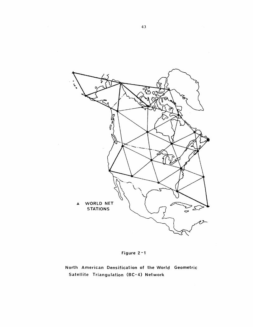
2.2.1 North American Densification of the World Geometric

Satellite Triangulation (BC-4) Network

The results of the completed World Satellite Triangulation

(BC-4) Network were published in late 1974 [Schmid, 1974]. The mean

positional error of the forty-five stations is 4.5 m (lcr). The

twenty-three station North American Densification (Figure 2-1) of the

global network was completed early in 1975 [Pope, 1975]. The solution

of the densification network was carried out independent of the world

net solution, although there are six common stations between the two

of them. The reduction of observations and the adjustment of the

latter network were done in the same manner as for the world network

[Pope, 19751.

The datum of the North American Densification Network is a

set of near-geocentric Cartesian axes. The z-axis was made parallel

to the mean rotation axis of the earth for a certain epoch (CIO) by

virtue of the orientation of the interpolated satellite directions.

The orientation of the X-axis (longitude origin) and position of the

origin were determined by assigning near-geocentric coordinates to

one station in the network. A comparison of the World BC-4 Network

reference frame with that of the WN-14 Global Satellite Results

[Mueller, 1974(b)l indicates that they are separated by a 14m

translation vector, and that the two systems are rotated by 0~11 in

longitude with respect to each other. In a similar test, this time

with respect to the Doppler NWL-9D system, the translation vector BC-4

to NWL9-D was found to be 30 m and the difference in X-axis

orientation 0~61 [Schmid, 1974].

11. WORLD NET STATIONS

43

Figure 2-1

North American Densification of the World Geometric

Satellite Triangulation (BC-4) Network

44

Now, the sources of error in the BC-4 network are examined.

The principle of satellite triangulation is to combine spatial

directions to satellites and one or more spatial distance measurements

in a three-dimensional triangulation adjustment. In the network

being discussed here, the directions, expressed in terms of right­

ascension and declination were obtained, via a complex procedure, from

photographs of satellites against a star background. The required

spatial distances were determined from precise terrestrial traverses.

The standard deviation of such a spatial direction is estimated to be

0.24 arc-seconds [Schmid, 1972; Schmid, 1974], while the two North

American base lines have standard deviations of 3.53 m and 1.59 m

over distances of 3.5 x l06m and 1.4 x 106m respectively [Schmid, 1974].

There are several sources of errors in the observations.

The terrestrially measured base lines are subject to the errors found

in any terrestrial network (2.1). The direction measurements, which

make up the greatest percentage of observations, have error sources

that may be summarized as being dependent on [Schmid, 1965}

(i} the comparator measurements of stars and satellite images;

(ii) the star catalogue data;

(iii) the time determination associated with star and satellite image

exposures;

(iv) atmospheric scintillation;

(v) emulsion distortion occurring during development.

The positional accuracy resulting from rigorous· satellite

triangulation is indepdendent of station location [Schmid, 1965].

45

Internal and external consistency checks have been carried out with

the global BC-4 results. In one internal test, the computed spatial

distances from the adjusted network (one fixed point, one constrained

base line) were compared to precisely determined terrestrial spatial

distances. The total distance difference for the six lines was 9.16 m

6 in a total distance of 17.5 x 10m, or 1.9 ppm (Schmid, 1974].

External checks showed that the network is scaled 2 ppm smaller than

the Doppler NWL-90 solution [Schmid, 1974], and 2.3 ppm smaller than

the WN-14 solution [Mueller, 1974(b)].

Although there are possibilities of unknown systematic errors

in the global BC-4 network, Schmid [1974] stated "error theoretical

investigations indicate that the result, derived in princirle by inter-

polation into the astronomical right ascension-declination system, is

essentially free of systematic errors". Since the North American

Densification Network was established by the same procedures, it is

logical to assume that the aforementioned statement applies to this

network as well. It was expected that the three-dimensional positions

of the Densification could be determined with an accuracy of 3 m to

4 min all components [Schmid, 1970]. The final results yielded mean

standard deviations of 3.4 m, 4.2 m, and 4.7 min the X, Y and Z

components respectively. Computed spatial distances, azimuths, and

6 vertical angles, on lines .83 x 10 .m and greater in length, have

standard deviations of the order of 5.5 m, 0.8 arc-seconds, and 1.0

arc-seconds respectively [Pope, 1975].

46

2.2.2 North American Doppler Networks

The geodetic Doppler networks in Canada and the United

States are expected to contain a total of 350 points upon completion.

In Canada, Doppler points have been established at intervals of 250 km

to 500 km, and by the end of 1974 had numbered 76 (Figure 2-2). These

networks are to be used in the redefinition of the North American

horizontal terrestrial geodetic networks [McLellan, 1974; Strange et al.,

1975].

The nominal reference frame for the Doppler network is the

Average Terrestrial Coordinate System. Studies have indicated that

the origin is within 1 m of the geocentre and that the primary pole

(Z-axis) is oriented such that it is within 5 m, or 0.15 arc-seconds,

of the CIO [Anderle, 1974(b)]. The errors in position and orientation

are largely due to unknown errors in the coefficients used to

represent the earth's gravity field [Anderle, 1974(b)]. The correct

orientation of the longitude origin (X-axis) has not been resolved.

Comparisons with other satellite network reference frames have

yielded relative longitude rotations of up to 1.1 arc seconds (34 m

on the equator) [Mueller, 1974(b)].

The observations being used in the establishment of these

networks are Doppler shift measurements of signals emitted by

satellites of the United States Navy Navigation system. Using

geodetic receivers and a precise ephemeris, recent studies have shown

that three-dimensional coordinates of points can be determined with an

accuracy (lo) of 1 m or less in all three components [Kouba, 1975;

47

• r:: n 0

.... ru ....

(fJ

... C1l

I I

• !

I

I

I

I I N

I

N

C1l ... ::l Cl ·-

.::t:. ... 0 3:: -C1l z .... C1l

a. a. 0 0

-0

-(fJ

48

Hothem, 1975]. The Doppler measurements are subject to several

sources of errors. Typically, the random error in the measurement of

a range difference is in the order of 10 em (Anderle, l974(b)]. The

main sources of observation errors are due to instrument noise, timing,

and ionospheric and tropospheric refraction. In the computation of

coordinates, several effects must be accounted for in order to produce

precise positions. These include orbit determination uncertainties,

data rejection criteria, and the direction of satellite motion

[Kouba, 1975; Hothem, 1975]. The methods used for position computation

are such that several of the unknown errors (orbital biases, timing,

unknown tropospheric refraction) are modelled and solved for simultan­

eously with the position determination [e.g. Brown, 1970; Kouba and

Boal, 1975; Wells, 1974].

The internal and external consistency of the Doppler networks

have been investigated. For example, a Doppler network in Atlantic

Canada was found to have an RMS standard deviation of 0.9 m.

This is compared to 1.2 m and 6.7 m for readjusted terrestrial and

preliminary Geometric Satellite Triangulation in the same area [Wells

et al., 1974]. The scale of the Doppler network in the United States

has been tested against some external standards. When Doppler network

distances were compared to four VLBI distances (0.8 x 106m to 5.0 x 106 m

in length), the maximum difference (Doppler minus VLBI) was 5.1 m.

After scaling down the Doppler distances by 1 ppm, the maximum

difference was 2.1 m [Strange et al., 1975].

As with Satellite Triangulation, the accuracy of a Doppler

network point is not dependent on terrestrial position. Although

49

many solutions yield only point positions with no correlation between

network points, a multistation solution, with.a full covariance

matrix, is possible [Kouba and Boal, 1975]. This type of solution

yields a homogeneous Doppler network in which coordinate standard

deviations are in the order of l m or less.

3. GENERAL CONCEPTS REGARDING THE COMBINATION OF GEODETIC NETWORKS

The problem of the redefinition of the North American_geodetic

networks and the existence of several satellite networks on the cont­

inent requires that some guidance be available to indicate how to use

all available data to solve the aforementioned problems. In view of

this, a general flow chart for the study of the problem of network

combinations has been devised (Figure 3-l) [Krakiwsky and Thomson,

1974]. Investigations involving each of the elements and comple-

tion of the flow is felt to constitute a logical approach to this

study.

The reasons for the combination of terrestrial and satellite

networks are given in 3.1 in the context of how the satellite network

data can be used to supplement classical terrestrial data in the

solution of problems related to the latter networks. A set of parame­

ters by which to classify the mathematical models, in the general

Sense, is given in 3.2. The classifications presented are used as

the basis for the separation of the various combination models given

in this report.

50

HORIZONTAL

NETWORKS 2-D

DOPPLER 3-0

51

OTHOMETRIC

HEIGHTS 1- D

TERRESTRIAL NETWORKS

3-D

COMBINATION OF TERRESTRIAL AND SATELLITE

NETWORKS

Figure 3-1

OPTICAL 3-0

Combination of Geodetic Networks

GEOID HEIGHTS

1 - D

52

3.1 Rationale

Satellite networks provide new and independent sources of

data. Whether or not this data will in fact yield a significant con­

tribution to the solution of terrestrial network problems is dependent

on factors such as the accuracy and homogeneity of the satellite net­

work data and the mathematical model employed in the combination

procedure.

Geodetic datums for terrestrial networks are established

independent of their networks (1.1). The terrestrial networks are

intricately tied to their respective datums, but are in fact separate

entities (2.1). The datum of satellite networks are implied via

various phenomena such as the physics of the model used, the observa­

tions used, and the estimation process (2.2). In this case, the

coordinates of network points can be used to recover the position and

orientation of the datum with respect to some other reference frame.

Due to differences in the establishment of satellite and terrestrial

network datums, their origins will generally not be coincident nor

will their reference frame axes be parallel. In order to be able to

use data from one network as observables in the other, one must use

only that data which is invariant of the coordinate system (spatial

angles and spatial distances) or the datum differences must be modellen.

Datum transformation parameters can be solved for in the

combination of satellite and terrestrial networks. In cases where

the satellite network is the result of dynamic analyses of satellite

observations, the data can be used to assist in the positioning and

53

orienting of the terrestrial network datum with respect to the Average

Terrestrial coordinate system. Further, if the satellite network is

one of global extent, it can be used to relate several regional

terrestrial datums.

Satellite networks are inherently three-dimensional. They

are comparatively free of systematic errors and the relative accuracy

of station coordinates are not dependent on station separation (2.2).

Due to the sequential nature of the establishment of terrestrial

geodetic networks, the relative standard errors of coordinates increases

with interstation distance. There are many unresolved errors in

terrestrial networks as a result of misoriented datums, and scale and

orientation problems in the networks. Satellite data can serve to

strengthen terrestrial networks.

Good quality satellite network data can be used in a terres­

trial network in place of further terrestrial observables. For

example, the older horizontal networks in North America had only

limited numbers of observed base lines and astronomic azimuths for

scale and control of orientation of the network. In addition to

adding scale and orientation control, the use of the satellite network

data in a terrestrial network adjustment will constrain the usual

build-up of random and systematic errors. Intuitively, the result

should be a more internally consistent terrestrial network.

Combination models in which terrestrial network systematic

errors in scale and orientation are modelled are available. These

types of mathematical models do not treat individual systematic

errors of terrestrial observables. Their function is to model, in a

mean sense, the overall effects in a few parameters.

54

In summary, the main reasons for combining satellite and

terrestrial geodetic networks can be given as:

(i) independent source of reliable data;

(ii) strengthening of classical terrestrial networks;

(iii) control of or modelling and removal of systematic errors in

terrestrial networks;

(iv) relating various terrestrial and satellite datums.

3.2 Classification of Mathematical Models

The alternative procedures for the combination of satellite

and terrestrial geodetic networks can be divided into two broad groups:

(i) those in which the datum transformation parameters are considered

known;

(ii) those which treat the datum transformation parameters as unknowns

to be solved for in the combination solution.

Within each of the aforementioned groups, there are four classification

parameters used. They are the dimensionality of the models, the type

of observables required, the parameterization involved in any particular

model, and the estimation procedure used to solve the model.

Due to the traditional splitting of terrestrial geodetic netwarks,

combination models are available that reflect the division. This means

that the three-dimensional satellite data has to be split also. There

are three common types of models - one, two, and three-dimensional.

Table 3-1 is structured around the aforementioned divisions.

55

Several types of observables are used when combining satellite and

terrestrial geodetic networks. One may use all of the original obser­

vables from both networks, or quasi-observables frqm one and the

original observationsfrom the other (Bursa; Table 3-l). Still other

procedures require quasi-observables from two or more satellite and

terrestrial networks.

The unknown parameters in any combination modelare important

in its use and the interpretation of results. Some models contain no

additional unknown parameters due to the combination process (Anderle, Meade;

Table 3-l) . Others contain unknown datum transformation parameters

(Bursa, Wells and Vanicek, Tscherning, Mueller, Lambeck; Table 3-l),

and still others contain these plus parameters to model unknown errors

in one network (Hotine, Krakiwsky and Thomson; Table 3-l).

The estimation procedures vary from one mathematical model

to the other. In many cases the estimation technique used could be

replaced by another method to yield the ~results. Some investiga­

tions require only certain results, thus very simple estimation tech­

niques are employed.

Many studies of the combination of terrestrial and satellite

geodetic networks have been co~pleted. Each of these have employed

only one specific mathematical model. In most instances, little

attention has been paid to whether or not certain models should have

been used. As will be shown later in this report, some of the

accepted combination procedures have been improperly used.

Investi- I Datum Dimen- No. of I Estimation gator(s) Transfor- sionality Observables Unknown Procedure I Remarks

mation Parameters Parameters

Bursa I Unknown 3 Quasi-observables 3 rotations Least-Squares Terrestrial network [1967] from terrestrial Parametric direction cosines

networks Adjustment computed from geode-tic coordinates; those from satellite network obtained from optical observations directly.

Anderle Known 2 Quasi-observables 0 Least-Squares Terrestrial network [l974c] from terrestrial Parametric measurements computed

network; weighted Adjustment from precise geodi-I V'l

Doppler coordi- meter traverses. "' nates

Wells and Unknown 3 Quasi-observables 3 translation Least-Squares Network-coordinates Vanicek from both components Parametric used as observables; [1975] satellite and 4 rotations Adjustment data from several

terrestrial l scale datums is used in networks difference a solution.

Classification of Mathematical Models

Table 3-l.

Investi- I Datum Dimen- No. of I Estimation gator(s) Trans for- sionality Observables Unknown Procedure I Remarks

mat ion Parameters Parameters

Tscherning Unknown I 3 IQuasi-observables 3 translation Least-Squares Terrestrial observables [1975] from both sat- components Collocation included free-air

ellite and gravity anomalies, terrestrial deflections of the ver-networks plus tical and height some terrestrial anomalies. observables

Mueller Unknown 3 Quasi-observables 3 rotations Least-Squares Translation compon-et al (coordinates} 1 scale Parametric ents were considered [1970] from both sat- difference Adjustment to be known.

ellite and terrestrial I~ networks

Merry Known 1 Quasi-observables 1 geoidal Least-Squares Geoidal height deter-[1975] from both sat- height Estimation mined from satellite

ellite and ellipsoidal height terrestrial and terrestrial ortho-networks metric height used as

constraints in geoid determination.

Larnbeck I Unknown I 3 'Quasi-observables 3 tra.nslation Least-Squares Model yields [1971] from both sat- components Combined adjusted coordinates

ellite and 3 rotations Adjustment of common network terrestrial 1 scale points. networks difference

Table 3-1 (cont 'd)

Investi- Datum Dim en-gator (s) Transforrna- sionality

tion Parameters

Meade Known 2 [1974]

Hotine Unknown 3 [1969]

Krakiwsky Unknown 3 and Thomson [1974]

- - - ---

No. of · Observables Unknown

Parameters

Quasi-observables 0 from satellite network

Quasi-observables 3 translation from both sat- components ellite and 3 rotations terrestrial 2 orientation networks parameters

l scale diff.

Quasi-observables 3 translation from both sat- components ellite and 6 rotations terrestrial l scale networks difference

-

Table 3-1 (cont'd)

EStimation Procedure

Least-Squares Parametric Adjustment

Least-Squares Combined Adjustment

Least-Squares Combined Adjustment

- --

Remarks

Distances and azimuths computed from Doppler net-work coordinates.

2 rotations and scale difference are used to model overall systematic errors in terrestrial network.

3 rotations and scale difference are used to model overall systematic errors in terrestrial network.

\.l1 o:>

')9

SECTION fi

COMflTN/\T(ON PROC!mURES Wlll-:N !)/\'!'liM

TW\NSFORM/\'riON Pl\Rl\J'.1ETERS 1\RE KNO\'JN

4. THREE-DIMENSIONAL MODELS

The natural approach to utilizing satellite data is in a three­

dimensional model. With respect to present terrestrial geodetic networY.s

in North America, this is not possible. However, with a view towards

th~ future design of terrestrial networks, it is important to investi­

gate how satellite network data can be used in this mode •

. There are several approaches to entering the satellite data

into the solution of a terrestrial network. One can use the original

observations - directions, ranges, range differences - or some quasi­

observable such as direction cosines derived from this data. Some inves-

tigators have opted for this approach ~n their investigations [Bursa,

1967]. However, the easiest approach is to take the results of the

completed satellite network - coordinates and associated variance­

covariance matrix - and use this information, or some quasi-observables

derived from it, in the combination solution with terrestrial network

data.

Since the datum transformation parameters are assumed to be

known in this instance, the satellite network data can be used in

several ways. For example, one can use the data in a simple model to

60

61

parameterize unknown systematic errors in a terrestrial network. The

data can be added to a network adjustment to supplement the terrestrial

observables and to control the build-up of random and systematic errors.

Several estimation procedures may be employed. For reason=;of

expediency, efficiency, and ease of applic<Jtion, the method of least

squares is suggested here. Of course, different situations may require

either a batch or stepwise approach. Within these bounds, one is free

to choose a parametric, combined, collocation, or any other well known

least squares procedure.

Obviously, many satellite-terrestrial network combination

models within the stated limitations are possible (known datum trans-

formation parameters, three-dimensional models). Given here are several

models which are considered to be practically feasible at the present

time.

4.1 A Parameterization of Scale and Orientation Errors in a Terrestrial

Network

The data required for the model are the Cartesian coordinates

of both the satellite (X., Y., Z.,) and terrestrial (x., y., z.) networks. 1 1 1 1 1 l

These coordinates are assumed to be the results of independent network

adjustments so that each set of coordinates has associated variance-

covariance matrices EXYZ and Exyz The satellite coordinates and their

variance-covariance matrix are transformed to the terrestrial network

coordinate system using the known datum transformation parameters (x , 0

z , 0

£ , X

£ , y

£ ) using the relationsl!if.· (l-9). z

62

The combination model is given by (Figure 4-1)

-+ F 0 (4-1)

where t. is the transformed position vectcr (X., Y., Z.)TG of the satellite l l l l ~)- _,.

point, rk (= pk) is the por:-it ion vector of thf~ tr!rrestrial network

'r . , initial point (xk, yk, zk)G, rki is the terrc~strial network r:osition

T vector with respect to the initial point (xki' yki' zki)G, K is an

unknown scale difference to be estimated, and R represents a product of

three rotation matrices containing unknown network crientzticn parametErs

to be estin:atEd. The matr·ix R is given by

(4-2)

where R1 , R2 , R3 are the well known rotation matrices ((1-11), (1-12),

(1-13)), c.nd ljix, ljiy' ljiz are small rotations about the x, y, and z axes

respectively of a local geodetic coordinate system at the initial point

k, whose axeti arc po.r<J.llcl to those of the Gcoclctic system (Figurr~ 4-l).

Assuming differentially small values for ~x' ~y' ~z' and neglecting

higher than first order terms, (4-2) reduces to

1 ~z -~ y

R -~ 1 ljJX (4-3)

z

ljJ -lj! 1 y X

The reasoning for this model is as follows. First, it is

assumed that after transformation, the differences in the coordinates

of common network points are statistically significant. Second, it is

presumed that the incompatability is caused by the presence of unknown

systematic errors in the terrestrial network. Finally,

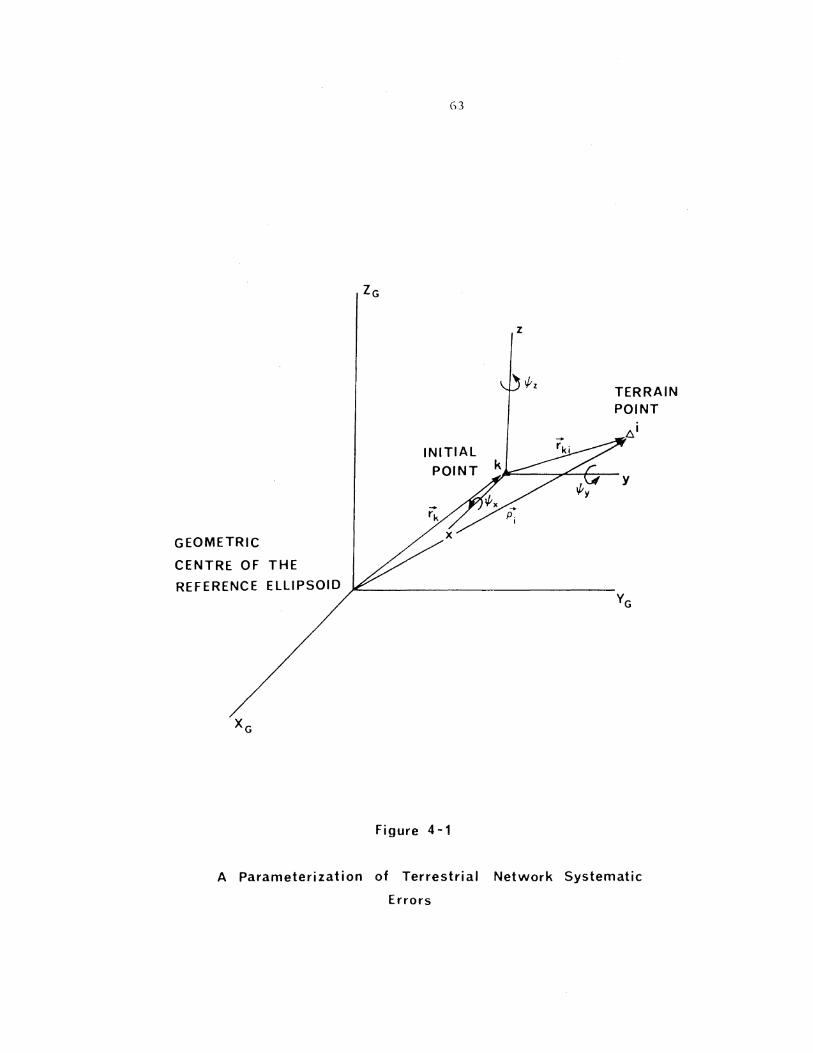
GEOMETRIC

CENTRE OF THE

REFERENCE ELLIPSOID

G3

INITIAL

POINT

Figure 4-1

z

TERRAIN POINT

.6.i

y

A Parameterization of Terrestrial Network Systematic

Errors

()4

difference and three rotations.

The solution to this model can be obtained using a combined

method least squares estimation procedure, expressed functionally as

-F(X, L) = 0, (4-4)

-where X represents the unknown parameters (scale and orientation) and L

the observables (coordinates of common network points) . A linearization

of the non-linear model (4-1) yields the matrix expression

AX + BV + W0 = 0 , (4-5)

in which A and B are design matrices, X is an estimate of the unknown

parameters, V the residuals of the observables, and W0 the misclosure

vector.

F X

Expansion of (4-1) gives

1 X. 1

F y

yk t(l+K) -ljJZ

zk G ljJY

y. (4-6)

Now,

F z -ljJ

1

X

0 assuming that the initial values of the unknown parameters (X ) are

0 zero, the design matrices, A and B, and misclosure vector, W , are given

by

0 -zki yki xki C!F

0 (4-7) A zki -xki yki ax -yki xki 0 zki

65

~ 0 0 I -1 0

_:] aF I

B l 0 I 0 -1 ()L

I () 1 I 0 0

(4-8)

xk + xki - X. l

0 w F (X , L) yk + yki - Y. l

(4-<J)

zk + z - Z. ki l

where L are the observed values of the observables. The solution to

(4-5) is given by [Kouba, 1970; Krakiwsky, 1975]

X

v

Q~ X

-(AT(BE BT)-1 -1 T -1 Wo, L A) (BELB )

ELBTK

(AT (BELBT)-1 A)-1

where the correlate vector, K is given by

(4-10)

(4-ll)

(4-12)

(4-14)

In the above equations, EL is the variance-covariance matrix of the

observables, the coordinates (satellite EXYZ and terrestrial Exyzl of

the common network points. QX and Qt are the weight coefficient matrices

of the estimated parameters and adjusted observables respectively. The

associated variance-covariance matrices are given by

E~ 2 QA = a ,

X 0 X (4-15)

and

E.:. 2 A = a Q-

L 0 L (4-1()

66

2 where a is the a priori vari~nce factor. The least squares estimat0 of 0

the unknown p;~raml't.t'r~ is q i Vt'll l>y

.::. X (4-1"/l

and the adjusted obscrvahlcs (coordinates) by

L = L + V (4-18)

This model, and its proposed solution, is similar to one in

which the datum transformation parameters are considered to be unknown

(7.2). Variations on this theme are possible. If the terrestrial

coordinates are expressed as ellipsoidal (~, A, h), one may wish to

express the orientation unknowns in terms of an azimuth rotation (Q~),

and prime vertical (dp) and meridian (dv) tilts about the Local Geodetic

coordinate system at k. As shown in (7.3), the results are equiv<.~lent

to using ~ , ~ , and ~ as has been presented here. X y Z

4.2 Satellite Coordinates as Weighted Parameters

This is the most straightforward and simple method to combine

geodetic networks. The satellite network data is used directly in a

three-dimensional terrestrial network adjustment, such as that proposed

by Vincenty [1973]. This model requires the adjusted satellite network

coordinates and associated variance-covariance matrix transformed to

the desired coordinate system, and the usual terrestrial observables.

Assuming that a least squares parametric estimation procedure

is used for the network computation, given by

(; 7

F {X) L {4-19)

then the satellite network coordinates are used as initial approximate

coordinates in the formation of the design matrix A and misclosure vector

w. The usual matrix expression for the solution vector is given by

X {4-20)

where L~l is the weight matrix of the observables. However, in this case

there is information regarding the a priori coordinates, which is

characterised by its variance-covariance matrix );XYZ The solution vee-

tor is now given by

-{L-1 +ATL-lA)-1 T -1 X A L W

XYZ L L {4-21)

The final network coordinates are given by

.:; xo ~

X + X (4-22)

and the adjusted terrestrial observables by

~

L L + v (4-23}

where

A

v AX + w (4-24)

The variance-covariance matrix of the adjusted network coordinates is

computed as

E­XYZ

2{~-l AT~-lA)-1 0 o "xyz + "L (4-25}

Through equations {4-21) and {4-25) it is easily seen how the contribu-

tion of the satellite network coordinates are entered into the solution

of the problem. It should be noted that this effect must also be

accounted for in the estimated variance factor (~2 ) by 0

~2

a 0

68

(4-26)

where n is the number of unknown parameters in the network (coordinates

of every point, refraction coefficient, etc.), u represents the number

of observation equations, and nx the number of known satellite determin£!u

coordinates in the network.

This model has several effects on the computation of the network

and its results. First, the knowledge of the coordinates reduces the

number of unknowns in the estimation procedure. If the standard devia-

tions of the satellite determined network coordinates are less than

those of the terrestrial network as computed using only terrestrial

data, the combination of satellite and terrestrial data will constrain

the solution to conform with the weighted satellite coordinate data.

The effect of the constraints is to prevent the build-up of random ~nd

systematic errors in the network The problem is that if the

errors are large, they will propagate into the residuals· of the

terrestrial observables. Existence of problems like this will

show up in a statistical analysis of the results of the network

adjustment.

Such an analysis may lead to an attempt to model suspected

systematic errors in the terrestrial observables. This may include

one or more unknown parameters in scale and orientation. However,

since this type of modeling is not dependent on t~~ use of satellite

network data, it is not covered herein.

When using this model for combining satellite and terrestridl

networks, one must take care with the "fixing" of a terrestrial initiLll

69

point. It is necessary to realize that the variance-covariance matrix

of the satellite network points gives an estimate of the accuracy of

the network coordinates with respect to the datum origin. If one

-+ satellite point (rk) is chosen to be fixed, the variance-covariance

matrix E must be altered to reflect the fact that the satellite xyz

coordinates will have variances, and covariance amongst them, with

respect to the fixed point. This is done using the equation

and the covariance

in which

G

and

E (xyz)ik

law

E (llx

[:

-+ -+ r. - r

l. k

to yield a matrix E ( t\x

T G~ G

tJ.y llz)ik (xyz)ik

0 0 1 0 0

-1 0 0 1 0

0 -1 0 0 1

I (xyz) ik

t\y /Jz) . l.k

l [(xyz)ik I COV ]

I . cov I ~:

(xyz)ki (xyz).k I l.

by

(4-27)

(4-28)

{4-29)

(4-29a)

This procedure propagates the errors of the fixed satellite point into

all others rather than simply, and incorrectly, discarding it.

An alternative to the above is to accept the satellite net-

work datum as the one to be used and let the weighted satellite

network coordinates define it in the network adjustment process. In

this case, no terrestrial points can be held fixed. This is considered

to be a logical solution due to the nature and relationship

of and between satellite networks and their datums.

70

4.3 Satellite Coordinate Differences as Observables

As in the case of usinq satellite nl'l:.work c:oordj natr.s (IS

weighted parameters, the satellite coordinates arc first transformed,

using the known datum transformation parameters, to the desired

coordinate system. Then, observation equations of the form

X .. X. - X. l.J J l.

Y .. Y. - Y. (4-30} l.J J l.

z .. z. - Z. l.J J l.

or equivalently

cpij ~~ . l <Pi

A .. A. A. (4-31} l.J J l.

h .. h. - h. 1.] J l.

are formed. These equations are used to compute elements of the design

matrix (A} and misclosure vector (wPl • The associated variance-covariance

matrix of the observations is given by the covariance law as

E = GE f:J. XYZ

GT , (4-32)

where the elements of G are given by

= [:

0 0 -1 0 :l G 1 0 0 -1

0 1 0 0 -1

(4-33}

The matrix Ef:J. then becomes part of the variance-covariance matrix of

the observables. The network can be solved using a simple least

squares parametric estimation.

71

The major drawback with this approach as compared to that

presented in 4.2 is the extra computational effort required to enter

the same amount of satellite data into a terrestrial network adjustment.

In order to get all information into the solution, it is necessary to write

observation equations of the form (4-30) or (4-31) amongst all satellite

points. Then, the associated variance-covariance matrix must be

generated using (4-32). The comments given in 4.2 regarding the

constraints imposed on the terrestrial network apply here as well.

Another disadvantage of this procedure is that the s · ~llite network

coordinates can not be used to define a datum.

4.4 Computed Spatial Distances, Azimuths, and Vertical Angles as

Observables

This model requires that the spatial distances, azimuths,

and vertical angles computed from the transformed satellite network

coordinates be entered as observables in the three-dimensional

terrestrial network computation procedure. The spatial distances are

given by

s .. ~]

2 ((X.-X.)

J ~

. 2 + (Y. -Y.)

J ~ (4-34)

The azimuth (a .. ) and vertical angle (V .. ) , expressed in the Local ~] ~]

Geodetic coordinate system at i, are given by [Krakiwsky artd Thomson,

1974]

a .. ~]

-1 tan

Y .. (_2:2) X .. ~]

(4-35)

v .. l.]

. -1 s1.n

72

z .. c-.2:.2 > s ..

1.]

(4-36)

In (4-35) and (4-36), the coordinate differences (X .. , Y .. , Z .. ) are 1] l.] 1]

l'XI'rt'~;~;l'd in the J.oc.::tl Geodcl i.e Coordinate sysl.r~m, For qenc~ration

of the associated variance-covari.::tncc matrix, which requires the usc

of coordinate differences in the chosen Geodetic coordinate system,

the equation

X .. -sin 4>i cos A. -sin 4>i sin A. cos 4>. X .. l.J l. l. l. l.J

Y .. -sin A. cos A. 0 Y .. (4-37) l.J l. l. l.J

z .. 'JG

cos 4>. cos A. cos cp. sin A. sin cpi z .. ,... l.J l. l. l. 1 l.J "'

must be used. This leads to the transformation matrix, Gsav' to be

used in the covarinnce law (4-32), given by

. 1s .. ~lS .. iJS .. ilS .. ilS .. ilS .. __Q __Q _2:]_ ___2.1_ __Q --~ .... L ;-~x. ;)y_ :17.. dX. i)y. ;)?,_

1 1 1 J J J

da .. da .. aa .. aa .. aa .. a a .. G :a ~ l.J ....2.2 ....2.2 ---.2:2 ---.2:2 (4-38)

SaV ax. ~ az. ax. av. az. l. 1. 1. J J J

av .. av .. av .. av .. av .. av. _22 _22 _2] ....2.2 ..........2:2 __2i ax. av. az. ax. ClY. az.

1. l. l. J J J

Obviously, this model inputs an equivalent amount of information

compared to the previous two procedures (4.2 and 4.3) if distances,

azimuths, and vertical angles between all satellite network points are

used. Again, the major problem is the extra effort to be expended to

get the same results.

as

73

Anderle [l974(c)] USt.o'd a combination of this model and thilt

presented in (4.:.!) in combin1nq portions of till' llnited Statl~S Dopplc'r

network und gl'Odimctcr traverse:;. TIH· Doppler coordjncJtcs· were used

as weighted parameters, and distances, azimuths and vertical angles

were computed from geodimeter traverse data. The recommendations as

a result of this test were as follows:

"The North American Datum readjustment should be based upon simultaneous adjustment of Doppler satellite and terrestrial data ..... The vertical adjustment should be made prior to or simultaneously with the horizontal adjustment in order that the strength of the Doppler determinations of absolute height can be used to prevent distortion of the vertical datum at the edges or along spurs which would transfer errors into the horizontal adjustment."

It should be noted that a variation of this procedure is

possible in which knowledge of the datum transformation parameters

is not needed. Spatial distances and spatial angles amongst three-

dimensional network points are independent of any coordinate system.

Satellite network spatial distances are computed via (4-34), while

the spatial angle between any two satellite network interstation

+ . + vectors p .. and p. 0 is given by

1) . 1x.

)- ··)o

l p. . • p. n - L l 1 <-COS ( --~-----) (4-39)

1·; .. 1 l;.o~ 1) 1.<.

In the presently used three-dimensional terrestrial network adjustments

[Vincenty, 1973; Fubara, 1972] the spatial angle data can not be

utilized. If changes were made to accommodate the use as observables

of both distances and spatial angles derived from the satellite net-

work, the effects on the terrestrial network would be similar.

5. TWO-DIMENSIONAL MODELS

\'Jhile any two-dimensional approach to the combination of

satellite and terrestrial networks is not as desirable as the three­

dimensional procedures, there are some practical considerations

involved. In North America a three-dimensional approach is not

possible at present due to the distribution of terrestrial data. It

is therefore necessary to eliminate the height component and associated

variances and covariances from the satellite network data to use the

latter in a horizontal terrestrial network adjustment.

The basic drawback of the two-dimensional procedures is the

partial loss of satellite network information. Covariance amongst the

horizontal (~, A) and vertical (h) components of each network point,

and covariance between the horizontal coordinates of one point and

the height components of all other points, is not taken into account.

Three alternative two-dimensional procedures are presented.

They have been used in this and other studies to generate test results

and are considered to be feasible two-dimensional combination

approaches. The assumptions are that proper datum transformations

are to be applied to work in the chosen Geodetic coordinate system,

74

75

and that the terrestrial network computations are to be carried out

on the surface of a reference ellipsoid.

5.1 Satellite Coordinates as Weighted Parameters

The satellite network coordinates, coincident with the

horizontal terrestrial network points, are used as weighted parameters

in a least-squares parametric adjustment of the latter network.

Assuming that the computations will be carried out in the chosen

Geodetic coordinate system, the satellite network coordinates and

associated variance-covariance matrix must be transformed to the

former system using the known transformation parameters.

The procedure to prepare the satellite network data is as

follows. First, compute (<fl., A., h 1.) from (X., Y., Z.) (if required) 1 1 1 1 1

by the iterative procedure for h. and 4>. [Heiskanen and Moritz, 1967] l. l.

p (X~ + Y~)l/2 l. l.

z. 2

N* tan q,i

l. (1 i -1 - e N*+h) p i i

p hi= - N:~

cos 4>. 1 1

Note that in the first iteration, one sets h

tan <fl. l.

The longitude is given directly by

A. l.

-1 tan (Y./X.).

l. l.

(5-1)

(5-2)

(5-3)

0 sv that

(5-4}

(5-5)

76

Alternately, one may use a closed form solution for the above as

suggested by M.K. Paul [1973]. After this, E , h is computed using <j>,l\,

the covariance law by

whcrL' for ~~;H:h point i

sin <j>. cos A. ~ ~

M.+h. ~ ~

sin >... G

~

(N~+h.) cos <l>i ~ ).

cos <l>i cos >... ).

sin

G E XYZ

4>. sin ~

M.+h. ~ ~

cos >... ~

(N~+h.) cos ). ).

cos <j>. sin ~

>... ~

<j>. ).

A. ).

cos 4>. ~

M.+h. .~ ~

0

sin <j>i

(5-6)

(5-7)

The result of 5-6)is a fully populated variance-covariance matrix

E~>..h whose elements, for each set of ~oints i and j, are

0 <j>.>... ~ ~

a cp.>... ~ ).

2 0>...

~

cov .. )l.

a cp.h.

). ~

(5-8)

-1 This matrix, Eq,>..h (5-8), is inverted to yield a weight matrix, E<j>Ah'

pertaining to the satellite network coordinates. To be used in the

two dimensional terrestrial network adjustment, the rows and columns

77

pertaining to the ellipsoidal height are rigorously eliminated during

the inversion process.

The idea of this model is to use satellite coordinates that

have an accuracy that will tend to constrain the usual build-up of

random and systematic errors in a terrestrial network. These errors

will now overflow into the residual and solution vectors. Unfortunately

if the residuals increase too much, the adjustment may not be

accepted as a result of some statistical testing (such as an analysis

of variance} .

The two-dimensional model has been used in some studies of

the combination of North American horizontal terrestrial and Doppler

geodetic networks. In one United States study (Dracup, 1975], five

weighted* Doppler positions were used in a 1566 station network. The

results of several adjustments, with and without the Doppler network

data, were compared to see what the effects were on the network. In

his conclusions, Dracup [1975] stated

" ... geodesists have a powerful and accurate tool, in the form of Doppler positions, for strengthening existing networks and for establishing the fundamental framework in those areas which are now devoid of control, to which conventional geodetic networks may be fitted. Although the inclusion of Doppler positions cannot eliminate observational problems, there are occasions where it might be possible to uncover poor observations or network geometry not previously suspected".

In a similar study [Chamberlain et al., 1976] weighted Doppler

positions helped to determine network scale differences of 2.3 ppm

-1 * No information regarding the computation of E~A was available.

78

when using geodimeter or tellurometer measurements, and an azimuth

orientation discrepancy of "iLS arc-secunds. Further discussion

10. 1.

As with the three-dimensional model of this type, variations

of it can be implemented. For example, the chosen terrestrial

geodetic coordinate system may be that of the satellite network

thus eliminating the need to transform the coordinates and their

variance-covariance matrix. Again, the argument of whether or not

to "fix" one point as a terrestrial network initial point enters

the situation. The steps to be taken, and the implications, are

the same as those given in 4.2.

5.2 Satellite Coordinate Differences as Observables

The steps outlined in 5.1 regarding the application of

transformation parameters to the satellite network coordinates and

their variance-covariance matrix must be carried out. Observation

equations of the form

lj> •• lJ

A .. lJ

A. J

(5-9)

A. 1

are computed. Weights of the quasi-observables are computed via the

covariance law in the same manner as described in 4.3. These weights

are added, in appropriate locations, to the weight matrix of observables,

79

E , to be used in the least-squares parametric adjustment of the L.

terrestrial network.

This procedure adds equivalent information to the terrestrial

network as the method of weighted parameters as long as coordinate

differences amongst all network points are included. As with the

three-dimensional model of this type, the added quasi-observables will

constrain and strengthen the network. This can help to determine

weak points in the terrestrial network, and add some scale and

orientation information.

The major drawback with this approach is the extra compu-

tational effort required to obtain the same results as those of 5.1.

5.3 Computed Distances and Azimuths as Observables

The major problem here is to compute the required ellip-

soidal distances and azimuths and their variance-covariance matrix.

The most rigorous approach is to compute the ellipsoidal coordinates

of the satellite network points (¢., A.) and their variance-covariance L L

matrix E¢A. Then, using rigorous ellipsoidal formulae (e.g. Bamford,

1971; Krakiwsky and Thomson, 1974], compute the geodetic distances

S .. and azimuths a .. amongst all satellite network points. It should L] L]

be noted that the a .. are geodetic, and not astronomic azimuths. This 1]

means that they are not subject to computation via the Laplace

equation (1-7). The quantities are then used in the formulation of

distance and azimuth observation equations for the least-squares

parametric terrestrial network adjustment.

80

The associated variance-covariance matrix of the quasi-

obscrvables, \' '' I Stt

is obt.titll'<l vi.t

l: Sa

T G

Sa (5-11.)

in which }~$>- is obtained simply by eliminating from l:<j>>.h (5-8) those

elements that pertain to the ellipsoidal heights. The elements of G sa

are given adequately by using spherical approximations for S .. and a .. , l.J l.J

namely

in which

s .. 1.)

0. .• l.J

R8

-1 cot S

R = (R, +R.) /2 I

1. J

where Fi and Rj are the Euler radii of curvature, and

0 -1

cos (sin~. sin¢.+ cos¢. cos¢. cos (>..->..)), 1. J 1. J Jl.

tan$. cos$. -sin$. cos (>..->..) J 1 1 J l.

G is computed by sa

where

sin (>..->..) J 1

as .. _2:2 a<J>.

1.

ao. .. _22 a<J>.

1.

as .. _2:1. a>..

l.

ao. .. _2:1. a>..

l.

aa .. _2:1. 3$.

J

as .. _2:2 a>..

J

aa .. _2:2 aA.

J

(5-12)

(5-13)

(5-14)

(5-15)

(5-16)

(5-17)

81

as.. -R

__2:2=--- (cos <fl. sin¢>.- sin <fl. cos <fl. cos (A.-A.)),(5-l8) a <P. sin 8 ~ J ~ J J ~ ~

as.. -R ~) ---­

~-sin 0 i

(cos¢>. cos¢>. sin (A 3. ~ J A. l l ~

( 5-19)

(sin<j>. cos cfJ.- cos¢>. sin cf..cos(A.-A.)) ,(5-2fJ) l. J l. J J l.

as.. -R l.J ---­

~-sin 0 J

a a. . "} ~] . ~

-- = sJ.n a .. acp. ~J ~

(-cos

tan

<P. cos <P. sin ~ J

<jJ.sin¢. cos ~

sin (A.-A.) J l.

<la{j _ . 2 (-s_i_n_(_A~·---A~i_>_s_i_n __ ¢~i--a"f:--- -s~n al2 ( . (' ' ))2

~ s1.n 11.-11.

J l.

(A. A.)) J ~.

(5-21)

<P.cos (A.-A.) ~ ~

) , (5-22)

(5-23)

+cos (A.-A.) (tan cjl. cos <fl.- sin ¢.cos(A.-A.) l. l. ~ l l. ), 5 ___ ..L._.,__ ( -7.3)

a a .. __2:2 <l$.

J

a a .. l] -

Tij-

2 sec <P . . cos. <P .

. 2 l] l. -s~n <1.2 ) (5-24)

sin (A.-A.) J l.

sirf(A. -A.) sin<fl. -. 2 ( J l.

-sl.n al2 2 (sin (A.-A.))

J l.

cos(A.-A.) (tan <fl. cos¢>.- sin ¢>.cos (A.-A.)) J ~ J ~ ~ ~ ) . (5-25)

An alternative approach is to compute the spatial distances

and azimuths, in the geodetic coordinate system, amongst all network

points using (4-34) and (4-35) respectively. These computed quantities are

82

then projected to the reference ellipsoid using rigorous methods [e ·'.!·

Bamford, 1971; Krakiwsky and Thom~;on, 19741, noting that the ;1zimut It:;

need no correction for the (lc•flt•ct.ion of tltc vertic.ll. 'I'll<' tr.111:;-

formation matrix G* requin•tl for <·rror propaqation is <J<~n<~rat.ect vi:J S<l

equations (4-34) and (4-35) to yield

X .. - _2:.1.

s .. lJ

y .. - _2:.2

S .. lJ

z .. - _2:.1.

s .. l)

I I I I G* =

Sa sin .\.X .. -cos

l lJ ¢.cos

l A. y .. cos

l l] A. X .. -sin ¢.sin

l lJ l A. y ..

l lJ cas cp. Y .. I

1 lJ 1

I I I I I I ,-1

2 X .. + l)

X .. 2.2 s ..

l]

2 Y .. l)

sin ,\.X .. +sin l l]

2 2 X .. + y .. l] l]

<fl. COS l

,\ . y .. _l lJ

cos

2 X .. lJ

Y .. _2:.1. s .. l]

2 + y ..

lJ

.\ . X . . +sin <r . ~"in l l] l

2 2 X .. + Y .. lJ lJ

t-.Y. l lJ

2 2 I X .. +Y .. lJ lJ 1

z .. _21_ s .. l']

cO:i •i•. I. ----:l:- .l J

2 2 X .. +Y.

lJ l J ( 5-26)

in which the coordinate differences (X .. , Y .. , Z .. ) are expressed in lJ l] l]

the chosen Geodetic coordinate system. The variance-covariance matrix

is then given by

* I Sa

G* I G*T Sa XYZ Sa

( 5-27)

This approach is based on the assumption that the projections of S .. l]

and a .. are carried out without introducing any errors, and that the l]

distances and azimuths so deduced will not differ significantly from

the quantities computed using ellipsoidal coordinates in rigorous

ellipsoidal geodetic formulae. In some test computations (10.2) in

which satellite station separations of up to 1000 km exist, maximum

83

differences in the distances and azimuths computed via the two afore-

mentioned procedures were found to be 0.29 m (0.3 ppm) and -0.842 arc-

Sl~conds re~•pe·ctivcly. The maximum diffl·n·ncl' in !;Landanl dev.iatiou~;

of the qua~;i-obscrvabl<~s, cumpuh~d usinq G .md G* wen' found to !Jr, · Srt Srt

-0.01 m for distances and -0.204 arc-seconds for azimuths.

The effects of this model in a terrestrial horizontal

geodetic network are the same as those of 5.1 and 5.2, as long as all

data is utilized. The extra computational effort over either of the

previous two alternatives is obvious.

Meade [1974] used this two-dimensional model in a combination

of portions of the United States terrestrial and Doppler geodetic net-

works. In two separate network adjustments, one controlled by

conventional terrestrial base lines and astronomic azimuths and the

other by azimuths and distances computed from four Doppler positions,

he found mean differences or 10 ppm in scale and 0.45 arc-second:;

in azimuth. Further investigations, using the aforementioned com-

parison of network adjustment results, brought to light an azimuth

discrepancy of 3 arc-seconds in a portion of the terrestrial network

[Dracup, 1975].

G. ONE DIMENSIONAL MODELS

As pointed out . r .111 ) 1 horizontal coordinates ( 'f!, > ) and the: i. r

v.-Jt-i.-ltl<'<'-,·ov.tri;uH:<' m.1trix l'•tl"l he easily r~xt.rar:ll:.,d from thr: thrr.:r~-

dilll<'tl:;intt.tl l'.trt,·:-;i;tn co<>nli.ndtr•:-; anrl d!i:-;uciilt:r:d vari;Htr;r;-r:cJV•"Jri;JT,,:,:

m;ttxix ot a :;.tt.<•ll iL<' nc'Lwork. Similarly, tltr· llciqht component~:; (h)

.-tJHl Llll'it- v.tri.IIH'<•-covarianc<: mi!Lrix can ll<' split from the: origi.n.·tJ.

data. Tile obj<~ctivc here is to examine briefly the possiuilitir::.; of

utilizing this height data in combination with terrestrially detcrmi n•:rl

height information.

Again, the loss of covariance can be detrimental to this typt:'

of approach. Whether or not the discarded covariance between height

.111rl h•>ri.zont.JI. C<>nrd.inu.tc:; i ;; s.iq11 i ficant

'l'ilis <:ould CJ!ily lH~ dr·t:,:nni.nr:rl thrn:F]''

some numerical testing in which tltc: same data is US(:d for lJuth a t i<r("

dimensional combination and then separate two-dimensional and o:10-

dimensional combinations.

fl4

85

6.1 Vertical Networks and Geoidal Heights

The information used in the combination of satellite and

terrestrial height networks comes from the equation

h = H + N (6-l)

The ellipsoidal height (h) is obtained directly from satellite

networks. Using known datum transformation parameters in equation (1-~),

the satellite network coordinates are transformed into the desired

geodetic coordinate system. Then, using the procedures outlined in

5.1, the satellite network coordinates (~, A, h) and associated variance­

covariance matrix are computed. From these, the ellipsoidal heights

and variance-covariance matrix are extracted. In satellite networks

already completed, such as the North American Densification of the World

Geodetic Satellite Triangulation, the mean standard deviation of the

ellipsoidal height is of the order of 7 m [Pope, 1975]. The results

in Doppler networks are much better, yielding standard deviations for

h of 0.6 m to 1.6 m [Kouba, 1976(b)]. In a recent paper, Kouba [1976(a) ].

has described a procedure termed "Doppler Levelling" by which height

differences between stations 50 krn apart can be determined to 0.4 m

(l a). Further, he proposes that with improvements in instrumentation

and error modelling Doppler Levelling will yield height differences

with standard deviations of 0.2 m or less for the previously mentioned

station separation.

The orthometric heights, H, of points in the North American

networks are determined as outlined in 2.1.2. Using the rule of thumb

given in 1.3, the standard deviation of the orthometric height difference

between stations 50 km apart would be of the order of 0.02 m. This is

The results of some recent ustrogravi.mctric geoid computations at the,

University of New Brunswick indicate that the geoidal height difference

can be determined with a startdard deviation of the order of 0.5 m for

stations 50 km apart (Merry, 1975]. This accuracy is of the same order

as those presently attainable for ellipsoidal height differences by

Doppler Levelling.

In <·ombininq tl•rn·:;t-rial and satcll ite vertical nc~tw(JrY.~;

l<'ITt·:;lt·io~lly dt·l•·nnirl<·d orllronu·t.ri•· li<~iql!l.:; .111d :-;;tl:c·ll itc: clc~tr:nnirrc:rl

t•llip:;(lirl.JI IH·i.qlits (tr,rn~;formcd to th<• de>;ir<'d geodetic coordinate~;

system via known transformation I:Jarameters) (G-1) yields geoidal

heights. These geoidal heights, with a ~ 0.5 m, can then be used as N

constraints in geoid computations (Merry, 1975]. The second approach

is to use geoidal heights combined with satellite network ellipsoidal

heights to yield orthometric heights. The resulting orthometric hei.(~r.:.

with standard deviations of the order of 0.5 m, could be used for the

reduction of observablcs in ter.rcstrial horizontal networks. Thr:::y "'rJ•::r;

also be of sufficient quality to be used as part of an orthometric height

network. For example, such heights would have sufficient accuracy to

be used in a 1:50000 mapping program.

The conclusion here is that the combination of t•.:ru::-;trj,,]

and satellite vertical networks arc best utilized in supplying ca~-

straints for geoid computations. The accuracies of satellite dE,tE:rmi;,.,c;

87

ellipsoidal heights and geoid computations have not reached the stage

where the resulting orthornetric heights can be used for more than

"lower" order vertical information.

BS

SECTION III: COMBINATION PROCEDURES

WHEN DATUM TRANSFORMATION

PARAMETERS ARE UNKNOWN

7. STANDARD MODELS

The determination of datum transformation parameters is a

three-dimensional problem. The rigorous combination of terrestrial

and satellite geodetic networks will yield the transformation para-

meters between their respective datums. Satellite networks are

immediately ready to be combined, while classical terrestrial net-

works must first be made three-dimensional (1.4) before they can be

utilized.

Several models have been developed which describe the

functional relationships between pairs of three-dimensional coordi-

nates. In each, the network Cartesian coordinates are used as quasi-

observables and thus receive corrections as a result of the combination

estimation procedure.

Three mathematical models, noted as "standard" due to their

extensive use over a number of years, are given herein.* The models

differ from each other in several ways, including a priori conditions,

the type of coordinates used, and the interpretation of results. These

differences, and others, are examined fully in 7.4.

* The names given to these three models - Bursa, Molodensky, Veis -have already been used by several authors. This practice is followed here and is not meant to indicate who may have been responsible for

the original derivation of the models.

7.1 Bursa

The Bursa model [Bursa, 1962; Wolf, 1963; Badekas, 1969;

Lambcck, 1971] expresses Uw relationship between two coordinate

systems by three translations (x , y , z ) , three rotations (c , c , 0 0 0 X Y

t. ) , and a scale change {K). The two sets of network coordinates for z

clny ll'rr<l i 11 point i arc uscxl as observables i 11 thf~ model 9iven by

{l"iqun,7-l)

, ... I

0 . (7-l)

-)-

In the~ above, r is the translation vector between the origin of 0

coordinate systems l and 2, R is the matrix given by [

R r:

(7-2)

where R1 , R2 , and R3 are the rotation matrices given by equations

-)- -)-

(1-ll), {1-12) and {1-13), and r>- and r. arc the position vectors of 1 1

the terrain point i in coordinate systems l and 2 respectively.

Expanding {7-2) as in 4.1, and substituting in {7-l) yields

F X 1 r -(. X, X, X 0 z y 1 1

f' Yo + (1+K) -r: 1 L y. y, 0 ( 7- '3) y z X 1 l

F z c -c 1 z. z. z 0 l

y X l l 1 2

This model is solved easily using a combined case least squares

estimation procedure (4.1). The elements of the design matrix A

are given by

TERRAIN POINT

GEOMETRIC CENTRE OF THE y2 REFERENCE ELLIPSOID

yl

Figure 7-1

Bursa Model

A. ~

-+-dF,

1.

ax-1x,L

1 0

0 1

0 0

92

o I o I o

0 I (z. +K z.)

I ~ o ~ 1 ~-(y,+K y.)

~ ~

- (z. +K0 z.) (y. +K0 y. )l(x. +e:0 y. -e:0 z. >l ~ ~ ~ ~~~z~y~J

o I o o 0 -(x.+K x.) (y.+e: z.-e: x.) ~ ~ ~ X ~ Z ~

o I o o (x.+K x.) 0 l(z.+e: x.-E y.)

~ ~ ~ y ~ X ~

(7-4)

where the superscript 0 indicates initial approximate values of the

unknown parameters, X. Similarly, the dc'sign matrix B is given hy

(l+K0 ) 0 0 0 (EO +KOEO) -1 0 0 -+ (E +K E )

dF, z z y y ~ 0 0 0 0 0 0 0

0 -1 0 B. dLiiX,L

-(E +K E ) (l+K ) -(E +K E ) ~ z z X X

-(e:;O+KOEO 0 0 0 (l+K0 ) 0 -1 (E +K E ) 0

z y X X

(7-5)

If the point of expansion is taken as

(Xo)T (x 0 0 0 0 0 0 Ko) , yo, z , E , E , E , 0 , 0 0 X y z

(7-6)

then A and B reduce to

1 0 () 0 -z. Y. X. l 1 1

A. 0 l 0 z. 0 -x. y, 1 ~ .L 1

(7-7)

0 0 1 -y. X. 0 z. ~ ~ 1.

[:

0 0 -1 0

_:J B. 1 0 0 -1 (7-8) ~

0 l 0 0

The misclosure vector is given by

'tf = F (X0 , L) , (7-9) ~

93

which in this case is

X. - X. ~ ~

vP. yi - Y. (7-10) ~ ~

z. - z. ~ ~

The results of the estimation procedure are the solution vector, X,

the residual vector, V, and their associated variance-covariance matrir~c,~;,

E~ and E~. The final results are the transformation components, X, X V

given by

X (7-ll)

and the adjusted common network coordinates,

L L + V (7-12)

Their respective variance-covariance matrices are given by (4-.15) and

(4-i6).

The use of the coordinates of common network points as

observables is important in the analysis of this model. This is

valid when the networks are relatively free of systematic errors. If,

however, one of the networks contains systematic errors,

these unknown errors will be confused with the datum transformation

parameters. Furthermore, this approach assumes that the network

coordinates can be used to recover a datum. As explained earlier

(3.1), this is true for satellite networks and their datums. The

conclusion drawn here, as a result of a study of the model and the

generation of several sets of test results, is that the Bursa model

is adequate for the combination of two satellite networks, but not

for a terrestrial and a satellite geodetic network.

94

Variations of the Bursa model can be achieved by solving

for fewer unknown parameters. For example, if it is suspected that

the two coordinate systems involved have a scale difference, and arc

translatect parallel to each other, one need only solve for these!

four· parametl•rs. Other combinations of unknowns are possible~ and 111

many instances tests should be carried out so as not to try and solvc~

for more unknown transformation parameters than are really present.

7.2 Molodensky

This model is given by [Molodensky et al., 1962; Badekas,

1969; Mueller et al., 1970]

·+ ~ .• +

F. I ( r o) 1 + ( r k) ;~ + ( .l +K) R ~~ ( r k i) 2 0 . (7-13)

)-

'rhe newly introduced vector rk is that of the "initial point" of U1c:

second network. The quantity Rljl is a combined rotation matrix

(7-14)

where R1 , R2 and R3 are the rotation matrices given previously (4.1).

-+ The vector rki represents the position vector differences of the

second network (Figure 7-2). In an expanded form, (7-13) becomes

F X xk 1 ljl -lj! xi-xk X. X 0 z y 1

F Yo + yk + (l+K) -ljl 1 ljlx yi-yk Y. 0 . (7-15) y z 1

F z zk ljly -ljl 1 zi-zk 2 z. z 0 1 X 1 1 2

The solution of this model is easily obtained using a

combined case least squares estimation procedure (4.1). The solutior,

x,

INITIAL POINT

z

POINT

GEOMETRIC CENTRE OF THE REFERENCE ELLIPSOID y 2

yl

Figure 7- 2

Molodensky Model

96

v~r yields up to seven parameters (three translations, three

rotations, and a scale difference), and a residual vector whose

elements are corrections to the "observed" coordinates and coordinate

differences. The design matrix A is given by elements

A. ~

where

;JF. ~ -10 ax x ,L

l 0

0 l

0 0

Similarly, B is given by

B. .1 .... t !lF

i = 00 (}L. I xo I ~ , "

o 1 o I

0 I zki

l 1-y . I k~

0 z , 0

0 0

l 0

0 l

0 and the misclosure vector r,q by

0

0

-: _: :] 0 0 -1

0 w. ~

yk + y . - Y. k~ ~

I xk. I ~

I Yki

I I zki

0.

(7-16)

(7-17)

(7-lP.)

(7-19)

The model requires the position vector of the initial point of the

second network and coordinate data for at least three other common

points.

The rotations and scale difference in this model refer to

the geodetic network. This fact is obvious upon examination of the

design matrix A, whose elements are the coordinate difference vectors,

.... rki" The main problem is that coordinate systems one and two are

97

assumed to be parallel. This means that all rotation errors ,,n. _._

attributed to the network difference vectors rki' As with the Bursa

model, this type of approach leads to the conf11sion of two :wts uf

rotations - those between the coordinate systems and those associated

with the second network. Also, it should be emphasized that the scale

difference in this model is a network scale difference (note the last

column of the design matrix A. (7-16) which refers to the network ~

+ position vectors rki) .

This model is not used to combine two satellite networks

since in most cases these networks have no network initial points.

Furthermore, in the transformation between two satellite networks, no

a priori assumption regarding parallelity of axes is made.

If the Molodensky model is used to combine a terrestrial and

a satellite geodetic network, the a priori assumption of parallelity of

datum axes may be erroneous. Further, the rotations referring to the

misaligned coordinate axes and those referring to the misoriented

terrestrial network will be confused.

7. 3 Veis

The Veis model (Veis, 1960; Badekas, 1969) is mathematically

equivalent to the Molodensky model. The rotations, denoted dA,

d~, dv, are referred to the Local Geodetic coordinate system

at the initial point k (Figure 7-2). A rotation about the ZLG

axis, dA, corresponds to a rotation in azimuth, about the Y LG

axis, d~, a tilt in the meridian plane, and about the X axis, LG

98

TERRAIN POINT

Figure 7 - 3

Veis Model

TERRESTRIAL INITIAL

POINT

99

dv, a tilt in the prime vertical plane.

where

-+ F.

l.

The model is expressed as

(7-20)

~ R3 (180-Ak) R2 (90-~k) P2R1 (dv) R2 (d~) R3 (dA) P 2 R2 (~k-90)R3 (Ak-180).

( 7-2 J )

the initial point, and P2 is a reflection matrix given by

(7-22)

The first set of rotations, R2 (~k-90) R3 (Ak-180) and the reflection

. -+ P2 , are required to transform the d1fference vector rki to the

Local Geodetic system at k from the coordinate system (2) in which

they are formulated. The rotations R1 (dv) R2 (d~) R3 (dA), in which

dA, d~, dv are the unknown rotation parameters to be determined,

yield a matrix

(7-22)

The final set of orthogonal transformation matrices in (7-21) are

. -+ required to rotate the transformed d1fference vectors rki back to

the second coordinate system. The final expanded result of (7-21)

is given by

100

l I I

~ sin q,kdA + cos cpkdv I I

-cos cpk sin A dA - cos '\dll + sin tj>ksin A kc'lv I k

- sin •I• d/\ - CO~l •l•kdv I k

I 1 I

cos q,k cos .>.. dA - sin \dp - sin ¢kcos Akdv I k I

I · sin.Akcos ¢ dA + cos .Akd\.1 - sin •ksin >kdv J I k

1 - cos q,kcos .AkdA + sin .Akd\.1 + sin ¢kcos :l.kdv • (7-24)

l The solution of the Veis model is the same as for the

Molodensky model (combined case least-squares estimation). The design

matrix B. and misclosure vector WP are equivalent to (7-18) and (7-19), l l

respect .i Vl' 1 y.

-~

;)F

A. lxo ,L ~ -

()X

The dl'siyn matt. i.x !\. ha~; Lhe form 1

l 0 0 -sin <jlkyki + sin AkCOS

0 1 0 sin <jlkxki - cos ¢kcos

!j>kzki

\zki

0 0 l I -cos q,ksin \Xki + cos ¢kcos .Akyki I

-cos

where

cos .Ak zki -cos q,kyki - sin

sin .Ak zki cos <jl X . + k k~ sin

).k xki - sin ).k yki sin 4>ksin }..k~i- sin

oT X = [x 1 y , z I dA1 du, dv, ~1 = o .

0 0 0

<jlksin AkZ . k~

q,kcos .Akzki

ljlkcos :l.kyki

I xk. I ~

I Yki

l zki

(7-25)

(7-26)

The interpretation of the results are the same as for the

Molodensky model. The Molodensky rotations can be derived from the

101

Veis model. The functional relationships are

wx = -cos q,k cos A.kdA + sin A.kdll + sin ¢'kcos A.kd\1 {7-27)

lj!y -cos q,k sin A.kdA - cos A.kdll + sin q.ksin A.kd\1 , (7-28)

4' = -sin ¢'kdA - cos <jlkdv z (7-29)

'l'IH' iiiV<!r.•a.• nf Lhe above yi<•lc!~; til<• Vei:; rot.<~tion~; in terms of thwa: nf

Molodcnsky, namely

dA -cos A.kcos ljlklj!x - sin >.kcos ljlklj!y - sin rj>klj!z , (7-30)

dll sin >. lj! -k X

cos >.kwy , (7-31)

dv -cos A.ksin ¢'kwx + sin >.ksin ¢'klj!y - cos ¢'kwz (7-32)

The problems encountered when using the Veis model for the

combination of terrestrial and satellite networks are the same as those

of the Molodensky model. This model should not be used for the combina-

tion of satellite networks.

7.4 Comparison of Bursa, Molodensky and Veis Models

Based on the comparisons of the models, and the knowledge of the

· d t ll"t t ks conclusions can be drawn on properties of terrestr~al an sa e ~ e ne wor ,

their respective advantages in the combination of terrestrial and

satellite geodetic networks.

All three models contain a maximum of seven unknown trans-

formation parameters. A solution for each of the models is easily

102

obtained via a combined case least squares estimation procedure. The

Molodensky and Veis models are based on the same a priori assumption

of parallelity of coordinate system axes, and contain explicit provisions fur

a network initial point for the second network. These latter two

+ + models use the same observables- rk. and p .• As was shown in 7.3, the

~ ~

Molodensky and Veis rotations are easily related to one another.

There are several significant differences in the three

models, particularly between the Bursa model,and the Molodensky and

Veis models. The Bursa rotations and scale difference refer directly

to the coordinate systems as is indicated by the elements of the A

matrix (7-4). This interpretation is based on the fact that the two

networks involved can be used to recover the origin and orientation

of their respective datum axes. As argued previously (3.1), this is

only possible in the case of satellite networks. On the other hand,

the Molodensky and Veis models use only one network in this fashion

(the first). The second network observables are network coordinate

differences, and the rotations and scale difference apply to these

quantities. The Bursa model has no provision for an initial point of

the second network at which there are no second network coordinates.

In contrast to the Molodensky and Veis models, all network points in

the Bursa model are treated equivalently. Between the Molodensky and

Veis models, the only difference is the orientation of the coordinate

system at the initial point k. This fact has no bearing on the

solution or interpretation of results.

Comparing the Bursa and 11olodensky models mathematically, one

obtains the difference

103

-+ -+ -+ r r + (QM - QB) 6rik 0 0

o, (7-33) M B

in which

QM R!JI - I, (7-34)

QB = R v

- I, (7-35)

.'l.nd t.h<' subscr.i pts B and M n!fer to thP. 13ursn. and 11olodensky models.

-~

If on" assumes th" two solut.ions will t~ the silmc (i.e. r

K8 ), then one ohtains

0 M

(7-36)

This expression (7-36) is satisfied if and only if Q = 0 B

0. This is further proof of the differences between the Bursa

and Molodensky (or Veis) models.

The main problem with all three models is the assumption of

only one set of rotation parameters. As has been discussed previously,

it is unlikely that two coordinate systems, either satellite and

terrestrial datums, or two Sdtellite or terrestrial datums, would be

parallel. T~us, in any combination procedure, some or all of the Bursa

rotations would be present. When a terrestrial network is involved,

it is known that it would contain errors which may be modelled by

either the Molodensky or Veis rotations and a scale difference.

It should be noted that when combining a terrestrial and a

satellite network using the Bursa and !1olodenskv models, identical

numerical values for the rotations are obtained (see 11.0 and 11.2).

Howe"er, the translation components will differ. The reason for this is

that the scale difference parameter, K, is applied only to the coordinate

differences in the Holodensky model (7-13), while in the Bursa model

(7-1), it is applied to all position vectors, including that of the

terrestrial initial point.

l03a

The conclusions to be drawn are first that two satellite

net,,orks, rcl.1.tive.l v free of ~yste!Tiiltic errors with respect to eG~ch oth,~r,

can be combined using a Hur.s.1 model. This has been done by several

invcstiqn.tors [Anderle, l974(h); Mueller, l974(b)]. The BuY.sa model

i.s not adequn.te for the combination of a satellite and a terrestrial

network, mainly because the one set of rotations does not adequately

model the true situation. The Molodensky and Veis models can not be

used to combine two satellite networks due to the a priori assumption

of parallelity of datum axes and the necessity of having a network

initial point for one of the networks. The latter models may be used

to combine terrestrial and satellite networks since an initial point

would be available for the terrestrial network, and the rotations and

scale difference can model th.-~ errors in this L1.tter network. J!owcv,:r,

the assumption of axes parallelity again makes the models unacceptable.

Basically, all three models - Bursa, Molodensky and Veis -

are inadequate for the combination of terrestrial and satellite networks

for one fundamental reason: ~hey do not contain sufficient transformatior,

unknowns to adequately describe the relationship between the two net•,.orks

and their datums. This inadequacy led to the study and development of

the more complex models of 8.1, -s.2 and 8.3.

8. RECENT MODELS

In 1.3 the problems related to the positioning and orienting

of a terrestrial datum were en~merated and in 2.1 the existence of

systematic errors in the terrestrial networks themselves were pointed

out. When terrestrial and satellite networks are combined and the

datum transformation parameters are known (SECTION II) , the datum

orientation and position problems are not involved, and systematic

errors are assumed to have been removed in some acceptable manner.

However, when datum position and orientation parameters are unknown,

the combination of networks becomes complex. Further, if one attempts

to model the systematic errors in the terrestrial network or to

investigate the parallelism of Geodetic and satellite coordinate sys­

tems with respect to the Average Terrestrial system, other compli­

cations arise.

The Bursa, Molodensky and Veis models (7) are not adequate

for the treatment of the above mentioned problems. The predominant

inadequacy of the aforementioned models is the existence of only one

set of rotations in each. The Hotine (8.1), Krakiwsky-Thomson (8.2),

and Vanicek-Wells (8.3) models do not have this inadequacy as the

models contain two sets of rotations. The first two models are

104

105

formulated such that in the network combination process the systematic

errors in the terrestrial network are modelled by up to three orientation

parameters and a scale di fferen<.:P. Tlw third model (Vanicek-Wells) is

concerned partly with the lack of parallelism of Geodetic and satellite

system axes with those of the Average Terrestrial system.

The data used in each of these models are the adjusted

coordinates of three-dimensional terrestrial and satellite networks.

It may be argued that the Geodetic coordinate system axes can be made

"nearly" parallel to those of the Average Terrestrial system using

classical methods, and that the systematic errors in a terrestrial

network can be effectively modelled and removed during the estimation

process. However, due to the many problems involved, it is unlikely

that the above will be tlw case and it is the common belief amongst

several geodesists that residual model errors will remain in the

datum transformation parameters and the orientation and scale of the

terrestrial network. The models presented herein are proposed as

possible solutions to the removal of the above mentionedresidual errors.

8.1 Hotine

In his monograph Mathematical Geodesy, Hotine [1969] argues

that there should be two sets of rotations in a model intended for

the combination of geodetic networks. His argument for this is

stated as:

"In a.ddition to the initial choice of a discordant system of geodetic coordinates, the network itself may have systematic errors of scale and orientation for which an

106

allowance should be madt~ before Wl~ .l.djust the network to adjacent work or into a fixed system of a worldwide triangulation."

He goes on to state that if there is only one set of rotations in the

combination model, namely those pertaining to the discordant geodetic

coordinate system,

" .•. the effect of a systematic orientation error in the network could be concealed by evaluating false values of the rotation parameters w1 , w2 , w3 ."*

Thus, he makes a separation of rotation parameters (w1 , w2 , w3 ) for the

discordant geodetic coordinate system from the orientation parameters for

the systematic errors in the terrestrial network. The two parameters are

da, a change in azimuth, and dS, a change in zenith distance. The azimuth

parameter, da is a rotation about the z-axis of the local geodetic

coordinate system at the terrestrial initial point k. The zenith distance

parameter, dS, is a constant applied to all lines radiating from the

terrestrial initial point, k. In addition, network scale error is accounted

for by a scale difference parameter, K. Counting the datum translation

parameters, this gives a total of nine unknown parameters in a combin-

ation model expressed as (Figure B-1)

0

+ (rk.) the position

~ , vector of i with respect to the initial point k, is defined in terms

of the vector length l;kil, and the azimuth (aki) and zenith distance

(Ski) in the local geodetic coordinate system at k. The matrix ~

contains the unknown parameters K, da, dS, and is derived below.

The Hotine model as given by (8-1) is expanded as follows:

+ First, rki is expressed by

*Hotine's rotations w1 , w2 , w3·-are equivalent to the values e: 1 , e: 2 , and e: 3 used in this work.

(8-L)

107

Figure 8 -1

Hotine Model

TERRAIN POINT

.o.i

TERRESTRIAL INITIAL POINT

lOH

xki 'l;kil sin ski cos (lki

-+ ,;kil rki yki sin ski sin (lki (8-2)

zki ,-:kil cos ski

-+ 1-+ I -+ After evaluating the partial derivatives arki/a rki , arki/aaki'

:l;k/;11\i, the change in coordinates due to the changes in j;ki j, rxki'

and 1\i can be expressed by

I -+ . ~~-~ I dxki sin 8ki cos akij\rkilsl.n ski sin uki 1 rki cos ski cos aki drki

dyki sin 13ki sin I 1-+

akil rkilsin ski cos aki 11;ki I cos skisin a.ki da.ki

I I _,;kil dzki cos ski I 0 I sin 13ki dSk.

(8-3)

Using the expressions

(8-4)

where the prime (') indicates th<~ changed values of coordinates due

to drki' da.ki' and dSki' and setting

K = I • (8-5)

the matrix ~ is

(l+K) -da. cos a .dS kl.

~ da (l+K) sin a.kidB (8-6)

dS 0 (l+K)

cosa.ki I

109

The expanded model (8-1) is now written as

F X 1 e: -e: xk (l+K) J-da leo sa . dl3 xki X. ·.x 0 z y k~ ~

1 I I

F yo + -e: e: yk + da I (l+K~sinakidl3 yki - Y. y z X ~

F 1 dl3 I I

(l+K) z 1

e: -e: zk cosak .1 0 I zki z. z 0 y X I 2 ~ l

~.

(8-7)

Hotine [1969] also mentions the possibility of including two more

parameters in his model - da and de which are changes in the size and

~hape of the reference geodetic ellipsoid. These have not been

included herein for two reasons. The inclusion of da and de may be

~sed if one were working with the problem of determining the "Figure

of the Earth"(defining the Geodetic coordinate system which best fits

the Astronomic system which is beyond the scope of this work). Further,

the inclusion of da would tend to eliminate the systematic error in

Scale of the terrestrial network since the ellipsoid would be

rescaled to absorb scale errors. As stated by Hotine [1969]

"this procedure would vitiate the height dimension and would result in some inaccuracy even in a two-dimensional adjustment which ignores geodetic heights ..•. ".

Since there are only two networks involved in this combina-

tion procedure the estimation procedure for its solution is not

easily formulated. Hotine did not propose any estimation

procedure for the solution of his combination model. Regarding

the model and its solution, he stated [Hotine, 1969]:

"This procedure assumes that the parameters are independent and that second-order effects can be either neglected or removed by some process of iteration, although in some cases, the parameters, especially the rotations, will be strongly correlated".

0.

110

The estimation procedure proposed for the Krakiwsky-Thomson

model can be used for the solution of the Hot.inc model. The design

matrices and misclosure vector:; are the same as those given in 8. 2

except for A22 _ which pertains to the unknown orientation and scale l.

parameters in the second (terrestrial) network. For the Hotine model,

A22 . is given by l.

A 22.

l.

where

-ykil cos aki 2 ki I

ClF xkil sin --

aki 2 ki - 0 ax21 x2, L2 I

0 1-xki/cosaki

T (da, d8, K) 0 .

xki

yki (8-8)

2 ki

(8-9)

The solution is obtained using the matrix equations given in 8.2.

The Hotine model can be used to combine a terrestrial and a

satellite geodetic network. The solution yields the datum transforma-A A - -

tion parameters x1 , adjusted network coordinates L1 and L2 , three

parameters (X 2 ) which represent the systematic errors in the terrestrial

(second) network, and their associated variance-covariance matrices. The

one drawback of this model is the parameterization of the network

orientation errors. The parameters da and dB can not be split to

give either the Molodensky (~ 1 , ~ 2 , ~ 3 ) or Veis (dA, d~, dv) types of

representation. The latter are particularly desirable if one is going

to compute the changes in the deflection components of the vertical

at the initial point that have occurred due to the combination process.

lll

8.2 Krakiwsky-Thomson

Like the Hotine model, this one contains two sets of rota-

tions - a first set (c , r: , c ) for the" misorientation of the second X Y Z

coordinate system with respect to the first and a·second set ('I' , 'I' , X y

tjJ ) or (dA, d!l, dv) for the misoriented network. When first published z

[Krakiwsky and Thomson, 1974], it was given as

-+ F.

1 (8-10)

The scale difference in the above is interpreted as a system scale

difference. Thus, (l+K), along with the system rotations in R (7-2), £

-+ yields a totally redefined initial point. (rk). Also, the systematic

scale error in the terrestrial network, represented by the vectors

-+ (rki), will be absorbed in the system scale difference. To have the

scale difference parameter apply to the second network and obtain a

parameterization of network orientation errors in terms of azimuth

and tilts in the prime vertical and meridian planes, the Krakiwsky-

Thomson model is written as [Thomson and Krakiwsky, 1975] (Figure

8-2)

+ F.

1 0.

Expanding (8-ll) with quantities previously defined yields

(8-ll)

112

TERRAIN POINT

Figure 8- 2

Kra kiwsky- Thomson Model

d,u TERRESTRIAL INITIAL POINT

113

F X l £ -£ xk X 0 z y

F yo + -r: 1 r: yk + y z X

I·' z -, z ., I) y X k

/

1

+ { l +K)

l

This model contains ten unknown parameters, of which six

are rotations. In order to compute a solution, there must be at least

four network points for which Cartesian coordinates are available in

the two coordinate systems.

Since there are two sets of unknown rotations and only two

networks {one satellite, one terrestrial) are being combined, a special

least-squares estimation procedure is required to obtain a solution.

The estimation model, in functional form, is

where

114

Fl (Xl, Ll) 0 , (B-13)

F2(X1, x2' L )= 2

0, (11-14)

-xl are the coordinate system transformation parameters (x ,

0 Yo'

z o' £. x' £. y' £. ) ; z

x2 are the rotation and scale differences parameters pertaining

to the second network (K, dA, d), dv);

L1 are the observables (coordinate differences (xik' Yik' zikl 2

and coordinates (Xi, Yi, Zi)l of the "inner zone" )(Figure

L2 are the observables (coordinate differences (xik' yik' zik> 2

and coordinates (X., Y., Z.) 1 of the outer zone)(Figure 8-3). ~ 1. 1.

The reason for the splitting of the coordinates of

common points into inner and outer zones is to make the solution

IDssible for the two sets of rotation parameters in the Krakiwsky-

Thomson model. The inner zone contains sufficient observables (L1 )

to solve for the unknown parameters (X1 ). The common network points

of the inner zone should be sufficiently close to the terrestrial

initial point so that the observables (coordinates) of the second

(terrestrial) network will not contain significant systematic errors.

The outer zone then contains the remaining common network stations.

The observables L1 and L2 are correlated. Thus,

the variance-covariance matrix of the observables is given

by

(8-15)

115

(OUTER ZONE)

L2

(INNER ZONE) Ll.i L1

Ll.k

Figure 8- 3

Estimation Procedure for the Krakiwsky- Thomson Model

116

Linear Taylor series expansions of F1 (8-13) and F2 (8-14) yields the

matrix equations

A X + B V + \"1° 11 1 11 1 1

0 , (8-16)

0 , (8-17)

where

The least squares normal equations relating the unknown quantities (X1 ,

0 x2 , v1 , v2 ) to the known quantities (All' B11 , w1 , A21 , A22 , B22 , W2 ,

>:*) are norlTk>lly obtained from the variation function [Krakiwsky, 197r,J L

However, due to the form of the variance-covariance matrix E~ and the

need to invert it for the development of the normal equation system, an

alternate approach has been chosen.

The development given here of the matrix equations required

for the solution of the proposed least-squares estimation model is

similar to that used to derive the stepwise collocation equations

[Moritz, 1973; Krakiwsky, 1975]. A new, and simplified, model

117

F(X*, L*) 0 (8-20)

-in which X* conL.lins x1 ~llld X.,_, and r.* <"OIIl<lin:; 1. 1 .111d 1.;~ a:; will llc'

shown shortly, is ust•d to devel.np Ll••· W1•l.l known c:t>mhi.m~d-,:,_l:;v l.t:a:;l-

squ.:tres mc1trix l'qu.1tions (sec 1:quaUons (ll-1.0) Lo (4-14) inclusive: in

Chapter 4)

X*

V*

K

Q~ L

1:* B*T K* (8-22) L

- (B*Z::* B*T) -l (A*X* + W*) (8-23) L

(A*T(B*Z::* B*T)-l A*)-l (8-24) L

(1:*-Z::*B*T((B*E*BT)-l-(B*E*B*T)-lA*Q.A*T(B*E*B*T))B*Z::*). (8-25) LL L L X L L

:;Lq>wi:a: pruc<·dure n·quin·d for Uw solution whi lr~ m<~intaininq th<:

ct>V<Iridllt"<' bf'tWI'I'Il LIH: i.nr11·r and oul.,·r ZOII<' observahl<·:-;. 'l'h<' unknown:;

and residuals are given by

X* and (8-26)

The weight coefficient matrices are given by

(8-27)

and

Q­L

118

and the final variance-covariance matrices by

l:~ = X*

a 2

0 QA

xl

)'A - 2 Q~ a ·r:*- 0

The misclosurc and correlate vectors are

W* and K*

The hyper-design matrix A* has the form

A*

(8-28)

(8-29)

(8-30)

(8-31)

(8-32)

0 0 When the' ini tiul approximate values, x1 ilnd x2 are set to zero, then

l 0 0 0 -(zk+zki) (yk +yki)

All. 0 l 0 ( z +z . ) k k1

0 -(x +x .) k k~

(8-33) ~

0 0 l -(yk+yki) (xk +xki) 0

for the r 1 observations and u 1 unknowns of the inner zone, the elements

of A21 are computed just as those of A11 for the r 2 observations and u 1

unknowns of the outer zone, and

-cos <Pk yki - sin

cos <Pk xki + sin

sin <Pk sin \ X . kl.

- sin

1'k sin ·\

<Pk cos A k

<Pk cos \

119

zki

zki

yki

xki

yki

zki

S in ' z 1\k ki

(8-34)

for the r 2 observations and u 2 unknowns of the outer zone. The hyper-

design matrix B* is given by

[" 1 I 0 j B* _! __ ~---o I 822

(8-35}

where

{: 0 0 1 0 0 -1 0

-~ Bll. 1 0 0 1 0 0 -1 l.

0 1 0 0 1 0 0

(8-36}

-+ The three sections of s 11 pertain to the initial point (rk}, the

-+ -+ coordinate differences (rki), and the coordinates (pi}. If there are

. -+ coord1nates (pk) at the initial point, then

(8-37)

-+ since rkk 0. The full design matrix, which has dimensions (r1x2r1 }

is given by

(

120

3!3 I - I 3 3

0 0 0 0

31 3 I

0 3!3 -3I3 0 0 (8-38) I Bll 3!3 I 0 0 0 3!3 -3I3 I

I I I I

8 22 is given by

8 22. [3 r 3 lJIJ] (8-39) 1

and the full matrix is

31 3 -3I3 0 0 0 0

0 0 3!3 -3!3 0 0 (8-40)

8 22 0 0 0 0 31 3 -3!3

The misclosure vector, for inner zone points, is

xk + xki - X. 1

0·

wl. yk + yki - Y. 1 1

(8-41)

zk + zki - Z. 1

0 and the elements of w2 are evaluated for the outer zone points using

the same expression.

The solution is now generated using the expanded matrices in

equations (8-21) through (8-25) inclusively. For example, (8-21) is

now

!.:>I

~ I ~T 11 I 0 --,--21 I A22

This expression for the unknown parameters is equivalent to a set of

sequential expressions in which x1 and x2 are solved for in explicitly

separdte matrix expressions.

The Krakiwsky-Thomson model as developed here, or expanded

using Molodcnsky type rotations to express the misorientation of a

network, can be used to combine a satellite and a terrestrial geodetic

network. If the quantities dA, d~, dv are computed, then ~l' ~ 2 , ~ 3

can be computed using (7-25) to (7-25), or vice-versa via (7-28) to

(7-30).

Test results of the combination of a terrestrial and a

satl!llitc network have been gctwrated (12) using the Krakiwsky-

Thomson model as developed herein.

122

8.3 Vanicek-Wells

The stated objective of this model is to enable one "to examine

numerically the parallelism of geodetic systems (based on terrestrial

observations) and satellite systems (based on satellite observations)

and the average terrestrial system" [Wells and Vanicek, 1975]. The

model is given by [Wells and Vanicek, 1975] (Figure 8-4)

(8-4 3)

where rG is the translation vector between the Average Terrestrial and

Geodetic systems, r 5 is the translation vector between the Average

Terrestrial and the satellite systems, K is the scale difference in the

Geodetic system, R~ and Rw~£ are rotation matrices (see below) , and

__ ,.. -> -)-

rk' rki' and pi are as previously defined.

The rotation matrix R , which contains the three rotations wl)J£

of the three satellite system axes with respect to the Average

Terrestrial axes is given by

R W~£

(8-44'

The originators of this model have proven that under certain

conditions only four datum position and orientation parameters exist

(three translations, one azimuth rotation) [Vanicek and lvells, 1974].

This occurs when the orientation and position of the datum is defined

at a terrestrial initial point, at which point equations (l-3) and (1-4)

are accepted by definition. Under this condition, equation (l-6) is

satisfied. This then leaves only the azimuth orientation condition (1-7)

to be satisfied. Thus, the rotation matrix, R~, pertaining to the

Geodetic coord.ilate system contains only the azimuth orientation unknm1r:

~ and is given by [l-1ells and Vanicek, 1975].

Xs

SATELLITE ORIGIN

123

Figure 8-4

Vanicek- Wells Model

ELLIPSOIDAL NORMAL

I 'frtl

k INITIAL POINT

ORIGIN OF REFERENCE ELLIPSOID

1

1

t:,. cos s1.n

124

-t:,. cos ~k sin Ak

t:,. cos ~k cos Ak

1

(8-45)

There are eight unknowns to be solved for using this model

r S(;

The last quantity, the difference vector rsG'

replaces r and r since the ct!ntrc of gravity (origin of the Avcrag<; S G

Terrestrial system) is unknown. As with the previous two models

presented (Hotine and Krakiwsky-Thomson) , this one contains two

unknown sets of rotation parameters. One satellite network and

several geodetic networks, having common points, are combined in one

parametric least-squares solution. Details of the development of the

model and its solution are given in [Wells and Vanicek, 1975].

In some test computations, Wells and Vanicek [1975] have

shown how this model is used to combine one satellite network with up

to five qcocit,tic. Their cone I us ions include the comment that can.!

should be taken in the selection of both data points and datums used

in the application of this model.

8.4 Comparison of the Hotine, Krakiwsky-Thomson, and Vanicek-Wells Models

All three models contain two sets of unknown rotation para-

meters. The observables used in each of them are the Cartesian

coordinates of points common to the satellite and terrestrial networks

involved. The estimation procedure used in each case is the method of

least-squares, although different case~; ;~rc ust'd for the llotinc

and Krakiwsky-Thomson models from the Vanicek-Wells model. Each

model yields the three components of the position vector r 0 (rSG

in Vanicek-Wells) - the translation vector between the origins of the

satellite and Geodetic coordinate systems.

In the Hotine and Krakiwsky-Thomson models, the first set

of rotations (E , E , E ) expresses the alignment of the Geodetic X y Z

system axes with respect to those of the satellite system. The Vanicek-

Wells rotations (w, ~. £) express the alignment of the satellite axes

with r(!sp<'Ct hl those of the 1\veraqc Tern~stria1 sy!;tem. The second

Vanicck-Wclls rotation, A, is that which relates the Geodetic system

with the Average Terrestrial, whereas the Hotine (da, d8) and Krakiwsky-

Thomson (da, d~, dV\ parameters are a parameterization of the systematic

errors in the terrestrial network.

The scale difference parameter, K, is a Geodetic coordinate

system scale factor in the Vanicek-Wells model. In the Hotine model,

it (K) is an expression of the systematic scale error in the terrestrial

network. The Krakiwsky-Thomson model is such that K can be entered to

express either of the above. In the development of the model herein

(8.2), it is treated as an expression of systematic scale distortion

in the terrestrial network.

The Hotine and Krakiwsky-Thomson models have been developed

for the combination of one satellite and one terrestrial network, thus

only two coordinate systems are involved. Both of these can be easily

expanded to accommodate more satellite networks in the combination

procedure [Krakiwsky and Thomson, 1974]. There are·several coordinate

126

systems involved in the vanicek-Wells model - the Average Terrestri:J.l,

ont' satellitt• <tnct several Geodl'tic.

from Lite di ffer:ent objectives of the models. Tit(! llotine and Krakiwr;ky-

Thomson are concerned with the combination of a satellite and a

terrestrial network, the orientation and position of the Geodetic

system with respect to the satellite system, and a parameterization of

systematic errors in the terrestrial network. The objective of the

Vanicek-Wells model is the determination of the orientation of a set

of satellite system axes, and that of several Geodetic systems, with

respect to the Average Terrestrial system. Also included are para­

meters that yield the position and scale of the Geodetic system with

respcc t to tha L of the sate l 1 i t(• ru~twor:k.

8.5 Comparison of Hotine, Krakiwsky-Thomson, Vanicek-Wells Models with

those of Bursa, Molodensky, and Veis

This comparison of models is made on the basis of combining

satellite and terrestrial geodetic networks. This does not preclude

the fact that none of the Bursa, Veis, or Molodensky models are con­

sidered to be adequate for the task (7.4).

All of the models covered in 7 and 8 are three-dimensional.

Datum transformation parameters are treated as unknowns. The obser­

vables utilized in each model are the Cartesian coordinates of points

common to the satellite and terrestrial networks under consideration.

The solutions are obtained using a least squares estimation procedure.

127

In each model, the translation vector, r 0 (rSG in the Vanicek-

Wells model), between the satellite and terrestrial network datums

appears explicitly. The Bursa, Hotine, and Krakiwsky-Thomson models

have an explicit set of unknown rotation parameters between the satellite

and geodetic coordinate systems, while the Vanicek-Wells models solves

for rotatiombetween these two systems and the Average Terrestrial

coordinate system. The Molodensky and Veis models have no provision for

a discordant geodetic coordinate system.

The parameterization of systematic errors in the terrestrial

network is accomplished via three rotations {da, d~, dv or w , W , Wz) X y

and a scale difference in the Molodensky, Veis, and Krakiwsky-

Thomson models. The Bursa and Vanicek-Wells models do not have this

provision.

In the Bursa and Vanicek-Wells models, the terrestrial

initial point is totally redefined, that is, scaled and rotated. The

terrestrial network initial point is rotated but not scaled in the

presented versions of the Hotine and Krakiwsky-Thomson models. As

pointed out in 8.1 and 8.2, the inclusion of {da, de) in the Hotine

model, or having K as a system scale in the Krakiwsky-Thomson model,

would cause a total redefinition of the terrestrial network initial

point.

The major differences in the models are that the first set -

Bursa, Molodensky, Veis - contains only one set of unknown rotation

parameters, while the second set - Hotine, Thomson-Krakiwsky, Vanicek-

Wells - contains two sets of unknown rotation parameters. For this

reason, more complex least squares estimation procedures are required

128

for two of the latter set (Hntine, Krakiwsy-Thomson) while the third

(Vanicek-WQ 11 s) involves sev< · r,-d t.crn·s trial qendeti c datums.

r.~,- lll<•t··· fl··xihl<· tltdll t:ilv 1\lil'!i.l, 11o>lod<'tl!iky, dtlcl V<_·i.!-i m<><l!!l!i, ;Ill•!

will Lllli!i mon.! C.J!;j.\y rcfJecl pl:ysica.l I"l!illity.

'l. ::IJMMJ\HY

Ft.Hlrle<•n mathematical models for the combination of

terrestrial and satellite networks have been examined. The examination

of each model has been carried out under the terms spelled out in 3.2.

Where necessary, a complete development of the models has been presented.

The purpose here is to surrunarize, in three Tables (9-l, 9-2, 9-3), the

charact:erist i.cs and recorrunendt~d uses of each of the models.

'f'lll · Tables arc· ~~1'1 1 t in to two major :;cqmcn t s. The: fir~; t

(T,tJJ!,. 'l-l) ,·over:; :;<·V<'Il <lf IIH' (~.l(jht model~,; studied in which the di.!tum

the models can b(' used. The :;L•cond segment (Tables 9-2 and 9-3)

includes all six models inveo;tigated in which some or all cf the" datum

transformatian parameters arc S()lVf:d for during the combinatic.on pro<_e:.··

For the six models given in Table 9-l, there are four major

features outlined for each model. These are Dimensionality, Unknown

Parameters, Observables, and Estimation Procedure. The use of each

model is the combination of a satellite and a terrestrial network.

The implementation is given by the name of each model and the estimation

procedure recorrunended. The major drawbacks are given in the 1'<-ena: :<.s

column of Table 9-l. In the case of the two-dimensional models, onL:

129

130

obvious negative factor is the loss of one dimension of the three­

dimensional satellite network information.

'I'll(• om·-<'limcnsional coml>"ination procedures covered in

Chapter 6 an' not given in Table ll-l. The reason for this is that the

coverage ht:rcin is recognized as being superficial. Details regarding

the usc of satellite network data i.n combination \·lith terrestrial vertical

network data are covered adequately in other reports [e.g. Merry, 1975;

John, 1976].

Tables 9-2 and 9-3 summarize the characteristics and uses of

s·ix three-dimensional models contained in this report. These six models

are those in .which some or all of the datum transformation parameters

(satellite-terrestrial) are treated as unknown parameters. In addition

to indicating which datum transformation parameters are treated as

unknown parameters in the comhinat ion procedures, Table 9-2 also point~:

out in wlt.ich models the ovcr.d 1 systematic errors in the terrestrial

network are parameterized, and by how many parameters. The estimation

procedure utilized for each model is also given.

Table 9-3 deals specifically with the recommended use3 of tbe

models covered in Table 9-2. The recommended uses given are the re:.·u:i.l

of the in d2pth. analysis of these models for this study. The rec~;rn.mc'nc-=a

uses of several of the models were tested for this report (Chapters

11 and 12), while others have been tested elsewhere [e.g. Nells and

Vanicek, 1975].

One combined use of the Hotine and Vanicek-Wells or Krakivlsky­

Thomson and Vanicek-Wells models has not been given elsewhere. This

proposed combination of two models (Table 9-2) is seen to be beneficial

.I .\I

in several ways. First, several terrestrial datums will be tied

together rigorously via one global satellite network. Second, the

orientation of the satellite and terrestrial datum axes with respect

to those of the Average Terrestrial coordinate system will be solved

for. Finally, the overall.effects of the systematic errors in scale

and ori~~ntat ion 1n each of the terrestrial networks will be parameter­

ized. Thus the combination procedure yic•ld~; a system of globally

cotnH•cL~·d L••rn·!;l:r. i.<tl nctworf:s 'Whose d~It.ums will be~ correctly or i (;nlr:d

and who!><: !;y~;Lem.Jtic orientaL ion o~nd scalc• errors will have been

modelled. Of course, such a solution is not practical at present,

but it will be worth serious consideration in the future.

I

t-lodel

(4.1) Parameter­ization of Terr­estrial Network Scale and Orien­tation

I (4.2) Satellite Coordinates as Weighted Para­meters

(4. 3) Satellite Coordinate Diff-erences as Obs~rvables

Dimensio;,­ality

3

3

3

Unknown Parameters

3 rotation parameters 1 scale difference

Coordin­ates of the terrestrial

~ network points

Coordinates of the ter­restrial network points

Observables Estimation Procedure

Quasi-observablesl Combined Case (coordinates and Least-Squares coordinate differ ences) from both satellite and terrestrial net-v<orks

Quasi-observables (coordinates) fror.. sat::::l:!.ite network; original terrestrial observables

Quasi-observables (coordinate diff­erences) from satellite net­w·ork; original terrestrial observables

Table 9-1

Parametric Case Least-Squares with v!eighted Parameters

Parametric Case Least-Squares

Remarks

Parameterization of overall effects of scale and orientation systematic errors in the terrestrial network.

No parameterization of systematic errors in the ~errestrial network. Any errors 9resent overflow into the solution and residual vectors during the estimation.

No parameterization of systematic errors in the terrestrial network. Any errors present overflow into the solution and residual vectors during the estimation procedure. Same results as (4.2) with more computational effort.

i;,,r.u~l l'r:<nst:ormation Parameters Known - General Characteristics

·~.:: the Cor..bination :'lodels Studied.

,.... w ~-.i

Model

(4.4) Satellite Distances, Azi­muths, and Zen­ith Distances as Observables

(5.1) Satellite Coordinates as Weighted Para­meters

(5. 2) Satellite Coordinate Dif­ferences as Observables

Dimension-, Unknown ality Parameters

3 I Coordinates

2

2

of terres­trial net­work points

Coordinates of the terrestrial network points

Coordinates of the terrestrial network points

Observables

Quasi-observables (computed dis­tances, azimuths, zenith distances) from the satel­lite network; original terres­trial observables

Quasi-observables (coordinates) from the satel­lite network; original obser­vables from the horizontal ter­restrial net­work

Quasi-observables (coordinate differences) from the satellite net work; original observables from the horizontal terrestrial net­work

Table 9-l (Cont'd)

Estimation Procedure

Parametric Case Least-Squares

Parametric Case Least-Squares with Weighted Parameters

Parametric Case Least-Squares

Remarks

No parameterization of systematic errors in the terrestrial r.etwork. Any errors present overflow into the solution and residual vectors during the estimation procedure. Same results as (4.2) and (4.3) with more computational effort.

No parameteriz~~~on of systematic errors in the terrestrial network.

No parameteriza~ion of systematic errors in the terrestrial network. Same results as (5.1) with more com)?..,.tational effort.

I-' w w

Model Dimension- Unknown C~servables

ality Parameters

(5. 3) Satellite 2 Coordinates Quasi-observables Distances and of the ter- (distances and Azimuths as restrial azimuths) from Observables network the satellite

points netv.·ork; orig-inal observables from the hori-Z0!1tal terres-trial network

Table 9-1 (Cont'd)

Estimation Procedure

Parametric Case Least-Squares

?.er:1arY. s

:-:o ~ara:·1eterization of syste!:latic errors in the te!."!"=st:rial network. SaLe !""'2S"..ll t as (5.1) and (:;. 2) · .. :i th more compu-tatio:-.al effort

...... VJ ~

3-D Model

{7 .1) Bursa

{7.2) Molodensk

{7. 3) Veis

{8.1) Hotine

{8. 2) Krakiwsky Thomson

{8. 3) Vanicek-Wells

--- --

Parameterization of Sys- Orientation of Datums Datum Transformation tematic Errors in the w.r.t. A.T. System Parameters (Terr. -Sat.) Terrestrial Network

Estimation

Trans- Rota- Scale Rotations Scale Satellite Terrestrial Procedure

lations tions Difference Difference

3 3 1 Combined Case

I 1 Least-Squares

3 3 1 Combined Case Least Squares

3 I 3 1 Cc:-:-bined Case I r.east Squares

1 azimuth

3 3 rotation 1 Stepwise Least 1 zenith dist. Squares oarameter

3 3 3 1 Stepwise Least S~.1ares

3 1 3 1 Parametric Case Least Squares

t__ ---~

Table 9-2.

Datum Transformation Parameters Unknown - General Characteristics of the

Combination ~10dels Studied.

I

t-' w Vl

136

MODEL I :::-. I ..><: >. Ul ..><: I c:: Ul c:: ..><: Q) Q) ): 0 Qi

rl! 'lJ c:: ·~ Ul u lfl Ul 0 Ul -~ ..><: e:: ·~ rl

!-< rl ·~ +l rl! 0 c:: rl ;::l 0 Q) 0 H .r::: l1l Q)

USE Ol ?: > :r: X: E-< > :?:

Combination of two or more satellite networks X

Combination of a tcrrestrio.l I I X X

and one or more sa tell ito networks

Combination of several I terrestrial datums and i X

a satellite: datum via I

I network coordinates I i l I a~rl Combination of several ! I I i( y

I I

terrestrial <J.nd s<J.tellitc I I I network (overall systematic

I I I

terrestrial network errors I X aid :< I parameterized)

I I I

I I I I

Combination of a terrestrial I

I X at X I I I

and a satellite I

I

network -!

I

I I geodetic and satellit0 I I l coordinate system axes I arr~

I I I

parallel i i ! I

Table 9-3.

Summary of the Uses of Lhe Three-DiMensional

(Unknown Datum Transformation Parameters) Models Studied.

137

SECTION IV

'n:ST RESULTS

10. MODELS FOR WHICH DATUM TRANSFORMATION PARAMETERS ARE KNOWN

Eight procedures for the combination of satellite and

terrestrial networks, when datum transformation parameters are con­

sidered known, have been presented. A lack of adequate terrestrial

data has prevented the testing of the three-dimensional models. The

testing of the one-dimensional procedures are being carried out and

reported by other investigators [e.g. Kouba, l976(a); John, 1976].

The combination of a horizontal terrestrial network and the

equivalent components of a satellite network can be accomplished by

any one of three procedures (5.1, 5.2, 5.3). The preferred approach,

that of using satellite coordinates as weighted parameters in a

terrestrial network adjustment, was tested for this report (10.1).

The preparation of computed satellite network azimuths and distances

for use as observables in a terrestrial network adjustment is also

included (10.2}.

The effects of satellite network distances on the adjust­

ment of a terrestrial network have been reported previously [Thomson

and Krakiwsky, 1975]. In the aforementioned computation, 28 distances

from a Doppler network and 3 distances from the North American

Densification of the Worldwide Geometric Satellite Triangulation

138

139

(BC-4) network were added as observables to the rigorous adjustment of r

a portion of the Canadian geodetic network in Eastern Canada. When

compared to results generated without these extra distances, it was

found that the satellite network distances caused an increase in the

scale of the network of 2.3 ppm, and a mean rotation of -0~10 arc-

seconds.

10.1 Satellite Coordinates as Weighted Parameters

Parts of the Canadian horizontal terrestrial geodetic and

Doppler networks were used in this test (Figure 10-l). There are 53

terrestrial network stations, of which five have Doppler determined

coordinates (Figure 10-1). The networks cover an area of approximately

28110 km2 . The terrestrial observables used were 249 direction

measurements, 94 distances (geodimeter and tellurometer measurements),

and 2 astronomic azimuths. The observations, and their variances,

were supplied by the Geodetic Survey of Canada [McLellan, 1973). The

Doppler coordinates are given in Table 10-1. The distances between

Doppler points vary from 60 km (UNB-PLEASANT) to 280 km (UNB-BIO) .

The full variance-covariance matrix, E , for the five sets of XYZ

Doppler coordinates was obtained from the Geodetic Survey of Canada

[Kouba, 1976(b)).

The Doppler data was treated as follows. First,

it was scaled down by 1 ppm. This has been advocated by several

investigators [e.g. Strange et al., 1975; Meade, 1974], and is

compatible with the results of tests carried out by the author (11

T...Q.E

Figure 10-1

/!;. DOPPLER TRACKING STATIONS

Dopple, Coo•dinates as Weighted Pa•amete,. in a Ho<izontal Netwo•k Adjustment

I--' .:::. 0

1.11

Sta. Name X y z a a a & No. (m) (m) (m)

X y z (m) (m) (m)

3 UNB 1761276.50 -4078247.17 4561415.33 1.34 1. 35 1.26

6 PLEASANT 1765429.45 -4121681.36 4521317.48 l. 35 l. 32 1.18

11 WHITE 1848533.19 -4046217.11 4555689.58 l. 36 l. 21 1.13

21 HOFFMAN 1908996.09 -4093297.58 4488666.55 l. 32 l. 20 1.15

42 BIO 2018844.69 -4069146.31 4462376.69 1.28 1.20 1.14

TABLE 10-1.

DOPPLER COORDINATES USED AS WEIGHTED PAF~TERS

142

and 12). The variance-covariance matrix, Exyz' was augmented by

an external variance-covariance matrix, ~ to yield EXT

1.* XYZ

~ + ~ XYZ EXT

(10-l)

which expresses the accuracy of the Doppler coordinates with respect to

their coordinate system. E is given by EXT

Eb Eb Eb . . . .

Eb Eb Eb . .

E Eb Eb Eb . (10-2) EXT

. . . . . . .

.

in which, for this test, Eb are 3x3 diagonal submatrices with elements

2 l m [Kouba, 1975]. The Doppler data was then transformed to the

desired Geodetic coordinate system using the inverse of equation (l-9),

with x0 = -25.4 m, y0 = 152.4 m, z0 = 177.7 m, and £x £ = £ = 0 y z

[Baal, 1975]. The ellipsoidal coordinates for the Doppler stations,

and their associated variance-covariance matrix, E~A' were generated

using the procedures outlined in 5.1.

To test the overall effects of the Doppler network infor-

mation, two parametric least-squares adjustments were performed. The

adjustment procedure and software used are described in [Thomson and

Chamberlain, 1975]. The first adjustment contained only the terres-

trial observables. One point was fixed (transformed Doppler coordinates

of 3 UNB), and the datum was the Clarke 1866 ellipsoid with axes

oriented parallel to those of the Doppler datuM. The position of the

143

reference ellipsoid relative to the Doppler datum origin are given

above. The second adjustment contained the Doppler network coordinates

as wei~hted parameters. The Clarke 1866 ellipsoid was the reference

surface. However, the final position and orientation of the datum

were determined by the Doppler coordinates and their associated

variance-covariance matrix.

The results of the adjustment of the terrestrial observables

are given in Table 10-2. 2 .

The x analysis of variance at 95% was not

rejected. As a result of a normal test of the individual

residuals, only two direction observations were rejected.

The results of the adjustment in which the Doppler coordi-

nates were treated as weighted parameters are given in Table 10-3.

2 The x analysis of variance at 95% was not rejected. Based on a

normal distribution test of individual residuals, six directions were

rejected. Two of the rejections were the same as those rejected when

only terrestrial observables were used. The remaining four are all

associated with the short lines used to tie 3 UNB (Doppler tracking

station) to the main framework (Figure 10-l).

The overall effect of the Doppler network data is depicted

in Figure 10-2. The network did not undergo changes in scale and

orientation. The effect of the weighted Doppler coordinates was to

shift the entire network in a northeasterly direction by approximately

1.3 m.

Table 10-4 shows what changes occurred in the Doppler

coordinates and their standard deviations as a result of the adjust-

ment. As can be seen, there was virtually no change in the standard

2 0

0

144

Network Points: 53

Observations: Directions: 249

Distances: 94

Azimuths: 2

Fixed Points: l (3 UNB)

1.00 ~ T A

V PV 190.00 df 170 A2 a

0 1.12

2 X ANOVA (95%) : 0.91 < 1.00 < 1.40 (not rejected)

Residual Rejection: P (-Ca. < V. <Ca.) = 95%* r ~ ~ ~

2 rejected observations (2 directions)

* C: from standard normal distribution

o.: standard deviation of the observable ~

V. : residual l

TABLE 10-2

RESULTS OF LEAST-SQUARES ADJUSTMENT USING

TERRESTRIAL OBSERVABLES

145

Network Points: 53

Observations: Oirections: 249

Distances: 94

Azimuths: 2

Doppler Coordinates: 5 points {3 UNB, 6 PLEASANT, 11 WHITE,

21 HOFFMAN, 42 BIO}

2 a

0 1.00

~T ~ V PV 197.25 6.15 df 178

2 x ANOVA (95%}: 0.94 < 1.00 < 1.42 {not rejected}

Residual Rejection: P (-Ca.< V. <Co.) = 95%* r ~ ~ ~

6 rejected observations (6 directions)

* C: from standard normal distribution

o.: standard deviation of observable 1

V. : residual 1

TABLE 10-3

~2 a

0

RESULTS OF LEAST-SQUARES ADJUSTMENT USING TERRESTRIAL

OBSERVnBLES ~~DOPPLER COORDINA7ES AS WEIGHTED'PARAMETERS

1.14

tQ.E

Mean Latitude Displacement: -1.15m

Mean Longitude Displacement:- 0.52 m

Scale of Vectors: 0 ·- 3m

l:!. DOPPLER TRACKING STATIOI~S

Figure 10-2

Displacement Vectors: Adjustment with Terrestrial Observables Only Minus Adjustment with Doppler Coordinate!'; as Weighted Parameters

......

.1:> 0'1

147

Station cp A (jet> erA

(arc-sees) (arc-sees)

3 UNB 45°57 1 00~1 825 -66 O 38 I 32 :."64 7 0.042 0.064

6 PLEASANT 45°25 1 50~'858 -66°48 1 49'.'306 0.039 0.066

11 WHITE 45°52 1 28'.'526 -65°26 1 49'.'255 0.038 0.064

24 HOFFMAN 45°00 1 53'.'930 -64°59'51~'252 0.038 0.062

42 BIO 44°40 1 59'.'210 -63°36 1 46'.'690 0.038 0.060

Doppler Coordinates Prior to the Adjustment

(J<I> a A

Station <I> A (arc-sees) (arc-sees)

3 UNB 45°57 1 00'.'861 -66° 38 I 32'.'626 0.037 0.042

6 PLEASANT 45°25 1 50~'853 -66°48 1 49'.'302 0.037 0.041

ll WHITE 45°52 1 28'.'542 -65°26 1 49'.'271 0.036 0.041

24 HOFFMAN 45°00' 53'.'927 -64°59 1 51'.'208 0.036 0.039

42 BIO 44°40 1 59~'220 -63°36'46 1.'725 0.037 0.039

Coordinates of Doppler Points After Adjustment

TABLE 10-4

EFFECTS ON DOPPLER COORDINATES AS A RESULT OF COMBINATION WITH

TERRESTRIAL DATA

148

deviations of the latitudes. However, the terrestrial data caused a

significant improvement in the standard deviations of the longitudes.

The standard deviations of itll coordinates resulting from this adjuHt­

ment were in the ranges O~OJG to 0~038 for latitudes and 0~039 to

0~043 for longitudes. When no Doppler coordinates were used as

weighted parameters, the standard deviations varied from 0~00 for the

latitude and longitude of the fixed point to 0~046 and 0~041 in

latitude and longitude respectively for other points. Thus, by

allowing the Doppler coordinates and their associated variance­

covariance matrix to define the coordinate system and constrain the

terrestrial observables, the result is a more uniform variance­

covariance matrix of adjusted coordinates.

The conclusion reached .:ts a result of thi.s test is that

the two sets of data (terrestrial obscrvablcs and transformed Doppler

coordinates) are compatible. The shift of the network was due

entirely to the fact that the ~eighted Doppler coordinates defined

a new position of the datum from that given by the one fixed point in

the first adjustment. The rejection of the extra direction observa­

tions in the second adjustment was the only sign of incompatibility

of data. It is likely that the Doppler coordinates of 3 m~B are the

problem since these direction observables were not rejected in the

first adjustment.

A third adjustment of the test network was performed to

investigate the effects of neglecting the covariance amongst and

between the weighted Doppler coordinates. The correlation coefficients

amongst the latitude components varied from 0.7 to 0.8, and amongst

149

longitude components from 0.5 to 0.6. The correlation coefficients

between the latitudes and longitudes were very small, never exceeding

an absolute value of 0.03. Correlation between the latitude and longi-

tude elements before the addition of L is much greater than the EXT

Vil.luc given above.

The results of the adjustment, using only the diagonal

elements of the weight matrix, PX, are given in Table 10-4. The x2

analysis of variance at 95% was not rejected. Only two observables

were rejected, and these were the same two directions as were rejected

when no weighted Doppler coordinates were used.

The total effect on the network was to shift it approximately

1.0 m in a northeasterly direction. The mean shifts in latitude and

longitude were -0.9 m and -0.6 m respectively (adjustment with

terrestrial observables minus the adjustment with Doppler coordinates

as weighted petramct<'rs) . These values are somewhat less than the

shifts that took place when the full weight matrix was used (Figure

10-2) . There were no changes in the scale and orientation of the

network.

The neglect of the covariance also appears to mask problems

of compatibility between the two sets of data. This is indicated by

the fact that in this adjustment, the direction observables rejected

when a full weight matrix was used are not rejected. Overall, it

appears as if the use of Doppler coordinates as weighted parameters

in the adjustment. of terrestrial data is a viable approach to the

combination of the horizontal components of the networks when the

required transformation parameters are known. It is recommended

150

Network Points: 53

Observations: Directions: 249

Distances: 94

Azimuths: 2

Doppler Coordinates: 5 points (3 UNB, 6 PLEASANT, 11 WHITE, 21

2 a

0 1.00 190.93

HOFFMAN, 42 BIO)

df 178

x2 ANOVA (95%): 0.90 < 1.00 < 1.37 (not rejected)

Residual Rejection: P (-Co. < V. <Co.) = 95%* r 1 1 1

~2 a

0

2 rejected observables (2 directions)

* C: from standard normal distribution

a.: standard deviation of observable l

V. : residual l

TABLE 10-5

1.10

RESULTS OF LEAST-SQUARES ADJUSTMENT USING TERRESTRIAL OBSERVABLES

AND DOPPLER COORDINATES AS WEIGHTED PARAMETERS (DIAGONAL ELEMENTS ONLY OF P ) X

151

that a full weight matrix (l'xl be used to avo.id masking any problem!'~

that may exist in either of the two sets of data.

10.2 Computation of Satellite Network Distances, Azimuths and

Associated Variance-Covariance r~trix

In 5.3, it was shown how satellite network distances and

azimuths can be utilized as observables in a terrestrial network

adjustment. While this procedure requires more computational effort

to input an equivalent amount of satellite network data as when the

satellite network coordinates are used as weighted parameters, there

may be cases where the use of computed distances and azimuths is

desirable [Anderle, 1974(c); Meade, 1974).

To treat the observables (computed distances and azimuths)

rigorously in a two-dimensional network adjustment, it is necessary

to have their full variance-covariance matrix, E • Two procedures Sa

for computing E are given in 5.3. The first, given by equation sa (5-11), is rigorous. The second, computed via (5-27), is an

approximate method. Computationally, the latter procedure has some

advantages. However, these advantages can be overridden by the

introduction of significant errors in the computed distances,

azi~hs, and associated variance-covariance matrix.

A portion of the Canadian Doppler network in eastern Canada

[Kouba, 1976 (b)l has been used to demonstrate the magnitude of the

differences, of both the computed observables and their standard

deviations, that can be expected when using the approximate method

152

instead of the rigorous one. Table 10-6 gives the Doppler coordinates;

and their standard deviations, that were used. Table 10-7 lists the

computed ellipsoidal distances, azimuths, and associated standard

deviations as computed via the rigorous ellipsoidal procedure. Values

for the same quantities, computed via the Cartesian coordinates and

then projected to the ellipsoid, are given in Table 10-8. The

comparison of the two sets of results is given in Table 10-~.

The largest distance difference (S*-S, Table 10-3) determined

was 0.29 m for a line of length 1111.5 km, which is 0.3 ppm. For the

two shortest lines, 326.5 km and 276.1 km, the distance differences

were zero. For five of the distances, the distance differences (S*-S,

Table 10-9) were greater in magnitude than 10% of the values of the

associated standard deviations of those distances (as' Table 10-7).

Such errors propagate systematically in a terrestrial network. The

differences in the standard deviations of all distances were

insignificant (o*-o , Table 10-9). Thus, it can be concluded that for s s

this practical exampl'e, the effects of the approximations introduced

by using (5-27) are insignificant with respect to the satellite

network distances.

The errors introduced into the azimuths are significant.

Eight of the azimuth differences (a•-a , Table 10-9) are greater by

a factor of 2 (approximately) than the standard deviations of the

rigorously computed azimuths (o , Table 10-7). Only the azimuths of a

the two shortest lines (326.5 km and 276.1 km) have differences that

are less than 10% of their standard deviations. All of the standard

deviation differences (o*-o , Table 10-9) are large relative to their a a

153

a oy 0 STA. NAME X y z X z

& NO. (m) {rn) (m) (m) (m) (m)

1 GOOSE RAY 1888555.65 -3319617.94 5091144.81 l. 34 1.22 1.16

2 ST JOHNS 2612796.34 -3429075.79 4684923.87 1.44 1. 34 1. 21

3 BIOANT 2018845.72 -4069145.92 4462375.70 1.42 1.24 1.17

4 MATANE 1606493.42 -3888716.94 4777519.73 1.40 1. 34 1.26

5 UNB 1761273.74 -4078249.66 4561416.97 1.40 1.25 1.20

TABLE 10-6

COORDINATES OF DOPPLER TRACKING STATIONS

154

ELLIPSOIDAL 0 GEODETIC. 0

TO s (l

FROM DISTANCE (m)

AZH1UTH (II)

- ·-1----~-) ----

1 GOOSE Dl\Y 2 ST JOIINS >ll1HS4 .4'i 1.11 1)(, 0 21)' )(, '.' ()04 0.31H

1 GOOSE Dl\Y 3 BIOJ\NT 9B7q50.88 O.B3 195°09'46~'699 0. 30(,

1 GOOSE BAY 4 MATANE 708724.62 1.12 228°06' 59~'046 0.393

1 GOOSE BAY 5 UNB 934811.57 0.97 211 °25'57~142 0.312

2 ST JOHNS 3 BIOANT 901842.76 1. 34 253°10'15~'412 0.338

2 ST JOHNS 4 MATANE 1111552.61 1. 38 282°40'51~811 0.275

2 ST JOHNS 5 UNB 1079118.45 1.39 265°32'21~281 0.287

3 BIOANT 4 MATANE 549620.96 1.10 328°12 I 33'.'489 0.473

3 BIOANT 5 UNB 276126.24 1.27 301°43'53~'562 0.593

4 MATANE 5 UNB 326496.30 1.02 167°29'27'.'602 0.834

TABLE 10-7

RIGOROUSLY COMPUTED DOPPLER NETWORK ELLIPSOIDAL DISTANCES

AND AZIMUTHS.

155

REDUCED o* REDUCED o* 5

SPATIAL a

FROM TO SPATIAL (m) (m) DISTANCE S*(m) AZIMUTH a*

1 GOOSE BAY 2 ST JOHNS B38154.28 1.13 136°29'35'.:840 0.284

1 GOOSE BAY 3 BIOANT 987950.82 0.82 195°09'47~'233 0.273

1 GOOSE BAY 4 MATANE 708724.53 1.12 228°06'59'.:588 0.321

1 GOOSE BAY 5 UNB 934811.40 0.96 211°25'57'.:988 0.266

2 ST JOHNS 3 BIOANT 901842.55 1. 33 253°10'16~'080 0.237

2 ST JOHNS 4 MATANE 1111552.90 1. 37 282°40'51'.:268 0.201

2 ST JOHNS 5 UNB 1079118.29 1.38 265°32'21~'657 0.197

3 BIOMIT 4 MATANE 549620.98 1. 09 328°12' 33~'107 0.450

3 BIOANT 5 UNB 276126.24 1. 27 301°43'53'.:465 0.748

4 MATANE 5 UNB 326496.30 1. 02 167°29' 27~'545 0.801

TABLE 10-8

DOPPLER NETWORK SPATIAL DISTANCES AND AZIMUTHS REDUCED TO THE

REFERENCE ELLIPSOID

156

S* - s cr*-cr a*-a cr*-cr FROM TO s s a a

(m) (ppm) (m) ( .. ) ( .. ) 1 GOOSE BAY 2 ST JOHNS -0.17 -0.2 0.00 0.758 -0.034

1 GOOSE BAY 3 BIOANT -0.05 0.0 -0.01 -0.533 -0.034

1 GOOSE BAY 4 MATANE -0.10 -0.1 0.00 -0.535 -0.072

1 GOOSE BAY 5 UNB -0.18 -0.2 -0.01 -0.842 -0.045

2 ST JOHNS 3 BIOANT -0.20 -0.2 -0.01 -0.666 -0.101

2 ST JOHNS 4 MATANE 0.29 0.3 -0.01 0.541 -0.075

2 ST JOHNS 5 UNB -0.17 -0.2 -0.01 -0.375 -0.090

3 BIOANT 4 MATANE 0.02 0.0 -0.01 o. 377 -0.023

3 BIOANT 5 UNB 0.00 0.0 0.00 0.093 -0.204

4 MATANE 5 UNB 0.00 0.0 o.oo 0.055 -0.032

TABLE 10-9

DIFFERENCES IN DISTANCES, AZIMUTHS, AND ASSOCIATED STANDARD DEVIATIONS

1~7

standard deviations (a , Table 10-7;. At present, there is no a

satisfactory explanation for the two extremely large standard

deviation differences of -0~101 and -0~204 (cr*-cr , Table 10-91. a a

Differences in azimuths and their standard deviations of the magnitudes

found in this example are not acceptable.

ll. STANDARD THREE-DIMENSIONAL MODELS - UNKNOWN

DATUM TRANSFORMATION PARAMETERS

The numerical testing carried out using the Bursa, Molodensky,

and Veis models has been done for two major reasons. First, a proper use

of the Bursa model is indicated. Second, the different results

obtained using the Bursa or Molodensky and Veis models, when the same

data is used in each, is pointed out.

Unfortunately, a lack of sufficient data hindered the solution

of any major network combinations. However, the type of data required

for rigorous three-dimensional procedures is shown.

11.1 Bursa Model

As pointed out in 7.1, the Bursa model should be used for the

combination of two satellite networks. In this instance, the networks

define the coordinate systems involved. The rotations solved for

(c , £ , £ ) can not be confused with any systematic errors in X y Z

either network and thus represent the orientation of one coordinate

system with respect to the other. Further, the scale difference

parameter, K, is a system scale factor that can not be confused with

158

159

either a change in the size of a reference ellipsoid or systematic

scale errors in one satellite network or the other. In this case,

K is the difference in scale due to the different approaches used to

scale the networks.

The Bursa model has been used by several investigators.

Anderle [1974(b)] combined 37 stations of the World Satellite Triangu­

lation Network (BC-4) with a network determined dynamically using

Doppler measurements to Transit satellites. Schmid [1974] carried out

a similar combination computation.

In order not to duplicate this type of solution, and since

sufficient data (coordinates and variance-covariance matrices) for the

United States or Canadian Doppler networks and North American Densifi­

cation of the \vorld Satellite Triangulation (BC-4) Network was not

readily available, an example of another use of the Bursa model is

given in the following.

The Geodetic Survey of Canada computes several sets of

Cartesian coordinates for each point in a Doppler network. For example,

one set may be the results using the broadcast ephemeris of the Transit

satellites, while others are the results using the precise ephemeris

from one or more satellites [Kouba, 1975]. In order that the full

benefit of all data can be obtained, or to study the differences

between the broadcast and precise ephemeris coordinate systems, the

Bursa model is used to combine the two networks. An example, for five

stations in Atlantic Canada, is given (Figure 11-1).

The data for this test - Cartesian coordinates (Table 11-1)

and full variance-covariance matrix - were supplied by the Geodetic

160

~ GOOSE BAY

Figure 11-1

Five Doppler Tracking Stations in Atlantic Canada

1

2

3

4

5

-1

2

3

4

5

161

STA. NAME X y z a* a* (m)

X y & NO. (m) (m)

(m) (m) '

GOOSE BAY 1888563.50 -3319612.36 5091145.80 4.57 4.67

ST. JOHNS 2612805.27 -3429070.10 4684925.21 4.52 4. 7l

BIOANT 2018852.49 -4069145.29 4462379.60 4.49 4.63

MATANE 1606501.10 -3888717.43 4777524.76 4.51 4.63

UNB 1761283.05 -4078248. 72 4561419.76 4.53 4.61

DOPPLER COORDINATES - BROADCAST EPHEMERIS OF SATELLITES

12 & 13 FOR DAYS 147 - 151/1974.

STA. NAME X y z a* a* & NO. (m) (m) (m) (m~ (mY

(;OOSI·: 11/\ Y 18B85'i5. (,5 -) .11. C)(>1 7. 94 5091144. Ill l. 34 1. 22

ST. JOHNS 2612796.34 -3429075.79 4684923.87 1.44 1.34

BIOANT 2018845.72 -4069145.92 4462375.70 1.42 1.24

MATANE 1606493.42 -3888716.94 4777519.73 1.40 1.34

UNB 1761273.74 -4078249.66 4561416.97 1.40 1.25

DOPPLER COORDINATES - PRECISE EPHEMERIS OF SATELLITE 14

DAYS 148 - 151/1973.

* ox' a , a with respect to the coordinate system. y z

TABLE ll - l.

COMBINATION OF TivO SETS OF DOPPLER COORDINATES

a* z

(m)

4.54

4. 56

4.53

4.52

4.56

a* (mT

l. 1(,

l. 21

1.17

1.26

1.20

162

Survey of Canada [Kouba, 1976(bl]. The variance-covariance matrices

(EXYZ) for the broadcast and precise ephemeris results represent the

accuracy of the solutions. The accuracy of the coordinates with

respect to their respective coordinate systems is given by

E* ~z EXYZ + E

E~ (11-1)

where E EXT

has the form [Kouba, 1975]

Eb E Eb b

Eb r 'b Eb (11-2)

~ ext rb E Eb b

where Eb is a 3x3 submatrix. At present, only the diagonal elements

of Eb are available, and they are 1 m2 for precise ephemeris results

2 and 16m for broadcast ephemeris results [Kouba, 1975]. This results

in incorrect correlation amongst and between the coordinates. Since

-1 E~YZ is used as the weight matrix of observations in the estimation

procedure of the Bursa model, this lack of information could have an

effect on the results.

The Doppler tracking stations are separated by between 276 km

(FREDERICTON-U.N.B. to HALIFAX-BIO) and 1078 km (FREDERICTON-U.N.B.

to ST. JOHN'S). Four tests were carried out in which the precise

ephemeris data was treated as referring to coordinate system 1 and the

broadcast data to system 2 of the Bursa model (7-1). In each compu-

tation, different numbers and combinations of unknown datum trans-

formation parameters were solved for (Table ll-2).

163

Of the four tests, only two solutions (Tests #1 and #2,

2 Table 11-2) were not rejected based on a x analysis of variance at

95% probability. Test #1 had seven unknown parameters (x , y , z , 0 0 0

£ , £ , £ , K) while Test #2 had only six (x , y, z0 , £ , £ , £ ). X y Z 0 0 X y Z

The elimination of the scale difference parameter, which in the results

of Test #1 was significant (K = 2.0 ppm, a = 1.0 ppm), caused a K

marked change in the translation components of Test #2. The rota-

tions were not affected by the elimination of K. In both solutions,

the estimates of £ were found to be equal to or less than their y

respective standard deviations. Although neither solution was

~T ~

rejected, V PV of Test #2 (15.80) was much greater than that of

Test #1 (11.85) while the increase in df was only 1. Thus, in

addition to the changes in the translation components caused by the

elimination of K from the Test #2 solution, there was also an overall

increase in the magnitude of the residuals. However, in both

Test #1 and Test #2, the resi,dJ.Ials for this small sample were found

to be normally distributed, and no residuals were outside the range

- ca < v. L. 1

1

< c::; L.

1

(ll-3)

where a is the a priori standard deviation of the observable and c L.

1

is the value of the standard normal distribution at 95% probability.

The adjusted coordinates of the five points (Test #1) are

given in Table 11-3. As can be observed by comparing these values

(Table 11-3) with those before the adjustment (Table 11-1), changes

have taken place as a result of the combination process. The

maximum coordinate changes for the precise ephemeris data was -1.11 m

164

Test #1

X .- 14.8 m a = 10.7 m E = -0'!90 a = 0~'25 0 X X E

0 X

Yo = 16.7 m a = 8.8 m E = 0'!26 a = 0~'26 K=-2.0 ppm 0 =1.0 ppm yo y £ K

y z = 20.1 m 0 = '3.6 m E = 0~'70 0 = o·: 3o

0 z z L 0 z

2 ,2 1. 48 0 = 1.00 df = 8 a =

0 0

Test #2

X = 10.3 m a = 10.4 m £ = -0'!88 a = 0':25 0 X X £

0 X

yo = 24.0 m a = 8.0 m £ = 0':23 a = 0'.'26 K: eliminated from yo y £

the solution y z = 10.3 m a = 7.1 m £ = 0':71 a = 0':30

0 z z £ 0 z

2 1. 00 df 9

'2 1. 76 a = = a =

0 0

Test #3

X = -4.8 m 0 = 4.0 m r: 0 X X

eliminated 0

Yo = -9.0 m a = 6.0 m £ from the K = -1.9 ppm a = 1.0 ppm yo y.

solution K

z = 5.9 m a = 6.7 m E 0 z z

0

2 df 11

'2 2.65 a = 1. 00 = a =

0 0

Test #4

X = '3.6 m a = 4.6 m £ 0 X X

0 eliminated Yo = -2.0 m a = 4.7 m e: K: eliminated

yo y from the solution from the

z = -3o0 m a = 4.6 m E solution 0 z z

0

2 1.00 df 12

,2 2o7l 0 = = a =

0 0

Table 11-2

BURSA MODEL TESTS

COMBINATION OF TWO SETS OF DOPPLER DATA

165

Sta. Name X y z a a a (m)

X y z & No. (m) (m)

(m) (m) (Ill)

--- ·-----

1 GOOSE BAY 1888564.64 -3319610.72 5091146.87 4. 52 4.64 4. ':il

2 ST JOHNS 2612B04.n1 -3429069.93 4684925.44 4.49 4.67 4.55

3 BIOANT 2018853.32 -4069144.70 4462380.00 4.46 4.60 4.52

4 MATANE 1606501.21 -3888716.19 4777524.81 4.47 4.61 4.51

5 UNB 1761282.39 -4078248.54 4561420.96 4.48 4.59 4.53

ADJUSTED DOPPLER COORDINATES - BROADCAST EPHEMERIS

OF SATELLITES 12 & 13 FOR DAYS 147-151/1973

--·

Sta. Name X y z a (J (J

& No. (m) (m) (m) X y z

1 GOOSE BAY 1888556.06 -331961 T. 61 5091144.63 1.28 1.20 1.14

2 ST JOHNS 2612796.60 -3429075.63 4684924.11 1.36 1.30 1.20

3 BIOANT 2018844.61 -4069146.12 4462375.92 1.29 1.19 1.14

4 MATANE 1606493.55 -3888717.95 44 77520.35 1.28 l. 24 1.18 !

5 UNB 1761274.29 -4078249.51 4561416.31 1.28 1.19 1.15 l ADJUSTED DOPPLER COORDINATES - PRECISE EPHEMERIS OF

SATELLITE 14 FOR DAYS 148-151/1973

TABLE ll-3

ADJUSTED COORDINATES AS A RESULT OF THE COMBINATION OF TWO

SETS OF DOPPLER COORDINATES

166

in X (BIOANT), -1.01 min Y (MATANE), and -0.66 min Z (UNB). The

maximum coordinate changes for the broadcast ephem.~ris dnta was

1.14 m in X and 1. 64 m in Y, both of which occurred at the point

GOOSEBAY, and 1.20 min z (UNB). In all instances, there was no

significant change in the standard deviations of the coordinate

values.

A second test was made using the Bursa ·model for the com-

bination of a satellite and a terrestrial network. This model is

not recommended for use in this way. The test was run solely for the

sake of comparing results with those of the Molodensky and Veis

models. The results are presented to illustrate numerically

the fact th.::~t the Burs.:~ .:~nd Molodensky or Vcis models are not

equivalent.

The data used is given in Tables 11-4 and 11-5. These arc

the coordinates - preliminary terrestrial results for the Transcon-

tinental Traverse and Doppler - for twenty-one stations in the

United States of America (Figure 11-2). This data was supplied by the

National Geodetic Survey of the United States [Meade, 1975; Strange,

1975].

Of the twenty-one triplets of Doppler coordinates, only fifteen

had recorded standard deviations resulting from the solutions for

these coordinates. The remaining six points were given standard

deviations equal to the means of the values (cr~, oA, crh) of the

other fifteen. No covariance was available, either amongst station

coordinates or between various stations. No estimate of external

accuracy was given. 2 2 2 Values of 0.504 m , 0.518 m , 0.533 m

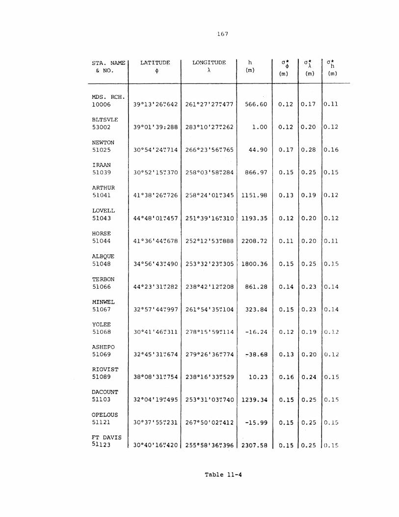
167

STA. NAME LATITUDE LONGITUDE h a* a* a* 4J !.. h

& NO. cp X (rn) (rn) (rn) (rn)

MOS. RCH.

10006 39°13'26~642 261°27'27':477 566.60 0.12 0.17 0.11

BLTSVLE 53002 39°01'39:288 283°10'27~1 262 1.00 0.12 0.20 0.12

NEWTON 51025 30° 54 I 24 1:714 266°23 I 56 11765 44.90 0.17 0.28 0.16

IRAAN 51039 30°52 1 15 11370 258°03 I 58~1 284 866.97 0.15 0.25 0.15

ARTHUR 51041 41° 38' 26~1 726 258°24 I 01 ~1 345 1151.98 0.13 0.19 0.12

LOVELL 51043 44°48'01:.'457 251°39'16~310 1193.35 0.12 0.20 0.12

HORSE 51044 41°36'44 11678 252°12 '53~1 888 2208.72 0.11 0.20 0.11

ALB QUE 51048 34°56 1 43 11490 253°32'23'1305 1800.36 0.15 0.25 0.15

TERBON 51066 44°23 I 31 1•1 282 238°42 '12'1208 861.28 0.14 0.23 0.14

MINWEL 51067 32°57'44~1 997 261°54'35'.'104 323.84 0.15 0.23 0.14

YO LEE 51068 30°41'46'.'311 278°15' 59~1 114 -16.24 0.12 0.19 0.12

ASHEPO 51069 32°45'31'.'674 279°26' 36~1 774 ~38.68 0.13 0.20 0.12

RIOVIST 51089 38°08'31'.'754 238°16'33'.'529 10.23 0.16 0.24 0.15

DACOUNT 51103 32°04 I 1911495 253°31'03'.'740 1239.34 0.15 0.25 0.15

OPELOUS 51121 30°37' 55~'231 267° SQ I 02 ~'412 -15.99 0.15 0.25 O.Ei

FT DAVIS 51123 30°40 I 16~'420 255°58'36'.'396 2307.58 0.15 0.25 0.15

Table 11-4

168

STA. NAME LATITUDE LONGITUDE h o* o* o* <I> A h & NO. <I> A (m)

(m) (m) (m)

PILLPT 10055 37°29'53~123 237°30'04':985 13.51 0.15 0.25 0.15

CASH 10021 37°33'06~952 273°55 I 09':742 229.40 0.19 0.29 0.17

UKAMISS 10022 34°4 7' 15':796 271 °45'29'! 375 211.70 0.26 0.41 0.22

TERMISS 10023 33°33' 54':992 270°50'03':480 103.60 0.20 0.30 0.18

OXALIS 53063 36°54'50~743 239°26'44':530 -1.44 0.14 0.22 0.13

a = 6378145.0 1/f = 298.25

NOTE: o<l>, oA, oh were not given for stations 4, 18, 15, 16, 17. The

values given here are the means of the values o<l>, oA, oh of

all other 15 stations.

* o<l>, o>.' oh represent the internal accuracy of the solution.

TABLE 11-4 (cont'd)

DOPPLER COORDINATES COINCIDENT 1-HTH TRANSCONTINENTAL

TRAVERSE POINTS

1.6<)

STA. NAI\'!E lJ\TI1'UDE !.ON(; T 'Pll DJ·: (l II ll N (l

</> II (m)

II & NO. </> A (m)

(m) (m) =ll

(mf

MDS. RCH. 10006 39°13 I 26~686 261°27 1 29 1.'494 0.0 599.40 0.0 0.0 0.0

BLTSVLE 53002 39°01 1 39~261 283°10 1 26 1.'899 3.0 42.80 0.3 -2.7 5.9

NEWTON 51025 30°54 I 24 1:080 266°23 1 57~134 2.0 85.70 0.2 2.1 3.9.

IRAAN 51039 30°52 1 14~847 258°04 1 00~426 2.0 898.90 0.2 0.6 3.8

ARTHUR 51041 41° )fl 1 ?.7~'013 25!1°24 1 03~844 1.0 1179.40 0.1 4.6 2.2

LOVELL 51043 44°48 1 02~1 028 251 °39 1 19~'733 2.0 1213.55 0.2 6.8 3.9

HORSE 51044 41°36 1 56~'136 252°12 1 57'.'024 1.8 2231.30 0.2 5.2 3.4

TERBON 51066 44°23 1 32~'167 238°42 1 17~'070 3.1 891.30 0.3 -16.4 6.1

ALBQUE 51048 34°56 1 43~'351 253°32 1 25~1 929 1.8 1829.60 0.2 0.5 3.5

MINWEL 51067 32°57'44%02 261 O 54 I 36': 968 1.6 359.60 0.2 -2.0 3.1

YULEE 51068 30°41 '45'.'626 278°15 1 59'.'246 3.0 17.00 0.3 4.4 5.7

ASHE PO 51069 32°45'31~'194 279°26 1 36'.'789 2.9 2.20 0.3 -0.3 5.6

RIOUIST 51089 38°08' 32'.' 353 238°16 1 37'.'829 3.2 51.80 0.3 -30.7 6.2

DACOUNT 51103 32°04 1 19'.'097 253°31 1 06~299 2.1 1271.60 0.2 -3.5 4.0

OPELOUS 51121 30° 37 I 54~~ 595 267°50 I 05~'405 2.2 19.50 0.2 3.1 4.1

FT. DAVIS 51123 30°40 1 15'.'872 255°58 1 44:120 2.1 2065.60 0.2 1.1 4.0

':P~h1e 11-5

170

STA. NAME LATITUDE LONGITUDE acp H OH N a H

& NO. cp (m)

(m) (m)

(m) cp A

(mf

PILLPT 1005(, 37°29 1 53 1.'441 237 ° \0 I 09'.'749 3.3 53.82 0.3 -32.8 6.4

CASH 10021 37°33 1 06'.'818 273° 55 I 10'.' 341 2.1 267.00 0.2 -1.4 4.1

UKAMISS 10022 34°47 I 15 1.'482 271°45 I 30~1 184 2.0 247.10 0.2 3.3 4.0

TERMISS 10023 33°33'54~598 270° 50 I 04 '.'408 2.1 138.60 0.2 4.0

OXALIS 53063 36°54'51 1.'184 239° 26'48'.'612 3.1 40.08 0.3 -30.4 6.0

a = 6378206.4 1/f 294.98525

*STN. MDS RCH. (10006) IS THE TERRESTRIAL NETWORK INITIAL POINT

TABLE 11-5 (cont 1 d)

U.S.A. TRANSCONTINENTAL TRAVERSE COORDINATES

/:;. 51066

/:;. 51043

.t. 51044

.t..51048

651041

6 MDS RCH 10006

651067

D. 51039 51025.t..

Figure 11- 2

530026

.t..10021

610022

610023

Twenty- one Doppler Tracking Stations in the United States of America

1-' ._J

1-'

172

2 2 2 [Beuglass, 1974] were added to each of o$, oA, ·oh for each station

to yield realistic varianCl'S for th~ Doppler coordinates with

respect to their coordinate system.

No estimates of the accuracy of the Transcontinental

Traverse coordinates ($, A) were given since they represent prelim-

inary results [Strange, 1975]. In lieu of this, the rule of thumb

[NASA, 1973]

2/3 oA = 0.020 K m (11- 1)

was used, where K is the distance of ($, A) from the terrestrial

initial point. In this test, (o$ , oA ) have been assumed to be k k

equal to zero, although as explained previously (1.3), this need not

be the case.

Similarly, no accuracy estimates were given for either H

or N. Again, some rules of thumb were adopted to have some standard

deviations. Assuming that all heights were determined by spirit

levelling, the relationship [NASA, 1973]

a = 1.8 K2/ 3 . 10-3 m H

(U- 5)

was used. For N, assuming that astrogeodetic methods had been used,

oN was approximated by [Badekas, 1969]

(11-6)

In this test, the ellipsoidal height (hk = Hk + Nk) at the terrestrial

network {nitial point has been assumed to have oh = 0. Again, this

will most likely not be the case in practice (1.3).

The Doppler network coordinates are referred to system l in

the Bursa model (7.1), while the Transcontinental Traverse is related

173

to system 2. Since the Doppler coordinates were given in terms of

geodetic coordinates {~, A, h), they, and their variance-covariance

matrix, were transformed to a Cartesian coordinate system using {1-2)

and {2-3) respectively. The Transcontinental Traverse {terrestrial)

coordinates were expressed in terms of{~, A, H, N), and they too

were transformed to a Geodetic Cartesian system using the procedure

outlined in 2.1.3. The semi-major axes and flattenings of the two

ellipsoids involved are given in Tables 11-4 and 11-5.

Four test runs were made u~ing the data described. The

resulting transformation parameters are given in Table ll-6. In

all cases, the x2 analysis of variance failed at the 95% confidence

level. Although no indepth analysis of the reasons for the failures

could be carried out, it is the author's opinion that the approximate

method by which variances were generated for the terrestrial coordi­

nates was the major problem. This is particularly evident for Test

#3 (Table ll-6) in which all transformation parameters were

significant. The other reason, which is of greater consequence, is

that the model {Bursa) is not suitable for the combination of

terrestrial and satellite networks.

A brief examination of the results of Tests #1 and #2

(Table 11-6) shows that the rotation parameters generated are all

insignificant. In all tests, the translation components are signif­

icant, and Tests #1 and #3 show the scale difference to be of

significant magnitude.

In comparing the results reported here with those of

Strange et al. [1975), it was found that the translation components

174

Test #1

X = -22.6 m !l == 6.3 m ' = 0~'10 0 = 0~'29 0 X )( l"

0 X

Yo = 154.4 m 0 = 5.8 m ,. = 0~'02 (J = 0'.'16 yo y L

y z = 172.6 m a = 7.3 m r = 0~'10 a = 0':17 K=l.l ppm 0 =0.4 ppm

0 z z £ K 0 z

2 1.00 df 56

A2 0.54 0 = = a

0 0

Test #2

X = -22.7 m 0 = 6.3 m E: = 0'.'07 0 = 0~'29 0 X X E:

0 X

Yo = 150.0 m 0 = 5.5 m E: = 0':03 0 = 0':16 Yo y E: y

z = 177.6 m CJ = 7.0 m E: = 0'.'12 CJ = 0'.'17 K: eliminated from 0 z z E:

the solution. 0 z 2

1.00 df 57 A2

0.64 a = = CJ = 0 0

Test ·#3

X = -25.3 m 0 = 0.8 m E: : 0 X X

eliminated 0

Yo = 156.6 m a = 2.1 m E: : from the yo y

solution K = 1.1 ppm 0 = 0.4 ppm K z = 174.8 m a = 1.9 m E: :

0 z z 0

2 1.00 df 59

A2 0.52 a = = a =

0 0

Test #4

X = -26.0 m 0 = 0.7 m E: : 0 X X eliminated

0 from the

yo = 151.7 m 0 - 0.7 m E: : . Yo y solution K: eliminated from the

solution z = 179.1 m a = 0.7 m E: : 0 z z

0

2 1. 00 df 60

A2 0.62 a = = 0 =

0 0

TABLE 11-6

BURSA MODEL TESTS

COMBINATION OF A DOPPLER AND A TERRESTRIAL NETWORK

175

(Test #1, Table ll-6) agreed to within 2 m in all three components.

The scale difference of 1.1 ppm compares favourably with the 1.0

ppm. However, Strange et al. [1975] found significant rotations

£ (-0~10, a= 0~04) and£ (0~19, a= 0~04). This latter difference y z

is most likely due to the somewhat different data used and the

different variances attributed to the terrestrial coordinates.

For each test run, the adjusted coordinates of each net-

work and their variance-covarinace matrices were computed. In

all cases, there was a significant decrease in the standard devia-

tions of the terrestrial coordinates. For example, before the net-

work combination, the standard deviations of the Cartesian

coordinates of point 51068 (YULEE) were 3.06 m, 5.11 m, and 3.89 m

in the x, y, and z components respectively. After the combination

they were 0.69 m, 0.36 m, and 0.36 m. There was little change in

the standard deviations of the Doppler coordinates.

There were significant changes in the terrestrial coordi-

nate values in all tests. For example, the adjusted terrestrial

coordinates for Test #4 experienced changes of -2.77 m to 2.76 min

x, -2.54 m to 4.01 min y, and -3.70 m to 0.39 min z. There were

no changes greater than + 0.2 m (Test #4) in any Doppler

coordinates.

Comparisons of the Bursa model results with those of the

Veis and Molodensky are given in 11.3.

176

11.2 Veis and Molodensky Models

These models have been used in some studies in which the

combination of terrestrial and satclli.te networks were carried out

[e.g. Badekas, 1969; Mueller and Kumar; 1975). The test computations

reported herein have been carried out solely for the purposes of

comparison with results generated via the Bursa model.

The Doppler and terrestrial data used is given in Tables

11-4 and 11-5 respectively. Five test runs were made, each of which

contained different sets of unknown parameters. The resulting

translation components and network scale and orientation parameters

are given in Table 11-7.

None of the test runs were acceptable on the basis of a x2

analysis of variance at 95%. One of the reasons for this, as stated

regarding the Bursa model test, is most probably the approximate

methods by which terrestrial coordinate variances were generated.

The fact can not be discounted, however, that the failure of the

x2 analysis of variance is an indication that the Veis (or Molodensky)

model is not adequate for the combination of terrestrial and

satellite networks.

In all five test computations, only the translation com­

ponents and scale difference were found to be significant. As with

the Bursa model tests, there was little change in the Doppler

coordinates or their associated variances. Significant changes in

terrestrial coordinates and their variances occurred as a result of

the Veis (or Mo1odensky) combination procedure.

Comparisons of the results generated for this report could

177

Test #1

X = -26.2 m a = 0.7 m dA = -0.04 adA = 0'.'09 0 X

0

Yo = 151.2 m a = 0.7 m dll = -0'.'09 adll = 0~'29 Yo

z = 179.3 m a = 0.7 m dv = -0'.'10 0 dv = 0'.'20 K=l.l ppm a =0.4 ppm

0 z K 0

Molodensky Rotations:

1/Jx = 0'.'10 1/Jy = 0~'02 ljJZ = 0'.'10

2 1.00 df 56

A2 0.54 0 = = a =

0 0

Test #2

X = -26.1 m a = 0.7 m dA = -0'.'04 adA = 0~'09 0 X

0

Yo = 151.8 m a = 0.7 m dll = .,.0~'06 0d11 = 0'.'29

Yo z = 179.2 m a = 0.7 m dv = -0'.'12 adv = 0'.'20 K: eliminated from

0 z the solution 0

Molodensky Rotations:

1/Jx = 0~'07 1/Jy = 0'.'03 ljiz = 0'.'12

2 1.00 df 57

A2 0.64 a = = a =

0 0

Test #3

X = -26.1 m a = 0.7 m dA: eliminated 0 X.

from the 0

yo = 151.2 m a = 0.7 m d\1: solution Yo

z = 179.3 m a = 0.7 m dv: K=1.1 ppm a =0.4 ppm ·o z K 0

2 1.00 df a = = 59

A2 a = 0.52

0 0

Table 11-7

178

Test #4

X -26.0 rn 0 0.7 m dA: eliminated 0 X

0 from the

Yo 151.7 m 0 0.7 m dp: solution yo

z 179.1 m () 0.7 m dv: K: eliminated from the 0 7. solution 0

2 1.00 df 60

~2

0.62 a a 0 0

Test #5

X -26.1 rn a 0.7 rn dA = -0'.'04 adA = 0'.'09 0 X

0

Yo 151.2 rn a 0.7 m d~: eliminated from yo the solution

z 179.3 m a 0.7 m dv: K=l.l ppm a =0.4 ppm 0 z K

0

Molodensky Rotations:

ljJ = -0'!02 ljly = -0'.'03 i)lz = 0'.'02 X

2 ·2 0 = 1.00 df = 58 (J = 0.53

0 0

TABLE 11-7 (cont'd)

VEIS AND MOLODENSKY MODEL TESTS

COMBINATION OF A TERRESTRIAL AND A DOPPLER NETWORK

179

not be compared with those of other investigators. The reason for

this is that no outside investigators have attempted to combine the

u.s. Transcontinental Traverse and Doppler networks using either a

Veis or a Molodensky model.

11.3 Comparison of Results

In 7.4, it was shown that the Bursa and Veis (or Molodensky)

models are not mathematically equivalent. This was brought to light

in a comparison of the treatment of a terrestrial initial point in

the formulation of each of the models, and in a comparison of the

elements of the design matrices A. in the estimation procedure. As 1

has been shown in other investigations, the models can be made to

be equivalent under certain conditions concerning the terrestrial

initial point and the formulation of the mathematical models

[Krakiwsky and Thomson, 1974; Mueller and Kumar, 1975].

A comparison of the test results generated using the same

data in each of the models helps to further illustrate the differences

in the models. In each of Tests #l and #2 (Tables 11-6 and ll-7),

the translation components of the Bursa model solution are different

from those of the Veis (or Molodensky) model solution, while the

scale difference parameters and rotation parameters are equivalent

numerically. The latter is easily understood. Since there is only

one set of rotation parameters and one scale difference parameter in

each model all rotation and scale errors, whether they are the result

of discordant, mis-scaled coordinate systems or misoriented mis-scaled

180

networks, are represented by these parameters. The results of Tests

#3 (Tables 11-6 and 11-7), from which all orientation parameters

were eliminated, show that the two sets of translation components

(Bursa and Veis or Molodensky) are still significantly different -

0.8 m in x , 5.4 m in y , and -4.5 m in z . The scale difference 0 0 0

parameters are, however, equivalent. Only in T~st #4 of each

model, in which all rotation and scale parameters have been

eliminated from each solution, are the results (translation components)

equivalent.

12. RECENT THREE-DIMENSIONAL MODELS - UNKNOWN DATUM TRANSFORMATION

PARAMETERS

Each of the three models in this category - Hotine, Krakiwsky­

Thomson, and Vanicek~Wells - contain two sets of unknown rotation

parameters. The separation of the two sets of rotations in the former

two models is achieved via a specific least-squares estimation procedure,

while the latter involves several terrestrial networks in a single

parametric least-squares solution. In all three instances, final

conclusions regarding the validity and usefulness of the models will

only be possible when the proper data is available for numerical testing.

Proper data is considered to be two or more sets of terrestrial and

satellite network coordinates that are the result of rigorous but sep­

arate network computation procedures. Unfortunately, this type of data

is not readily available at present. Thus, the tests carried out

merely indicate that the models proposed, and their methods of solution,

are feasible.

Contained herein are test results of the combination of a

Doppler and a terrestrial network using the Krakiwsky-Thomson model.

181

182

The Vanicek-Wells model was not tested for this report.

Te~t results for this model have been reported elsewhere [Wells and

vanicek, 1975].

12•1 Krakiwsky-Thomson Model

The data given in 11.1 (Tables 11- 4 and 11- 5 ) was used to

geperate some test results for the combination of a Doppler and a ' .

terrestrial network. The estimation procedure outlined in 8.2 was :

utilized.

Three sets of results are given in Table 12-1. 2

Based on a X

analysis of variance at 95%, none of the results were accepted. Several

assumptions may be made regarding this, none of which can be investi-

gated at present. The data used was not complete. There was no

. covariance information amongst and between the Doppler coordinates. The

variances of the terrestrial coordinates were generated using some rules

of thumb (11.1), and therefore there was no covariance amongst and

between coordinates. Of course, there is the possibility that the model

and/or the estimation procedure may be inadequate. However, with the data

used, no conclusive evidence of this could be deduced.

As required for the estimation procedure, the observables

(network coordinates) were split into two parts (inner and outer zones).

The inner zone consisted of 5 points that were all with' 1000 km of the

terrestrial network initial point. The remaining observables (Doppler

183

Test #l

Datum Transformation Parameters

X -25.1 m a 6.5 m L -0'.'01 (J 0~53 0 X X t:

0 X

yo 152.2 m a 10.3 m E 0~'29 a 0~'22

yo y E y

z 180.6 m a 12.8 m E "' -0~'1 g 0 0~21 0 z z E

0 z

Network Parameters

dA -0'.'25 adA 0~'28

d\1 -0'.'18 ad\1 0~'64

dv -0'.'30 adv 0~23 K == 1.1 ppm (J -.5 ppm .K

Molodensky Network Rotations

1); 0~'18 tlJY -0~'03 '. tlJZ 0~'39 X

2 1.00 df 53

A2 0.46 a a

0 0

Test #2

Datum Transformation Parameters

X -30.6 m a 5.0 m E : eliminated 0 X X

from the 0

yo 152.0 m a 1.0 m E : solution yo y

z 179.3 m a 0.7 m E ==-0:.'18 (J 0:.'21 0 z z E

Network 0 z

Parameters

dA 0'.'01 adA 0~'21

d\1 -0'.'21 ad\1 0'.'35

dv -0~'34 adv == 0:"23 K == 1.1 ppm a 0.5 ppm K

Mo1odensky Network Rotations

1/J 0~'24 t~Jy 0~'18 t~Jz 0~'26 X

2 1.00 df 55

~2

a = a 0.47 0 0

TABLE 12-1

184

Test #3

Datum Transformation Parameters

X -26.2 m a 0

yo 151.3 m a

z 179.3 m a 0

= X

0

yo

z 0

0.7 m

0.7 m

0. 7 m

Ex eliminated from the solution

£ y

£ z

Network Parameters

dA

dll

dv

ljix =

2 (J

0

-0~'12 a = dA

0'.'10

eliminated from the solution

K = 1.2 ppm a = 0.5 ppm K

Molodensky Network Rotations

-0~'01 ljiy -0~'09 1/J 0~'07 z

1.00 df 58 ~2

0.50 ao

TABLE 12-1 (cont'd)

TEST RESULTS OF THE KRAKIWSKY-THOMSON MODEL

185

and terrestrial coordinates of 16 points) were in the outer zone. This

split was purely arbitrary since, due to a lack of sufficient data, no

conclusive testing could be carried out regarding the optimal separa-

tion of observables.

In all three sets of test results (Table 12-1), the system

and network rotation parameters were insignificant. Attempts to

isolate significant rotations, such as longitudinal (£ ) system z

rotation (Table 12-l, Test #2) and an azimuthal (dA) network rotation

(Table 12-1, Test #3) did not improve the solution. Only the datum

translation components (x , ~ , z l and the network scale difference 0 0 0

(K) proved to be significant.

It should be noted that the network rotations determined

are expressed in three ways. The Krakiwsky-Thomson model developed

herein is in terms of Veis-type network rotations. As pointed out in

7.3, Molodensky-type network rotations are easily computed from

these.

As expected, the variances of the terrestrial network

coordinates improved (decreased) as a result of the combination pro-

cedure. Changes in the terrestrial coordinates of up to 2.8 in x,

3.3 min y, and 3.5 min z took place. All Doppler coordinates

changed by 0.2 m or less.

No further analysis was carried out. As indicated;earlier,

the lack of data was a major problem and hindered adequate testing.

186

SECTION V

CONCLUSIONS AND RECOMMENDATIONS

13. CONCLUSIONS AND RECOMMENDATIONS

As a result of the research ~nd analyses carried out for

this study, the following conclusions have been arrived at:

1. No matter what methodology is used to establish a datum for

terrestrial geodetic networks, the quantities and procedures used

must be stated clearly and explicitly. Assuming that the practice

of using a reference ellipsoid as a horizontal network datum will

be continued, it should be remembered that it is a three-dimensional

object and must be positioned and oriented as such in the earth

body. This means that the conditions for parallelity of

axes must be applied at the terrestrial network initial

point. Further, the manner by which the initial point geodetic

coordinates are obtained must be clearly defined. Only then will

the rigorous propagation of errors, into appropriate quantities,

be possible.

All of the information mentioned above is essential for

a total understanding of how a particular datum has been chosen,

positioned, and oriented. This will be particularly crucial, for

example, for an in depth analysis of the preliminary results of the

redefined Canadian geodetic networks.

187

188

2. Precise and homogeneous satellite networks, such as the Canadian

Doppler network, contain errors that are of a lower order of

magnitude than those that could be expected in a terrestrial net­

work of similar extent. Such networks can provide essential

information for:

(i) the establishment of a terrestrial datum;

(ii) the modelling of systematic errors in terrestrial networks;

(iii) the establishment of a homogeneous, three-dimensional,

terrestrial geodetic network.

3. To utilize a maximum amount of satellite network data with the

least amount of computational effort in the adjustment of terres­

trial network, the use of satellite network coordinates as

weighted parameters is the most practical. The basic disadvantages

of this type of approach are that:

(i) the datum transformation parameters must be known;

(ii) unmodelled systematic errors will affect the solution and

residual vectors.

4. Three dimensional models for the combination of satellite and

terrestrial geodetic networks are preferable. The advantages are:

{i) nj loss of covariance information such as when the data is

split into horizontal (~, A) and vertical (h) components;

{ii) datum transformation parameters can be solved for rigorously;

(iii) the overall effects of systematic errors in the terrestrial

network can be modelled;

(iv) given sufficient terrestrial data, the orientation of the

satellite and terrestrial datums with respect to Average

Terrestrial axes can be determined.

189

Arguments regarding the insignificance of correlation

between (~, A) and (h) components in networks such as the Canadian

Doppler can not be assumed, particularly on a continental basis.

5. The Bursa and Veis (or Molodensky) models are not mathematically

equivalent. Under certain conditions, they give equivalent

numerical results. None of these three models are considered to

adequately model the unknowns in the combination of terrestrial

and satellite networks.

6. The Bursa model is adequate for the combination of two or more

satellite networks.

7. The Krakiwsky-Thomson and Hotine models reflect more

adequately than the other models the real physical situation .

that exists when combining a satellite and a terrestrial

network.

8. The Vanicek-Wells model is the only model that relates the orienta­

tion of the axes of a satellite datum and those of several

terrestrial datums to the Average Terrestrial coordinate system.

9. Theoretically, a combination of the Krakiwsky-Thomson and Vanicek­

Wells models can be used to combine several terrestrial datums and

their related networks and a satellite datum and its network. Such

a procedure will yield the orientations of each datum with

respect to one another and the Average Terrestrial coordinate

system, the position of each datum with respect to the other, and

a parameterization of the overall effects of systematic scale and

orientation errors in each terrestrial network.

This study has led to four recommendations that, in the

190

author's opinion, are important in the Redefinition of the North

American geodetic networks.

1. The North American Densification of the Worldwide Satellite

Triangulation (BC-4) Network should be investigated, once sufficient

terrestrial survey ties become available, with respect to the

Canadian and U.S. Doppler Networks. Such an investigation should

lead to the eventual use of this data in the redefinition of the

North American geodetic networks.

2. The Krakiwsky-Thomson model should be fully tested when adequate

data becomes available. The data should consist of:

(i) the complete definitions of the terrestrial and satellite

datums;

(ii) the coordinates and associated variance-covariance matrix of

a homogeneous satellite network, such as that of the

completed Canadian Doppler network;

(iii) the coordinates and associated variance-covariance matrix of

a readjusted, homogeneous, three-dimensional terrestrial

network with several hundred network points common to those

in (ii) above;

or

The readjusted horizontal (4>, A) and vertical (H) network

coordinates and associated variance-covariance matrices,

plus the geoidal heights (N) and associated variance­

covariance matrix with several hundred network points

common to those in (ii) above.

3. Serious consideration should be given to the three-dimensional

191

combination of the satellite (Doppler, BC-4) and readjusted

terrestrial networks in the redefinition of the North American

geodetic networks. The several hundred network points involved

would form the basis of future three-dimensional networks.

4. There should be efforts made towards the rigorous establishment

of a three-dimensional terrestrial network in North America.

This will permit, in the future, an unadulterated use of inherently

three-dimensional information, such as that obtained via satellite

and inertial positioning.

192

REFERENCES

Anderle, Richard J., and Mark G. Tanenbaum (1974). Practical Realization of a Reference System for Earth Dynamics by Satellite Methods. NWL Technical Report, No. TR-3151. U.S. Naval Weapons Laboratory, Dahlgren, Virqinia.

Anderle, Richard J. (1974 (a)). Rule uf 1\rtificJal Satellites in Hcdefinitirm of the North American Datum. The Canadian Surveyor, Vol. 28, No. 5.

Anderle, Richard J. (l974(b)). Transformation of Terrestrial Survey Data to Doppler Satellite Datum. Journal of Geophysical Research, Vol. 79, No. 35.

Anderle, R.J. (1974(c)). Simultaneous Adjustment of Terrestrial Geodimeter and Satellite Doppler Observations for Geodetic Datum Definitions. NWL Technical Report TR-3129. U.S. Naval Weapons Laboratory.

Badekas, John (1969). Investigations Related to the Establishment of a World Geodetic System. Reports of the Department of Geodetic Science Report No. 124, The Ohio State University, Columbus.

Baker, Captain Leonard S. (1974). Geodetic Networks in the United States. The Canadian Surveyor, Vol. 28, No. 5.

Beauglass, L.K. (1974). Positions for 1973 Based on Doppler Satellite Observations. NWL Technical Report, No. TR-3181.

Baal, J.D. (1975). Private Communication with the author.

Bamford, G. (3rd. ed. 1971). Geodesy. Oxford University Press, London.

Brown, D.C. (1970) Near Term Prospects for Positional Accuracies of 0.1 to 1.0 Metres from Satellite Geodesy. DBA Systems, Incorporated, Melbourne, Florida.

Bursa, M. (1962). The Theory of the Determination of the Non parallelism of the Minor Axis of the Reference Ellipsoid, Polar Axis of Inertia of the Earth, and Initial Astronomical and Geodetic Meridians from Observations of Artificial Earth Satellites. Trans­lation from Geophysicaet Geodetica, No. 6.

Bursa, Milan (1967). On the Possibility of Determining the Rotating Elements of Geodetic Reference System on the Basis of Satellite Observations. Studia Geophysica et Geodaetica, No. 11

Chamberlain, C.C., D.B. Thomson and E.J. Krakiwsky (1976). A Study of Systematic Errors in Horizontal Geodetic Networks. Department of Surveying Engineering Contract Report, Geodetic Survey of Canada Contract No. OSU5-0ll9, University of New Brunswick, Fredericton.

Chovitz, Bernard (1974). Three-Dimensional Model Based on Hotine's "Mathematical Geodesy". The Canadian Surveyor, Vol. 28, No. 5.

193

Dracnp, J.F. (1975). Use of Doppler Positions to Control Classical Geodetic Networks. Presented to the International Association of Geodesy, International Union of Geodesy and Geophysics, XVI General Assembly, Grenoble, France.

Enin~ I.I. (1959). Main Systematic Errors in Precise Levelling. Bulletin Geodesique, No. 52.

Fubara, D.M.J. (1972). Three-Dimensional Adjustment of Terrestrial Geodetic Networks. The Canadian Surveyor, Vol. 26, No. 4.

Heiskanen, Weikko A., and Helmut Moritz (1967). Physical Geodesy. W.H. Freeman and Company, San Francisco.

Holdahl, s. (1974) Time and Heights. The Canadian Surveyor, Vol. 28, No. 5.

Hothem, Larry D. (1975). Evaluation of Precision and Error Sources Associated with Doppler Positioning. Presented at the 1975 Spring Annual Meeting of the American Geophysical Union, Washington, D.C.

Hotine, M. (1969). Mathematical Geodesy. ESSA Monograph No.2. u.s. Department of Commerce, Washington, D.C.

Hradilek, L. (1972). Refraction in Trigonometric and Three-Dimensional Terrestrial Networks. The Canadian Surveyor, Vol. 26, No. 1.

John; s. (1976). The Determination of the Astrogravimetric Doppler Satellite Geoidal Heights as Constraints. of Surveying Engineering, M.Sc. Thesis (in prep.). New Brunswick

Geoid Using Department University of

Jones, Harold E. (1971). Systematic Errors in Tellurometer and Geodimeter measurements. The Canadian Surveyor, Vol. 25, No. 4.

Jones, Harold E. (1973). Geodetic Datums in Canada. The Canadian Surveyor, Vol. 27, No. 3.

Kouba, J. (1970). Generalized Least Squares Expressions and MATLAN Programming. Department of Surveying Engineering, M.Sc. Thesis, University of New Brunswick, Fredericton.

Kouba, J. (1976(a)). Doppler Satellite Levelling. The Canadian Surveyor (to be published).

Kouba, J. (1975). Doppler Satellite Control in Establishing Geodetic Control Network. Contributions of the Earth Physics Branch, No. 34.

194

Kouba, J. and J.D. Boal (1975). Program GEODOP. Geodetic Survey of Canada, Ottawa.

Kouba, J. (1976(b)). Private communication with the author.

Krakiwsky, E.J. and I.I. Mueller (1966). Proposed Establishment of a First-Order Height System in the U.S.A. Presented at the 47th Annual Meeting of the American Geophysical Union, Washington, April 19-22.

Krakiwsky, E.J. and D.E. Wells (L971). Coordinate Systems in Geodesy. Department of Surveying Engineering, Lecture Notes No. 16, University of New Brunswick, Fredericton.

Krakiwsky, E.J. (1972). Three Dimensional Coordinates in Surveying. An Invited Paper to the Second Colloquium on Surveying and Mapping for the Petroleum Industry, Banff, May 24 to 26.

Krakiwsky, E.J. and D.B. Thomson (1974(a)). Geodetic Position Computations. Department of Surveying Engineering, Lecture Notes No. 39, University of New Brunswick, Fredericton.

Krakiwsky, E.J. and D.B. Thomson (1974(a)). Mathematical Models for the Combination of Terrestrial and Satellite Networks. The Canadian Surveyor, Vol. 28, No. 5.

Krakiwsky, E.J. (1975). A Synthesis of Recent Advances in the Least Squares Method. Department of Surveying Engineering ·Lecture Notes No. 42, University of New Brunswick, Fredericton.

Ku, L.F. (1970). The Evaluation of the Performance of Water Level Recording Instruments. Symposium on Coastal Geodesy, Munich, July.

Kukkamaki, T.J. (1949). On Lateral Refraction in Triangulation. Bulletin Geodesique, No. 11.

Kukkamaki, T.J. (1961). Lateral Refraction on the Sideward Slope. Annales Academiae Scientiarum Fennicae, Series A, III Geologica - Geographica, 61.

Lambeck, K. (1971). The Relation of Some Geodetic Datums to a Global Geocentric Reference System. Bulletin Geodesique No. 99.

Lennon, G.W. (1974). Mean Sea Level as a Reference for Geodetic Levelling. The Canadian Surveyor, Vol. 28, No. 5.

Lisitzin, E. and J.G. Pattulo (1961). The Principal Factors Influencing the Seasonal Oscillation of Sea-Level. Journal of Geophysical Research, Vol. 66, No. 3.

195

Marussi, Prof. Antonio (1974). Geodetic Networks in Space. The Canadian Surveyor, Vol. 28, No. 5.

Mather, R.S. (1974). Geodetic Coordinates in Four Dimensions. The Canadian Surveyor, Vol. 28, No. 5.

McLellan, C.D. (1974). Geodetic Networks in Canada. The Canadian Surveyor, Vol. 28, No. 5.

McLellan, D. (1973). Private communication with the author.

Meade, Buford K. (1967). High-Precision Geodimeter Traverse Surveys in the United States. Presented to the XIV General Assembly of IUGG, International Association of Geodesy, Lucero, Switzerland.

Meade, B.K. (1974). Doppler Data Versus Results from High Precision Traverse. The Canadian Surveyor, Vol. 28, No. 5.

Meade, B.K. (1975). Private communication with the author.

Merry, C.L. and P. Vanicek (1973). Horizontal Control and the Geoid in canada. The Canadian Surveyor, Vol. 27, No. 1.

Merry, Charles L. (1975). Studies Towards an Astrogravimetric Geoid for Canada. Department of Surveying Engineering, Technical Report No. 31, University of New Brunswick, Fredericton.

Molodensky, M., V. Yeremeyev, M. Yurkina (1962). Methods for Study of the External Gravitational Field and Figure of the Earth. Israel Program for Scientific Translations, Jerusalem.

Moritz, Helmut (1973). Stepwise and Sequential Collocation. Reports of the Department of Geodetic Science, Report No. 203, The Ohio State University, Columbus, Ohio.

Mueller, Ivan I. and John D. Rockie (1966). Gravimetric and Celestial Geodesy - A Glossary of Terms. Frederick Unger Publishing Co., New York.

Mueller, Ivan I. (1969). Spherical and Practical Astronomy as Applied to Geodesy. Frederick Unger Publishing Co., New York.

Mueller, I.I., C.R. Schwarz and J.P. Reilly (1970). Analysis of Geodetic Satellite (GEOS I) Observations in North America. Bulletin Geodesique No. 96.

Mueller, Ivan I. (1974(a)). Review of Problems Associated with Conventional Geodetic Datums. The Canadian Surveyor, Vol. 28, No. 5.

196

Mueller, I. I. (1974 (b)). eration Results. No·. 35.

Global Satellite Triangulation and .Trilat­Journal of Geophysical Research, Vol. 29,

Mueller, I.I. and M. Kumar (1975). The OSU 275 System of.Satellite Tracking Station Coordinates. Reports of the Department of Geodetic Science, Report No. 228. The Ohio State University, Columbus, Ohio.

NASA (3rd ed., 1973). NASA Directory of Observation Station Locations, Volumes·! and 2. Prepared by Computer Sciences Corporation, Falls Church, Virginia.

Nassar, M.M. and P. Vanicek (1975). Levelling and Gravity. Department of Surveying Engineering, Technical Report No. 33, Univer­sity of New Brunswick, Fredericton.

Paul, M.K. (1973). A Note on Computation of Geodetic Coordinates from Geocentric (Cartesian) Coordinates. Bulletin Geodesique No. 108.

Pope, A. (1975). The North American Densification Satellite Triangulation Network. Personal communication with the author.

Schmid, Hellmut H. (1965). Precision and Accuracy Consideration for the Execution of Geodetic Satellite Triangulation. The Use of Artificial Satellites for Geodesy, Volume II. Publication of the National Technical University, Athens, Greece.

Schmid, HellmutH. (1970). A World Survey Control System and Its Implications for National Control Networks. Papers of the 1970 Annual Meeting, Canadian Institute of Surveying.

Schmid, HellmutH. (1972). Status of Data Reduction and Analysis Methods for the Worldwide Geometric Satellite Triangulation Program.Geophysical Monograph 15, American Geophysical Union, Washington.

Schmid, Hellmut H. (1974). World Wide Geometric Satellite Triangulation. Journal of Geophysical Research, Vol. 79, No. 35.

Strange, W.E., L.D. Hothem, M.B. White (1975). Station Network in the United States.

The Satellite Doppler Presented to the

International Union of Geodesy and Geophysics, International Association of Geodesy, XVI General Assembly, Grenoble, France.

Strange, W. (1975). Private communication with the author.

Thomson, D.B. (1970). The Readjustment of Geodetic Networks in Eastern Canada. M.Sc. Thesis, Department of surveying Engineering, University of New Brunswick, Fredericton.

197

Thomson, D.B., M.M. Nassar, and C.L. Merry (1974). Distortions of Canadian Geodetic Networks due to the,Neglect of Deflections of the Vertical and Geoidal Heights. The Canadian Surveyor, Vol. 28, No. 5.

Thomson, D.B. and E.J. Krakiwsky (1975). Alternative Solutions to the Combination of Terrestrial and Satellite Geodetic Net­works. Contributions of the Earth Physics Branch, No. 45, Ottawa.

Thomson, D.B. and c. Chamberlain (1975). UNBSA- A Rigorous Computa­tion Procedure for Extensive Horizontal Geodetic Networks. Presented at the 68th Annual Meeting of the Canadian Institute of Surveying, Fredericton.

Tscherning, C.C. (1975). Determination of Datum-Shift Parameters Using Least Squares Collocation. Prese.nted at the 6th Symposium on Mathematical Geodesy, Siena, Italy.

Vanicek, Petr (1972). Physical Geodesy II. Department of Surveying Engineering, Lecture Notes No. 24, University of New Brunswick, Fredericton.

Vanicek, P., J.D. Boal, and T.A. Porter (1972). Proposals for a More Modern System of Heights for Canada. Department of Energy, Mines and Resources, Surveys and Mapping Branch, Technical Report No. 72-3.

Vanicek, P. and C.L. Merry (1973). Determination of the Geoid from Deflections of the Vertical Using a Least-Squares Surface Fitting Technique. Bulletin Geodesigue, No. 109.

Vanicek, P. and D.E. Wells (1974). Positioning of Geodetic Datums. The Canadian Surveyor, Vol. 28, No. 5.

Vanicek, P. (1975). Report on Geocentric and Geodetic Datums. Department of Surveying Engineering, Technical Report No. 32, University of New Brunswick, Fredericton.

Veis, G. (1960). Geodetic Uses of Artificial Satellites. Smithsonian Contributions to Astrophysics, Volume 3, Number 9. Smithsonian Institution, Washiugr.on.

Villasana, J. Alberto (1974). Geodetic Networks in Mexico. The Canadian Surveyor, Vol. 28, No. 5.

Vincenty, T. (1973). Three-Dimensional Adjustment of Geodetic Networks. DMAAC Geodetic Survey Squadron, F.E. Warren AFB, Wyoming.

Webster's New World Dictionary (1951). Nelson, Foster, & Scott Ltd., Toronto.

198

Wells, O.E. _(1974). Doppler Satellite Control. Department of Surveying Engineering, Technical Report No. 29, University of New Brunswick, Fredericton.

Wells, D.E., E.J. Krakiwsky and D.B. Thomson (1974). In.terrial and External Consistency of Doppler, Satellite Triangulation, and Terrestrial Networks. The Canadian Surveyor, Vol. 28, No. 5.

Wells, D.E. and P. Vanicek (1975). Alignment of Geodetic and Satellite Coordinate Systems to the Average Terrestrial System. Bulletin Geodesique No. 117.

Wolf, Helmut (1963). Geometric Connection and Re-Orientation of Three Dimensional Triangulation Nets. Bulletin Geodesiqlie, No. 68.