Columbia Program on Indian Economic

Policies

Working Paper No. 2011-5

Does Liberalization Promote Competition?

Laura Alfaro

Anusha Chari

Does Liberalization Promote Competition?

Laura Alfaro* Anusha Chari** Harvard & NBER UNC-Chapel Hill & NBER

October 2010

Abstract

Using firm-level data from India, this paper investigates the distributional effects of deregulation on firm size and profitability. The data suggest that average firm size declines significantly in industries that deregulated entry. Firm entry leads occurs from the left hand tail of the size distribution with more small firms entering the market while the largest incumbent firms get significantly bigger following deregulation. Quantile regressions show that the shift in the distribution of firm size is non-linear with average firm size increasing till around the 15th percentile, and then getting significantly smaller till the 90th percentile while the largest percentile (95%) gets significantly bigger over the sample period. The marginal entry of small firms is consistent with an increase in competition following entry deregulation. Consistent with a decline in monopoly power, the Herfindahl index of firm sales also shows a significant decline. While summary statistics suggest a decline in average firm profits, quantile regressions show significant non-linearity and a heterogeneous impact of deregulation on profitability.

*Laura Alfaro, Harvard Business School, Morgan 263, Boston MA, 02163, U.S.A. (e-mail: lalfaro@hbs.edu). **Anusha Chari, Department of Economics, CB #3305, University of North Carolina at Chapel Hill, Chapel Hill NC 27599, U.S.A. (email:achari@unc.edu). We thank Arvind Panagariya, Jagdish Bhagwati, Rajeev Dehejia, and all the participants at the Columbia University India workshop for helpful comments and suggestions. Work on this paper has been supported by Columbia University’s Program on Indian Economic Policies, funded by a generous grant from the John Templeton Foundation. The opinions expressed in the paper are those of the authors and do not necessarily reflect the views of the John Templeton Foundation.

2  

1. Introduction

The regulation of entry in an industry determines both the entry costs faced by firms, and

the degree of competition between firms (Blanchard and Giavazzi, 2003). The transition from a

regulated to deregulated environment may imply the decline of incumbent firms as entry costs

(regulatory) decline and new firms enter the market alternatively, while new firms enter the

market, large incumbents may be in a position to consolidate their positions further if the size of

the market expands. The deregulation of entry can therefore reduce and redistribute rents leading

to new distributions of firms within industries over time.

Recent research predicts that the deregulation of firm entry in will lead to (i) more firms

and less incumbent power (Blanchard and Giavazzi, 2003, Alesina et al., 2005); (ii) increases in

average firm size and profits through trade liberalization (Melitz and Ottaviano, 2008); (iii)

increasing dispersion in sales, assets, profits, (Campbell and Hopenhayn, 2005; Syverssen,

2004), and (iv) increasing turnover and firm age distributions tilting towards younger firms

(Asplund and Nocke, 2003). 1

In this paper we ask whether liberalization promotes competition. We employ firm-level

financial statement information from the manufacturing sector to examine the question in the

context of the massive deregulation that has taken place in India since 1991. The goal is to

investigate the distributional effects of deregulation on firm size and profitability. We define

deregulation broadly to include both domestic and foreign entry through FDI and trade.

A previous paper, Alfaro and Chari (2010a), examines the evolution of India’s industrial

composition between 1988-2005 by focusing on the micro-foundations of its productive structure

across industrial sectors, by ownership within sectors, and across time. The evidence shows great

dynamism by foreign and private firms in terms of growth in average numbers, assets, sales &

profits. However, the data suggest an economy still dominated by the incumbents (state-owned

firms and old private firms) in the form of continuing incumbent control in shares of assets, sales

& profits accounted for by state-owned & old private firms. Sectors dominated by state-owned

and old private firms before liberalization (with shares higher than 50%); incumbents remain the

dominant ownership group following liberalization.

The major exception to the pattern of incumbent firm dominance is seen in the average

growth of private firms in the services industries between 2001 and 2005. Asset, sales & profit                                                             

1 A monopolistic competition assumption in the goods market determines the size of rents.

3  

shares of private firms in business and IT services, communications services and media, health

and other services show a substantial increase in growth and in shares over this period. In this

paper we investigate the distributional impact of deregulation on firm size and profitability in

greater detail.

Melitz and Ottaviano (2008) provide a useful benchmark to fix ideas and motivate the

empirical analysis in the paper. In the Melitz-Ottaviano model, deregulation leads to bigger

markets and more competition. Tougher selection in the competitive markets following

deregulation implies higher average productivity and lower prices. In a key distinction from

Melitz (2003), market size induces important changes in the equilibrium distribution of firms and

their performance measures. The model’s predictions for the effects of bilateral trade

liberalization are very similar to those emphasized in Melitz (2003) in that trade forces the least

productive firms to exit and reallocates market shares towards more productive exporting firms.

Firms with lower productivity only serve their domestic markets. The parameterization on cost

draws is such that average firm size (output, sales) and profits higher in larger markets. Profits

increase because direct market size effect outweighs indirect effect through lower prices and

markups.

In the context of India, we can think of deregulation as increasing market size through

trade liberalization and FDI and domestic entry deregulation. An increase in competition may be

measured in several ways. Deregulating entry may imply an increase in dispersion in firm size

distributions, a reduction in concentration ratios or a decline in average firm size. Similar

measures can be applied to firm profitability.

A challenge we however face in this context is that in Melitz and Ottaviano (2008),

average profits and sales increase by the same proportion when market size increases through

trade. Thus, average industry profitability does not vary with market size and makes measuring

redistribution effects tricky. Furthermore, the period of deregulation in the early 1990s in India

coincides with rapid economic growth. Therefore, a dynamic model is better suited to examining

the effects of deregulation on competition against the backdrop of a growing economy.

We use firm-level data from the Prowess database collected by the Centre for

Monitoring the Indian Economy from company balance sheets and income statements. Prowess

covers both publicly-listed and unlisted firms from a wide cross-section of manufacturing,

services, utilities, and financial industries from 1989 until 2005. About one-third of the firms in

4  

Prowess are publicly-listed firms. The companies covered account for more than 70% of

industrial output, 75% of corporate taxes, and more than 95% of excise taxes collected by the

Government of India (Centre for Monitoring the Indian Economy). Prowess covers firms in the

organized sector, which refers to registered companies that submit financial statements.2

The main advantage of firm-level data is that detailed balance sheet and ownership

information permit an investigation of a range of variables such as sales, profitability, and assets

for an average of more than 10,800 firms across our sample period (1989-2005). We focus on

firms are classified across 62 3-digit industries in the manufacturing sector.3 The data are also

classified by incorporation year so that distinctions can be made across firms by age.4 As a

result, the data contain rich detail to characterize changes in firm size distributions, as well as

differentiate across types of firms such as incumbents and new entrants.

Our main results are as follows. First, average firm size declines significantly in

industries that deregulated entry (domestic, foreign) consistent with small firm entry combined

with import competition. Second, firm entry leads occurs from the left hand tail of the size

distribution with more small firms entering the market while the largest incumbent firms get

significantly bigger following deregulation. Third, quantile regressions show that the shift in the

distribution of firm size is non-linear with average firm size increasing till around the 15th

percentile, and then getting significantly smaller till the 90th percentile while the largest

percentile (95%) gets significantly bigger over the same time period.

The marginal entry of small firms is consistent with an increase in competition following

entry deregulation. The finding is consistent with Blanchard and Giavazzi (2003) as is the

reduction in average firm size implying less monopoly power. However, the increase in the size

of the very largest firms is consistent with the prediction from Melitz (2003) as large firms are

more likely to be exporters. Dispersion in firm size also increases consistent with Melitz and

Ottaviano (2008).

Consistent with a decline in monopoly power, the Herfindahl index of firm sales also

shows a significant decline. While summary statistics suggest a decline in average firm profits,

                                                            2 Section 3 describes in detail the advantages and shortcomings of the dataset. 3 As Goldberg et al. (2009) note, unlike the Annual Survey of Industries (ASI), the Prowess data is a panel of firms, rather than a repeated cross-section, and therefore, particularly well suited for understanding how firms adjust over time and how their responses may be related to policy changes. 4Although the liberalization process has been gradual, this does not preclude the analysis of the effects of reducing these constraints on the evolution of the firm-size distributions and profitability.

5  

quantile regressions once again show significant non-linearity and a heterogeneous impact of

deregulation on profitability.

We estimate a number of specifications to ensure the robustness of the findings. The firm

size regressions are estimated for both assets and sales. We use a balanced panel of incumbent

firms with and without fixed effects. The fixed effects specification controls for unobserved

heterogeneity at the firm-level. We use an unbalanced panel of firms to allow for entry and to

examine the distributional impact of deregulation. The specifications include a year trend

variable to control for the overall growth in the economy. Finally, standard errors are clustered at

the 3-digit NIC3 level to allow for correlations in residuals across firms within an industry.

The paper is organized as follows. Section 2 provides a brief survey of recent theoretical

models of deregulation that provide testable implications for our study. Section 3 describes the

data and Section 4 presents summary statistics about firm size distributions and profitability

before and after deregulation, and by incumbent and new entrant status. Section 5 presents the

empirical methodology and results. Section 6 concludes.

2. Predictions from Theory

Blanchard and Giavazzi (2003) and Alesina et al. (2005) are examples of models from

the macroeconomic literature on deregulation in product markets. Both models assume a

monopolistic competitive environment in which each firm produces a differentiated product with

capital and labor. In this setting, the elasticity of demand, ε, varies inversely with the degree of

product market regulation: tighter regulation is associated with a lower elasticity. One way to

rationalize this is to assume that the elasticity of demand is an increasing function of the number

of firms, m. Hence, ε = g(m), where g (·) > 0.

Blanchard and Giavazzi (2005) divide time in two periods, a short run, where the number

of firms is given, and a long run, where the number of firms is endogenous, determined by an

entry condition. They assume that firms face a cost of entry equal to c, which comes from

product market regulation. In the model, c is a shadow cost designed to motivate the focus on

regulation such that many regulatory barriers to entry take the form of legal and administrative

restrictions on entry, rather than direct costs. They argue that it us reasonable to think that, in

many markets, regulation allows firms to make positive pure profits for a long time. Decreases in

6  

c may come, for example, from the elimination of state monopolies, or the reduction of red tape

associated with the creation of new firms.

Product market deregulation can come from the government allowing more entry and

therefore competition that reduces markups in the short run. As the profit rate decreases some

firms exit the market and can to less competition in the long run. This feature of the model is

similar to that in recent trade models such as Melitz (2003) where average firm size increases in

the long run as less productive firms exit the market and larger and productive incumbents

remain.

However, to the extent that deregulation is accompanied by a reduction in entry costs, in

the long run it leads to entry of firms, thus to a higher elasticity of demand, and more

competition in product markets. To the extent that deregulation leads to a larger number of firms,

its effect in their model works only through the reduction in the monopoly power of firms.

In Alesina et al. (2005) this implies that if the markup of prices over marginal costs (1 +

μ) = 1/(1 − (1/ε)), then μ is a decreasing function of the number of firms, m (μ = μ(g(m)), with μ<

0). The exposition begins by assuming that the regulatory authority (the government)

administratively determines the number of firms. This assumption is consistent with the

restrictions on entry in India through industrial licensing and reservation policies for state-owned

firms prior to 1991 and is also consistent with restrictions on FDI and trade. In this case,

deregulation of product markets leads to a larger number of firms, hence, a decrease in μ.

Alesina et al.(2005) point out that other aspects of regulation may also affect the

elasticity of demand, for any given number of firms, m. For instance, changes in tariff and non

tariff barriers may affect the availability of foreign products on domestic markets and, hence, the

elasticity of demand. A simple way to modify the model to account for such effects would be to

write, as Blanchard and Giavazzi (2003) do, ε = ε*g(m), where g(·) > 0 and ε* captures the

aspects of product market regulation. Finally, note also that an inverse relation between the

markup and the number of firms can be obtained in a variety of models and does not require a

model with product differentiation. For instance, it holds in a model with Cournot competition

and homogeneous products (See Berry and Reiss, 2007 for a survey).5

                                                            5 Without further assumptions, the sign of the change in the number of firms in response to a reduction in fixed costs(∂m/∂c*) is ambiguous. Regulatory barriers to entry take the form of legal and administrative restrictions on entry, rather than direct costs. Alesina et al (2005) assume that the production function, F(Ki,Li) is Cobb–Douglas with an elasticity of output with respect to capital equal to α, it is possible to show that a sufficient condition for

7  

The model also allows the number of firms to be endogenously determined by a standard

entry condition, but entry is costly and regulation determines the size of such costs. Firms face

adjustment costs that have the standard linear homogeneous quadratic form. They assume that

product market regulation also affects the adjustment cost parameter and deregulation decreases

it. With this they are able to capture the reduction in the shadow and actual costs of doing

business associated with red tape and other administrative impediments that constrain firms’

choices.

The general conclusion that can be derived from the models in Blanchard and Giavazzi

(2003) or Alesina et al (2005) is that deregulation of product markets has a positive effect on the

number of firms if it generates a reduction in the markup of prices over marginal costs (for

instance through a reduction in entry barriers) or if it lowers costs of entry.

Hypothesis #1: Deregulation leads to entry, a larger number of firms in the long run, and the

reduction in the monopoly power of firms, Blanchard and Giavazzi (2003) and Alesina (2005).

Tests of this hypothesis using firm-level data following deregulation include: (i) do the

Herfindahl index decrease? (ii) Does average firm size decline? (ii) Does the average market

share decrease? (iii) Do average profits decrease?

Recent work in trade using dynamic models with heterogeneous firms provides another

strand of literature that highlights the point that opening up trade leads to reallocations of

resources across firms within an industry. Melitz (2003) provides a framework of monopolistic

competition with heterogeneous firms that have become the cornerstone of a growing literature,

as the model yields rich predictions that can be confronted with the data. With exogenously

determined levels of firm-productivity, the model predicts that opening up trade leads to changes

in firm-composition within industries along with improvements in aggregate industry

productivity: that low productivity firms exit; that intermediate productivity firms which survive

contract; and that high productivity firms enter export markets and expand.

Additionally, in a world of variable markets, import competition could have differential

effects on firms of different productivities and pro-competitive effects through endogenous

changes in mark-ups (Melitz and Ottaviano, 2003). More generally, changes in tariff and non-

tariff barriers may affect the availability of foreign products on domestic markets and, hence, the                                                                                                                                                                   

deregulation to lead to an increase in the number of firms depends on the capital share, the interest rate, a quadratic adjustment cost parameter and the depreciation rate.

8  

elasticity of demand for domestic goods. Therefore we expect that in sectors liberalized to trade,

incumbent firms may contract or exit the market. Moreover, only those new firms that are able to

withstand competition from imports will enter and/or remain in the market.

Hypothesis #2: In larger, more integrated markets, firms are bigger on average (in terms of both

output and sales) and earn higher profits (although average mark-ups are lower) (Melitz, 2003

and Melitz and Ottaviano, 2008).

The technology parameterization in the Melitz and Ottaviano (2008) model also

unambiguously signs the effects of market size on the dispersion of the firm performance

measures. First, the variance of cost, prices, and mark-ups are lower in bigger markets (the

selection effect decreases the support of these distributions for any distribution of cost draws).

Second, the variance of firm size (in terms of either output or revenue) is larger in bigger markets

due to the direct magnifying effect of market size on these variables.

Hypothesis #3: The dispersion of firm size (sales and assets) is larger in bigger markets (Melitz

and Ottaviano, 2008). There is a positive relationship between larger markets and dispersion in

sales, assets, profits (Campbell and Hopenhayn, 2005; Syverssen, 2004).

Tests of these two hypotheses using firm-level data following deregulation include: (i) do

average firm size increase after deregulation? (ii) do average firm profits increase after

deregulation? (iii) do small firms exit the market? (iv) does the size distribution of firms become

positively skewed? (v) does dispersion in firm size increase?

Note that the macro and trade models yield different predictions regarding the

competitive effects of deregulation. Blanchard and Giavazzi (2003) and Alesina et al. (2005)

predict that deregulation will lead to more firms, greater competition and declining monopoly

power. Whereas in trade models with heterogeneous firms average firm size and profits are

expected to rise as the productivity distribution of firms that survive is truncated from the left.

9  

3. The Data

We use firm-level data from the Prowess database. The sample period is from the year of

inception of dataset, 1989 to 2005.6 The data are collected by the Centre for Monitoring the

Indian Economy (CMIE) from company balance-sheets and income statements and covers both

publicly-listed and unlisted firms from a wide cross-section of manufacturing, services, utilities,

and financial industries. About one-third of the firms in Prowess are publicly listed firms. The

companies covered account for more than 70% of industrial output, 75% of corporate taxes, and

more than 95% of excise taxes collected by the Government of India (Centre for Monitoring the

Indian Economy).

Prowess covers firms in the organized sector, which refers to registered companies that

submit financial statements. According to the Government, “The organized sector comprises

enterprises for which the statistics are available from the budget documents or reports etc. On the

other hand the unorganized sector refers to those enterprises whose activities or collection of data

is not regulated under any legal provision or do not maintain any regular accounts” (Informal

Sector in India: Approaches for Social Security, Government of India, page 2, 2000). Indian

firms are required by the 1956 Companies Act to disclose information on capacities, production

and sales in their annual reports. All listed companies are included in the database regardless of

whether financials are available or not.7

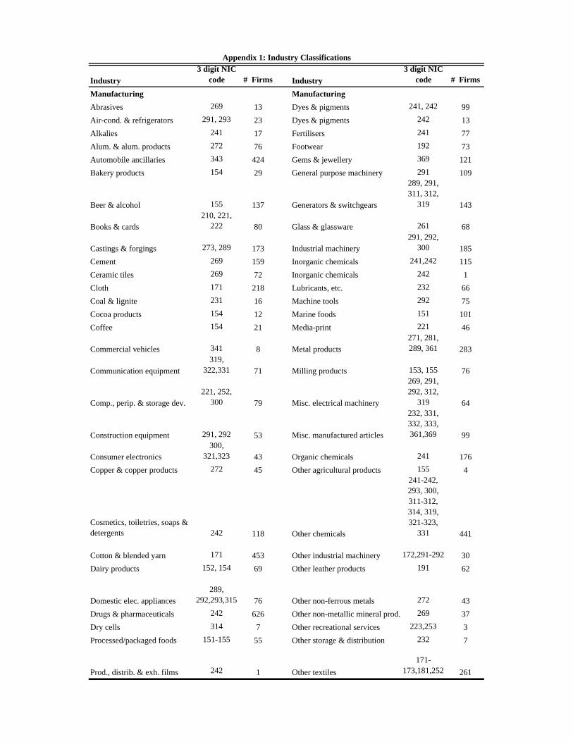
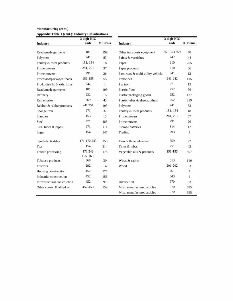
The Indian National Industrial Classification (NIC) (1998) system is used to classify

firms in the Prowess dataset into industries. The data include firms from a wide range of

industries including mining, basic manufacturing, financial and real estate services, and energy

distribution.

The main advantage of firm-level data is that detailed balance sheet and incorporation

information allow us to analyze how incumbent firms are impacted by policy changes such as

liberalization that allow new firm entry. In contrast, industry-level databases usually do not

provide information about sales, assets, and profits by incorporation year and hence firm-age.8

                                                            6 The Prowess database has now been used in several studies including Bertrand et al. (2002), Khanna and Palepu (1999), Fisman and Khanna (2004), Khanna and Palepu (2005), Topalova (2007), Chari and Gupta (2007), and Goldberg et al. (2008, 2009). 7 Unlisted companies are not required to disclose its financials. CMIE asks their permission, but if they refuse, it cannot include these companies in Prowess. 8 Since firms are not required to report employment in their annual reports, we observe employment data for only a more restricted sample of firms. Financial services are the only industry that is mandated by law to disclose

10  

The data allow us to examine whether the ownership composition of firms changed by

the number and size of firms, the fraction of sales, assets and profits by age (incumbent status)

and by industry. We can also examine changes in firm activity and market dynamics in industries

where entry restrictions, both foreign and domestic, were lifted. Appendix 1 provides a

description of variables used in the data analysis.

One concern with the data may be related to new entrants versus improvements in the

data coverage by CMIE. However, for all firms that Prowess decides to cover, regardless of

when the decision is made, financial data from 1989 onwards, wherever available, is added to the

database.

We address the issue of improved coverage in the data versus new entry by making use of

information about incorporation dates. We begin with a sample of firms in 1989 and allow firms

to enter sample only if the new firms enter with data coinciding with their incorporation date.

Therefore, incumbent firms are identified as those firms which had data in 1989 and with

incorporation dates prior to 1989. Following 1991, a firm is identified as a new entrant only if its

data coverage coincides with its incorporation date (also later than 1991). For example a firm

with data coverage beginning in 1992 is deemed to be a new entrant only if its incorporation date

is 1992.

A point about firm-exit is worth noting. The dataset contains a code for firms that exited

the data via mergers and acquisitions. However, the data do not contain a flag for firms shutting

down versus discontinued coverage. Therefore, when we no longer observe data for a firm, we

assume firm-exit. But again, this may also reflect discontinued coverage by Prowess or the

failure of unlisted firms to provide data about their operations. Therefore we construct a balanced

panel of incumbent firms whom we follow over the sample period and an unbalanced panel of

incumbent and new entrant firms where we only allow a new firm to enter the sample if data

availability coincides with the year of incorporation after 1991.

Goldberg et al. (2009) argue that the Prowess dataset is not a manufacturing census, and

therefore may not be ideal for studying firm-entry and exit, given that it includes only larger

firms for which entry and exit are not important margins of adjustment. However, it is pertinent

to note that unlike the Annual Survey of Industries (ASI) which is a survey of manufacturing, the

                                                                                                                                                                  employment information. Since the sample of firms that report employment is small, we do not focus on these numbers.

11  

Prowess data is a panel of firms, rather than a repeated cross-section. Prowess is therefore

particularly well suited to examining how firm- characteristics including entry and exit evolve

over time and may respond to policy changes. (For instance, Goldberg et al. (2009) use the

Prowess dataset to examine how firms adjust their product-mix over time). Firms that no longer

report sales or assets are assumed to have exited. We also classify firms that do not report data

because of mergers and acquisitions as firms that exit the data due to consolidation.

4. Summary Statistics

4.1 The Evolution of Firm Size and Firm Profits

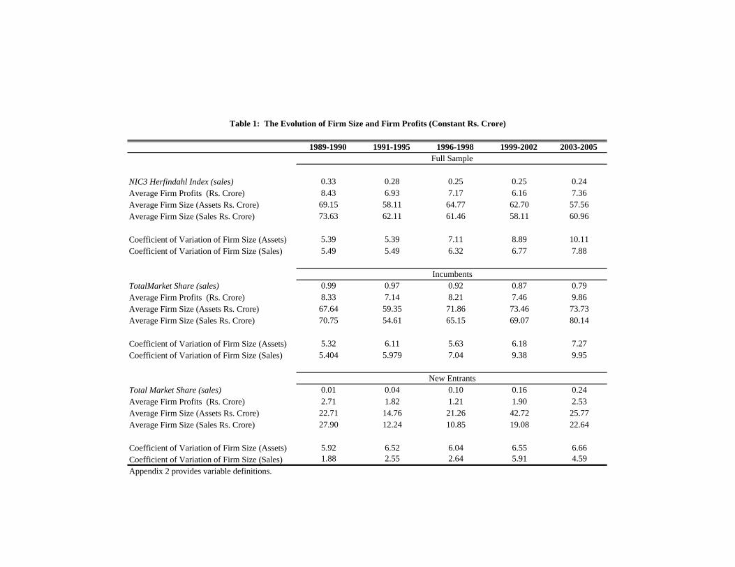
Table 1 includes information on industry concentration (the Herfindahl index9), firm size,

profitability and dispersion measures (coefficient of variation calculated by assets and sales).

Underlying average market share values are calculated for a given firm across the years in a sub-

period and then the Herfindahl index is calculated by industry for a given sub-period. It may be

noted that the Prowess database provides four-and-five-digit industry classifications for most

firms. However, because the liberalization policies were enacted at the three-digit level, industry

concentration accordingly is computed at the three-digit level. We present data for the full

sample first and then by incumbents and new entrants.

For the overall economy, Table 1 shows a reduction in market concentration for the

average firm throughout the sample period. The Herfindahl indices suggest an increased degree

of competition among firms in India. This finding is consistent with the earlier evidence on

increased firm-activity and overall higher dynamism in the economy.

The coefficient of variation (for both sales and assets) also indicates increased dispersion.

Overall, what emerges is a picture of the average manufacturing firm in India growing smaller,

in terms of assets, sales and profits, along with a substantial increase in heterogeneity increased

over the period.

In terms of the differences in incumbent status, for the average incumbent firm,

dispersion has also increased. Overall, the average incumbent firm has grown bigger, more

                                                            9 The Herfindahl index is an indicator of the degree of competition among firms in an industry. It is defined as the square of the market shares of each firm in an industry. The value of the Herfindahl index can range from zero in perfectly competitive industries to one in single-producer monopolies). All data are first expressed in constant rupees crore.

12  

profitable and somewhat more dissimilar.10 While new entrants have also grown significantly in

terms of sales, assets and profits, it is striking to note that the incumbent firms are considerably

bigger than the new entrants. This suggests, consistent with international evidence, that young

firms tend to be small in size and entry takes place from the left hand tail of the size distribution.

For new entrants, dispersion also increases during the sample period.

The total market share variable here refers to the fraction of sales accounted by

incumbent and new entrant firms relative to the total sales in a particular industry. It is

interesting to note that the average market share of incumbent firms in total sales declines from

99% to 79% between 1989 and 2005. Mirroring this decline in average incumbent shares is the

increase in the average market share of new entrants incorporated after 1991 from 1% to 24%

over the same period.11

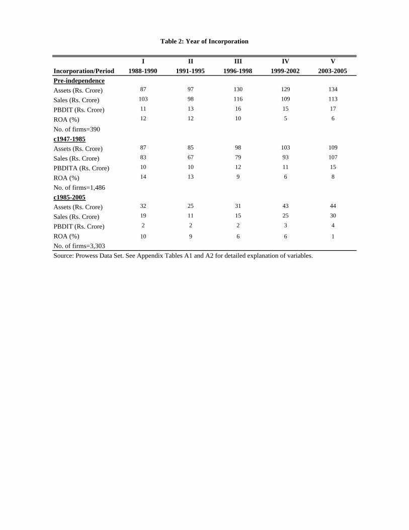
Table 2 presents information by year of incorporation (between pre-1947, 1947-1985,

1985-2005) for number of firms, firm size, assets, sales, employment, profitability, and rate of

return and their evolution in the different periods of study. The oldest firm in the sample

(Howrah Mills Company Ltd.) was incorporated in 1825, and the sample begins with over 390

manufacturing firms that were incorporated before independence. From this group some firms

exit the sample through mergers. Many of these older firms (pre-independence), however,

remain in operation following the reforms.

Tables 3a-c describe how firms evolved before and after in industries that enacted

specific reforms: liberalization of foreign direct investment, trade liberalization and domestic

market deregulation.12

One interesting pattern that emerges from all three panels is that market concentration

seems to have diminished for the liberalizing industries dramatically, following domestic market

regulation, FDI deregulation and trade liberalization (perhaps not very surprising, given the

                                                            10 Note that the average firm profit, sales and assets measures were constructed by taking firm averages by year and industry and then averaging these measures across industries and years with a given time period. For example the average firm asset size of Rs.(crore) 69.15 was constructed by taking the average of average firm assets by industry across industries and over the two year period 1989-1990. 11 Note that the market shares of incumbents and new entrants do not sum to exactly 100% for the following reason. The total market share measure for incumbents was constructed by taking the ratio of total incumbent sales to total industry sales by NIC3 industry and taking an average of this ratio across industries. Similarly, the total market share of new entrants was constructed by taking the ratio of total new entrant sales to total industry sales by NIC3 industry and then averaging this ratio across industries. 12 Variations in the number of industries in Tables10a before and after liberalization reflect entry or exit by different owner categories into industries that were liberalized. The number of industries in the results for the full sample gives the maximum number of liberalized industries.

13  

extent of regulation and lingering restrictions) and consistent with declining incumbent

monopoly power following liberalization. The value of the Herfindahl index declines from 0.43

to 0.27 for industries that liberalized FDI, from 0.48 to 0.27 and 0.26 for industries that

liberalized trade and deregulated domestic entry, respectively.

Table 3a shows measures of measures of market share, firm size, profits and dispersion

averaged across sectors that were for the period before FDI liberalization in the first column and

after FDI liberalization in the second one. The FDI reforms in 1991 reduced barriers to foreign

entry in a subset of industries. According to the Industrial Policy Resolution of 1991, automatic

approval was granted for foreign direct investment of up to 51% in 46 of 96 three-digit industrial

categories (Office of the Economic Advisor, 2001). In the remaining 50 industries, the state

continued to require that foreign investors obtain approval for entry. The top panel of the table

shows the results for the whole sample and the lower ones by incumbent. The sample is

restricted to industries that deregulated foreign investment, to two years before (1989-1990) and

to five years after (1991-1995) the policy was implemented in 1991.

For the average firm, market shares declined significantly following the policy change in

liberalized industries as did average firm profits, sales and assets. Dispersion (both in terms of

assets and sales) increased following the reforms. The average incumbent firm in the liberalized

industries also experienced a decline in market shares, and firm size. However, average

incumbent firm profits in liberalized industries appear to have remained stable. The coefficient of

variation for incumbent firms increased somewhat.

Table 3b presents similar results for trade liberalization. First, it is important to note that

trade liberalization in 1991 was inversely related to industry concentration before 1991. Second,

following trade liberalization, the market share, size and profitability of the average firm in

industries that liberalized trade declined significantly five years following the policy change.

Third, dispersion also increased following trade liberalization. Looking at incumbent firms a

similar pattern obtains except for incumbent firm profits that appear remarkably stable even after

liberalization. Finally, 3c shows similar summary statistics for pre- and post-domestic market

deregulation which shows a similar pattern of declining market shares, size and average firm

profits and increased dispersion.

Strictly speaking, a firm’s market share is equal to firm sales relative to total domestic

industry sales plus imports in that industry. If time-series data were available for imports by 3-

14  

digit NIC code, we would be in a position to adjust our market share calculations for imports. A

caveat to our analysis is therefore that we do not take import figures into account.

Overall, summary statistics suggest that industry concentration, average market shares,

firm size and profits all decline in industries that experienced either de-licensing or FDI and/or

trade liberalization. The coefficient of variation in average firm sales and assets increased

suggesting that there is greater dispersion in firm size within liberalized industries.

4.2 The Evolution of Firm Size-Distributional Statistics

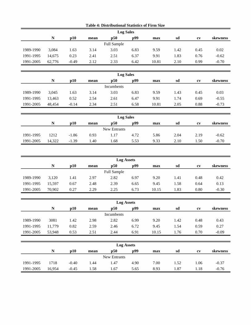
Table 4 presents detailed distributional statistics for firm size in terms of log sales and log

assets before and after liberalization. For both assets and sales, the mean and median numbers

suggest that firm size declined over the sample period and the pattern holds for incumbent firms

as well. New entrants on the other hand experience an increase in firm size, perhaps not

surprisingly.

Examining the tails of the size distribution reveals two interesting patterns. First, we see

that the smallest firms in the left hand tail of the size distribution have become smaller over time.

The firms in the tenth percentile have grown considerably smaller over the post liberalization

period. The data suggests also that firm entry has taken place in the form of small firms

especially since the new entrants are much smaller than the incumbent firms in the lowest

percentiles of size for both assets and sales.

Second, the largest firms have grown bigger. For all three samples, the full sample,

incumbents and new entrants the largest firms in the 99th percentile have grown larger over time.

It is particularly interesting to note the increase in the size of the largest new entrants.

These two patterns from the distributional data (small firms getting smaller and big firms

bigger) are consistent with an increase in the standard deviation in the size distribution. Also

given the increase in the standard deviation of firm size and the fall in the average firm size, it is

perhaps not surprising that dispersion measured by the coefficient of variation in firm size rises.

Note that these preliminary findings from the size distribution data are not entirely

consistent with the predictions from Melitz (2003) and Melitz and Ottaviano (2008) which

expect that average firm size should rise. While the largest firms increase in size, there also

appears to be considerable entry from the left hand tail of the distribution and the average size

for the smallest incumbent firms also appears to get smaller. In addition, average firm size and

15  

average firm profits fall not rise as predicted in these models. The findings are however

consistent with Blanchard and Giavazzi (2003) and Alesina et al. (2005) where, on average,

incumbent firms are predicted to lose monopoly power following deregulation. The marginal

entry of small firms is consistent with an increase in competition following entry deregulation.

The final column of Table 4 shows that the size distribution becomes negatively skewed

over time. The pattern is more clearly seen in Charts 1-6. The size distribution flattens and shifts

in the direction of negative skewness following liberalization with the magnitude of skewness

increasing over time. The size distribution in the early years following liberalization (1991-1995)

is more skewed in comparison to the pre-liberalization period (1989-1990), and the size

distribution in the later years following liberalization (2003-2005) is more skewed in comparison

to the early years. The shift in the pattern of skewness holds for both log assets and log sales as

well as for the incumbent firms.

5. Empirical Methodology and Results

We now turn to the formal estimations of the impact of deregulation on firm size and

profitability. We begin by considering a balanced panel of incumbent firms that existed before

liberalization. To examine the impact of deregulation and entry, a restricted sample panel of

incumbent firms is better suited to analyzing pre- and post- effects on these firms. By restricting

the sample to incumbent firms, we are able to parse out compositional effects that occur with

entry. We first look at the impact of deregulation on incumbent firms without firm-fixed effects

to examine more cleanly what happens to incumbent firms. We then introduce compositional

controls in the form of firm-fixed effects to control for unobserved heterogeneity at the firm-

level. However, a specification with firm-fixed effects cannot use this to examine distributional

effects which occur with entry. To do so, we examine an unbalanced panel that allows for

compositional effects to occur with entry.

We begin with the following benchmark regression specification, for firm i in sector j and

year t:

Yijt = ai + Yeart + d Libjt + + eijt (1)

where Yjjt : different outcome variables, we control for firm fixed effects and a year trend.

Standard errors are robust and clustered at the 3-digit industry level.

16  

Since the sample period in this paper coincides with a period of rapid growth in the

Indian economy, incorporate a linear year trend in our estimations to more precisely isolate the

impact of the liberalization policy measures. We report estimates with and without the year trend

to highlight the impact on the coefficient estimates and their interpretation.

5.1 Balanced Panel

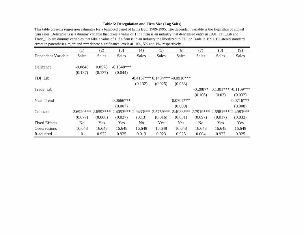
Table 5 presents regression estimates for a balanced panel of firms from 1989-1995. The

dependent variable is the logarithm of annual firm sales. Delicense is a dummy variable that

takes a value of 1 if a firm is an industry that delicensed entry in 1991. FDI_Lib and Trade_Lib

are dummy variables that take a value of 1 if a firm is in an industry the liberalized to FDI or

Trade in 1991. Standard errors are clustered at the NIC3-digit level.

Columns 1, 4 and 7 show the impact of deregulation on log sales for incumbent firms

without fixed effects. While the impact of delicensing appears to have an insignificant effect on

firm sales, both trade and FDI liberalization leading to a decline in average incumbent firm sales.

Controlling for firm-fixed effects in Columns 2, 5 and 8 shows that while the impact of

delicensing continues to be insignificant, average incumbent firm size increases significantly

with trade and FDI liberalization. Note that the sign on the coefficient for both the trade and FDI

liberalization dummies flips when we introduce firm-fixed effects suggesting that the average

incumbent firm grew over this time period.

As we argue earlier, to account for the rapid growth in the economy over this time period,

we incorporate a year trend variable into the specifications in columns 3, 6 and 9. The coefficient

on the delicensing dummy is now negative and significant. Interestingly, the coefficients on the

trade and FDI dummies are negative and significant once again while the coefficient on the year

trend is positive and significant.

The results from the specification suggest that the impact of deregulation on firm size in

the context of a growing economy can be decomposed into two effects: a competitive effect

through firm entry and a growth effect. Competition through entry appears to reduce average

firm size while the growing economy lifts all boats increasing average firm size. Incorporating

the year trend variable is important therefore not only because it allows us to isolate the impact

of deregulation on firm size but also because it suggests that a dynamic model is better suited to

17  

examining the effects of deregulation on competition against the backdrop of a growing

economy.

Table 6 repeats the analysis for log assets and a similar pattern obtains. It is important to

note that the negative and significant coefficient on the deregulation dummies (delicense, trade

and FDI) are consistent with two alternative interpretations. The negative coefficient on the

liberalization dummies with positive year trend coefficient could be interpreted as (i) average

firm size goes down in liberalized industries but also (ii) controlling for the overall growth of the

economy, liberalized industries are growing slower.

5.2 Unbalanced Panel As stated earlier, with unbalanced panels we allow for compositional effects to occur with

entry. We turn to quantile regressions are important for looking at distribution effects on firm

size. Quantile (including median) regression models, also known as least-absolute value (LAV)

models or minimum absolute deviation (MAD) models. In the median regression estimates

version of the quantile regression model, the median of the dependent variable is analyzed

conditional on the values of the independent variable. This is similar to least-squares regression,

which estimates the mean of the dependent variable. Put differently, quantile regressions find the

regression plane that minimizes the sum of the absolute residuals rather than the sum of the

squared residuals.

Since we are interested in characterizing the entire distribution of firm size before and

after deregulation, we specify a regression specification that estimates the regression plane for

quantiles ranging from the 5th percentile to the 95th percentile of the distribution of the outcome

variable of interest (size, profits) at intervals of 5%. Standard errors are bootstrapped.

As described by Koenker and Bassett (1978), the estimation is done by minimizing the

following specification:

∑ | |: ∑ 1 | |:                                     (2)                             

 

where y is the dependent variable, x is the k by 1 vector of explanatory variables, b is the

coefficient vector and 1 is the quantile to be estimated. The coefficient vector b will differ

depending on the particular quantile being estimated.

18  

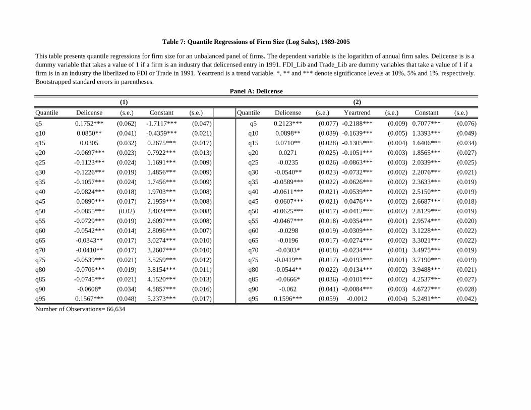
Table 7 estimates the quantile regression specification with log sales as the dependent

variable and with the deregulation dummies (delicense, trade and FDI) and the independent

variables. A second specification includes the year trend variable. The coefficients on the

deregulation dummies display considerable non-linearity and highlight the heterogeneous effects

of deregulation on firms of different sizes.

Table 7 shows that the impact of delicensing on log sales for firms across quantiles of

differing firm sizes is non-linear. There is an increase in the average firm size for firms in the 5th

through the 15th percentile consistent with entry by small firms from the left hand tail. There is

however, a significant decline for all quantiles from the 20th to the 90th percentile. Finally, the

coefficient for the 95th percentile is positive and significant consistent with large incumbents

growing bigger and perhaps being exporters as in the Melitz and Ottaviano (2008) model.

Adding a year trend shifts quantile regression coefficients curve up. These results should

be interpreted with caution as we do not include fixed effects. Also, the significance of

coefficient estimates varies once the year trend is included. Here, the negative coefficient on the

year trend indicates that the average firm size declines as the market size grows. The non-linear

effects on firm size are also seen when the regressions include the trade and FDI dummies. The

pattern of the firms in the 95th percentile getting bigger is only seen with FDI liberalization

when the year trend is included but not with trade liberalization reducing tariffs on imports.

Chart 3 depicts these findings graphically to highlight the non-linear impact of

delicensing, FDI and trade liberalization on firm size across quantiles. It also serves to highlight

the varying magnitude of the coefficient estimates across quantiles. The three panels show the

impact of adding a year trend shifts the magnitude of the coefficient estimates on the

deregulation measures on firm size.

5.3 Deregulation, Market Concentration and Profitability

Table 8 presents regression estimates for an unbalanced panel of firms from 1989-1995.

The dependent variable is the Herfindahl index of firm sales. The independent variables are the

deregulation dummies. Standard errors are clustered at the 3-digit NIC industry level. Consistent

with an increase in competitiveness and with the summary statistics in Table 3, the Herfindahl

index declines significantly in industries that were deregulated. The pattern of declining

Herfindahl indices is also seen when we estimate a specification with a balanced panel of

19  

incumbent firms although with a slightly smaller magnitude of coefficient estimates suggesting a

decline in the monopoly power of incumbent firms with deregulation consistent with the

predictions from Blanchard and Giavazzi (2003). The Herfindahl index also shows a significant

decline if we restrict the sample period to the immediate aftermath of the deregulation in 1991-

1995. The magnitudes are smaller but significant with the exception of the coefficient on the

delicensing dummy.

Table 9 estimates the quantile regression specification with the return on assets as the

dependent variable and with the deregulation dummies (delicense, trade and FDI) and the

independent variables. A second specification includes the year trend variable. The coefficients

on the deregulation dummies display considerable non-linearity and highlight the heterogeneous

effects of deregulation on firms of differing profitability. A note of caution is that the return on

asset series is very noisy with extreme outliers both negative and positive. Therefore, it is not

clear the weight we can place on the patterns observed. Once again, the specifications do not

include firm fixed effects.

The coefficient estimates indicate that while the return on assets declined significantly in

industries that were delicensed consistent with greater competition via entry, the return on assets

actually increased significantly for the specifications that include FDI and trade liberalization.

Chart 4 displays these results graphically.

6. Conclusion

India has engaged in a massive deregulation effort since 1991. The end of the license Raj

and implementation of pro-market reforms have far-reaching implications for competitive

environment in the Indian economy. Significant sectors of the economy were opened up for

private participation through de-licensing and allowing entry in industries previously reserved

exclusively for the state-owned sector. Trade liberalization allowing for more import competition

by reducing tariff and other trade barriers has also been considerable. At the same time, many

sectors of the economy have been opened to foreign entry via direct investment.

Nearly twenty years after the reforms began we ask whether liberalization has led to more

competition. We argue that an increase in competition may be measured in several ways.

Deregulating entry may imply an increase in dispersion in firm size distributions, a reduction in

concentration ratios or a decline in average firm size and profits. To examine the competitive

20  

effects of deregulating entry, we use firm-level data from CMIE’s Prowess database to examine

the changes in firm size and profitability distributions.

The evidence suggests several interesting patterns. Average firm size declines

significantly in industries that deregulated entry. Small firms enter the market from the left hand

tail of the size distribution while the incumbent firms get significantly bigger following

deregulation. Quantile regressions to examine the distributional impact of deregulation show that

the shift in the distribution of firm size is non-linear with average firm size increasing till around

the 15th percentile, and then getting significantly smaller till the 90th percentile while the largest

percentile (95%) gets significantly bigger over the same time period.

Consistent with a decline in monopoly power, the Herfindahl index of firm sales also

shows a significant decline. While summary statistics suggest a decline in average firm profits,

quantile regressions once again show significant non-linearity and a heterogeneous impact of

deregulation on profitability. The dispersion of firm size (sales and assets) also rises following

deregulation consistent with Melitz and Ottaviano (2008), Campbell and Hopenhayen (2005),

and Asplund and Nocke (2003).

On balance, the evidence suggests that examining the distributional changes in firm size

and profitability reveal the more nuanced effects of deregulation. The marginal entry of small

firms and the decline in the average size of firms in the middle percentiles appears consistent

with the hypothesis that deregulation leads to entry, a larger number of firms in the long run, and

the reduction in the monopoly power of firms. However, the increase in the size of the largest

firms suggests that it is important to take into account the possible non-linear effects of

deregulation on competition.

21  

References Alesina, Alberto, Silvia Ardagna, Giuseppe Nicoletti and Fabio Schiantarelli, 2005. “Regulation

and Investment, ”Journal of the European Economic Association, 3(4):791–825.

Alfaro, Laura and Anusha Chari, 2010a. "India Transformed? Insights from the Firm Level 1988-

2005" Brookings India Policy Forum Journal, 2010, Vol. 6, pp. 155-228.

Asplund , M. and V. Nocke, 2003. “Firm Turnover in Imperfectly Competitive Markets,” PIER

Working Paper Archive 03-010, Penn Institute for Economic Research, Department of

Economics, University of Pennsylvania.

Berry, Steven and Peter Reiss (2007), “Empirical Models of Entry and Market Structure,"

Chapter 29 in Handbook of Industrial Organization, vol. 3, Mark Armstrong and

Robert Porter, eds. North-Holland Press.

Bertrand, M, P. Mehta and S. Mullainathan, 2002. “Ferreting Out Tunneling: An Application to

Indian Business groups,” Quarterly Journal of Economics, 121-148.

Blanchard, O. J. and F. Giavazzi, 2003. “Macroeconomic Effects of Regulation and Deregulation

in Goods and Labor Market,” Quarterly Journal of Economics 118, 879–908.

Campbell, J. R. and H. A. Hopenhayn, 2005. “Market Size Matters,” Journal of Industrial

Economics, Blackwell Publishing, vol. 53(1), 1-25, 03.

Chari, A. and N. Gupta, 2008. “Incumbents and Protectionism: The Political Economy of

Foreign Entry Liberalization.” Journal of Financial Economics 88, 33-656.

Fisman, R. and T. Khanna, 2004. “Facilitating Development: The Role of Business Groups,”

World Development 32, 609-28.

Goldberg, P., A. Khandelwal, N. Pavcnik and P. Topalova, 2009. “Trade Liberalization and New

Imported Inputs,” mimeo.

Goldberg, P., A. Khandelwal, N. Pavcnik and P. Topalova, 2008. “Imported Intermediate Inputs

and Domestic Product Growth: Evidence from India,” NBER Working Paper 14416.

Office of the Economic Advisor, 2001. Handbook of industrial policy and statistics. Government

of India, New Delhi.

Khanna, T. and K. Palepu, 1999. “Policy Shocks, Market Intermediaries and Corporate Strategy:

the Evolution of Business Groups in Chile and India,” Journal of Economics &

Management Strategy 8, 271-310.

22  

Khanna, T. and K. Palepu, 2005. “The Evolution of Concentrated Ownership in India: Broad

Patterns and a History of the Indian Software Industry,” in Randall Morck, eds., A

History of Corporate Governance around the World: Family Business Groups to

Professional Managers, University of Chicago Press.

Koenker, Roger W & Bassett, Gilbert, Jr, 1978. "Regression Quantiles," Econometrica, 46(1),

33-50.

Melitz, M. J., 2003. “The Impact of Trade on Intra-Industry Reallocations and Aggregate

Industry Productivity,” Econometrica 71, 1695-1725.

Melitz, M. and G. Ottaviano, 2008. “Market Size, Trade, and Productivity,” Review of Economic

Studies 75, 295-316.

Syverson, C., 2004. “Market Structure and Productivity: A Concrete Example,” Journal of

Political Economy, University of Chicago Press, vol. 112(6), 1181-1222.

Topalova, P., 2007. “Trade Liberalization and Firm Productivity: The Case of India,” IMF

Working Paper, WP/04/28.

Industry3 digit NIC

code # Firms Industry3 digit NIC

code # Firms

Manufacturing Manufacturing Abrasives 269 13 Dyes & pigments 241, 242 99Air-cond. & refrigerators 291, 293 23 Dyes & pigments 242 13Alkalies 241 17 Fertilisers 241 77Alum. & alum. products 272 76 Footwear 192 73Automobile ancillaries 343 424 Gems & jewellery 369 121Bakery products 154 29 General purpose machinery 291 109

Beer & alcohol 155 137 Generators & switchgears

289, 291, 311, 312,

319 143

Books & cards210, 221,

222 80 Glass & glassware 261 68

Castings & forgings 273, 289 173 Industrial machinery291, 292,

300 185Cement 269 159 Inorganic chemicals 241,242 115Ceramic tiles 269 72 Inorganic chemicals 242 1Cloth 171 218 Lubricants, etc. 232 66Coal & lignite 231 16 Machine tools 292 75Cocoa products 154 12 Marine foods 151 101Coffee 154 21 Media-print 221 46

Commercial vehicles 341 8 Metal products271, 281, 289, 361 283

Communication equipment319,

322,331 71 Milling products 153, 155 76

Comp., perip. & storage dev.221, 252,

300 79 Misc. electrical machinery

269, 291, 292, 312,

319 64

Construction equipment 291, 292 53 Misc. manufactured articles

232, 331, 332, 333, 361,369 99

Consumer electronics300,

321,323 43 Organic chemicals 241 176Copper & copper products 272 45 Other agricultural products 155 4

Cosmetics, toiletries, soaps & detergents 242 118 Other chemicals

241-242, 293, 300, 311-312, 314, 319, 321-323,

331 441

Cotton & blended yarn 171 453 Other industrial machinery 172,291-292 30Dairy products 152, 154 69 Other leather products 191 62

Domestic elec. appliances289,

292,293,315 76 Other non-ferrous metals 272 43Drugs & pharmaceuticals 242 626 Other non-metallic mineral prod. 269 37Dry cells 314 7 Other recreational services 223,253 3Processed/packaged foods 151-155 55 Other storage & distribution 232 7

Prod., distrib. & exh. films 242 1 Other textiles171-

173,181,252 261

Appendix 1: Industry Classifications

Manufacturing (cont.)Appendix Table 1 (cont.): Industry Classifications

Industry3 digit NIC

code # Firms Industry3 digit NIC

code # Firms

Readymade garments 181 199 Other transports equipment 351-353,359 48Polymers 241 83 Paints & varnishes 242 44Poultry & meat products 151, 154 18 Paper 210 205Prime movers 281, 291 37 Paper products 210 66Prime movers 291 26 Pass. cars & multi utility vehicles 341 12Processed/packaged foods 151-155 55 Pesticides 241-242 115Prod., distrib. & exh. films 242 1 Pig iron 271 13Readymade garments 181 199 Plastic films 252 56Refinery 232 15 Plastic packaging goods 252 137Refractories 269 43 Plastic tubes & sheets, others 252 219Rubber & rubber products 241,251 105 Polymers 241 83Sponge iron 271 32 Poultry & meat products 151, 154 18Starches 153 13 Prime movers 281, 291 37Steel 271 488 Prime movers 291 26Steel tubes & pipes 271 111 Storage batteries 314 12Sugar 154 147 Trading 293 1

Synthetic textiles 171-172,243 158 Two & three wheelers 359 22Tea 154 214 Tyres & tubes 251 42Textile processing 171,243 176 Vegetable oils & products 151-153 307

Tobacco products155, 160,

369 30 Wires & cables 313 110Tractors 292 14 Wood 201-202 53Housing construction 452 177 261 1Industrial construction 452 156 343 1Infrastructural construction 452 91 Diversified 970 63Other constr. & allied act. 452-453 159 Misc. manufactured articles 970 695

Misc. manufactured articles 970 695

Variables Definition

Sales Sales generated by a firm from its main business activity measured by charges to customers for goodssupplied and services rendered. Excludes income from activities not related to main business, such asdividends, interest, and rents in the case of industrial firms, as well as non-recurring income.

Assets Gross fixed assets of a firm, which includes movable and immovable assets as well as assets which are in theprocess of being installed.

Firm Size (Assets & Sales) Average firm assets and sales in an industry. For the full sample, the industry-level averages are averagedacross industries.

Market Share Ratio of Sales to Industry Sales for a firm. Also, ratio of Assets to Industry Assets for a firm.

Herfindahl Index Sum of the squares of the Market Share of all firms in an industry in each 3-digit industrial category.

Incumbent Share The ratio of total sales, assets, profits produced by incumbent firms (incorporated before 1990) in an industryto Industry Sales , Industry Assets, Industry Profits in that industry.

New Entrant Share The ratio of total sales, assets, profits produced by new entrant firms (incorporated after 1991) in an industryto Industry Sales , Industry Assets, Industry Profits in that industry.

Industry Sales Sum of Sales across all firms in an industry.

Industry Assets Sum of Assets across all firms in an industry.

PBITDA Excess of income over all expenditures except tax, depreciation, interest payments, and rents in a firm.

Return on Assets Ratio of PBITDA to Assets in a firm, averaged across firms in that industry.

Sales Growth (Industry Sales -Lagged Industry Sales )/Lagged Industry Sales in that industry.

Coefficient of Variation Ratio of standard deviation to mean of assets, sales, return on assets at the industry level

Tade liberalization measure Percentage decrease in tariffs at the three-digit industry level between 1986-1990 and 1991-1995.

NIC Code Three-digit industry code includes manufacturing, financial, and service sectors.

Appendix 2 - Description of Variables

1989-1990 1991-1995 1996-1998 1999-2002 2003-2005

NIC3 Herfindahl Index (sales) 0.33 0.28 0.25 0.25 0.24Average Firm Profits (Rs. Crore) 8.43 6.93 7.17 6.16 7.36Average Firm Size (Assets Rs. Crore) 69.15 58.11 64.77 62.70 57.56Average Firm Size (Sales Rs. Crore) 73.63 62.11 61.46 58.11 60.96 Coefficient of Variation of Firm Size (Assets) 5.39 5.39 7.11 8.89 10.11Coefficient of Variation of Firm Size (Sales) 5.49 5.49 6.32 6.77 7.88

TotalMarket Share (sales) 0.99 0.97 0.92 0.87 0.79Average Firm Profits (Rs. Crore) 8.33 7.14 8.21 7.46 9.86Average Firm Size (Assets Rs. Crore) 67.64 59.35 71.86 73.46 73.73Average Firm Size (Sales Rs. Crore) 70.75 54.61 65.15 69.07 80.14 Coefficient of Variation of Firm Size (Assets) 5.32 6.11 5.63 6.18 7.27Coefficient of Variation of Firm Size (Sales) 5.404 5.979 7.04 9.38 9.95

Total Market Share (sales) 0.01 0.04 0.10 0.16 0.24Average Firm Profits (Rs. Crore) 2.71 1.82 1.21 1.90 2.53Average Firm Size (Assets Rs. Crore) 22.71 14.76 21.26 42.72 25.77Average Firm Size (Sales Rs. Crore) 27.90 12.24 10.85 19.08 22.64 Coefficient of Variation of Firm Size (Assets) 5.92 6.52 6.04 6.55 6.66Coefficient of Variation of Firm Size (Sales) 1.88 2.55 2.64 5.91 4.59Appendix 2 provides variable definitions.

Table 1: The Evolution of Firm Size and Firm Profits (Constant Rs. Crore)

Full Sample

Incumbents

New Entrants

I II III IV VIncorporation/Period 1988-1990 1991-1995 1996-1998 1999-2002 2003-2005Pre-independenceAssets (Rs. Crore) 87 97 130 129 134

Sales (Rs. Crore) 103 98 116 109 113

PBDIT (Rs. Crore) 11 13 16 15 17

ROA (%) 12 12 10 5 6

No. of firms=390c1947-1985Assets (Rs. Crore) 87 85 98 103 109

Sales (Rs. Crore) 83 67 79 93 107

PBDITA (Rs. Crore) 10 10 12 11 15

ROA (%) 14 13 9 6 8

No. of firms=1,486c1985-2005Assets (Rs. Crore) 32 25 31 43 44

Sales (Rs. Crore) 19 11 15 25 30

PBDIT (Rs. Crore) 2 2 2 3 4

ROA (%) 10 9 6 6 1No. of firms=3,303Source: Prowess Data Set. See Appendix Tables A1 and A2 for detailed explanation of variables.

Table 2: Year of Incorporation

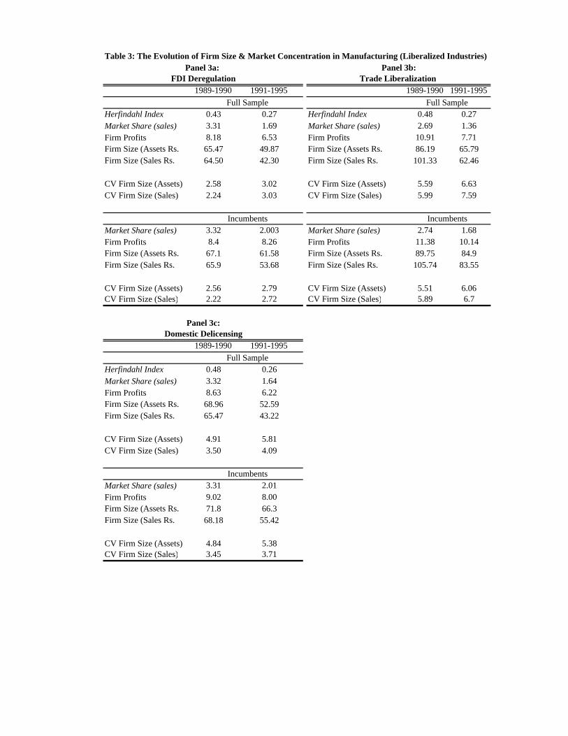
Table 3: The Evolution of Firm Size & Market Concentration in Manufacturing (Liberalized Industries)

1989-1990 1991-1995 1989-1990 1991-1995

Herfindahl Index 0.43 0.27 Herfindahl Index 0.48 0.27Market Share (sales) 3.31 1.69 Market Share (sales) 2.69 1.36Firm Profits 8.18 6.53 Firm Profits 10.91 7.71Firm Size (Assets Rs. 65.47 49.87 Firm Size (Assets Rs. 86.19 65.79Firm Size (Sales Rs. 64.50 42.30 Firm Size (Sales Rs. 101.33 62.46 CV Firm Size (Assets) 2.58 3.02 CV Firm Size (Assets) 5.59 6.63CV Firm Size (Sales) 2.24 3.03 CV Firm Size (Sales) 5.99 7.59

Market Share (sales) 3.32 2.003 Market Share (sales) 2.74 1.68Firm Profits 8.4 8.26 Firm Profits 11.38 10.14Firm Size (Assets Rs. 67.1 61.58 Firm Size (Assets Rs. 89.75 84.9Firm Size (Sales Rs. 65.9 53.68 Firm Size (Sales Rs. 105.74 83.55 CV Firm Size (Assets) 2.56 2.79 CV Firm Size (Assets) 5.51 6.06CV Firm Size (Sales) 2.22 2.72 CV Firm Size (Sales) 5.89 6.7

1989-1990 1991-1995

Herfindahl Index 0.48 0.26Market Share (sales) 3.32 1.64Firm Profits 8.63 6.22Firm Size (Assets Rs. 68.96 52.59Firm Size (Sales Rs. 65.47 43.22 CV Firm Size (Assets) 4.91 5.81CV Firm Size (Sales) 3.50 4.09

Market Share (sales) 3.31 2.01Firm Profits 9.02 8.00Firm Size (Assets Rs. 71.8 66.3Firm Size (Sales Rs. 68.18 55.42 CV Firm Size (Assets) 4.84 5.38CV Firm Size (Sales) 3.45 3.71

Panel 3b:

Full Sample

Incumbents

Panel 3a:

Panel 3c:

Full Sample

FDI Deregulation Trade Liberalization

Full Sample

Incumbents

Incumbents

Domestic Delicensing

N p10 mean p50 p99 max sd cv skewnessFull Sample

1989-1990 3,084 1.63 3.14 3.03 6.83 9.59 1.42 0.45 0.021991-1995 14,675 0.23 2.41 2.51 6.37 9.91 1.83 0.76 -0.621991-2005 62,776 -0.49 2.12 2.33 6.42 10.81 2.10 0.99 -0.70

N p10 mean p50 p99 max sd cv skewnessIncumbents

1989-1990 3,045 1.63 3.14 3.03 6.83 9.59 1.43 0.45 0.031991-1995 13,463 0.52 2.54 2.61 6.47 9.91 1.74 0.69 -0.551991-2005 48,454 -0.14 2.34 2.51 6.58 10.81 2.05 0.88 -0.73

N p10 mean p50 p99 max sd cv skewnessNew Entrants

1991-1995 1212 -1.86 0.93 1.17 4.72 5.86 2.04 2.19 -0.621991-2005 14,322 -1.39 1.40 1.68 5.53 9.33 2.10 1.50 -0.70

N p10 mean p50 p99 max sd cv skewnessFull Sample

Table 4: Distributional Statistics of Firm Size Log Sales

Log Sales

Log Sales

Log Assets

p1989-1990 3,120 1.41 2.97 2.82 6.97 9.20 1.41 0.48 0.421991-1995 15,597 0.67 2.48 2.39 6.65 9.45 1.58 0.64 0.131991-2005 70,902 0.27 2.29 2.25 6.73 10.15 1.83 0.80 -0.30

N p10 mean p50 p99 max sd cv skewnessIncumbents

1989-1990 3081 1.42 2.98 2.82 6.99 9.20 1.42 0.48 0.431991-1995 11,779 0.82 2.59 2.46 6.72 9.45 1.54 0.59 0.271991-2005 53,948 0.53 2.51 2.44 6.91 10.15 1.76 0.70 -0.09

N p10 mean p50 p99 max sd cv skewnessNew Entrants

1991-1995 1718 -0.40 1.44 1.47 4.90 7.00 1.52 1.06 -0.371991-2005 16,954 -0.45 1.58 1.67 5.65 8.93 1.87 1.18 -0.76

Log Assets

Log Assets

(1) (2) (3) (4) (5) (6) (7) (8) (9)Dependent Variable Sales Sales Sales Sales Sales Sales Sales Sales Sales

Delicence -0.0848 0.0578 -0.1640***(0.137) (0.137) (0.044)

FDI_Lib -0.4157*** 0.1484*** -0.0910***(0.132) (0.025) (0.033)

Trade_Lib -0.2087* 0.1301*** -0.1109***(0.106) (0.03) (0.032)

Year Trend 0.0666*** 0.0707*** 0.0716***(0.007) (0.009) (0.008)

Constant 2.6920*** 2.6593*** 2.4053*** 2.9433*** 2.5759*** 2.4083*** 2.7919*** 2.5981*** 2.4083***(0.077) (0.008) (0.027) (0.13) (0.016) (0.031) (0.097) (0.017) (0.032)

Fixed Effects No Yes Yes No Yes Yes No Yes YesObservations 16,648 16,648 16,648 16,648 16,648 16,648 16,648 16,648 16,648R-squared 0 0.922 0.925 0.013 0.923 0.925 0.004 0.922 0.925

This table presents regression estimates for a balanced panel of firms from 1989-1995. The dependent variable is the logarithm of annual firm sales. Delicense is is a dummy variable that takes a value of 1 if a firm is an industry that delicensed entry in 1991. FDI_Lib and Trade_Lib are dummy variables that take a value of 1 if a firm is in an industry the liberlized to FDI or Trade in 1991. Clustered standard errors in parentheses. *, ** and *** denote significance levels at 10%, 5% and 1%, respectively.

Table 5: Deregulation and Firm Size (Log Sales)

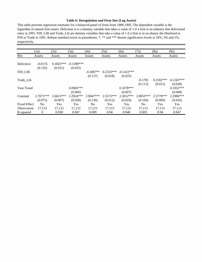
(1a) (2a) (3a) (4a) (5a) (6a) (7a) (8a) (9a)Rhs Assets Assets Assets Assets Assets Assets Assets Assets Assets

Delicence -0.0174 0.1825*** -0.1398***(0.135) (0.031) (0.033)

FDI_LIB -0.3087** 0.2233*** -0.1422***(0.137) (0.018) (0.025)

Trade_Lib -0.1781 0.2182*** -0.1367***(0.113) (0.015) (0.028)

Year Trend 0.0965*** 0.1078*** 0.1052***(0.006) (0.007) (0.008)

Constant 2.7071*** 2.6613*** 2.2924*** 2.9047*** 2.5573*** 2.3012*** 2.8053*** 2.5779*** 2.2986***(0.075) (0.007) (0.028) (0.136) (0.012) (0.024) (0.104) (0.009) (0.026)

Fixed Effect No Yes Yes No Yes Yes No Yes YesObservation 17,115 17,115 17,115 17,115 17,115 17,115 17,115 17,115 17,115R-squared 0 0.938 0.947 0.009 0.94 0.948 0.003 0.94 0.947

This table presents regression estimates for a balanced panel of firms from 1989-1995. The dependent variable is the logarithm of annual firm assets. Delicense is is a dummy variable that takes a value of 1 if a firm is an industry that delicensed entry in 1991. FDI_LIB and Trade_Lib are dummy variables that take a value of 1 if a firm is in an idustry the liberlized to FDI or Trade in 1991. Robust standard errors in parentheses. *, ** and *** denote significance levels at 10%, 5% and 1%, respectively.

Table 6: Deregulation and Firm Size (Log Assets)

Quantile Delicense (s.e.) Constant (s.e.) Quantile Delicense (s.e.) Yeartrend (s.e.) Constant (s.e.)q5 0.1752*** (0.062) -1.7117*** (0.047) q5 0.2123*** (0.077) -0.2188*** (0.009) 0.7077*** (0.076) q10 0.0850** (0.041) -0.4359*** (0.021) q10 0.0898** (0.039) -0.1639*** (0.005) 1.3393*** (0.049) q15 0.0305 (0.032) 0.2675*** (0.017) q15 0.0710** (0.028) -0.1305*** (0.004) 1.6406*** (0.034) q20 -0.0697*** (0.023) 0.7922*** (0.013) q20 0.0271 (0.025) -0.1051*** (0.003) 1.8565*** (0.027) q25 -0.1123*** (0.024) 1.1691*** (0.009) q25 -0.0235 (0.026) -0.0863*** (0.003) 2.0339*** (0.025) q30 -0.1226*** (0.019) 1.4856*** (0.009) q30 -0.0540** (0.023) -0.0732*** (0.002) 2.2076*** (0.021) q35 -0.1057*** (0.024) 1.7456*** (0.009) q35 -0.0589*** (0.022) -0.0626*** (0.002) 2.3633*** (0.019) q40 -0.0824*** (0.018) 1.9703*** (0.008) q40 -0.0611*** (0.021) -0.0539*** (0.002) 2.5150*** (0.019) q45 -0.0890*** (0.017) 2.1959*** (0.008) q45 -0.0607*** (0.021) -0.0476*** (0.002) 2.6687*** (0.018) q50 -0.0855*** (0.02) 2.4024*** (0.008) q50 -0.0625*** (0.017) -0.0412*** (0.002) 2.8129*** (0.019) q55 -0.0729*** (0.019) 2.6097*** (0.008) q55 -0.0467*** (0.018) -0.0354*** (0.001) 2.9574*** (0.020) q60 -0.0542*** (0.014) 2.8096*** (0.007) q60 -0.0298 (0.019) -0.0309*** (0.002) 3.1228*** (0.022) q65 -0.0343** (0.017) 3.0274*** (0.010) q65 -0.0196 (0.017) -0.0274*** (0.002) 3.3021*** (0.022) q70 -0.0410** (0.017) 3.2607*** (0.010) q70 -0.0303* (0.018) -0.0234*** (0.001) 3.4975*** (0.019) q75 -0.0539*** (0.021) 3.5259*** (0.012) q75 -0.0419** (0.017) -0.0193*** (0.001) 3.7190*** (0.019) q80 -0.0706*** (0.019) 3.8154*** (0.011) q80 -0.0544** (0.022) -0.0134*** (0.002) 3.9488*** (0.021) q85 -0.0745*** (0.021) 4.1520*** (0.013) q85 -0.0666* (0.036) -0.0101*** (0.002) 4.2537*** (0.027) q90 -0.0608* (0.034) 4.5857*** (0.016) q90 -0.062 (0.041) -0.0084*** (0.003) 4.6727*** (0.028) q95 0.1567*** (0.048) 5.2373*** (0.017) q95 0.1596*** (0.059) -0.0012 (0.004) 5.2491*** (0.042) Number of Observations= 66,634

This table presents quantile regressions for firm size for an unbalanced panel of firms. The dependent variable is the logarithm of annual firm sales. Delicense is is a dummy variable that takes a value of 1 if a firm is an industry that delicensed entry in 1991. FDI_Lib and Trade_Lib are dummy variables that take a value of 1 if a firm is in an industry the liberlized to FDI or Trade in 1991. Yeartrend is a trend variable. *, ** and *** denote significance levels at 10%, 5% and 1%, respectively. Bootstrapped standard errors in parentheses.

Table 7: Quantile Regressions of Firm Size (Log Sales), 1989-2005

Panel A: Delicense(1) (2)

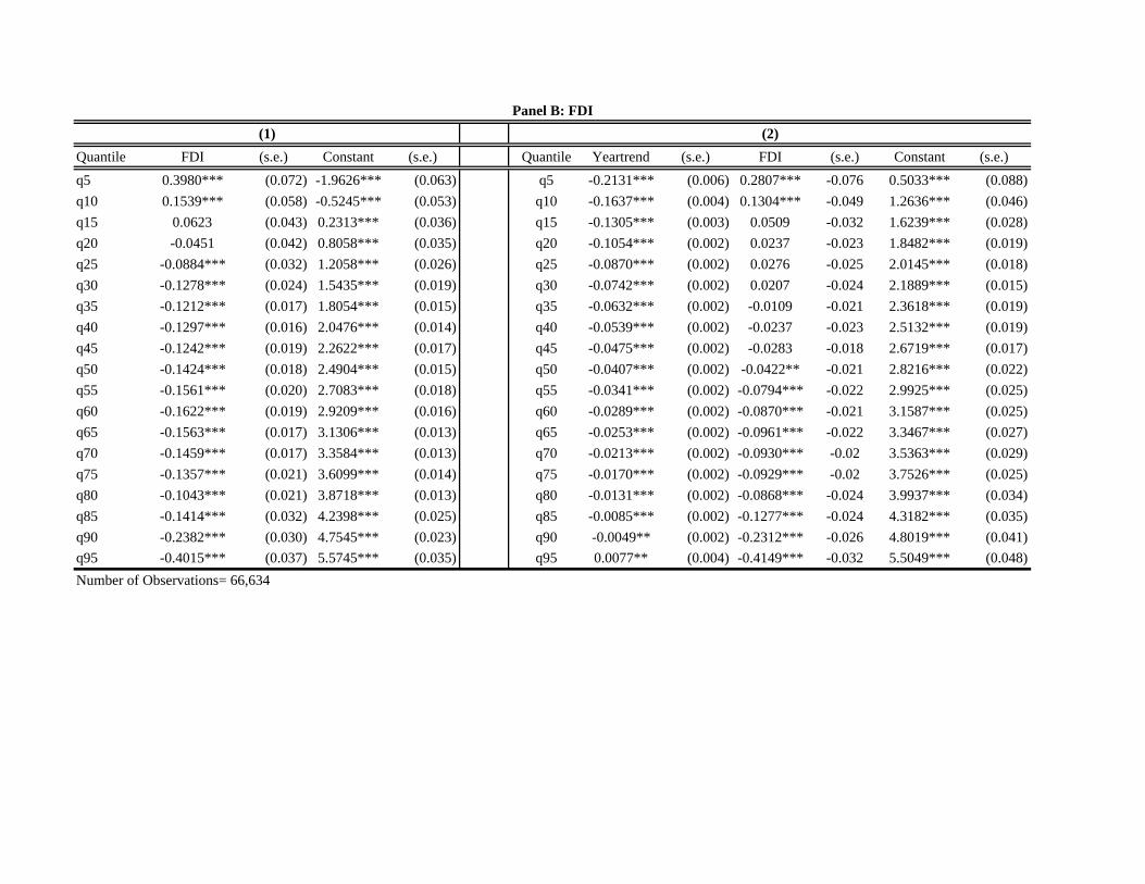
Quantile FDI (s.e.) Constant (s.e.) Quantile Yeartrend (s.e.) FDI (s.e.) Constant (s.e.)q5 0.3980*** (0.072) -1.9626*** (0.063) q5 -0.2131*** (0.006) 0.2807*** -0.076 0.5033*** (0.088) q10 0.1539*** (0.058) -0.5245*** (0.053) q10 -0.1637*** (0.004) 0.1304*** -0.049 1.2636*** (0.046) q15 0.0623 (0.043) 0.2313*** (0.036) q15 -0.1305*** (0.003) 0.0509 -0.032 1.6239*** (0.028) q20 -0.0451 (0.042) 0.8058*** (0.035) q20 -0.1054*** (0.002) 0.0237 -0.023 1.8482*** (0.019) q25 -0.0884*** (0.032) 1.2058*** (0.026) q25 -0.0870*** (0.002) 0.0276 -0.025 2.0145*** (0.018) q30 -0.1278*** (0.024) 1.5435*** (0.019) q30 -0.0742*** (0.002) 0.0207 -0.024 2.1889*** (0.015) q35 -0.1212*** (0.017) 1.8054*** (0.015) q35 -0.0632*** (0.002) -0.0109 -0.021 2.3618*** (0.019) q40 -0.1297*** (0.016) 2.0476*** (0.014) q40 -0.0539*** (0.002) -0.0237 -0.023 2.5132*** (0.019) q45 -0.1242*** (0.019) 2.2622*** (0.017) q45 -0.0475*** (0.002) -0.0283 -0.018 2.6719*** (0.017) q50 -0.1424*** (0.018) 2.4904*** (0.015) q50 -0.0407*** (0.002) -0.0422** -0.021 2.8216*** (0.022) q55 -0.1561*** (0.020) 2.7083*** (0.018) q55 -0.0341*** (0.002) -0.0794*** -0.022 2.9925*** (0.025) q60 -0.1622*** (0.019) 2.9209*** (0.016) q60 -0.0289*** (0.002) -0.0870*** -0.021 3.1587*** (0.025) q65 -0.1563*** (0.017) 3.1306*** (0.013) q65 -0.0253*** (0.002) -0.0961*** -0.022 3.3467*** (0.027) q70 -0.1459*** (0.017) 3.3584*** (0.013) q70 -0.0213*** (0.002) -0.0930*** -0.02 3.5363*** (0.029) q75 -0.1357*** (0.021) 3.6099*** (0.014) q75 -0.0170*** (0.002) -0.0929*** -0.02 3.7526*** (0.025) q80 -0.1043*** (0.021) 3.8718*** (0.013) q80 -0.0131*** (0.002) -0.0868*** -0.024 3.9937*** (0.034) q85 -0.1414*** (0.032) 4.2398*** (0.025) q85 -0.0085*** (0.002) -0.1277*** -0.024 4.3182*** (0.035) q90 -0.2382*** (0.030) 4.7545*** (0.023) q90 -0.0049** (0.002) -0.2312*** -0.026 4.8019*** (0.041) q95 -0.4015*** (0.037) 5.5745*** (0.035) q95 0.0077** (0.004) -0.4149*** -0.032 5.5049*** (0.048) Number of Observations= 66,634

(1) (2)Panel B: FDI

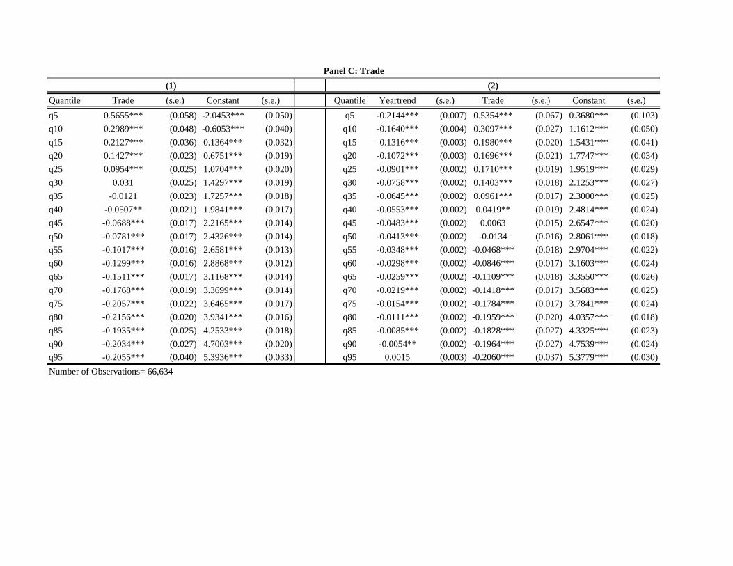
Quantile Trade (s.e.) Constant (s.e.) Quantile Yeartrend (s.e.) Trade (s.e.) Constant (s.e.)q5 0.5655*** (0.058) -2.0453*** (0.050) q5 -0.2144*** (0.007) 0.5354*** (0.067) 0.3680*** (0.103) q10 0.2989*** (0.048) -0.6053*** (0.040) q10 -0.1640*** (0.004) 0.3097*** (0.027) 1.1612*** (0.050) q15 0.2127*** (0.036) 0.1364*** (0.032) q15 -0.1316*** (0.003) 0.1980*** (0.020) 1.5431*** (0.041) q20 0.1427*** (0.023) 0.6751*** (0.019) q20 -0.1072*** (0.003) 0.1696*** (0.021) 1.7747*** (0.034) q25 0.0954*** (0.025) 1.0704*** (0.020) q25 -0.0901*** (0.002) 0.1710*** (0.019) 1.9519*** (0.029) q30 0.031 (0.025) 1.4297*** (0.019) q30 -0.0758*** (0.002) 0.1403*** (0.018) 2.1253*** (0.027) q35 -0.0121 (0.023) 1.7257*** (0.018) q35 -0.0645*** (0.002) 0.0961*** (0.017) 2.3000*** (0.025) q40 -0.0507** (0.021) 1.9841*** (0.017) q40 -0.0553*** (0.002) 0.0419** (0.019) 2.4814*** (0.024) q45 -0.0688*** (0.017) 2.2165*** (0.014) q45 -0.0483*** (0.002) 0.0063 (0.015) 2.6547*** (0.020) q50 -0.0781*** (0.017) 2.4326*** (0.014) q50 -0.0413*** (0.002) -0.0134 (0.016) 2.8061*** (0.018) q55 -0.1017*** (0.016) 2.6581*** (0.013) q55 -0.0348*** (0.002) -0.0468*** (0.018) 2.9704*** (0.022) q60 -0.1299*** (0.016) 2.8868*** (0.012) q60 -0.0298*** (0.002) -0.0846*** (0.017) 3.1603*** (0.024) q65 -0.1511*** (0.017) 3.1168*** (0.014) q65 -0.0259*** (0.002) -0.1109*** (0.018) 3.3550*** (0.026) q70 -0.1768*** (0.019) 3.3699*** (0.014) q70 -0.0219*** (0.002) -0.1418*** (0.017) 3.5683*** (0.025) q75 -0.2057*** (0.022) 3.6465*** (0.017) q75 -0.0154*** (0.002) -0.1784*** (0.017) 3.7841*** (0.024) q80 -0.2156*** (0.020) 3.9341*** (0.016) q80 -0.0111*** (0.002) -0.1959*** (0.020) 4.0357*** (0.018) q85 -0.1935*** (0.025) 4.2533*** (0.018) q85 -0.0085*** (0.002) -0.1828*** (0.027) 4.3325*** (0.023) q90 -0.2034*** (0.027) 4.7003*** (0.020) q90 -0.0054** (0.002) -0.1964*** (0.027) 4.7539*** (0.024) q95 -0.2055*** (0.040) 5.3936*** (0.033) q95 0.0015 (0.003) -0.2060*** (0.037) 5.3779*** (0.030) Number of Observations= 66,634

Panel C: Trade(1) (2)

(1b) (2b) (3b) (4b) (5b) (6b)Herfindahl Herfindahl Herfindahl Herfindahl Herfindahl Herfindahl(Sales) (Sales) (Sales) (Sales) (Sales) (Sales)

Delicence -0.0236** -0.0214**(0.01) (0.008)

FDI_LIB -0.0656*** -0.0510***(0.02) (0.013)

Trade_Lib -0.0739*** -0.0578***(0.025) (0.017)

Constant 0.1000*** 0.1356*** 0.1346*** 0.0946*** 0.1216*** 0.1210***(0.002) (0.012) (0.013) (0.002) (0.008) (0.009)

Observation 189,039 189,039 189,039 189,227 189,227 189,227R-squared 0.726 0.749 0.751 0.732 0.747 0.749

Table 8: Dergulation and Industry ConcentrationThis table presents regression estimates for an unbalanced panel of firms from 1989-1995. The dependent variable is the Herfindahl index of firm sales. Delicense is is a dummy variable that takes a value of 1 if a firm is an industry that delicensed entry in 1991. FDI_Lib and Trade_Lib are dummy variables that take a value of 1 if a firm is in an industry the liberlized to FDI or Trade in 1991. Clustered standard errors at the NIC3-digit industry-level in parentheses. *, ** and *** denote significance levels at 10%, 5% and 1%, respectively.

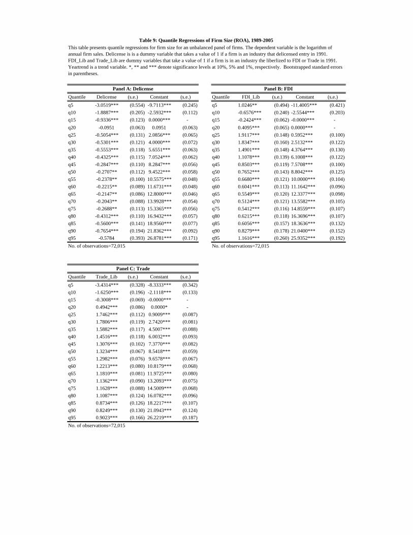
Quantile Delicense (s.e.) Constant (s.e.) Quantile FDI_Lib (s.e.) Constant (s.e.)q5 -3.0519*** (0.554) -9.7113*** (0.245) q5 1.0246** (0.494) -11.4005*** (0.421) q10 -1.8887*** (0.205) -2.5932*** (0.112) q10 -0.6576*** (0.240) -2.5544*** (0.203) q15 -0.9336*** (0.123) 0.0000*** - q15 -0.2424*** (0.062) -0.0000*** - q20 -0.0951 (0.063) 0.0951 (0.063) q20 0.4095*** (0.065) 0.0000*** - q25 -0.5054*** (0.131) 2.0856*** (0.065) q25 1.9117*** (0.148) 0.5952*** (0.100) q30 -0.5301*** (0.121) 4.0000*** (0.072) q30 1.8347*** (0.160) 2.5132*** (0.122) q35 -0.5553*** (0.118) 5.6551*** (0.063) q35 1.4901*** (0.148) 4.3764*** (0.130) q40 -0.4325*** (0.115) 7.0524*** (0.062) q40 1.1078*** (0.139) 6.1008*** (0.122) q45 -0.2847*** (0.110) 8.2847*** (0.056) q45 0.8503*** (0.119) 7.5708*** (0.100) q50 -0.2707** (0.112) 9.4522*** (0.058) q50 0.7652*** (0.143) 8.8042*** (0.125) q55 -0.2378** (0.100) 10.5575*** (0.048) q55 0.6680*** (0.121) 10.0000*** (0.104) q60 -0.2215** (0.089) 11.6731*** (0.048) q60 0.6041*** (0.113) 11.1642*** (0.096) q65 -0.2147** (0.086) 12.8000*** (0.046) q65 0.5549*** (0.120) 12.3377*** (0.098) q70 -0.2043** (0.088) 13.9928*** (0.054) q70 0.5124*** (0.121) 13.5582*** (0.105) q75 -0.2688** (0.113) 15.3365*** (0.056) q75 0.5412*** (0.116) 14.8559*** (0.107) q80 -0.4312*** (0.110) 16.9432*** (0.057) q80 0.6215*** (0.118) 16.3696*** (0.107) q85 -0.5600*** (0.141) 18.9560*** (0.077) q85 0.6056*** (0.157) 18.3636*** (0.132) q90 -0.7654*** (0.194) 21.8362*** (0.092) q90 0.8279*** (0.178) 21.0400*** (0.152) q95 -0.5784 (0.393) 26.8781*** (0.171) q95 1.1616*** (0.260) 25.9352*** (0.192) No. of observations=72,015 No. of observations=72,015

Quantile Trade_Lib (s.e.) Constant (s.e.)q5 -3.4314*** (0.328) -8.3333*** (0.342) q10 -1.6250*** (0.196) -2.1118*** (0.133) q15 -0.3008*** (0.069) -0.0000*** - q20 0.4942*** (0.086) 0.0000* - q25 1.7462*** (0.112) 0.9009*** (0.087) q30 1.7806*** (0.119) 2.7420*** (0.081) q35 1.5882*** (0.117) 4.5007*** (0.088) q40 1.4516*** (0.118) 6.0032*** (0.093) q45 1.3076*** (0.102) 7.3770*** (0.082) q50 1.3234*** (0.067) 8.5418*** (0.059) q55 1.2982*** (0.076) 9.6578*** (0.067) q60 1.2213*** (0.080) 10.8179*** (0.068) q65 1.1810*** (0.081) 11.9725*** (0.080) q70 1.1362*** (0.090) 13.2093*** (0.075) q75 1.1628*** (0.088) 14.5009*** (0.068) q80 1.1087*** (0.124) 16.0782*** (0.096) q85 0.8734*** (0.126) 18.2217*** (0.107) q90 0.8249*** (0.130) 21.0943*** (0.124) q95 0.9023*** (0.166) 26.2219*** (0.187) No. of observations=72,015

Panel A: Delicense Panel B: FDI

This table presents quantile regressions for firm size for an unbalanced panel of firms. The dependent variable is the logarithm of annual firm sales. Delicense is is a dummy variable that takes a value of 1 if a firm is an industry that delicensed entry in 1991. FDI_Lib and Trade_Lib are dummy variables that take a value of 1 if a firm is in an industry the liberlized to FDI or Trade in 1991. Yeartrend is a trend variable. *, ** and *** denote significance levels at 10%, 5% and 1%, respectively. Bootstrapped standard errors in parentheses.

Table 9: Quantile Regressions of Firm Size (ROA), 1989-2005

Panel C: Trade

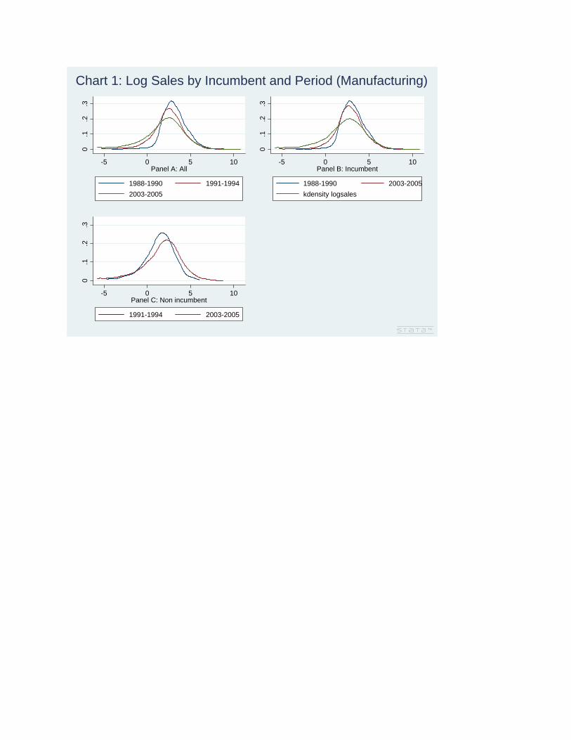
0.1

.2.3

-5 0 5 10Panel A: All

1988-1990 1991-1994

2003-2005

0.1

.2.3

-5 0 5 10Panel B: Incumbent

1988-1990 2003-2005

kdensity logsales

0.1

.2.3

-5 0 5 10Panel C: Non incumbent

1991-1994 2003-2005

Chart 1: Log Sales by Incumbent and Period (Manufacturing)

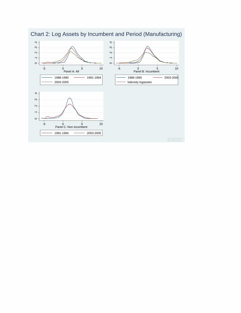
0.1

.2.3

.4

-5 0 5 10Panel A: All

1988-1990 1991-1994

2003-2005

0.1

.2.3

.4

-5 0 5 10Panel B: Incumbent

1988-1990 2003-2005

kdensity logassets

0.1

.2.3

.4

-5 0 5 10Panel C: Non incumbent

1991-1994 2003-2005

Chart 2: Log Assets by Incumbent and Period (Manufacturing)

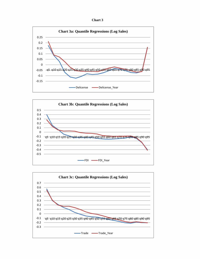
Chart 3

‐0.15

‐0.1

‐0.05

0

0.05

0.1

0.15

0.2

0.25

q5 q10 q15 q20 q25 q30 q35 q40 q45 q50 q55 q60 q65 q70 q75 q80 q85 q90 q95

Chart 3a: Quantile Regressions (Log Sales)

Delicense Delicense_Year

0 2‐0.1

00.10.20.30.40.5

q5 q10 q15 q20 q25 q30 q35 q40 q45 q50 q55 q60 q65 q70 q75 q80 q85 q90 q95

Chart 3b: Quantile Regressions (Log Sales)

‐0.15

‐0.1

‐0.05

0

0.05

0.1

0.15

0.2

0.25

q5 q10 q15 q20 q25 q30 q35 q40 q45 q50 q55 q60 q65 q70 q75 q80 q85 q90 q95

Chart 3a: Quantile Regressions (Log Sales)

Delicense Delicense_Year

‐0.5‐0.4‐0.3‐0.2‐0.1

00.10.20.30.40.5

q5 q10 q15 q20 q25 q30 q35 q40 q45 q50 q55 q60 q65 q70 q75 q80 q85 q90 q95

Chart 3b: Quantile Regressions (Log Sales)

FDI FDI_Year

‐0.3‐0.2‐0.1

00.10.20.30.40.50.60.7

q5 q10 q15 q20 q25 q30 q35 q40 q45 q50 q55 q60 q65 q70 q75 q80 q85 q90 q95

Chart 3c: Quantile Regressions (Log Sales)

Trade Trade_Year

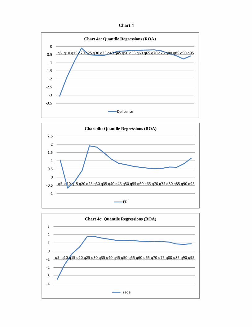
Chart 4

‐1

‐0.5

0

q5 q10 q15 q20 q25 q30 q35 q40 q45 q50 q55 q60 q65 q70 q75 q80 q85 q90 q95

Chart 4a: Quantile Regressions (ROA)

‐3

‐2.5

‐2

‐1.5

‐1

‐0.5

0

q5 q10 q15 q20 q25 q30 q35 q40 q45 q50 q55 q60 q65 q70 q75 q80 q85 q90 q95

Chart 4a: Quantile Regressions (ROA)

‐3.5

‐3

‐2.5

‐2

‐1.5

‐1

‐0.5

0

q5 q10 q15 q20 q25 q30 q35 q40 q45 q50 q55 q60 q65 q70 q75 q80 q85 q90 q95

Chart 4a: Quantile Regressions (ROA)

Delicense

2.5

Chart 4b: Quantile Regressions (ROA)

‐3.5

‐3

‐2.5

‐2

‐1.5

‐1

‐0.5

0

q5 q10 q15 q20 q25 q30 q35 q40 q45 q50 q55 q60 q65 q70 q75 q80 q85 q90 q95

Chart 4a: Quantile Regressions (ROA)

Delicense

0

0.5

1

1.5

2

2.5

Chart 4b: Quantile Regressions (ROA)

‐3.5

‐3

‐2.5

‐2

‐1.5

‐1

‐0.5

0

q5 q10 q15 q20 q25 q30 q35 q40 q45 q50 q55 q60 q65 q70 q75 q80 q85 q90 q95

Chart 4a: Quantile Regressions (ROA)

Delicense

‐1

‐0.5

0

0.5

1

1.5

2

2.5

q5 q10 q15 q20 q25 q30 q35 q40 q45 q50 q55 q60 q65 q70 q75 q80 q85 q90 q95

Chart 4b: Quantile Regressions (ROA)

FDI

Ch t 4 Q til R i (ROA)

‐3.5

‐3

‐2.5

‐2

‐1.5

‐1

‐0.5

0

q5 q10 q15 q20 q25 q30 q35 q40 q45 q50 q55 q60 q65 q70 q75 q80 q85 q90 q95

Chart 4a: Quantile Regressions (ROA)

Delicense

‐1

‐0.5

0

0.5

1

1.5

2

2.5

q5 q10 q15 q20 q25 q30 q35 q40 q45 q50 q55 q60 q65 q70 q75 q80 q85 q90 q95

Chart 4b: Quantile Regressions (ROA)

FDI

0

1

2

3

Chart 4c: Quantile Regressions (ROA)

‐3.5

‐3

‐2.5

‐2

‐1.5

‐1

‐0.5

0

q5 q10 q15 q20 q25 q30 q35 q40 q45 q50 q55 q60 q65 q70 q75 q80 q85 q90 q95

Chart 4a: Quantile Regressions (ROA)

Delicense

‐1

‐0.5

0

0.5

1

1.5

2

2.5

q5 q10 q15 q20 q25 q30 q35 q40 q45 q50 q55 q60 q65 q70 q75 q80 q85 q90 q95

Chart 4b: Quantile Regressions (ROA)

FDI

‐4

‐3

‐2

‐1

0

1

2

3

q5 q10 q15 q20 q25 q30 q35 q40 q45 q50 q55 q60 q65 q70 q75 q80 q85 q90 q95

Chart 4c: Quantile Regressions (ROA)

Trade

‐3.5

‐3

‐2.5

‐2

‐1.5

‐1

‐0.5

0

q5 q10 q15 q20 q25 q30 q35 q40 q45 q50 q55 q60 q65 q70 q75 q80 q85 q90 q95

Chart 4a: Quantile Regressions (ROA)

Delicense

‐1

‐0.5

0

0.5

1

1.5

2

2.5

q5 q10 q15 q20 q25 q30 q35 q40 q45 q50 q55 q60 q65 q70 q75 q80 q85 q90 q95

Chart 4b: Quantile Regressions (ROA)

FDI

‐4

‐3

‐2

‐1

0

1

2

3

q5 q10 q15 q20 q25 q30 q35 q40 q45 q50 q55 q60 q65 q70 q75 q80 q85 q90 q95

Chart 4c: Quantile Regressions (ROA)

Trade