Color Neutrality and the Gluon Distribution in a Very ... · In Sec. III we describe the conditions which the charge-density correlator must satisfy in order to be consistent with

arX

iv:h

ep-p

h/99

0728

1v3

23

Sep

1999

McGill/99–16hep-ph/9907281

Color Neutrality and the Gluon Distribution

in a Very Large Nucleus

C.S. Lam∗ and Gregory Mahlon†

Department of Physics, McGill University,

3600 University St., Montreal, QC H3A 2T8

Canada

(July 15, 1999)

Abstract

We improve the McLerran-Venugopalan model for the gluon distribution

functions in very large nuclei by imposing the condition that the nucleons

should be color neutral. We find that enforcing color neutrality cures the

infrared divergences in the transverse coordinates which are present in the

McLerran-Venugopalan model. Since we obtain well-defined expressions for

the distribution functions, we are able to draw unambiguous conclusions about

various features of the model. In particular, we show that the gluon distri-

bution functions in the absence of quantum corrections behave as 1/xF

to

all orders in the coupling constant. Furthermore, our distribution functions

exhibit saturation at small transverse momenta. The normalization of the

distribution function we obtain is not arbitrary but specified in terms of the

nucleon structure. We derive a sum rule for the integral of the gluon dis-

tribution function over transverse momenta, and show that the non-Abelian

contributions serve only to modify the shape of the transverse momentum

distribution. We obtain a relatively simple expression for the mean value of

the transverse momentum-squared. The connection between the McLerran-

Venugopalan model and the Dokshitzer-Gribov-Lipatov-Altarelli-Parisi equa-

tion is discussed quantitatively. Finally, we illustrate our results in terms of

a simple nuclear model due to Kovchegov.

24.85.+p, 12.38.Bx

Typeset using REVTEX

1

http://arxiv.org/abs/hep-ph/9907281v3

http://arxiv.org/abs/hep-ph/9907281

I. INTRODUCTION

Several years ago, McLerran and Venugopalan [1] recognized the existence of a regime inwhich the gluon structure functions ought to be calculable within quantum chromodynamics(QCD). Their idea is to recognize that in large nuclei at small enough values of the longi-tudinal momentum fraction x

F, the density of partons per unit area is large. Since a large

number of charges are contributing, it is expected that classical methods should apply, i.e.the vector potential is computed from the classical Yang-Mills equations, and quantum cor-relation functions are approximated by ensemble averages. This picture was developed morefully in subsequent work [2–4], and is somewhat related to the approach of Mueller [5–10].

In the region of very small xF, the quantum corrections to the distribution functions

calculated in the McLerran-Venugopalan model become large [4,11]. In particular, thesecorrections are enhanced by powers of αs ln(1/xF

), implying that the classical approximationbeing made at lowest order is breaking down in this region. This observation has lead to thedevelopment of a renormalization group procedure [12] whereby these corrections are takeninto account by incorporating gluons with large values of x

Finto the charge density. This

approach, which uses the results of the McLerran-Venugopalan model as its input, has beensubsequently developed in Refs. [12–18].

The focus of this paper is not on the very small xF

region, but rather on dealingwith the infrared divergence in the transverse coordinates which appears in the McLerran-Venugopalan model. The vector potential two-point correlation functions obtained inRef. [12] are highly infrared divergent, going like (x2)x

2

at large distances. On one hand, theregion where this poor behavior manifests itself is confined to separations x ≫ Λ−1

QCD. Thisis firmly in the non-perturbative regime where one does not really believe the results of aperturbative calculation anyway. However, since the gluon number density is derived fromthe Fourier transform of this correlation function, the presence of such a strong divergencemakes it difficult to obtain more than qualitative results from the theory: one must resortto cutting off the transverse spatial integrations at Λ−1

QCD [19].In this paper we will demonstrate that the infrared divergence described above is closely

related to the issue of color neutrality. Physically, nucleons appear to be colorless whenviewed at length scales which greatly exceed Λ−1

QCD. Consequently, we expect that two-

point correlation functions should die off rapidly beyond distance scales of about Λ−1QCD,

because of confinement. The quarks in two widely separated nucleons should not feel eachothers presence. Thus, the fundamental requirement that the nucleons be color neutral maybe rephrased as a restriction on the allowable charge-density correlation functions D(x).Although the McLerran-Venugopalan model employs an ensemble of charge distributionswhich respects the fact that the average charge should vanish, the two-point correlatorcomputed from this ensemble is inconsistent with color-neutral nucleons. We claim that thecolor neutrality condition should be viewed as of primary importance, and that we shouldmodify the ensemble of charge distributions to satisfy it. By doing so, we incorporateone of the major effects brought about by confinement, parameterizing it in terms of theprecise form chosen for D(x). Enforcing color neutrality cures the infrared divergence inthe McLerran-Venugopalan model by introducing a new scale into the problem, namelythe minimum length scale for which color neutrality holds. This outcome is somewhatsimilar to the one considered in Refs. [20,21]; however, neither of these papers examine the

2

consequences of enforcing color neutrality in great detail.Given a model which incorporates the color neutrality of the nucleons at some scale, we

obtain infrared finite correlation functions. Because our results are well-defined everywhere,we are able to draw firm conclusions about various properties of the gluon distribution func-tions, in spite of their highly nonlinear form. We are able to demonstrate that the gluondistribution functions in the McLerran-Venugopalan model are proportional to 1/x

F, inde-

pendent of the distribution of charge in the longitudinal coordinate. To evade this conclusionapparently requires charge-density correlation functions which have a non-trivial longitudi-nal structure. Although we have modified the form of D(x) from the one employed inRef. [12], we still obtain correlation functions which are consistent with asymptotic freedom.That is, in the ultraviolet limit, the non-Abelian terms drop out and we obtain a gluondistribution function which goes like 1/q2. At small values of the transverse momentumq, our gluon distribution functions either approach a finite constant or diverge mildly (likeln q2), depending on the long distance behavior of D(x). The density of gluons at smallq grows more slowly with increasing nuclear size than the number of nucleons, consistentwith saturation [10,22–24]. We also derive a transverse momentum sum rule, which showsthat the non-Abelian corrections only serve to transfer gluons (at fixed x

F) from one value of

transverse momentum to another: the total number of gluons is not altered. This is reflectedin the fact that the structure functions we obtain are simply proportional to the number ofnucleons: all non-linear dependence on the amount of charge present is suppressed at largevalues of the momentum transfer. As an application of the sum rule, we make contact withthe Dokshitzer-Gribov-Lipatov-Altarelli-Parisi equation [25,26], demonstrating the plausi-bility of the McLerran-Venugopalan model. In addition, we are able to compute a fairlysimple expression for the mean transverse momentum-squared of the gluons which is accu-rate to order unity: that is, the logarithms that arise in our calculation are all evaluatedat a scale which is completely calculable given a nucleon model. We find that the leadingQ2 behavior of this quantity is linear in the number of nucleons, whereas the logarithmiccorrections are quadratic in the charge per unit transverse area.

The remainder of this paper is organized as follows. In Sec. II, we review the McLerran-Venugopalan model as described in Refs. [1–4,12]. We allow for a generalized dependenceof the charge-density correlator on the transverse coordinates in order to set the stage forthe subsequent discussion. In Sec. III we describe the conditions which the charge-densitycorrelator must satisfy in order to be consistent with nucleons which are color neutral. Weexamine the properties of the resulting gluon number density in Sec. IV. If the charge-density correlator is Gaussian and local in the longitudinal coordinate, we show that thegluon number density is always proportional to 1/x

F. We derive a sum rule for the integral

of the gluon number density over the transverse momenta, and apply it to the computationof the gluon distribution function at large values of the momentum transfer. Our result isclosely related to the Dokshitzer-Gribov-Lipatov-Altarelli-Parisi equation. Sec. IV concludeswith a discussion of the mean value of the transverse momentum-squared obtained by ourapproach. We illustrate our results in Sec. V within the context of a specific nuclear model byKovchegov [27]. Finally, Sec. VI contains our conclusions. A discussion of our notation andconventions may be found in Appendix A. The details of how to evaluate various integralsarising in the text are contained in Appendices B, C, and D.

3

II. REVIEW OF THE MCLERRAN-VENUGOPALAN MODEL

A. General Considerations

The goal of the McLerran-Venugopalan (MV) model is to compute the gluon distribu-tion function at small values of the longitudinal momentum fraction x

F≡ q+gluon/Q

+nucleon

for a very large nucleus. We begin our discussion with the assumptions which form thebasis of the MV model, and outline the steps in the computation of the gluon distributionfunction. Having described the ingredients which underlie the calculations, we will explainthe conditions which are required for this picture to be applicable.

Consider a nucleus moving along the z axis at nearly the speed of light. The centralassertion of the MV model is that, in a specific kinematic regime, we may determine thegluon distribution function of the nucleus as follows. First, we are told to compute theclassical vector potential generated by the valence quarks. Since the valence quarks appearas a Lorentz-contracted pancake-shaped distribution of color charge, the current appearingin the classical Yang-Mills equations takes the form (see Appendix A for a summary of ournotation and conventions)

J+(x) = ρ(x−,x),J−(x) = 0,J(x) = 0. (2.1)

There is no x+ dependence in Eq. (2.1) in the limit that the source (i.e. the nucleus) ismoving at the speed of light. Because the intuitive parton model is realized in the light-conegauge [28–31], we should write the solution in that gauge, i.e. A+ ≡ 0.

By definition, the gluon number density is just the gluon number operator evaluated inthe (quantum) state of interest. This may be expressed in terms of the two-point vectorpotential correlation function as [23,29]

dN

dq+d2q=

q+

4π3

∫ ∞

−∞dx−

∫d2x

∫ ∞

−∞dx′−

∫d2x′ e−iq+(x−−x′−)eiq·(x−x′)〈Aa

i (x−,x)Aa

i (x′−,x′)〉.

(2.2)

In the MV model, the average over quantum fluctuations implied by the angled bracketson the right hand side of (2.2) is replaced by a classical average over a suitably weightedensemble of charge densities. The ensemble should consist of all of the physically realizablestates of the quarks (in color singlet combinations) within the nucleons and of the nucleonswithin the nucleus. Then, what we require is an expression for the vector potential in termsof the charge density plus the probability distribution for determining how likely a givencharge configuation is. In the MV model, ensemble averages are computed according to theGaussian weight

∫[dρ] exp

−

∫dx− d2x

∫dx′− d2x′ Tr

[ρ(x−,x)ρ(x′−,x′)

]δ(x− − x′− )

µ2(x−)D−1(x− x′)

. (2.3)

This weight implies that the charge density has an average value of zero. There are, however,fluctuations about this average value, the size of which are governed by µ2(x−), which is

4

related to the average charge density squared per unit area per unit thickness.1 The precisestatement of the relationship appears in Sec. III. The longitudinal dependence of Eq. (2.3) ispurely local in x−, reflecting the fact that the large number of quarks which contribute to thecharge per unit area at a given transverse position typically come from different nucleons:hence, they should be uncorrelated. The transverse space dependence of the MV model asdescribed in Refs. [1–4,12] is

D(x− x′) = δ2(x− x′). (2.4)

Ultimately, we intend to modify this dependence. Therefore, we will write our expressions interms of D and insert (2.4) only when we wish to specifically discuss the results of Ref. [12].

Thus, given the solution for the vector potential in terms of the charge density and anansatz for the charge density correlation function, we may compute an approximation to thegluon distribution function. We now describe the conditions necessary for this procedure toyield a good approximation to the result which would be obtained in a full QCD treatment.

First, we note that the charge distribution for the nucleus is taken to be a Lorentz-contracted pancake moving along the z axis at (nearly) the speed of light. We wish to bein the regime where the partons do not resolve its longitudinal structure. This is only truefor partons with very small longitudinal momentum fractions. To determine how small themomentum should be, we note that the corresponding length scale x− ∼ 1/q+gluon shouldbe larger than the thickness of the Lorentz-contracted nucleus. This thickness is of orderA1/3a/γ, where A is the number of nucleons, a the radius of a single nucleon, and γ is the(common) boost factor of the nucleons which comprise the nucleus. Writing the mass of thenucleon to be m, we see then that the condition on the momentum fraction reads

xF≡ q+gluonQ+

nucleon

<∼A−1/3

ma. (2.5)

Gluons with longitudinal momenta satisfying (2.5) cannot resolve distances shorter than thethickness of the Lorentz-contracted nucleus they see.

An immediate consequence of being unable to resolve nucleons with different values ofx− is that we may view the nucleons as being piled up onto effectively the same value ofx−. Thus, each unit of transverse area will, on average, contain a large number of valencequarks. Since there are a large number of quarks contributing, the total contribution willbe in a large representation of the gauge group, allowing us to treat the source in the theclassical approximation. The large number of quarks also allows us to justify the use of theGaussian weight (2.3) via the central limit theorem. The number of valence quarks per unitarea in a flattened nucleus of radius R is 3A/πR2 ∼ 3A1/3/πa2, since the nuclear radiusscales with the number of nucleons as R ∼ A1/3a. Gluons with a transverse momentum q2

1The authors of Ref. [12] choose to replace the spatial variable x− with what they call the space-

time rapidity y, defined by y ≡ y0 + ln(x−0 /x−). Thus, they write µ2(y) and refer to it as the

average charge density squared per unit area per unit rapidity. We will stick to the description in

terms of x− in this paper.

5

see a transverse area of about π/q2. Thus, to maintain the condition that there is a largenumber of quarks in the region being probed, we should only look at transverse momentasuch that

Λ2QCD

<∼ q2 <∼ 3A1/3a−2, (2.6)

that is, q should be soft enough to correspond to a large enough area, but not so soft thatthe coupling becomes strong. A second factor limiting the maximum q2 for which thistreatment is valid is the observation that if the transverse momentum of the emitted gluonsis too large, then the eikonal approximation we are making breaks down. That is, the no-recoil approximation that allowed us to treat the valence quarks as being localized on thelight-cone fails.

The bottom line is that in large enough nuclei for small enough values of the longitudinalmomentum carried by the parton and moderately large tranverse momenta, the number ofquarks per unit area becomes large. In this regime, we expect that we may compute thegluon distribution function at lowest order from the classical solution to the Yang-Millsequations.

B. Non-Abelian Weisacker-Williams Fields

As outlined above, the MV model makes use of the classical solution to the Yang-Millsequations in the presence of a source of the form (2.1), with J+(x) ≡ ρ(x−,x) the onlynonzero component, independent of the light-cone time x+. Ultimately, we will take the de-pendence on the light-cone distance x− to be a delta function, corresponding to the pancake-shaped distribution described above. Initially, however, we will work with a finite spread inx− (a multi-layer pancake), to avoid the ambiguities that would otherwise arise in the com-mutator terms of the Yang-Mills equations [12]. Furthermore, certain quantum correctionsmay be included by a renormalization group treatment [12–18] which generates a specific x−

dependence, reflecting the presence of the Yukawa cloud of quark pairs and gluons aroundthe original source. So, it behooves us to make provision for such a dependence.

The simplest route to the solution for the vector potential in the light-cone gauge fora current of the form (2.1) is to begin by finding the solution in the covariant gauge, andsubsequently transform into the light-cone gauge [5,27]. Therefore, we begin in the covariantgauge, ∂µA

µ(x) = 0, where the field equations (A3) become

∂2Aν − 2i[Aµ, ∂µA

ν]+ i

[Aµ, ∂

νAµ]−

[Aµ,

[Aµ, Aν

]]= Jν . (2.7)

We recall that in electrodynamics, the µth component of the vector potential is generatedby the µth component of the current (in the covariant gauge). Analogously, we attempt toform a solution where the only non-zero component is A+. Imposing this condition, we findthat this is possible, provided that

∂2A+ − 2i[A+, ∂+A

+]= ρ. (2.8)

Since A− and Ai vanish, the condition that we are in covariant gauge reduces to ∂+A+ = 0.

Hence A+ is independent of x+ and Eq. (2.8) reduces to

6

∇2A+(x−,x) = ρ(x−,x), (2.9)

Notice that Eq. (2.9) is local in x−. This is a consequence of the x+-independence of thevector potential, which reduces ∂2 = −2∂+∂− +∇

2 to just ∇2. The solution of (2.9) is

A+(x−,x) =∫d2x′G(x− x′)ρ(x−,x′), (2.10)

where

G(x− x′) ≡ 1

4πln( |x− x′|2

λ2

). (2.11)

The arbitrary length scale λ which appears in (2.11) reflects the lack of a scale in the classicaltheory. This same lack of scale leads to the infrared divergence in perturbation theory. Notethat in the covariant gauge, the fact that J and A are color matrices has introduced no realcomplications into the solution: the vector potential is still linear in the sources.

The non-Abelian features make themselves felt when we gauge transform our solution tothe light-cone gauge. We write the gauge transformation as

Aµ(x) = U(x)Aµ(x)U−1(x)− i[∂µU(x)

]U−1(x). (2.12)

Asking that the new gauge be the light-cone gauge, A+ ≡ 0, we find that U(x) should satisfy

i[∂−U(x)

]= U(x)A+(x). (2.13)

The solution to Eq. (2.13) is the path-ordered exponential

U(x) ≡ P exp

[i∫ x−

−∞dξ− A+(ξ−,x)

], (2.14)

where the sense of the path-ordering P is such that

U(x) ≡ 1+∞∑

j=1

ij∫ x−

−∞dξ−1

∫ ξ−1

−∞dξ−2 · · ·

∫ ξ−j−1

−∞dξ−j A+(ξ−j ,x) · · · A+(ξ−2 ,x)A

+(ξ−1 ,x), (2.15)

i.e. the factors are arranged such that x− increases as the factors of A+ are read from leftto right. Using (2.12) and (2.14) to obtain the light-cone gauge expressions yields

A−(x) = 0 (2.16)

and

Aj(x) = −i[∂jU(x)

]U−1(x)

=∫ x−

−∞dξ− U(ξ−,x)

[∂jA+(ξ−,x)

]U−1(ξ−,x). (2.17)

The Abelian limit may be obtained from Eq. (2.17) by allowing all quantities to commute.Equivalently, we may take only those contributions which are linear in the source.

7

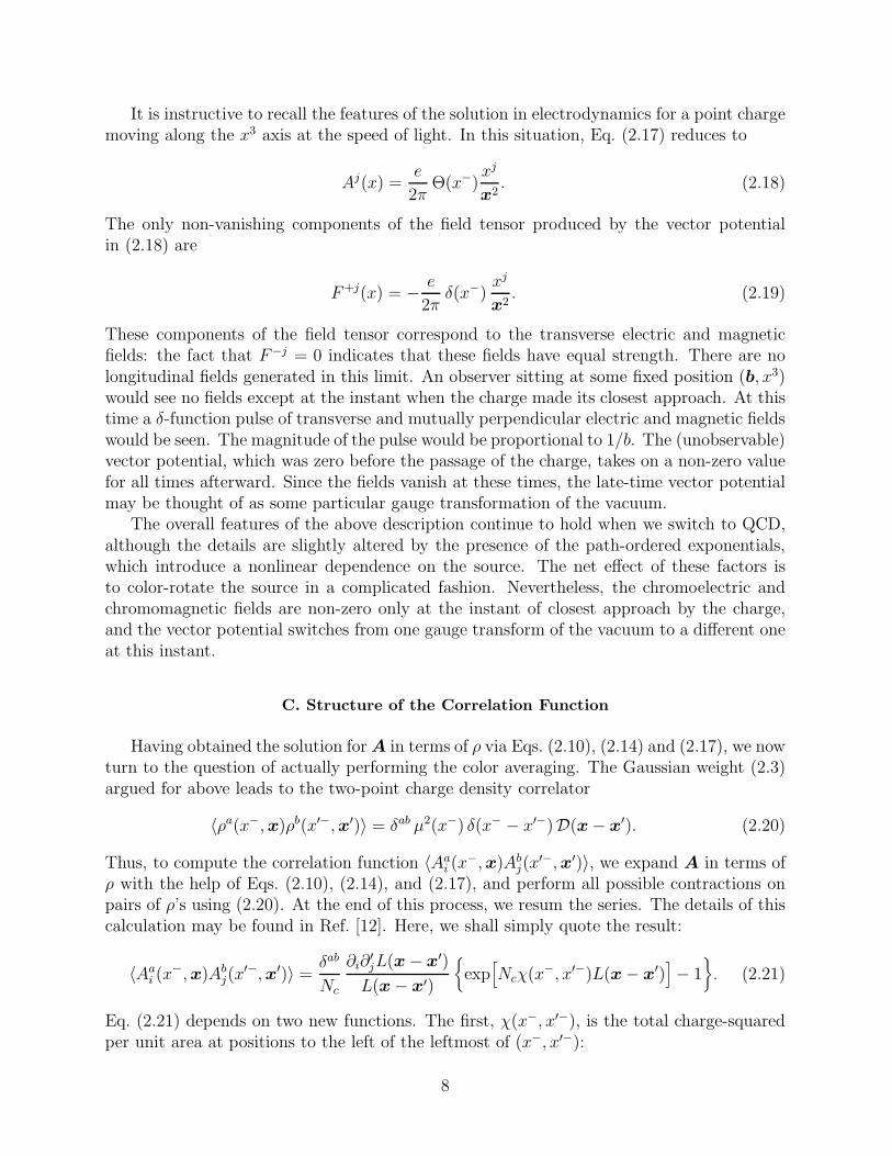
It is instructive to recall the features of the solution in electrodynamics for a point chargemoving along the x3 axis at the speed of light. In this situation, Eq. (2.17) reduces to

Aj(x) =e

2πΘ(x−)

xj

x2. (2.18)

The only non-vanishing components of the field tensor produced by the vector potentialin (2.18) are

F+j(x) = − e

2πδ(x−)

xj

x2. (2.19)

These components of the field tensor correspond to the transverse electric and magneticfields: the fact that F−j = 0 indicates that these fields have equal strength. There are nolongitudinal fields generated in this limit. An observer sitting at some fixed position (b, x3)would see no fields except at the instant when the charge made its closest approach. At thistime a δ-function pulse of transverse and mutually perpendicular electric and magnetic fieldswould be seen. The magnitude of the pulse would be proportional to 1/b. The (unobservable)vector potential, which was zero before the passage of the charge, takes on a non-zero valuefor all times afterward. Since the fields vanish at these times, the late-time vector potentialmay be thought of as some particular gauge transformation of the vacuum.

The overall features of the above description continue to hold when we switch to QCD,although the details are slightly altered by the presence of the path-ordered exponentials,which introduce a nonlinear dependence on the source. The net effect of these factors isto color-rotate the source in a complicated fashion. Nevertheless, the chromoelectric andchromomagnetic fields are non-zero only at the instant of closest approach by the charge,and the vector potential switches from one gauge transform of the vacuum to a different oneat this instant.

C. Structure of the Correlation Function

Having obtained the solution forA in terms of ρ via Eqs. (2.10), (2.14) and (2.17), we nowturn to the question of actually performing the color averaging. The Gaussian weight (2.3)argued for above leads to the two-point charge density correlator

〈ρa(x−,x)ρb(x′−,x′)〉 = δab µ2(x−) δ(x− − x′−)D(x− x′). (2.20)

Thus, to compute the correlation function 〈Aai (x

−,x)Abj(x

′−,x′)〉, we expand A in terms ofρ with the help of Eqs. (2.10), (2.14), and (2.17), and perform all possible contractions onpairs of ρ’s using (2.20). At the end of this process, we resum the series. The details of thiscalculation may be found in Ref. [12]. Here, we shall simply quote the result:

〈Aai (x

−,x)Abj(x

′−,x′)〉 = δab

Nc

∂i∂′jL(x− x′)

L(x− x′)

exp

[Ncχ(x

−, x′−)L(x− x′)]− 1

. (2.21)

Eq. (2.21) depends on two new functions. The first, χ(x−, x′−), is the total charge-squaredper unit area at positions to the left of the leftmost of (x−, x′−):

8

χ(x−, x′−) ≡∫ min(x−,x′−)

−∞dξ− µ2(ξ−). (2.22)

The appearance of such an expression is not surprising when we recall that the value of thevector potential depends on whether or not the charge has yet reached its point of closestapproach. What χ(x−, x′−) measures is the amount of charge in those layers of the sourcewhich have already passed both of the points which we are comparing. Although the rangeof integration extends to x− = −∞, in practice this is cut off by the form of µ2(x−), whichfor a pancake-shaped charge distribution, should be non-zero only in a relatively small rangearound the position of the nucleus along the x− axis.

The second new function appearing in (2.21) is given by

L(x− x′) ≡∫d2ξ

∫d2ξ′D(ξ − ξ′)

[G(x− ξ)G(x′ − ξ′)− 1

2G(x− ξ)G(x− ξ′)

− 12G(x′ − ξ)G(x′ − ξ′)

]. (2.23)

Note that this function vanishes when x = x′. Thus, at very short distances the nonlinearterms in (2.21) drop out and the behavior of the correlation function is the same as in theAbelian case:

lim|x−x′|→0

〈Aai (x

−,x)Abj(x

′−,x′)〉 = δabχ(x−, x′−)[∂i∂

′jL(x− x′)

]. (2.24)

In this limit, all of the dependence on the transverse coordinates is contained in the derivativeof L:

∂i∂′jL(x− x′) =

∫d2ξ

∫d2ξ′D(ξ − ξ′)[∂iG(x− ξ)][∂jG(x

′ − ξ′)]

≡ δijL(x− x′) + Lij(x− x′). (2.25)

To uniquely specify the decomposition appearing on the second line of (2.25) we take Lij tobe traceless. Hence, the only piece of (2.25) which contributes to the gluon number densityis δijL(x− x′).

D. Result Assuming Purely Local Charge Density Correlations

As mentioned earlier, the results presented in Ref. [12] utilize a purely local correlator forthe charge density correlation function, i.e. Eq. (2.4). Inserting such a δ-function dependenceinto (2.23) produces

L(x− x′) = γ(x− x′)− γ(0) (2.26)

where, formally,2

2The authors of Ref. [12] write γ(x) = 1∇4 δ

2(x), whereas we obtain the convolution of 1∇2 δ

2(x)

with itself. To demonstrate the equivalence of these two quantities requires that we employ a

consistent regularization scheme for the infrared divergences, for example by doing the entire

computation in 2 + ε dimensions.

9

γ(x− x′) =∫d2ξG(x− ξ)G(x′ − ξ). (2.27)

This function contains a quadratic infrared divergence, on top of the arbitrary length scaleintroduced by the logarithmic divergence of G(x − x′) itself. Fortunately, it is only thecombination γ(x−x′)−γ(0) which appears in the correlation function. Thus, the quadraticpart of the divergence drops out. There is still a logarithmic dependence on the infraredcutoff. The authors of Ref. [12] take3

γ(x− x′)− γ(0) =1

16π|x− x′|2 ln

(|x− x′|2Λ2

QCD

)(2.28)

where they have chosen on physical grounds to set this cutoff to Λ−1QCD. The derivative

of (2.28) is

∂i∂′jγ(x− x′) = − δij

8π

[ln(|x− x′|2Λ2

QCD

)+ 2

]

+1

4π

[1

2δij −

(x− x′)i(x− x′)j|x− x′|2

]. (2.29)

Note that the terms on the second line of (2.29) are traceless, and do not contribute to thegluon number density (2.2).

Because γ(x−x′) is formally the inverse of∇4, when we form the trace ∂i∂′iγ(x−x′) that

appears in (2.21), we should obtain the inverse of ∇2 [i.e. Eq. (2.11)]. Eq. (2.29) satisfiesthis expectation, since the extra “+2” appearing in the first line may be absorbed into thearbitrary scale. What this means is that in a strict evaluation of Eq. (2.21), if we want thenumerator factor ∂i∂

′jγ(x− x′) to consist of a single logarithmic term, then that logarithm

must contain a different scale from the one used in L(x − x′) itself. On the other hand, inthe qualitative treatment of the infrared employed in Ref. [12], both logarithms are assumedto have the same scale (∼ ΛQCD), producing

〈Aai (x

−,x)Aai (x

′−,x′)〉 = 4(N2c − 1)

Nc|x− x′|2[1−

(|x− x′|2Λ2

QCD

)(Nc/16π)χ(x− ,x′−)|x−x′|2]. (2.30)

According to Eq. (2.2), the gluon number density depends on the Fourier transform of (2.30).Unfortunately, there is a problem with the correlation function appearing in Eq. (2.30): itdiverges like (x2)x

2

at large distances. Thus, the required Fourier transform does not exist

for any value of the momentum q! In Ref. [19], the x − x′ integration is cut off at Λ−1QCD,

on the grounds that the approximations made in obtaining (2.30) are not valid at largedistances. While physically reasonable, such an approach can only be applied qualitatively.

It is apparent from the discussion leading to Eq. (2.24) that Eq. (2.30) neverthelesscorrectly reproduces the Abelian limit at short enough distances. Explicitly,

3This expression for γ differs from the one given in Eq. (26) of Ref. [12] by a factor of 2. This is

in agreement with the requirement ∇2γ(x) = 1∇2 δ

2(x).

10

lim|x−x′|→0

〈Aai (x

−,x)Aai (x

′−,x′)〉 = N2c − 1

4πχ(x−, x′−) ln

(|x− x′|2Λ2

QCD

). (2.31)

The Fourier transform of this function goes like 1/q2.At larger distances, 0 ≪ |x − x′| ≪ Λ−1

QCD, and for large enough nuclei, the secondterm of (2.30) becomes negligible. Under these circumstances, the correlation function hasa Fourier transform which behaves as ln q2. To see how large the nucleus has to be to havesuch a regime, consider the function f(ξ) ≡ ξΩξ. It has a minimum at ξ = e−1, independentof Ω, and a minimum value of e−Ω/e. Thus, to legitimately drop the second term of (2.30)we should have

Ω =Ncχ

16πΛ2QCD

≫ e. (2.32)

This constraint is difficult to satisfy: in fact, for experimentally accessible nuclei, such asuranium, we actually have Ω < 1. Just to obtain Ω ∼ e requires χ ∼ 45Λ2

QCD. For themodel described in Sec. V, this implies a nucleus with of order 105 nucleons. This is asomewhat larger nucleus than is required simply to make the color charge density largeenough for the approximations described at the beginning of this section to be reasonable[compare Eqs. (2.6) and (2.32)]. So while the authors of Refs. [1–4,12,19] point out thatrealistic nuclei are only marginally large enough, one must go to even larger nuclei to justifydropping the second term in (2.30).

Our point is, that the range of momenta where the picture described at the beginningof this section and in Refs. [12,19,23] is applicable is very narrow at best. While it isunlikely that anything short of a full non-perturbative solution to QCD can produce reliablepredictions for the region |x − x′| >∼ Λ−1

QCD, we may reasonably hope that if we constructa model which is well-behaved in this region, then we will be able to trust it closer to theboundary point |x−x′| = Λ−1

QCD than if we use Eq. (2.30), with its unphysical large-distancebehavior. In the next section we will show that the source of the difficulties encounteredin Eq. (2.30) is the inconsistency of the charge density correlator (2.20) with the intuitivepicture of color neutral nucleons. When the correlator is altered to reflect this expectation,we find that the resulting gluon distribution is well-behaved and completely infrared finite.

III. COLOR NEUTRALITY

As described in the previous section, the MV model employs the Gaussian weight (2.3) forperforming ensemble averages. Thus, the ensemble average of the charge denisty vanishes [1]:

〈ρa(x−,x)〉 = 0. (3.1)

This says that at any given point, when averaging over all of the different nuclei within theensemble, we see no net charge. Eq. (3.1) is gauge-invariant in the sense that if we performthe same gauge transformation on the fields present in all of the nuclei, the ensemble averageremains unchanged.

Let us consider the situation inside a single hadronic state, which we will denote by|h〉. This state could consist of a single baryon or meson, or it could be some collection ofhadrons. For such a state, the charge density at a given point is not necessarily zero:

11

〈h| ρa(x−,x) |h〉 6= 0. (3.2)

However, if we sum over all of the space occupied by the hadronic state, we should obtainzero:

〈h|∫dx−d2x ρa(x−,x) |h〉 = 0. (3.3)

Eq. (3.3) says that any physically observable hadronic state is a color singlet. Since this istrue for all of the hadronic states in our Hilbert space, we may use the polarization trick togeneralize (3.3) to

〈h|∫dx−d2x ρa(x−,x) |h′〉 = 0. (3.4)

Since we have phrased Eq. (3.4) in terms of color singlet physical states, it must holdindependent of the gauge chosen for ρa(x−,x).

Now consider the bilinear combination

Z ≡ 〈h|∫dx−d2x

∫dx′−d2x′ ρa(x−,x)ρb(x′−,x′) |h〉. (3.5)

On one hand, by inserting a complete set of hadronic states and applying Eq. (3.4) weconclude that Z vanishes. Since the ensemble utilized in the MV model consists of a specificcollection of hadronic states (i.e. nuclei with some fixed number of nucleons), we furtherconclude that the ensemble average of Z vanishes. On the other hand, we may also computethe ensemble average of Z with the help of the correlation function (2.20):

〈Z〉 =∫dx−d2x

∫dx′−d2x′ 〈ρa(x−,x)ρb(x′−,x′)〉

= δab∫d2Σ

∫ ∞

−∞dx− µ2(x−)

∫d2∆D(∆). (3.6)

The integral over Σ is just the (non-zero) transverse area of the nucleus. Since µ2(x−) ispositive (by definition), the only way to obtain a vanishing ensemble average is to requirethat D satisfy

∫d2∆D(∆) = 0. (3.7)

This relation is not true for the choice (2.4) employed in Ref. [12]. Hence we concludethat this choice is incompatible with the expectation of color-neutral nucleons. In fact, thisviolation of color-neutrality contributes to the poor infrared behavior of the MV correlationfunction (2.30).

Although the function D(∆) is itself not gauge-invariant (its transformation propertiesare determined by the condition that the Gaussian weight be gauge-invariant), the color-neutrality condition (3.7) was, nonetheless, derived in a gauge-invariant fashion, with thehelp of Eq. (3.4). The constraint represented by Eq. (3.7) reflects the physical observationthat the nucleus does not carry a net color charge.

The fact that a color neutral charge distribution posseses an intrinsic scale explains whythe infrared behavior of the gluon number density is improved by enforcing (3.7). We may

12

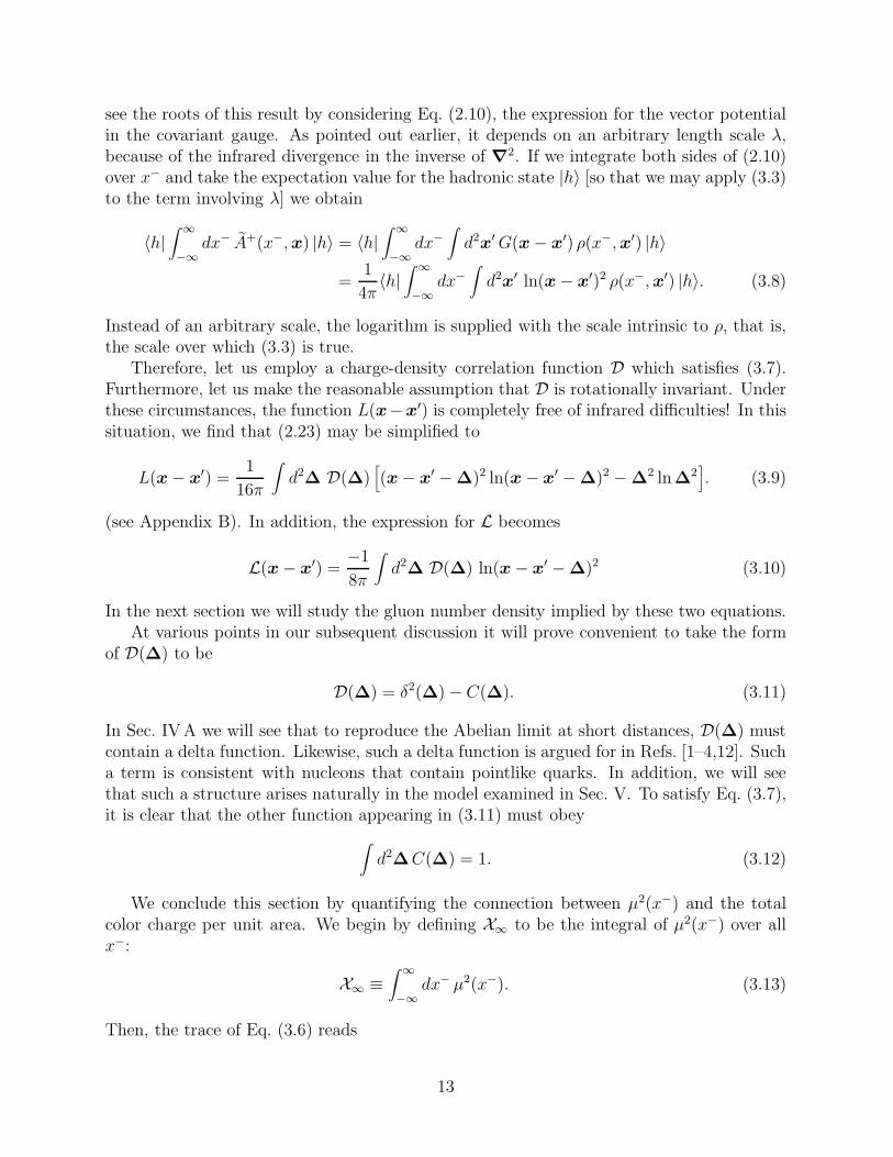
see the roots of this result by considering Eq. (2.10), the expression for the vector potentialin the covariant gauge. As pointed out earlier, it depends on an arbitrary length scale λ,because of the infrared divergence in the inverse of ∇2. If we integrate both sides of (2.10)over x− and take the expectation value for the hadronic state |h〉 [so that we may apply (3.3)to the term involving λ] we obtain

〈h|∫ ∞

−∞dx− A+(x−,x) |h〉 = 〈h|

∫ ∞

−∞dx−

∫d2x′G(x− x′) ρ(x−,x′) |h〉

=1

4π〈h|

∫ ∞

−∞dx−

∫d2x′ ln(x− x′)2 ρ(x−,x′) |h〉. (3.8)

Instead of an arbitrary scale, the logarithm is supplied with the scale intrinsic to ρ, that is,the scale over which (3.3) is true.

Therefore, let us employ a charge-density correlation function D which satisfies (3.7).Furthermore, let us make the reasonable assumption that D is rotationally invariant. Underthese circumstances, the function L(x−x′) is completely free of infrared difficulties! In thissituation, we find that (2.23) may be simplified to

L(x− x′) =1

16π

∫d2∆ D(∆)

[(x− x′ −∆)2 ln(x− x′ −∆)2 −∆2 ln∆2

]. (3.9)

(see Appendix B). In addition, the expression for L becomes

L(x− x′) =−1

8π

∫d2∆ D(∆) ln(x− x′ −∆)2 (3.10)

In the next section we will study the gluon number density implied by these two equations.At various points in our subsequent discussion it will prove convenient to take the form

of D(∆) to be

D(∆) = δ2(∆)− C(∆). (3.11)

In Sec. IVA we will see that to reproduce the Abelian limit at short distances, D(∆) mustcontain a delta function. Likewise, such a delta function is argued for in Refs. [1–4,12]. Sucha term is consistent with nucleons that contain pointlike quarks. In addition, we will seethat such a structure arises naturally in the model examined in Sec. V. To satisfy Eq. (3.7),it is clear that the other function appearing in (3.11) must obey

∫d2∆C(∆) = 1. (3.12)

We conclude this section by quantifying the connection between µ2(x−) and the totalcolor charge per unit area. We begin by defining X∞ to be the integral of µ2(x−) over allx−:

X∞ ≡∫ ∞

−∞dx− µ2(x−). (3.13)

Then, the trace of Eq. (3.6) reads

13

∫dx−d2x

∫dx′−d2x′ 〈ρa(x−,x)ρa(x′−,x′)〉 = (N2

c − 1)X∞πR2∫d2∆D(∆). (3.14)

Imagine that, instead of a color-neutral distribution of charge satisfying (3.7), we considera single quark. Then, it would indeed be true that D(∆) = δ2(∆), and the charge-squaredof that quark should be given by

g2CF ≡ (N2c − 1)X∞πR

2 (3.15)

where CF = (N2c − 1)/2Nc is the Casimir factor for SU(N). Thus, we see that the color

charge squared per unit area is (N2c − 1)X∞, and that the precise meaning of µ2(x−) is

actually the charge squared per unit area per unit thickness divided by N2c − 1.

IV. GLUON NUMBER DENSITY

We begin our discussion of the properties of the gluon number density resulting from anucleus consisting of color-neutral nucleons by inserting (2.21) into the master formula (2.2).Employing sum and difference variables for the transverse integrations we obtain

dN

dq+d2q=

q+

2π3

N2c − 1

Nc

∫d2Σ

∫d2∆ eiq·∆

L(∆)

L(∆)

×∫ ∞

−∞dx−

∫ ∞

−∞dx′−e−iq+(x−−x′−)

exp

[Ncχ(x

−, x′−)L(∆)]− 1

. (4.1)

The result of the Σ integration appearing in Eq. (4.1) should be interpreted as πR2, thetransverse area of the Lorentz-contraced nucleus.4 We would like to perform the transverseintegrations. All of the longitudinal dependence is contained in the function χ(x−, x′−).

Recall that within the Gaussian ansatz (2.3), the function χ(x−, x′−) is given by

χ(x−, x′−) ≡∫ min(x−,x′−)

−∞dξ− µ2(ξ−). (4.2)

In order to obtain a more useful expression for χ, let us define

X (x−) ≡∫ x−

−∞dξ− µ2(ξ−). (4.3)

Then, we see that Eq. (4.2) has the form

χ(x−, x′−) = X (x−)Θ(x′− − x−) + X (x′−)Θ(x− − x′−). (4.4)

For convenience, let us assume that the entire nucleus is localized around some positive valueof x−. Then, we may insert Eq. (4.4) into (4.1) and do one of the longitudinal integrals ineach term, with the aid of the identity

4See Appendix D for a more careful discussion of this point.

14

∫ ∞

−∞dx ei(k+iε)xΘ(x− y) =

iei(k+iε)y

k + iε, y > 0. (4.5)

The result is

dN

dq+d2q=

q+

2π3

N2c − 1

NcπR2

∫d2∆ eiq·∆

L(∆)

L(∆)

× 2ε

(q+)2 + ε2

∫ ∞

−∞dx−e−2εx−

exp

[NcX (x−)L(∆)

]− 1

. (4.6)

To get a finite nonvanishing result, the remaining integral must produce exactly one inversepower of ε. To see how this comes about, let us integrate the key factors of (4.6) by parts:

2ε

(q+)2 + ε2

∫ ∞

−∞dx−e−2εx−

exp

[NcX (x−)L(∆)

]− 1

=

− e−2εx−

(q+)2 + ε2

exp

[NcX (x−)L(∆)

]− 1

∣∣∣∣∣

∞

−∞

+∫ ∞

−∞dx−Nc µ

2(x−)L(∆) exp[NcX (x−)L(∆)

] e−2εx−

(q+)2 + ε2. (4.7)

Physically, we know that for x− → −∞, X (x−) vanishes identically, whereas for x− → ∞,X (x−) becomes proportional to the total charge squared per unit area.5 Thus, the surfaceterm does not contribute. We may let ε → 0 in the remaining integral without mishap, sincethe remaining longitudinal integration will turn out to be finite. Therefore, we find that

dN

dq+d2q=N2

c − 1

2π3πR2 1

q+

∫d2∆ eiq·∆L(∆)

∫ ∞

−∞dx−µ2(x−) exp

[NcX (x−)L(∆)

]. (4.8)

The definition (4.3) for X implies that µ2(x−) = dX /dx−. Hence, we may perform theremaining longitudinal integration to obtain the result

dN

dq+d2q=N2

c − 1

Nc

πR2

2π3

1

q+

∫d2∆ eiq·∆

L(∆)

L(∆)

exp

[Nc X∞L(∆)

]− 1

. (4.9)

Remarkably, the gluon number density goes like 1/q+ independent of the longitudinal chargeprofile! The only nuclear dependence is on the total charge squared per unit area via X∞.This conclusion depends upon the fact that the Gaussian from chosen in (2.3) is local in x−.To generate a dependence other than 1/q+ apparently requires non-trivial correlations in x−.As pointed out in Ref. [12], a complete renormalization group analysis of the longitudinaldependence would generate correlations in x−, although including such correlations wasbeyond the scope of that paper. Since the derivation leading to the form of the correlationfunction given in Eq. (2.21) depends crucially on having locality in x−, it is clear that theinclusion of such correlations is a non-trivial problem.

5If X (x−) grows at asymptotically large values of x−, then the total charge squared per unit area

is unbounded and the integral (4.6) diverges.

15

A. Transverse Asymptotic Behavior

The asymptotic behavior at short or long transverse distances of the gluon numberdensity (4.9) is governed by the behavior indicated by Eqs. (3.9) and (3.10) for the functionsL(x) and L(x). Consider first the situation at short distances. It is straightforward todemonstrate that for small x

L(x) ∼x2, if D(∆) is smooth at ∆ = 0;x2 lnx2, if D(∆) contains δ2(∆).

(4.10)

Likewise, the short-distance form of L is

L(x) ∼const., if D(∆) is smooth at ∆ = 0;lnx2, if D(∆) contains δ2(∆).

(4.11)

In either case, it follows that

limx→0

L(x)L(x) = 0. (4.12)

This observation will be used in the next subsection where we will derive a sum rule for theintegral of the gluon number density over q. According to (4.11), if we want to reproducethe Abelian limit at large q with a gluon number density which goes like 1/q2, D(∆) mustcontain δ2(∆). Otherwise, the necessary logarithmic divergence in the correlation functionat short distances will not occur, and the gluon number density will fall off faster than inan Abelian theory.

The situation at long distances is a bit more complicated. For a rotationally symmetriccorrelation function D, the color neutrality condition (3.7) may be rewritten as

∫ ∞

0d∆∆D(∆) = 0. (4.13)

Because this integral is convergent, at large distances we have either D(∆) ∼ 1/∆2+p wherep > 0 (and could be non-integral), or else D(∆) oscillates.6 We will not consider the secondpossibility any further, as it corresponds to onion-like nucleons, with successive layers ofalternating color charge all the way to infinity.

For positive p, we find from (3.9) and (3.10) that

L(x) ∼

sgnDp2(2− p)2

x2−p, if p 6= 2;

sgnD16

ln2 x2, if p = 2,

(4.14)

where “sgnD” stands for the sign of D at large distances. The long-distance form of L is

6If D(∆) falls off faster than a power of ∆, then the infrared behavior is even better than described

in this section. The model described in Sect. V provides two examples of this type of correlator.

16

L(x) ∼ −sgnD2p2

1

xp. (4.15)

Combining these expressions into the integrand appearing in (4.9) we see that

L(∆)

L(∆)

[exp

NcX∞L(∆)

− 1

]∼

(2− p)2

2∆2

1− exp

[NcX∞ sgnDp2(2− p)2

∆2−p], if p 6= 2;

2

∆2 ln2∆2

1− exp

[NcX∞ sgnD

16ln2∆2

], if p = 2.

(4.16)

Since X∞ is proportional to the charge-squared per unit area, it is positive. Thus, we seethat whether or not the gluon number density remains bounded will be determined by thesign of D(x) at large distances in addition to the value of p.

First consider the situation when sgnD = −1. Such a correlation function correspondsto the notion of a charge which is screened at large distances. If 0 < p < 2, then theexponent in (4.16) goes to −∞ and we are left with an integrand which falls like 1/∆2. Thiscorresponds to a gluon number density which grows like ln q2 at low momenta. For p > 2,the exponent goes to zero, and we end up with an integrand which falls like 1/∆p. TheFourier transform of such a function goes like qp−2 at small momenta. Thus, we concludethat the gluon number density is constant at small q in this situation. Finally, if p = 2,the leading behavior of (4.16) gives an integrand which falls like (∆ ln∆)−2, intermediatebetween the two previous cases. Thus, when sgnD = −1, we are guaranteed that the Fouriertransform appearing in the gluon number density exists.

On the other hand, when sgnD = +1, we encounter difficulties for 0 < p ≤ 2. In thissituation, the integrand blows up at large distances. In order to have a physically sensiblegluon number density when sgnD = 1, we must have p > 2, in which case we once againhave an integrand which falls like 1/∆p.

In Ref. [2], McLerran and Venugopalan argued that for q → 0, the gluon number densityshould approach a constant. However, as the authors of Ref. [12] correctly observe, thesubtleties associated with using a δ-function for the longitudinal dependence source werenot correctly taken into account in Ref. [2]. Consequently, these authors claim that thecorrect q → 0 dependence is ln q2. In our refined treatment, where the nucleons are forcedto obey color-neutrality, we see that either behavior is possible, depending upon the formof the two-point charge density correlation function at large separations. If D(∆) falls offfaster than 1/∆4 at large distances, then the gluon number density approaches a constantas q → 0, independent of the sign of D in this region. On the other hand, if D(∆) fallsoff faster than 1/∆2 but more slowly than 1/∆4, we obtain a gluon number density whichgrows like ln q2 for q → 0. In this case, we must have sgnD = −1 to obtain a physicallysensible result.

Our gluon number density possesses two distinct noteworthy features at small transversemomenta. The first, as described in the previous paragraph, is the softening of the q de-pendence from 1/q2. This softening is present for all values of X∞, and it even occurs inan Abelian theory! As we have already noted, the Abelian expression for the correlation

17

function is simply proportional to L(∆). Hence, from Eq. (4.15) we see that even the long-distance Abelian correlator possesses the power-law behavior required to slow the growthof the distribution function to less than 1/q2 at small transverse momenta. The physicalinterpretation of this result is simple: a color-neutral system of size a is an inefficient gener-ator of radiation with wavelengths λ≫ a. At the end of the next section we will discuss thesecond noteworthy feature of our results: our distribution functions depend on X∞ at low q

in a manner consistent with the picture of gluon recombination at high densities envisionedby Gribov, Levin and Ryskin [22].

B. Transverse Momentum Sum Rule

Now that we have established the conditions under which the Fourier transform appearingin (4.9) is well-defined, let us see more explicitly how the non-Abelian corrections alter thetransverse momentum dependence of the lowest order gluon number density. In the Abelianlimit, Eq. (4.9) becomes

dN

dq+d2q

∣∣∣∣∣lowest

order

= (N2c − 1)

X∞πR2

2π3

1

q+

∫d2∆ eiq·∆L(∆). (4.17)

Let us subtract (4.17) from (4.9) and integrate over all transverse momenta. The onlyq-dependence contained in either expression is eiq·∆: hence, the q integration produces4π2δ2(∆). This allows us to trivially perform the ∆ integration, with the result

∫d2q

dN

dq+d2q

∣∣∣∣∣all

orders

− dN

dq+d2q


order

=

2N2

c − 1

Nc

R2

q+lim∆→0

L(∆)

L(∆)

exp

[NcX∞L(∆)

]− 1−NcX∞L(∆)

. (4.18)

Since the position-space function L(∆) vanishes at zero separation, we may evaluate thelimit by expanding the exponential, producing

∫d2q

dN

dq+d2q

∣∣∣∣∣all

orders

− dN

dq+d2q


order

= Nc(N

2c − 1)X 2

∞R2 1

q+lim∆→0

L(∆)L(∆). (4.19)

But, according to Eq. (4.12), the limit appearing on the right hand side of (4.19) vanishes.Thus, we are left with the transverse momentum sum rule

∫d2q

dN

dq+d2q

∣∣∣∣∣all

orders

− dN

dq+d2q


order

= 0. (4.20)

Eq. (4.20) states that the non-Abelian contributions have no effect on the total number ofgluons: we could have obtained the same number of gluons by ignoring the non-linear termsin the vector potential. What these contributions actually do is to move gluons from onevalue of the transverse momentum to another. Thus, the total energy in the gluon field is

18

affected by the non-Abelian terms. Note that this conclusion is independent of the form ofD(∆).

If we now assume that D(∆) is of the form (3.11), with the smooth part of the correlationfunction C(∆) being a positive monotonic function, we can show from Eqs. (B24)–(B26)that L(∆) and L(∆) are both monotonically decreasing functions of ∆. Since L(0) = 0, thismeans that L(∆) is negative. Comparing Eqs. (4.9) and (4.17) we see that the integrandfor the all orders gluon number density differs from the lowest-order result by the factor

exp[NcX∞L(∆)]− 1

NcX∞L(∆), (4.21)

which is less than or equal to unity for L(∆) ≤ 0. Since L(∆) becomes more negative at large∆, we see that the non-Abelian corrections actually serve to reduce the degree of correlationsin the infrared, resulting in a depletion in the number of low-q gluons relative to the Abelianresult. This depletion can be quite drastic. For example, when p < 2, we have an Abeliandistribution which diverges like 1/q2−p at small q whereas the non-Abelian terms moderatethis to ln q2! On the other hand, in the ultraviolet the number of gluons is unchanged: thefactor in (4.21) is very nearly 1. Hence, our transverse momentum sum rule tells us thatthere must be an enhancement in the number of gluons at intermediate momenta. Indeed,we will see this explicitly in the model presented in Sec. V. Furthermore, (4.21) implies thatthe effect becomes more pronounced as X∞ increases. This is consistent with the idea ofsaturation presented in [22], which is framed in terms of parton recombination. When X∞

is large, gluons begin to overlap, and can readily merge via the non-Abelian terms in theequations of motion, which become more and more important in determining the correlationfunction (2.21) as the density is increased. If we further imagine that each source factor ρ(x)contributes some characteristic amount of transverse momentum, then at the end of the daywe find fewer gluons with low q, and a corresponding enhancement at intermediate q.

C. Gluon Structure Functions and the DGLAP Equation

The usual gluon structure functions resolved at the scale Q2, namely gA(xF, Q2), may

be obtained by supplying the trivial factors needed to convert q+ into xFand integrating

Eq. (4.9) over transverse momenta less than or equal to Q:

gA(xF, Q2) ≡

∫

|q|≤Qd2q

dN

dxFd2q

=N2

c − 1

Nc

πR2

2π3

1

xF

∫

|q|≤Qd2q

∫d2∆ eiq·∆

L(∆)

L(∆)

exp

[NcX∞L(∆)

]− 1

. (4.22)

Suppose that we consider measuring the gluon distribution function at large Q2. Then, wemay use the transverse momentum sum rule (4.20) to replace the all-orders expression onthe right hand side of (4.22) by its Abelian counterpart:

gA(xF, Q2) =

1

xF

∫

|q|≤Qd2q

∫d2∆ eiq·∆L(∆) (N2

c − 1)X∞πR

2

2π3. (4.23)

19

As explained in the discussion surrounding Eq. (3.15), the combination (N2c − 1)X∞πR

2 isthe total charge squared of the nucleus, which for a nucleus containing A nucleons is simply3Ag2CF .

Eq. (4.23) is useful because although we are unable to perform the Fourier transformappearing in (4.22) for the all-orders result with an arbitrary correlation function D(∆), weare able to do so at lowest order. Recall that L is the convolution of D with a logarithm[see Eq. (3.10)]. Its Fourier transform is just the product of the transforms of these twofunctions. Therefore, Eq. (4.23) simplifies to

gA(xF, Q2) =

1

xF

∫

|q|≤Qd2q

D(q)

2q2

3Ag2CF

2π3. (4.24)

Finally, if the correlation function is rotationally invariant, we may do the angular integrationto obtain

gA(xF, Q2) = 3ACF

1

xF

∫ Q2

0

dq2

q2D(q)

αs

π. (4.25)

Thus, for large enough values of Q, we see that the number of gluons at a given value of xF

scales with the number of nucleons. Thanks to the sum rule, this statement is true to allorders in the coupling constant: any non-Abelian corrections to (4.25) vanish in the Q2 → ∞limit.

The expression in (4.25) is also closely connected to the Dokshitzer-Gribov-Lipatov-Altarelli-Parisi (DGLAP) equation [25,26]. Denoting the gluon distribution function byg(x

F, Q2), the quark distribution function by qi(xF

, Q2) for flavor i, and the antiquark dis-tribution function by qi(xF

, Q2), the DGLAP evolution equation for the gluon distributionfunction of a single nucleon reads

∂g(xF, Q2)

∂ lnQ2=αs(Q

2)

2π

∫ 1

xF

dξ

ξ

[Pgq

(x

ξ, αs(Q

2))∑

i

[qi(ξ, Q

2) + qi(ξ, Q2)]

+Pgg

(x

ξ, αs(Q

2))g(ξ, Q2)

]. (4.26)

The functions Pgq and Pgg appearing in Eq. (4.26) are the usual Altarelli-Parisi splittingfunctions [26]. At lowest order, we set g(ξ, Q2) = 0 on the right hand side of (4.26), inaccordance with the premise of the MV model that the gluons are generated only by thevalence quarks. Thus, the only splitting function we require is (to leading order)

Pgq(x) = CF

[1 + (1− x)2

x

]. (4.27)

Inserting (4.27) into (4.26) we obtain

∂g(xF, Q2)

∂ lnQ2= CF

αs(Q2)

2π

1

xF

∫ 1

xF

dξ[1 + (1− x)2

]∑

i

[qi(ξ, Q

2) + qi(ξ, Q2)]. (4.28)

Since the MV model is only supposed to apply at small xF, we take the x

F→ 0 limit

of (4.28). In this limit, we end up with the sum of the quark and antiquark distribution

20

functions for all flavors integrated over all values of xF: this is just 3 for a single nucleon.

Hence

∂g(xF, Q2)

∂ lnQ2= 3CF

αs(Q2)

π

1

xF

. (4.29)

We now see that the DGLAP equation at small xF, Eq. (4.29), is very similar to the MV

result of Eq. (4.25). Remarkably, the MV gluon distribution function is almost A times theDGLAP result for a single nucleon. Until now, we have been ambiguous about the precisescale at which we should evaluate the strong coupling. This comparison tells us that weought to let it run, evaluating it at q2 and keeping it inside the integral in Eq. (4.25). Bydoing this, we effectively incorporate certain quantum corrections in our otherwise classicaltreatment. The only other difference between Eqs. (4.25) and (4.29) is the appearance ofD(q) in the MV expression. Since the color neutrality condition (3.7) also tells us thatD(0) = 0, we see that the presence of this factor serves to regulate the integral at smallvalues of q2. On the other hand, as described in the discussion following Eq. (4.11), if webelieve that the nucleon should contain point-like quarks, then D(∆) contains δ2(∆) andD(q) ∼ 1 at large momenta.

D. Average Transverse Momentum-Squared

Because the gluon number density we have obtained in Eq. (4.9) is well-defined, we areable to explicitly compute the average transverse momentum-squared 〈q2〉 associated withthis distribution. In performing this calculation, we have assumed that

D(∆) = δ2(∆)− C(∆). (4.30)

That is, we choose a rotationally invariant correlator which is consistent with nucleons thatcontain point-like quarks. Furthermore, we work to next-to-leading order in the momentumexpansion, since the first non-trivial nuclear dependence enters in at that level.

As we show in Appendix C, the gluon number density may be cast into the form

dN

dxF

=N2

c − 1

π2πR2 1

xF

Q2∫ ∞

−∞dx−µ2(x−)

∫d2x

J1(Qx)

QxL(x)eNcX (x−)L(x). (4.31)

As we have remarked earlier, all of the non-Abelian effects are contained in the exponentialfactor. We should like some way to organize the expansion of (4.31) in powers of 1/Q. Inthe limit Q → ∞, the Bessel function appearing in this expresion tends to a δ-function.This suggests that the x integration will be dominated by the small x region. To connectan expansion in x with the desired expansion in 1/Q we rescale the integral in (4.31) viax ≡ y/Q:

dN

dxF

=N2

c − 1

π2πR2 1

xF

∫ ∞

−∞dx−µ2(x−)

∫d2y

J1(y)

yL(y

Q

)exp

[NcX (x−)L

(y

Q

)]. (4.32)

In Appendix B, we argue that for a correlation function of the form (4.30), the functionsL(x) and L(x) are simply some power series in x plus ln x2 times some other power series

21

in x.7 In the case of L(x) both series start at x2 rather than x0. Furthermore, we observethat the intrinsic length scale which must appear in the logarithms should be of order thenucleon size a. This same length scale serves to make the expansion parameter dimensionless.Looking at Eq. (4.32), we see that by expanding everything except for the Bessel function, itbecomes apparent that the final result will consist of terms of the form [1/(aQ)m] lnn(aQ)2.Because the series for L(x) begins at x2, the smallest inverse power of aQ which may multiplylnn(aQ)2 is 1/(aQ)2n−2. Furthermore, if we keep track of the powers of X , we see that eachadditional power of X comes with an additional factor of 1/Q2. Thus, the leading order termis the same as in an Abelian theory. Since X ∼ A1/3, we conclude that the non-Abeliancorrections are enhanced in very large nuclei: the subleading terms become important ifNcX∞ ∼ Q2.

We now proceed directly to our results, deferring the details of this somewhat lengthycalculation to Appendix C. At next-to-leading order, we find that

dN

dxF

=1

xF

Z2

4π2

[1− NcX∞

4πQ2

]ln(Q

Q0

)2

, (4.33)

where

ln(

1

Q0

)2

≡ 2(γE − ln 2) +∫d2∆C(∆) ln∆2, (4.34)

γE is Euler’s constant, and Z2 = 3Ag2CF is the total charge-squared of the nucleus. Asadvertised, the scale appearing in the logarithm does not enter in as an additional parameterwhich must be determined from the data. Instead, given a particular model for implementingthe color neutrality condition (3.7), we obtain a specific value for the momentum scale,Eq. (4.34). The integral appearing in Eq. (4.34) is closely related to the value of L(x), i.e.

∫d2∆C(∆) ln∆2 = lim

x→0

[8πL(x) + lnx2

]. (4.35)

As we have already remarked in the previous subsection, at leading order in Q, dN/dxF

simply proportional to the number of nucleons: all of the non-Abelian contributions aresuppressed for Q→ ∞. Although at first glance the leading order contribution to Eq. (4.33)looks very different from the result presented in the previous subsection, the two expressionsactually do agree. To see this, insert the Fourier integral representation for D(q) intoEq. (4.24), perform the q integration, and subsequently integrate by parts. Calculation ofthe sub-leading term requires the full treatment given in Appendix C.

Finally, the next-to-leading order expression we obtain for 〈q2〉 reads

〈q2〉 = Q2 − 4πC(0)

ln(Q/Q0)2+NcX∞

8π

[ln(Q

Q0

)2

− 2]. (4.36)

7If C(∆) is derived from a rotationally invariant function of the vector ∆, then the odd powers

of x will be absent in this expansion.

22

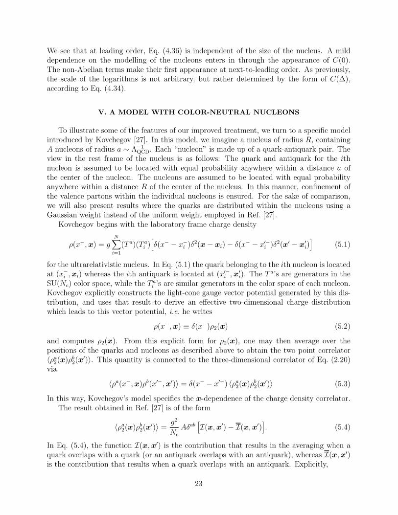
We see that at leading order, Eq. (4.36) is independent of the size of the nucleus. A milddependence on the modelling of the nucleons enters in through the appearance of C(0).The non-Abelian terms make their first appearance at next-to-leading order. As previously,the scale of the logarithms is not arbitrary, but rather determined by the form of C(∆),according to Eq. (4.34).

V. A MODEL WITH COLOR-NEUTRAL NUCLEONS

To illustrate some of the features of our improved treatment, we turn to a specific modelintroduced by Kovchegov [27]. In this model, we imagine a nucleus of radius R, containingA nucleons of radius a ∼ Λ−1

QCD. Each “nucleon” is made up of a quark-antiquark pair. Theview in the rest frame of the nucleus is as follows: The quark and antiquark for the ithnucleon is assumed to be located with equal probability anywhere within a distance a ofthe center of the nucleon. The nucleons are assumed to be located with equal probabilityanywhere within a distance R of the center of the nucleus. In this manner, confinement ofthe valence partons within the individual nucleons is ensured. For the sake of comparison,we will also present results where the quarks are distributed within the nucleons using aGaussian weight instead of the uniform weight employed in Ref. [27].

Kovchegov begins with the laboratory frame charge density

ρ(x−,x) = gN∑

i=1

(T a)(T ai )

[δ(x− − x−i )δ

2(x− xi)− δ(x− − x′−i )δ2(x′ − x′i)]

(5.1)

for the ultrarelativistic nucleus. In Eq. (5.1) the quark belonging to the ith nucleon is locatedat (x−i ,xi) whereas the ith antiquark is located at (x′−i ,x

′i). The T

a’s are generators in theSU(Nc) color space, while the T a

i ’s are similar generators in the color space of each nucleon.Kovchegov explicitly constructs the light-cone gauge vector potential generated by this dis-tribution, and uses that result to derive an effective two-dimensional charge distributionwhich leads to this vector potential, i.e. he writes

ρ(x−,x) ≡ δ(x−)ρ2(x) (5.2)

and computes ρ2(x). From this explicit form for ρ2(x), one may then average over thepositions of the quarks and nucleons as described above to obtain the two point correlator〈ρa2(x)ρb2(x′)〉. This quantity is connected to the three-dimensional correlator of Eq. (2.20)via

〈ρa(x−,x)ρb(x′−,x′)〉 = δ(x− − x′−) 〈ρa2(x)ρb2(x′)〉 (5.3)

In this way, Kovchegov’s model specifies the x-dependence of the charge density correlator.The result obtained in Ref. [27] is of the form

〈ρa2(x)ρb2(x′)〉 = g2

NcAδab

[I(x,x′)− I(x,x′)

]. (5.4)

In Eq. (5.4), the function I(x,x′) is the contribution that results in the averaging when aquark overlaps with a quark (or an antiquark overlaps with an antiquark), whereas I(x,x′)is the contribution that results when a quark overlaps with an antiquark. Explicitly,

23

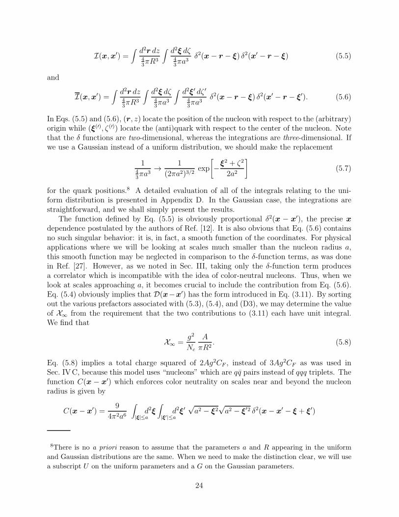
I(x,x′) =∫d2r dz43πR3

∫d2ξ dζ43πa3

δ2(x− r − ξ) δ2(x′ − r − ξ) (5.5)

and

I(x,x′) =∫d2r dz43πR3

∫d2ξ dζ43πa3

∫d2ξ′ dζ ′

43πa3

δ2(x− r − ξ) δ2(x′ − r − ξ′). (5.6)

In Eqs. (5.5) and (5.6), (r, z) locate the position of the nucleon with respect to the (arbitrary)origin while (ξ(′), ζ (′)) locate the (anti)quark with respect to the center of the nucleon. Notethat the δ functions are two-dimensional, whereas the integrations are three-dimensional. Ifwe use a Gaussian instead of a uniform distribution, we should make the replacement

143πa3

→ 1

(2πa2)3/2exp

[−ξ2 + ζ2

2a2

](5.7)

for the quark positions.8 A detailed evaluation of all of the integrals relating to the uni-form distribution is presented in Appendix D. In the Gaussian case, the integrations arestraightforward, and we shall simply present the results.

The function defined by Eq. (5.5) is obviously proportional δ2(x − x′), the precise x

dependence postulated by the authors of Ref. [12]. It is also obvious that Eq. (5.6) containsno such singular behavior: it is, in fact, a smooth function of the coordinates. For physicalapplications where we will be looking at scales much smaller than the nucleon radius a,this smooth function may be neglected in comparison to the δ-function terms, as was donein Ref. [27]. However, as we noted in Sec. III, taking only the δ-function term producesa correlator which is incompatible with the idea of color-neutral nucleons. Thus, when welook at scales approaching a, it becomes crucial to include the contribution from Eq. (5.6).Eq. (5.4) obviously implies that D(x−x′) has the form introduced in Eq. (3.11). By sortingout the various prefactors associated with (5.3), (5.4), and (D3), we may determine the valueof X∞ from the requirement that the two contributions to (3.11) each have unit integral.We find that

X∞ =g2

Nc

A

πR2. (5.8)

Eq. (5.8) implies a total charge squared of 2Ag2CF , instead of 3Ag2CF as was used inSec. IVC, because this model uses “nucleons” which are qq pairs instead of qqq triplets. Thefunction C(x − x′) which enforces color neutrality on scales near and beyond the nucleonradius is given by

C(x− x′) =9

4π2a6

∫

|ξ|≤ad2ξ

∫

|ξ′|≤ad2ξ′

√a2 − ξ2

√a2 − ξ′2 δ2(x− x′ − ξ + ξ′)

8There is no a priori reason to assume that the parameters a and R appearing in the uniform

and Gaussian distributions are the same. When we need to make the distinction clear, we will use

a subscript U on the uniform parameters and a G on the Gaussian parameters.

24

=9Θ(1−X)

16πa2

[(2 +X2)

√1−X2 −X2(4−X2) tanh−1

√1−X2

](5.9)

for a uniform distribution of quarks and nucleons and

C(x− x′) =e−X2

4πa2(5.10)

for the Gaussian distribution. In Eqs. (5.9) and (5.10) we have defined the dimensionlessdistance measure X ≡ |x−x′|/(2a) (for details, see Appendix D). These two functions havebeen plotted in Fig. 1. In the uniform case, C(x−x′) vanishes identically for |x−x′| ≥ 2a,whereas in the Gaussian case it has, not surprisingly, a Gaussian tail. Both functions arefinite at the origin.

Now that we have specified the functional form of D(∆), we may return to Eqs. (3.9)and (3.10) and evaluate the inputs to the correlation function, L(x−x′) and L(x−x′). Inthe uniform case we obtain

L(x− x′) =a2

4π

[(93

100+

373

200X2 − 491

800X4 − 1

64X6

)√1−X2

−(2

5+ 2X2 − 1

4X6 +

1

64X8

)tanh−1

√1−X2

]Θ(1−X)

− a2

20π

[93

20+ ln

(X2

4

)](5.11)

and

L(x− x′) =1−X2

32π

[(8 + 8X2 −X4) tanh−1

√1−X2 − (14 +X2)

√1−X2

]Θ(1−X).

(5.12)

The asymptotic forms of these functions are

L(x− x′) ∼

a2X2

4π

[ln(X2

4

)+

3

2

], X ≪ 1;

− a2

20π

[ln(X2

4

)+

93

20

], X ≫ 1;

(5.13)

and

L(x− x′) ∼

− 1

8π

[ln(X2

4

)+

7

2

], X ≪ 1;

0 (exactly), X ≫ 1.

(5.14)

Because L(x − x′) vanishes at large distances, the Fourier transform of the correlationfunction (2.21) constructed from (5.11) and (5.12) will remain finite at zero (transverse)momentum.

25

If instead we employ Gaussian distributions for the quarks we obtain

L(x− x′) =a2

4π

[(1 +X2) Ei(−X2) + exp(−X2)− ln(X2)− (1 + γE)

](5.15)

and

L(x− x′) = − 1

8πEi(−X2). (5.16)

Eqs. (5.15) and (5.16) contain the exponential integral function evaluated at negative valuesof the argument. We have employed the conventions of Ref. [32], i.e.

Ei(−z) ≡ −∫ ∞

x

dt

te−t, (z > 0). (5.17)

Also appearing in the first of these two equations is Euler’s constant γE . Asymptotically,we have

L(x− x′) ∼

a2X2

4π

[ln(X2) + γE − 2

], X ≪ 1;

− a2

4π

[ln(X2)− (1 + γE)

], X ≫ 1;

(5.18)

and

L(x− x′) ∼

− 1

8π

[ln(X2) + γE

], X ≪ 1;

1

8π

exp(−X2)

X2, X ≫ 1.

(5.19)

In this case, L(x − x′) has an exponential tail at large distances, and we end up with acorrelation function which falls like exp(−X2)/[X2 ln(X2)] in the infrared. Again, the gluonnumber density will be finite at zero transverse momentum.

We have compiled a series of plots (Figs. 2–6) to aid in the comparison of the twomodels to each other and to the results of Ref. [12]. Each version of the correlation functioneffectively depends on two parameters, which we take to be X∞ and aU , aG, or ΛQCD.In preparing these plots, we have adjusted these parameters so that the ultraviolet limitof (2.21) is identical for all three cases. Recall that in the ultraviolet limit, X∞ appearsmultiplicatively [see Eq. (2.24)]. Thus, matching in the ultraviolet really means matchingthe values of L at short distances. From (4.17), (5.14) and (5.19), we determine that

aG = 2 exp(γE2− 7

4

)aU

≈ 0.464aU (5.20)

and

ΛQCD = 14e7/4a−1

U

26

≈ 1.44a−1U . (5.21)

In Fig. (2), we have plotted the trace of the correlation function (2.21) in position spaceversus the dimensionless distance X . In drawing these curves, we have assumed that thelongitudinal coordinates have been fixed at some value such that a2χ(x−, x′−) = 20. Noticethat the curve for the MV correlator given in Eq. (2.30) begins to diverge significantly fromthe other two curves nearX = 0.3. At X ≈ 0.347, corresponding to |x−x′| = Λ−1

QCD, the MVcorrelator vanishes. Beyond this point, it rockets off to −∞ faster than any exponential. Incontrast, both the uniform and Gaussian curves are well-behaved. The correlation functiongenerated from the uniform quark/nucleon distribution vanishes for X ≥ 1.

Next, we perform the Fourier transform to form the gluon number density, Eq. (4.9).The results are plotted in Fig. (3) for a fixed value of the longitudinal momentum q+. Inorder to define the Fourier transform in the MV case, we have done what was suggested inRef. [19] and simply cut off the ∆ integration at Λ−1

QCD. All three curves have generally thesame over-all shape: a plateau at small values of q, a sharp decrease at intermediate valuesof q, and a tail for large values of q. The differing values for q → 0 may easily understoodfrom the position space functions in Fig. 2. The MV curve has the smallest number ofzero momentum gluons because of the abrupt cut-off imposed at ∆ = Λ−1

QCD. There aremore zero momentum gluons in the uniform case, since the corresponding position spacefunction extends out to |x−x′| = 2a. Finally, the exponential tail at large distances in theGaussian case produces even more zero momentum gluons. At large momenta, the gluonnumber density is supposed to go like 1/q2. To illustrate this transition, we have plottedthe gluon number density multiplied by (aq)2 in Fig. 4. In this figure, the uniform andGaussian curves are virtually indistinguishable. Beyond (aq)2 = 104, they remain flat. Theoscillations visible in the MV curve are a result of the sharp cutoff of the Fourier transformintegral. As (aq)2 grows, they become more rapid, but decrease in amplitude.

Next, we illustrate the effects of the non-Abelian contributions to the correlation function.For Fig. 5, we generate the ratio

〈Aai (x

−,x)Aai (x

′−,x′)〉all orders

〈Aai (x

−,x)Aai (x

′−,x′)〉lowest order

=eNcχL(x−x′) − 1

NcχL(x− x′). (5.22)

From this expression, we see that the relative importance of the non-Abelian terms dependson the magnitude of χ: if χ → 0, then this ratio goes to 1. Fig. 5 plots this ratio forvarious values of a2χ ranging from 2 to 40 using the uniform version of Kovchegov’s model.9

We see that the non-Abelian terms have the effect of suppressing the magnitude of thecorrelation functions at large distances relative to the Abelian result. In momentum space,this translates into a depletion of low momentum gluons.

Finally, we present Fig. 6. This is a plot of the all-orders gluon density (4.9) divided bythe lowest-order gluon density (4.17) at fixed q+ for various values of X∞. We see that forsmall values of q, there are fewer gluons as X∞ increases. At very large values of q, there

9If we employ Eq. (5.8) and set R ≈ A1/3a, we find that a typical magnitude for a2χ is approxi-

mately 2.5 for uranium.

27

is no change. On the other hand, at small values of q, this ratio is less than one, signallingthat in this region the number of gluons is no longer simply proportional to the number ofnucleons. The amount of suppression increases with increasing X∞, consistent with gluonrecombination scenario envisioned in Ref. [22]. Because of the transverse momentum sumrule (4.20), the area under each of the curves should be equal. Thus, we see a pile up ofgluons at intermediate values of q. These features of the gluon number density depend onlyon choosing a correlator consistent with color screening at large distances (sgnD(∆) = −1for large ∆).

We close this section by evaluating the parameters appearing in the expression for theaverage transverse momentum-squared within this model. According to Eq. (4.34), the valueof the scale associated with the momentum logarithms may be constructed from Eqs. (5.14)and (5.19):

Q0 =

12exp(−γE + 7

4) a−1

U ≈ 1.615a−1U , uniform distribution;

exp(−γE2) a−1

G ≈ 0.749a−1G , Gaussian distribution.

(5.23)

If we relate aU to aG in the manner specified by the ultraviolet matching condition (5.20),these two expressions become equal. On the other hand, the value of the smooth part of thecorrelation function at the origin appearing in Eq. (4.36) in the two models is

4πC(0) =

9

2a2U, uniform distribution;

1

a2G, Gaussian distribution.

(5.24)

These two quantities differ by a factor of 118exp(7

2− γE) ≈ 1.03 when Eq. (5.20) is applied.

In Figs. 7 and 8 we compare the approximate results for dN/dxF

and 〈q2〉 obtainedin Sec. IVD with “exact” curves generated by numerical integration of the full non-linearexpression for the gluon number density. Since Q0 does not depend on whether we use auniform or Gaussian distribution for the quarks, and C(0) only weakly so, we have employedthe uniform distribution in these plots, since its numerical integral is more convenient toset up. Fig. 7 is a plot of x

FdN/dx

Fdivided by the total charge-squared. In order to see

more easily how the next-to-leading order approximation (4.33) is performing, we have alsoplotted the ratio of the approximate to exact result in the region where the approximationbegins to diverge from the full all-orders value. We see that our approximation gives anexcellent description of the full result for (aQ)2 as low as about 10 when a2X∞ = 2. Ascould have been anticipated by studying Fig. 6, for a2X∞ = 40 our approximation begins tobreak down a bit sooner, at around (aQ2) = 50 or so.

Fig. 8 compares the exact and approximate curves for 〈q2〉 versus Q2. The cases X∞ = 2and X∞ = 40 differ by so little that they are virtually indistinguishable if presented on thesame plot. This is a consequence of the leading behavior 〈q2〉 ∝ Q2. For a2X∞ = 40 we haveshown the leading order approximation as well as the complete next-to-leading order curvegenerated from Eq. (4.36), since this value of X∞ is large enough for the difference betweenthe two approximations to be visible. We have also plotted the ratio of the approximateto exact results in the “interesting” region. The behavior of the a2X∞ = 40 result may

28

be understood in terms of Fig. 6: for large values of X∞, there is a pile-up of gluons atintermediate values of q2. This effect is purely non-Abelian in nature. Now, the leadingorder approximation is completely independent of any of the non-Abelian contributions tothe gluon number density. Thus, it is not surprising that the leading order expressionfalls short of the full result at moderate Q2. The first subleading contribution happens toovercorrect by a small amount (∼ 5%). Presumably the next term in the expansion will benegative in this region. In any event, the next-to-leading order expression is good to withina few percent for (aQ)2 as low as about 20 for both values of a2X∞.

VI. CONCLUSIONS

We have improved the McLerran-Venugopalan model by introducing a constraint on thecharge-density correlation function to ensure that it is consistent with a nucleus which is, asa whole, color neutral. We find that imposing color-neutrality eliminates the divergences inthe gluon number density present in the original MV model at small values of the transversemomentum, provided that the transverse part of the charge-density correlation function,D(∆) is rotationally invariant and falls off faster than 1/∆4 at large distances. In thissituation, the gluon number density approaches a constant value as q → 0. To obtaina gluon number density which goes as ln q2 at small transverse momenta, we must haveD(∆) fall off more slowly than 1/∆4. This is permissible only if we impose the additionalconstraint that D(∆) < 0 at large distances. Then we can use a D(∆) which falls off nearlyas slowly as 1/∆2.

Because we have an expression which is mathematically well-behaved, we are able todemonstrate that the gluon distribution function within the MV model is proportional to1/x

Fto all orders in the coupling constant, independent of the functional form of µ2(x−).

This conclusion hinges upon the choice of a purely local dependence on the longitudinaldistance in the charge-density correlator. The inclusion of quantum corrections [12–18] isexpected to change this situation.

We have derived a transverse sum rule, Eq. (4.20), for the gluon number density. Thissum rule indicates that the total number of gluons may be computed as if the theory werepurely Abelian: the only effect of the non-Abelian terms is to shift gluons from one valueof transverse momentum to another. As a consequence of this sum rule, we have shownthat the gluon structure function in a nucleus at large Q2 is simply given by A times theresult of the DGLAP equation for a single nucleon. We have shown that if we employ acharge density correlator which is consistent with charge screening at large distances, thenwe have saturation [22]: as the density of color charge X∞ is increased, the number of lowmomentum gluons grows more slowly than the number of nucleons.

We have also presented relatively simple expressions for dN/dxF[Eq. (4.33)] and the

mean transverse momentum-squared [Eq. (4.36)] as a function of Q, accurate to order 1/Q2

and Q0 respectively within this model. We are able to compute the scales of the logarithmsin terms of a single model-dependent function C(∆) which describes the manner in whichcharge neutrality is approached at scales near and beyond the nucleon size. Rather re-markably, the complicated non-linear structure of the full gluon distribution function maybe understood in terms of the Q2 expansion. That is, only the Abelian terms enter in

29

at leading order in this expansion, with the non-Abelian contributions making their firstappearance at next-to-leading order.

ACKNOWLEDGMENTS

This research is supported in part by the Natural Sciences and Engineering ResearchCouncil of Canada and the Fonds pour la Formation de Chercheurs et l’Aide a la Rechercheof Quebec. GM would like to thank Guy Moore numerous insightful discussions during thecourse of this work. CSL would like to thank Larry McLerran for instructive discussionsabout his model.

30

APPENDIX A: NOTATION AND CONVENTIONS

We begin by defining the light-cone coordinates x±:

x± ≡ x0 ± x3√2

. (A1)

The transverse coordinates x1 and x2 form a two-dimensional vector which we denote simplyas x, without the usual subscript “T” or “⊥” to avoid excessive clutter. Our metric has thesignature (−,+,+,+). Thus, the light-cone dot product reads qµxµ = −q+x−−q−x++q ·x,and x± = −x∓. We will think of x+ as the time coordinate, and x− as the longitudinaldistance coordinate (z).

Occasionally it will be helpful to switch to sum and difference coordinates. We willemploy the convention

Σ ≡ 12(x+ x′), ∆ ≡ x− x′. (A2)

This asymmetric pair of definitions has the desirable property of a unit Jacobian.The classical Yang-Mills equations are

DµFµν = Jν , (A3)

where we have employed matrix form, i.e. Jν ≡ T aJaν , etc. The T a are the normalizedHermitian generators of SU(Nc) in the fundamental representation, satisfying 2Tr(T aT b) =δab. The covariant derivative is

DµFµν ≡ ∂µF

µν − i[Aµ, F

µν]

(A4)

and the field strength is defined in terms of the potential as

F µν ≡ ∂µAν − ∂νAµ − i[Aµ, Aν

]. (A5)

These definitions assume that the coupling constant g has been absorbed into Jν [see, forexample, Eq. (5.1)]. Note that this is not the same convention as employed by MV inRefs. [1–4,12], where they choose to explicitly extract the factor of g from the current. Wedefine the charge density ρ(x−,x) appearing in Eq. (2.1) such that the total charge Z of thenucleus is given by

Z ≡∫dx−d2x ρ(x−,x). (A6)

Because our intuitive picture of the parton model is most simply realized in the light-conegauge [31], we elect to work primarily in that gauge. The light-cone gauge is defined by thecondition

A+(x) ≡ 0. (A7)

However, solution of the classical Yang-Mills equations for the type of source we consider issimplest in the covariant (Lorentz) gauge. For clarity, gauge-dependent quantities will bewritten with a tilde in the covariant gauge: e.g. A. The covariant gauge is specified by

∂µAµ(x) ≡ 0. (A8)

31

APPENDIX B: THE FUNCTION L(x− x′)

1. General Color-Neutral Correlator

In this appendix we present the calculation of L(x− x′) for a general correlator D(∆).Our starting point is Eq. (2.23) written in terms of the sum and difference variables definedas in (A2):

L(x− x′) ≡∫d2∆

∫d2Σ D(∆)

[G(x−Σ− 1

2∆)G(x′ −Σ+ 1

2∆)

− 12G(x−Σ− 1

2∆)G(x−Σ + 1

2∆)

− 12G(x′ −Σ− 1

2∆)G(x′ −Σ+ 1

2∆)

], (B1)

All three terms of (B1) may be evaluated by considering the integral

S(x,x′,∆) ≡ 1

16π2

∫d2Σ ln

( |x−Σ− 12∆|2

λ2

)ln( |x′ −Σ + 1

2∆|2

λ2

). (B2)

To deal with the logarithms, we insert the identity

ln(B

A

)=

∫ ∞

0

dz

z

(e−Az − e−Bz

). (B3)

Because we will ultimately insert our result for S into (B1), we may drop any terms whichdo not depend on ∆, thanks to the charge neutrality condition (3.7). Thus, the λ-dependentbits of (B2) do not contribute, and we are left with

S(x,x′,∆) =1

16π2

∫ ∞

0

da

a

∫ ∞

0

db

b

∫d2Σ exp

[−a(Σ− x+ 1

2∆)2 − b(Σ− x′ − 1

2∆)2

]. (B4)

The Σ integration is now Gaussian, and easily performed, yielding

S(x,x′,∆) =1

16π

∫ ∞

0

da

a

∫ ∞

0

db

b

1

a + bexp

− a(x− 1

2∆)2 − b(x′ + 1

2∆)2

+[a(x− 1

2∆) + b(x′ + 1

2∆)]2

a+ b

. (B5)

The next step is to insert

1 =∫ ∞

0

dτ

τδ(1− a+ b

τ

)(B6)

and rescale a→ τa, b→ τb. This allows us to simplify the exponent, producing

S(x,x′,∆) =1

16π

∫ ∞

0

dτ

τ 2

∫ ∞

0

da

a

∫ ∞

0

db

bδ(1− a− b) exp

−τa(1 − a)(x− x′ −∆)2

. (B7)

The b integration is now trivial, and the a integration becomes trivial after the variablechange

32

τ =u

a(1− a). (B8)

Thus, we obtain

S(x,x′,∆) =1

16π

∫ ∞

0

du

u2exp

−u(x− x′ −∆)2

, (B9)

which, when inserted into (B1) yields

L(x− x′) =1

16π

∫ ∞

0

du

u2

∫d2∆ D(∆)

[e−u(x−x′−∆)2 − e−u∆2

]. (B10)

Although the u integration in (B10) appears to be divergent, for a rotationally invariantcorrelation function D, the integral actually is finite. To see this, note that for small u theintegrand of (B10) looks like

du

u

[2(x− x′) ·∆− (x− x′)2

]D(∆) + finite terms. (B11)

The term containing (x−x′)2 vanishes when we perform the ∆ integration, because of (3.7).If D is rotationally invariant, then the angular part of the ∆ integration will cause the(x− x′) ·∆ term to vanish as well.

Because the integral over u is finite, we may employ a trick reminiscent of dimensionalregulation and write

L(x− x′) =1

16π

∫d2∆

∫ ∞

0

du

u2−ǫD(∆)

[e−u(x−x′−∆)2 − e−u∆2

], (B12)

where we understand that the limit ǫ→ 0 is to be taken on the right hand side as soon as itis safe to do so. The u integration may be performed by using the analytic continuation of

∫ ∞

0

du

uκ+1[e−βu − e−αu] =

1

κΓ(1− κ)[ακ − βκ] (B13)

(Eq. (3.434.1) of Ref. [32]). After applying (B13) to (B12) and performing some algebra weobtain

L(x− x′) =1

16π

1

ǫ

Γ(1− ǫ)

1− ǫ

∫d2∆D(∆)

[2∆ · (x− x′)− (x− x′)2

]

+1

16π

∫d2∆ D(∆)

[(x− x′ −∆)2 ln(x− x′ −∆)2 −∆2 ln∆2

](B14)

The pole term is the manifestation of the behavior described in (B11). For a rotationallyinvariant function D(∆), it vanishes. Thus, we are left with just

L(x− x′) =1

16π

∫d2∆ D(∆)

[(x− x′ −∆)2 ln(x− x′ −∆)2 −∆2 ln∆2

]. (B15)

Differentiation of (B15) to obtain explicit expressions for the two functions defined inEq. (2.25) produces

33

L(x− x′) =−1

8π

∫d2∆ D(∆) ln(x− x′ −∆)2 (B16)

and

Lij(x− x′) =−1

4π

∫d2∆ D(∆)

(x− x′ −∆)i(x− x′ −∆)j(x− x′ −∆)2

. (B17)

Recall that Lij was defined to be the traceless piece of ∂i∂′jL(x−x′). It does not contribute

to the gluon number density.

2. Rotationally Invariant Correlator

If D(∆) is rotationally invariant, we may perform the angular integration appearing inEq. (B15). Letting ψ be the angle between x and ∆ we have

L(x) =1

16π

∫ ∞

0d∆ ∆D(∆)

×∫ 2π

0dψ

[(x2 − 2x∆cosψ +∆2) ln(x2 − 2x∆cosψ +∆2)−∆2 ln∆2

](B18)

The non-trivial angular integrals appearing in this expression are

∫ 2π

0dψ ln(x2 − 2x∆cosψ +∆2) =

2π ln x2 if x > ∆;2π ln∆2 if x < ∆,

(B19)

and∫ 2π

0dψ cosψ ln(x2 − 2x∆cosψ +∆2) =

−2π∆/x if x > ∆;−2πx/∆ if x < ∆.

(B20)

Eqs. (B19) and (B20) force us to split up the radial integration into two pieces:

L(x) =1

8

∫ x

0d∆ ∆D(∆)

[(x2 +∆2) ln x2 −∆2 ln∆2 + 2∆2

]

+x2

8

∫ ∞

xd∆ ∆D(∆)

[ln∆2 + 2

]. (B21)

Similarly, we may perform the angular integration appearing in (B16) to obtain

L(x) = −1

4

∫ x

0d∆ ∆D(∆) ln x2 − 1

4

∫ ∞

xd∆ ∆D(∆) ln∆2. (B22)

Let us further assume that D(∆) = δ2(∆) − C(∆), where C(∆) is smooth at the origin.The color-neutrality requirement implies that

∫d2∆C(∆) = 1, or

∫ ∞

0d∆∆C(∆) =

1

2π. (B23)

Making this ansatz allows us to rewrite Eqs. (B21) and (B22) as

34

L(x) = − 1

8πx2 +

1

16πx2 ln

(x2

Ξ2

)+

1

8

∫ x

0d∆∆C(∆)

[(x2 +∆2) ln

(∆2

x2

)+ 2(x2 −∆2)

]

(B24)

and

L(x) = − 1

8πln(x2

Ξ2

)+

1

4

∫ x

0d∆∆C(∆) ln

(x2

∆2

), (B25)

where

ln Ξ2 ≡ 2π∫ ∞

0d∆∆C(∆) ln∆2. (B26)

Because of Eq. (B23), the integral defining the length scale Ξ in Eq. (B26) will be finitefor any reasonable function C(∆). Furthermore, the value of Ξ will be closely tied tothe scale implicit in C(∆), namely the nucleon size a ∼ Λ−1

QCD. Since we have stipulatedthat C(∆) be smooth at ∆ = 0, we conclude that Eqs. (B24) and (B25) are telling usthat L(x) and L(x) may be recast in the form of a power series in x plus lnx2 times apower series in x. Furthermore, the power series for L(x) begins at x0, whereas the firstnon-vanishing contribution to the series for L(x) is x2. This observation will be useful inorganizing the computation of the mean transverse momentum-squared associated with ourgluon distribution.

APPENDIX C: COMPUTATION OF THE AVERAGE TRANSVERSE

MOMENTUM-SQUARED

In this appendix we will outline the computation of the value of 〈q2〉, the average trans-verse momentum-squared for the gluon distribution (4.9). By definition

〈q2〉 ≡

∫

|q|≤Qd2q q2 dN

dxFd2q

∫

|q|≤Qd2q

dN

dxFd2q

. (C1)

We will do our computation through next-to-leading order. Since the numerator of (C1)grows like Q2 in the limit Q → ∞, this means we work to order Q0. Likewise, since thedenominator of (C1) grows like lnQ2 for large Q, we determine it through order 1/Q2.

For the purposes of this calculation we will assume that D(∆) is of the form

D(∆) = δ2(∆)− C(∆), (C2)

where the function C(∆) is smooth at the origin. As discussed in Sec. IVA, D(∆) shouldcontain δ2(∆) if the results are to agree with an Abelian theory in the ultraviolet. This isconsistent with having point-like quarks in the nucleons. Beyond specifying that C(∆) isrotationally invariant and has unit integral [to satisfy (3.7)], we will not make any additionalassumptions about this function.

35

1. Calculation of 〈q2〉dN/dxF

to Order Q0

We begin with the numerator of (C1), employing Eq. (4.8) for the integrand, since it hasa simpler transverse structure than Eq. (4.9). Thus, our starting point is

〈q2〉 dNdx

F

=N2

c − 1

2π3πR2 1

xF

∫ ∞

−∞dx−µ2(x−)

∫d2x

∫

|q|≤Qd2q q2eiq·xL(x)eNcX (x−)L(x). (C3)

If we were to evaluate the q integral as it stands, we would obtain a mildly complicatedcombination of Bessel and Lommel functions. Alternatively, we may replace q2eiq·x by−∇

2eiq·x. Then, the momentum integration appearing in (C3) is easily performed with thehelp of Ref. [32]:

∫

|q|≤Qd2q eiq·x = 2πQ2 J1(Qx)

Qx. (C4)

Observe that if the q integration were to extend to infinity instead of being cut off at Q,then the integral appearing in Eq. (C4) would have produced a delta function instead of aBessel function. Hence, we conclude that

limQ→∞

Q2 J1(Qx)

Qx= 2πδ2(x). (C5)

Eq. (C5) will serve as a useful diagnostic tool in determining the order in Q of each contribu-tion as it is encountered. That is, if the application of Eq. (C5) to a given expression resultsin a finite result, we will conclude that there are no contributions to that expression whichgrow as Q → ∞. On the other hand, if the result of applying Eq. (C5) is divergent, thenwe will have to do the integral involving the Bessel function exactly for finite Q, ensuringthat we correctly determine not only the contributions which grow as Q→ ∞, but also thesubleading terms as well.

After inserting (C4) into (C3), we integrate by parts to shift ∇2 off of the Bessel function.Thus, we arrive at

〈q2〉 dNdx

F

= −N2c − 1

π2πR2 1

xF

Q2∫ ∞

−∞dx−µ2(x−)

∫d2x

J1(Qx)

Qx∇

2[L(x)eNcX (x−)L(x)

]. (C6)

The derivatives appearing in Eq. (C6) yield

∇2[L(x)eNcX (x−)L(x)

]=

[∇

2L(x)]

+NcX (x−)L(x)[∇

2L(x)]

+2NcX (x−)[∂iL(x)

][∂iL(x)

]

+N2cX 2(x−)L(x)

[∂iL(x)

]2eNcX (x−)L(x). (C7)

The next steps are straightforward but tedious. Basically we have to examine each term bit-by-bit and do the x integration either after applying Eq. (C5) (for the constant contributions)

36

or by doing the actual integral with the Bessel function intact (for the contributions thatgrow as Q → ∞). Rather than go through all of this mathematics in detail, let us onlymention the highlights.

The first term in Eq. (C7), up to the ubiquitous exponential factor, is purely Abelian inorigin. Differentiation of Eq. (3.10) tells us that

∇2L(x) = −1

2D(x). (C8)

Thus, the contribution from this term is especially easy to compute, as there is no ∆

integration. The singular part of D(x) leads to a contribution proportional to Q2, whereasthe smooth part produces a constant piece proportional to C(0).

The second and third terms of (C7) are purely non-Abelian in origin. At lowest order(i.e. with the exponential set to unity), they are quadratic in the charge-squared. At theend of the day, the longitudinal dependence of these terms reads

∫ ∞

−∞dx−µ2(x−)X (x−) =

∫ ∞

−∞dx−

∫ x−

−∞dξ−µ2(x−)µ2(ξ−)

=1

2X 2

∞. (C9)

Thus, we see the result will be independent of the functional form of µ2(x−), as would havebeen manifest from the beginning had we chosen to begin our calculation with Eq. (4.9)instead of Eq. (4.8).

Because ∇2L(x) = −2L(x), the second term of (C7) contains L2(x). As a consequence,we encounter the transverse integrals

T1 ≡∫d2x

J1(Qx)

Qxln2 x2 (C10)

and

T2 ≡∫d2x

J1(Qx)

Qxlnx2 ln(x−∆)2. (C11)

The first of these two integrals reduces to

T1 =8π

Q

∫ ∞

0dxJ1(Qx) ln

2 x. (C12)

This integral may be evaluated by observing that Eq. (6.561.14) of Ref. [32] yields theidentity

∫ ∞

0dxJ1(Qx)x

ε =1

Q

(Q

2

)−εΓ(1 + ε/2)

Γ(1− ε/2). (C13)

Because ε is arbitrary, we may expand both sides of Eq. (C13) and equate correspondingpowers of ε to read off the integral of J1(Qx) times a logarithm to an arbitrary positiveinteger power. In the case of immediate interest we have

37

T1 =2π

Q2

[ln(Q2

4

)+ 2γE

]2. (C14)

We deal with T2 by first writing

T2 = 2∫d2x

J1(Qx)

Qx

[ln(Qx)− lnQ

]ln(x−∆)2. (C15)

Next, we rescale x ≡ y/Q in the first term to arrive at a form which possesses a transparentQ→ ∞ limit:

T2 = 2∫d2y

J1(y)

yln y ln

(y

Q−∆

)2

− lnQ2∫d2x

J1(Qx)

Qxln(x−∆)2. (C16)

In the first term of (C16), we may neglect y/Q in the logarithm and do the remainingintegral with the aid of Eq. (6.772.2) of Ref. [32]. In the second term we simply apply (C5).The result reads

T2 = −2π

Q2

[ln(Q2

4

)+ 2γE

]ln∆2. (C17)

The third term of Eq. (C7) contains among its contributions only one new non-trivialtransverse integral:

T3 ≡∫d2x

J1(Qx)

Qx

x ·∆x2

ln(x−∆)2. (C18)

We obtain the large-Q limit of (C18) by rescaling x ≡ y/Q and writing

ln(∆− y

Q

)2

= ln∆2 − 2y ·∆Q∆2

+O(

1

Q2

). (C19)

Then, (C18) becomes

T3 =1

Qln∆2

∫d2y

J1(y)

y

y ·∆y2

− 2

Q2

∫d2y

J1(y)

y

(y ·∆)2

y2. (C20)

The first term of (C20) posseses a vanishing angular integral, while the second term isstraightforward to evaluate. Thus,

T3 = −2π

Q2. (C21)

Finally, we remark that the fourth term of Eq. (C7), which consists of contributionswhich are cubic and higher in the charge density squared vanishes in the large-Q limit.

38

Essentially, this comes about because the small-x behavior of ∂iL(x) is xi[1 + lnx2]. Thus,the factor [∂iL(x)]

2 contains sufficient powers of x in this region to kill off the diverginglogarithms.

After working through all of the necessary algebra, we arrive at the surprisingly simpleresult

〈q2〉 dNdx

F

=1

xF

Z2

4π2

[Q2 − 4πC(0)

]

+1

xF

Z2

4π2

NcX∞

8π

[ln(Q2

4

)+ 2γE +

∫d2∆C(∆) ln∆2

]2

− 2

[ln(Q2

4

)+ 2γE +

∫d2∆C(∆) ln∆2

]− 2

, (C22)

where we have denoted the total charge-squared of the nucleus (N2c −1)X∞πR

2 by Z2. Eachoccurence of lnQ2 in Eq. (C22) comes with the same combination of γE and integral overC(∆), leading to the definition of Q0 presented in Eq. (4.34).

2. Calculation of dN/dxF

to Order 1/Q2

We now turn to the denominator of (C1). Previously, we presented Eq. (4.24), whichwrites this quantity in terms of the momentum space representation of the charge densitycorrelation function D(q). However, since the numerator has been expressed in terms of theposition space function C(∆), it will be useful to do the same for the denominator as well.Besides, Eq. (4.24) is correct only to leading order, and we require the 1/Q2 terms as well.

To obtain such an expression, we again employ Eq. (4.8) for the integrand:

dN

dxF

=N2

c − 1

2π3πR2 1

xF

∫ ∞

−∞dx−µ2(x−)

∫d2x

∫

|q|≤Qd2q eiq·xL(x)eNcX (x−)L(x). (C23)

The momentum integration appearing in (C23) may be done by applying Eq. (C4), producing

dN

dxF

=N2

c − 1

π2πR2 1

xF

Q2∫ ∞

−∞dx−µ2(x−)

∫d2x

J1(Qx)

QxL(x)eNcX (x−)L(x). (C24)

Since we are working to order 1/Q2, it is not enough to simply apply Eq. (C5) to replace theBessel function by a delta function when it is safe to do so, since this would make order 1/Q2

errors. Instead we will have to expand the exponential and apply an assortment of scalingarguments to determine the order of each contribution. We will denote the contribution todN/dx

Fwhich contains m powers of NcX (x−)L(x) by dN (m)/dx

F.

At zeroth order in this expansion we have

dN (0)

dxF

= − Z2

8π3

1

xF

Q2

∫d2x

J1(Qx)

Qxlnx2 −

∫d2∆C(∆)

∫d2x

J1(Qx)

Qxln(x−∆)2

.

(C25)

39

where we have used Eqs. (3.10) and (C2) to write out L(x). The x-integration in the firstterm of (C25) may be performed exactly with the aid of Eq. (6.772.2) of Ref. [32]:

∫d2x

J1(Qx)

Qxlnx2 = −2π

Q2

[ln(Q2

4

)+ 2γE

]. (C26)

The second term, which will combine with the logarithm in (C26) to make its argumentdimensionless, requires a bit more work. To this end we define

T4 ≡ Q2∫d2∆C(∆)

∫d2x

J1(Qx)

Qxln(x−∆)2. (C27)

The rescaling x ≡ w∆ produces

T4 = Q∫d2∆C(∆)∆ ln∆2

∫d2w

J1(wQ∆)

w

+ Q∫d2∆C(∆)∆

∫d2w

J1(wQ∆)

wln(w − ∆)2 (C28)

where ∆ is a unit vector in the ∆ direction. We may immediately perform the w integrationexactly in the first term of (C28). In the second term, we rescale, ∆ ≡ ∆′/(wQ):

T4 =∫d2∆C(∆) ln∆2

+1

Q2

∫d2w

∫d2∆′C

(∆′

wQ

)∆′J1(∆

′)1

w4ln(w − ∆)2. (C29)

The only angular dependence in the second term is contained in the logarithm. Thus,Eq. (B19) may be applied to yield

T4 =∫d2∆C(∆) ln∆2

+2π

Q2

∫ ∞

1

dw

w3lnw2

∫d2∆′C

(∆′

wQ

)∆′J1(∆

′). (C30)

Thanks to the theta-function from Eq. (B19), the radial part of the w integration begins atw = 1, not w = 0. If we now expand the correlation function in powers of ∆′/(wQ), thew integration will always converge. Likewise, we may always do the ∆′ integration via theanalytic continuation of Eq. (6.561.14) of Ref. [32]. Thus, we obtain a well-defined expansionof the second term of (C30) in powers of 1/Q. In particular, the 1/Q2 term vanishes, since

∫ ∞

0d∆∆2J1(∆) = 0. (C31)

Thus, only the first term of Eq. (C30) contributes through order 1/Q2. Combining thisresult with Eqs. (C25) and (C26) we arrive at

dN (0)

dxF

=1

xF

Z2

4π2

[ln(Q2

4

)+ 2γE +

∫d2∆C(∆) ln∆2

]. (C32)

40

The next term in the expansion of the exponential of Eq. (C24) will produce contributionsof order 1/Q2. Our overview of this part of the calculation begins with the result of doingthe expansion, which reads

dN (1)

dxF

≡ Z2

2π2NcX∞

1

q+Q2

∫d2x

J1(Qx)

QxL(x)L(x). (C33)

Eqs. (3.9) and (3.10) when combined with Eq. (C2) tell us that there are three kinds ofcontributions to Eq. (C33). The first is generated by multiplying the δ function containingterms of L(x) and L(x). It may be evaluated exactly with the help of

∫ ∞

0dxx2 ln2 xJ1(Qx) =

2

Q3

[ln(Q2

4

)+ 2γE − 1

], (C34)

which was obtained via the same methods used to integrate Eq. (C12).The second type of contribution to Eq. (C33) consists of terms produced by combining

a δ function from one factor [L(x) or L(x)] with the smooth part of the other. Generally,these contributions are handled in the same fashion as T4 [Eqs. (C27)–(C30)]. In particular,we extract the 1/Q2 terms via the rescaling x = w∆ followed by ∆ = ∆′/(wQ). The onlycomplication that arises is the appearance of the integral

T6 ≡ − Q

4π

∫d2∆C(∆)∆3

∫d2w

w · ∆w

J1(wQ∆) ln(w∆)2 ln(w − ∆)2. (C35)

The angular part of the w integration is governed by Eq. (B20), leading to

T6 =Q

2

∫d2∆C(∆)∆3

∫ ∞

0dwJ1(wQ∆) ln(w∆)2

[Θ(w − 1)− w2Θ(1− w)

]. (C36)

We may apply our usual rescaling of ∆ to the first term of (C36) to deduce that it is oforder (lnQ2)/Q4, and so may be neglected. However, in the second term, we cannot rescale∆ in this manner since the w integration would diverge. Instead, we write w ≡ v/(Q∆),yielding

T6 =1

2Q2

∫d2∆C(∆)

∫ Q∆

0dv v2(ln v2 − lnQ2)J1(v). (C37)

If we let the upper limit of the v integration go to infinity, we see that the integral remainsfinite. Therefore, we conclude that

T6 = − 2

Q2, (C38)

correct through order 1/Q2.The final type of contribution to (C33) which we encounter is generated by multiplying

the smooth parts of both factors, leading to the formidible-looking integral

∫d2x

J1(Qx)

Qx

∫d2∆C(∆)

[(x−∆)2 ln(x−∆2)−∆2 ln∆2

] ∫d2∆′C(∆′) ln(x−∆′)2.

(C39)

41

By employing the rescalings ∆ ≡ ∆x and ∆′ ≡ ∆′x followed by x ≡ y/Q, it is straightfor-

ward to show that the leading contribution to (C39) is of order (ln2Q2)/Q6.At the end of this lengthy procedure we arrive at

dN (1)

dxF

= − 1

xF

Z2

4π2

NcX∞

4πQ2

[ln(Q2

4

)+ 2γE +

∫d2∆C(∆) ln∆2

]. (C40)

When combined with Eq. (C32), we obtain the result (4.33) presented in Sec. IVD.

APPENDIX D: THE INTEGRALS APPEARING IN KOVCHEGOV’S MODEL

1. The Charge Density Correlation Function

In Sec. V, we wrote the charge density correlation function derived from Kovchegov’smodel [27] in terms of the two integrals I and I, given by Eqs. (5.5) and (5.6) respectively.In this Appendix, we will explicitly evaluate these expressions assuming that the nuclearradius R is much larger than the nucleon radius a.

The easier of the two integrals to evaluate is I. Because the nucleus and nucleons arespherical and we assume a sharp cut-off in the allowed positions of the nucleons and thequarks, we have

I(x,x′) =9

4

δ2(x− x′)

π2R3a3

∫

|ξ|≤ad2ξ

∫

|r|≤Rd2r

√R2 − r2

√a2 − ξ2 δ2(x− r − ξ). (D1)

Now an exact evaluation of (D1) would require that we satisfy the δ-function by settingr ≡ x − ξ and integrating over only those values of ξ which are compatible with this.However, since we take R ≫ a, we may approximate by setting r2 ≈ x2 in the integrandand performing the ξ integration over the entire disk of radius a. By doing this, we areallowing nucleons which are located near the edge of the nucleus to “pop out” by a (small)amount of order a. In this approximation, a straightforward evaluation yields

I(Σ,∆) =3

2πR2

√

1− Σ2

R2Θ(R2 −Σ2

)δ2(∆). (D2)

where we have switched to the sum and difference variables (A2). Now Eq. (D2) dependsuponΣ whereas the expressions employed in Sec. V do not. The Σ-dependence of Eq. (D2) isnot really surprising, since the pancake obtained by Lorentz-contracting a spherical nucleusshould be thinner near the edges than near the center. What we call X∞ in Eq. (5.8) isobtained from (D2) by first integrating over Σ: i.e. instead of simply writing πR2 for the Σintegral, as was done in the discussion following Eq. (4.1), we perform that integral includingthe geometric factors indicated in (D2):

∫d2Σ I(Σ,∆) = δ2(∆). (D3)

Comparing this result with Eqs. (5.3) and (5.4), we conclude that

42

πR2X∞ =g2N

Nc

. (D4)

The other integral is somewhat more difficult to evaluate. Doing the longitudinal inte-grations and making the R ≫ a approximation described above yields

I(Σ,∆) =27

π3R2a6

√

1− Σ2

R2Θ(R2 −Σ2)

×∫

|ξ|≤ad2ξ

∫

|ξ′|≤ad2ξ′

√a2 − ξ2

√a2 − ξ′2 δ2(∆− ξ + ξ′)

≡ 3

2πR2

√

1− Σ2

R2Θ(R2 −Σ2)C(∆) (D5)

where C is the function introduced in Eq. (5.9). Since we have defined C(∆) by extractingthe same Σ-dependent prefactor which appeared in (D2), at the end of the day we find thatD(∆) = δ2(∆)− C(∆), as written in Eq. (3.11).

A direct evaluation of the integral defining C is difficult because of the δ-function con-straint: we are instructed to consider the area of overlap between two disks of radius aseparated by a distance ∆. This area must be weighted by the product of the distances fromthe two centers to the integration point (see Fig. 9). Although this sounds simple, the onlyimmediate conclusion which may be drawn directly from the integral is that when |∆| ≥ 2athe function vanishes: the disks do not overlap.

To deal with the situation when |∆| ≤ 2a, we begin by computing the Fourier transformof C(∆):

C(q) ≡∫d2∆ e iq·∆ C(∆)

=9

4π2a6

∫

|ξ|≤ad2ξ

∫

|ξ′|≤ad2ξ′

∫d2∆ e iq·∆

√a2 − ξ2

√a2 − ξ′2 δ2(∆− ξ + ξ′) (D6)

Since the ∆ integration is over all space, the δ-function constraint can be satisfied for allvalues of ξ and ξ′: no messy Θ-functions are introduced. In fact, the entire expressionfactorizes:

C(q) =

3

2πa3

∫

|ξ|≤ad2ξ eiq·ξ

√a2 − ξ2

2

. (D7)

Performing the angular integration and rescaling the radial integral to unit range we obtain

C(q) =

3∫ 1

0dv v

√1− v2 J0(aqv)

2

. (D8)

The radial integral may be performed with the help of Ref. [32] (c.f. Eq. (6.567.1)):

C(q) =

3

√π

2

J3/2(aq)

(aq)3/2

2

. (D9)

43

Happily, the half-integer Bessel functions are expressible as trigonometric polynomials.Thus, we arrive finally at

C(q) =9

(aq)6

[sin(aq)− (aq) cos(aq)

]2. (D10)

In spite of the apparent high-order singularity at q = 0, C(0) is nevertheless finite:

limq→0

C(q) = 1. (D11)

It is amusing to note that the function implied by (D11) for the Fourier transform of D,namely

D(q) = 1− 9

(aq)6


]2. (D12)

is exactly the same function that arises in position space for the parallel spin pair correlationfunction in a noninteracting gas of spin-1

2fermions [33]. In the Fermi gas, the role of the

sphere of radius a containing a uniform distribution of quarks is played by the momentum-space filling of energy levels up to the Fermi surface. The condition that the nucleons becolor neutral on large scales leads to the vanishing of D at zero momentum. The Pauliexclusion principle leads to the vanishing of the parallel spin pair correlation function atzero separation.10

Returning to the issue at hand, to obtain C(∆), we simply invert the Fourier transform.The angular integration is straightforward, and leaves us with

C(∆) =9

4πa2

∫ ∞

0dq J0

(q∆

a

)[1

q3+

1

q5+

cos 2q

q3− 2 sin 2q

q4− cos 2q

q5

]. (D13)

Each of the five terms on the right-hand-side of (D13) is individually divergent. In order toperform the q integration term-by-term, we must insert a regulator. Since the final combi-nation of terms in (D13) is guaranteed to be finite by (D11), the result will be insensitiveto the details of the regulator employed. A convenient means of regulation is to make thereplacement

J0

(q∆

a

)→ J2ǫ

(q∆

a

)(D14)

in (D13). We may then apply Eqs. (6.561.14), (6.699.1), and (6.699.2) of Ref. [32] to obtain

C(∆) =9

4πa2

−X

2

2

1

ǫ

1

1− ǫ2+X4

8

1

ǫ

1

(1− ǫ2)(1− ǫ2/4)

10The opposite spin pair correlation function for the Fermi gas is unity (the exclusion principle

does not affect particles of opposite spin). This case is analagous to the non-charge conserving

correlator of Eq. (2.4).

44

−2(X2

4

)ǫ cosπǫ

ǫ(1− 2ǫ)(2− 2ǫ)(3− 2ǫ)(4− 2ǫ)

×[(3− 2ǫ)(4− 2ǫ) 2F1(−1 + ǫ,−1

2+ ǫ; 1 + 2ǫ;X2)

−4(4− 2ǫ) 2F1(−1 + ǫ,−32+ ǫ; 1 + 2ǫ;X2)

+4 2F1(−2 + ǫ,−32+ ǫ; 1 + 2ǫ;X2)

], (D15)

which is valid for ∆ ≤ 2a. In this expression we have defined the dimensionless distanceX ≡ ∆/(2a). The hypergeometric functions may be expanded, and all of the poles in ǫcancelled. The resulting series may then be converted back into a different (generalized)hypergeometric function. The result of this tedious algebra is

C(∆) =9

64πa2

[2X2(4−X2) ln

(X2

4

)+ 8 +X4 − X6

23F2(1, 1,

52; 3, 4;X2)

]. (D16)

Finally, we notice that all but one of the parameters in the hypergeometric functionappearing in (D16) are integers. Hence, we may eliminate this hypergeometric function bycombining Eqs. (7.512.12) and (9.111) of Ref. [32] to obtain

3F2(a, b, c; p, q; z) =Γ(p)Γ(q)

Γ(b)Γ(p− b)Γ(c)Γ(q − c)

×∫ 1

0dt

∫ 1

0du tb−1(1− t)p−b−1uc−1(1− u)q−c−1(1− tuz)−a. (D17)

The required integrations are all straightforward, yielding

3F2(1, 1,52; 3, 4; z) = −4

z

(1− 4

z

)[ln(z

4

)+ 2 tanh−1

√1− z

]

+2

z+

16

z3− 8

z2

(1 +

2

z

)√1− z (D18)

Inserting (D18) into (D16) at last gives us

C(∆) =9

16πa2

[(2 +X2)

√1−X2 −X2(4−X2) tanh−1

√1−X2

], (D19)

which is true for X ≤ 1.

2. Computation of L(x− x′)

We now turn to the evaluation of L(x − x′). This function may be determined bythe same procedure used to determine C(∆). Since Eq. (3.10) expresses L(x − x′) as theconvolution of D with a logarithm, we may use (3.11) and (D10) to immediately write

45

L(q) = 1

2q2

1− 9

(aq)6


]2. (D20)

Once again we encounter an expression with a fake pole at the origin: the q → 0 limit isactually

limq→0

L(q) = a2

10. (D21)

So, to invert the Fourier transform, we may employ the same trick as was used on Eq. (D13):after the angular integration we replace the Bessel function of order zero by one of order 2ǫand integrate term-by-term. After verifying that all of the poles in ǫ do indeed cancel, weare left with

L(x− x′) =1

64π

[−(1−X2)(8 + 8X2 −X4) ln

(X2

4

)

−1

6(1−X2)(169− 47X2 + 7X4)

+1

6− 9X8

644F3(1, 1,

52, 4; 3, 5, 5;X2)

]. (D22)

This expression is valid only for X ≤ 1. Eq. (D22) displays the precise form predicted forL(x − x′) at the end of Appendix B: it is a power series in X2 plus lnX2 times anotherseries in X2. No odd powers of X appear in this series since we employed a rotationallyinvariant correlation function depending upon the vector x−x′, as opposed to an arbitraryfunction of |x− x′|.

The hypergeometric function may be eliminated from (D22) by combining (D17) withEq. (7.512.12) of Ref. [32]:

4F3(a, b, c, d; p, q, r; z) =Γ(p)Γ(q)Γ(r)

Γ(b)Γ(p− b)Γ(c)Γ(q − c)Γ(d)Γ(r − d)

×∫ 1

0ds

∫ 1

0dt

∫ 1

0du sb−1(1− s)p−b−1tc−1(1− t)q−c−1

×ud−1(1− u)r−d−1(1− stuz)−a, (D23)

from which we learn that

4F3(1, 1,52, 4; 3, 5, 5; z) = −64

9z

(1− 9

z+

8

z3

)[ln(z

4

)+ 2 tanh−1

√1− z

]

−128

9z2

(1 +

13

z− 14

z2

)√1− z

+224

27z− 64

z2+

256

z3− 1792

9z4. (D24)

The result of inserting (D24) into (D22) is precisely (5.12) except for the step-function. ForX > 1, it is easy to combine the integral representation for L given in Eq. (3.10) with theintegral form of C from Eq. (5.9) to show that that L(x− x′) vanishes in this region.

46

3. Computation of L(x− x′)

Finally, we come to L(x − x′). We should like to begin with the Fourier transformfunction L(q). Note that (2.25) implies

q2 L(q) = 2L(q). (D25)

Unfortunately, this relation is not sufficient to determine L(q) uniquely: we may add anarbitrary multiple of δ2(q2) to L(q) without contradicting Eq. (D25). According to theintegral representation of L(x−x′), L(0) vanishes. Therefore, we could adjust this arbitraryterm so that this is true when we invert the Fourier transform. Operationally, we may simplyinvert the expression implied by (D25) using the same method we have used on the otherintegrals in this Appendix and drop the pole and constant terms. Although this procedurelacks the satisfying feeling that comes when one sees the poles cancel automatically, it doesproduce the correct result, as has been verified by a direct numerical evaluation of theintegral in (3.9). The bottom line is that for X ≤ 1 we find

L(x− x′) =a2

4π

[(X2 − X6

8+X8

128

)ln(X2

4

)

+3X2

2− 9X4

8+

5X6

24− 5X8

384

+9X10

128004F3(1, 1,

52, 4; 3, 6, 6;X2)

](D26)

whereas for X ≥ 1

L(x− x′) = − a2

20π

[93

20+ ln

(X2

4

)]. (D27)

This latter result may be obtained inserting the integral representation (5.9) of C into theintegral representation (3.9) of L. Using the identity (D23) to evaluate the hypergeometricfunction appearing in (D26) gives:

4F3(1, 1,52, 4; 3, 6, 6; z) = −20

9z

(5− 80

z+

640

z3+

128

z4

)[ln(z

4

)+ 2 tanh−1

√1− z

]

− 8

9z2

(25 +

982

z− 2984

z2− 1488

z3

)√1− z

+500

27z− 8000

27z2+

1600

z3− 6400

3z4− 3968

3z5(D28)

Eqs. (D26)–(D28) combine to reproduce the expression presented in Eq. (5.11).

47

REFERENCES

∗ Electronic address: [email protected]† Electronic address: [email protected][1] L. McLerran and R. Venugopalan, Phys. Rev. D49, 2233 (1994). [hep-ph/9309289][2] L. McLerran and R. Venugopalan, Phys. Rev. D49, 3352 (1994). [hep-ph/9311205][3] L. McLerran and R. Venugopalan, Phys. Rev. D50, 2225 (1994). [hep-ph/9402335][4] A. Ayala, J. Jalilian-Marian, L. McLerran, and R. Venugopalan, Phys. Rev. D52, 2935

(1995). [hep-ph/9501324][5] A. Mueller, Nucl. Phys. B307, 34 (1988).[6] A. Mueller, Nucl. Phys. B317, 573 (1989).[7] A. Mueller, Nucl. Phys. B335, 115 (1990).[8] A. Mueller, Eur. Phys. J. A1, 19 (1998). [hep-ph/9710531][9] Yu. Kovchegov and A. Mueller, Nucl. Phys. B529, 451 (1998). [hep-ph/9802440][10] A.H. Mueller, “Parton saturation at small x and in large nuclei,” hep-ph/9904404.[11] A. Ayala, J. Jalilian-Marian, L. McLerran, and R. Venugopalan, Phys. Rev. D53, 458

(1996). [hep-ph/9508302][12] J. Jalilian-Marian, A. Kovner, L. McLerran, and H. Weigert, Phys. Rev. D55, 5414

(1997). [hep-ph/9606337][13] J. Jalilian-Marian, A. Kovner, A. Leonidov, and H. Weigert, Nucl. Phys. B504, 415

(1997). [hep-ph/9701284][14] J. Jalilian-Marian, A. Kovner, A. Leonidov and H. Weigert, Phys. Rev. D59, 014014

(1999). [hep-ph/9706377][15] J. Jalilian-Marian, A. Kovner and H. Weigert, Phys. Rev. D59, 014015 (1999). [hep-

ph/9709432][16] J. Jalilian-Marian, A. Kovner, A. Leonidov and H. Weigert, Phys. Rev. D59, 034007

(1999); erratum Phys. Rev. D59, 099903 (1999). [hep-ph/9807462][17] J. Jalilian-Marian and X.-N. Wang, “Small x gluons in nuclei and hadrons,” hep-

ph/9902411.[18] A. Kovner and J. Guilherme Milhano, “Vector potential versus color charge density in

low-x evolution,” hep-ph/9904420.[19] L. McLerran and R. Venugopalan, Phys. Lett. B424, 15 (1998). [nucl-th/9705055][20] M. Gyulassy and L. McLerran, Phys. Rev. C56, 2219 (1997). [nucl-th/9704034][21] S.V. Molodtsov, A.M. Snigirev and G.M. Zinovjev, Phys. Lett. B443, 387 (1998). [hep-

ph/9804418][22] L.V. Gribov, E.M. Levin, and M.G. Ryskin, Phys. Rep. 100, 1 (1983).[23] L. McLerran, “Three lectures on the physics of small x and high gluon density,” hep-

ph/9903536.[24] R. Venugopalan, “Parton saturation, production, and equilibrium in high energy nuclear

collisions,” hep-ph/9907209.[25] L.N. Lipatov, Sov. J. Nucl. Phys. 20, 95 (1975); V.N. Gribov and L.N. Lipatov, Sov. J.

Nucl. Phys. 15, 438 (1972); Yu. Dokshitzer, Sov. Phys. JETP 46, 641 (1977).[26] G. Alterelli and G. Parisi, Nucl. Phys. B126, 298 (1977).[27] Yu. Kovchegov, Phys. Rev. D54, 5463 (1996). [hep-ph/9605446][28] G. Curci, W. Furmanski, R. Petronzio, Nucl. Phys. B175, 27 (1980).

48


















http://arxiv.org/abs/nucl-th/9705055

http://arxiv.org/abs/nucl-th/9704034







[29] J.C. Collins and D.E. Soper, Nucl. Phys. B194, 445 (1982).[30] S.J. Brodsky and G.P. Lepage in Perturbative Quantum Chromodynamics, edited by

A.H. Mueller (World Scientific, 1989).[31] A.H. Mueller in Frontiers in Particle Physics, Cargese 1994, edited by M. Levy, J. Il-

iopoulos, R. Gastmans, and J.–M. Gerard, NATO Advanced Study Institute Series B,Physics, Vol. 350, (Plenum Press, 1995).

[32] I.S. Gradshteyn and I.M. Ryzhik, Table of Integrals, Series, and Products (AcademicPress, Inc., 1980).

[33] See for example, G. Baym, Lectures on Quantum Mechanics (The Benjamin/CummingsPublishing Company, 1969), p. 429.

49

FIGURES

FIG. 1. The smooth part of the two-point charge density correlation function in Kovchegov’s

model [27], as given in Eqs. (5.9) (uniform quark/nucleon distribution) and (5.10) (Gaussian

quark/nucleon distribution). The nucleon size parameters a have been chosen according to

Eq. (5.20) so that resulting gluon number densities match in the ultraviolet limit. In the uni-

form case, C(∆) vanishes for ∆ > 2a. In the Gaussian case, there is a Gaussian tail in this

region.

50

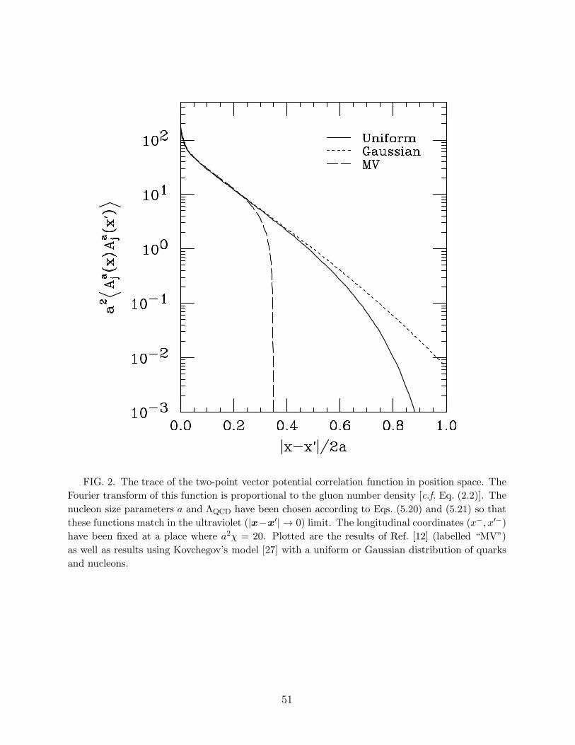
FIG. 2. The trace of the two-point vector potential correlation function in position space. The

Fourier transform of this function is proportional to the gluon number density [c.f. Eq. (2.2)]. The

nucleon size parameters a and ΛQCD have been chosen according to Eqs. (5.20) and (5.21) so that

these functions match in the ultraviolet (|x−x′| → 0) limit. The longitudinal coordinates (x−, x′−)

have been fixed at a place where a2χ = 20. Plotted are the results of Ref. [12] (labelled “MV”)

as well as results using Kovchegov’s model [27] with a uniform or Gaussian distribution of quarks

and nucleons.

51

FIG. 3. Plot of the gluon number density (4.9) at fixed q+. The nucleon size parameters a

and ΛQCD have been chosen according to Eqs. (5.20) and (5.21) so that these functions match in

the ultraviolet limit. The total charge squared per unit area has been set to a2X∞ = 20. Plotted

are the results of Ref. [12] (labelled “MV”) as well as results using Kovchegov’s model [27] with a

uniform or Gaussian distribution of quarks and nucleons.

52

FIG. 4. Plot of (aq)2 times the gluon number density (4.9) at fixed q+. This combination has

been chosen to enhance the high momentum part of the distribution and show the approach to the

predicted 1/q2 ultraviolet behavior. The nucleon size parameters a and ΛQCD have been chosen

according to Eqs. (5.20) and (5.21) so that these functions match in this limit. The total charge

squared per unit area has been set to a2X∞ = 20. Plotted are the results of Ref. [12] (labelled

“MV”) as well as results using Kovchegov’s model [27] with a uniform or Gaussian distribution of

quarks and nucleons.

53

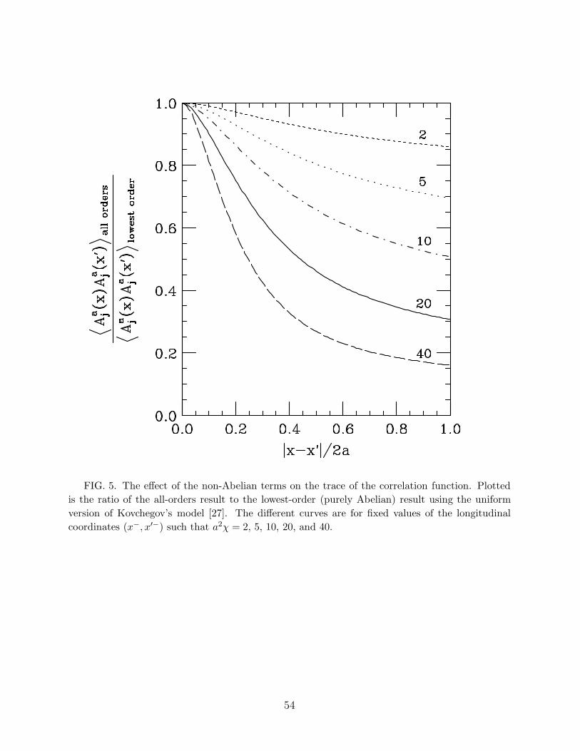
FIG. 5. The effect of the non-Abelian terms on the trace of the correlation function. Plotted

is the ratio of the all-orders result to the lowest-order (purely Abelian) result using the uniform

version of Kovchegov’s model [27]. The different curves are for fixed values of the longitudinal

coordinates (x−, x′−) such that a2χ = 2, 5, 10, 20, and 40.

54

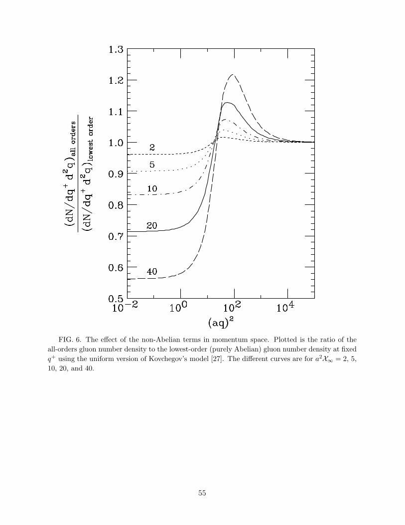
FIG. 6. The effect of the non-Abelian terms in momentum space. Plotted is the ratio of the

all-orders gluon number density to the lowest-order (purely Abelian) gluon number density at fixed

q+ using the uniform version of Kovchegov’s model [27]. The different curves are for a2X∞ = 2, 5,

10, 20, and 40.

55

FIG. 7. Top: Gluon structure function xFg(x

F, Q2) = x

FdN/dx

Fdivided by the total color

charge-squared for a large nucleus. Plotted is a comparison of the next-to-leading order approx-

imation (4.33) with the exact result obtained by numerical integration of (4.22) for two different

values of X∞. Bottom: The ratio of the next-to-leading order approximation to the exact result in

the region where the approximation begins to break down.

56

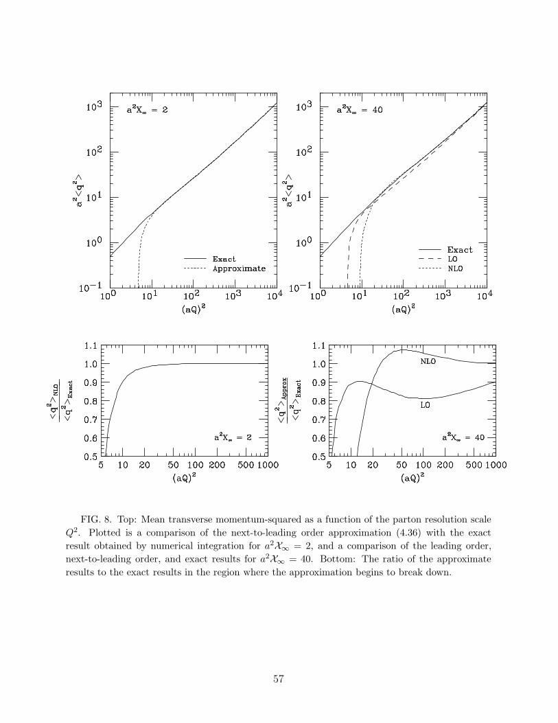
FIG. 8. Top: Mean transverse momentum-squared as a function of the parton resolution scale

Q2. Plotted is a comparison of the next-to-leading order approximation (4.36) with the exact

result obtained by numerical integration for a2X∞ = 2, and a comparison of the leading order,

next-to-leading order, and exact results for a2X∞ = 40. Bottom: The ratio of the approximate

results to the exact results in the region where the approximation begins to break down.

57

∆

ξ ξ’

aa

FIG. 9. The integration region encountered in Eq. (D5) for the smooth part of the correlation

function in the uniform version of Kovchegov’s model [27].

58

Documents

Color Neutrality and the Gluon Distribution in a Very ... · In Sec. III we describe the conditions which the charge-density correlator must satisfy in order to be consistent with