Color Measurement and Color Theory: I - Deep Blue

JOURNAL OF MATHEMATICAL PSYCHOLOGY 12, 283-303 (1975)

Color Measurement and Color Theory:

I. Representation Theorem for Grassmann Structures

DAVID H. KRANTZ

Department of Psychology, University of Michigan, 330 Packard Road, Ann Arbor, Michigan 48104

For trichromatic color measurement, the empirically based structure consists of the set of colored lights, with its operations of additive mixture and scalar multiplication, and the binary relation of metameric matching. The representing numerical structure is a vector space. The important axioms are Grassmann’s laws. The vector representation is constructed in a canonical or coordinate-free manner, mainly using Grassmann’s additivity law. Trichromacy is used only to fix the dimensionality.

Color theories attempt to get a more unique homomorphism by enriching the basic empirical structure with new empirical relations, subject to new axioms. Examples of such enriching relations include: discriminability or dissimilarity ordering of color pairs; dichromatic matching relations; and unidimensional matching relations, or codes. Representation theorems for the latter two examples are based on Grassmann-type laws also. The relationship between a Grassmann structure and its unidimensional Grassmann codes is modeled by the relationship between a vector space and its dual space of linear functionals. Dual spaces are used to clarify theorems relating to the three-pigment hypothesis and to reduction dichromacy.

This paper presents a new exposition of the foundations of trichromatic color measurement. There are three closely interrelated reasons that mandate a reexposition of this material. First, both the language of mathematics and the standards of mathematical rigor have progressed greatly in the past century. The subject of color measurement can be communicated more clearly to new generations of students if it is cast in modern mathematical concepts. Second, many points that are obscure or difficult in traditional treatments are much clearer if a slightly more abstract standpoint is assumed. Many modern ideas in linear algebra-especially the concept of linear functional and the resulting distinction between a linear space and its dual space-seem to be specially designed to clarify thinking about color theory. Much wasted time and many blind alleys can be avoided if strings of equations are replaced by simple abstract arguments. Thirdly, one obtains a new perspective on the interrelation between color

This paper extensively revises a 1971 technical report with the same title that was supported by NSF Grants GB 4947 and 8181. Preparation of this manuscript was supported by NSF GB 36642X.

283 Copyright 0 1975 by Academic Press, Inc. All rights of reproduction in any form reserved.

284 DAVID H. KRANTZ

measurement and color theories. This makes it much easier to survey the plethora of starting points for various extant color systems or theories, and to formulate more clearly some of the main unsolved empirical problems in color perception. This third point is reinforced by the second paper in this series (Krantz, 1975) which contains a new analysis of the foundations of opponent-colors theory, and by the first experimental fruits which stem from the latter analysis (Larimer, Krantz, and Cicerone, 1974, 1975).

The introduction shows how the representational viewpoint of measurement theory can be applied to color theory. The next two sections develop the classical vector representation based on Grassmann’s laws, but in a canonical fashion, rather than tied to specific coordinates. The final two sections present several results involving the relation of three-dimensional Grassmann structures to their one-dimensional and two-dimensional homomorphic images (codes and dichromatic reduction structures, respectively).

INTRODUCTION

In classical trichromatic color measurement any colored light u corresponds to a vector 4(u) with three real-valued components: 4(u) = (&(a), &(a), &(a)). The set A for which the function $ is defined consists of all possible spectral energy distributions of colored lights. This set of objects has two natural empirical operations: concatenation (a @ b is the light consisting of an additive mixture, or wavelength-by-wavelength energy sum, of lights a, b) and multiplication by positive scalars (t * a is the light obtained by changing the energy at each wavelength by the constant factor t). Those two operations involve only physics. The perception of color enters via the third empirical relation: metameric matching. Lights a, b are metameric (u - b) if they match in color. The numerical relations that correspond to 0, *, and - are, respectively, vector addition, multiplication of vectors by scalars, and equality. That is,

$Czez b) = $(a> + W, where + d eno t es ordinary vector addition; C(t * u) = t . $(a), . denotes multiplication by a scalar; and a - b if and only if 4(u) = $(b),

that is, a is metameric to b if and only if they have the same vector representation. In short, 4 is a homomorphism of the empirically based structure (A, 0, *, -) into the numerical (vector) structure (Re3, +, ., =).

Representation and Uniqueness Theorems

The homomorphism between empirical relations, such as (0, *, -) for color, and numerical relations in Re3, is a consequence of empirical laws satisfied by the empirical relations. The first goal of this paper is to state and prove the representation theorem and uniqueness theorem that establish the homomorphism 4 as a consequence of the empirical laws of color matching. The laws fall naturally into two classes: those

COLOR MEASUREMENT AND COLOR THEORY I 285

which involve only the physics of color mixture (0, *) and those which involve the relation N, based on perception. The latter group constitute a reformulation of Grassmann’s (1853-4) laws. The uniqueness theorem is the usual one for color measurement: any two representations are related by a nonsingular linear transformation. Instead of one arbitrary constant, the unit of measurement, there are nine free constants of a 3 X 3 matrix.

The Representational Viewpoint in Color Theory

Since the work of Helmholtz, most work in color theory has been concerned with discovering a special set of coordinates in color space, which would constitute the three “fundamental sensations” of color. Such special coordinates have been devised to attempt to fit various bodies of data. Hurvich and Jameson (1957) gave the first really comprehensive attempt to encompass all the major data on discrimination, perceptual attributes, color defects, and adaptation into a single theory. They used three coordinates corresponding to opponent processes.

These attempts to introduce special coordinates can be viewed a bit differently from the standpoint of representation and uniqueness theorems. From this standpoint, the goal of color theory is to enrich the relational structure (A, 0, *, -), by adding further perceptually based relations, and to extend the homomorphism 4 by finding simple numerical relations that correspond to or describe those added perceptual relations. The resulting representation theorem will be much stronger-its conclusion will impose many more assertions about the homomorphism +-and the uniqueness theorem will therefore restrict much more sharply the class of permissible homomorphisms. A sufficiently enriched empirical relational structure might yield a homomorphism that is unique (except for one or more choices of units of measurement).

To illustrate this idea, consider the problem of constructing a uniform color space. The added empirically based relation on A is one that contains information about the discriminability or similarity of colors. This can take the form of a quaternary relation: (a, b) 2 (a’, b’), meaning that the discriminability or the dissimilarity of a from b is at least as great as that of a’ from b’. It is not obvious what numerical relation in Re3 should correspond to this perceptual relation; the simplest possibility would be the ordering of Euclidean distances between the representing vectors +(a), 4(b). That is,

(a, b) 2 (a’, b’) if and only if +(a), 4(b)) 3 d($(a’), W)),

where 4$(a), W) is g iven by the Pythagorean formula

286 DAVID H. KRANTZ

Since ordering of Euclidean distances is not preserved by arbitrary nonsingular transformations, but only by orthogonal linear transformations and similarity transformations (changes of unit), the representing homomorphism $ (if one existed) would be unique only up to rotations and changes of unit. If instead of the Euclidean formula, we used the rth power, r f 2, in the representing numerical relation, then the representing homomorphism would be essentially unique (only permuting the order of the coordinates and change of unit would preserve the ordering of distances). Which of these two numerical representations, if either, is appropriate is not at all an arbitrary decision; it depends on the empirical laws satisfied by the quaternary relation 2, that is, on the empirical facts about discriminability and/or dissimilarity of col0rs.l

Actually, neither of the above numerical representations is likely to work, since they both require a very strong additivity law for discriminability or dissimilarity; the pairs (a, b) and (u @ c, b @ c) must be equally discriminable, or equally dissimilar. If this is wrong, as is likely, then an appropriate numerical representation for >, may involve nonlinear functions of the homomorphism (b. Existing data on discriminability and dissimilarity, though numerous, do not seem to suggest any particularly natural form of numerical relation as a representation.

A more promising starting point for enrichment of the structure (A, 0, *, -) could be found if the added perceptual relations could be chosen such that the choice of corresponding numerical relations would be more or less obvious. One possibility is to enrich the “normal” color-matching relation, -, by adding color-matching relations that are typical of the various kinds of dichromatic color vision. This idea was developed by Kijnig and Dieterici (1892). Let wT , wD , and mP be the color- matching relations typical of tritanopia, deuteranopia, and protanopia. If one postulates that each kind of dichromacy involves the loss of one coordinate, one can seek a homomorphism 4 = (C1 , & , &J such that the first two coordinates, CP = (C1 , &), provide a representation for the protanopic relational structure (A, 0, *, wp), the first and third coordinates, CD = (C#Q , $J, provide a representation for the deuteranope, etc. I shall show below what axioms about the dichromatic matching structures are needed to prove such a representation theorem. The uniqueness theorem is quite sharp; if two such homomorphisms exist, then they differ at most by the choice of unit for each coordinate.

One may also ask whether there are matching relations for single perceptual attributes, such as brightness, which might be represented one-dimensionally. If CI -B b denotes that a, b match in brightness, can we construct the homomorphism 4 such that one coordinate, say &, p rovides a representation for the structure (A, 0, *, we) ? The empirical laws which must be satisfied involve brightness

1 For the analysis of empirical laws or axioms corresponding to various types of metric representations see Beals, Krantz, and Tversky (1968) and Tversky and Krantz (1970).


additivity (Grassmann’s fourth law). Similar questions can be raised for single hue attributes, such as redness/greenness, or yellowness/blueness. These problems will be considered in detail in the second paper of this series.

The advantages of this representational approach are several. Above all, it directs the attention of the color theorist to those phenomena of color perception for which simple axioms can be empirically established, and it shows the importance of these empirical laws for the various numerical representations of the perceptual phenomena.

GRASSMANN STRUCTURES

Physical Principles

The set A of spectral energy distributions, and its operations, @ and *, are specified by physical principles of light. If one measures the radiant power at small intervals in the visible spectrum, one obtains a representation of a light as a vector with a large number of components; or abstracting from such spectral analysis, one can represent lights as elements of an infinite-dimensional vector space, the set of all nonnegative measure functions over the interval from 400 nm to 700 nm. The operation @ is just vector addition in this infinite-dimensional space, while the operation * is multiplication by a scalar. The properties satisfied by these operations are exactly the classical axioms of a convex cone in a vector space of unspecified, possibly infinite, dimension. For completeness, these are listed here in the form of two broad axioms.

1. (A, 0) is a commutative cancellation semigroup. That is, for all a, b, c in A:

(li) a @b is in A;

(Iii) (a @ b) @ c = a @ (b 0 c); (liii) if a @ c = b @ c, then a = b;

(liv) a@b =b@a.

2. * is a scalar multiplication on (A, 0). That is, for all a, b in A and all positive real numbers t, u:

(2i) t*aisinA; (2ii) t * (U * a) = (tu) * a;

(2iii) t * (a @ 6) = (t * a) @ (t * b); (2iv) (t + u) * a = (t * a) @ (24 * a);

cw 1 *a=a.

The properties just listed in fact axiomatize a convex cone in a real vector space; it can be shown that any commutative cancellation semigroup with a positive-scalar

288 DAVID H. KRANTZ

multiplication can be embedded isomorphically into a vector space. This theorem is an easy extension of the classical embedding of a commutative cancellation semigroup in a group. It is also a trivial corollary of Theorem 1 below.

The instrumental realization of vector addition, or wavelength-by-wavelength summation of radiant-power density, is not difficult, involving the superposition of incoherent light. Instrumentation of * is slightly trickier because most filters are spectrally selective to some degree.

Grassmann’s Laws

The properties of metameric color matching, N, in conjunction with @ and *were stated formally by Grassmann (1853-4). What follows is a slightly more rigorous reformulation of them,

3. Law of equivalence. N is an equivalence relation on A. That is, for all a, b, c in A:

(3i) a - a; (3ii) if a N b, then b N a; (3iii) if a - b and b N c, then a - c.

4. Law of additivity. For all a, b, c in A, a - b if and only if a @ c N b @ c.

5. Law of scalar multiplication. For all a, b in A, if a N b, then t * a - t * b.

6. Law of trichromacy.

(6i) For any a,, , a r , a2 , aa in A, there exist positive numbers ti , ui , i = 0, 1,2, 3, such that ti # ui for at least one i, and such that

(We use the summation notation for sums involving 0.)

(6ii) There exist a, , ua , a3 in A such that for any positive ti , ui , i = 1, 2, 3, if

then ti = ui for i = 1, 2, 3.

A few brief comments are in order concerning the logical and empirical status of Grassmann’s laws. Grassmann did not formally state Axiom 3 (equivalence) but used it implicitly. He stated that color matches are trivariant (first law), continuous


(second law), and additive and subtractive (third law). His fourth law, additivity of brightness matches, will be taken up in part II of this series. The present formulation makes the equivalence law explicit, sharpens slightly the statements of the trichromacy and additivity laws, and drops continuity, replacing it by Axiom5(scalar multiplication). Axiom 5 lends itself to easy empirical testing; also it is used below to characterize “invariant” color codes that may fail to satisfy additivity (Axiom 4). Note also that the present additivity law incorporates subtractivity as well, via the “if” part of the “if and only if.” For a wbifa@cm b @ c; that is, c can be subtracted from a color match. The more general additivity/subtractivity law involving two metameric matches (rather than a metameric match plus an isomeric match c = c) follows from the Axioms 14 (Lemma 1 below).

The equivalence law (Axiom 3) may be considered to be a test of the matching methodology. In other words, we will demand that it be satisfied and arrange our methods so that it is so. For example, if a N a (3i) should fail, due to differences in two regions of the retina (Thomson, 1946), one must redefine N, e.g., by saying that a N b if both a and b, in the left half of a split field, are matched by the same light in the right half. Then by definition a N a and if a N 6, then b N a, so (3i) and (3ii) will hold. Violations of transitivity (3iii), due to piling up of small errors, must be eliminated by making matches with sufficient statistical precision.

Axioms 4-6, by contrast, are tests of visual-system function, rather than of matching methodology. The scalar multiplication law fails for extremely dim or extremely bright lights; it is an idealization. Hence, so is additivity, since the scalar multiplication law is a special case of additivity (for integer multipliers). Nevertheless, modern studies show that these idealizations are extraordinarily accurate over a broad range. The additivity property is a surprising result, and has generally been interpreted to mean that metameric matches are determined at the level of the cones, distal to any neural nonlinearities. (See Chapter 8 of Brindley, 1970, for a review of evidence concerning additivity and for a discussion of its physiological implications.)

Finally, trichromacy is the best-known and most exhaustively tested of these axioms; its history is reviewed by Brindley (1970). The present statement is slightly unusual, as it is designed to avoid discussion of special cases. To translate it into something more familiar, proceed as follows. Let a r , a2 , a3 be three lights satisfying the condition of (6ii). They are called a set of primaries. For any fourth light a we have, by (6i), a nontrivial equation which can be written as

3

(t 4 a) @ C (tf * aJ - (24 ‘c a) @ i (ui * ai). i=l i-1

(1)

In this equation we must have t # u, otherwise, by subtractivity (Axiom 4) we would have C ti * ai N z ui x ai , and then, from (6ii), we would have ti = ui , i = 1, 2, 3,

290 DAVID II. KRANTZ

and the whole equation would be trivial. Using Axioms 4 and 5 we can reduce Eq. (1) to

(2)

where We = (ZQ - ti)/(t - u). The quotation marks indicate that the equation must be interpreted in a special sense, since some of the coefficients vi may be zero or negative.

A more general property of m-chromacy, for m = 1,2, 3,4,... can be formulated by replacing the integer 3 by the integer m everywhere in Axiom 6. Dichromatic and l-chromatic systems abound, of course. Such systems will be discussed below, and 1-chromacy will play an important role in part II of this series, in connection with one-dimensional perceptual attributes.

Structures satisfying Axioms 1-5, or Axioms l-6 with various values of m-chromacy, seem to be of sufficient importance to deserve a formal name. This is supplied in the following definition.

DEFINITION. A Grassmann structure is a quadruple (A, 0, *, -) such that A is a set, @ is a function on A x A, t is a function on Re+ x A, and N is a binary relation on A, satisfying Axioms l-5.

A Grassmann structure is m-chromatic if it satisfies Axioms 6i and 6ii (with m replacing 3). A set a, ,..., a,,, satisfying the condition of 6ii is called a basis, or a set of primaries.

A Grassmann structure is called proper if there do not exist a, b in A such that a@bwa.

In terms of the above definition the (slightly idealized) facts about normal human fovea1 color matching can be summarized by saying that the set of nonzero spectral energy distributions, with the relation of metameric matching, form a proper trichromatic Grassmann structure. We exclude from consideration the identically zero energy distribution, in order to have an easy definition of “proper.” The fact that the structure is proper means that in Eq. (I), we cannot have t > u and ti 3 ui for i = 1, 2, 3. Thus, in Eq. (2), at least one vi is positive.

The Force Table

In the preceding subsection we defined the abstract entity called a Grassmann structure. The terms A, 0, *, N and their laws were interpreted in terms of color mixture and color matching. In this subsection we briefly sketch another, altogether different empirical interpretation for the same abstract structure. There are two reasons for introducing this example: to clarify the abstract formulation, thus preparing the reader for subsequent applications of Grassmann structures below and in part II;


and to pursue, for its own sake, the isomorphism between color and force measurement, which turns out to be very instructive for both fields (Krantz, 1973).

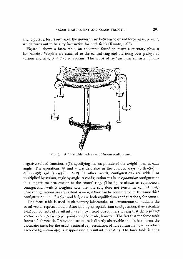
Figure 1 shows a force table, an apparatus found in many elementary physics laboratories. Weights are attached to the central ring and are hung over pulleys at various angles 0, 0 < 0 < 2~ radians. The set A of con&urntions consists of non-

FIG. 1. A force table with an equilibrium configuration.

negative valued functions a(e), specifying the magnitude of the weight hung at each angle. The operations @ and c are definable in the obvious ways: (a @ b)(B) =

a(B) + b(B) and (t * a)(0) = ta(0). I n other words, configurations are added, or

multiplied by scalars, angle by angle. A configuration a is in an equilibrium configuration if it imparts no acceleration to the central ring. (The figure shows an equilibrium configuration with 5 weights; note that the ring does not touch the central post.) Two configurations are equivalent, a N b, if they can be equilibrated by the same third configuration, i.e., if a @ c and b @ c are both equilibrium configurations, for some c.

The force table is used in elementary laboratories to demonstrate to students the usual vector representation: After finding an equilibrium configuration, they calculate total components of resultant force in two fixed directions, showing that the resultant vector is zero. A far deeper point could be made, however. The fact that the force table forms a 2-chromatic Grassmann structure is directly observable and, in fact, forms the axiomatic basis for the usual vectorial representation of force measurement, in which each configuration u(0) is mapped into a resultant force +(a). The force table is not a

292 DAVID H. KRANTZ

proper Grassmann structure, since if b is an equilibrium configuration, then a @ b N a. Apart from that, however, the underlying structures for force measurement and color measurement are fully isomorphic.

The isomorphism between color measurement and force measurement is actually more far-reaching than the above would indicate. Just as in color theory we wish to enrich the basic Grassmann structure by adding further observable relations, incorporating them into the numerical representation, so also in force theory, we must move beyond the simple observation of equilibrium or lack of equilibrium. In the case of force, the next step is to consider directional equilibrium, to constrain the acceleration of the ring to one particular direction and observe the configurations that yield an equilibrium in this partial sense. The observations of directional equilibrium yield l-chromatic Grassmann structures for each direction. This line of thinking leads eventually to the rigorous tie-in between coordinates of force vectors and coordinates of kinematic space. In color, too, one source of additional perceptual structures comes from observation of “directional equilibria” with respect to certain hue attributes. This theme will be developed in part II of this series.

Representation and Uniqueness Theorems for Grassmann Structures

Any Grassmann structure can be mapped homomorphically onto a convex cone in a vector space; this result (Theorem 1 below) uses only Axioms 1-5, not m-chromacy. If the representing vector space is chosen to be minimal, then any two such representations are isomorphic (Theorem 2, the uniqueness theorem). Finally, the representing vector space is m-dimensional if and only if the Grassmann structure is m-chromatic (Theorem 3). This formulation has the advantage of separating cleanly the roles of Axioms 1-5, which yield a (possibly infinite-dimensional) vector representation from Axiom 6, which pins down the dimensionality. It has the further advantage that the representing vector space and the homomorphism are not tied to any particular coordinate system; they are canonically constructed. The proofs are somewhat abstract. For the less algebraically minded reader, it is possible to formulate a combined theorem which can be proved by introducing coordinates early on, and that proof is sketched at the end of this subsection.

THEOREM 1. Let (A, 0, *, -) be a G rassmann structure. Then there exists a vector

space V over the real numbers, a convex cone C in V, and a function C$ from A onto C, such that for all a, b in A, t in Re+, and v in V:

(9 $(a 0 4 = d(a) + cb(b); (ii) $(t * a) = t .+(a);

(iii) a - b if and on2y if+(u) = +(b); (iv) there exist c, din A such that v = (6(c) - 4(d).

In other words, + is a homomorphism of the Grassmann structure (A, 0, *, -->


onto (C, +, ., =), where C is a convex cone in V; property (iv) guarantees that V is a minimal vector space, since any element in I’ is generated as a difference of elements 4(c), +(d) in C. Note that the Grassmann structure is proper if and only if C does not contain the zero vector of V.

THEOREM 2. Let (A, 0, *, -) be a G rassrnann structure, with two homomorphisms 4, 4’ onto convex cones C, C’ in vector spaces V, V’, satisfying (i)-(iv) of Theorem 1. Then there exists a nonsingular linear transformation T of V onto V’ such that for all a

in A, T($(a)) = $‘(a).

In other words $ is unique up to nonsingular linear transformations.

THEOREM 3. The vector space V of Theorem 1 is m-dimensional if and only if

(4 0, *, --> is m-chromatic.

The proofs of these theorems are given in the next section. But it is straightforward to prove a combined theorem by introducing coordinates. If <A, 0, C, -) is an m-chromatic Grassmann structure, choose a set of primaries a, ,..., a, . For any a

in A form Eq. (1) (with m replacing 3) and then let $(a) = (vl ,..., v,), where vi = (ui - tJ/(t - u) as in Eq. (2). Th e f unction 4 is readily shown to be a linear map onto an m-dimensional convex cone in ReTn, with a N b if and only if $(a) = 4(b).

PROOFS OF THEOREMS l-3

To construct the vector space V without using coordinates we need to introduce “differences” of elements of A. If we think of the pair (a, b) as the “difference” of a and b, we must identify equal differences. Formally, we define a binary relation % on A x A by:

(a, b) e (a’, b’) iff a @ b’ N a’ @ b.

That w is reflexive and symmetric follows immediately from (3i) and (3ii). To show transitivity of m, we require a stronger additivity property than Axiom 4, namely:

LEMMA 1. Let (A, 0) be a commutative semigroup and N be an equivalence relation on A such that a N b isf a @ c N b @ c. If a - 6, then a’ N b’ ; f f a @ a’ N b @ b’.

Proof. If a’ N b’ then

a@a’wb@a’ =a’@b Nb’@b = b @ b’.

4w=/3-3

294 DAVID H. KRANTZ

Conversely, if a @ a’ N b @ b’, then the first, second, and fourth steps of the above argument yield a’ @ b N b’ 0 b, whence a’ N b’. Q.E.D.

To show that m is transitive, suppose that (a, b) m (a’, b’) and (a’, b’) m (a”, b”). By definition of m and Lemma 1,

(a @ b’) @ (a’ @ 6”) - (a’ @b) @ (a” 0 b’).

From associativity and commutativity of @ and reflexivity and transitivity of N, we have

(a @ b”) @ (a’ @ b’) - (a” @ b) @ (a’ @ b’).

By Axiom 4, a 0 b” - a” @ b, so (a, 6) w (a”, 6”).

We now let V be the set of w-equivalence classes. Let [a, b] denote the equivalence class containing (a, b). Define operations + and . by

[a, bl + [c, 4 = [a 0 c, b 0 4

1

[t * a, t * b], if t>O;

t * [a, b] = [(-t) c b, (-t) c a], if 0 > t; [a, 4, if t = 0.

It is now completely straightforward, albeit tedious, to show that + and . are well- defined and that (V, f, .) is a vector space over the reals. In particular, [a, a] = [b, b]

for any a, b and this is the zero vector; -[a, b] = [b, a]. To construct 4 choose any fixed element e in A and let

+(u> = [a 0 e, 4.

This construction is independent of e, since for any e, e’, (a @ e, e) M (U @ e’, e’).

We make use of this freely in establishing that 4 satisfies (i) and (iii) of Theorem 1. We have

$(u @ b) = [a 0 b @ e, e]

= [u@b@e@e,e@e]

= [a 0 e, 4 + [b 0 e, 4 = m> + 4(b).

+(t * u) = [(t * u) @ (t * e), t * e]

= [t * (a @ e), t * e]

= t . [a @ e, e]

= t *d(u).


This establishes that + satisfies (i) and (ii) of Th eorem 1 and that the set C of all $(a) is a convex cone.

To prove (iii) note that

a-b i f f a@e@e-b@e@e

iff [a @ e, e] = [b @ e, e]

i f f w = M4*

For (iv), note that v = [a, b] = d(u) - 4(b). Th’ IS completes the proof of Theorem 1. To prove Theorem 2 it suffices to note that if 4, +’ are homomorphisms onto C, C’,

satisfying (i)-(iv), then T can be defined on C by T(C(a)) = $‘(a). It is trivial to show

that T is well-defined, one-to-one, additive, and positive-homogeneous. Extend T

to v by TM4 - WI = 4’(4 - +‘(4. Finally, for Theorem 3, note that an equation of form C ti * ui NC ui t ai is

equivalent (using properties (i)-(iii) of Th eorem 1) to the vector equation 1 (ti - ui) . $~(a~) = 0 in V. Thus (6i) holds i f f any m + 1 elements of C are linearly

dependent, i.e., i f f I/ has dimension at most m; and (6ii) holds i f f there exist m linearly independent elements of C, i.e., i f f V has dimension at least m.

CODES FOR GRASSMANN STRUCTURES

As an application of the preceding axiomatization I shall develop some facts about

unidimensional mechanisms or codes. These facts are mostly well known (see Brindley, 1957, 1960) but the present development illustrates the simplicity of the abstract algebraic treatment. It also provides some essential background for the next section, on dichromacy, and for the later papers in this series.

By a color code (or color mechanism in the sense of Stiles, 1967) we mean some response or function that subserves color discrimination. We can define a code to be a real-valued functionfi on A, such that iffi(u) # f#), then a is discriminable from b, ’ I.e., a N b is false. (Obviously we are ignoring imperfections in discriminability in this idealization.) Another way to look at it is as follows: define an equivalence relation

wi on A by a -i b if fi(u) =fi(b). (3)

Then mi is coarser than N, that is, a N b implies that a wi b. The converse is false of course; two lights that are not discriminated byf, may be discriminated by some other code. If metameric matches are determined by equality of absorption in three cone photopigments, then the quantum catch of a single photopigment is a code. The amount of a particular primary required for a 3-primary match is another example of a code. A third example is provided by any quantitative brightness scale (since if

296 DAVID H. KRANTZ

two lights differ in brightness, they cannot be a metameric match). The rhodopsin quantum catch is not a code, since it can be unequal for two metameric lights.

If (A, 0, *, -) is a Grassmann structure and 4 is a homomorphism of it onto (C, +, ., =>1 satisfying the conditions of Theorem 1, then any real-valued function on C defines a code on A. And, conversely, any code fi on A induces a real-valued function Fi on C: simply define Fi by Fi($(u)) = fi(u). The function Fi is well-defined because, if $(u) = +(b), then a - b, and hence by definition of a code fi(u) = fi(b). Less abstractly, we remark that for any coordinate system in the vector space V, each coordinate is a code, and any code can be written as a function Fi of the 3 coordinates.2

One of the important questions for color theory is the form of the functions that interrelate various codes. If we use three codes, +r , +2 , +a as coordinates in V, and write

for some code fi , can we pin down more precisely the function Fi ? We shall proceed to show that this can be done for certain classes of codes.

Equation (3), with its -i notation, suggests that properties of a code fi can be translated into properties of the structure (A, 0, *, wi). We already know that Axioms l-3 are true, since they deal only with (A, 0, *). What about the other three axioms of Grassmann structures ?

Some important color codes (e.g., hue) satisfy neither Axiom 4 nor 5. Others (e.g., brightness, or certain of Stiles’ 17 mechanisms) may satisfy only Axiom 5. Still others (e.g., photopigments and the Hurvich- Jameson red/green cancellation function) satisfy Axioms 4, 5, and 6 (the latter with m = 1).

Brindley (1957) called a color mechanism “substitutable” if it satisfies Axioms 4 and 5 (the additivity and scalar multiplication properties), “unidimensional” if it satisfies a version of 1-chromacy. He did not explicitly consider mechanisms for which only Axiom 5 is true, but it is interesting to do so, since they are precisely the codes for which an invariant spectral sensitivity function (Stiles, 1967) can be defined.

In what follows, every code will be assumed to satisfy 1-chromacy (Axiom 6, m = 1). A code will be termed invariant if Axiom 5 is satisfied (i.e., if fi(a) = fi(b) implies that fi(t * a) = fi(t * b)). A code is termed Grassmann if both Axioms 4 and 5 are satisfied. The next two subsections establish the form of the functions fi linking Grassmann or invariant codes to a linear coordinate system ($r , $2 , $a).

2 Actually, the above facts make no use of the 0, * structure of Axioms 4 and 5. They depend only on trichromacy, which guarantees the existence of a vector-valued mapping satisfying (iii) of Theorem 1. The same results can be obtained for any set A, and equivalence relation - on A, such that there exists a complete set of codes jr ,...,,fm , in the sense that if a - b is false, then f”(a) f f,(b) for some i. Any code for (A, --> can be written as a function of the m coordinates defined by such a complete set of codes. If topological considerations are introduced it can even be shown that any two complete sets of “independent” continuous codes contain the same fixed number of codes. But this takes us far afield.

COLOR MEASUREMRNT AND COLOR THEORY I 297

Grassmann Codes

Iffi is a Grassmann code, then (A, 0, t, wi) is a l-chromatic Grassmann structure. By Theorem 1 there exists a real-valued function pi on A such that (i) pi(a @ b) =

pi(a) + Pi(b); (ii> pi(t * a) = @i(a); and (iii) f<(a) = fi(b) if and only if pi(a) = pi(b). Clause (iii) is the same as saying that fi(a) = F&(a)), where Fi is a well-defined one-to-one function. The function pi is a linear functional on (A, 0, *) (properties i, ii); so we have just proved Theorem 4.

THEOREM 4. A code fi on a Grassmann structure (A, 0, *, -) is a Grassmann code ;f and only if fi = Fi(pi), where pi is a linear functional on <A, 0, *) and Fi is an arbitrary one-to-one function.

The linear functional pi is also a Grassmann code on (A, 0, *, -); like any code, it can be written as a function Pi of the representation 4 into the vector space V, and the function Pi is a linear functional on V, as can be trivially verified; e.g.,

PM4 + +(bN = PMa 0 4) = pi(a 0 b) = ~44 + d4 = Pi(C(a)) + Pi(+(b))*

Any linear functional on a vector space can be written as a linear combination of coordinates. So, if we introduce coordinates + = (+1 ,..., q$,J, then Pi = C qAj , for some constants olil ,.. ,, aim . Therefore we can write pi(a) = C aii$j(a), or

fda) = Fi (1 &da)). (4)

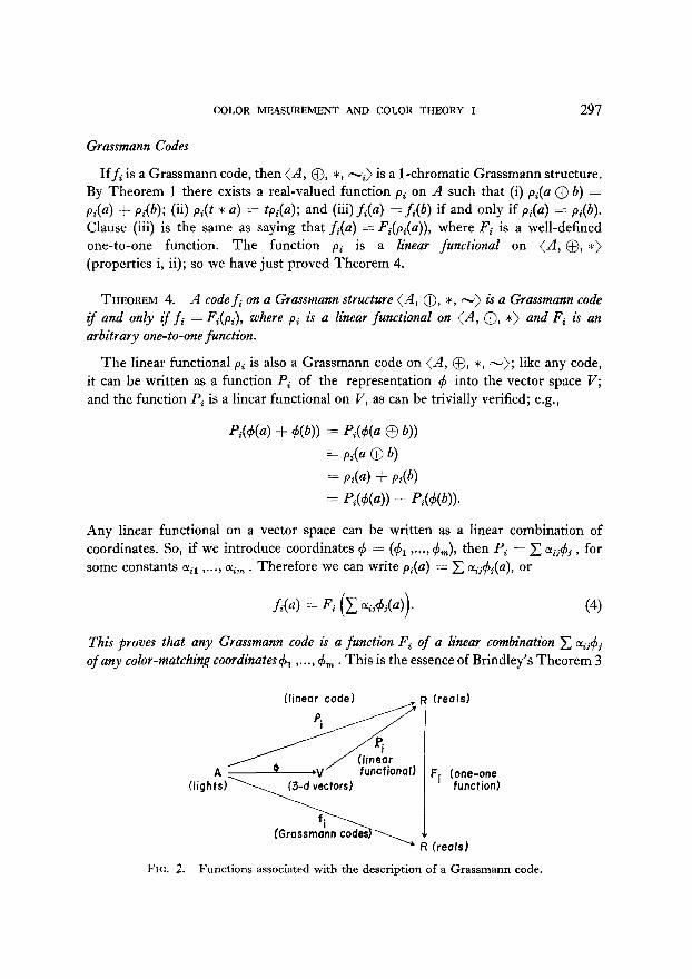
This proves that any Grassmann code is a function Fi of a linear combination C aij#j of any color-matching coordinates & , . . . , & . This is the essence of Brindley’s Theorem 3

FIG. 2. Functions associated with the description of a Grassmann code.

298 DAVID H. KRANTZ

(1960). I p t’ 1 n ar mu ar, any linear code (such as a cone-pigment quantum catch) can be written as a linear combination of color-matching coordinates.

The various functions that occur in the above description of Grassmann codes are diagrammed in Fig. 2.

Invariant Codes

If ($1 >‘..> h> are the coordinates of the representation of a Grassmann structure, then an invariant code (i.e., satisfying Axiom 5 but not necessarily Axiom 4) can be defined by any function

That is, gi is a function of the product of a linear functional, C CQ& , times a function Hi that depends only on ratios of the coordinates. Obviously if g,(a) = g,(b), then gi(t * a) = g,(t * b). The code g, possesses a sensitivity function: if one fixes b, then the sensitivity u(a) is defined by the equation g,(a) = g,(u(a) * b). This is valid for all a for which such a u(a) exists. The relative sensitivity function is independent of b, since if g,(b) = gi(r * b’), then g,(a) = gi(ru(a) * b’). The sensitivity function is a positive-homogeneous functional: u(t * a) = tu(a). It is not, however, linear, unless gi is a Grassmann code (Hz a constant). The sensitivity of a mixed light therefore cannot be calculated as an integral of the spectral sensitivity times the spectral radiance density.

The form of Eq. (5) is general: any invariant code gi can be written in that form,3 for suitably chosen Gi , Hi , and aii .

The Dual of the Grassmann Structure

In this section we point out that the Grassmann structure is determined by the set of all its linear codes. Any m independent linear functionals on the cone (A, 0, *) (determined, for example, by m photopigments or by m l-chromatic Grassmann structures) define an m-chromatic Grassmann structure, and conversely, in an m- chromatic Grassmann structure, the vector space of all linear codes is m-dimensional. The set of all linear codes for a Grassmann structure will be called the dual space of the Grassmann structure. The importance of this construction is illustrated both in the next subsection, on invariance of metameric matches, and in the final section, on dichromacy.

3 For proof, note that gl(& , t& , 3,) = Bi(t, gi($, , & , &)), where Yi is a function of two variables and where the function Bj satisfies the associativity equation 9,(tu, x) = gl(t, 9i(~, x)). The solution (Aczel, 1966, p. 329) to this functional equation is BJf, x) = Gi(tG;‘(x)). Putting H,(p, q) = GT*(g,(l, p, 4)) yields the required result.


Suppose that (A, 0, c) is a convex cone (Axioms 1 and 2 hold). Then any m linear functionals on A define a Grassmann structure: given linear functionals p1 ,..., pm , define wp by

a Np b if and only if pi(a) = pi(b), i = I,..., m.

The proofs that Axioms 3-5 hold are trivial, and in addition, it is easy to show that <A, 0, *, --,> is m-chromatic provided that pr ,..., pm are linearly independent. (Otherwise it is n-chromatic, with n < m.) To prove this, just note that $(a) =

(~&4-v PA >) . a IS a h omomorphism satisfying (i)-(iv) of Theorem 1. (This construction can also be used to prove Brindley’s Theorem 2, 1957.4) By Theorem 4, any linear functional on (A, 0, x) which is a code for N,, is a

linear combination of pr ,..., pm . Therefore the space of all linear functionals which are codes is m-dimensional for an m-chromatic Grassmann structure. We summarize these results by

THEOREM 5. Let (A, 0, *) be a convex cone. Let P be any m-dimensional space of linear functionals on A. Let a N b if and only ;f pi(u) = pi(b) for all pi in P. Then

(A, 0, *r --> is an m-chromatic Grassmann structure. Conversely, the set of linear functionals on (A, 0, +> that are codes for an m-chromatic Grassmann structure form an m-dimensional linear space, called the dual space.

The Three-Pigment Hypothesis

One obvious source of linear functionals over (A, 0, *) comes from photopigments: if a = a(h) is a spectral radiance density and pi(X) is a photopigment spectral absorption function, then

pi(a) = s

WA) pi(A) dx

4 Brindley dealt with a related but slightly more subtle problem. Given an m-chromatic matching relation -,, determined by linear functionals pi ,..., pm, and given another matching relation - which includes -p, under what circumstances does the reverse implication hold, from - to mp? Under what circumstances, in other words, are pi ,..., pm codes for -? His answer was as follows. If a -b, where a = a, @ ... @I a, and b = a,+i @ ... @ a,,, , and if there is no other match of form &,I tj * ai - CjcJ I II. i aj, where the index sets I, / do not overlap, then a wp b. The proof is immediate: By m-chromacy of (A, 0, *, -J there exists some -0 match of the form given in Eq. (l), and by additivity of wp , the match can be reduced to disjoint form. But an -0 match implies an - match; therefore, by uniqueness of the latter match, we must have a -P . b If we accept uniqueness of color matching, and the proposition that any three monochromatic lights are linearly independent (so that all color matches involve m + 1 = 4 distinct components), then this would permit us to argue from the existence of 3 “receptor mechanisms” satisfying substitutability to the conclusions that color matching is additive and that the 3 receptor mechanisms are Grassmann codes.

300 DAVID H. KRANTZ

is a linear functional, proportional to total quantum catch. Brindley (1970) and others contrast the three-pigment hypothesis- that metameric matches are determined by three codes which are photopigment functionals-with multipigment, three mechanism hypotheses, in which three independent linear codes (br , $a, 4s are related to n independent photopigment functions p1 ,..., pn by equations

(6)

One of the motivations for this hypothesis is the idea (MacAdam, 1956) that adaptation effects can be described by linear transformations in an n-dimensional space, with n > 3. More precisely, let wP and N be defined by p1 ,..., p,, and by $r ,

$2 9 $3 Y respectively, and let V/n and Va be the corresponding vector spaces (Theorem 1). Equation 6 defines a linear transformation K of V, onto I’, , satisfying K(p(a)) = $(a). MacAd am’s idea was to describe an adaptation change by a linear transformation X of V, onto itself, so that light a, in adaptation 1, matches light b, in adaptation 2, if and only if

W(P(4)) = k’(PW = cw (7)

(Actually, MacAdam proposed the more specific von Kries coefficient principle, whereby the transformation X is defined by [Xp(a)li = asps.)

The difficulty with this idea, as pointed out by MacAdam and others, is that metameric matches are invariant under the sorts of adaptation that are in question. Since a N b if and only if K(p(a)) = K(p(b)), we see that Q N 6 if and only if p(u) - p(b) is in the (FZ - 3)-dimensional null space NK of the transformation K. Since metameric matches are invariant, we have X(p(a)) - X(p(b)) also in NK ; that is, X maps NK onto itself. We can therefore define a linear transformation U on I’, that describes adaptation just as well as X on V, does: let

V~(PW)) = W(P(4)). (8)

This is well-defined because, as just noted, if K(p(u)) = K(p(b)), then K( X(p(u))) = K( X(p(b))). The transformation U describes adaptation because, by (7) and (S), light a in adaptation 1 matches light b in adaptation 2 if and only if U($(b)) = +(a).

We have shown, then, that the multipigment hypothesis cannot be used to solve MacAdam’s problem; if adaptation can be described by the linear transformation X in V,, then it can be described just as well by the linear transformation U in Va . An n-pigment system can exist, with n > 3, but in such a case, the linear transformations of I’, that leave metameric matches invariant are precisely the ones that map NK, an (n - 3)-dimensional subspace of V, , into itself. In the particular case of the von Kries law, considered by MacAdam, the linear codes pi are the dual basis for a set


of distinct eigenvectors of T. Therefore n - 3 of the eigenvectors must be in NK, i.e., are mapped into zero by K; this means that in Eq. (6), the & depend only on the remaining three pi . So if the von Kries law holds, then we are forced back to the three-pigment hypothesis.5

REDUCTION DICHROMACY

Suppose now that in addition to a trichromatic Grassmann structure (A, 0, *, -->, we have an additional matching relation, say wP , the protanopic color-matching relation. The simplest situation arises when (A, 0, *, wP) is a dichromatic Grassmann structure such that N is included in wP: that is, the typical normal match is also a match for the dichromat. This is called reduction dichromacy. In that case, the mapping Tp: [a, b] -+ [a, blP is a natural homomorphism of the canonical vector space V, defined from the normal relation N, onto the canonical vector space VP , defined from mP . The null space of this homomorphism is a one-dimensional subspace of Y, we denote a generator of that space by nP. This vector is called the protanopic confusion center.

In terms of linear functionals, any linear code for wP is also a code for N, hence, the dual space (space of linear codes) for mP is a two-dimensional subspace of the three-dimensional dual of N (see Th eorem 5). It can be thought of as the space of codes that are null on V, . Any linear code for -which is not in the subspace (not a code for wP) can be thought of as a “lost” code for the protanope.

If we choose two independent linear codes for mP , denoted pi , pz , and a third code p3 for N which is independent of the first two, then p = (pl , pz , p3) is a coordinate system for V such that (pl , pJ is a representation for wP . In terms of the goal of enriching the original Grassmann structure, we have achieved a new structure

(A, 0, *, -, -p>, and a representation (pl , pz , p3) that handles both N and mP in a natural way. The uniqueness theorem is given by the matrix equation

i.e., there are 7 free parameters, with the restriction that (o~ii(~~~ - 01~~01~~) c~aa # 0. (Obviously one can choose any two linear functionals on VP , pl’, p2’, with 4 free parameters, and then the choice of p3 ’ is entirely arbitrary, except that it must be independent of pl’, pz’.)

If we have two distinct dichromatic matching relations, say, wP and wD, each

5 There are several incorrect proofs of this in the literature. The present argument, for the case of the van Kries law and invariant metameric matches, may be found in Krantz (1968).

302 DAVID H. KRANTZ

satisfying the above conditions, then we have homomorphisms Tp , T, , with distinct (linearly independent) null spaces generated by vP , ho . The corresponding subspaces of linear codes intersect in a unique (up to change of unit) code p1 ; this can be thought of as the linear functional whose null space is generated by vP and vD . We can then

choose p2 which is a code for wP but not me and pa with the opposite property.

We now have a representation (pl , pz , p3) for (A, 0, *, N, mP , we) such that (pl , pz) provide a representation for wP and p1 , p3 for -D . This is unique up to

Note that N, “P , and wD together suffice to determine the common code for these

three types of observer, uniquely up to change in unit. Though pa is a code which is missing for in , it is not the missing code-in fact, it is meaningless to speak of the missing code, since any linear combination of p1 , pz , p3 which has nonzero coefficient for pa will define a code for N which fails to be a code for wD .

Finally, if there are three types of reduction dichromacy represented by mP , -e , and -TY with linearly independent confusion centers vP , v,, , and vT , then we can select6 three unique codes, p1 common to all but wT, pz common to all but we , and ps common to all but wP . The uniqueness theorem permits only diagonal transformations.

A recent specification of three unique codes, on this basis, is found in Vos and Walraven (1971).

It should be noted that nothing in this development suggests that a code which is

common to normals and two types of dichromats, (but missing for the third type) has any special physiological status. For example, in the commonly encountered fusion theory of protanopia and deuteranopia, it is postulated that there are three photopigment codes, p1 , pz , p3, which subserve normal color vision, but that protanopes and deuteranopes have p2 and p3 fused into respective linear combinations papa + p3p3 and vzpz + v3p3. Assuming the tritanope simply loses p1 , the 3 codes

which give a common representation for (A, 0, *, N, mP, ho, wT) are pl,

p2p2 + w3p3, and y2p2 + sj3p3. Th us pzp2 + p3p3 is common to normals, tritanopes, and protanopes, but it has special physiological status only for protanopes. A more extensive example can be constructed in which each dichromat has two codes, both fusions of the 3 normal pigments; none of the 3 unique codes would have “real” status for any of the 4 types of observers. These unique codes are constructs which neatly describe the confusions that dichromats make; nothing else. However, other lines of evidence now indicate that the three main types of dichromacy do in fact

6 The construction here is the well-known selection of a dual basis to (up, uD, or).


arise from single photopigment losses; in that case, the unique code for -, wP , -D , which is missing in mT , corresponds to the actual physiological loss in wT . Even such a loss theory, however, does not tell which recombinations of the remainng pigments may serve as the functional codes.

REFERENCES

ACZEL, J. Lectures on functional equations and their applications. New York: Academic Press, 1966. BEALS, R., KRANTZ, D. H., & TVERSKY, A. Foundations of multidimensional scaling. Psychological

Review, 1968, 15, 127-142. BRINDLEY, G. S. Two theorems in colour vision. Quarterly Journal of Experimental Psychology,

1957, 9, 101-105. BRINDLEY, G. S. Two more visual theorems. Quarterly Journal of Experimental Psychology, 1960,

12, 110-112. BRINDLEY, G. S. Physiology qf the retina and the visual pathway. 2nd ed. London: Edward

Arnold, 1970. GRASSMANN, H. Zur Theorie der Farbenmischung. Poggendorffs Annalen der Physik, 1853, 89,

69-84. (English translation, On the theory of compound colours, Philosophical Magazine (London), 1854, Series 4, 7, 254-264.)

HURVICH, L. M., & JAMESON, D. An opponent-process theory of color vision. Psychological Review, 1957, 64, 384404.

KBNIG, A., & DIETERICI, C. Die Grundempfindungen in normalen und anormalen Farben- systemen und ihre Intensitatsvertheilung im Spectrum. Zeitschrift fiir Psychologie und Phy- siologie der Sinnesorgane, 1892, 4, 241-347.

KRANTZ, D. H. A survey of measurement theory. In Mathematics of the decision sciences, Part 2, G. B. Dantzig & A. F. Veinott, Jr. (Eds.), Lectures in applied mathematics. Vol. 12. Providence: American Mathematical Society, 1968.

KRANTZ, D. H. Color measurement and color theory. II. Opponent-colors theory. Journal of Mathematical Psychology, 1975, 12, --.

KRANTZ, D. H. Fundamental measurement of force and Newton’s first and second law-s of motion. Philosophy of Science, 1973, 40, 481-495.

LAmn~rxR, J., KRANTZ, D. H., & CICERONE, C. Opponent-process additivity. 1. Red/green equilibria. Vision Research, 1974, 14, 1127-l 140.

LARIMER, J., KRANTZ, D. H., & CICERONE, C. Opponent-process additivity. II. Yellow/blue equilibria and nonlinear models. Vision Research, 1975, 15, 723-731.

MACADAM, D. L. Chromatic adaptation. Journal of the Optical Society of America, 1956, 46, 500-513.

STILES, W. S. Mechanism concepts in colour theory. Journal of the Colour Grotdp, 1967, 105-I 23. THOn4SON, L. C. Fovea1 color sensitivity. Namre, 1946, 157, 805. TVERSKY, A., & KRANTZ, D. H. The dimensional representation and the metric structure of

similarity data. Jozrrnal of Mathematical Psychology, 1970, 7, 572-596. Vos, J. J., & WALRAVEN, P. L. On the derivation of the fovea1 receptor primaries. b’ision Research,

1971, 11, 799-818.

RECEIVED: November 21, 1974

Documents

Color Measurement and Color Theory: I - Deep Blue