Collusive Price Rigidity under Price-Matching

Punishments∗

Luke Garrod†

March 2012

Abstract

By analysing an infinitely repeated game where unit costs alternate stochas-

tically between low and high states and where firms follow a price-matching

punishment strategy, we demonstrate that the best collusive prices are rigid

over time when the two cost levels are sufficiently close. This provides game

theoretic support for the results of the kinked demand curve. In contrast to

the kinked demand curve, it also generates predictions regarding the level and

the determinants of the best collusive price, which in turn has implications

for the corresponding collusive profits. The relationships between such price

rigidity and the expected duration of a high-cost phase, the degree of product

differentiation, and the number of firms in the market are also investigated.

Keywords: Tacit collusion, kinked demand curve, price rigidity

JEL: L11, L13, L41

1 Introduction

The old theory of the kinked demand curve (Hall and Hitch, 1939; and Sweezy, 1939)

was the first attempt to formalise the long-standing belief that tacit collusion and

price rigidity are linked. It assumes that there is a prevailing focal price and that

rivals will match a firm’s price decrease but they will not match a price increase.

This rivalry implies that each firm’s demand curve has a kink at the focal price,

and it follows from the resultant discontinuity in marginal revenue curve that prices

remain constant at the focal level for a range of marginal costs. Although the rivalry∗I am grateful for comments from Iwan Bos, Steve Davies, Joe Harrington, Morten Hviid, Roman

Inderst, Kai-Uwe Kühn, Bruce Lyons, Matt Olczak, Patrick Rey, Paul Seabright, Chris M. Wilson,two anonymous referees, and seminar participants at the International Industrial OrganizationConference 2011 and the European Association of Research in Industrial Economics Conference2011. The support of the Economic and Social Research Council (UK) is gratefully acknowledged.The usual disclaimer applies.

†School of Business and Economics, Loughborough University, Loughborough, Leicestershire,LE11 3TU, United Kingdom, email: l.garrod@lboro.ac.uk

1

CORE Metadata, citation and similar papers at core.ac.uk

Provided by Loughborough University Institutional Repository

of the kinked demand curve has an intuitive appeal and some anecdotal support,

this theory has been heavily criticised (for example see Tirole, 1988, p.243-245).

Contemporary models of dynamic oligopolistic interaction differ in two respects

with the kinked demand curve. First, they are modelled as an explicit dynamic

game using the theory of repeated games, where collusive prices are sustainable

when the short-term gain from any deviation is outweighed by the long-term loss

from a credible retaliation. Second, firms usually more than match lower deviation

prices, because the most commonly analysed retaliations are “Nash reversion” (see

Friedman, 1971) and “optimal punishment strategies” (see Abreu, 1986, 1988). Us-

ing such models, there is a theoretical literature that analyses the effect of temporary

changes in market conditions on the best collusive prices that achieve the highest

levels of profit possible (for example see Rotemberg and Saloner, 1986; Haltiwanger

and Harrington, 1991).1 A feature of this literature is that, barring the special cir-

cumstances when incentives are perfectly aligned, the best collusive prices are not

rigid over time. This is at odds with the results of the kinked demand curve and

with the belief that tacit collusion and price rigidity are linked.

In this paper, we analyse the rivalry of the kinked demand curve in an infinitely

repeated game and show that, in contrast to the previous collusion literature, the

best collusive prices can be rigid over time despite small industry-wide changes in

unit costs. This provides game theoretic support for the results of the kinked de-

mand curve. We derive this result by extending Lu and Wright (2010) who analyse

an infinitely repeated game where, similar to the kinked demand curve, firms match

lower deviation prices (provided they are above the one-shot Nash equilibrium price)

but do not match higher deviation prices. They show that collusive prices are sus-

tainable under such “price-matching punishments” when products are symmetrically

differentiated and when market conditions do not vary over time. We extend their

model so that unit costs alternate stochastically between high and low states, and

analyse the characteristics of the best collusive subgame perfect Nash equilibrium

when prices are rigid over time.

The intuition behind price rigidity in our model is that when unit costs are

temporarily high today and they are permanently low in the future, there is an

incentive to deviate today from any collusive price above the collusive price that

prevails in the future. The reason is that when a firm deviates to that future price

today, there is no long-term loss to offset the deviation gain, because the punishment

is just to match the deviation price, which still results in the collusive price being set

in the future. An implication of this is that the best collusive prices are rigid when

the two cost levels are sufficiently close, such that the one-shot Nash equilibrium

1Although much of the previous literature focuses on changes in demand, many of the resultsgeneralise to changes in costs.

2

price of the high-cost state is not above the future collusive price. When high costs

persist into the future, price matching such a deviation does reduce the profits of

future high-cost states, but this long-term loss must outweigh the initial gain for

procyclical prices to be sustainable. Given this loss is small and the gain is large

when the two cost levels are close, the best collusive prices are rigid over time when

the difference between the two cost levels is below some critical threshold. We show

that this critical threshold falls as high-cost states are likely to persist for longer

into the future, and it equals zero when the high-cost state is expected to last

permanently.

In contrast to the kinked demand curve, our model generates predictions regard-

ing the level of the best rigid price and the effects of the other parameters of the

model on it. This price uniquely achieves the highest level of profit possible, given

that the price does not vary over time. It defines the best collusive price in both cost

states when the difference between the two cost levels is below the critical threshold,

and it is always between the one-shot Nash equilibrium price of the high-cost state

and the monopoly price of the low-cost state for such conditions. The best rigid price

is determined by the incentives to collude in low-cost states, and it monotonically

increases with the level of high costs at a rate that is less than one-to-one. An im-

plication of these features is that when the best collusive prices are rigid over time,

the resultant per-period collusive profits of low-cost states are strictly increasing in

the level of high costs, but such profits of high-cost states are strictly decreasing in

the level of high costs. In contrast, the corresponding present discounted values of

collusive profits are strictly decreasing in the level of high costs, whether the initial

period has high or low costs.

Our model also generates predictions regarding the relationship between price

rigidity and the number of firms in the market, which has been investigated by several

empirical studies (for example see Carlton, 1986, 1989). This relationship ultimately

depends upon the degree of product differentiation. Based on an example where

demand is derived from the constant elasticity of substitution version of Spence-

Dixit-Stiglitz preferences (Spence, 1976; and Dixit and Stiglitz, 1977), we show

that the best collusive prices are rigid for the largest difference between the two

cost levels when products are differentiated by an intermediate degree. This is

because price-matching punishments do not support collusive prices when products

are homogeneous, and since firms can set the monopoly prices when they have no

close rivals. Finally, we find that the best collusive prices are rigid for a larger

difference between the two cost levels in a concentrated market, with few firms,

than in a less concentrated market, with a greater number of firms, when the degree

of product differentiation is sufficiently low.

The rest of the paper is structured as follows. Section 2 reviews the related

3

literature and provides anecdotal support for a link between price matching and

price rigidity. Section 3 outlines the assumptions on demand and costs, and it

formally defines the price-matching punishment strategy. In section 4, we first find

the conditions for which the best collusive prices are rigid over time. We then analyse

the relationship between such price rigidity and the expected duration of a sequence

of high-cost states, and after that we investigate the effects of such price rigidity and

fluctuating costs on the best collusive profits. Section 5 places more structure on

demand to investigate the effects of both the degree of product differentiation and

the number of firms in the market on such price rigidity, and section 6 concludes.

All proofs are relegated to the appendix.

2 Related Literature and Evidence

In this paper, we propose that the expectation that lower deviation prices will be

matched can lead to price rigidity during collusive phases, and there is some anec-

dotal support for a link between the two. Slade (1987, 1992) analysed a price war

between gasoline retailers during 1983 in Vancouver (see also Slade, 1990). She

found that there was “a high degree of (lagged) price matching during the war” and

that “prices before and after the war were uniform across firms and stable over time”

(1992, p.264). In fact, “after the price war came to an end, prices were stable for

nearly a year” (1987, p.515). Slade (1989, p.295) also argues that other Canadian

markets (including nickel, cigarette, as well as gasoline) had three stylised facts:

“First, price is the choice variable and it can be observed by all. Second, price wars

are occasional events and are separated by periods of stable prices. Third, during

a war there is considerable matching of prices”. Similarly, Kalai and Satterthwaite

(1994) state that between 1900 and 1958 small firms in the US steel industry believed

that the largest producer would match their prices if they undercut it, and observed

that “Before World War II certain classes of steel products showed remarkable price

rigidity” (p.31).2

The anecdotal evidence above suggests that, in at least some situations, price

matching is a relevant form of firm behaviour, and this is re-emphasised by Slade’s

(1987) empirical evidence that finds some support for strategies, similar to price

matching, where “small deviations lead to small punishments” over Nash reversion

(p.499). This contrasts with the informal reasoning that argues that since collusion

is easier to sustain under harsher punishments, then colluding firms would employ

the harshest credible punishment. The evidence above also suggests that our price

2Levenstein (1997) and Genesove and Mullin (2001) also find that some cartel price wars consistedof mild punishments and price matching, respectively, but due to infrequent price observations it isnot possible to determine the extent to which prices vary over time.

4

rigidity result may be of some empirical relevance for such situations where price

matching is prevalent. This differs to previous attempts to model the rivalry of the

kinked demand curve in dynamic settings, because they do not find a link between

price matching and price rigidity.3

Our model also contrasts with the literature that analyses collusion when mar-

ket conditions vary over time. Rotemberg and Saloner (1986) show that under Nash

reversion the deviation gains are greatest in a temporary boom but the long-term

losses are constant when future market conditions are independent of current condi-

tions. This implies that any price that is just sustainable in a low-cost boom is easier

to sustain in a high-cost bust, so the best collusive prices are procyclical. For similar

reasons, the incentive to deviate from a rigid price is greatest in a period of low costs

under price-matching punishments, when future fluctuations in costs are indepen-

dent of or positively correlated with the current level. However, procyclical collusive

prices may not be sustainable, because there is a discontinuity in the incentives to

collude at the rigid price in high-cost states. This is because price matching reduces

only the price set in future high-cost states when a firm deviates in a period of high

costs by reducing its price to the low-cost price that prevails in low-cost periods.

Therefore, such a deviation from a price above yet very close to the low-cost price

can generate a much smaller long-term loss than an otherwise identical deviation

from the low-cost price, where price matching reduces the prices set in all future

periods. Yet, the deviation gains are effectively the same for such deviations. As

a result, a deviation in a period of high costs from a price only slightly above the

low-cost price can be profitable, even though a deviation from the low-cost price will

be strictly unprofitable.

Finally, this paper is also related to Athey et al (2004) who develop an alterna-

tive model of collusive price rigidity, where prices are publicly observable but firms

experience private shocks to their unit costs in each period. They show that the

best collusive prices under Nash reversion may be rigid over time because, although

demand is not allocated to the most efficient firm, this inefficiency can be outweighed

by the benefit of detecting deviations easily.4 Their model is similar to Green and

Porter (1984) since, due to some information asymmetry, price wars can occur on

3Bhaskar (1988) and Kalai and Satterthwaite (1994) show that price rigidity does not occur ina one-shot game when lower prices can be matched immediately before profits are realised. In aninfinitely repeated game where a duopoly alternates between committing to price for two periods,Maskin and Tirole (1988) show that price rigidity can occur in a Markov perfect equilibrium whencosts fall permanently, because firms attempt to avoid a price war. However, this is because rivalsmore than match lower prices. In another related infinitely repeated game, Slade (1989) capturesthe three stylised facts discussed above when an unexpected change in demand is anticipated to bepermanent, but stable prices only occur in her model when the new equilibrium is reached.

4 In a similar model, Hanazono and Yang (2007) show that price rigidity can also occur withunobservable demand fluctuations.

5

the equilibrium path when firms receive a bad signal. In contrast, price wars do not

occur on the equilibrium path in our model, because there is symmetric information.

Instead, the successfulness of collusion is affected by market conditions in a simi-

lar way as Rotemberg and Saloner (1986). Our model adds to our understanding of

price rigidity because it is the first to consider the relationship between price rigidity

and the degree of product differentiation, and it can be tested empirically since it

does not rely on parameters that are likely to be unobservable to an econometrician.

3 The Model

3.1 Basic assumptions

Consider a market where a fixed number of n ≥ 2 firms each produce a single

differentiated product and compete in observable prices over an infinite number of

periods. In any period t, firms have constant unit costs, ct ≥ 0, face no fixed costs,and have a common discount factor, δ ∈ (0, 1). They simultaneously choose price ineach period and the demand of firm i = 1, . . . , n in period t is qi(pit,p−it, n) wherepit is its own price and p−it is the vector of its rivals’ prices. Demand is symmetric,strictly decreasing in pit and limpit→∞ qi(pit,p−it, n) = 0. Since firms are symmetric,at equal prices pit = pt for all i, qi(pt, pt, n) = q(pt)/n where q(pt) is independent of

n. For every price vector pt=(pit,p−it) where qi(pit,p−it, n) > 0 for all i, demandis twice continuously differentiable and from Vives (2001, p.148-152) we assume it

has the following standard properties:

Assumption 1. ∂qi∂pit

> j=i∂qi∂pjt

> 0

Assumption 2. ∂2qi∂pit∂pjt

≥ 0 ∀ j = i

Assumption 3. ∂2qi∂p2it

+ j=i∂2qi

∂pit∂pjt< 0.

These assumptions imply that products are imperfect substitutes, demand ex-

hibits increasing differences in (pit, pjt) and the own effect of a price change domi-

nates the cross effect both in terms of the level and slope of demand.

Firm i’s per-period profit in period t is πit(pit,p−it; ct, n) = (pit−ct)qi(pit,p−it, n),where at equal prices pit = pt for all i write πit(pt, pt; ct, n) = πt(pt; ct, n). Assump-

tions 1 and 2 imply that prices are strategic complements:

∂2πit∂pit∂pjt

> 0 ∀ j = i ∀ t. (1)

6

Since unit costs are constant in any period, Assumptions 1 and 3 are sufficient to

ensure the best reply mapping is a contraction (see Vives, 2001, p.150):

∂2πit∂p2it

+j=i

∂2πit∂pit∂pjt

< 0 ∀ t. (2)

This guarantees the existence of a unique one-shot Nash equilibrium price in pure

strategies, denoted pN (ct, n). It follows from (1) and (2) that each firm’s per-period

profit is strictly concave in its own price (i.e. ∂2πit/∂p2it < 0), which implies that if

rivals charge a price above pN (ct, n), then a firm can strictly increase its per-period

profit by unilaterally lowering its price towards the one-shot Nash equilibrium price

(i.e. ∂πit/∂pit < 0 ∀ pjt > pN (ct, n), j = i). Assumption 1 guarantees that pN (ct, n)is strictly increasing in ct and to ensure that pN (ct, n) is strictly decreasing in n, we

assume the following sufficient condition:

Assumption 4. ∂2qi∂pit∂n

< 0.

Finally, to ensure that the monopoly price, pm(ct), is unique with pm(ct) >

pN (ct, n) we assume:

Assumption 5. d2πtdp2t

= ∂2πit∂p2it

+ 2 j=i∂2πit∂pit∂pjt

+ ∂2πit∂p2jt

< 0 ∀ t.

An implication of Assumption 5 is that if all firms set the same price below the

monopoly price, then they would strictly increase their per-period profits if all set

a higher price (i.e. dπt/dpt > 0 ∀ pN (ct, n) ≤ pt < pm(ct)). Assumption 1 ensuresthat pm(ct) is strictly increasing in ct, while the symmetry assumptions on demand

and costs guarantee that pm(ct) is independent of n.

3.2 Cost fluctuations

In any period, unit costs can be low or high such that ct = 0 or ct = c > 0. To

simplify notation, write pN (0, n) = pN (n), pm(0) = pm and πit(pit,p−it; 0, n) =πit(pit,p−it;n). The current level is common knowledge before firms set prices, andexpectations of future levels of ct for all t follow a Markov process such that:

λ ≡ Pr (ct = c| ct−1 = 0) ∈ (0, 1)θ ≡ Pr (ct = 0| ct−1 = c) ∈ (0, 1)μ ≡ Pr (c0 = c) ∈ [0, 1].

7

Thus, λ is the transition probability associated with moving from a low-cost state

to one of high costs, and θ is the probability that corresponds with a transition from

high costs to low costs. The parameter μ describes how the system begins.

This process implies that the probability that costs will be high in the next

period is λ if they are currently low, otherwise it is 1 − θ. Thus, future costs are

independent of the current level if 1 − θ − λ = 0, and this simple case provides a

benchmark for our analysis. In many industries it is natural to expect that future

costs will be positively correlated with the current level. Consequently, we also

allow for the case where 1 − θ − λ > 0, which implies that it is more likely that

the current cost level will continue into the next period than change. Following the

terminology of Bagwell and Staiger (1997), we refer to the former as zero correlation

(1− θ − λ = 0) and the latter as positive correlation (1− θ − λ > 0).

3.3 Collusive prices and profits

Due to the Markov process that determines future cost levels, collusive profits are

the same in any high-cost state regardless of the specific date, other things equal,

and likewise for any low-cost state. Thus, the best collusive prices emerge as a pair,

and we wish to find the conditions for which these are equal. Analysing the best

collusive prices is consistent with the prominent papers in the collusion literature

(for example see Rotemberg and Saloner, 1986; Haltiwanger and Harringtion, 1991),

and it is also consistent with the kinked demand curve since the most profitable

equilibrium is often argued to be the most logical (see Tirole, 1988, p.244).

Let the collusive prices of high- and low-cost states be p(c) and p(0), respectively,

and denote ΩH(p(c), p(0)) as a firm’s expected discounted profit in period t and

thereafter, if period t is a high-cost state. Similarly, denote ΩL(p(0), p(c)) as a

firm’s expected discounted profit in period t and thereafter, if period t is a low-cost

state. Suppressing notation slightly, it is possible to write such profits as:

ΩH = π(p(c); c, n) + δθΩL + δ(1− θ)ΩH

ΩL = π(p(0);n) + δλΩH + δ(1− λ)ΩL.

Solving for ΩH and ΩL gives:

ΩH(p(c), p(0)) = π(p(c); c, n) + δ1−δ

θωπ(p(0);n) + (1− θ

ω )π(p(c); c, n)

ΩL(p(0), p(c)) = π(p(0);n) + δ1−δ [

λωπ(p(c); c, n) + (1− λ

ω )π(p(0);n)],

where ω ≡ 1−δ(1−θ−λ) > 0, 0 < θω < 1 and 0 <

λω < 1. The first terms on the right

hand-side of the above equations represent the profits from the initial periods, and

the second terms represent the discounted profits from all future periods, conditional

8

on expectations of future cost levels.

3.4 Punishment strategy

Drawing on the insights of Lu and Wright (2010), we assume that firm i’s price-

matching punishment strategy profile for all t is of the form:

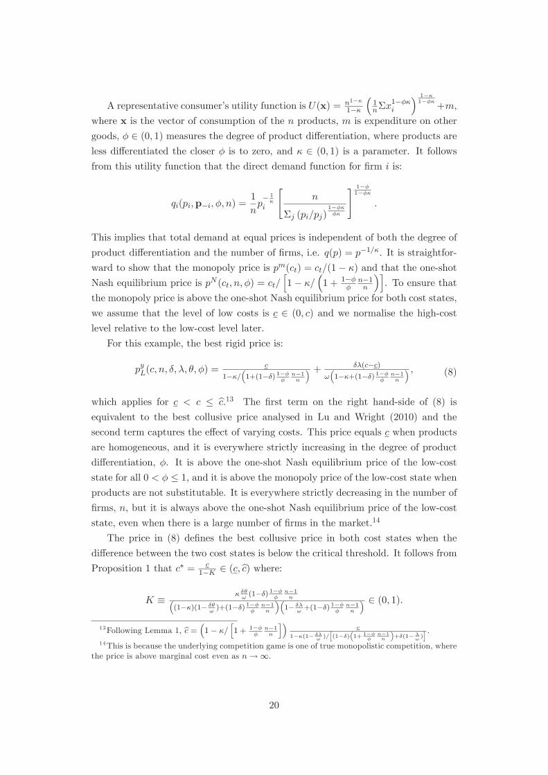
pi0 = p0(c0) = p(c0)

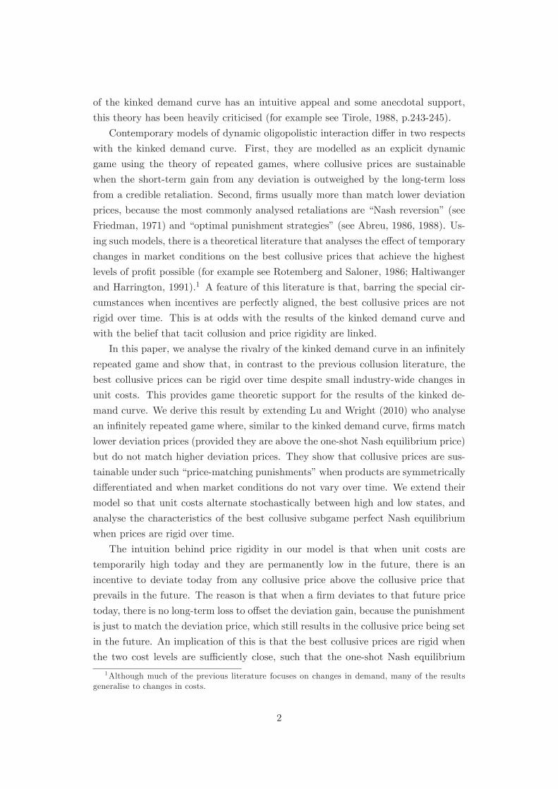
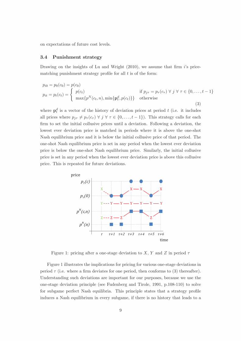
pit = pt(ct) =p(ct) if pjτ = pτ (cτ ) ∀ j ∀ τ ∈ {0, . . . , t− 1}max{pN (ct, n),min{pdt , p(ct)}} otherwise

(3)

where pdt is a vector of the history of deviation prices at period t (i.e. it includes

all prices where pjτ = pτ (cτ ) ∀ j ∀ τ ∈ {0, . . . , t − 1}). This strategy calls for eachfirm to set the initial collusive prices until a deviation. Following a deviation, the

lowest ever deviation price is matched in periods where it is above the one-shot

Nash equilibrium price and it is below the initial collusive price of that period. The

one-shot Nash equilibrium price is set in any period when the lowest ever deviation

price is below the one-shot Nash equilibrium price. Similarly, the initial collusive

price is set in any period when the lowest ever deviation price is above this collusive

price. This is repeated for future deviations.price

timepN(c,n)

+1ZpN(n) ZYY

Xp (c)

+2 +3 +4 +5 +6

X XXY Y Y Y YZ Z

p (0)

Figure 1: pricing after a one-stage deviation to X, Y and Z in period τ

Figure 1 illustrates the implications for pricing for various one-stage deviations in

period τ (i.e. where a firm deviates for one period, then conforms to (3) thereafter).

Understanding such deviations are important for our purposes, because we use the

one-stage deviation principle (see Fudenberg and Tirole, 1991, p.108-110) to solve

for subgame perfect Nash equilibria. This principle states that a strategy profile

induces a Nash equilibrium in every subgame, if there is no history that leads to a

9

subgame in which a deviant will choose an action that differs to the one prescribed by

the strategy, then conform to the strategy thereafter (assuming the deviant believes

others will also conform to the strategy). Thus, to prove subgame perfection, it

suffices to show that a one stage-deviation is not profitable in the initial collusive

subgames and nor are such deviations in every possible punishment subgame. We

say that collusive prices are supportable if the strategy profile in (3) is a subgame

perfect Nash equilibrium for all i = 1, . . . , n.

The collusive prices are initially procyclical in Figure 1, because firms set pτ (c)

and pτ (0) in high- and low-cost states, respectively. If a firm deviated to Y in period

τ , then Y is matched thereafter. If it deviated to Z, however, then Z is matched in

future low-cost states, otherwise pN (c, n) is set. Departing slightly from the kinked

demand curve but consistent with Lu and Wright (2010), firms do not match prices

below pN (ct, n) in period t because doing so seems unreasonable. This assumption is

not crucial in determining the range of rigid prices for which collusion is sustainable

or the parameter space where the best collusive prices are rigid. This is because a

deviation to Z is always less profitable than a deviation to Y in a period of low costs

when the best collusive prices are rigid, and a deviation to Z would never occur in

a period of high costs, even for prices that are not supportable. This assumption

ensures that (3) defines a Nash equilibrium in punishment subgames for histories

where the lowest ever deviation price is below pN (ct, n) in period t, and that it is

possible to check that (3) induces a Nash equilibrium in punishment subgames that

start with a period of low costs for histories where the lowest deviation price is

between pN (n) and pN (c, n).

The strategy profile (3) also has a similar feature for one-stage deviations to

prices above the lowest initial collusive price, because if a firm deviated to X, then

X is matched only in periods when the initial collusive price is above X, otherwise

pτ (0) is set. Figure 1 illustrates the case for procyclical prices, but it equally applies

to the case of countercyclical prices (where pτ (c) is set in low-cost states and pτ (0)

in high-cost states). This resembles the rivalry of the kinked demand curve, where

firms do not match price increases. This is because for deviations where a firm raises

its price from pτ (0) to a price above pτ (0), the deviation is never matched in future

low-cost states and it is also not matched in future high-cost states when there is

price rigidity. A slight difference is that X is not matched in future low-cost states,

if prices are procyclical and a firm lowered its price from pτ (c) to X in period τ .

However, the rationale for the strategy is the same: each firm expects to lose sales,

if it set X in periods when its rivals are expected to set pτ (0).5

5An alternative strategy is one where downward deviations from pt(c) to X are matched in allfuture periods, other things equal. Since this alternative and (3) are equivalent for rigid prices, therange of rigid prices sustainable and the characteristics of the best rigid price are the same. We

10

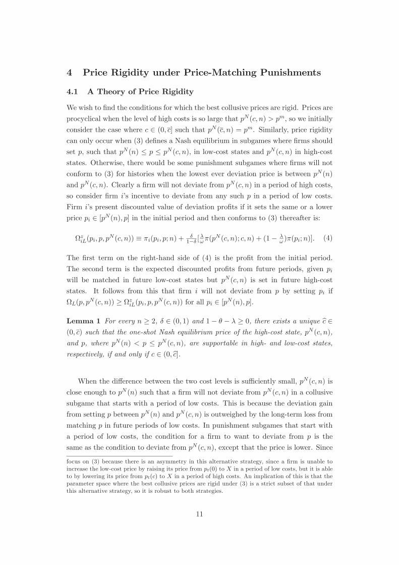
4 Price Rigidity under Price-Matching Punishments

4.1 A Theory of Price Rigidity

We wish to find the conditions for which the best collusive prices are rigid. Prices are

procyclical when the level of high costs is so large that pN (c, n) > pm, so we initially

consider the case where c ∈ (0, c] such that pN (c, n) = pm. Similarly, price rigiditycan only occur when (3) defines a Nash equilibrium in subgames where firms should

set p, such that pN (n) ≤ p ≤ pN (c, n), in low-cost states and pN (c, n) in high-coststates. Otherwise, there would be some punishment subgames where firms will not

conform to (3) for histories when the lowest ever deviation price is between pN (n)

and pN (c, n). Clearly a firm will not deviate from pN (c, n) in a period of high costs,

so consider firm i’s incentive to deviate from any such p in a period of low costs.

Firm i’s present discounted value of deviation profits if it sets the same or a lower

price pi ∈ [pN (n), p] in the initial period and then conforms to (3) thereafter is:

ΩziL(pi, p, pN (c, n)) ≡ πi(pi, p;n) +

δ1−δ [

λωπ(p

N (c, n); c, n) + (1− λω )π(pi;n)]. (4)

The first term on the right-hand side of (4) is the profit from the initial period.

The second term is the expected discounted profits from future periods, given piwill be matched in future low-cost states but pN (c, n) is set in future high-cost

states. It follows from this that firm i will not deviate from p by setting pi if

ΩL(p, pN (c, n)) ≥ ΩziL(pi, p, pN (c, n)) for all pi ∈ [pN (n), p].

Lemma 1 For every n ≥ 2, δ ∈ (0, 1) and 1− θ − λ ≥ 0, there exists a unique c ∈(0, c) such that the one-shot Nash equilibrium price of the high-cost state, pN (c, n),

and p, where pN (n) < p ≤ pN (c, n), are supportable in high- and low-cost states,

respectively, if and only if c ∈ (0, c].

When the difference between the two cost levels is sufficiently small, pN (c, n) is

close enough to pN (n) such that a firm will not deviate from pN (c, n) in a collusive

subgame that starts with a period of low costs. This is because the deviation gain

from setting p between pN (n) and pN (c, n) is outweighed by the long-term loss from

matching p in future periods of low costs. In punishment subgames that start with

a period of low costs, the condition for a firm to want to deviate from p is the

same as the condition to deviate from pN (c, n), except that the price is lower. Since

focus on (3) because there is an asymmetry in this alternative strategy, since a firm is unable toincrease the low-cost price by raising its price from pt(0) to X in a period of low costs, but it is ableto by lowering its price from pt(c) to X in a period of high costs. An implication of this is that theparameter space where the best collusive prices are rigid under (3) is a strict subset of that underthis alternative strategy, so it is robust to both strategies.

11

the standard properties of the underlying competition game imply that it is less

profitable to deviate from a price close to pN (n) than a higher price, a firm will not

deviate in any such punishment subgame, if it will not deviate from pN (c, n) in the

collusive subgame. Consequently, the punishment is credible and harsh enough to

support pN (c, n) in both cost states when the difference between the two cost levels

is sufficiently small.

In the next subsection, we limit our attention to equilibria with the same price

pc > pN (c, n) in both cost states. This allows us to characterise the best rigid price

that achieves the highest level of profit possible, given that the price does not vary

over time. In the subsection after, we find the conditions for which firms can do no

better than set the best rigid price in both cost states.

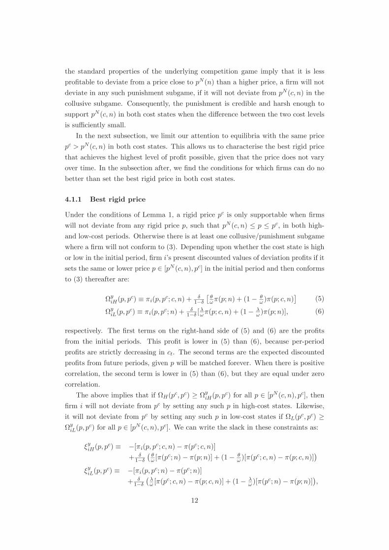
4.1.1 Best rigid price

Under the conditions of Lemma 1, a rigid price pc is only supportable when firms

will not deviate from any rigid price p, such that pN (c, n) ≤ p ≤ pc, in both high-and low-cost periods. Otherwise there is at least one collusive/punishment subgame

where a firm will not conform to (3). Depending upon whether the cost state is high

or low in the initial period, firm i’s present discounted values of deviation profits if it

sets the same or lower price p ∈ [pN (c, n), pc] in the initial period and then conformsto (3) thereafter are:

ΩyiH(p, pc) ≡ πi(p, p

c; c, n) + δ1−δ

θωπ(p;n) + (1− θ

ω )π(p; c, n) (5)

ΩyiL(p, pc) ≡ πi(p, p

c;n) + δ1−δ [

λωπ(p; c, n) + (1− λ

ω )π(p;n)], (6)

respectively. The first terms on the right-hand side of (5) and (6) are the profits

from the initial periods. This profit is lower in (5) than (6), because per-period

profits are strictly decreasing in ct. The second terms are the expected discounted

profits from future periods, given p will be matched forever. When there is positive

correlation, the second term is lower in (5) than (6), but they are equal under zero

correlation.

The above implies that if ΩH(pc, pc) ≥ ΩyiH(p, pc) for all p ∈ [pN (c, n), pc], thenfirm i will not deviate from pc by setting any such p in high-cost states. Likewise,

it will not deviate from pc by setting any such p in low-cost states if ΩL(pc, pc) ≥ΩyiL(p, p

c) for all p ∈ [pN (c, n), pc]. We can write the slack in these constraints as:

ξyiH(p, pc) ≡ −[πi(p, pc; c, n)− π(pc; c, n)]

+ δ1−δ

θω [π(p

c;n)− π(p;n)] + (1− θω )[π(p

c; c, n)− π(p; c, n)]

ξyiL(p, pc) ≡ −[πi(p, pc;n)− π(pc;n)]

+ δ1−δ

λω [π(p

c; c, n)− π(p; c, n)] + (1− λω )[π(p

c;n)− π(p;n)] ,

12

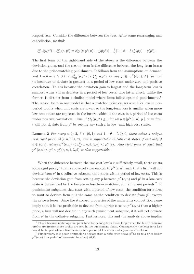
respectively. Consider the difference between the two. After some rearranging and

cancellation, we find:

ξyiH(p, pc)− ξyiL(p, p

c) = c[qi(p, pc;n)− 1

nq(pc)] + δ

ω (1− θ − λ) cn [q(p)− q(pc)].

The first term on the right-hand side of the above is the difference between the

deviation gains, and the second term is the difference between the long-term losses

due to the price-matching punishment. It follows from the assumptions on demand

and 1 − θ − λ ≥ 0 that ξyiH(p, pc) > ξyiL(p, p

c) for any p ∈ [pN (c, n), pc), so firmi’s incentive to deviate is greatest in a period of low costs under zero and positive

correlation. This is because the deviation gain is largest and the long-term loss is

smallest when a firm deviates in a period of low costs. The latter effect, unlike the

former, is distinct from a similar model where firms follow optimal punishments.6

The reason for it in our model is that a matched price causes a smaller loss in per-

period profits when unit costs are lower, so the long-term loss is smaller when more

low-cost states are expected in the future, which is the case in a period of low costs

under positive correlation. Thus, if ξyiL(p, pc) ≥ 0 for all p ∈ [pN (c, n), pc], then firm

i will not deviate from pc by setting any such p in low- and high-cost states.

Lemma 2 For every n ≥ 2, δ ∈ (0, 1) and 1 − θ − λ ≥ 0, there exists a unique

best rigid price, pyL(c, n, δ,λ, θ), that is supportable in both cost states if and only if

c ∈ (0, c], where pN (c, n) < pyL(c, n, δ,λ, θ) < pm(c). Any rigid price pc such that

pN (c, n) ≤ pc ≤ pyL(c, n, δ,λ, θ) is also supportable.

When the difference between the two cost levels is sufficiently small, there exists

some rigid price pc that is above yet close enough to pN (c, n), such that a firm will not

deviate from pc in a collusive subgame that starts with a period of low costs. This is

because the deviation gain from setting any p between pN (c, n) and pc in a low-cost

state is outweighed by the long-term loss from matching p in all future periods.7 In

punishment subgames that start with a period of low costs, the condition for a firm

to want to deviate from p is the same as the condition to deviate from pc, except

the price is lower. Since the standard properties of the underlying competition game

imply that it is less profitable to deviate from a price close to pN (c, n) than a higher

price, a firm will not deviate in any such punishment subgame, if it will not deviate

from pc in the collusive subgame. Furthermore, this and the analysis above implies

6This is because under optimal punishments the long-term loss is larger when the future collusiveprofits are greater, since profits are zero in the punishment phase. Consequently, the long-term losswould be largest when a firm deviates in a period of low costs under positive correlation.

7Furthermore, it is never profitable to deviate from a rigid price above pN (c, n) to a price belowpN (c, n) in a period of low-costs for all c ∈ (0, c].

13

that a firm will also not deviate from pc or from any rigid price between pN (c, n) and

pc in subgames that start with a period of high costs. Consequently, the punishment

is credible and harsh enough to support pc in both cost states, when pc is sufficiently

close to pN (c, n) and when the difference between the two cost levels is sufficiently

small.

The best rigid price has the unique property that a small deviation from it in

a period of low costs that is matched in all future periods balances the first-order

increase in the deviation profit with the first-order decrease in future profits (i.e.

the argument maximising (6) is pc). This implies that the (unconstrained) optimal

‘deviation’ price from the best rigid price in a period of low costs is equal to the

best rigid price. At any rigid price above this level, there is an incentive to deviate

in a period of low costs (i.e. for any pc > pyL(c, n, δ,λ, θ), then ξyiL(p, pc) < 0 for

some p < pc). Since it is less profitable to deviate in a period of high costs than

one of low costs, the (constrained) optimal ‘deviation’ price from the best rigid price

in a period of high costs also equals the best rigid price.8 The best rigid price is

equivalent to the best collusive price analysed by Lu and Wright (2010) as c → 0,

and it is strictly increasing in the level of high costs. The reason is that a given rigid

price is easier to support in a period of low costs when the high-cost level is closer

to c than when it is close to zero, because the long-term loss from a small deviation

increases with c. In contrast to Lu and Wright (2010), the monopoly price of the

low-cost state may be supportable. This is because a small deviation from pm in a

period of low costs can balance the first-order increase in the deviation profit with

the first-order decrease in future profits of high-cost states.9

4.1.2 Best collusive prices and price rigidity

The best collusive prices are rigid if a firm will deviate from any procyclical or

countercyclical prices that would be more profitable than setting the best rigid price

in both cost states. To see that such countercyclical prices are not supportable,

suppose that the initial collusive prices are p(0) and p(c) for low- and high-cost states,

respectively, where p(0) is above p(c). A necessary (but not sufficient) condition for

such prices to be more profitable than setting the best rigid price in both cost states

is that p(0) must be strictly greater than the best rigid price. Consider firm i’s

incentive to deviate in a period of low costs. Firm i’s present discounted value of8A firm would want to deviate from the best rigid price to a higher price in a period of high

costs, if firms matched such a deviation price in all future periods. However, this would not be acredible strategy even if such deviations were matched, because a firm would want to deviate fromsuch a price in punishment subgames that start with a period of low costs when the price shouldbe matched.

9There is no first-order decrease in the profits of future low-cost states, because such profitsare flat at pm. It is this feature that determines that pm is not supportable by price-matchingpunishments, when all future periods are expected to have low costs.

14

deviation profits if it sets the same or a lower price p ∈ [p(c), p(0)] in the initialperiod, then conforms to (3) thereafter is:

ΩxiL(p, p(0), p(c)) ≡ πi(p, p(0);n) +δ1−δ [

λωπ(p(c); c, n) + (1− λ

ω )π(p;n)].

Thus, a firm will not deviate from p(0) by setting p if ΩL(p(0), p(c)) ≥ ΩxiL(p, p(0), p(c))for all p ∈ [p(c), p(0)], where the slack in this constraint is:

ξxiL(p, p(0)) ≡ −[πi(p, p(0);n)− π(p(0);n)] + δ1−δ (1− λ

ω )[π(p(0);n)− π(p;n))].

Notice that ξxiL(p, p(0)) does not depend on p(c), because the punishment results in

firms still setting p(c) in high-cost states, and as a consequence it is the same as

ξyiL(p, p(0)), except that there is no long-term loss in profits of future high-cost states.

This implies that since it is profitable for a firm to deviate from a rigid price above the

best rigid price in a period of low costs, then an otherwise identical deviation is even

more profitable when prices are countercyclical (i.e. for any p(0) > pyL(c, n, δ,λ, θ),

ξxiL(p, p(0)) < ξyiL(p, p(0)) < 0 for some p < p(0)). Therefore, the best collusive

prices cannot be countercyclical.

Now consider whether the best collusive prices can be procyclical, where p(c)

is above p(0). First consider how this affects the best collusive price of the low-

cost state, denoted p∗(0) ∈ [pN (c, n), pm]. Notice that firm i’s present discounted

value of deviation profits is equivalent to (6), if it deviates from p(0) to some p ∈[pN (c, n), p(0)] in a period of low costs. Thus, such a deviation is not profitable

if ΩL(p(0), p(c)) ≥ ΩyiL(p, p(0)) for all p ∈ [pN (c, n), p(0)]. Since ΩL(p(0), p(c))

increases with p(c) but ΩyiL(p, p(0)) is independent of p(c), then there is still no

incentive to deviate from the best rigid price when prices are procyclical. However,

a price above the best rigid price is not supportable in low-cost states, because the

punishment for such a price is not credible. This is because for any such price there

are some punishment subgames where firms should match a price above the best

rigid price in all future periods, but each firm has an incentive to deviate from it

in such punishment subgames that start with a period of low costs. Consequently,

the best rigid price is the highest price that is supportable in low-cost states when

prices are rigid or procyclical. However, it is more profitable to set the monopoly

price when the best rigid price is above it, so p∗(0) is the lower of the best rigidprice and the monopoly price of the low-cost state for all c ∈ (0, c].

Finally, to find whether procyclical prices are supportable, consider firm i’s in-

centive to deviate from p(c) above p∗(0) in a period of high costs, while holding thecollusive price of low-cost states fixed at p∗(0). Firm i’s present discounted value

of deviation profits if it sets the same or a lower price p ∈ [p∗(0), p(c)] in the initial

15

period, then conforms to (3) thereafter is:

ΩxiH(p, p(c), p∗(0)) ≡ πi(p, p(c); c, n) +

δ1−δ

θωπ(p

∗(0);n) + (1− θω )π(p; c, n) .

(7)

The first term on the right-hand side of (7) is the profit from the initial period.

The second term represents the expected discounted profits from future periods,

given p will be matched in future high-cost states but p∗(0) is set in future low-cost states. It follows from this that firm i will not deviate from p(c) by setting

p if ΩH(p(c), p∗(0)) ≥ ΩxiH(p, p(c), p∗(0)) for all p ∈ [p∗(0), p(c)]. The slack in this

constraint is:

ξxiH(p, p(c)) ≡ −[πi(p, p(c); c, n)− π(p(c); c, n)] + δ1−δ (1− θ

ω )[π(p(c); c, n)− π(p; c, n))],

which does not depend on p∗(0) because the punishment results in firms still settingp∗(0) in low-cost states.

To see that the best collusive prices can be rigid under price-matching punish-

ments, suppose firm i deviates from p(c) to p = p∗(0). Given the punishment islimited to future high-cost states when such a deviation is matched, there is no

long-term loss for such a deviation when all future periods are expected to have low

costs (i.e. θ = 1 and λ = 0). Thus, each firm will have an incentive to deviate from

any p(c) above p∗(0), and the best collusive prices are rigid at p∗(0) for all c ∈ (0, c].Proposition 1 shows that the best collusive prices can still be rigid when high costs

persist into the future.

Proposition 1 For every n ≥ 2, δ ∈ (0, 1) and 1− θ− λ ≥ 0, there exists a uniquec∗ ∈ (0, c) such that the best rigid price, pyL(c, n, δ,λ, θ), is the best collusive price inboth cost states if and only if c ∈ (0, c∗], where pN (c, n) < pyL(c, n, δ,λ, θ) < pm.

When the difference between the two cost levels is below the critical threshold, a

firm will want to deviate from a price above yet very close to the best rigid price in

high-cost states. To see this point, consider a deviation from such a p(c) to a price

equal to or just above p∗(0) in a period of high costs.10 Notice that ξxiH(p, p(c)) is

the same as ξyiL(p, p(c)) as c→ 0, except that there is no long-term loss in profits of

future low-cost states. This implies that since it is profitable to deviate from a rigid

price above the best rigid price in a period of low costs, then an otherwise identical

deviation is even more profitable in a period of high costs as c → 0 when prices

are procyclical (i.e. for any p(c) > pyL(c, n, δ,λ, θ), ξxiH(p, p(c)) < ξyiL(p, p(c)) < 0

for some p < p(c) as c → 0). As the level of high costs increases towards c∗, the10 It is never profitable to deviate from any procyclical p(c) by setting a price below p∗(0) in a

period of high costs for all c ∈ (0, c].

16

profitability of such a deviation falls.11 However, a price above yet very close to the

best rigid price is not supportable until the level of high costs exceeds c∗.Prices above yet very close to the best rigid price may not be supportable in high-

cost states, even though the best rigid price is always supportable. This is because

there is a discontinuity in the incentives to collude at p∗(0), which arises due to thefact that a deviation from p(c) to a price that is equal to or just above p∗(0) onlylowers prices in future high-cost states. Consequently, such a deviation from a price

above yet very close to the rigid price in a period of high costs generates a much

smaller long-term loss than an otherwise identical deviation from the rigid price,

where price matching reduces the prices of all future periods. Yet, the deviation

gains are effectively the same for such deviations. As a result, for some positive

values of c, it can be the case that a deviation from a price above yet very close

to the best rigid price is strictly profitable in a period of high costs, even though a

deviation from the best rigid price is strictly unprofitable.

When the difference between the two cost levels is so large that the best collusive

price of the low-cost state is pm, the best collusive prices are procyclical. This is

because pm is the best collusive price of low-cost states, if the first-order increase

in the deviation profit from a small deviation from pm in a period of low costs is

outweighed by the first-order decrease in profits of future high-cost states (there is

no first-order decrease in profits of future low-cost states, since such profits are flat

at pm). In comparison to this, a small deviation from a price above yet very close to

pm in a period of high costs leads to a smaller first-order increase in the deviation

profits and a (weakly) larger first-order decrease in profits of future high-cost states.

This implies that the best collusive prices will be procyclical, because a firm will not

deviate from a price above yet very close to pm in a period of high costs, if a firm

will not deviate from pm in a period of low costs.

4.2 Price rigidity and the expected duration of a high-cost phase

The best collusive prices are rigid when the difference between the two costs levels

is below the critical threshold. Proposition 2 now shows that this critical threshold

depends upon the extent to which a high-cost state is likely to persist into the

future. To see this point, define a high-cost phase as a sequence of high-cost states

that begins in a period where costs change from the low- to the high-cost state and

ends the period before they change back. The expected duration of a high-cost phase

is Σ∞t=1tθ(1 − θ)t−1 = 1/θ, which implies that the lower the probability that costs

11This is because the deviation gain strictly decreases and long-term loss strictly increases as thelevel of high costs rises, due to the fact that high-cost states are less profitable than before; andit is despite of the fact that the deviation occurs from a slightly higher price, since the best rigidprice strictly increases with the level of high costs.

17

will change from the high- to the low-cost state in the following period, the longer

a high-cost phase is likely to last. Similarly, we can define a low-cost phase with an

expected duration of 1/λ.

Proposition 2 For every n ≥ 2, δ ∈ (0, 1) and 1− θ− λ ≥ 0, the critical differencebetween the two cost levels, c∗, is strictly decreasing in the expected duration of ahigh-cost phase.

As the expected duration of a high-cost phase increases, other things equal, it

is easier to support a price above yet very close to the best rigid price in high-cost

states. This comes about from two opposing effects. First, a direct effect reduces

the profitability of a small deviation from such a price. Second, an indirect effect

raises the profitability of such a deviation, because the deviation occurs from a

slightly higher price than before, since the best rigid price strictly increases with the

expected duration of a high-cost phase. Both effects are caused by the fact that the

punishment strategy leads to larger long-term losses when future periods are likely

to consist of more high-cost states. The direct effect dominates the indirect effect,

which implies that, for a given difference between the two cost levels, procyclical

prices are easier to support as the expected duration of a high-cost phase increases,

so the critical threshold falls. When there is zero correlation (so that the expected

duration of a low-cost phase decreases at the same rate as the expected duration

of a high-cost phase increases) both the direct and indirect effects are larger than

under positive correlation, but the direct effect still dominates.

We have already seen that the best collusive prices are rigid when a high-cost

phase is expected to last only one period and the following low-cost phase lasts

forever, provided the one-shot Nash equilibrium price of the high-cost state is not

above the best rigid price (i.e. c∗ → c as θ → 1 and λ→ 0). On the other hand, when

a high-cost phase is expected to last forever, the best collusive prices are procyclical,

regardless of the expected duration of a low-cost phase (i.e. c∗ → 0 as θ → 0 for all

0 < λ < 1). This is because for such conditions it is more profitable to deviate from

a rigid price in a period of low costs than to deviate from a price above yet very

close to the rigid price in a period of high costs (i.e. as θ → 0, ξxiH(p, pc) > ξyiL(p, p

c)

for all p < pc). Therefore, provided a firm will not deviate from the rigid price in

low-cost states, it will not deviate from a price above yet very close to the rigid price

in high-cost states.

4.3 Price rigidity and profits over the fluctuations

The preceding analysis showed that the best rigid price strictly increases with the

level of high costs. Proposition 3 shows that this implies that there are also general

18

properties for the resultant collusive profits when the best collusive prices are rigid.

Proposition 3 For any c ∈ (0, c∗), per-period profits when costs are high (low) arestrictly decreasing (increasing) in the level of high costs, c, when firms set the best

rigid price. The present discounted values of collusive profits are strictly decreasing

in c when firms set the best rigid price in both states, whether the initial period has

high or low costs.

Clearly, per-period profits are greater in a low-cost state than in a high-cost

state, when firms set the best rigid price in both states. As the level of high costs

rises towards c∗, the difference in such profits becomes larger for two reasons. First,per-period profits in low-cost states are larger than before, since the best rigid price

rises with the level of high cost but it remains below pm. Second, per-period profits

in high-cost states are smaller than before, because the best rigid price rises with

the level of high costs at a rate that is less than one-to-one. In contrast, the present

discounted values of collusive profits are equal when the high-cost level is equal to the

low-cost level, but such profits fall as the high-cost level rises towards c∗, regardlessof whether the initial period has low or high costs.

5 An Example

We complement the above analysis by assuming that demand is derived from the con-

stant elasticity of substitution version of Spence-Dixit-Stiglitz preferences (Spence,

1976; and Dixit and Stiglitz, 1977). We do this for three reasons. First, we want to

show that the best collusive prices are rigid for reasonably large differences in the

two cost levels. Second, we want to investigate the effect of the degree of product

differentiation on such price rigidity. To the author’s knowledge, there is no other

model of collusive price rigidity that considers this, since both Athey et al (2004)

and Hanazono and Yang (2007) analyse homogeneous products. Third, we want to

investigate the effect of the number of firms in the market on such price rigidity,

and this ultimately depends upon the degree of product differentiation. We use

Spence-Dixit-Stiglitz preferences, because it falls into the class of our general model

and it generates results with simpler intuition than alternatives, since it isolates

the competitive effects of product differentiation as there is no market expansion

effect.12

12Spence-Dixit-Stiglitz preferences is one example of differentiated demand analysed by Kühnand Rimler (2007) for collusion models under Nash reversion and optimal punishment strategies.It has not been analysed for collusion under price-matching punishments before. Similar resultsas those presented here can be derived using the standard Bertrand competition model with lineardemands.

19

A representative consumer’s utility function is U(x) = n1−κ1−κ

1nΣx

1−φκi

1−κ1−φκ

+m,

where x is the vector of consumption of the n products, m is expenditure on other

goods, φ ∈ (0, 1) measures the degree of product differentiation, where products areless differentiated the closer φ is to zero, and κ ∈ (0, 1) is a parameter. It followsfrom this utility function that the direct demand function for firm i is:

qi(pi,p−i,φ, n) =1

np− 1κ

i

n

Σj (pi/pj)1−φκφκ

1−φ1−φκ

.

This implies that total demand at equal prices is independent of both the degree of

product differentiation and the number of firms, i.e. q(p) = p−1/κ. It is straightfor-ward to show that the monopoly price is pm(ct) = ct/(1− κ) and that the one-shot

Nash equilibrium price is pN (ct, n,φ) = ct/ 1− κ/ 1 + 1−φφ

n−1n . To ensure that

the monopoly price is above the one-shot Nash equilibrium price for both cost states,

we assume that the level of low costs is c ∈ (0, c) and we normalise the high-costlevel relative to the low-cost level later.

For this example, the best rigid price is:

pyL(c, n, δ,λ, θ,φ) =c

1−κ/ 1+(1−δ) 1−φφ

n−1n

+ δλ(c−c)ω 1−κ+(1−δ) 1−φ

φn−1n

, (8)

which applies for c < c ≤ c.13 The first term on the right hand-side of (8) is

equivalent to the best collusive price analysed in Lu and Wright (2010) and the

second term captures the effect of varying costs. This price equals c when products

are homogeneous, and it is everywhere strictly increasing in the degree of product

differentiation, φ. It is above the one-shot Nash equilibrium price of the low-cost

state for all 0 < φ ≤ 1, and it is above the monopoly price of the low-cost state whenproducts are not substitutable. It is everywhere strictly decreasing in the number of

firms, n, but it is always above the one-shot Nash equilibrium price of the low-cost

state, even when there is a large number of firms in the market.14

The price in (8) defines the best collusive price in both cost states when the

difference between the two cost states is below the critical threshold. It follows from

Proposition 1 that c∗ = c1−K ∈ (c, c) where:

K ≡ κ δθω(1−δ) 1−φ

φn−1n

(1−κ)(1− δθω)+(1−δ) 1−φ

φn−1n

1− δλω+(1−δ) 1−φ

φn−1n

∈ (0, 1).

13Following Lemma 1, c = 1− κ/ 1 + 1−φφ

n−1n

c

1−κ(1− δλω)/ (1−δ) 1+ 1−φ

φn−1n

+δ(1− λω).

14This is because the underlying competition game is one of true monopolistic competition, wherethe price is above marginal cost even as n→∞.

20

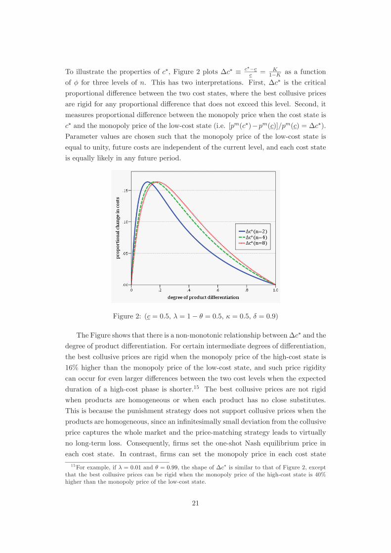
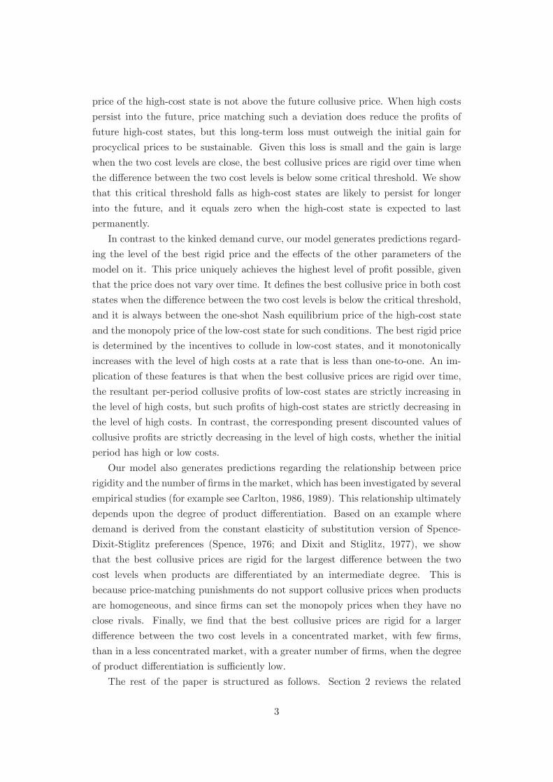
To illustrate the properties of c∗, Figure 2 plots Δc∗ ≡ c∗−cc = K

1−K as a function

of φ for three levels of n. This has two interpretations. First, Δc∗ is the criticalproportional difference between the two cost states, where the best collusive prices

are rigid for any proportional difference that does not exceed this level. Second, it

measures proportional difference between the monopoly price when the cost state is

c∗ and the monopoly price of the low-cost state (i.e. [pm(c∗)−pm(c)]/pm(c) = Δc∗).Parameter values are chosen such that the monopoly price of the low-cost state is

equal to unity, future costs are independent of the current level, and each cost state

is equally likely in any future period.

Figure 2: (c = 0.5, λ = 1− θ = 0.5, κ = 0.5, δ = 0.9)

The Figure shows that there is a non-monotonic relationship betweenΔc∗ and thedegree of product differentiation. For certain intermediate degrees of differentiation,

the best collusive prices are rigid when the monopoly price of the high-cost state is

16% higher than the monopoly price of the low-cost state, and such price rigidity

can occur for even larger differences between the two cost levels when the expected

duration of a high-cost phase is shorter.15 The best collusive prices are not rigid

when products are homogeneous or when each product has no close substitutes.

This is because the punishment strategy does not support collusive prices when the

products are homogeneous, since an infinitesimally small deviation from the collusive

price captures the whole market and the price-matching strategy leads to virtually

no long-term loss. Consequently, firms set the one-shot Nash equilibrium price in

each cost state. In contrast, firms can set the monopoly price in each cost state

15For example, if λ = 0.01 and θ = 0.99, the shape of Δc∗ is similar to that of Figure 2, exceptthat the best collusive prices can be rigid when the monopoly price of the high-cost state is 40%higher than the monopoly price of the low-cost state.

21

when they are local monopolies, with no close substitutes.

Finally, Figure 2 shows that Δc∗ is larger for concentrated markets, with fewfirms, than for less concentrated markets, with a greater number of firms, when the

degree of product differentiation is sufficiently low; the opposite relationship may

exist otherwise. This is not inconsistent with empirical research that shows that

prices are less responsive to changes in market conditions in some cases when the

markets are more concentrated (see Dixon, 1983; Carlton, 1986; Bedrossian and

Moschos, 1988; Geroski, 1992; Weiss, 1995) but the opposite relationship exists in

others (see Domberger, 1979; and Kardasz and Stollery, 1988). The reason behind

this result in our model is that it can either be more or less profitable to deviate

from a price above yet very close to the best rigid price in a period of high costs,

as the number of firms increases. This is because there are two opposing effects.

First, a direct effect raises the profitability of a small deviation from such a price.

Second, an indirect effect reduces the profitability of such a deviation, because the

deviation occurs from a slightly lower price than before, since the best rigid price

strictly decreases with the number of firms in the market. Both effects are caused

by the fact that the deviation gains are larger and the punishment strategy leads to

smaller long-term losses when there are a greater number of firms in the market (from

Assumption 4 and symmetric demand, respectively). In our general framework, it

is not possible to sign the overall effect. In our example, however, the indirect effect

dominates the direct effect when the degree of product differentiation is sufficiently

low. This implies that, for a given difference between the two cost levels, procyclical

prices are easier to support as the number of firms in the market increases, so the

critical threshold falls.

6 Concluding remarks

In this paper, we analysed an infinitely repeated game where unit costs alternate

stochastically between low and high states and where firms employ a price-matching

punishment strategy. This provided game theoretic support for the results of the

kinked demand curve, because we showed that the best collusive prices can be rigid

over time when the difference between the two costs levels is below some critical

threshold. Moreover, we showed that this critical threshold is closer to zero as

high-cost states are likely to persist for longer into the future, and it equals zero

when the high-cost state is expected to last permanently. When the best collusive

prices are rigid over time, the best rigid price is always between the one-shot Nash

equilibrium price of the high-cost state and the monopoly price of the low-cost state,

and it monotonically increases with the level of high costs at a rate that is less than

one-to-one. As a result, an increase in the level of high costs raises the resultant per-

22

period profits of a low-cost state, but it reduces such per-period profits of a high-cost

state. Nevertheless, the corresponding present discounted values of collusive profits

are decreasing in the level of high costs, whether the initial period has high or low

costs. Finally, when demand is derived from the constant elasticity of substitution

version of Spence-Dixit-Stiglitz preferences, we found that the best collusive prices

are rigid for the largest difference between the two cost levels when products are

differentiated by an intermediate degree; and that the best collusive prices are rigid

for a larger difference between the two cost levels in a concentrated market than in

a less concentrated market, when the degree of product differentiation is sufficiently

low.

Throughout the paper, we have considered only two cost states, but periods of

price rigidity are not restricted to this special case. For example, when a medium-

cost state is added and there is zero correlation, the best rigid price is unaffected by

the introduction of the third state, if the expected level of future costs is unchanged

compared to the two-state model. Moreover, holding the expected level of future

costs constant also ensures that future high-cost states are less likely in this three-

state model than the two-state model. As a result, there is a greater incentive to

deviate from a procyclical price in a period of high costs in this three-state model

than the two-state model, when such a deviation only leads to a long-term loss in

profits of future high-cost states. Thus, when the difference between the low- and the

high-cost states is such that the best collusive prices are rigid in the two-state model,

the best collusive prices in this three-state model will either be rigid for every cost

state or partially rigid (where the best collusive prices are rigid in medium- and high-

cost states, at a price above the best collusive price of low-cost states). Applying

this logic to more than three cost states suggests that it is even more difficult to

support procyclical prices in the highest-cost state than in the two-state model, so

periods of price rigidity can occur for any number of states.

Finally, an important avenue for future research is to investigate whether there

exists any circumstances where firms will choose to support collusive prices through a

weaker punishment, such as price matching, rather than harsher punishment strate-

gies, such as Nash reversion or optimal punishment strategies. Such a theoretical

justification for price matching may provide a better indication of the industry char-

acteristics where price rigidity is likely to prevail. It would also resolve the tension

between the informal reasoning behind the belief that firms will employ the harsh-

est credible punishment with the evidence that, at least in some situations, tacitly

colluding firms (and even some cartels) do not employ such punishments.

23

References

[1] Abreu, D (1986) “Extremal Equilibria of Oligopolistic Supergames,” Journal ofEconomic Theory, 39, 191-225

[2] Abreu, D (1988) “On the Theory of Infinitely Repeated Games with Discount-ing,” Econometrica, 56, 383-396

[3] Athey, S, Bagwell, K and Sanchirico, C (2004) “Collusion and Price Rigidity,”Review of Economic Studies, 71(2), 317-349

[4] Bagwell, K and Staiger, R (1997) “Collusion over the Business Cycle,” RANDJournal of Economics, 28(1), 82-106

[5] Bedrossian, A and Moschos, D (1988) “Industrial Structure, Concentration andthe Speed of Price Adjustments,” Journal of Industrial Economics, 36, 459-475

[6] Bhaskar, V (1988) “The Kinked Demand Curve: A Game Theoretic Approach,”International Journal of Industrial Organization, 6, 373-384

[7] Carlton, D (1986) “The Rigidity of Prices,” American Economic Review, 76(4),637-658

[8] Carlton, D (1989) “The Theory and the Facts of How Markets Clear: IsIndustrial Organization Valuable for Understanding Macroeconomics?” inSchmalensee, R and Willig, R (eds) Handbook of Industrial Organization, Ox-ford: North-Holland

[9] Dixit, A and Stiglitz, J (1977) “Monopolistic Competition and Optimum Prod-uct Diversity,” American Economic Review, 67, 63-78

[10] Dixon, R (1983) “Industry Structure and the Speed of Price Adjustments,”Journal of Industrial Economics, 31, 25-37

[11] Domberger, S (1979) “Price Adjustment and Market Structure,” EconomicJournal, 89, 96-108

[12] Friedman, J (1971) “A Non-Cooperative Equilibrium for Supergames,” Reviewof Economic Studies, 28, 1-12

[13] Fudenberg, D and Tirole, J (1991) Game Theory, Cambridge: MIT Press

[14] Genesove, D and Mullin, M. (2001) “Rules, Communication, and Collusion:Narrative Evidence from the Sugar Institute Case,” American Economic Re-view, 91, 379-398

[15] Geroski, P (1992) “Price Dynamics in UK Manufacturing: A MicroeconomicView,” Economica, 59, 403-19

[16] Green, E and Porter, R (1984) “Non-cooperative Collusion under ImperfectPrice Information,” Econometrica, 52, 87-100

24

[17] Hall, R and Hitch, C (1939) “Price Theory and Business Behaviour,” OxfordEconomic Papers, 2, 12-45

[18] Haltiwanger, J and Harrington, J (1991) “The Impact of Cyclical DemandMovements on Collusive Behavior,” RAND Journal of Economics, 22(1), 89-106

[19] Hanazono, M and Yang, H (2007) “Collusion, Fluctuating Demand, and PriceRigidity,” International Economic Review, 48(2) 483-515

[20] Kalai, E and Satterthwaite, M (1994) “The Kinked Demand Curve, Facilitat-ing Practices, and Oligopolistic Coordination,” in Gilles, R and Ruys, P (eds)Imperfections and Behavior in Economic Organizations, Kluwer Academic Pub-lishers

[21] Kardasz, S and Stollery, K (1988) “Market Structure and Price Adjustment inCanadian Manufacturing Industries,” Journal of Economics and Business, 40,335-342

[22] Kühn K-U and Rimler, M (2007) “The Comparative Statics of Collusion Mod-els,” mimeo, University of Michigan

[23] Levenstein, M. (1997) “Price Wars and the Stability of Collusion: A Study ofthe Pre-World War I Bromine Industry,” Journal of Industrial Economics, 45,117-136

[24] Lu, Y and Wright, J (2010) “Tacit Collusion with Price-Matching Punish-ments,” International Journal of Industrial Organization, 28, 298-306

[25] Maskin, E and Tirole, J (1988) “A Theory of Dynamic Oligopoly II: PriceCompetition, Kinked Demand Curves and Edgeworth Cycles,” Econometrica,56(3), 571-599

[26] Rotemberg, J and Saloner, G (1986) “A Supergame-Theoretic Model of PriceWars during Booms,” American Economic Review, 76, 390-407

[27] Slade, M (1987) “Interfirm Rivalry in a Repeated Game: An Empirical Test ofTacit Collusion,” Journal of Industrial Economics, 35, 499-516

[28] Slade, M (1989) “Price Wars in Price Setting Supergames,” Economica, 223,295-310

[29] Slade, M (1990) “Strategic Pricing Models and Interpretation of Price WarData,” European Economic Review, 34, 524-537

[30] Slade, M (1992) “Vancouver’s Gasoline Price Wars: An Empirical Exercise inUncovering Supergame Strategies,” Review of Economic Studies, 59, 257-276

[31] Spence, M (1976) “Product Differentiation and Welfare,” American EconomicReview, 66, 407-414

[32] Sweezy, P (1939) “Demand Under Conditions of Oligopoly,” Journal of PoliticalEconomy, 47, 568-573

25

[33] Tirole, J (1988) Theory of Industrial Organization, Cambridge: MIT Press

[34] Vives, X (2001) Oligopoly Pricing: Old Ideas and New Tools, Cambridge: MITPress

[35] Weiss, C (1995) “Determinants of Price Flexibility in Oligopolistic Markets:Evidence from Austrian Manufacturing,” Journal of Economics & Business,47, 423-439

A Proofs

Proof of Lemma 1. Suppose the collusive price is pN (c, n) in both cost states.

To prove subgame perfection, it suffices to check that there is no history that leads

to a subgame in which a one-stage deviation is profitable. For every history, the

lowest ever deviation price below pN (c, n) at some period τ is min{pdτ , pN (c, n)}. Ifmin{pdτ} ≤ pN (n), then (3) trivially defines a Nash equilibrium in the subsequent

punishment subgames, whether they start with a period of high or low costs. Other-

wise, the subsequent punishment subgames are identical to a history in which firms

had set pN (c, n) in high-cost states and min{pdτ , pN (c, n)} ∈ (pN (n), pN (c, n)] in

low-cost states. Clearly, (3) defines a Nash equilibrium in the subgames that start

with a period of high costs. Thus, we must find the conditions for which a firm will

not deviate from pN (c, n) or from any price between pN (n) and pN (c, n) in subgames

that start with a period of low costs.

Suppose we consider some collusive price p ∈ (pN (n), pN (c, n)] that is set in

low-cost states, where pN (c, n) is set in high-cost states. Consider firm i setting the

same or a lower price pi ∈ [pN (n), p] in a period of low costs. From (4) define:

ΔΩzL(p) ≡ ∂πi(pi,p;n)∂pi

+ δ1−δ (1− λ

ω )dπ(pi;n)dpi pi=p

.

Firm i will not deviate from p ifΔΩzL(p) ≥ 0, otherwise ΩL(p, pN (c, n)) < ΩziL(pi, p, pN (c, n))for some pi < p. We wish to show that if ΔΩzL(p

N (c, n)) ≥ 0, then ΔΩzL(p) ≥ 0 ∀p ∈ (pN (n), pN (c, n)). Differentiating ΔΩzL(p) with respect to p yields:

d(ΔΩzL(p))dp = ∂2πi(pi,p;n)

∂p2i+ j=i

∂2πi(pi,p;n)∂pi∂pj

+ δ1−δ (1− λ

ω )d2π(pi;n)dp2i pi=pj=p

.

It follows from (2) and Assumption 5 that d(ΔΩzL(p))dp < 0. Hence, if ΔΩzL(p

N (c, n)) ≥0, then ΔΩzL(p) > 0 ∀ p ∈ (pN (n), pN (c, n)). Thus, a firm will not deviate from a

price between pN (n) and pN (c, n), if it will not deviate from pN (c, n).

There exists a unique c ∈ (0, c) such thatΔΩzL(pN (c, n)) = 0 becauseΔΩzL(pN (n)) >

26

0, ΔΩzL(pN (c, n)) = ΔΩzL(p

m) < 0 and:

d(ΔΩzL(pN ))

dc =d(ΔΩzL(p))

dpdpN

dc p=pN (c,n)< 0,

since d(ΔΩzL(p))dp < 0 and dpN

dc > 0. Thus, ΔΩzL(pN (c, n)) ≥ 0 if and only if c ∈ (0, c].

The above analysis implies that pN (c, n) and p, such that pN (n) < p ≤ pN (c, n), aresupportable in high- and low-cost states, respectively, if and only if c ∈ (0, c].

Proof of Lemma 2. Suppose the collusive price is pc in both cost states. To prove

subgame perfection, it suffices to check that there is no history that leads to a sub-

game in which a one-stage deviation is profitable. For every history, the lowest ever

deviation price below pc at some period τ is min{pdτ , pc}. If min{pdτ , pc} ≤ pN (c, n),then (3) defines a Nash equilibrium in the subsequent punishment subgames, whether

they start with a period of high or low costs, if and only if c ∈ (0, c] (from Lemma

1). Otherwise, the subsequent punishment subgames are identical to a history in

which firms had set min{pdτ , pc} ∈ (pN (c, n), pc] in both high- and low-cost states.Thus, we must find the conditions for which a firm will not deviate from pc or from

any rigid price between pN (c, n) and pc in subgames that start with a period of high

or low costs.

Suppose we consider some collusive price p ∈ (pN (c, n), pc] that is set in bothcost states, where c ∈ (0, c]. First, consider firm i setting a lower price pi ∈[pN (n), pN (c, n)] in a period of low costs, so its present discounted value of devi-

ation profits are given by (4). It is more profitable to deviate from p to pN (c, n)

than to any price below pN (c, n), because ΔΩzL(pN (c, n)) ≥ 0 ∀ c ∈ (0, c] and prices

are strategic complements. Thus, we must consider deviations where firm i sets the

same or a lower price pi ∈ [pN (c, n), p]. From (5) and (6), respectively, define:

ΔΩyH(p) ≡ ∂πi(pi,p;c,n)∂pi

+ δ1−δ

θωdπ(pi;n)dpi

+ [1− θω ]dπ(pi;c,n)

dpi pi=p

ΔΩyL(p) ≡ ∂πi(pi,p;n)∂pi

+ δ1−δ

λωdπ(pi;c,n)

dpi+ [1− λ

ω ]dπ(pi;n)dpi pi=p

.

Firm i will not deviate from p in a period of low costs if ΔΩyL(p) ≥ 0, otherwise

ξyiL(pi, p) < 0 for some pi < p. We wish to show that if ΔΩyL(p

c) ≥ 0, then ΔΩyL(p) ≥0 and ΔΩyH(p) ≥ 0 ∀ p ∈ (pN (c, n), pc]. First, differentiating ΔΩyL(p) with respectto p yields:

d(ΔΩyL(p))dp = ∂2πi(pi,p;n)

∂p2i+ j=i

∂2πi(pi,p;n)∂pi∂pj

+ δ1−δ

λωd2π(pi;c,n)

dp2i+ [1− λ

ω ]d2π(pi;n)dp2i pi=pj=p

.

It follows from (2) and Assumption 5 that d(ΔΩyL(p))dp < 0. Hence, if ΔΩyL(p

c) ≥ 0,

then ΔΩyL(p) > 0 ∀ p ∈ (pN (c, n), pc). Thus, if firm i will not deviate from pc in a

27

period of low costs, then it will not deviate from a lower rigid price between pN (c, n)

and pc. Next, consider:

ΔΩyH(p)−ΔΩyL(p) = − c∂qi(pi,p;n)∂pi+ δ

ω (1− θ − λ) cndq(pi)dpi pi=p

.

Assumption 1 and 1−θ−λ ≥ 0 imply that the above is positive. So, if ΔΩyL(pc) ≥ 0,then ΔΩyH(p) > ΔΩ

yL(p) ≥ 0 ∀ p ∈ (pN (c, n), pc]. Thus, firm i will also not deviate

from pc or any rigid price between pN (c, n) and pc in a period of high costs.

Given d(ΔΩyL(p))dp < 0, there exists a unique best rigid price, pyL(c, n, δ,λ, θ), which

is the level of p that solves ΔΩyL(p) = 0. It satisfies pN (c, n) < pyL(c, n, δ,λ, θ) <

pm(c) since ΔΩyL(pN (c, n)) > ΔΩzL(p

N (c, n)) ≥ 0 ∀ c ∈ (0, c] and ΔΩyL(pm(c)) <0. The above analysis implies that any rigid price pc such that pN (c, n) < pc ≤pyL(c, n, δ,λ, θ) is supportable if and only if c ∈ (0, c].

Proof of Proposition 1. Suppose the collusive prices are p(0) and p(c) >

p(0) in low- and high-cost states, respectively, where without loss of generality let

p(0) > pN (c, n). To prove subgame perfection, it suffices to check that there is

no history that leads to a subgame in which a one-stage deviation is profitable.

For every history, the lowest ever deviation price below p(cτ ) at some period τ is

min{pdτ , p(cτ )}. If min{pdτ} ≤ pN (c, n) < p(0), then (3) defines a Nash equilibriumin the subsequent punishment subgames, whether they start with a period of high

or low costs, if and only if c ∈ (0, c] (from Lemma 1). If pN (c, n) < min{pdτ} ≤ p(0),then (3) defines a Nash equilibrium in the subsequent punishment subgames, whether

they start with a period of high or low costs, if and only if p(0) ≤ pyL(c, n, δ,λ, θ)

(from Lemma 2). Otherwise, the subsequent punishment subgames are identical to

a history in which firms had set min{pdτ , p(c)} ∈ (p(0), p(c)] in high-cost states andp(0) in low-cost states. Thus, to find when procyclical prices are supportable, we

must find the conditions for which a firm will not deviate from p(c) or from any

price between p(0) and p(c) in subgames that start with a period of high costs.

Moreover, we have to check that a firm will not deviate from p(0) ≤ pyL(c, n, δ,λ, θ)when p(c) > p(0) in subgames that start with a period of low costs.

Suppose we consider some collusive prices such that p(0) > pN (c, n) is set in

low-cost states and p ∈ (p(0), p(c)] is set in high-cost states, where c ∈ (0, c].

Furthermore, recall that there are punishment subgames in which a firm will not

conform to (3) for any p(0) above pyL(c, n, δ,λ, θ), so it must be the case that

p(0) ≤ pyL(c, n, δ,λ, θ). Consider firm i deviating from such a p(0) in a period of

low costs. It is not profitable to set a higher price, because this decreases profits

in the initial period and it decreases profits of future high-cost states. Moreover, it

is not profitable to deviate to pi ∈ [pN (c, n), p(0)], because given ΩL(p(0), p(0)) ≥

28

ΩyiL(pi, p(0)) ∀ pi ∈ [pN (c, n), p(0)] if p(0) ≤ pyL(c, n, δ,λ, θ) (from Lemma 2), then

ΩL(p(0), p) > ΩyiL(pi, p(0)) for any such pi. Finally, it is not profitable to set

pi ∈ [pN (n), pN (c, n)) because it is more profitable to deviate from p(0) to pN (c, n)

than to any price below pN (c, n), since ΔΩzL(pN (c, n)) ≥ 0 ∀ c ∈ (0, c] and prices

are strategic complements. This implies that a firm will not deviate from any p(0),

such that pN (c, n) < p(0) ≤ pyL(c, n, δ,λ, θ), when p > p(0). Thus, the best collusiveprice of the low-cost state is p∗(0) = min{pyL(c, n, δ,λ, θ), pm} ∀ c ∈ (0, c].

Now suppose the collusive prices are p ∈ (p∗(0), p(c)] in high-cost states andp∗(0) in low-cost states, where c ∈ (0, c]. First, consider firm i setting a lower price

pi ∈ [pN (c, n), p∗(0)], so its present discounted value of deviation profits are givenby (5). It is more profitable to deviate from p to p∗(0) than to a price below p∗(0)in a period of high costs, because ΔΩyH(p

∗(0)) > ΔΩyL(p∗(0)) ≥ 0 ∀ c ∈ (0, c] and

prices are strategic complements. Thus, we must consider deviations where firm i

sets the same or a lower price pi ∈ [p∗(0), p]. From (7), define:

ΔΩxH(p) ≡ ∂πi(pi,p;c,n)∂pi

+ δ1−δ (1− θ

ω )dπ(pi;c,n)

dpi pi=p.

Firm i will not deviate from p if ΔΩxH(p) ≥ 0, otherwise ξxiH(pi, p) < 0 for some

pi < p. We wish to show that ifΔΩxH(p(c)) ≥ 0, thenΔΩxH(p) ≥ 0 ∀ p ∈ (p∗(0), p(c)).Differentiating ΔΩxH(p) with respect to p yields:

d(ΔΩxH(p))dp = ∂2πi(pi,p;c,n)

∂p2i+ j=i

∂2πi(pi,p;c,n)∂pi∂pj

+ δ1−δ (1− θ

ω )d2π(pi;c,n)

dp2i pi=pj=p.

It follows from (2) and Assumption 5 that d(ΔΩxH(p))dp < 0. Hence, if ΔΩxH(p(c)) ≥ 0,

then ΔΩxH(p) > 0 ∀ p ∈ (p∗(0), p(c)). Thus, a firm will not deviate from a price

between p∗(0) and p(c), if it will not deviate from p(c). This implies that the best

collusive prices are procyclical when ΔΩxH(p∗(0)) > 0, otherwise they are rigid over

time at p∗(0). Notice that ΔΩxH(pm) > 0 if ΔΩyL(p

m) ≥ 0, so a firm will not deviate

from a price above yet very close to pm in a period of high costs when p∗(0) = pm.Thus, the best collusive prices can only be rigid at pyL(c, n, δ,λ, θ) < pm, and this

occurs if and only if ΔΩxH(pyL(c, n, δ,λ, θ)) ≤ 0.

Finally, we must show that there exists a unique c∗ ∈ (0, c) such thatΔΩxH(pyL(c∗, n, δ,λ, θ)) =0, where ΔΩxH(p

yL(c, n, δ,λ, θ)) ≤ 0 ∀ c ∈ (0, c∗]. First notice that c∗ > 0, because

limc→0ΔΩxH(pc) < limc→0ΔΩ

yL(p

c) ∀ pc ∈ [pN (c, n), pm], so limc→0ΔΩxH(pyL(c, n, δ,λ, θ)) <0 since limc→0ΔΩ

yL(p

yL(c, n, δ,λ, θ)) = 0. Next, consider:

d(ΔΩxH(pyL))

dc = − ∂qi(pi,p;n)∂pi

+ δ(1−δ)

1n [1− θ

ω ]dq(pi)dpi

− d(ΔΩxH(p))dp

dpyLdc pi=p=p

yL(c,n,δ,λ,θ)

= − ∂qi(pi,p;n)∂pi

+ δ(1−δ)

1n [1− θ

ω − α λω ]dq(pi)dpi pi=p=p

yL(c,n,δ,λ,θ)

29

where α ≡ d(ΔΩxH(p))/dp

d(ΔΩyL(p))/dp> 0 and:

dpyLdc =

1d(ΔΩ

yL(p))

dp

δ(1−δ)

1nλωdq(pi)dpi pi=p=p

yL(c,n,δ,λ,θ)

> 0.

If [1 − θω − α λω ] > 0, then d(ΔΩxH(p

yL))

dc > 0, where α ≤ 1 is sufficient for this to be

true. Subtracting d(ΔΩyL(p))dp from d(ΔΩxH(p))

dp yields:

− c ∂2qi(pi,p;n)∂p2i

+ j=i∂2qi(pi,p;n)∂pi∂pj

+ δ1−δ (1− λ

ω )d2π(pi;n)dp2i

+ δω (1− θ − λ)d

2π(pi;c,n)dp2i pi=pj=p

,

(9)

which is positive from Assumptions 3 and 5, and 1 − θ − λ ≥ 0, so α < 1. Hence,d(ΔΩxH(p

yL))

dc > 0, which implies that c∗ is unique and that ΔΩxH(pyL(c, n, δ,λ, θ)) < 0

∀ c ∈ (0, c∗). Finally, to see that c∗ < c, consider:

ΔΩxH(p)−ΔΩyL(p) = ∂πi(pi,p;c,n)∂pi

+ δω (1− θ − λ)dπ(pi;c,n)dpi

−ΔΩzL(p)pi=p

. (10)

When evaluated at pyL(c, n, δ,λ, θ), (10) is non-positive for all c ∈ (0, c∗]. Differenti-ating (10) with respect to p yields (9), which is positive. This implies that (10) is

negative for all p ∈ [pN (c, n), pyL(c, n, δ,λ, θ)). Thus, for (10) to be negative whenevaluated at pN (c, n), it follows that ΔΩzL(p

N (c, n)) > 0 since the first term on the

right-hand side of (10) is zero at pN (c, n) and the second is non-negative at pN (c, n)

∀ 1 − θ − λ ≥ 0. Given ΔΩzL(pN (c, n)) = 0, then c∗ < c since d(ΔΩzL(pN ))

dc < 0 (see

the Proof of Lemma 1).

Proof of Proposition 2. Totally differentiating ΔΩxH(pyL(c, n, δ,λ, θ)) = 0 yields:

dc∗dλ = − 1

d(ΔΩxH(pyL))

dc

d(ΔΩxH(pyL))

dλ

dc∗dθ = − 1

d(ΔΩxH(pyL))

dc

d(ΔΩxH(pyL))

dθ

where d(ΔΩxH(pyL))

dc > 0 (from the Proof of Proposition 1).

The total derivative of ΔΩxH(pyL(c, n, δ,λ, θ)) with respect to λ ∀ 1 − θ − λ = 0

is:d(ΔΩxH(p

yL))

dλ = δ1−δ

dπ(pi;c,n)dpi

+d(ΔΩxH(p))

dpdpyLdλ pi=p=p

yL(c,n,δ,λ,θ)

= δ1−δ

dπ(pi;n)dpi

− (1− α) cndq(pi)dpi pi=p=p

yL(c,n,δ,λ,θ)

where α ≡ d(ΔΩxH(p))/dp

d(ΔΩyL(p))/dp∈ (0, 1) (from the Proof of Proposition 1) and:

dpyLdλ =

1d(ΔΩ

yL(p))

dp

δ(1−δ)

cndq(pi)dpi pi=p=p

yL(c,n,δ,λ,θ)

> 0.

30

The total derivative of ΔΩxH(pyL(c, n, δ,λ, θ)) with respect to θ ∀ 1 − θ − λ > 0

is:

d(ΔΩxH(pyL))

dθ = − δ(1−δ(1−λ))(1−δ)ω2

dπ(pi;c,n)dpi

− d(ΔΩxH(p))dp

dpyLdθ pi=p=p

yL(c,n,δ,λ,θ)

= − δ(1−δ)ω2 (1− δ[1− λ(1− α)])dπ(pi;c,n)dpi

+ αδλdπ(pi;n)dpi pi=p=pyL(c,n,δ,λ,θ)

where:dpyLdθ = − 1

d(ΔΩyL(p))

dp

δ2λ(1−δ)ω2

cndq(pi)dpi pi=p=p

yL(c,n,δ,λ,θ)

< 0.

It follows from Assumptions 1 and 5, and 0 < α < 1 that d(ΔΩxH(pyL))

dλ > 0 andd(ΔΩxH(p

yL))

dθ < 0, so dc∗dλ < 0 ∀ 1− θ − λ = 0 and dc∗

dθ > 0 ∀ 1− θ − λ > 0.

Proof of Proposition 3. It follows from (2) and Assumptions 1 and 5 thatdpyLdc ∈ (0, λω ) (see the Proof of Proposition 1). This guarantees that per-period

profits are strictly increasing in c in low-cost states but they are strictly decreasing

in c in high-cost states, when such profits are evaluated at pyL(c, n, δ,λ, θ).

Next, evaluate p(0) and p(c) in ΩL(p(0), p(c)) at pyL(c, n, δ,λ, θ) and totally dif-

ferentiate with respect to c. This yields:

dΩL(pyL,p

yL)

dc = − δ1−δ

λωq(p)n − j=i

∂πi(p,p;n)∂pj

dpyLdc pj=p=p

yL(c,n,δ,λ,θ)

= − δ1−δ

λω

q(p)n + (p−c)

ndq(p)dp

1

− d(ΔΩyL(p))

dp

Σj=i∂qi(p,p;n)∂pj

pj=p=pyL(c,n,δ,λ,θ)

The above is negative since dπ(p;c,n)dp = q(p)

n + (p−c)n

dq(p)dp > 0 when p is evaluated

at pyL(c, n, δ,λ, θ) ∈ (pN (c, n), pm), andd(ΔΩyL(p))

dp > dq(p)dp > Σj=i

∂qi(p,p;n)∂pj

. This

implies that each firm’s present discounted value of collusive profits is strictly de-

creasing in c in low-cost states.

Finally, evaluate p(c) and p(0) in ΩH(p(c), p(0)) at pyL(c, n, δ,λ, θ) and totally

differentiate with respect to c. This yields:

dΩH(pyL,p

yL)

dc = − 1 + δ1−δ (1− θ

ω )q(p)n + dΩH(p)

dpdpyLdc p=pyL(c,n,δ,λ,θ)

= − q(p)n 1− dpyL

dc + q(p)n

δ1−δ 1− θ

ω −dpyLdc

− 1ndq(p)dp

dpyLdc (p− c) + δ

1−δ (p− (1− θω )c) p=pyL(c,n,δ,λ,θ)

.

It follows from Assumption 1 and 0 < dpyLdc < λ

ω ≤ (1 − θω ) < 1 ∀ 1 − θ − λ ≥ 0

that the above is negative. This implies that each firm’s present discounted value of

collusive profits is strictly decreasing in c in high-cost states.

31