Collusion and research joint ventures

Kaz Miyagiwa*

Abstract: We examine whether cooperation in R&D leads to product market collusion.

Suppose firms compete in a stochastic R&D race while maintaining the collusive

equilibrium in a repeated-game framework. Innovation creates a cost asymmetry and

destabilizes the collusive equilibrium. Firms forming an R&D joint venture can maintain

cost symmetries through technology sharing agreement, thereby stabilizing collusion.

The stability of post-discovery collusion makes collusion stable in pre-discovery periods.

However, formation of R&D cooperatives may increase social welfare because firms

share an efficient technology. Interestingly, a welfare improvement is less likely if

innovation leads to a large cost reduction.

JEL Classifications System Numbers: L12, L13

Keywords:Oligopoly, Collusion, Research Joint Ventures, Innovation, R&D

Correspondence: Kaz Miyagiwa, Department of Economics, Emory University, Atlanta,GA 30322, U.S.A.; e-mail: kmiyagi@emory.edu; telephone: 404-727-6363, fax: 404-727-4639

* I am grateful to an anonymous referee and Yeon-koo Che, the Editor of This Journal, for their valuablecomments and suggestions that led to substantial improvements. Thanks also go to Sue Mialon and YukaOhno for their comments on earlier versions. Errors are my own responsibility.

1. Introduction

This paper evaluates the age-old suspicion that cooperation in R&D leads to

product market collusion. Prior to the 1960s this suspicion was so strong in the U.S. that

antitrust authorities there threatened to punish any form of research joint ventures (RJVs)

with full forces of antitrust laws. The sentiment abated during the 1960s and early 1970s,

when key American industries were losing the competitive edge to foreign rivals that had

made considerable technological progress through formation of RJVs.1 Although joint

R&D activities among firms are encouraged everywhere today, the same old suspicion

lingers: does cooperation in R&D facilitate product market collusion?2

To investigate this question analytically, suppose that a group of ex ante

symmetric firms manage implicitly to maintain a collusive equilibrium in an infinitely

repeated-game framework. In such an environment, a firm that discovers a cost-cutting

technology has a strong incentive to lower the price to increase its market share, thereby

destabilizing the collusive arrangement. Further, the prospect that the collusion breaks

down with a discovery of new technology destabilizes the collusion in pre-discovery

periods as well. In contrast, if firms are allowed to form an RJV and share innovations,

no firm has a cost advantage over others in post-discovery periods, which stabilizes

collusion in pre-discovery periods. In short, cooperation in R&D leads to more collusion.

However, social welfare need not be lower under cooperative R&D, because all

firms involved benefit from innovation as opposed to just one innovator as under non-

cooperative R&D. The net welfare impact of R&D cooperation depends on the balance of

1 See Caloghirou, Ioannides and Vonortas (2003).

2

such efficiency gains against the welfare losses due to the collusive pricing. Although

efficiency gains drive welfare improvements, surprisingly, social welfare is unlikely if

innovation leads to a large cost reduction. The intuition is that, the smaller a cost

reduction, the smaller a cost asymmetry, and hence the easier it is to maintain collusion.

If firms can collude without cooperation in R&D, formation of an RJV does not

exacerbate the price distortion, and hence the welfare change is dominated by the

efficiency gains.

The present paper is of course not the first to address the question regarding

cooperation in R&D and product market collusion. However, the literature is sill scanty

compared with a plethora of studies on relative effects of competitive and cooperative

R&D.3 Martin (1995) uses a continuous-time version of a repeated-game framework to

show, as in this paper, that cooperative R&D facilitates collusion. Contrary to our result,

however, he argues that formation of RJVs reduces social welfare. The difference in

welfare assessments lies with his assumption that collusion ends with a discovery.4 If

innovation is non-drastic, collusion need not end with a discovery of new technology, in

which case welfare can be increased by formation of RJVs.

While Martin (1995) focuses exclusively on the stability of collusion before

innovation, the stability of collusion after innovation takes center stage in the work of

Lambertini, Poddar and Sasaki (2002, 2003). In the 2002 article, which is more related to

2 For example, see the Federal Trade Commission’s Comment and Hearings on Joint Venture Project towitness its continuing ambivalence towards RJVs (http//www.ftc.gov/os/1997/jointven.htm).3 Most analyses in this literature use atemporal models; e.g., D’Aspremont and Jacquemin (1988), andKamien, Muller and Zang (1992). An intertemporal model is developed in Miyagiwa and Ohno (2002).4 Cabral (2000) considers a similar model under the assumption that firms cannot observe each other’seffort, and shows that firms may set the price below the monopoly price to sustain collusion undercooperative R&D.

3

the present paper, the authors consider a three-stage game, in which two firms first decide

whether to form a joint venture, then choose horizontal locations in the Hotelling-style

product space, and finally choose to compete or collude in prices over time. In the second

or R&D stage of the game, firms can select locations freely when acting competitively in

R&D but are constrained to choose a single location when coordinating R&D activities as

an R&D cooperative. Having to produce an identical product intensifies price

competition and can make collusion more difficult to maintain, a result that contrasts with

ours and Martin’s. Their model however assumes that firms make investment decisions

simultaneously in a deterministic R&D environment, and offers no analysis of collusion

in pre-discovery periods.5

A major difficulty that arises in the analysis of collusion in post-discovery periods

is that there is no natural focal equilibrium due to cost asymmetries.6 A small but growing

literature on collusion under cost heterogeneity typically assumes that firms maximize

joint profits, and determines the unique equilibrium price and market-sharing rule by an

appeal to the notion of balanced temptation equilibrium of Friedman (1971)7. Bae (1987)

initiates this approach in his analysis of Bertrand duopoly, and Verboven (1997),

Rothschild (1999) and Collie (2004) examine Cournot cases. This approach however is

not without criticisms. Harrington (1991) argues that the hypotheses of joint profits

5 Lambertini, Poddar and Sasaki (2003) devlope a non-spatial model of product differentiation, whereformation of the RJV is assumed and focus is on the firms’ (costly) choice of product substitutability forthe maintenance of collusion in post-discovery periods.6 This difficulty is absent in Martin (1995) because collusion ends with a discovery in his model, and inLambertini, Poddar and Sasaki (2002) because R&D is non-stochastic and R&D decisions are madesimultaneously.7 This requires that the firms’ ratios of the per-period losses due to breakdown of the collusion over themaximum one-period gains from deviations be the same among firms.

4

maximization and balanced temptation equilibrium are both ad hoc, and develops an

alternative approach based on Nash bargaining.

However, the Harrington (1991) approach may also be subject to a subtler

criticism that it does not model the negotiation process explicitly. If it takes long and hard

negotiations to come to an agreement, such a process is likely to raise suspicion in the

watchful eyes of antitrust authorities and affect the equilibrium outcome. Furthermore,

when applied to the current situation, both the Nash bargaining and the joint-profit

maximization approach turn out intractable because of ambiguous comparative statics

results with respect to cost changes. Therefore, in this paper we propose another

approach, which may be call the price leadership hypothesis. Under this hypothesis, an

innovator chooses a price and a market-share rule to maximizes his individual profit and

makes a take-it-or-leave-it offer to the non-innovator. The price leadership hypothesis

satisfies Harrington (1991) criticism, and is more tractable than his or the joint-profit

maximization approach.

The remainder of this paper is organized in five sections. The next section gives

an overview of the model and discusses the non-cooperative equilibrium. Section 3

establishes the conditions for the collusive equilibrium under competitive R&D. Section

4 is devoted to the analysis of the RJVs on firms’ incentive to collude. In Section 5 we

relax some assumptions of the model and conclude in section 6.

2. Model

2.1 Setup

5

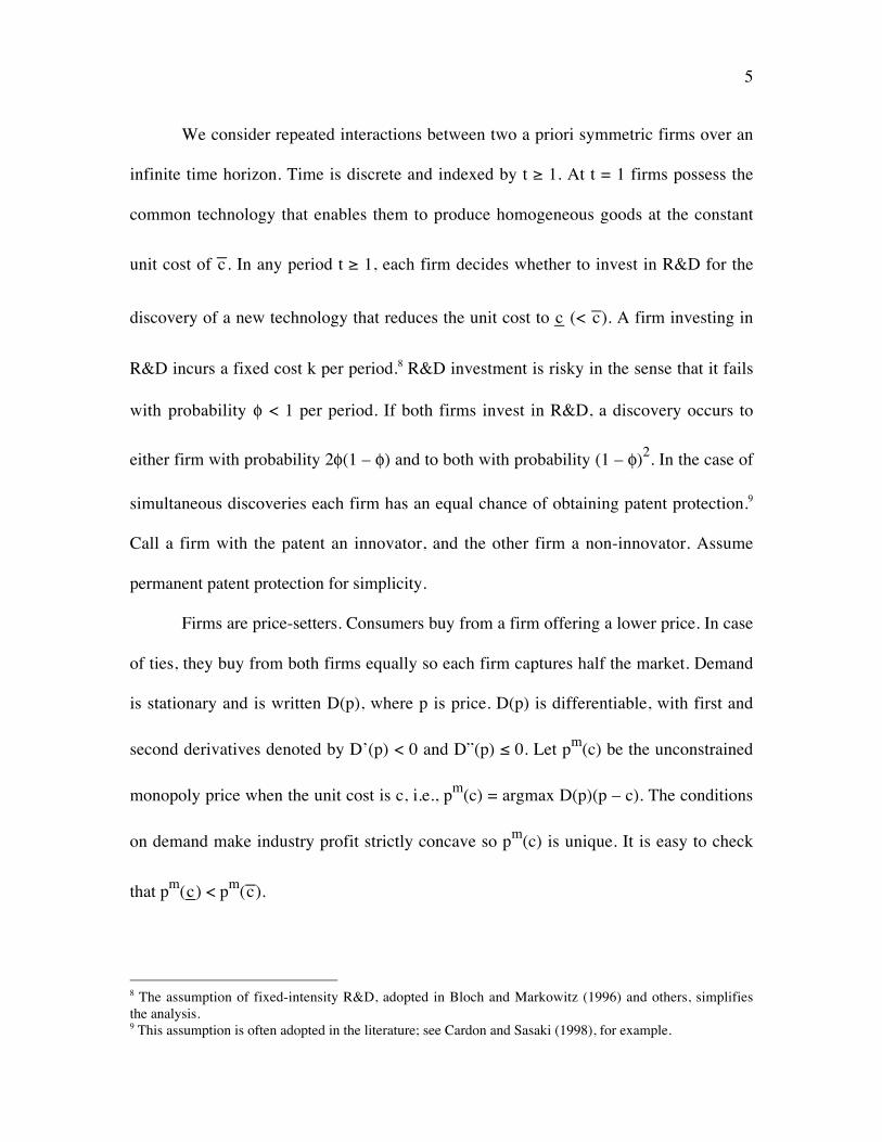
We consider repeated interactions between two a priori symmetric firms over an

infinite time horizon. Time is discrete and indexed by t ≥ 1. At t = 1 firms possess the

common technology that enables them to produce homogeneous goods at the constant

unit cost of c–. In any period t ≥ 1, each firm decides whether to invest in R&D for the

discovery of a new technology that reduces the unit cost to c– (< c–). A firm investing in

R&D incurs a fixed cost k per period.8 R&D investment is risky in the sense that it fails

with probability φ < 1 per period. If both firms invest in R&D, a discovery occurs to

either firm with probability 2φ(1 – φ) and to both with probability (1 – φ)2. In the case of

simultaneous discoveries each firm has an equal chance of obtaining patent protection.9

Call a firm with the patent an innovator, and the other firm a non-innovator. Assume

permanent patent protection for simplicity.

Firms are price-setters. Consumers buy from a firm offering a lower price. In case

of ties, they buy from both firms equally so each firm captures half the market. Demand

is stationary and is written D(p), where p is price. D(p) is differentiable, with first and

second derivatives denoted by D’(p) < 0 and D”(p) ≤ 0. Let pm(c) be the unconstrained

monopoly price when the unit cost is c, i.e., pm(c) = argmax D(p)(p – c). The conditions

on demand make industry profit strictly concave so pm(c) is unique. It is easy to check

that pm(c–) < pm(c–).

8 The assumption of fixed-intensity R&D, adopted in Bloch and Markowitz (1996) and others, simplifiesthe analysis.9 This assumption is often adopted in the literature; see Cardon and Sasaki (1998), for example.

6

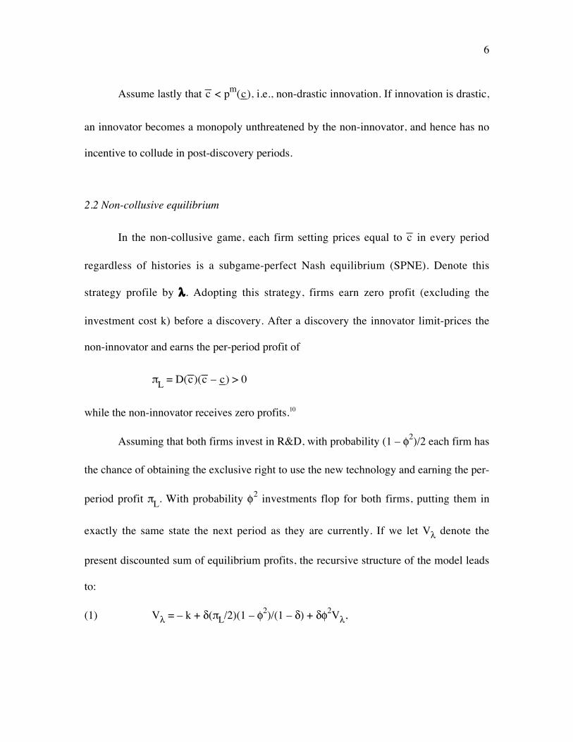
Assume lastly that c– < pm(c–), i.e., non-drastic innovation. If innovation is drastic,

an innovator becomes a monopoly unthreatened by the non-innovator, and hence has no

incentive to collude in post-discovery periods.

2.2 Non-collusive equilibrium

In the non-collusive game, each firm setting prices equal to c– in every period

regardless of histories is a subgame-perfect Nash equilibrium (SPNE). Denote this

strategy profile by λ. Adopting this strategy, firms earn zero profit (excluding the

investment cost k) before a discovery. After a discovery the innovator limit-prices the

non-innovator and earns the per-period profit of

πL = D(c–)(c– – c–) > 0

while the non-innovator receives zero profits.10

Assuming that both firms invest in R&D, with probability (1 – φ2)/2 each firm has

the chance of obtaining the exclusive right to use the new technology and earning the per-

period profit πL. With probability φ2 investments flop for both firms, putting them in

exactly the same state the next period as they are currently. If we let Vλ denote the

present discounted sum of equilibrium profits, the recursive structure of the model leads

to:

(1) Vλ = – k + δ(πL/2)(1 – φ2)/(1 – δ) + δφ2Vλ,

7

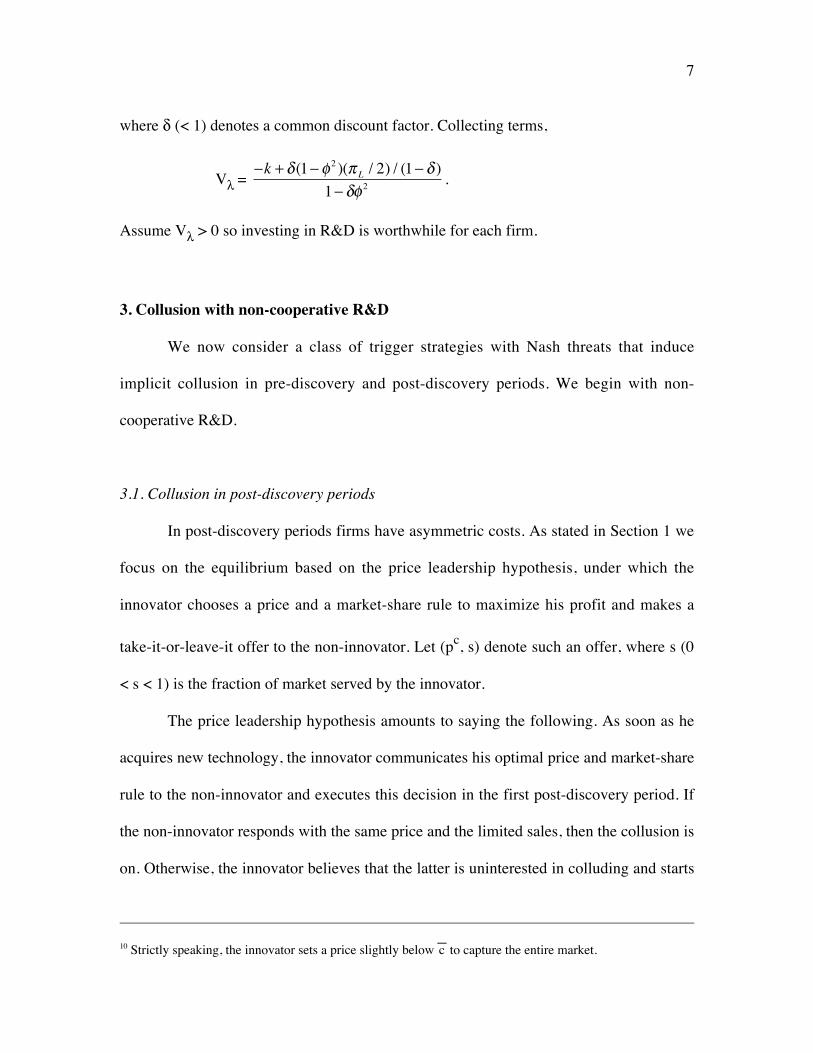
where δ (< 1) denotes a common discount factor. Collecting terms,

Vλ = −k + δ (1−φ 2 )(π L / 2) / (1− δ )

1− δφ 2.

Assume Vλ > 0 so investing in R&D is worthwhile for each firm.

3. Collusion with non-cooperative R&D

We now consider a class of trigger strategies with Nash threats that induce

implicit collusion in pre-discovery and post-discovery periods. We begin with non-

cooperative R&D.

3.1. Collusion in post-discovery periods

In post-discovery periods firms have asymmetric costs. As stated in Section 1 we

focus on the equilibrium based on the price leadership hypothesis, under which the

innovator chooses a price and a market-share rule to maximize his profit and makes a

take-it-or-leave-it offer to the non-innovator. Let (pc, s) denote such an offer, where s (0

< s < 1) is the fraction of market served by the innovator.

The price leadership hypothesis amounts to saying the following. As soon as he

acquires new technology, the innovator communicates his optimal price and market-share

rule to the non-innovator and executes this decision in the first post-discovery period. If

the non-innovator responds with the same price and the limited sales, then the collusion is

on. Otherwise, the innovator believes that the latter is uninterested in colluding and starts

10 Strictly speaking, the innovator sets a price slightly below c– to capture the entire market.

8

competing. Formally, we consider the following strategy profile. Given that there is a

discovery in period τ ≥ 1, in period τ + 1 firms set a price equal to pc and split the market

according to the market-sharing rule s. In t ≥ τ + 2, they choose (pc, s) if no other

outcomes than (pc, s) have been observed since τ + 1; otherwise they adopt the non-

collusive strategy λ forever. Denote this strategy profile by a (a mnemonic for “after” a

discovery).

We look for the condition that makes a subgame-perfect in post-discovery games.

If firms adopt a, every (post-discovery) subgame belongs to one of the two classes; one in

which all past outcomes have been (pc, s), and one in which another outcome has been

observed at least in one post-discovery period. In the latter, λ is subgame-perfect, so we

need only to show that a is subgame-perfect in the first class of subgames.

Along this collusive equilibrium path, the innovator earns the per-period profit of

πi = sD(pc)(pc – c–)

while the non-innovator earns

πn = (1 - s)D(pc)(pc – c–).

Since pc maximizes πi, put pc = pm(c–). Then, we can write the above profits as

πi = sm–, and πn = (1 – s)D[pm(c–)][pm(c–) - c–],

where m– denotes the monopoly profit:

m– ≡ D[pm(c–)][pm(c–) - c–].

9

Let vi and vn denote the sums of equilibrium profits for the innovator and the non-

innovator, respectively. The recursive structure implies

vi = πi + δvi, and vn = πn + δvn,

and hence:

vi = πi/(1 - δ) and vn = πn/(1 - δ).

Now consider a one-period deviation. A non-innovator earns D[pm(c–)][pm(c–) - c–]

one period but loses all future profits as it gets limit-priced. He thus has no incentive to

deviate if vn ≥ D[pm(c–)][pm(c–) - c–], which simplifies to

(2) δ ≥ s.

On the other hand, a devious innovator can earn m– one period and πLin all subsequent

periods. Therefore, the innovator has no incentive to deviate if

vi ≥ m– + δπL/(1 - δ),

or

δ ≥ (1 – s)m–/(m– – πL)

Thus, a is subgame-perfect in post-discovery games if

(3) δ ≥ max {(1 – s)m–/(m– – πL), s}.

Now, the innovator chooses s to maximize sm– subject to the non-innovator’s

incentive compatibility condition (2). This puts s = δ. Substituting s = δ in (3) and

rearranging yields

10

(4) δ ≥ m–/(2m– – πL) ≡ δA(c–) > 1/2.

The strategy profile a is a SPNE if and only if (4) is satisfied. Observe that δA(c–) > 1/2,

implying that a cost symmetry makes collusion more difficult to maintain.

Define cd by c– = pm(cd). Then c– > cd implies innovation is non-drastic. This next

proposition summarizes what we have found so far.

Proposition 1: Assume cd < c– < c–.

(i) The strategy profile a is a SPNE if and only δ ≥ m–/(2m– – πL) ≡ δA(c–) > 1/2.

(ii) The collusive equilibrium price and market-sharing rule are

pc = pm(c–) and s = δ > 1/2.

Since s > 1/2, the innovator has a greater market share than the non-innovator, a result

that is consistent with the findings of Bae (1987) and Harrington (1991).

The per-period equilibrium profits are

πi = δm– and πn = (1 - δ)D[pm(c–)][pm(c–) - c–].

Observe that the equilibrium profits to each firm are sensitive to the prevailing discount

factor, whereas in Bae (1987) and Harrington (1991) they are independent of it as long as

the discount factor exceeds the threshold level.

11

The locus AA in Figure 1 plots δA(c–) against c–.11 The depiction reflects the fact

that:

∂δA(c–)/∂c– = D(c–)D[pm(c–)][c– - pm(c–)]/(2m– - πL)2 < 0

for pm(c–) > c– (i.e., non-drastic innovation). It is easy to check that δA(c–) increases

towards unity as c– falls towards cd, while in the other direction it approaches 1/2 as c–

approaches c–.

Proposition 1 says that if δ < δA(c–) firms cannot collude at the monopoly price

pm(c–), but it leaves open the question whether they can collude at another price.

However, such partial collusion is impossible here. Intuitively, because the market-

sharing rule is sensitive to the discount factor in the present model, the innovator cannot

commit credibly to his offer when the discount factor falls below the critical level δA(c–).

(The proof in Appendix A.)

Lemma 1. If δ < δA(c–), partial collusion is impossible in post-discovery subgames.

3.2. Collusion in pre-discovery periods

11 We limit analysis to δ ≥ 1/2.

12

We now turn to the stability of collusion in pre-discovery periods. Consider the

following symmetric strategy: In t = 1, set a price equal to pm(c–), the monopoly price

under the old technology. In any pre-discovery period t ≥ 2, there are four possible states

of nature.

(i) No other prices than pm(c–) have been observed and there was a discovery in t – 1.

(ii) No other prices than pm(c–) have been observed and there has been no discovery to

date.

(iii) Prices other than pm(c–) have been observed at least once in the past and there was a

discovery in t – 1.

(iv) Prices other than pm(c–) have been observed at least once in the past and there has

been no discovery to date.

In state (i), adopt a. In state (ii) set the price equal to pm(c–). In states (iii) and (iv) adopt

λ. Call this strategy profile b (a mnemonic for “before” a discovery).

Since b is subgame-perfect in states (i), (iii) and (iv), we need only to check state

(ii). In state (ii) the equilibrium payoff, denoted by Vc, satisfies this recursive equation

(5) Vc = m–/2 − k + δ(1 − φ2)(vi + vn)/2 + δφ2Vc,

where m– denotes the monopoly profit under the old technology; i.e.,

m– = D[pm(c–)][pm(c–) – c–).

Collecting terms in (5) yields

13

Vc = m/2 − k + δ(1−φ 2 )(vi + vn )/21 - δφ 2 .

Consider now a one-period deviation. A deviating firm earns (m– – k) but finds

itself in state (iii) or state (iv) the next period, with a switch to λ, thereby receiving the

following expected profits:

m– − k + δ(1 − φ2)(πL/2)/(1 − δ) + δφ2Vλ = m– + Vλ

where (1) is used to get to the right-hand side. A deviation is unprofitable if this profit is

less than Vc, i.e.,

(6) Vc – Vλ ≥ m–,

where

(7) Vc – Vλ = δ(1 – φ2)[vi + vn - πL/(1 – δ)]/2 + m–/2

1 – δφ2 .

The difference in profits, Vc – Vλ, between the collusive and the competitive paths

increases without bounds as δ goes to unity, so (6) holds with strict inequality for a high

enough δ < 1. On the other hand, when δ is sufficiencly close to 1/2, (6) fails, as shown in

Appendix B. Therefore, there exists a unique δ ∈(1/2, 1) at (6) holds with strict equality,

which we denote by δB(c–).

The locus BB (comprising the thick and dotted segments) in Figure 1 plots δB(c–)

against c–, assuming that firms maintain the collusive equilibrium in post discovery

14

periods and that φ2 ≥ 1/2. The depiction is based on the following lemma (see Appendix

C for a proof):

Lemma 2: Given that cd < c– < c–

(i) ∂δB(c–)/∂c– < 0

(ii) 1/2 < δB(c–) < 1/(2φ2).

(iii) If φ2 ≥ 1/2, there is a point (c–, δ(c–)) at which the loci AA and BB intersect.12

Thus, the locus BB curves upward as c– falls but stays strictly between 1/2 and 1/(2φ2). If

φ2 < 1/2, however, the upper bound exceeds unity, implying that the locus BB may stay

above the locus AA for all c– > cd.

Finally, the analysis of this subsection is predicated on there being collusion in

post-discovery periods, i.e., δ ≥ δA(c–). Thus, we have

Proposition 2: If δ ≥ max {δA(c–), δB(c–)} > 1/2, the strategy profile b is subgame-perfect

and entails collusion in pre-discovery and post-discovery periods.

12 This establishes the existence. There may be more than one such point. However, the results we showbelow do not depend on the uniqueness.

15

The prospect that collusion is less stable in post-discovery periods due to a cost

asymmetry makes collusion more difficult to maintain in pre-discovery periods, during

which costs are still symmetric. In terms of Figure 1, collusion is sustainable before and

after a discovery if and only the (δ, c–) pair is in Region 1 defined by the set {(δ, c–)|

δ ≥ max {δA(c–), δB(c–)}}. Outside Region 1, the strategy profile b cannot support

collusion.13 In Region 2 defined by the set {(δ, c–)| δA(c–) ≤ δ < δB(c–)}, for example, firms

can maintain full collusion after a discovery but not before because the monopoly price

pm(c–) cannot satisfy the no-deviation condition (6). The question is: can firms collude

partially, that is, at a price different from the monopoly price pm(c–) until there is a

discovery? As in the post-discovery game, the next lemma shows they cannot (the proof

in Appendix D).

Lemma 3. If δA(c–) ≤ δ < δB(c–) there is no partial collusion in pre-discovery periods.

Thus, in Region 2, although they cannot collude in pre-discovery periods, firms can fully

collude in post-discovery periods by playing a competitive one-shot game until there is a

discovery and then switch to playing a. This is a SPNE, yielding zero profits (minus

investment cost k) until a discovery and m–/2 per period afterwards.

13 It is always possible to maintain collusion at prices below the monopoly price outside Region 1. To keepthe analysis compact such partial collusion is ruled out, so firms choose either full collusion (at themonopoly prices) or competition.

16

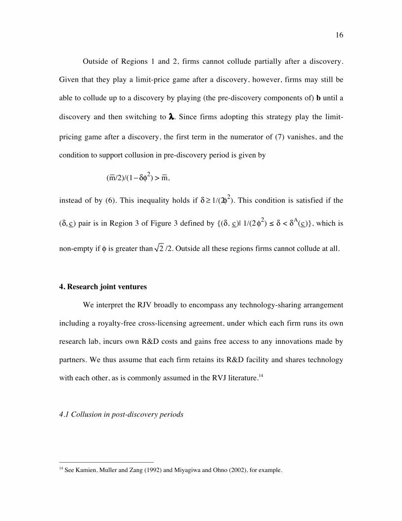
Outside of Regions 1 and 2, firms cannot collude partially after a discovery.

Given that they play a limit-price game after a discovery, however, firms may still be

able to collude up to a discovery by playing (the pre-discovery components of) b until a

discovery and then switching to λ. Since firms adopting this strategy play the limit-

pricing game after a discovery, the first term in the numerator of (7) vanishes, and the

condition to support collusion in pre-discovery period is given by

(m–/2)/(1 − δφ2) > m–,

instead of by (6). This inequality holds if δ ≥ 1/(2 φ2). This condition is satisfied if the

(δ, c–) pair is in Region 3 of Figure 3 defined by {(δ, c–)| 1/(2 φ2) ≤ δ < δA(c–)}, which is

non-empty if φ is greater than 2 /2. Outside all these regions firms cannot collude at all.

4. Research joint ventures

We interpret the RJV broadly to encompass any technology-sharing arrangement

including a royalty-free cross-licensing agreement, under which each firm runs its own

research lab, incurs own R&D costs and gains free access to any innovations made by

partners. We thus assume that each firm retains its R&D facility and shares technology

with each other, as is commonly assumed in the RVJ literature.14

4.1 Collusion in post-discovery periods

14 See Kamien, Muller and Zang (1992) and Miyagiwa and Ohno (2002), for example.

17

Suppose there is a discovery in period τ ≥ 1 and the firms adopt the following

post-discovery strategy, denoted by α. In τ + 1, set a price equal to the monopoly price

pm(c–) under the new technology. In all t + τ, (t ≥ 2), choose pm(c–) if no other prices than

pm(c–) have been observed since τ + 1; otherwise set a price to c–. Thus, α is a standard

collusive strategy profile for symmetric price-setting duopoly and is a SPNE for δ ≥ 1/2.

Compared with Proposition 1, this result shows that formation of an RJV facilitates

collusion in post-discovery periods by preventing a cost symmetry from arising, which

tends to stabilize collusion before a discovery. The question is how low the threshold

discount factor falls. We turn to this question next.

4.2 Collusion in pre-discovery periods

Consider the following collusive strategy denote by β:

In t = 1, set a price equal to the monopoly price pm(c–). In any pre-discovery period t ≥ 2,

there are four possible states of nature.

(i) No other prices than pm(c–) have been observed, and there was a discovery in t – 1.

(ii) No other prices than pm(c–) have been observed and there has been no discovery to

date.

18

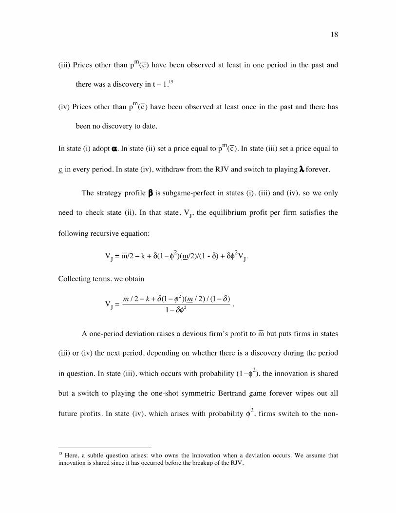
(iii) Prices other than pm(c–) have been observed at least in one period in the past and

there was a discovery in t – 1.15

(iv) Prices other than pm(c–) have been observed at least once in the past and there has

been no discovery to date.

In state (i) adopt α. In state (ii) set a price equal to pm(c–). In state (iii) set a price equal to

c– in every period. In state (iv), withdraw from the RJV and switch to playing λ forever.

The strategy profile β is subgame-perfect in states (i), (iii) and (iv), so we only

need to check state (ii). In that state, VJ, the equilibrium profit per firm satisfies the

following recursive equation:

VJ = m–/2 – k + δ(1 − φ2)(m–/2)/(1 - δ) + δφ2VJ.

Collecting terms, we obtain

VJ = m / 2 − k + δ (1−φ2 )(m / 2) / (1− δ )

1− δφ 2.

A one-period deviation raises a devious firm’s profit to m– but puts firms in states

(iii) or (iv) the next period, depending on whether there is a discovery during the period

in question. In state (iii), which occurs with probability (1 − φ2), the innovation is shared

but a switch to playing the one-shot symmetric Bertrand game forever wipes out all

future profits. In state (iv), which arises with probability φ2, firms switch to the non-

15 Here, a subtle question arises: who owns the innovation when a deviation occurs. We assume thatinnovation is shared since it has occurred before the breakup of the RJV.

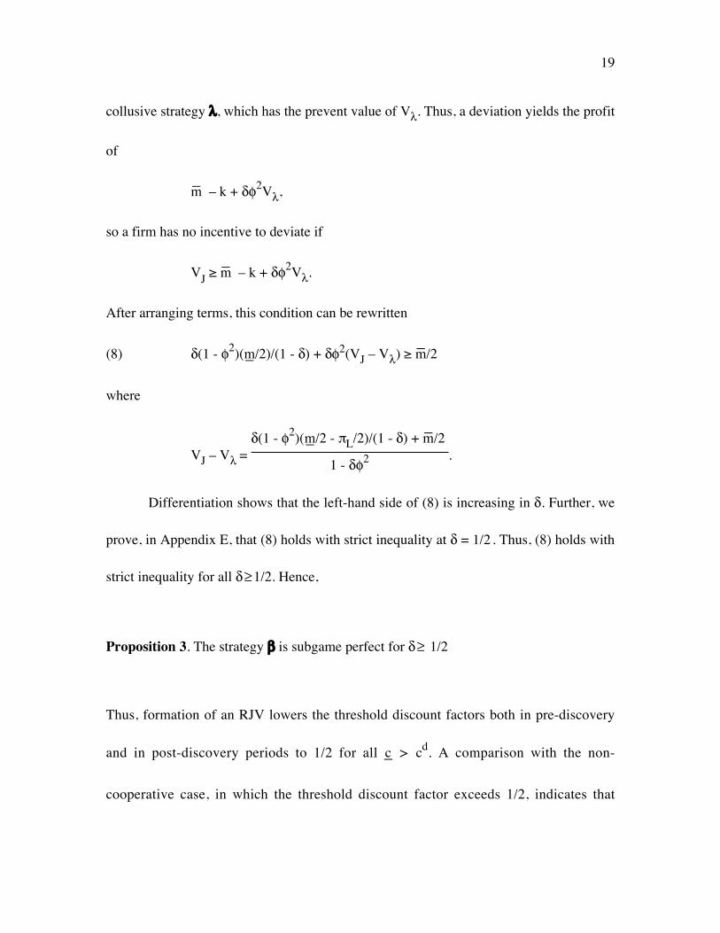
19

collusive strategy λ, which has the prevent value of Vλ. Thus, a deviation yields the profit

of

m– – k + δφ2Vλ,

so a firm has no incentive to deviate if

VJ ≥ m– – k + δφ2Vλ.

After arranging terms, this condition can be rewritten

(8) δ(1 - φ2)(m–/2)/(1 - δ) + δφ2(VJ – Vλ) ≥ m–/2

where

VJ – Vλ = δ(1 - φ2)(m–/2 - πL/2)/(1 - δ) + m–/2 

1 - δφ2 .

Differentiation shows that the left-hand side of (8) is increasing in δ. Further, we

prove, in Appendix E, that (8) holds with strict inequality at δ = 1/2 . Thus, (8) holds with

strict inequality for all δ ≥ 1/2. Hence,

Proposition 3. The strategy β is subgame perfect for δ ≥ 1/2

Thus, formation of an RJV lowers the threshold discount factors both in pre-discovery

and in post-discovery periods to 1/2 for all c– > cd. A comparison with the non-

cooperative case, in which the threshold discount factor exceeds 1/2, indicates that

20

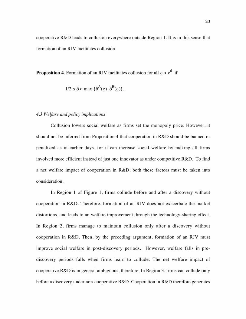
cooperative R&D leads to collusion everywhere outside Region 1. It is in this sense that

formation of an RJV facilitates collusion.

Proposition 4. Formation of an RJV facilitates collusion for all c– > cd if

1/2 ≤ δ < max {δA(c–), δB(c–)}.

4.3 Welfare and policy implications

Collusion lowers social welfare as firms set the monopoly price. However, it

should not be inferred from Proposition 4 that cooperation in R&D should be banned or

penalized as in earlier days, for it can increase social welfare by making all firms

involved more efficient instead of just one innovator as under competitive R&D. To find

a net welfare impact of cooperation in R&D, both these factors must be taken into

consideration.

In Region 1 of Figure 1, firms collude before and after a discovery without

cooperation in R&D. Therefore, formation of an RJV does not exacerbate the market

distortions, and leads to an welfare improvement through the technology-sharing effect.

In Region 2, firms manage to maintain collusion only after a discovery without

cooperation in R&D. Then, by the preceding argument, formation of an RJV must

improve social welfare in post-discovery periods. However, welfare falls in pre-

discovery periods falls when firms learn to collude. The net welfare impact of

cooperative R&D is in general ambiguous, therefore. In Region 3, firms can collude only

before a discovery under non-cooperative R&D. Cooperation in R&D therefore generates

21

no welfare change in pre-discovery periods, but a welfare loss in post-discovery periods

as the market gets monopolized. Thus cooperation in R&D lowers social welfare.

Similarly, welfare falls unambiguously outside the three regions.

To sum, formation of an RJV can increase social welfare only if the collusive

equilibrium is maintained in post-discovery periods in the absence of cooperation in

R&D. Thus we have a counterintuitive result: a cost-cutting technology drives welfare

improvements under cooperative R&D, but welfare is likely to fall when there is too

sharp a cost reduction under new technology. This has the obvious policy implication for

antitrust authorities: firms should be more closely monitored for anticompetitive behavior

when they form an RJV aiming for a major technological breakthrough.

5. Extensions

In section we relax some of the assumptions of the model. They are (i) non-drastic

innovation, (ii) permanent patent protection, and (iii) Nash threats (punishment by

reversions to repeated play of a one-shot game).

First, suppose innovation is drastic as in Martin (1995). With drastic innovation

an innovator becomes a monopoly so there is no collusion in post-discovery periods.

Thus, the analysis is similar to the one associated with Region 3; namely, formation of an

RJV facilitates collusion in post-discovery periods and lowers social welfare, which is

exactly what Martin (1995) has argued.

Second, suppose that patent life is finite. If patent life is, say, T periods, the value

of new technology to the innovator falls from πL/(1 - δ) under permanent patent

22

protection to πL(1 - δT)/(1 − δ).16 In the collusive equilibrium finite patent life thus

decreases the value of a deviation, thereby making collusion easier to maintain both

before and after a discovery.

Third, it is well known in the implicit collusion literature that collusion can be

sustained for a lower range of discount factors if firms can commit to a severer

punishment scheme than Nash reversions. In a recent paper Thal (2006) considers such a

scheme for Bertrand duopoly with asymmetric costs and finds that a credible punishment

strategy with an Abreu (1986, 1988) stick-and-carrot structure reduces the payoff to the

firm with lowest cost to zero. Although not concerned with the uniqueness of equilibrium

selection, when applied to our model, her analysis implies that there is an optimal

punishment scheme that can reduce the threshold discount factor after a discovery to 1/2

without formation of an RJV. However, it is not clear whether the threshold discount

factor also falls to 1/2 in pre-discovery periods. We show in Appendix F, however, that

that is the case under the assumption of linear demand. In that case, firms can collude

before and after a discovery at any discount factor greater or equal to 1/2 without forming

an RJV, meaning cooperation in R&D always improve social welfare.

6. Summary

We examine whether cooperation in R&D leads to product market collusion. Our

basic model has firms managing implicitly to maintain the collusive equilibrium while

engaged in a stochastic R&D race. Under competitive R&D innovation gives rise to an

16 In period T + 1 the technology becomes public and competition wipes out profits for the innovator.

23

inter-firm cost asymmetry and can destabilizes collusion when the discount factor is low

or the cost reduction under new technology is large. The prospect that collusion ends with

innovation further destabilizes collusion in pre-discovery periods. Cooperation in R&D

preserves a cost symmetry through innovation sharing, and leads to more collusion in

product markets. However, cooperation in R&D does not necessarily decrease social

welfare, as sharing of new technology improves efficiency in production. Although new

technology is the driving force for a welfare improvement, cooperation in R&D is more

likely to decrease welfare if the cost falls too much under new technology.

24

Appendices

Appendix A: Proof of Lemma 1. Let δ < δA(c–) be given. Suppose there is a pair (p*, s*),

where p* ≠ pm(c–), such that p* maximizes the innovator’s profit s*m–* = s*D(p*)(p* - c–)

and satisfies the no-deviation constraints for both the innovator and the non-innovator.

Case 1. p* < pm(c–)

Partial collusion is stable if

δ ≥ max {(1 – s*)m–*)/(m–* – πL), s*}

If δ ≥ (1 – s*)m–*)/(m–* – πL) > s*, s* can be increased up to δ, increasing the profit to the

innovator, without violating the no-deviation constraint. So, at the optimum the innovator

sets s* = δ. Therefore, we have

δ ≥ (1 – δ)m–*/(m–* – πL)

or

δ ≥ m–*/(2m–* – πL).

But the right-hand side is decreasing in m* for 0 ≤ m–*≤ m–, and hence

δ ≥ m–*/(2m–* – πL) > m–/(2m– – πL) = δA(c–),

which contradicts the assumption δ < δA(c–).

Case: pm(c–) < p* < pm(c–)

There is no deviation if

25

δ ≥ max {(m– - s*m–*)/(m– – πL), s*}.

Again, s* can be increased up to δ without violating this constraint so δ = s*. We can

write the above as

δ ≥ (m– - δm–*)/(m– – πL).

that is,

δ ≥ m–/(m– – πL + m–*).

But since m–* < m–

δ ≥ m–/(m– – πL + m–*) > m–/(2m– – πL) = δA(c–),

a contradiction.

Case 3: p* ≥ pm(c–).

The innovator does not deviate if

δ ≥ [m– - (1 – s*)m–*]/m–,

and the non-innovator does not if

δ ≥ (m– – s*m–*)/(m– – πL).

Partial collusion is sustained if both conditions hold. The first must hold with equality,

for otherwise the innovator can increase profit by raising s*. Therefore, s* satisfies

(1 - δ)m– = (1 – s*)m–*.

Using this the second condition can be writte

δ(m– – πL) ≥ (m– – s*m–*) = m– + (1 - δ)m– – m–*

26

Collecting terms,

δ ≥ [m– + m– – m–*]/[(m– – πL + m–] > m–/(2m– – πL) = δA(c–),

a contradiction. ❏

Appendix B: We show that (6) fails at δ = 1/2. Assume the contrary, and evaluate (6) at δ

= 1/2 to obtain this equivalent condition:

(A1) m– + D[pm(c–)][pm(c–) – c–] – πL – 2m– ≥ 0.

However, we can express the left-hand side of (A1) as

D[pm(c–)][2pm(c–) – c– – c–] – D(c–)(c– – c–) – 2D[pm(c–)][pm(c–) – c–)

< 2D(c–)[pm(c–) – c–] – 2D[pm(c–)][pm(c–) – c–)

< 0,

where the first inequality is obtained from substitution of D(c–) for D[pm(c–)] while the

second follows the fact that pm(c–) is the profit-maximizing price at cost c–. This

contradiction is what we wanted. ❏

Appendix C: We prove Lemma 2. Proof of Result (i) dδB(c–)/dc– < 0. Write δB(c–) = δBto

save space. δB is implicitly defined by (6) or satisfies this implicit function

g(δB, c–) ≡ VJ – Vλ – m– = 0.

27

where VJ – Vλ is given by (7). Write g(δB, c–) = g. Straightforward differentiation of (7)

shows that ∂g/∂δB > 0. On the other hand,

sgn {∂g/∂c–} = sgn {∂(VJ – Vλ)/∂c–} = sgn {∂(πi + πn – πL)/∂c–}

The last derivative is

– δBD[pm(c–)] + D(c–) > 0

since pm(c–) > c–. Therefore, by the implicit-function theorem we conclude that

dδB(c–)/dc– = – (∂g/∂c–)/(∂g/∂δB) < 0.

Proof of Result (ii): As c– approaches cd, Vc – Vλ approaches (m–/2)(1 − δφ2). Therefore, if

δ > 1/(2φ2), (6) holds with strict inequality at the limit c– = cd, that is,

(m–/2)/(1 − δφ2) > m–.

This implies that δB(c–) is bounded from above by 1/(2φ2).

Proof of Result (iii). Suppose that φ2 ≥ 1/2. Then 1/(2φ2) ≤ 1. Hence, 1 > δB(c–) > 1/2 by

Result (ii) of this lemma. On the other hand, δA(c–) approaches unity as c– approaches cd,

and approaches 1/2 as c– nears c–. Thus, the two loci cross each other. ❏

Appendix D. We prove Lemma 3: Let δ be given such that δA(c–) ≤ δ < δB(c–). Suppose

there is a price p* ≠ pm(c–) and the total profit m–* = D(p*)(p* - c–) < m– satisfying

28

δ(1 – φ2)[vi + vn - πL/(1 – δ)]/2 + m–*/2

1 – δφ2 ≥ m–*

Byt firms cannot collude fully so

m– > δ(1 – φ2)[vi + vn - πL/(1 – δ)]/2 + m–/2

1 – δφ2 .

Adding and simplifying

[m– - m–*]/[2(1 - δφ2)] ≥ m– - m–*

which holds only if

δ >1/ (2φ2).

By Lemma 2,

1/(2φ2) > δB(c–).

These two imply δ > δB(c–), a contradiction. ❏

Appendix E: We show that (8) holds with strict inequality at δ = 1/2. First we show:

(D1) m– – πL – m–

= D[pm(c–)][pm(c–) – c–] – D(c–)(c– – c–) – D[pm(c–)][pm(c–) – c–)

> D[pm(c–)][pm(c–) – c–] – D(c–)(c– – c–) – D(c–)[pm(c–) –c–)

= D[pm(c–)][pm(c–) – c–] – D(c–)[pm(c–) – c–) > 0.

Second, evaluate VJ – Vλ at δ = 1/2 to obtain

29

VJ – Vλ = (1 - φ2)(m–  – πL) + m–  

2 - φ2 .

Subtract m– from it.

(D2) VJ – Vλ – m– = (1 - φ2)(m– – πL – m–)/(2 - φ2) > 0

by (D1). Finally, evaluate the left-hand side of (8) at δ = 1/2 to obtain

(D3) (1 – φ2)m–/2 + φ2(VJ – Vλ)/2

> (1 – φ2)m–/2 + φ2m–/2

> m–/2,

where the first inequality uses (D2). But (D3) shows that (8) holds with strict inequality

at δ = 1/2. ❏

Appendix F: Since he receives zero profits following a deviation, the innovator has no

incentive to deviate if sm–/(1 – δ) ≥ m–, or s ≥ 1 – δ. Likewise, the non-innovator does not

deviate if s ≤ δ. Thus, 1 – δ ≤ s ≤ δ. At δ = 1/2, this means s = 1/2. Now, modify the pre-

discovery components of b as follows. In state (iv) firms set price equal to c– until a

discovery, after which they switch to the stick-and-carrot strategy described by Thal

(2006). Then, a one-period deviation before a discovery yields zero profits (excluding k)

past the period in which a deviation occurs, regardless of histories. It follows that a

30

deviant firm chooses not to invest in R&D investment. With this modification, (6)

becomes

Vc ≥ m–.

Substituting δ = 1/2 and canceling terms, we can write this condition as

m– + D[pm(c–)][pm(c–) – c–] – 2m– ≥ 0.

This condition may or may not hold in general but it does hold under the assumption of

linear demand as can easily be confirmed by directly evaluation of the profits. If it does,

then firms can maintain collusion before and after innovation at any δ ≥ 1/2 as under

cooperative R&D. ❏

31

References

Abreu, D., 1986, Extremal equilibria of oligopolistic supergames, Journal of Economic

Theory 39, 191-225.

Abreu, D., 1988, Towards a theory of discounted repeated game, Econometrica 56, 383-

396

Bae, Y., 1987, A price-setting supergame between heterogeneous firms, European

Economic Review 31, 1159-1171

Bloch, F., and Markowitz, P, 1996, Optimal disclosure delay in multistage R&D

competition, International Journal of Industrial Organization 14, 159-179

Cabral, L. M. B., 2000, R&D cooperation and product market competition, International

Journal of Industrial Organization 18, 1033-1047

Caloghirou, Y., S. Ioannides, and N.S. Vonortas, 2003, Research joint ventures, Journal

of Economic Surveys 17, 541-570

Cardon, J. H. and Sasaki, D., 1998, Preemptive search and R&D clustering, RAND

Journal of Economics 29, 324-338

Collie, D.R., 2004, Sustaining collusion with asymmetric costs, unpublished paper.

D’Aspremont, C, and Jacquemin, A., 1988, Cooperative and noncooperative R&D in

duopoly with spillovers, American Economic Review 78, 1133-1137.

Friedman, J.W., 1971, A non-cooperative equilibrium for supergames, Review of

Economic Studies 38, 1 – 12.

Harrington, Jr., J. E., 1991, The determination of price and output quotas in a

heterogeneous cartel, International Economic Review 32, 767-792

32

Kamien, M. I., E. Muller, and I. Zang, 1992, Research joint ventures, and R&D cartels,

American Economic Review 82, 1293-1306.

Lambertini, L., S. Poddar and D. Sasaki, 2002, Research joint ventures, product

differentiation, and price collusion, International Journal of Industrial

Organization 20, 829-854

Lambertini, L., S. Poddar and D. Sasaki, 2003, RJVs in product innovation and cartel

stability, Review of Economic Design 7, 465-477.

Martin, S., 1995, R&D joint ventures and tacit product market collusion, European

Journal of Political Economy 11, 733-741

Miyagiwa, K., and Y. Ohno, 2002, Uncertainty, spillovers, and cooperative R&D,

International Journal of Industrial Organization, 855-876

Rothschild, R., 1999, Cartel stability when costs are heterogeneous, International Journal

of Industrial Organization 17, 717-734

Thal, J., Optimal collusion under cost asymmetry, unpublished paper

Verboven, F., 1997, Collusive behavior with heterogeneous firms, Journal of Economic

Behavior and Organization 33, 121-136

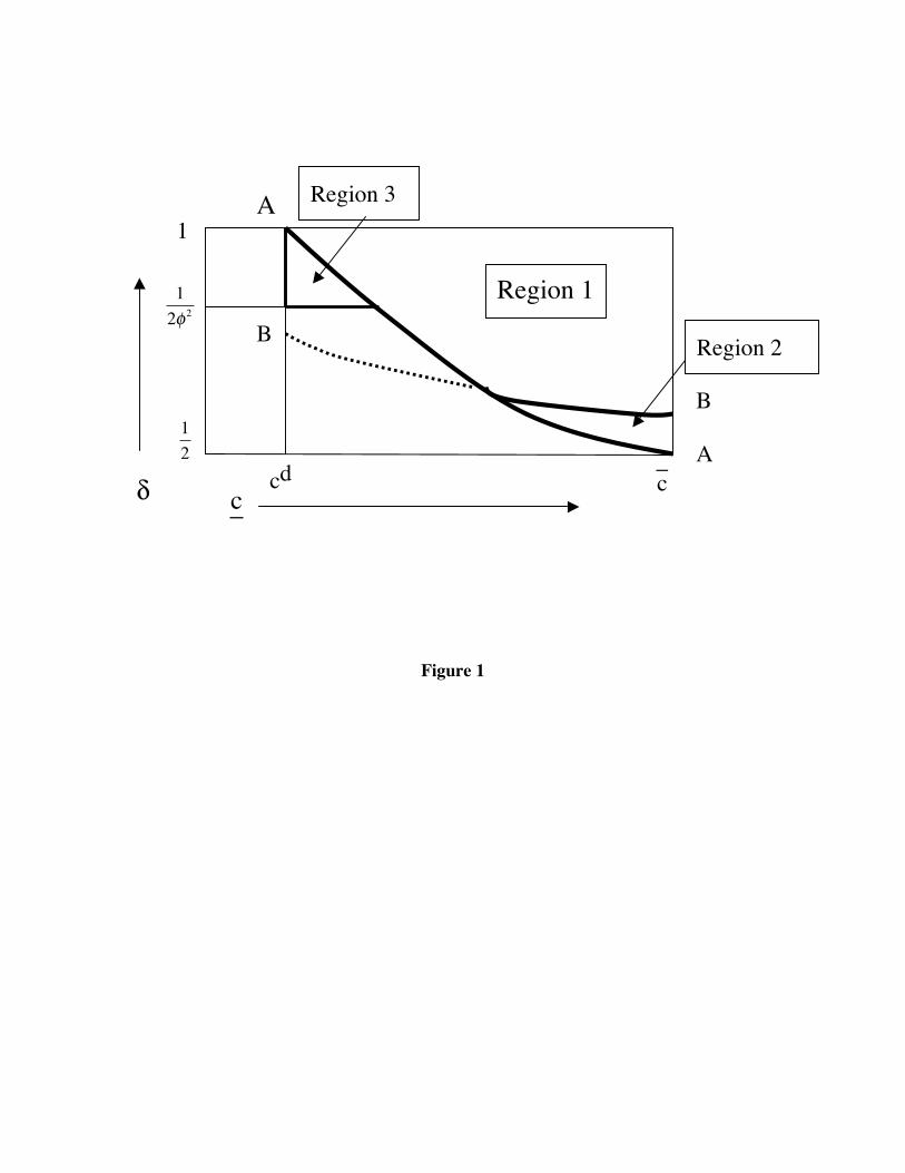
Figure 1

A

A

B

B

Region 1

Region 2

Region 3

12

cd

1

12φ 2

δ c–c–