Embed Size (px)
Citation preview
Colloquium, School of MathematcsUniversity of Minnesota, October 5, 2006
Computing the Genus of a Curve Numerically
Andrew SommeseUniversity of Notre Dame
In collaboration with
Daniel Bates, IMA
Christopher Peterson, Colorado State University
Charles Wampler, General Motors R&D Center
2
Reference on Numerical Algebraic Geometry up to 2005: A.J. Sommese and C.W. Wampler, Numerical
solution of systems of polynomials arising in engineering and science, (2005), World Scientific Press.
Website with more information and some articles: www.nd.edu/~sommese
3
Overview
What is an algebraic curve? What is the genus of a curve? An example from applications
Four-bar-planar linkage coupler curves Background on Numerical Algebraic Geometry
How to represent Positive Dimensional Solution Sets Numerical approach by using Hurwitz’s formula
4
What is an algebraic curve?
Curves are ancient, beautiful, and useful. They are pervasive in mathematics: in
number theory, algebraic, analytic, and differential geometry, complex analysis, numerical analysis, topology,...
The arise everywhere in applications.
5
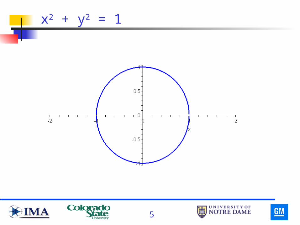
x2 + y2 = 1
6
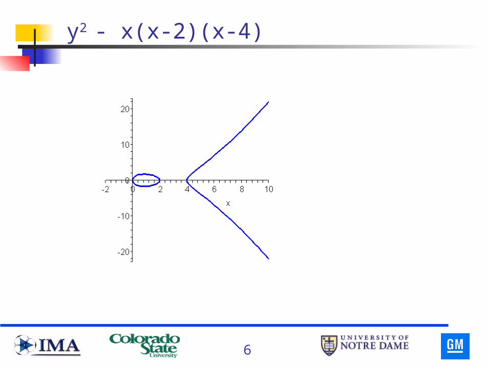
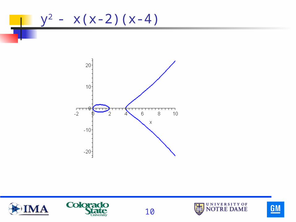
y2 - x(x-2)(x-4)
7
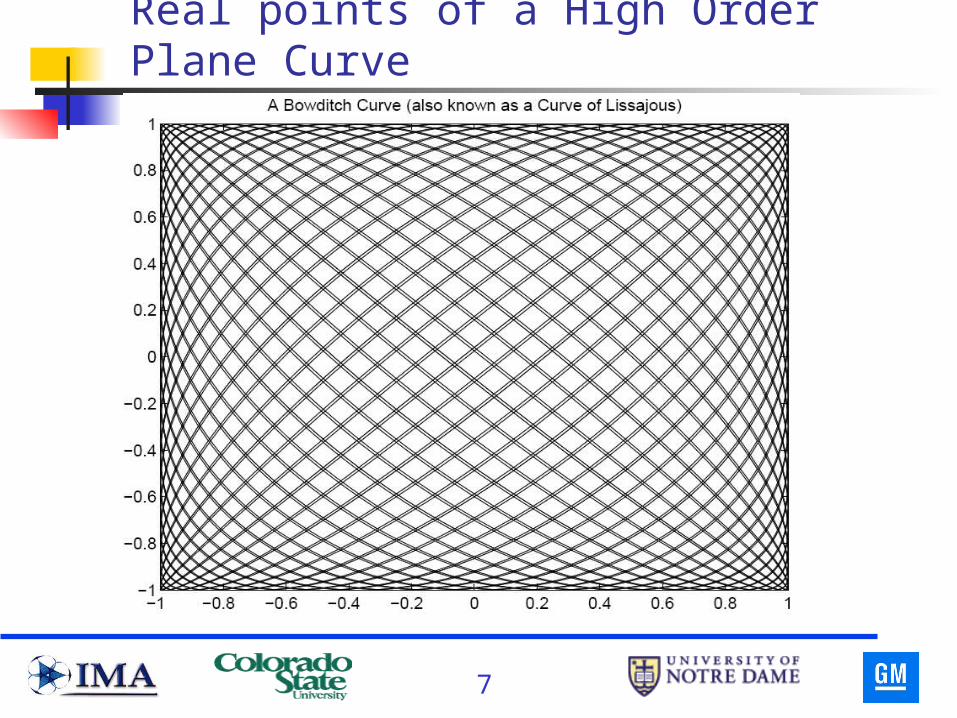
Real points of a High Order Plane Curve
8
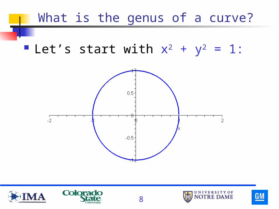
What is the genus of a curve?
Let’s start with x2 + y2 = 1:
9
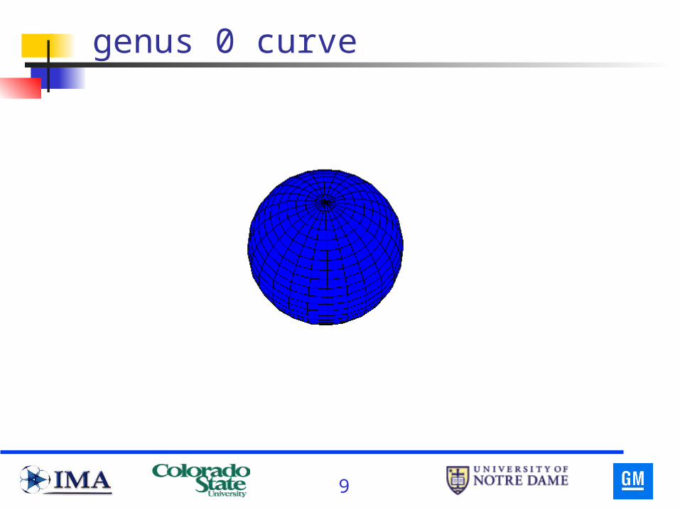
genus 0 curve
10
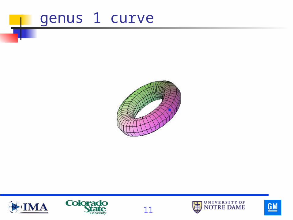
y2 - x(x-2)(x-4)
11
genus 1 curve
12
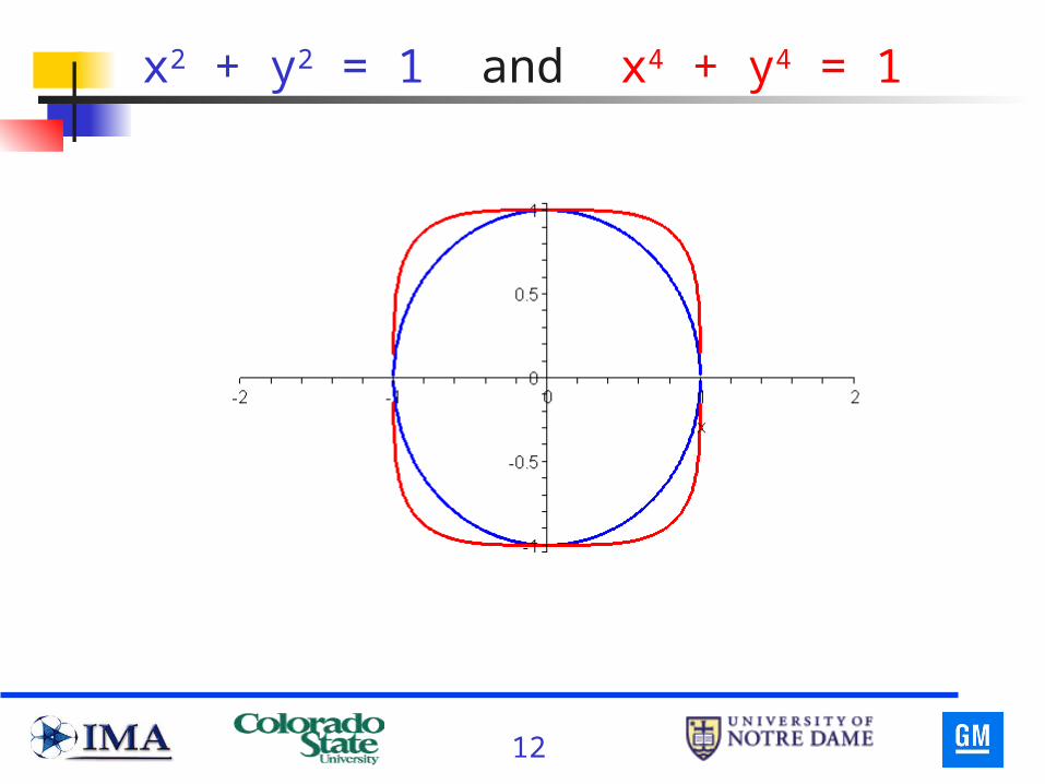
x2 + y2 = 1 and x4 + y4 = 1
13
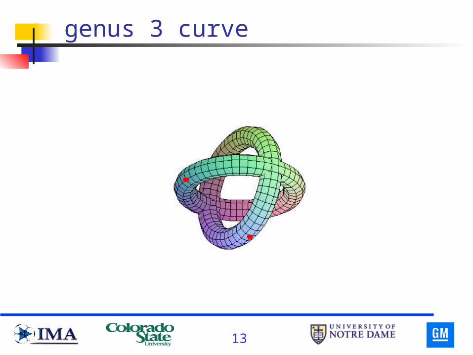
genus 3 curve

14
Interlude between slides
Including blackboard discussion of the examples; the Euler characteristic; and Hurwitz’s formula.
15
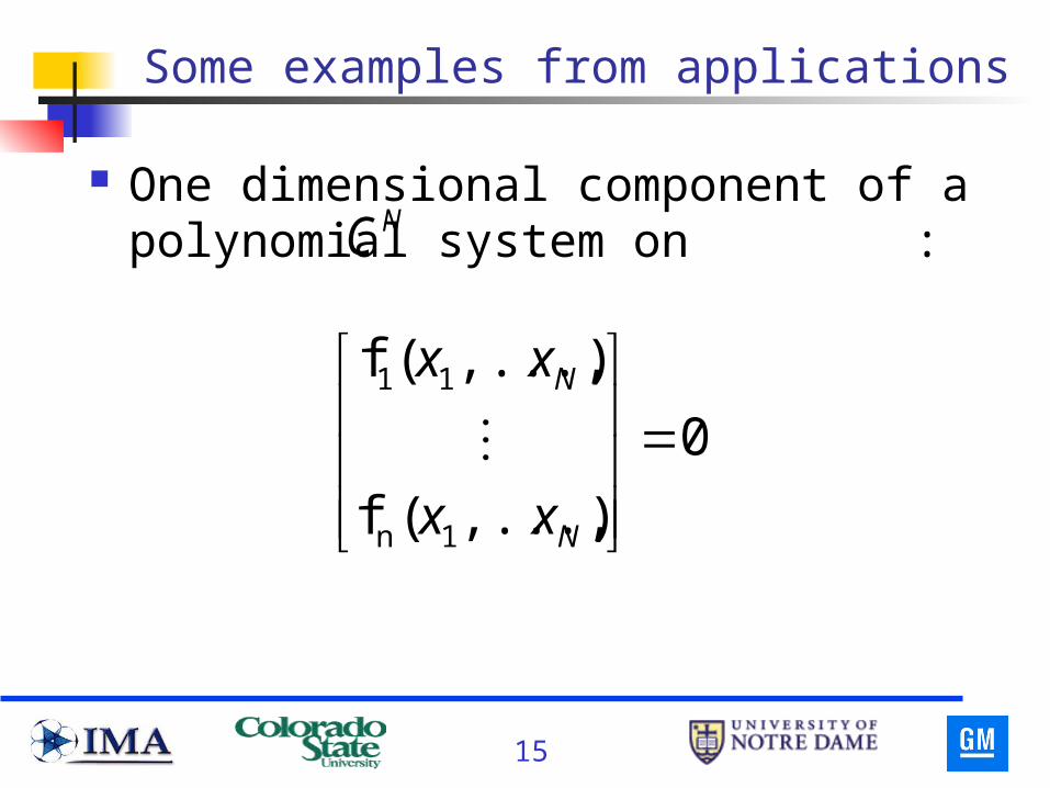
Some examples from applications
One dimensional component of a polynomial system on :
0
),...,(f
),...,(f
1n
11
N
N
xx
xx
NC
16
Planar four-bar coupler curves
A four-bar planar linkage is a planar quadrilateral with a rotational joint at each vertex.
They are useful for converting one type of motion to another.
They occur everywhere.
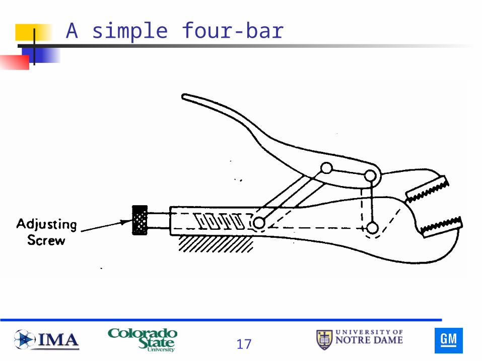
17
A simple four-bar
18
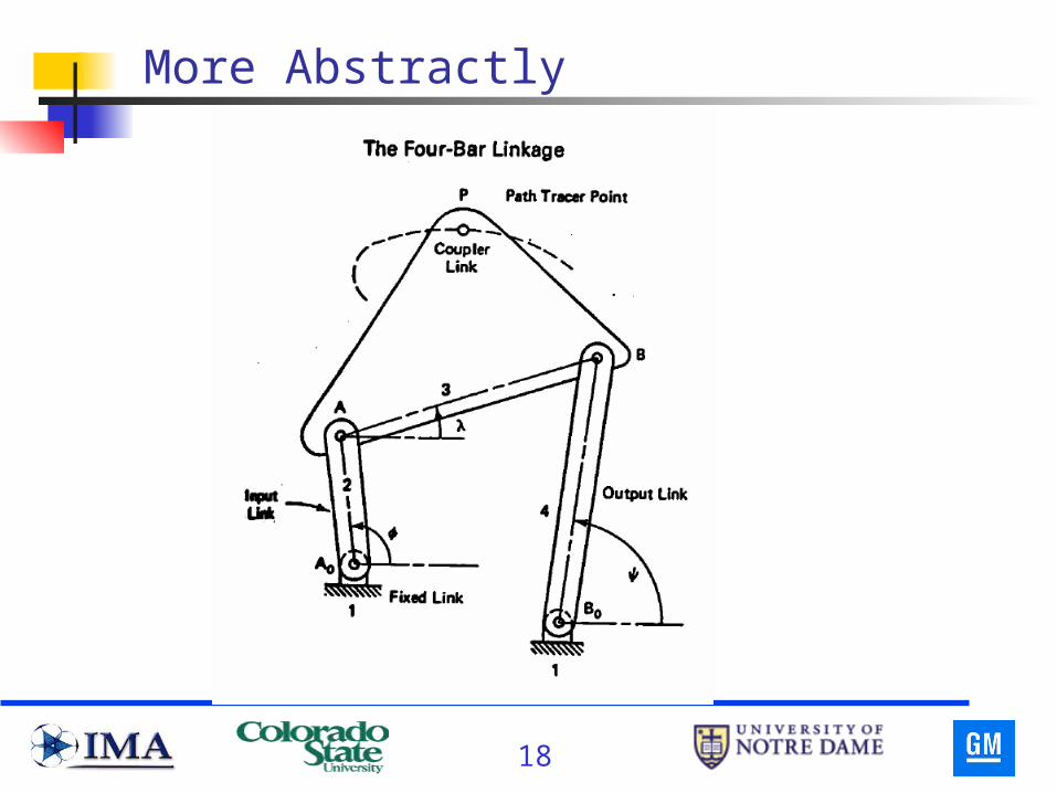
More Abstractly
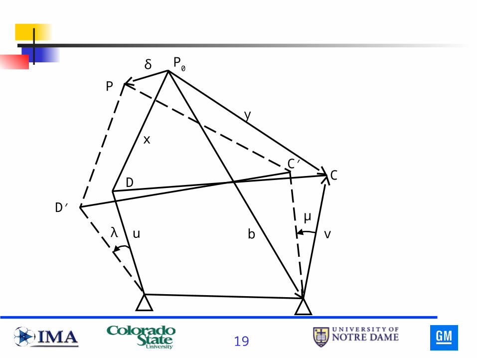
19
D′
P
δ
λµ
u b v
CD
x
y
P0
C′
20
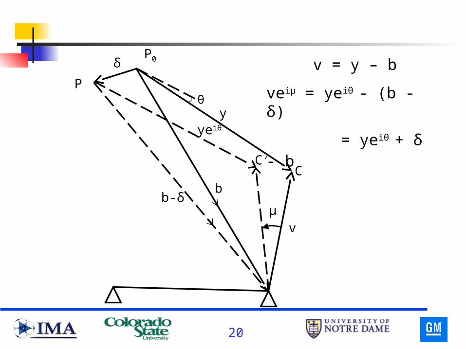
P
δ
µb-δ
v
C
y
P0
θ
yeiθ
b
v = y – b
veiμ = yeiθ - (b - δ)
= yeiθ + δ - b
C′
21
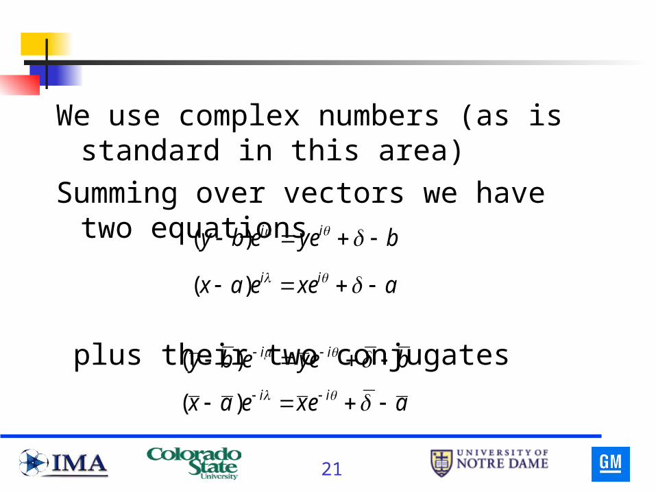
We use complex numbers (as is standard in this area)
Summing over vectors we have two equations
plus their two conjugates
byeeby ii )(
axeeax ii )(
beyeby ii )(
aexeax ii )(
22
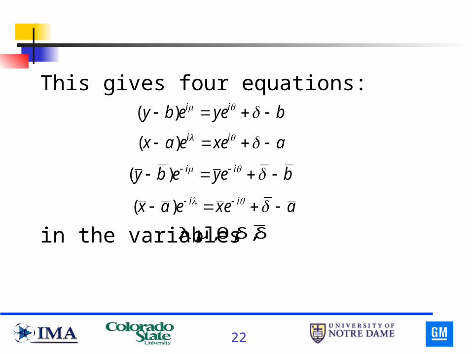
This gives four equations:
in the variables δδ,θ,μ,λ,
byeeby ii )(
axeeax ii )(
beyeby ii )(
aexeax ii )(
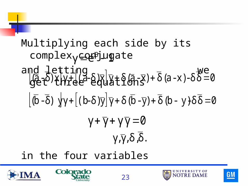
23
Multiplying each side by its complex conjugate
and letting we get three equations
in the four variables
0δ δ - x) -a ( δ )x - a( δγ x δ) -(a γx )δ - a(
0δ δ - y)- b( δ )y - b( δγ y δ) - (b γ y)δ - b(
0γ γγγ .δ δ, ,γ,γ
1eγ iθ
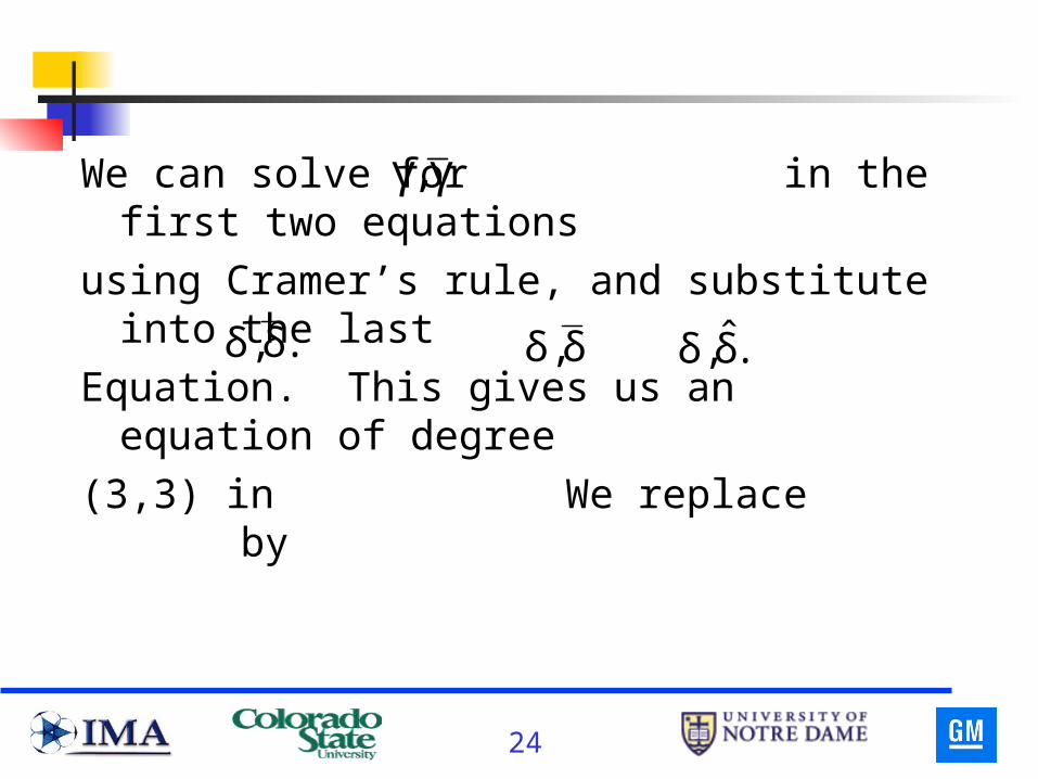
24
We can solve for in the first two equations
using Cramer’s rule, and substitute into the last
Equation. This gives us an equation of degree
(3,3) in We replace by
γ,γ
.δ δ, δ δ, .δ̂ δ,
25
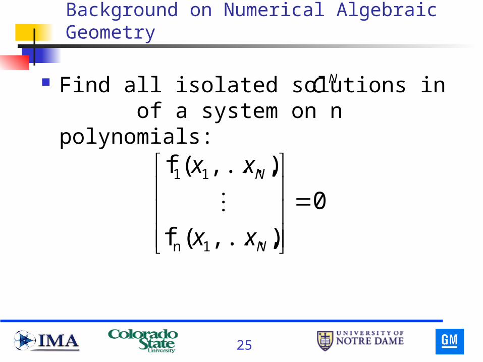
Background on Numerical Algebraic Geometry
Find all isolated solutions in of a system on n polynomials:
NC
0
),...,(f
),...,(f
1n
11
N
N
xx
xx

26
Solving a system
Homotopy continuation is our main tool: Start with known solutions of a known start
system and then track those solutions as we deform the start system into the system that we wish to solve.

27
Path Tracking
This method takes a system g(x) = 0, whose solutions
we know, and makes use of a homotopy, e.g.,
Hopefully, H(x,t) defines “nice paths” x(t) as t runs
from 1 to 0. They start at known solutions of
g(x) = 0 and end at the solutions of f(x) at t = 0.
tg(x). t)f(x)-(1 t)H(x,
28
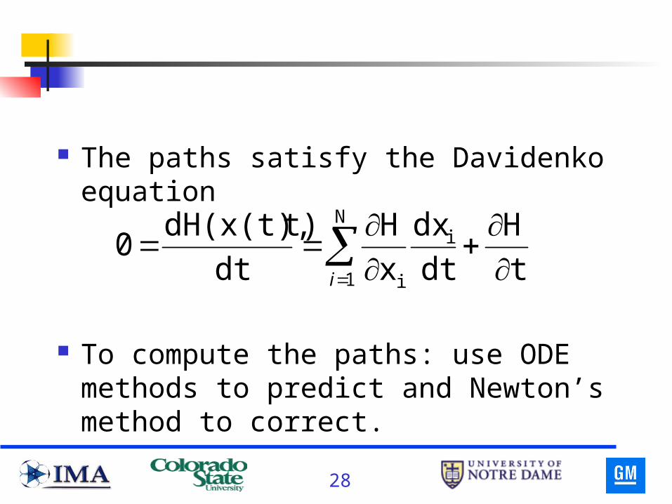
The paths satisfy the Davidenko equation
To compute the paths: use ODE methods to predict and Newton’s method to correct.
t
H
dt
dx
x
H
dt
t)dH(x(t),0
N
1
i
i
i
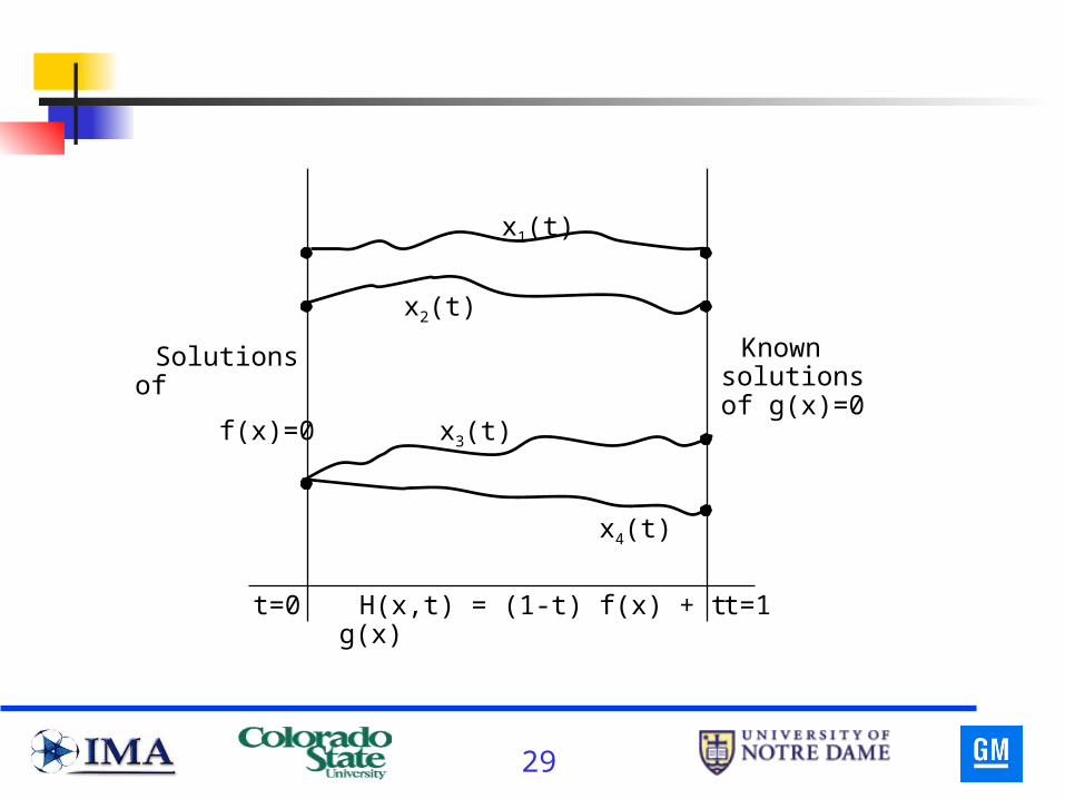
29
Solutions of
f(x)=0
Known solutions of g(x)=0
t=0 t=1H(x,t) = (1-t) f(x) + t g(x)
x3(t)
x1(t)
x2(t)
x4(t)
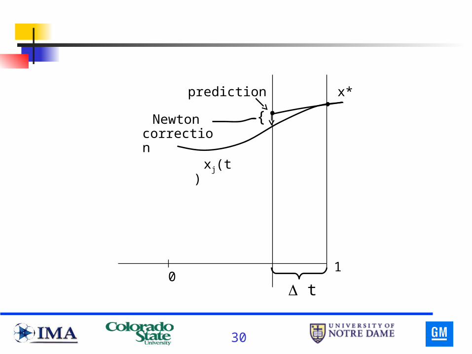
30
Newton correction
prediction
{
t
xj(t)
x*
01
31
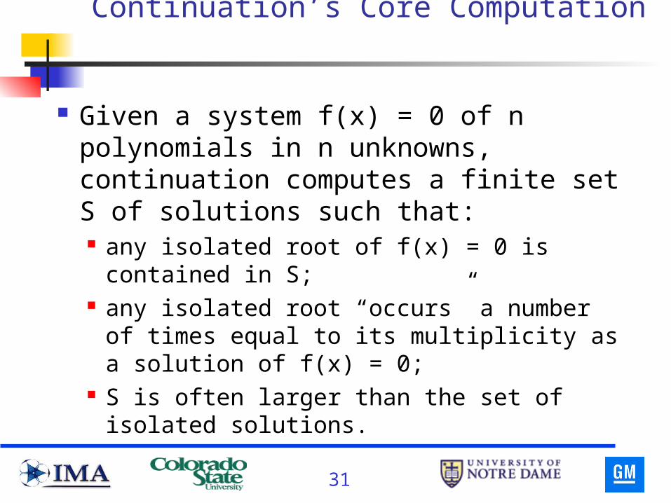
Continuation’s Core Computation
Given a system f(x) = 0 of n polynomials in n unknowns, continuation computes a finite set S of solutions such that: any isolated root of f(x) = 0 is contained in S; any isolated root “occurs” a number of times
equal to its multiplicity as a solution of f(x) = 0; S is often larger than the set of isolated
solutions.

32
Positive Dimensional Solution Sets
We now turn to finding the positive dimensional solution sets of a system
0
),...,(f
),...,(f
1n
11
N
N
xx
xx
33
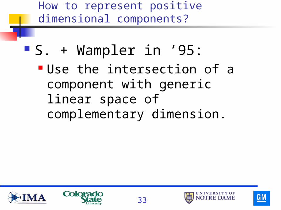
How to represent positive dimensional components?
S. + Wampler in ’95: Use the intersection of a component with
generic linear space of complementary dimension.
34
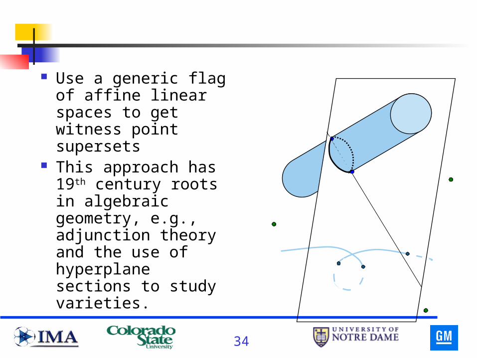
Use a generic flag of affine linear spaces to get witness point supersets
This approach has 19th century roots in algebraic geometry, e.g., adjunction theory and the use of hyperplane sections to study varieties.
35
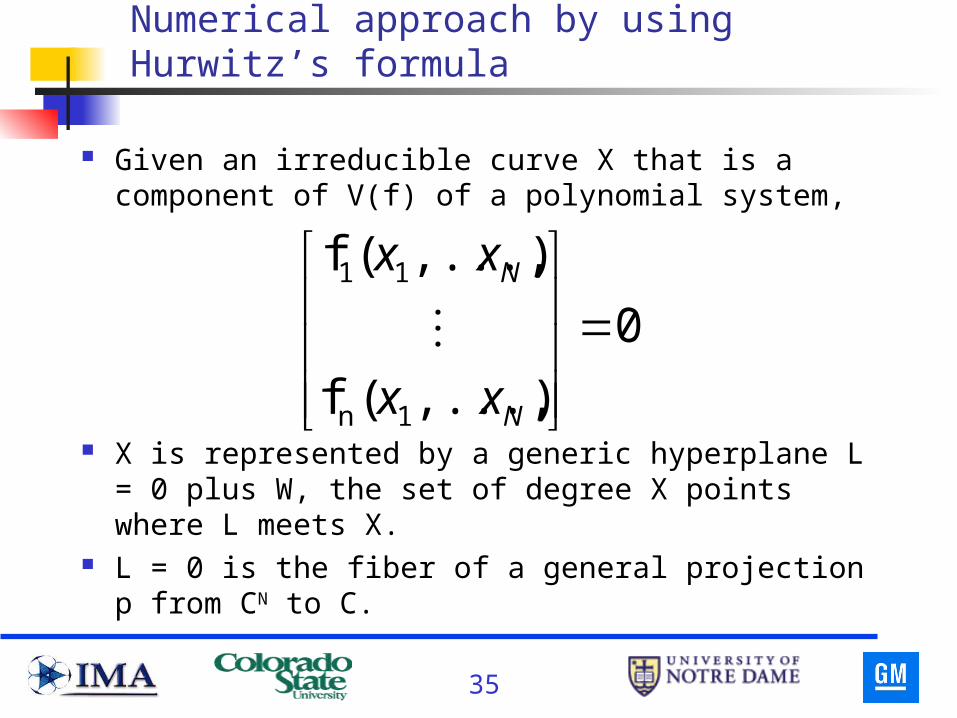
Numerical approach by using Hurwitz’s formula
Given an irreducible curve X that is a component of V(f) of a polynomial system,
X is represented by a generic hyperplane L = 0 plus W, the set of degree X points where L meets X.
L = 0 is the fiber of a general projection p from CN to C.
0
),...,(f
),...,(f
1n
11
N
N
xx
xx
36
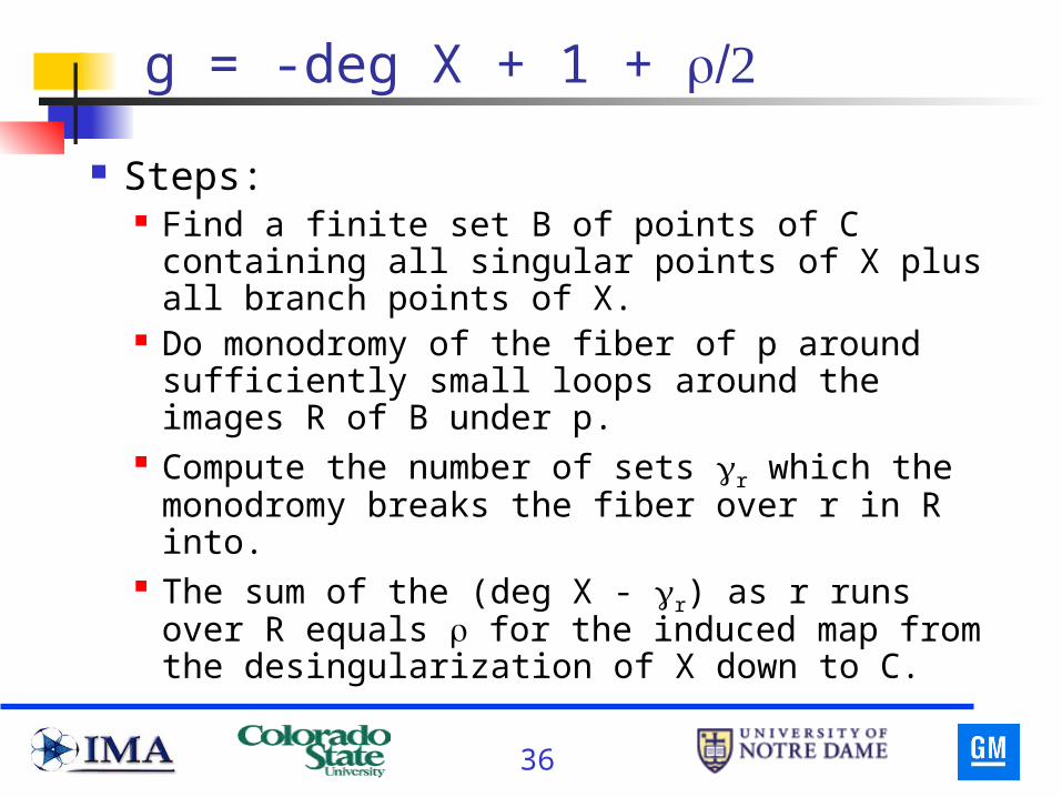
g = -deg X + 1 +
Steps: Find a finite set B of points of C containing all
singular points of X plus all branch points of X. Do monodromy of the fiber of p around
sufficiently small loops around the images R of B under p.
Compute the number of sets r which the monodromy breaks the fiber over r in R into.
The sum of the (deg X - r) as r runs over R equals for the induced map from the desingularization of X down to C.
37
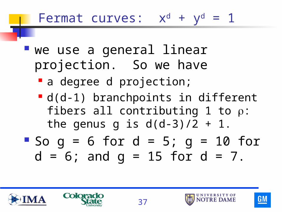
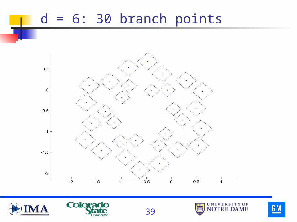
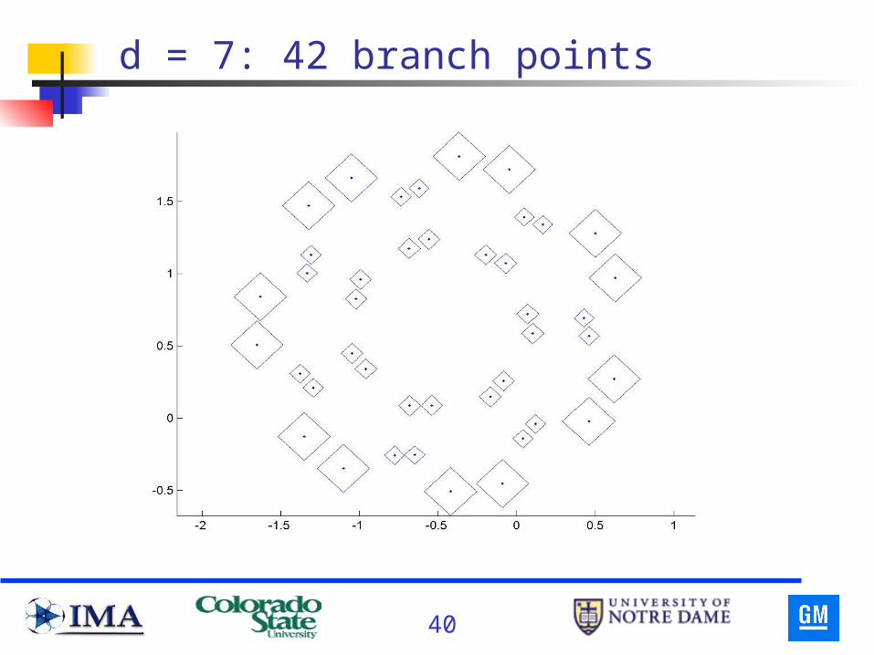
Fermat curves: xd + yd = 1
we use a general linear projection. So we have a degree d projection; d(d-1) branchpoints in different fibers all
contributing 1 to : the genus g is d(d-3)/2 + 1. So g = 6 for d = 5; g = 10 for d = 6; and g =
15 for d = 7.
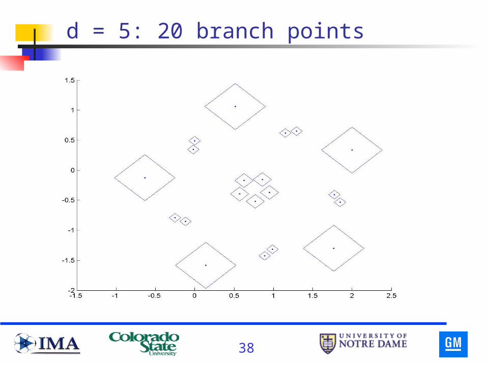
38
d = 5: 20 branch points
39
d = 6: 30 branch points
40
d = 7: 42 branch points
41
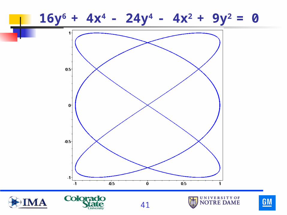
16y6 + 4x4 - 24y4 - 4x2 + 9y2 = 0
42
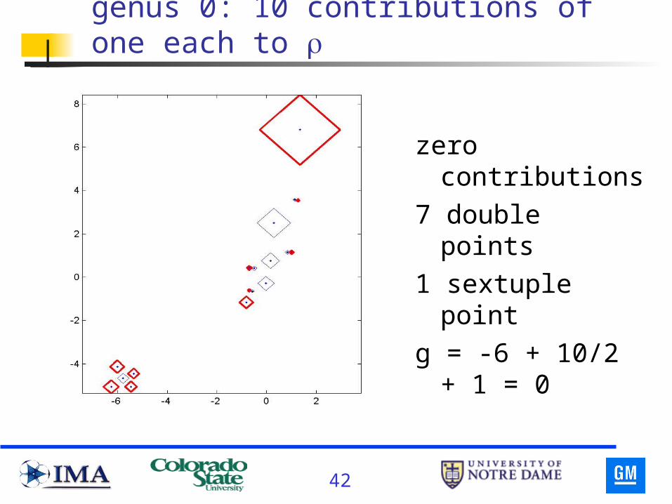
genus 0: 10 contributions of one each to
zero contributions
7 double points
1 sextuple point
g = -6 + 10/2 + 1 = 0
43
A general planar four-bar coupler curve C
C is a (3,3) curve in P1 x P1. Arithmetic genus at most 4 with at least 3 singularities: so geometric genus is at most 1.
We treat it as a degree 6 curve in P2. We compute 30 potential branch points counting multiplicities; 2 potential branch points with multiplicity 6 each make a
local contribution 0 to ; 3 potential branch points with multiplicity 2 each make a
contribution of 0 to ; 12 potential branch points contribute one each to
44
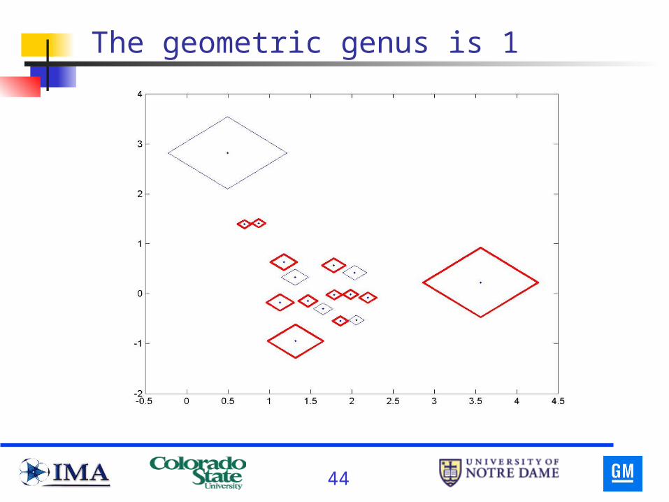
The geometric genus is 1
45
Summary
The numerical approach gives a direct method of computing the geometric genus of one-dimensional irreducible components of the solutions set of a system of polynomials.