Embed Size (px)
Citation preview

Colloidal Ordering
Under External Electric Fields
by
Ning Li
A Thesis Submitted in Partial Fulfilment of
the Requirements for the Degree of
Master of Science
Department of Physics and Physical Oceanography
Memorial University of Newfoundland
March 27, 2008
St. John’s Newfoundland
Abstract
Colloidal science is an important branch of “soft condensed matter”, which
incorporates insights from chemistry, physics and biology. In this thesis, I will
present the synthesis of fluorescently labeled core-shell silica colloids, and the
laser scanning confocal microscopy studies of these colloidal silica particles
under an external linear or rotating high-frequency alternating electric field.
The external AC field controls the averaged dipolar interaction between the
silica microspheres. We investigated bond order parameters upon increasing
the field and found the threshold of the field to form dual-particle bonds
and the average bond direction dependence on the field. We also studied
the pair correlation function of these silica colloids in external electric fields.
Moreover, we studied the equilibrium sedimentation profiles of these colloidal
suspensions and found the dependence of isothermal osmotic compressibility
on the applied electric field energy.
i

Acknowledgements
I thank my supervisor Dr. Yethiraj for his great help during our research
and my thesis correction.
I would also like to thank several others: Dr. Leunissen for her help on
Poisson Superfish software; Mr. van Kats for his generous synthesis advice;
Dr. Saika-Voivod and Dr. Agarwal for their cooperation and helpful discus-
sions in our research; Mr. Fitzgerald for our collaborative set up of electric
field simulations and gold-coated electrodes for sample cells; Mr. Newman
for collaboration in particle tracking IDL programming; Dr. Morrow, Dr.
Poduska, Dr. Merschrod, Dr. Clouter, and Mr. Gulliver for their help with
instruments; Dr. Davis (Chemistry Department Head) and Mr. Gulliver for
use of their first-year laboratory in the summer of 2006; Mr. Whelan in the
Physics Machine Shop for making the masks for gold coating; and again Dr.
Agarwal for all the photographs he took for my thesis.
ii

Contents
Abstract i
Acknowledgements ii
1 Introduction 1
1.1 Colloids . . . . . . . . . . . . . . . . . . . . . . . . . . . . . . 2
1.1.1 Definition of Colloids . . . . . . . . . . . . . . . . . . . 2
1.1.2 Forces in Colloidal Systems . . . . . . . . . . . . . . . 4
1.2 Colloids in External Electric Fields . . . . . . . . . . . . . . . 9
1.3 Experimental Methods in Colloidal Study . . . . . . . . . . . 13
2 Experimental Preparation 21
2.1 Synthesis Of Colloidal Silica Microspheres . . . . . . . . . . . 22
2.1.1 Nonfluorescent Silica Particles . . . . . . . . . . . . . . 23
2.1.2 Fluorescent-Labeled Silica Particles . . . . . . . . . . . 34
2.1.3 Seeded Growth of Core-Shell particles . . . . . . . . . . 40
2.2 Image Processing of Confocal Images Using IDL . . . . . . . . 57
iii

2.2.1 General Method for Particle Tracking . . . . . . . . . . 58
2.2.2 Structural Analysis of Colloidal System . . . . . . . . . 63
2.3 Electric Field Simulation and Construction . . . . . . . . . . . 75
2.3.1 Simulation of Electric Field . . . . . . . . . . . . . . . 75
2.3.2 Design and Construction of Electric Field Cells . . . . 83
3 Experiments, Data Analysis and Results 97
3.1 Experimental Procedures . . . . . . . . . . . . . . . . . . . . . 98
3.1.1 Sample Preparation . . . . . . . . . . . . . . . . . . . . 98
3.1.2 Experimental Setup . . . . . . . . . . . . . . . . . . . . 103
3.1.3 Experiment Procedure . . . . . . . . . . . . . . . . . . 106
3.2 Data Acquisition, Analysis and Results . . . . . . . . . . . . . 113
3.2.1 Data Acquisition . . . . . . . . . . . . . . . . . . . . . 113
3.2.2 Order Parameter Analysis and Results . . . . . . . . . 120
3.3 Conclusions . . . . . . . . . . . . . . . . . . . . . . . . . . . . 143
Outlook 147
Bibliography 149
A IDL procedures 155
B Igor Pro procedures 175
iv

List of Tables
2.1 Diameters and flow rates of peristaltic tubing . . . . . . . . . 47
2.2 Summary of centrifuge and ultrasonication conditions for dif-
ferent particle sizes . . . . . . . . . . . . . . . . . . . . . . . . 54
2.3 Summary of seeded growth . . . . . . . . . . . . . . . . . . . . 55
v

List of Figures
1.1 Schematic diagram of DLVO theory . . . . . . . . . . . . . . . 7
1.2 Dipole-dipole interactions . . . . . . . . . . . . . . . . . . . . 10
1.3 Schematic setup of confocal system . . . . . . . . . . . . . . . 15
1.4 Schematic drawing of conjugate focal pinhole . . . . . . . . . . 16
1.5 Airy disk . . . . . . . . . . . . . . . . . . . . . . . . . . . . . . 17
1.6 x-y view confocal image of core-shell silica colloids . . . . . . . 18
1.7 x-z view confocal image of core-shell silica colloids . . . . . . . 19
2.1 Ethanol distillation setup . . . . . . . . . . . . . . . . . . . . . 25
2.2 Schematic drawing of TEOS distillation setup . . . . . . . . . 27
2.3 SEM image of nonfluorescent silica particles NL0 . . . . . . . 28
2.4 SEM image and size distribution of NL1 and NL2 . . . . . . . 35
2.5 Sketches of chemicals . . . . . . . . . . . . . . . . . . . . . . . 37
2.6 Fluorescent-labeled silica seeds . . . . . . . . . . . . . . . . . . 41
2.7 Tubing setup for seeded growth . . . . . . . . . . . . . . . . . 46
2.8 Schematic drawing of seeded growth setup . . . . . . . . . . . 49
2.9 SEM images of core-shell silica particles. . . . . . . . . . . . . 53
vi
2.10 A frame from confocal image of core-shell silica particle . . . . 57
2.11 Identify Particles with IDL . . . . . . . . . . . . . . . . . . . . 61
2.12 Example of the particle number density distribution from a
three-dimensional image stack. . . . . . . . . . . . . . . . . . . 71
2.13 Completed electric field cells . . . . . . . . . . . . . . . . . . . 76
2.14 Side-view sketch of linear field electrodes. . . . . . . . . . . . . 78
2.15 Simulation result of linear field geometry. . . . . . . . . . . . . 79
2.16 Example image of an acceptable range in side-view linear field
simulation . . . . . . . . . . . . . . . . . . . . . . . . . . . . . 81
2.17 Example image of an acceptable range in top-view rotating
field simulation . . . . . . . . . . . . . . . . . . . . . . . . . . 84
2.18 The design of the linear field mask . . . . . . . . . . . . . . . 86
2.19 Brass mask for linear field. . . . . . . . . . . . . . . . . . . . . 87
2.20 The designing sketch of the rotating field mask . . . . . . . . . 89
2.21 Brass mask for rotating field. . . . . . . . . . . . . . . . . . . 90
2.22 The gold-film-electrodes coated on glass slides for two-electrode
linear field cell. . . . . . . . . . . . . . . . . . . . . . . . . . . 91
2.23 The gold-film-electrodes coated on glass slides for four-electrode
rotating field cell. . . . . . . . . . . . . . . . . . . . . . . . . . 91
2.24 Completed two-electrode linear field cell. . . . . . . . . . . . . 95
2.25 Completed four-electrode rotating field cell. . . . . . . . . . . 96
2.26 Overlap of the “wire” part of the four-electrode cell . . . . . . 96
vii
3.1 Sketch for four-electrode cell electric set up . . . . . . . . . . . 104
3.2 Z steps and bin of histogram . . . . . . . . . . . . . . . . . . . 108
3.3 Example of sedimentation profile . . . . . . . . . . . . . . . . 110
3.4 Bond density vs brightness threshold from Experiment S1 . . . 115
3.5 Features found vs volume fraction for Experiment S1 . . . . . 116
3.6 E0 vs Λ . . . . . . . . . . . . . . . . . . . . . . . . . . . . . . 119
3.7 Experiment S1: Bond density vs φ profile . . . . . . . . . . . . 120
3.8 Two bonded particles . . . . . . . . . . . . . . . . . . . . . . . 122
3.9 Experiment L1: Bond density vs volume fraction profile . . . . 124
3.10 β1 vs Λ . . . . . . . . . . . . . . . . . . . . . . . . . . . . . . . 125
3.11 Experiment S1: 〈cos2 θ〉 vs φ profile . . . . . . . . . . . . . . . 127
3.12 Bond angle parameter vs volume fraction profile for Experi-
ment L1 . . . . . . . . . . . . . . . . . . . . . . . . . . . . . . 128
3.13 α0 vs Λ . . . . . . . . . . . . . . . . . . . . . . . . . . . . . . 130
3.14 Experiment S2: α0 vs 〈E2〉 . . . . . . . . . . . . . . . . . . . . 132
3.15 g(r) vs r/σ in Experiment S1 . . . . . . . . . . . . . . . . . . . 135
3.16 g(r) vs r/σ in Experiment L1 . . . . . . . . . . . . . . . . . . 136
3.17 Pair correlation function at the first peak for Experiments S1,
S2 and L1 . . . . . . . . . . . . . . . . . . . . . . . . . . . . . 137
3.18 Experiment S1: φ vs Zp . . . . . . . . . . . . . . . . . . . . . 140
3.19 χT vs Λ . . . . . . . . . . . . . . . . . . . . . . . . . . . . . . 141
viii

Chapter 1
Introduction
In this chapter, we will introduce colloids, colloidal interaction forces and
colloidal phase behavior. We will also review the effect of external electric
fields on colloidal suspensions. Finally, the primary experimental method we
used in the work of this thesis, confocal microscopy, will be described.
1
1.1 Colloids
1.1.1 Definition of Colloids
In 1861 Thomas Graham first gave the name colloid to the substances in
an aqueous solution which could not pass through a parchment membrane
when he was studying osmosis, after the Greek κoλλα meaning glue [1]. He
deduced that the low diffusion rates of colloidal particles implied they were
fairly large, at least 1 nm in modern terms. On the other hand, the failure
of the particles to sediment implied they had an upper size limit of approx-
imately 1 µm. Fluid or solid particles in this size range dispersed in a fluid
medium are known as colloidal dispersions. Graham’s definition of the range
of colloidal particle sizes is still widely used today [2]: for example, polymer
solutions, blood cells and paint are all colloidal dispersions.
Colloidal particles normally have at least one characteristic dimension at the
length range of a few nanometers to a few micrometers, which are much larger
than the surrounding medium molecules so that the medium can be regarded
as a continuum characterized by macroscopic properties such as density, di-
electric constant and viscosity. But on the other hand, the colloidal particles
are small enough to undergo Brownian motion, a phenomenon caused by
fluctuations in the random collisions of medium molecules [1].
Use of colloids dates back to the earliest records of civilization, such as stabi-
2
lized colloidal pigments used in Stone Age cave paintings and manipulation
of colloidal systems involved in ancient pottery making [2]. In the modern
world, colloids still play an important role in science and industry. The food
industry is a typical example that uses colloid techniques, as well as the
production of paints and ceramic. Colloidal science is an important branch
of “soft condensed matter”, which incorporate subjects such as chemistry,
physics and biology. The properties of colloids that interest physicists are
their potential to invent novel materials by controlling crystallinity (such as
photonic bandgap materials) or by controlling rheological properties (such as
electrorheological fluids, which we will discuss more in the next section), as
well as their function as a model system to study condensed matter.
As a model system of condensed matter (i.e. atoms and molecules), col-
loids had been shown in the 1970’s [3] to have structures and inter-particle
forces which can be treated in the same way as in simple liquids. Therefore,
statistical mechanical concepts used in the theory of simple liquids can be
analogized to an ensemble of colloids, leading to, for example, similar equa-
tions of state when the pressure is replaced by osmotic pressure. Indeed, the
phase behavior of colloidal systems, such as freezing and melting of colloidal
crystals, shows striking resemblance to that of atomic or molecular systems.
The thermodynamic analogy can be utilized to experimentally study con-
densed matter theories [2]:� The large size of colloids (1nm - 1µm) allows for easy experimental
3

techniques to probe colloids, such as light scattering and microscopy.
But for atomic or molecular systems this is either very difficult or im-
possible.� Also due to the large size of colloids, the typical time scale for col-
loidal processes is long enough to study real-time dynamics of colloidal
particles using simple microscopy techniques.� Phase transitions can be easily achieved in colloids by changing the
particle and solvent properties, or adding an external field such as an
electric field or a magnetic field. One can easily modify inter-particle
forces in colloids; this is too difficult or perhaps impossible for atomic
or molecular systems.
1.1.2 Forces in Colloidal Systems
The forces in colloidal systems play a critical role in studies of colloidal dy-
namics and phase behavior. The simplest model is to assume all colloidal
particles are hard-sphere like, which means there is no interaction between
colloidal particles beyond their radius but there is infinitely large repulsion
between particles on contact. The phase behavior of hard-sphere colloids was
studied by Pusey and van Megen [4,5]. The only parameter that determines
the phase behavior of ideal hard-sphere particles is the volume fraction of
particles, φ. In a dilute system (φ → 0), particles are far away from each
other and behave like a dilute gas. So long as φ < 0.49, the system will be-
4
have like a fluid. If we keep increasing φ the system will show a fluid-crystal
coexistence phase for 0.49 < φ < 0.54. For φ > 0.54, the colloids behave like
a solid. The system can be compressed up to φ = 0.74 which is the maximum
volume fraction for close packing. However, Pusey and van Megen [5] also
showed that the system can be trapped in an amorphous or glass phase when
φ is larger than approximately 0.58 and well below 0.64, the volume fraction
of random close packing of spheres.
Most real colloidal systems are normally more complicated than hard spheres,
because forces other than short-range repulsion exist in colloidal systems,
which also lead to a richness in the phase behavior. A short discussion about
forces in colloidal dispersions is presented here (we only discuss the simple
case, i.e. size-monodispersed spherical particles in pure liquid or electrolyte
solution) [1, 2, 6, 7]. Forces between colloidal particles and solvent include:� Brownian force, which represents the thermal energy of molecular chaos,
has a magnitude of O(kBT/σ), where kB is Boltzmann’s constant, T
is absolute temperature, and σ is a representative length, e.g. particle
diameter (same below).� Viscous force on a particle moving at a velocity v through a medium
of viscosity η is O(ησv).
Inter-particle forces include:� The attractive van der Waals force between two colloidal particles (also
5
known as the dispersion force) may cause aggregation for colloidal par-
ticles. One can calculate the dispersion force by summing over van der
Waals forces from all pairs of molecules from different particles [8], re-
sulting in a magnitude of O(Hσ/h) at short particle separations. The
Hamaker constant H depends on the nature of the particles and the
medium in between. h is the separation between two particles.� The repulsive electrostatic double-layer forces can keep the colloidal
system stable against the dispersion force. In most cases, particularly
in polar media, colloidal particles possess an electrostatic charge due
to the dissociation of their surface groups, which will get them charged
and repulsing each other. The colloidal suspension as a whole is elec-
trically neutral, so the counterions in the solvent move onto the parti-
cles and form an electrostatic double-layer, which affects considerably
the electrostatic forces between colloidal particles. The final repulsive
electrostatic double-layer force is of a magnitude of O(Ce−κh) at short
particle separations, where C is a constant, h is the separation, and κ−1
is called the Debye-Huckel screening length (or Debye length). The De-
bye length here is normally much smaller than particle size in colloidal
systems (close to hard spheres), and can be decreased by increasing sol-
vent ionic strength (i.e. salt concentration) in colloidal dispersions. κ−1
is an important parameter indicating the “softness” of the dispersion,
about which we will show more details in 3.1.1.
6
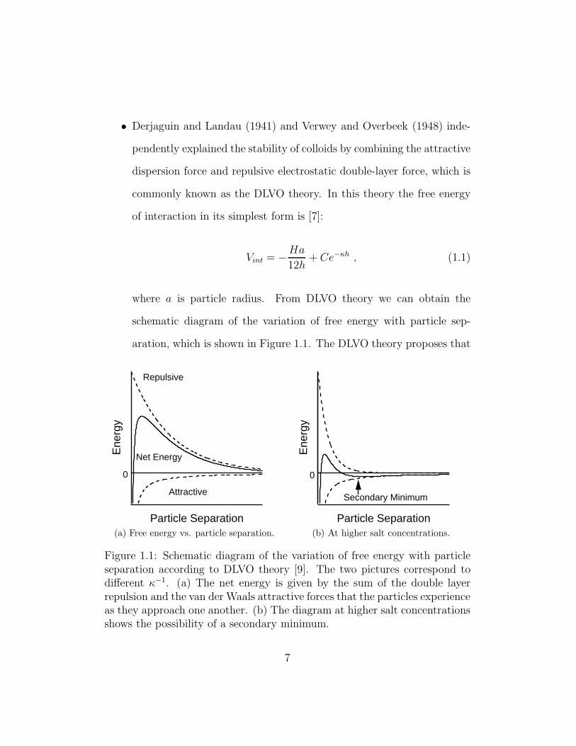
� Derjaguin and Landau (1941) and Verwey and Overbeek (1948) inde-
pendently explained the stability of colloids by combining the attractive
dispersion force and repulsive electrostatic double-layer force, which is
commonly known as the DLVO theory. In this theory the free energy
of interaction in its simplest form is [7]:
Vint = −Ha
12h+ Ce−κh , (1.1)
where a is particle radius. From DLVO theory we can obtain the
schematic diagram of the variation of free energy with particle sep-
aration, which is shown in Figure 1.1. The DLVO theory proposes that
Ene
rgy
Particle Separation
Repulsive
Net Energy
Attractive
0
(a) Free energy vs. particle separation.
Ene
rgy
Particle Separation
Secondary Minimum
0
(b) At higher salt concentrations.
Figure 1.1: Schematic diagram of the variation of free energy with particleseparation according to DLVO theory [9]. The two pictures correspond todifferent κ−1. (a) The net energy is given by the sum of the double layerrepulsion and the van der Waals attractive forces that the particles experienceas they approach one another. (b) The diagram at higher salt concentrationsshows the possibility of a secondary minimum.
7
an energy barrier resulting from the repulsive force prevents two parti-
cles from approaching one another and adhering together (Figure 1.1a).
But if the particles collide with sufficient energy to overcome that bar-
rier, the attractive force will pull them into contact where they adhere
strongly and irreversibly together. In certain situations (e.g. in high
salt concentrations), there is a possibility of a “secondary minimum”
where a much weaker and potentially reversible adhesion between par-
ticles exists (Figure 1.1b). These weak flocs are sufficiently stable not
to be broken up by Brownian motion but may dissociate under an
externally applied force such as vigorous agitation.
Besides particle-solvent interactions and inter-particle interactions, external
fields also play an important role in colloidal phase behavior. The most com-
mon external field is gravitation, which gives the effective gravitational force
(combined with buoyancy) Fg = 43πa3∆ρg for spherical colloidal particles,
where a is particle diameter and ∆ρ is density difference between particle
and surrounding fluid and g is acceleration due to gravity. Gravitational
force is negligible if the gravitational length lg = kBT/Fg is much larger than
particle diameter. But in our case it is not negligible as lg ≈ 2a (we have
lg = 1.92 µm for Experiment S1 and S2 (0.77 µm diameter spheres) and
lg = 0.59 µm for Experiment L1 (1.14 µm diameter spheres)). External elec-
tric or magnetic fields are also important methods to modify inter-particle
forces and therefore easily modify phase behaviors in colloidal systems. We
will introduce external electric fields, which are more interesting in our case,
8
in the next section.
1.2 Colloids in External Electric Fields
Colloidal particles in an external electric field whose dielectric constant is
different from that of the nonpolarizable solvent acquire an electric dipole
moment parallel to the external field [10]. The behavior of the colloids is
governed by the dipole-dipole interaction, whose strength can be tuned by
the magnitude of the field. Since their rheological properties (viscosity, yield
stress, shear modulus, etc) can be reversibly changed by the external field,
such suspensions are called electrorheological (ER) fluids. Similarly there
exists magnetorheological (MR) fluids for external magnetic fields.
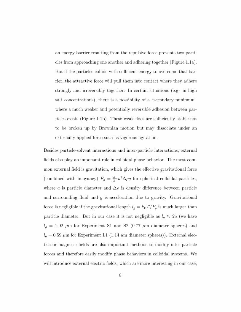
The energy of dipolar interaction shown in Figure 1.2a [10] is given by [11]
Udip(R, θ) = −4πε0εfβ2a6E2
0
R3
(
3 cos2 θ − 1
2
)
, (1.2)
where β =εp−εf
εp+2εf, εp and εf are dielectric constants for colloidal particles
and the surrounding fluid, and a is the particle radius. E20 here is the local
field energy, where ~E0, for the simplest case, is a high frequency (mega-
Hertz) sinusoidal AC field. The field frequency is so high that particles can
only see an averaged field and the effects of ion migration are minimized.
θ is the angle between separation ~R and ~E0. R here is limited to be much
9
Figure 1.2: Dipole-dipole interactions. (a) Field induced dipoles (white ar-rows) on colloidal particles with radius a interact with each other. (b) Whenfield is strong enough colloidal particles form a chain along field.
greater than particle radius, i.e. R ≫ a, given that the dipole induced by the
external field is not affected by neighboring particles, known as the point-
dipole approximation. We can see that three salient characteristics from
Equation 1.2 are:� Angular dependence. The interaction switches sign at θ0 ≈ 54.7° where
3 cos2 θ − 1 = 0. So the dipolar interaction is attractive when θ < θ0,
and repulsive when θ > θ0. This leads to head-to-toe chain formation
of colloidal particles when the field is strong enough (see Figure 1.2b).� Particle size dependence. Udip strongly depends on a as it changes as
a6.� The interaction can be tuned by external field, which provides a con-
venient method for studying phase transition in colloids as the dipo-
10
lar interaction dominates in colloids when the applied field is strong
enough.
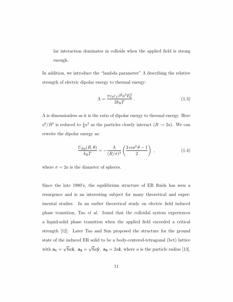
In addition, we introduce the “lambda parameter” Λ describing the relative
strength of electric dipolar energy to thermal energy:
Λ =πε0εfβ
2a3E20
2kBT. (1.3)
Λ is dimensionless as it is the ratio of dipolar energy to thermal energy. Here
a6/R3 is reduced to 18a3 as the particles closely interact (R → 2a). We can
rewrite the dipolar energy as:
Udip(R, θ)
kBT= − Λ
(R/σ)3
(
3 cos2 θ − 1
2
)
, (1.4)
where σ = 2a is the diameter of spheres.
Since the late 1980’s, the equilibrium structure of ER fluids has seen a
resurgence and is an interesting subject for many theoretical and exper-
imental studies. In an earlier theoretical study on electric field induced
phase transition, Tao et al. found that the colloidal system experiences
a liquid-solid phase transition when the applied field exceeded a critical
strength [12]. Later Tao and Sun proposed the structure for the ground
state of the induced ER solid to be a body-centered-tetragonal (bct) lattice
with a1 =√
6ax, a2 =√
6ay, a3 = 2az, where a is the particle radius [13].
11
Then Tao et al. confirmed this structure with Monte Carlo simulation [14]
and a laser diffraction experiment [15]. With the development of confocal
microscopy (which will be introduced in the next section), real-space studies
of colloidal structures became possible. The three-dimensional bct structure
of silica colloidal spheres was first observed with confocal microscopy by Das-
sanayake et al. [16].
Yethiraj et al. demonstrated the tunability of the “softness” and the dipolar
interactions of density matched colloidal dispersions by changing the salt con-
centration and external electric field, and the corresponding phase diagrams
mimicking atomic crystals [17]. The real-space access of colloidal structures
via confocal microscopy, combined with the tunability through external fields,
provides a powerful method to study colloidal phase behavior and therefore
gives better understanding of phase transitions in atomic systems such as
the melting transition [17] and the martensitic transition (i.e. a diffusionless
crystal-crystal transition) [18].
Colloids form chains along a linear external AC electric field, but will not
“crystallize” into the bct structure if the volume fraction of colloidal par-
ticles is low. The kinetics of the colloidal chain-growth at relatively high
fields (kV/cm) has been extensively studied using different methods such as
digital video microscopy [19] and light scattering [20]. However, quantitative
investigations into the low field (and low volume fraction) situation where
12

colloidal particles start to approach their nearest neighbors and form two-
particle-bond have not been done yet. Our research addresses the following
issues (see chapter 3 for detail):� Characterization of colloid structure at low electric fields (Λ > 300) and
low volume fraction (φ > 30%) with various order parameters (bond
density order parameter β1, bond orientational order parameter α0, as
well as the pair correlation function g(r)).� The feasibility of modifying colloid structure dramatically by switching
from linear to rotating electric fields� The use of gravitational sedimentation profiles to detect apparent os-
motic compressibility (χT) in almost hard-sphere-like colloids.
1.3 Experimental Methods in Colloidal Study
The techniques typically used to study colloids fall into three categories [6]:
scattering (such as x-ray, neutron and laser scattering), rheology and mi-
croscopy. Light scattering, which normally uses laser light in the visible
spectrum, is the most popular technique among scattering techniques as the
wavelength of the scattering source is close to the size of colloidal particles.
This technique accurately measures both structure and dynamics of colloidal
suspensions by averaging over large ensembles of the colloidal system, but
fails to probe details of local structure on the single particle level. The
13
rheological technique, which studies the response of the colloids to external
perturbations [21], is also not appropriate for our study because it lacks a
direct probe into short length scale structure unless incorporated with optical
techniques [22,23]. In principle, optical microscopy can be used as a probe of
local structure. But obtaining three-dimensional structure information from
conventional optical microscopy is impossible.
In order to study the local two-particle-bond formation in colloids, we used
laser scanning confocal microscopy (confocal microscopy for short), which,
when combined with refractive index matching and colloids with fluorescent
labeled core and nonfluorescent labeled shell (see chapter 2 for more detail),
has numerous advantages compared to conventional optical microscopy and
other techniques as shown below.
Better resolution
A laser scanning confocal microscope incorporates two principal ideas [6]:
point by point illumination of the sample and rejection of out of focus light.
Figure 1.3 shows a basic optical path in a typical confocal microscope: Laser
source (black line) coming out of a screen with pinhole (P1) is directed by
a dichroic mirror to two mirrors which can respectively scan in the x and
y directions. The laser then passes through the microscope objective and
excites the fluorescent sample. The frequency of fluorescent light (gray line)
emitted from sample objects is lower than that of the laser, as its photon en-
14
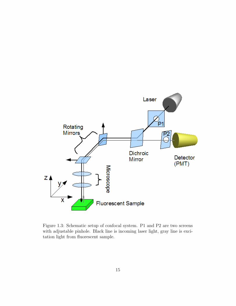
Figure 1.3: Schematic setup of confocal system. P1 and P2 are two screenswith adjustable pinhole. Black line is incoming laser light, gray line is exci-tation light from fluorescent sample.
15
ergy is lower than the absorbed photon. The emitted fluorescent light goes
back through the same path as the laser and passes the dichroic mirror as its
frequency is lower than the laser (i.e. longer wavelength). Finally, the fluo-
rescent light passes a pinhole (P2) placed in the conjugate focal (hence the
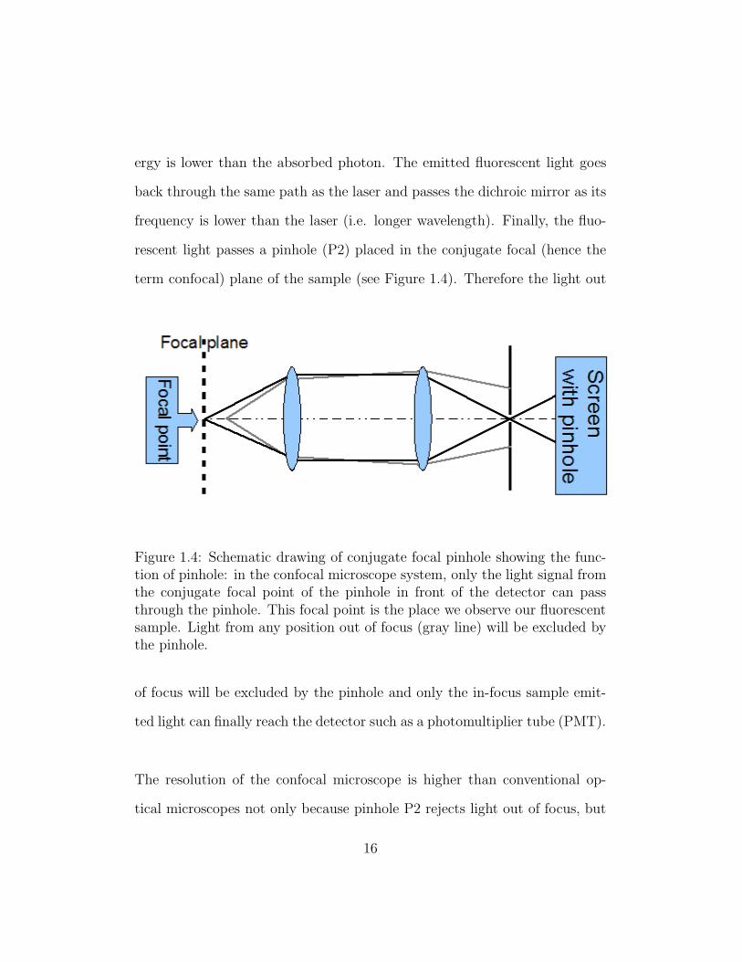
term confocal) plane of the sample (see Figure 1.4). Therefore the light out
Figure 1.4: Schematic drawing of conjugate focal pinhole showing the func-tion of pinhole: in the confocal microscope system, only the light signal fromthe conjugate focal point of the pinhole in front of the detector can passthrough the pinhole. This focal point is the place we observe our fluorescentsample. Light from any position out of focus (gray line) will be excluded bythe pinhole.
of focus will be excluded by the pinhole and only the in-focus sample emit-
ted light can finally reach the detector such as a photomultiplier tube (PMT).
The resolution of the confocal microscope is higher than conventional op-
tical microscopes not only because pinhole P2 rejects light out of focus, but
16
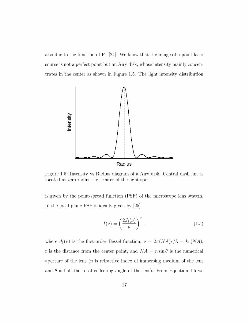
also due to the function of P1 [24]. We know that the image of a point laser
source is not a perfect point but an Airy disk, whose intensity mainly concen-
trates in the center as shown in Figure 1.5. The light intensity distributionIn
tens
ity
Radius
Figure 1.5: Intensity vs Radius diagram of a Airy disk. Central dash line islocated at zero radius, i.e. center of the light spot.
is given by the point-spread function (PSF) of the microscope lens system.
In the focal plane PSF is ideally given by [25]
I(ν) =
(
2J1(ν)
ν
)2
, (1.5)
where J1(ν) is the first-order Bessel function, ν = 2π(NA)r/λ = kr(NA),
r is the distance from the center point, and NA = n sin θ is the numerical
aperture of the lens (n is refractive index of immersing medium of the lens
and θ is half the total collecting angle of the lens). From Equation 1.5 we
17
obtain that the first minimum of intensity occurs at radius r1 = 0.61λ/NA.
Within this about 82% of the total intensity is included. On the other hand,
the distribution of excitation fluorescent light in the plane of detection is
proportional to the square of the PSF. Therefore, we use the P1 pinhole to
make our laser source close to a perfect point light source, which can greatly
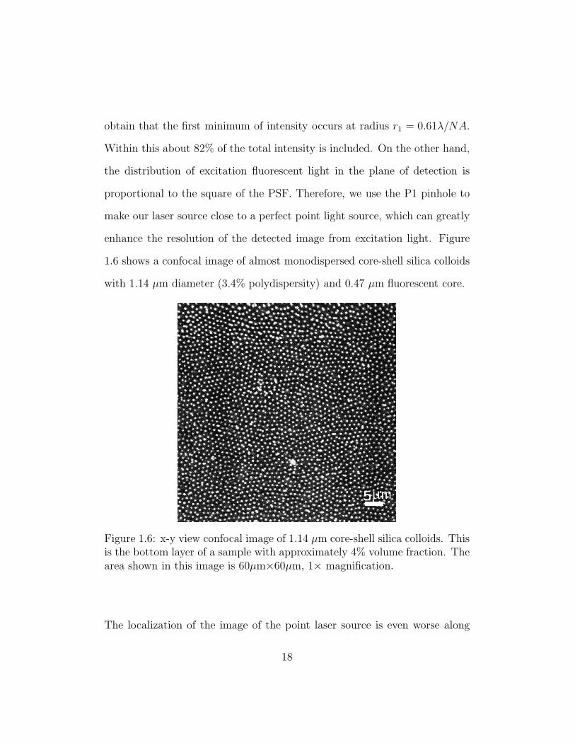
enhance the resolution of the detected image from excitation light. Figure
1.6 shows a confocal image of almost monodispersed core-shell silica colloids
with 1.14 µm diameter (3.4% polydispersity) and 0.47 µm fluorescent core.
Figure 1.6: x-y view confocal image of 1.14 µm core-shell silica colloids. Thisis the bottom layer of a sample with approximately 4% volume fraction. Thearea shown in this image is 60µm×60µm, 1× magnification.
The localization of the image of the point laser source is even worse along
18
the z direction (i.e. along the optical axis). The PSF for a plane containing
the optical axis is given by a different form:
I(u) =
(
sin(u/4)
u/4
)
, (1.6)
where u = 2π(NA)2z/(nλ) = k(NA)2z/n, z is the distance along the optical
axis. Here the first minimum is normally larger than that of the x-y plane,
which explains why we need to zoom the x dimension by a factor of 2 to get
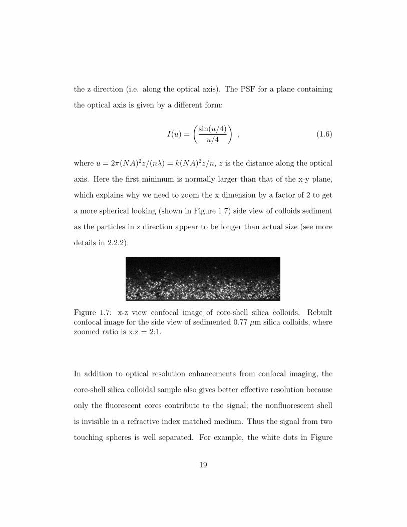
a more spherical looking (shown in Figure 1.7) side view of colloids sediment
as the particles in z direction appear to be longer than actual size (see more
details in 2.2.2).
Figure 1.7: x-z view confocal image of core-shell silica colloids. Rebuiltconfocal image for the side view of sedimented 0.77 µm silica colloids, wherezoomed ratio is x:z = 2:1.
In addition to optical resolution enhancements from confocal imaging, the
core-shell silica colloidal sample also gives better effective resolution because
only the fluorescent cores contribute to the signal; the nonfluorescent shell
is invisible in a refractive index matched medium. Thus the signal from two
touching spheres is well separated. For example, the white dots in Figure
19
1.6 are actually the fluorescent cores of touching core-shell spheres. Most of
them appear to be well separated except for a few aggregates and impurities.
Probe a sample deep inside
Conventional microscopy suffers from the multiple scattering problem which
is caused by the scattered light from objects when imaging deep into a sample.
However, a sample with the refractive index of objects (which are fluorescent
labeled) matched to that of surrounding medium can solve this problem.
Multiple scattering light is minimized and only the fluorescent light from the
labeled objects will be collected. Besides, refractive index matching can also
minimize the attractive dispersion force preventing unwanted sample aggre-
gation.
In the following chapters, we will introduce our experimental preparation
for colloidal study utilizing confocal microscopy, detailed procedures of ex-
periments and finally the results and discussion.
20
Chapter 2
Experimental Preparation
This chapter describes the experimental tools required for the confocal mi-
croscopy research presented in this thesis, including:� Section 2.1, fluorescent-nonfluorescent core-shell microspheres synthesis
for confocal microscopy samples.� Section 2.2, IDL programming for confocal image processing.� Section 2.3, electric field construction for external field applied on our
samples.
21
2.1 Synthesis Of Colloidal Silica Microspheres
This section describes the synthesis of core-shell spherical colloidal silica
particles. The synthesis followed Stober’s method [26] and Giesche condi-
tions [27, 28], and the experimental details also followed a recent M.Sc. the-
sis [29] and the work of van Blaaderen et al. [30].
This method is based on the hydrolysis of tetraethyl orthosilicate (TEOS)
and subsequent condensation of silica in an alcoholic solution of water and
ammonium hydroxide under certain reaction conditions. The silica conden-
sation forms a porous network and grows isotropically from the nuclei and
finally forms spherical particles. The core-shell particle synthesis consisted
of two stages. The first stage was the synthesis of fluorescent-labeled silica
seeds with a fluorescent dye for confocal imaging. In the second stage, a
nonfluorescent shell was grown onto these cores. A two-stage synthesis has
three advantages: the nonfluorescent shell can separate the fluorescent cores
and give a better resolution for confocal microscopy; the shell will also pro-
tect the fluorescent core and suppress the bleaching of the dye while imaging;
moreover, the growth of the shells on the fluorescent seeds can decrease the
polydispersity of the seeds.
22
2.1.1 Nonfluorescent Silica Particles
Nonfluorescent silica particles (batches name NL1, NL2, NL7, where NL
stands for Ning Li, and the numbers indicate synthesis sequence for differ-
ent batches) were prepared from TEOS in a solution of ethanol, water and
ammonium hydroxide. The reaction process is described by these two steps:
Si(OC2H5)4 + 4H2ONH3−−−−→
ethanolSi(OH)4 + 4C2H5OH (2.1)
and
Si(OH)4NH3−−−−→
ethanolSiO2 ↓ + 2H2O (2.2)
The silica condensate, which has a microscopic structure of disordered net-
works, was the spherical colloidal particles we produced.
Materials preparation
Anhydrous ethyl alcohol (Commercial Alcohols Inc., bp 78 �) was freshly
distilled before use (the general rules for the chemistry experiments we did
followed a chemistry laboratory manual [31]). We used an existing ethanol
distillation setup courtesy of Professor Morrow (Figure 2.1 shows the setup).
First some boiling stones were added to the two-neck round-bottom flask (2
Liter capacity), and then anhydrous alcohol was added to two thirds of the
whole flask volume. One of the necks was closed after adding alcohol, the
other one was connected to a water cooled distillation column, with a graded
23
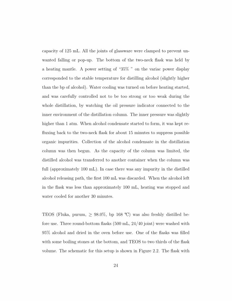
capacity of 125 mL. All the joints of glassware were clamped to prevent un-
wanted falling or pop-up. The bottom of the two-neck flask was held by
a heating mantle. A power setting of “35% ” on the variac power display
corresponded to the stable temperature for distilling alcohol (slightly higher
than the bp of alcohol). Water cooling was turned on before heating started,
and was carefully controlled not to be too strong or too weak during the
whole distillation, by watching the oil pressure indicator connected to the
inner environment of the distillation column. The inner pressure was slightly
higher than 1 atm. When alcohol condensate started to form, it was kept re-
fluxing back to the two-neck flask for about 15 minutes to suppress possible
organic impurities. Collection of the alcohol condensate in the distillation
column was then begun. As the capacity of the column was limited, the
distilled alcohol was transferred to another container when the column was
full (approximately 100 mL). In case there was any impurity in the distilled
alcohol releasing path, the first 100 mL was discarded. When the alcohol left
in the flask was less than approximately 100 mL, heating was stopped and
water cooled for another 30 minutes.
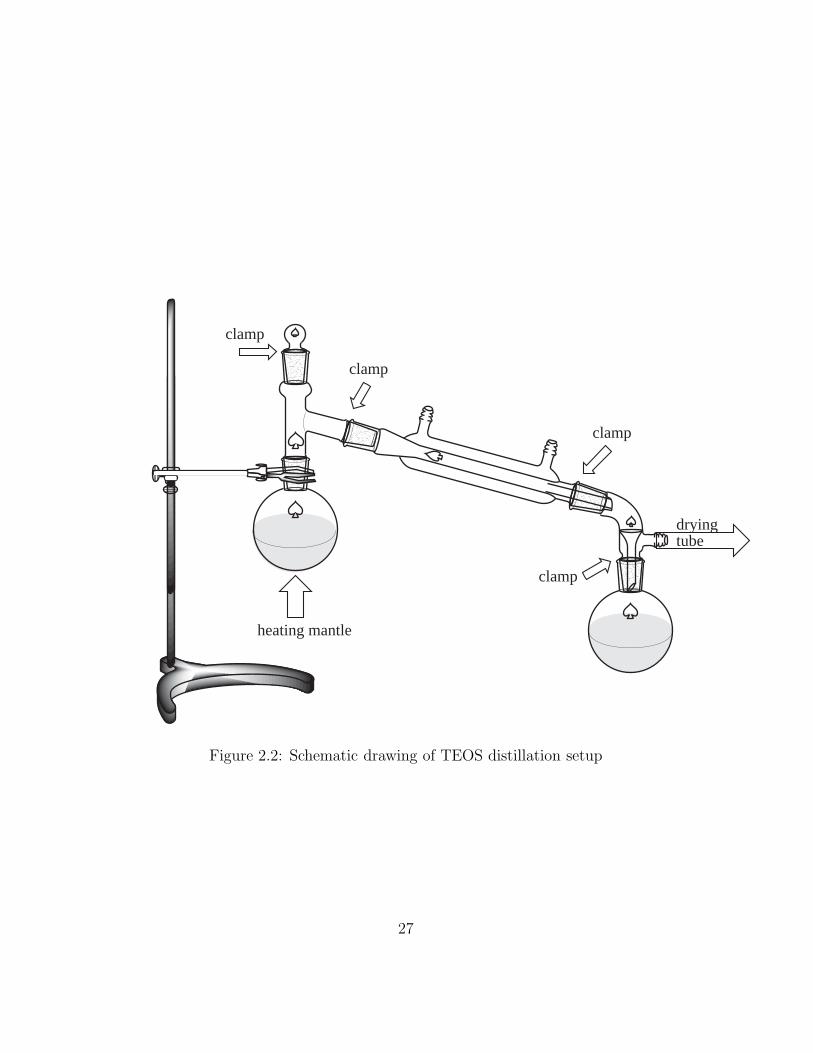
TEOS (Fluka, purum, ≥ 98.0%, bp 168 �) was also freshly distilled be-
fore use. Three round-bottom flasks (500 mL, 24/40 joint) were washed with
95% alcohol and dried in the oven before use. One of the flasks was filled
with some boiling stones at the bottom, and TEOS to two thirds of the flask
volume. The schematic for this setup is shown in Figure 2.2. The flask with
24
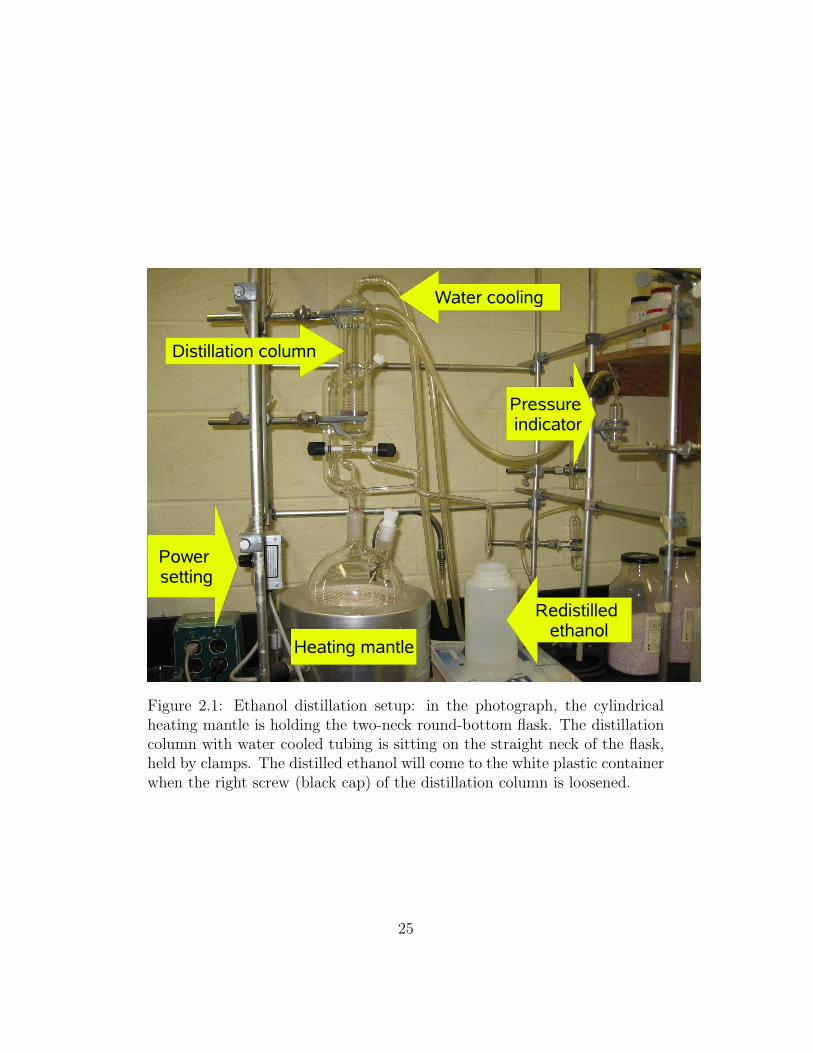
Figure 2.1: Ethanol distillation setup: in the photograph, the cylindricalheating mantle is holding the two-neck round-bottom flask. The distillationcolumn with water cooled tubing is sitting on the straight neck of the flask,held by clamps. The distilled ethanol will come to the white plastic containerwhen the right screw (black cap) of the distillation column is loosened.
25
boiling stones was held by a heating mantle and a metal lab jack. It was
connected to a condenser (air cooled) by a three-way adapter, with the other
end of the adapter closed by a stopper. The condenser was connected to a
vacuum adapter, connected to another 500 mL round-bottom flask for col-
lecting TEOS condensate, and also to a drying tube to prevent hydrolysis
of TEOS. A variable transformer (Powerstat, 3PN116C) was used as power
supply for the heating mantle, and “85” (out of “140”) on power display gave
a stable temperature for TEOS distillation (slightly higher than the bp of
TEOS). The dropping rate of condensed TEOS was about 3 drops per sec-
ond. To suppress the impurity of TEOS, the first 20 mL were discarded. All
the joints of glassware were clamped. Heating was stopped when the original
TEOS left in the first flask was less than approximately 30 mL.
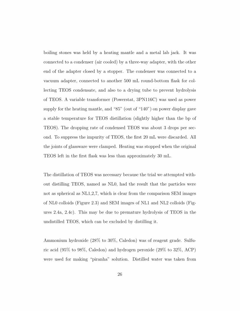
The distillation of TEOS was necessary because the trial we attempted with-
out distilling TEOS, named as NL0, had the result that the particles were
not as spherical as NL1,2,7, which is clear from the comparison SEM images
of NL0 colloids (Figure 2.3) and SEM images of NL1 and NL2 colloids (Fig-
ures 2.4a, 2.4c). This may be due to premature hydrolysis of TEOS in the
undistilled TEOS, which can be excluded by distilling it.
Ammonium hydroxide (28% to 30%, Caledon) was of reagent grade. Sulfu-
ric acid (95% to 98%, Caledon) and hydrogen peroxide (29% to 32%, ACP)
were used for making “piranha” solution. Distilled water was taken from
26
drying tube
heating mantle
clamp
clamp
clamp
clamp
Figure 2.2: Schematic drawing of TEOS distillation setup
27
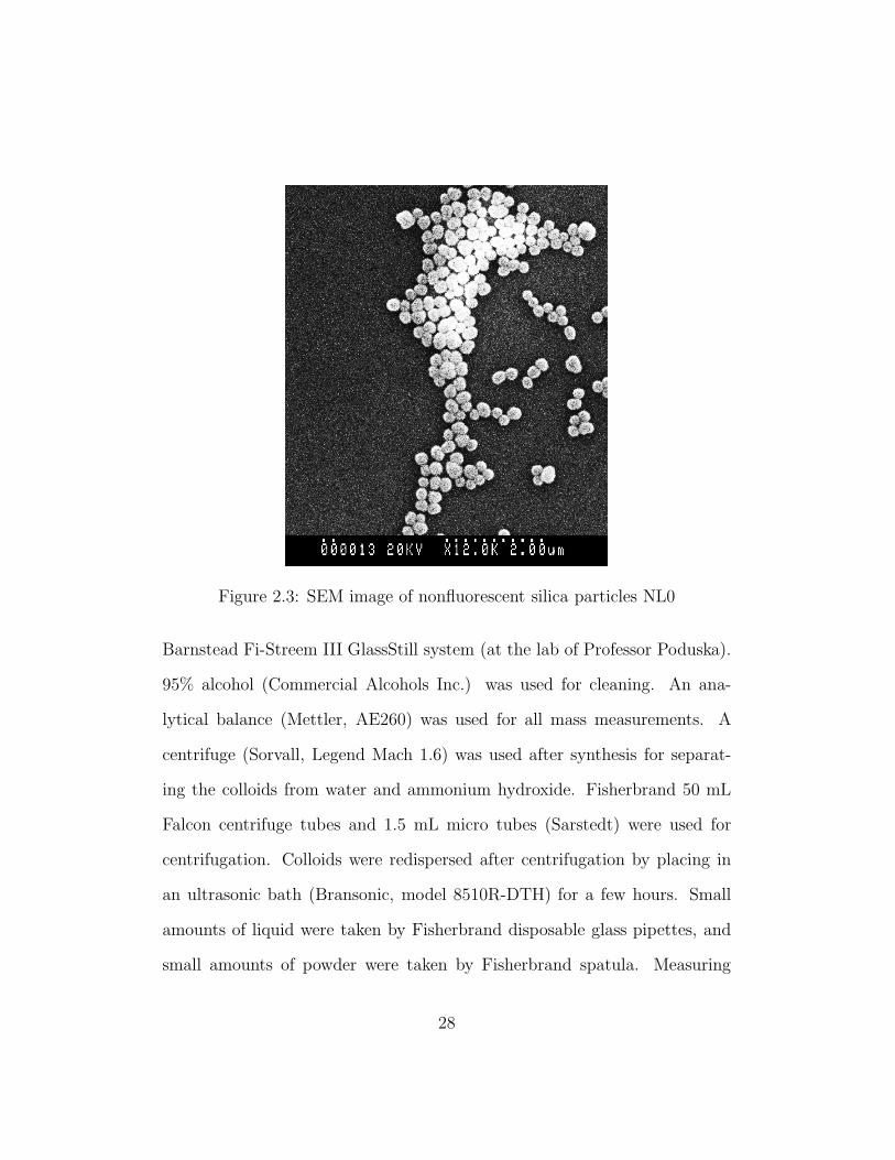
Figure 2.3: SEM image of nonfluorescent silica particles NL0
Barnstead Fi-Streem III GlassStill system (at the lab of Professor Poduska).
95% alcohol (Commercial Alcohols Inc.) was used for cleaning. An ana-
lytical balance (Mettler, AE260) was used for all mass measurements. A
centrifuge (Sorvall, Legend Mach 1.6) was used after synthesis for separat-
ing the colloids from water and ammonium hydroxide. Fisherbrand 50 mL
Falcon centrifuge tubes and 1.5 mL micro tubes (Sarstedt) were used for
centrifugation. Colloids were redispersed after centrifugation by placing in
an ultrasonic bath (Bransonic, model 8510R-DTH) for a few hours. Small
amounts of liquid were taken by Fisherbrand disposable glass pipettes, and
small amounts of powder were taken by Fisherbrand spatula. Measuring
28
small amounts of liquid was done by pipettors (Fisherbrand, finnpipette II)
and tips of same brand, or by 5 mL syringes (HSW). A Fisher Isotemp 500
Series oven was used for the drying of glassware. A hot plate stirrer (Barn-
stead Thermolyne) and a stir bar (PTFE-coated, 1 in. × 1/3 in.) was used
for stirring and heating the reaction vessel.
Equipment Preparation
A 1 L three-neck round-bottom flask, a 250 mL Erlenmeyer flask, as well
as a 50 mL and a 100 mL measuring cylinder, were used in synthesis. All
glassware (including the magnetic stir bar) was washed with piranha solution.
Face shield and thick rubber gloves must be used for protection when using
piranha solution, as it is a strong oxidizer. The piranha washing was done
in a fume hood. A 2 L beaker filled with tap water was prepared next to
the fume hood, in order to wash off any piranha solution on the gloves. To
make piranha solution, 70 ml of sulfuric acid was first added into the 100
mL measuring cylinder, then 30 ml of hydrogen peroxide was added into the
same cylinder. One should always add the peroxide into the acid, not the
other way around. The mixing reaction of peroxide and acid is exothermic,
so the mixture became very hot immediately after mixing. The hot piranha
solution was carefully transferred into the round-bottom flask. Three glass
stoppers (joint 24/40) were used to close all the openings of the flask and
held tightly with hands in case of pop-ups. The flask was slowly rotated in
ordered to wet the inside of the flask completely with piranha solution. The
29
solution was then transferred back to the 100 mL cylinder and kept in there
for a few minutes before transferring back to the flask. This procedure was
repeated three times to clean the 100 mL cylinder and 1 L flask. The same
procedure was used to clean the 50 mL cylinder and the 250 mL Erlenmeyer
flask. Once finished, the piranha solution was transferred to a glass bottle
or a beaker and neutralized with soda ash before disposing into a sink. All
glassware washed with piranha solution was rinsed with distilled water until
the pH was 7 (“Accutint” pH indicator was used). They were then rinsed
with 95% alcohol and dried in the oven.
Colloid Synthesis Setup and Procedure
The synthesis was done in the fume hood. The set up was as follows: the
middle neck of the three-neck round-bottom flask was held on the frames in
the fume hood; the stirrer was then placed under the flask. The height of
the clamp was adjusted to ensure the bottom of the flask was close to the
surface of the stirrer, so that the stir bar could smoothly stir.
Since the capacity of our reaction vessel was 1 L, the total amount of reagents
should not exceed approximately 700 mL. Therefore, the amount of reagents
were scaled down from the data in Dannis ’t Hart’s thesis [29]. 525 mL of
distilled anhydrous alcohol, 52.5 mL of ammonium hydroxide and 21 mL of
TEOS were used in this synthesis, having the total amount of 598.5 mL.
30
First, 250 mL Erlenmeyer was used to transfer 125 mL distilled alcohol into
the round-bottom flask through the right hand side opening. 52.5 mL of
ammonium hydroxide was then transferred to the flask through the same
opening by the 100 mL cylinder. Another 200 mL of alcohol was then trans-
ferred through this opening in order to rinse the ammonium hydroxide on
the wall of the flask, which otherwise may cause a high concentration of am-
monium hydroxide in that area and affect the result. After adding alcohol
and ammonium hydroxide, the stirrer was started to mix the ethanol and
ammonium hydroxide. TEOS was then added through the left hand side
opening by the 50 mL cylinder, under a vigorous stirring. This should be
done as fast as possible to suppress the hydrolysis of TEOS in the air. The
openings of the flask should be closed by the three glass stoppers during the
whole synthesis.
The reaction start time was recorded. After one minute, the stirring speed
was slowed down to a gentle stirring so that there was only a shallow vortex
at the center of the surface of solution (approximately 200 rpm). After 10
minutes the solution turned slightly milky, indicating the silica started con-
densing. Within 60 minutes, the solution turned very milky, indicating most
of the silica condensate already formed. The gentle stirring was continued
for 5 hours. The colloidal suspension was then transferred to twelve 50 mL
Falcon tubes.
31
Particle Transfer
The synthesized colloids were transferred as soon as possible to an ethanol
medium for two reasons. A high ammonium hydroxide concentration, i.e. a
high pH, gives a high ionic strength, which can decrease the thickness of the
double layer (see 1.1.2 for more details) of the particles, destroy the charge
stability and shorten the distances between particles. Although the increased
pH here, which is above the isoelectric point of silica (about 3), may cause
more surface group dissociation and finally increase the surface charge of
silica microspheres, the decreasing of the electrostatic double layer still dom-
inates and turns out to overcome the repulsive effect of the increased surface
charge. The van der Waals force between these particles, however, is only
very strong at short distances. So this force may cause irreversible aggre-
gation to the particles approaching each other at short distances. Besides,
the smell of ammonium hydroxide may cause inconvenience when working
with these colloids. Therefore, the colloidal suspension was centrifuged to
separate silica particles and the solution containing ammonium hydroxide.
An 800 rpm × 4 hours centrifugation was used for these nonfluorescent sil-
ica particles (NL1, NL2, NL7). After centrifugation, most of the particles
sedimented to the bottom and the supernatant was clear. The Falcon tubes
were then carefully taken out from the centrifuge, and kept vertical in case
the sediments redisperse to the solution. The supernatant was then removed
with glass pipettes. The tubes were then refilled with anhydrous ethanol (not
32
redistilled), and ultrasonicated in the ultrasonic bath for a few hours. Water
cooling (via a lab-made copper tube coil in the ultrasonic bath) was used
for long-time ultrasonication, as the ultrasonication heated the water in the
bath. Redispersion of colloids is more efficient if accompanied by frequent
vortexing. There is a trade off between centrifuge time and ultrasonication
time. If one use high-speed centrifugation, shorter time is needed for colloids
sedimentation, but longer time is required to redisperse by ultrasonication;
on the other hand, lower speed of centrifugation need longer time to sedi-
ment the colloids, but shorter time is required for redispersion. The exact
time and speed of centrifuge were different for different particles (see Table
2.2 for detailed centrifuge and ultrasonication time).
This centrifugation, decantation, adding fresh ethanol and redispersion pro-
cedure was repeated 3 times or more, until there was no ammonia smell in
the colloids. One can also test the pH of the colloids to ensure there is no am-
monium hydroxide left. The colloids were then transferred to a glass bottle,
and labeled by the batch name.
Polydispersity Analysis
Particle size distribution and polydispersity was obtained using scanning elec-
tron microscope (SEM) images of silica particles dried on a glass substrate.
The dried particles might appear slightly smaller on SEM than the size mea-
sured with light scattering techniques, which give the real hydrodynamic size
33
of particles. These images were analyzed using an image-processing software
ImageJ (version 1.37v) and statistics done using a graphical analysis software
Igor Pro (version 5.03). The procedure was as follows: a line was manually
drawn across the center of each particle in the SEM image to get a diam-
eter of each particle, with correct scale setting from the scale bar on the
SEM image. The diameters were recorded in a graphical analysis software
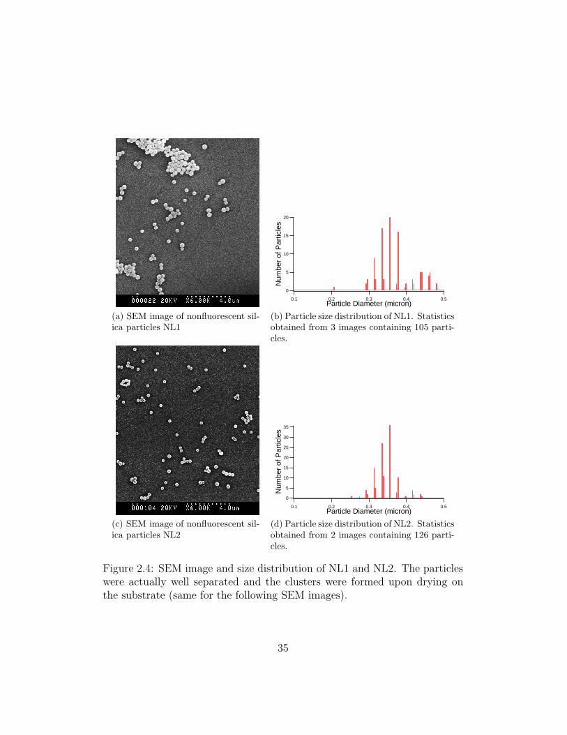
Igor Pro and the statistics were obtained. The average particle diameter of
nonfluorescent silica colloids NL1 (Figure 2.4a) was 0.37 µm, with a poly-
dispersity of 14.1% (Figure 2.4b), and NL2 (Figure 2.4c) was 0.34 µm, with
a polydispersity of 9.4% (Figure 2.4d). The SEM images and particle size
distribution of NL1 and NL2 are shown in Figure 2.4. We are not sure about
why the polydispersity of NL2 was smaller than NL1, why the particle size
distributed into two peaks and why the polydispersity was not as small as
those in the Giesche conditions (see Table 1 in [27]) which was approximately
5 to 10%, and that in the work of van Blaaderen and Vrij (approximately
5%) [30]. The possible reason could be the variance in the room temperature
for different batches of synthesis.
2.1.2 Fluorescent-Labeled Silica Particles
The purpose of fluorescent-labeling silica particles was to facilitate imaging
of confocal microscopy. The synthesis of fluorescent-labeled silica colloids
used a procedure from van Blaaderen and Vrij’s article [30]. This pro-
cedure consisted of two steps: first, the dye was chemically bonded to a
34
(a) SEM image of nonfluorescent sil-ica particles NL1
20
15
10
5
0
Num
ber
of P
artic
les
0.50.40.30.20.1Particle Diameter (micron)
(b) Particle size distribution of NL1. Statisticsobtained from 3 images containing 105 parti-cles.
(c) SEM image of nonfluorescent sil-ica particles NL2
35
30
25
20
15
10
5
0
Num
ber
of P
artic
les
0.50.40.30.20.1Particle Diameter (micron)
(d) Particle size distribution of NL2. Statisticsobtained from 2 images containing 126 parti-cles.
Figure 2.4: SEM image and size distribution of NL1 and NL2. The particleswere actually well separated and the clusters were formed upon drying onthe substrate (same for the following SEM images).
35
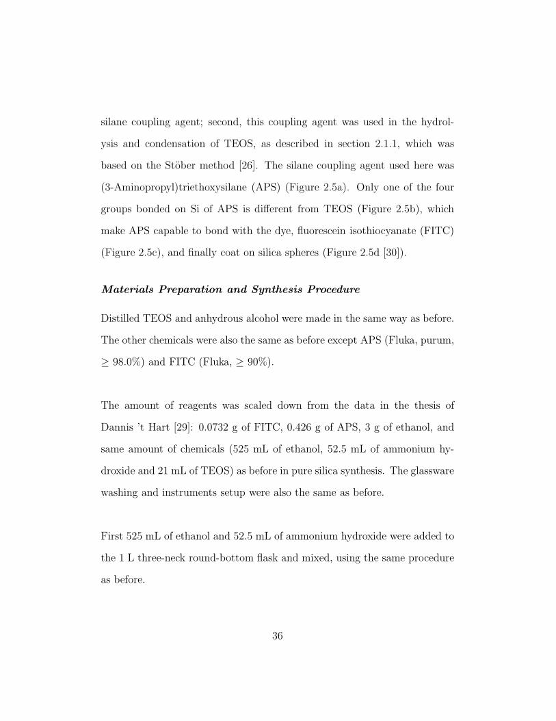
silane coupling agent; second, this coupling agent was used in the hydrol-
ysis and condensation of TEOS, as described in section 2.1.1, which was
based on the Stober method [26]. The silane coupling agent used here was
(3-Aminopropyl)triethoxysilane (APS) (Figure 2.5a). Only one of the four
groups bonded on Si of APS is different from TEOS (Figure 2.5b), which
make APS capable to bond with the dye, fluorescein isothiocyanate (FITC)
(Figure 2.5c), and finally coat on silica spheres (Figure 2.5d [30]).
Materials Preparation and Synthesis Procedure
Distilled TEOS and anhydrous alcohol were made in the same way as before.
The other chemicals were also the same as before except APS (Fluka, purum,
≥ 98.0%) and FITC (Fluka, ≥ 90%).
The amount of reagents was scaled down from the data in the thesis of
Dannis ’t Hart [29]: 0.0732 g of FITC, 0.426 g of APS, 3 g of ethanol, and
same amount of chemicals (525 mL of ethanol, 52.5 mL of ammonium hy-
droxide and 21 mL of TEOS) as before in pure silica synthesis. The glassware
washing and instruments setup were also the same as before.
First 525 mL of ethanol and 52.5 mL of ammonium hydroxide were added to
the 1 L three-neck round-bottom flask and mixed, using the same procedure
as before.
36
SiO O
O
H2N
(a) (3-Aminopropyl)triethoxysilane(APS)
Si
O
O
O
O
(b) tetraethyl orthosilicate (TEOS)
O
O
OH
O
HO
N
C
S
(c) fluorescein isothiocyanate (FITC)
O O
O OHSi
Si SiOO
O
HO
H2N(CH2)3
SiO2
(CH2)3 NH
C
S
NH
COOH
O OHO
OH
(d) FITC-APS coated on a silica sphere,from reference [30]
Figure 2.5: Sketches of chemicals
37
Then the balance and a 20 mL disposable scintillation vial and a small stir
bar (both cleaned with distilled anhydrous ethanol and dried beforehand)
were used to make the FITC-APS solution. The procedure was as follows.
First, measure the mass of the glass bottle (with stir bar in it), rezero the
balance after the display is stable. Second, take 450 µL of APS by using a
pipettor (APS density 0.946 g/mL) and add it into the bottle. Measure the
mass of the whole bottle and record the display on the balance. Since the
balance was rezeroed after measuring the bottle and the stir bar, the display
should be the mass of APS. Again rezero the balance after use. Third, add
3.8 mL distilled anhydrous ethanol (0.789 g/mL) into the bottle, measure the
mass and rezero the balance. Finally, use a spatula to add 0.0732 g of FITC
powder into the glass bottle and measure the mass. The actual masses mea-
sured for FITC powder could be slightly larger than expected, which could
help to over fluorescent-label the particles and gave better image quality for
confocal microscopy. It is important to make the FITC-APS solution as fast
as possible to suppress the possible hydrolysis of APS and bleaching of FITC,
especially the former.
Once the solution was made, the glass bottle was covered with aluminum
foil and put on a stirrer for better mixing. After approximately 15 minutes,
which was different from the stirring time in the work of van Blaaderen and
Vrij (12 hours) [30], the solution was clear and showed a dark red color.
38
21 mL distilled TEOS was then added to the round-bottom flask under vig-
orous stirring. The FITC-APS mixture was then added from the other neck
immediately. After one minute, the stirring speed was turned down to a
gentle stirring (200 rpm). The sash (covered with aluminum foil beforehand)
of the fume hood was lowered in order to suppress the bleaching of FITC.
The solution turned milky as before, but with an orange color instead of
white. After 5 hours stirring, another 3 mL of distilled TEOS and 3 mL of
distilled water were simultaneously added from two necks to coat the result-
ing particles with a thin pure silica layer, in order to protect the fluorescent
dye of the particles.
The same procedure as NL1 and NL2 was used for particle transfer. The
two batches of FITC silica seeds made by the same procedure were labeled
as NL3 and NL5.
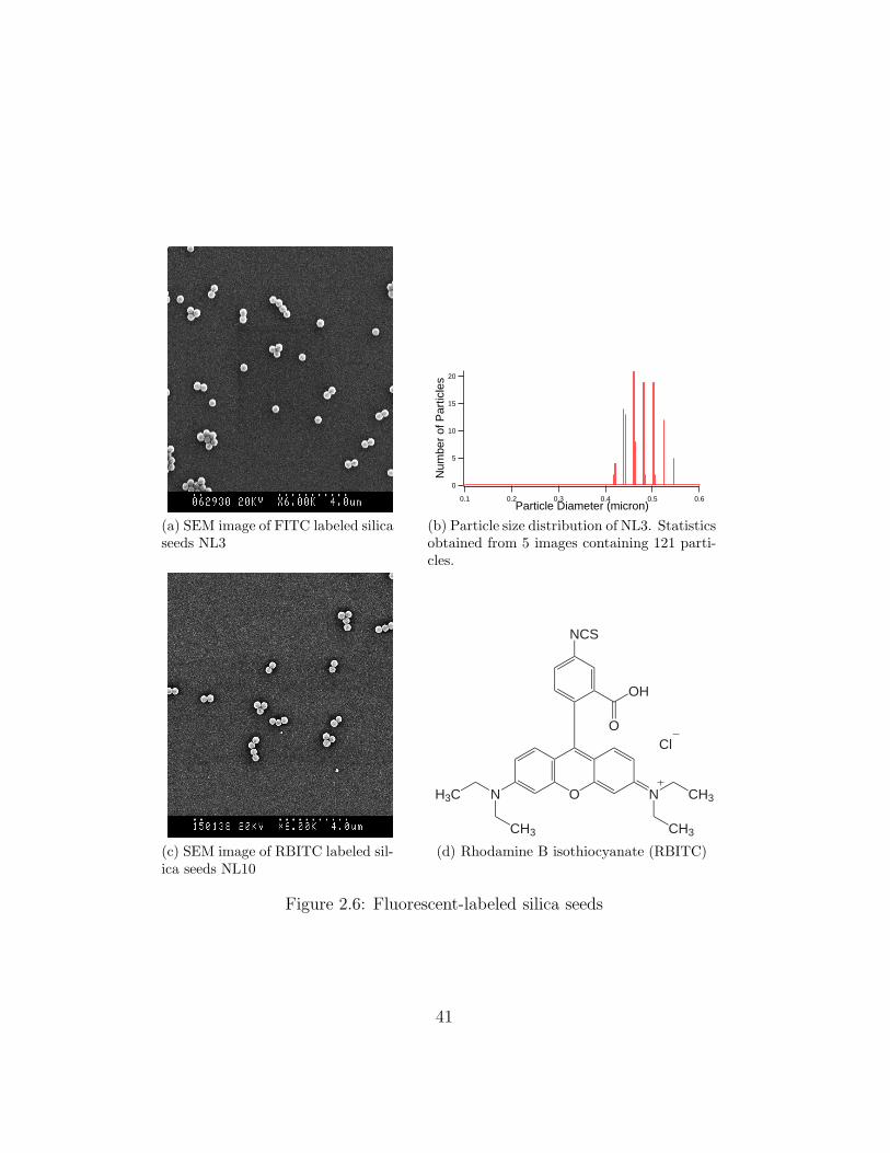
Polydispersity Analysis
Again the procedure of polydispersity analysis was the same as before. NL3
(Figure 2.6a) had a average diameter of 0.47 µm and a polydispersity of 6.9%
(Figure 2.6b). The polydispersity of NL3 was smaller than NL1 and NL2,
for as yet unknown reasons.
39
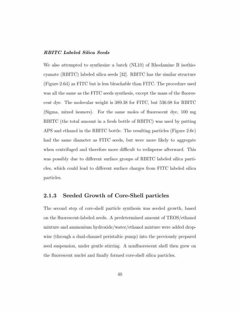
RBITC Labeled Silica Seeds
We also attempted to synthesize a batch (NL10) of Rhodamine B isothio-
cyanate (RBITC) labeled silica seeds [32]. RBITC has the similar structure
(Figure 2.6d) as FITC but is less bleachable than FITC. The procedure used
was all the same as the FITC seeds synthesis, except the mass of the fluores-
cent dye. The molecular weight is 389.38 for FITC, but 536.08 for RBITC
(Sigma, mixed isomers). For the same moles of fluorescent dye, 100 mg
RBITC (the total amount in a fresh bottle of RBITC) was used by putting
APS and ethanol in the RBITC bottle. The resulting particles (Figure 2.6c)
had the same diameter as FITC seeds, but were more likely to aggregate
when centrifuged and therefore more difficult to redisperse afterward. This
was possibly due to different surface groups of RBITC labeled silica parti-
cles, which could lead to different surface charges from FITC labeled silica
particles.
2.1.3 Seeded Growth of Core-Shell particles
The second step of core-shell particle synthesis was seeded growth, based
on the fluorescent-labeled seeds. A predetermined amount of TEOS/ethanol
mixture and ammonium hydroxide/water/ethanol mixture were added drop-
wise (through a dual-channel peristaltic pump) into the previously prepared
seed suspension, under gentle stirring. A nonfluorescent shell then grew on
the fluorescent nuclei and finally formed core-shell silica particles.
40
(a) SEM image of FITC labeled silicaseeds NL3
20
15
10
5
0
Num
ber
of P
artic
les
0.60.50.40.30.20.1Particle Diameter (micron)
(b) Particle size distribution of NL3. Statisticsobtained from 5 images containing 121 parti-cles.
(c) SEM image of RBITC labeled sil-ica seeds NL10
NCS
OH
O
ON
CH3
H3C N CH3
CH3
Cl
(d) Rhodamine B isothiocyanate (RBITC)
Figure 2.6: Fluorescent-labeled silica seeds
41
Care must be taken during the synthesis. Too low seed concentration in
suspension gives a large diffusion distance of the hydrolyzed TEOS to the
particles surface [28], which may induce premature hydrolysis and conden-
sation of TEOS, and leads to the secondary nucleation, the formation of
unwanted small silica nuclei in the seed suspension. On the other hand, too
high a seed concentration increases particle clustering, leads to unwanted
particle aggregates, which is difficult to separate from the monodisperse sus-
pension by centrifugation.
Similarly, at too low concentration of ammonium hydroxide, the particle sur-
face potential may be too low to stabilize the particles; however, too high pH
may decrease the double layer thickness, the electrostatic repulsion barrier,
and consequently reduces particle stability. So one must carefully control the
concentration of the reagents.
Giesche [28] gives empirical guidelines for optimal results (a practical guide
but not a strict limit):� the concentration of SiO2 in the seed suspension should be less than 1
M (i.e. 1 mol/L) and preferably between 0.5 and 0.8 M� the ammonium hydroxide concentration between 0.5 and 0.7 M� the water concentration about 8M
42

Materials preparation
Freshly distilled TEOS, anhydrous ethanol (not distilled, following [29]), am-
monium hydroxide and distilled water were used as before.
The seed suspension consisted of 31 mL of concentrated FITC labeled seeds
(80 g/L), 44mL ethanol, 11 mL water and 4 mL ammonium hydroxide. A
high concentration of seeds in ethanol was obtained using the procedure as
follows:� Measure the concentration of the original seeds (using the oven), esti-
mate the required amount.� Centrifuge the seeds of required amount, remove the extra ethanol and
redisperse them using ultrasonication.� Measure the concentration of these concentrated seeds to see if more
original seeds needed.� Since there will be another 44 mL ethanol in the seed suspension, one
only needs to concentrate the original seeds to a concentration of 33.07
g/L and take 75 mL of this.
When measuring the concentration, a small disposable glass vial (1 mL ca-
pacity) was first washed with 95% ethanol and dried in the oven. The mass
of the dried bottle was then measured. 500 µL of seed suspension was then
added in the bottle, dried and measured again. From the mass difference we
43
got the mass of silica per unit volume of suspension. To ensure the silica
were completely dried in the oven, the drying and measuring procedure was
repeated a few times more until there was no difference of the mass. To
minimize the error, final data was taken from the average of three batches of
measurements.
Equipment Preparation for Seeded Growth
A significant amount of equipment and optimization was required for the
seeded growth set up, and is described here.
Two cylindrical separatory funnels (capacity 500 mL, Graduated, PTFE
stopcock, 24/40 joint, Exeter), a three-neck round-bottom flask (500 mL
or 1 L, depends on the final volume of all reagents of use, 24/40 joints), and
all other glassware was washed with piranha solution using the same proce-
dure as before.
A dual-channel peristaltic pump (Gilson, minipuls3, Mandel) was used for
dropwise addition of the reagents at the same rate through two channels. The
tubing system for this pump was made following the principle that tubing
diameter should never be increased downstream. For each channel, 3 pieces
of tygon tubing (1/4 inch internal diameter (ID), 1/16 inch wall thickness;
1/8 inch ID, 1/16 wall thickness; and 1/16 inch ID, 1/32 inch wall thick-
ness, respectively) were used to assemble a long tubing whose bigger end
44
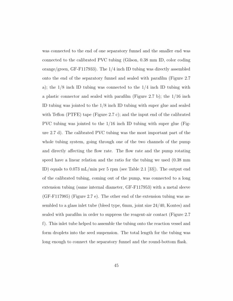
was connected to the end of one separatory funnel and the smaller end was
connected to the calibrated PVC tubing (Gilson, 0.38 mm ID, color coding
orange/green, GF-F117933). The 1/4 inch ID tubing was directly assembled
onto the end of the separatory funnel and sealed with parafilm (Figure 2.7
a); the 1/8 inch ID tubing was connected to the 1/4 inch ID tubing with
a plastic connector and sealed with parafilm (Figure 2.7 b); the 1/16 inch
ID tubing was jointed to the 1/8 inch ID tubing with super glue and sealed
with Teflon (PTFE) tape (Figure 2.7 c); and the input end of the calibrated
PVC tubing was jointed to the 1/16 inch ID tubing with super glue (Fig-
ure 2.7 d). The calibrated PVC tubing was the most important part of the
whole tubing system, going through one of the two channels of the pump
and directly affecting the flow rate. The flow rate and the pump rotating
speed have a linear relation and the ratio for the tubing we used (0.38 mm
ID) equals to 0.073 mL/min per 5 rpm (see Table 2.1 [33]). The output end
of the calibrated tubing, coming out of the pump, was connected to a long
extension tubing (same internal diameter, GF-F117953) with a metal sleeve
(GF-F117985) (Figure 2.7 e). The other end of the extension tubing was as-
sembled to a glass inlet tube (bleed type, 6mm, joint size 24/40, Kontes) and
sealed with parafilm in order to suppress the reagent-air contact (Figure 2.7
f). This inlet tube helped to assemble the tubing onto the reaction vessel and
form droplets into the seed suspension. The total length for the tubing was
long enough to connect the separatory funnel and the round-bottom flask.
45
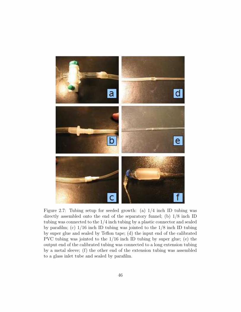
Figure 2.7: Tubing setup for seeded growth: (a) 1/4 inch ID tubing wasdirectly assembled onto the end of the separatory funnel; (b) 1/8 inch IDtubing was connected to the 1/4 inch tubing by a plastic connector and sealedby parafilm; (c) 1/16 inch ID tubing was jointed to the 1/8 inch ID tubingby super glue and sealed by Teflon tape; (d) the input end of the calibratedPVC tubing was jointed to the 1/16 inch ID tubing by super glue; (e) theoutput end of the calibrated tubing was connected to a long extension tubingby a metal sleeve; (f) the other end of the extension tubing was assembledto a glass inlet tube and sealed by parafilm.
46

Flow rate (mL/min)ID (mm) 5 rpm 15 rpm 30 rpm 48 rpm
0.38 0.073 0.219 0.436 0.695
Table 2.1: Diameters and flow rates of peristaltic tubing. The flow ratenecessary for this synthesis was 5.1 mL/h, which equals to 0.085mL/min,corresponded to a pump rotation rate of 5.82 rpm.
Seeded Growth Setup
The synthesis was carried out in the fume hood. Reagents were added as
follows:� First transfer the 90 mL of seed suspension (75 mL of seeds and ethanol,
11 mL water, 4 mL ammonium hydroxide) to the round-bottom flask.� Put the flask in a water bath (filled with tap water) on a magnetic
stirrer, and fix the flask onto the frames.� Adjust the height of the flask to get a smooth gentle stirring (approxi-
mately 200 rpm).� Fix the separatory funnels onto the frames at a proper height and
position in order to leave enough space for the tubing and flask.� Connect the tubing system to the separatory funnels, install the cal-
ibrated part onto the pump, and fix the two inlet tube onto the two
side necks of the flask (as they have the same size of joints).� Use a three-way adapter to gently blow nitrogen into the flask and keep
47

the whole reaction under a nitrogen environment, in order to suppress
the reaction between TEOS and the water vapor in the vessel.
A schematic drawing of this setup is shown as Figure 2.8. The stopper on the
center neck three-way adapter was loosened a little because of gentle flowing
of nitrogen.
Seeded Growth Procedure
Reagents were added into the separatory funnels after the seeded growth
system was installed. Aiming at a final particle size of approximately 1 µm,
the amount of TEOS needed was 159 mL following [27] and [29]. The max-
imum TEOS addition rate was 2.3 mL/h according to Giesche conditions.
Therefore, a 2 M of TEOS solution was prepared by adding 190 mL of TEOS
and 236 mL of ethanol in one separatory funnel (funnel A). A superfluous
amount of solution was added in order to leave sufficient liquid in the funnel
to keep the pump working properly during the whole seeded growth. A so-
lution of 15.4 M water and 1.35 M NH3 in ethanol was prepared by adding
100 mL of distilled water, 310 mL of ethanol and 38 mL ammonium hydrox-
ide in another separatory funnel (funnel B). The molar concentration of our
ammonium hydroxide (12.5 M), determined by titration, did not agree with
28% to 30% weight percentage (0.9 kg/L, approximately 15 M) labeled on
the bottle. So the actual molar concentration of NH3 in funnel B was 1.06
M (not 1.35 M as in [29]). This could be the possible reason that our results
did not agree with the work in [29].
48
Nitrogen
Dual-channel peristaltic pump
TE
OS/
Eth
anol
Am
mon
ia/W
ater
/Eth
anol
Room Temperature
WaterBath
Magnetic Stirrer
Figure 2.8: Schematic drawing of seeded growth setup
49
After filling with reagents, the funnels were filled with nitrogen and closed
with stoppers, in order to protect the reagents with a nitrogen environment.
The stopcocks of the two funnels were then opened and the liquid in the tub-
ing could pass through. It is sometimes necessary to squeeze the tubing in
order to exclude the air in it. Once the liquid passed through the pump (the
calibrated part of tubing), the calibrated tubings were tightened by closing
the compression cams and tightening the adjustment screws.
The cam pressure on the tubing was adjusted (by the adjustment screw)
to the minimum necessary to ensure pumping of the liquid [34]. One should
slowly tighten the screw until the pump starts pumping liquid inside the
tubing (the front of the liquid starts to flow peristaltically), and then tighten
again approximately 1/8 turn. Care must be taken not to over-tighten the
screws in order to minimize wear on the calibrated tubing.
In order to get a 2.3 mL/h TEOS adding rate, 5.1 mL/h (equals 0.085mL/min)
flow rate for TEOS solution in funnel A was used (same flow rate for funnel
B). Therefore a pump head rotating speed of 5.82 rpm was used for this
pump and this size of calibrated tubing (see Table 2.1). Since the rotating
speed was the same for the two channels, the flow rates for these two tub-
ing should be ideally the same. The hardening (by TEOS) of the calibrated
tubing, however, leaded to a different amount of flattening and stretching
50
of the calibrated tubing by the pump, thus the actual flow rates were not
the same for the two channels during the seeded growth. The longer time
the seeded growth took, the worse this problem was. Careful adjustment
of the screws was carried out after approximately 12 hours to decrease the
difference of flow rate. The flow rate difference was controlled to be within 2
mL/h during the whole seeded growth (approximately 70 hours). This is an
important area of possible improvement of particle monodispersity. Instead
of PVC calibrated tubing, one can use other more durable calibrated tubing
such as viton tubing.
The TEOS solution and ammonium hydroxide were slowly pumped through
the two channels of tubing and finally dropped into the seed suspension
through the glass tips of the inlet tube. It was important to ensure the
droplets of reagent fall in the suspension directly (especially the TEOS so-
lution) rather than fall on the wall of the vessel first. This was to avoid
locally nonuniform concentration of reagent or any hydrolysis of TEOS be-
fore it reached the seed suspension, which could cause unwanted effects like
secondary nucleation or aggregation.
Nitrogen gas was blown gently through the middle neck, preventing pre-
mature contact of the two reagent drips and unwanted hydrolysis of TEOS
with the ambient atmosphere, should be very gentle that the stopper on the
adapter can only be very slightly loosened because of the nitrogen blowing
51
out. The two separatory funnels were refilled with nitrogen approximately
every 10 hours, in order to keep the pressure balance between the inside of
outside of the funnels so that the pump can work properly.
The room temperature (outside the fume hood but in the lab), during the
whole seeded growth, was 23 �; while the water bath temperatures were 21.5� for two batches NL6 and NL8 and 19 � for NL9, without any noticeable
fluctuation. The reason for the temperature difference between the room and
water bath could be that the temperature inside the fume hood was actually
lower than outside; and the reason for the water bath temperature difference
between NL6/NL8 and NL9 may be different sizes of reaction vessels used
for these batches (NL6/NL8 1 L, NL9 500 mL).
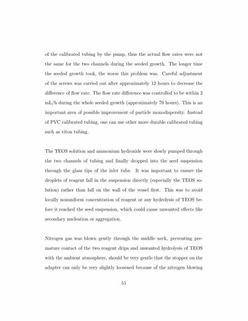
Particle Transfer and Polydispersity Analysis
The result particle transfer procedure was similar as before, using a lower
centrifuge speed of approximately 500 rpm for 4 hours. The four batches of
all seeded growth are NL4 (NL3S1, means first seeded growth of NL3 FITC
seeds), NL6 (NL3S2), NL8 (NL5S1) and NL9 (NL5S2), as shown in Figures
2.9a, 2.9b, 2.9c, and 2.9d.
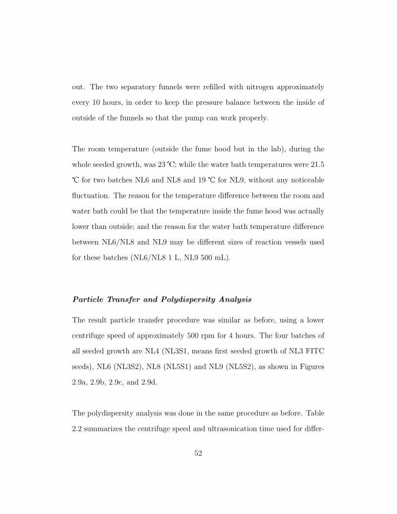
The polydispersity analysis was done in the same procedure as before. Table
2.2 summarizes the centrifuge speed and ultrasonication time used for differ-
52
(a) SEM image of NL4. Lots of non-spherical aggregates.
(b) SEM image of NL6. 1.27 µm diameter(4.1% polydispersity).
(c) SEM image of NL8. 1.14 µm diameter(3.4% polydispersity).
(d) SEM image of NL9. 0.77 µm diameter(3.8% polydispersity).
Figure 2.9: SEM images of core-shell silica particles.
53
ent batches.
Batch # � (µm) Centrifugation (rpm × hours) Ultrasonication (hours)NL1 0.37 1150 × 3 2NL2 0.34 1150 × 3 2NL3 0.47 700 × 4 6NL6 1.27 500 × 3 2NL8 1.14 500 × 3 2NL9 0.77 550 × 3 2
Table 2.2: Summary of centrifuge and ultrasonication conditions for differentparticle sizes. NL1,2,3 were centrifuged and ultrasonicated using differentcentrifuge (Sorvall) (thanks to Dr. Merschrod) and ultrasonic bath (NEY,100 Ultrasonik).
The details of the three batches of seeded growth are summarized in table
2.3. The column “funnel A” and “funnel B” refer to the amounts of TEOS
solution and ammonium hydroxide used in funnel A and B by the three
batches (keeping the same ratio of 190 mL TEOS, 236 mL ethanol for TEOS
solution and 38 mL ammonium hydroxide, 100 mL water and 310 mL ethanol
for ammonium hydroxide). The columns “NH3 (M)” / “H2O (M)” show the
start and end NH3 / H2O molar concentration in the reaction vessel. Taking
NL6 as an example: we started with the 90 mL seed suspension, contain-
ing 4 mL of ammonium hydroxide (this was the same for all three batches),
from which we can calculate that the beginning NH3 concentration in the
vessel was 0.56 M (using the titration result, i.e. 12.5 M NH3 in ammonium
hydroxide); after the synthesis was finished, 346 mL of TEOS solution and
376 mL of ammonium hydroxide had been added to the reaction vessel, from
54
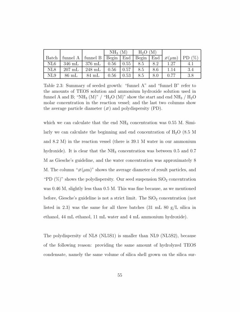
NH3 (M) H2O (M)Batch funnel A funnel B Begin End Begin End �(µm) PD (%)NL6 346 mL 376 mL 0.56 0.55 8.5 8.2 1.27 4.1NL8 207 mL 248 mL 0.56 0.57 8.5 8.6 1.14 3.4NL9 86 mL 84 mL 0.56 0.53 8.5 8.0 0.77 3.8
Table 2.3: Summary of seeded growth: “funnel A” and “funnel B” refer tothe amounts of TEOS solution and ammonium hydroxide solution used infunnel A and B; “NH3 (M)” / “H2O (M)” show the start and end NH3 / H2Omolar concentration in the reaction vessel; and the last two columns showthe average particle diameter (�) and polydispersity (PD).
which we can calculate that the end NH3 concentration was 0.55 M. Simi-
larly we can calculate the beginning and end concentration of H2O (8.5 M
and 8.2 M) in the reaction vessel (there is 39.1 M water in our ammonium
hydroxide). It is clear that the NH3 concentration was between 0.5 and 0.7
M as Giesche’s guideline, and the water concentration was approximately 8
M. The column “�(µm)” shows the average diameter of result particles, and
“PD (%)” shows the polydispersity. Our seed suspension SiO2 concentration
was 0.46 M, slightly less than 0.5 M. This was fine because, as we mentioned
before, Giesche’s guideline is not a strict limit. The SiO2 concentration (not
listed in 2.3) was the same for all three batches (31 mL 80 g/L silica in
ethanol, 44 mL ethanol, 11 mL water and 4 mL ammonium hydroxide).
The polydispersity of NL8 (NL5S1) is smaller than NL9 (NL5S2), because
of the following reason: providing the same amount of hydrolyzed TEOS
condensate, namely the same volume of silica shell grown on the silica sur-
55
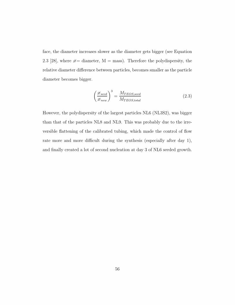
face, the diameter increases slower as the diameter gets bigger (see Equation
2.3 [28], where �= diameter, M = mass). Therefore the polydispersity, the
relative diameter difference between particles, becomes smaller as the particle
diameter becomes bigger.
(
�seed
�new
)3
=MTEOS,seed
MTEOS,total
(2.3)
However, the polydispersity of the largest particles NL6 (NL3S2), was bigger
than that of the particles NL8 and NL9. This was probably due to the irre-
versible flattening of the calibrated tubing, which made the control of flow
rate more and more difficult during the synthesis (especially after day 1),
and finally created a lot of second nucleation at day 3 of NL6 seeded growth.
56
2.2 Image Processing of Confocal Images Us-
ing IDL
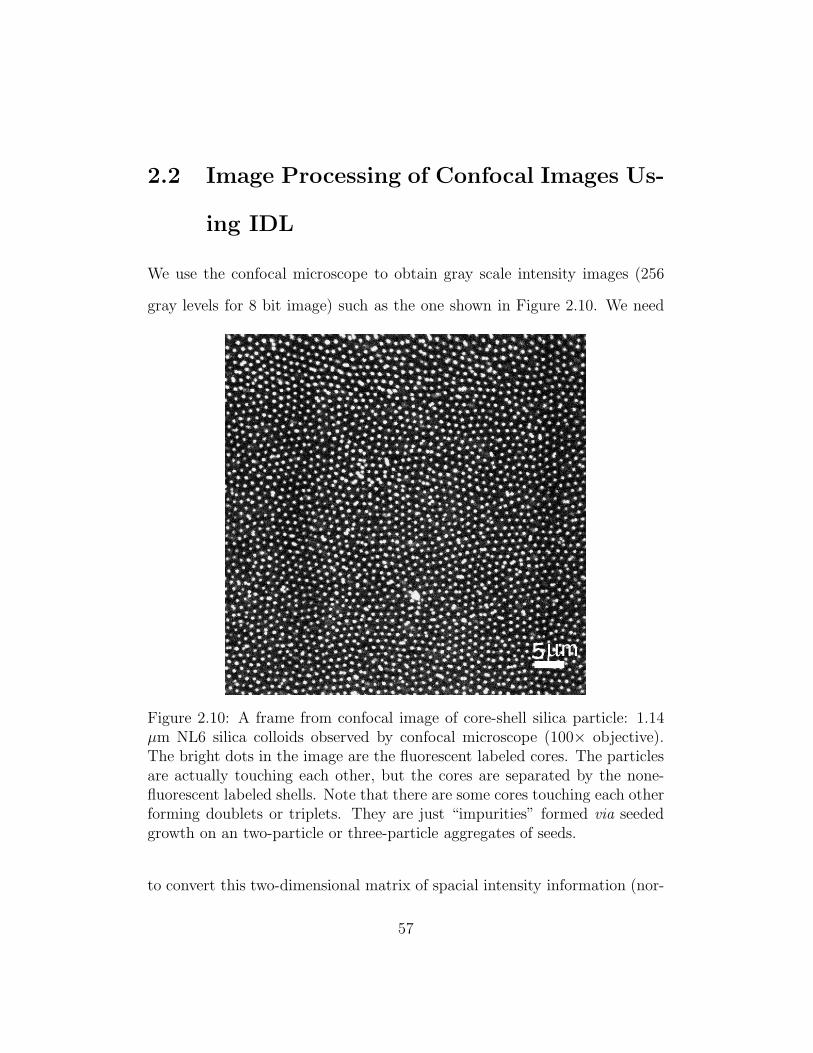
We use the confocal microscope to obtain gray scale intensity images (256
gray levels for 8 bit image) such as the one shown in Figure 2.10. We need
Figure 2.10: A frame from confocal image of core-shell silica particle: 1.14µm NL6 silica colloids observed by confocal microscope (100× objective).The bright dots in the image are the fluorescent labeled cores. The particlesare actually touching each other, but the cores are separated by the none-fluorescent labeled shells. Note that there are some cores touching each otherforming doublets or triplets. They are just “impurities” formed via seededgrowth on an two-particle or three-particle aggregates of seeds.
to convert this two-dimensional matrix of spacial intensity information (nor-
57
mally a tagged image file format, known as a “tiff” image) into information
about colloidal particles such as positions of particles. This conversion pro-
cedure for our confocal microscopy images of colloidal dispersions was done
using IDL, the Interactive Data Language. In this section, we will discuss the
methods of particle tracking and particular IDL procedures for different pur-
poses such as calculating pair correlation function, volume fraction of silica
microspheres in colloids, and order parameters of double-particle bonds.
2.2.1 General Method for Particle Tracking
The general methods of tracking bright dots on a dark background, described
in Crocker and Grier’s article [35] and the website of Eric Weeks at Emory
University [36], is suitable for our confocal images. This method normally
contains three steps: first identify particles, then get data for all the particles
you want, and finally link particles to form trajectories.
Identify Particles
IDL procedure “pretrack thresholds.pro”, based upon procedures available at
Eric Weeks’ website [36], with modifications written by Hugh Newman, was
the particle identifying procedure we used. The purpose of this procedure is
to determine the parameters we will use in particle tracking. The algorithm
of this procedure is as follows (see IDL codes in appendix A):
58
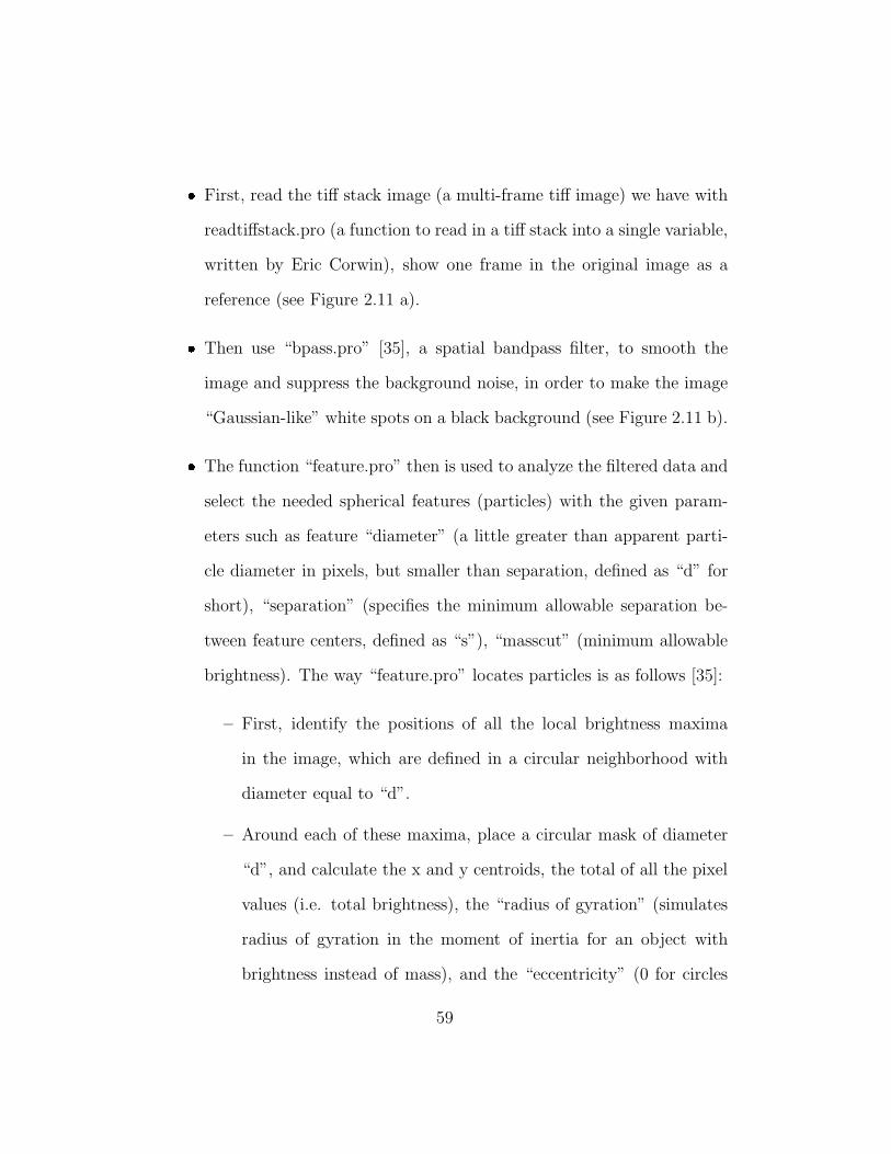
� First, read the tiff stack image (a multi-frame tiff image) we have with
readtiffstack.pro (a function to read in a tiff stack into a single variable,
written by Eric Corwin), show one frame in the original image as a
reference (see Figure 2.11 a).� Then use “bpass.pro” [35], a spatial bandpass filter, to smooth the
image and suppress the background noise, in order to make the image
“Gaussian-like” white spots on a black background (see Figure 2.11 b).� The function “feature.pro” then is used to analyze the filtered data and
select the needed spherical features (particles) with the given param-
eters such as feature “diameter” (a little greater than apparent parti-
cle diameter in pixels, but smaller than separation, defined as “d” for
short), “separation” (specifies the minimum allowable separation be-
tween feature centers, defined as “s”), “masscut” (minimum allowable
brightness). The way “feature.pro” locates particles is as follows [35]:
– First, identify the positions of all the local brightness maxima
in the image, which are defined in a circular neighborhood with
diameter equal to “d”.
– Around each of these maxima, place a circular mask of diameter
“d”, and calculate the x and y centroids, the total of all the pixel
values (i.e. total brightness), the “radius of gyration” (simulates
radius of gyration in the moment of inertia for an object with
brightness instead of mass), and the “eccentricity” (0 for circles
59
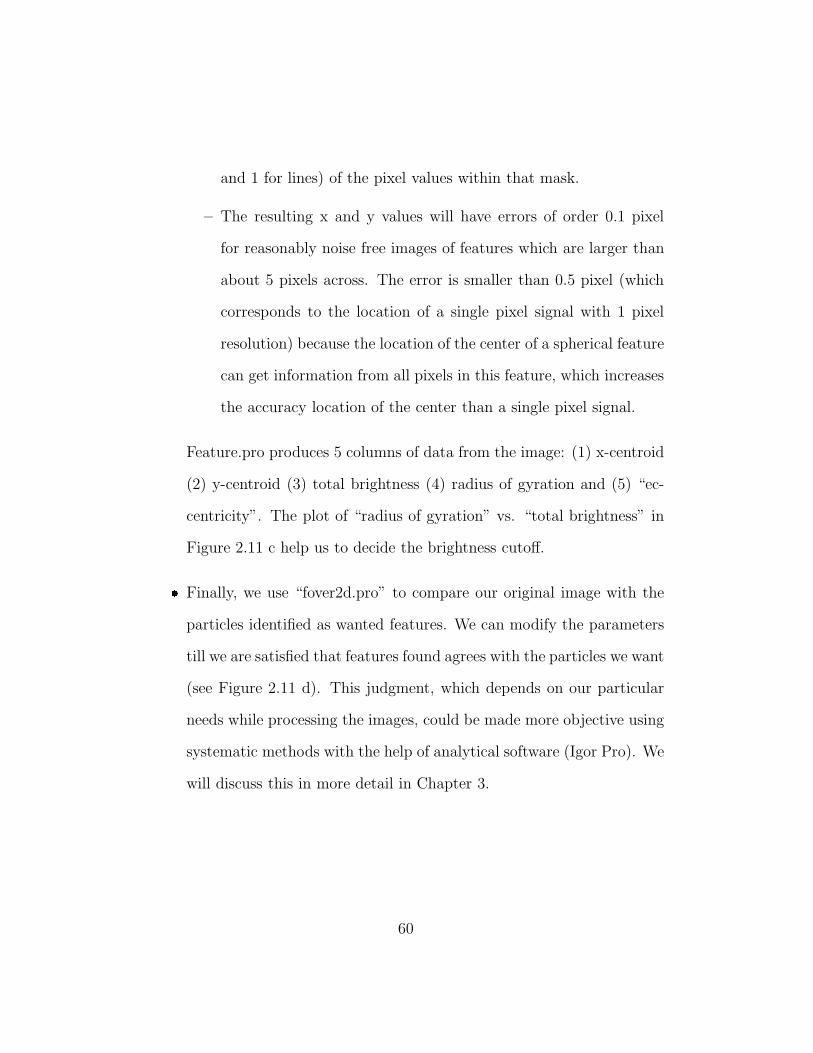
and 1 for lines) of the pixel values within that mask.
– The resulting x and y values will have errors of order 0.1 pixel
for reasonably noise free images of features which are larger than
about 5 pixels across. The error is smaller than 0.5 pixel (which
corresponds to the location of a single pixel signal with 1 pixel
resolution) because the location of the center of a spherical feature
can get information from all pixels in this feature, which increases
the accuracy location of the center than a single pixel signal.
Feature.pro produces 5 columns of data from the image: (1) x-centroid
(2) y-centroid (3) total brightness (4) radius of gyration and (5) “ec-
centricity”. The plot of “radius of gyration” vs. “total brightness” in
Figure 2.11 c help us to decide the brightness cutoff.� Finally, we use “fover2d.pro” to compare our original image with the
particles identified as wanted features. We can modify the parameters
till we are satisfied that features found agrees with the particles we want
(see Figure 2.11 d). This judgment, which depends on our particular
needs while processing the images, could be made more objective using
systematic methods with the help of analytical software (Igor Pro). We
will discuss this in more detail in Chapter 3.
60
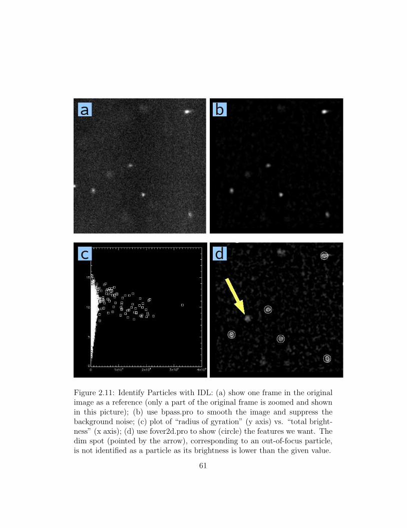
Figure 2.11: Identify Particles with IDL: (a) show one frame in the originalimage as a reference (only a part of the original frame is zoomed and shownin this picture); (b) use bpass.pro to smooth the image and suppress thebackground noise; (c) plot of “radius of gyration” (y axis) vs. “total bright-ness” (x axis); (d) use fover2d.pro to show (circle) the features we want. Thedim spot (pointed by the arrow), corresponding to an out-of-focus particle,is not identified as a particle as its brightness is lower than the given value.
61
Two-dimensional Particle Tracking
After identifying particles from a test frame, we know the parameters to find
particles in our image. We then apply these parameters to all the frames of
our stack tiff image to get the data. The procedure used here is “hpretrack-
.pro” (modified from Eric Weeks’s procedure “epretrack.pro” by Hugh New-
man with some obsolete options about Noran image format removed), which
applies the parameters to the stack tiff image and produces a gdf file (a bi-
nary file format) containing 6 columns of data. The first 5 columns are the
same as before, i.e. x and y position coordinates, brightness, etc. The 6th
column contains the uniformly gridded time “t” that the position was deter-
mined (i.e. frame number). All data in the gdf file are sorted by the frame
number so that the 6th column is monotonically increasing.
We can use the gdf file as the input of the procedure “track.pro” [35] to pro-
duce a 7-column data list. The additional 7th column is a unique “Particle
ID number” series appended to the original 6-column input data structure for
each identified particle trajectory. The result array is sorted so the rows with
corresponding ID numbers are in contiguous blocks, with the time variable
monotonically increasing inside each block. The parameters for “track.pro”
includes “maxdisp” (an estimate of the maximum pixels distance that a par-
ticle would move in a single time interval), “memory” (the maximum number
of time steps that a particle can be “lost” and then recovered again), and
“goodenough” (to eliminate all trajectories with fewer than goodenough valid
62
positions. This is useful for eliminating very short, mostly “lost” trajectories
due to blinking “noise” particles in the data stream.), etc.
Three-dimensional Particle Tracking
Particle identification and tracking in three dimensions (3D) is very similar
to two dimensions (2D) [36]. There are differences in the tools used in the 3D
procedures, for example, “bpass3d.pro” [35] is used instead of “bpass.pro”,
“feature3d.pro” [35] instead of “feature.pro” (instead of using one number for
“diameter” in 2D, we use an array containing diameter in x, y and z directions
as the “diameter” in 3D), “fover3d.pro” [35] [36] instead of “fover2d.pro”,
and “ept3d.pro” [36] instead of “hpretrack.pro”. The 3D procedure “nl -
3dpreview” (nl prefix refers to Ning Li, which means written by Ning Li) was
used to identify particles in 3D image (z-stack confocal image), similar as
“pretrack thresholds.pro” in 2D. However, “nl 3dpreview” is able to measure
the dimensions of particles in three dimensions. 3D tracking gives x, y,
and z coordinates of all particles, which can be used to study the density
distribution of silica particles in the colloidal system along z direction.
2.2.2 Structural Analysis of Colloidal System
Once we have obtained the positions of all colloidal particles in a reference
2D plane or a 3D volume, we can investigate structural information about the
colloidal system. We created IDL procedures to calculate structural quan-
tities of interest, such as the pair correlation function, the vertical particle
63
density profile, as well as two order parameters based on the bond density
and bond angle. These IDL procedures contain two parts. The first part,
discussed above, is the general method of getting the positions of all the par-
ticles we want. The second part then uses the particle positions to do our
research. We will introduce the image calibration method and algorithms of
these procedures in this subsection.
Image Calibration
Our calibration sample is a dip-coated, dried core-shell silica sample (NL9),
which has a uniform layer of 0.77 µm (about 4% uncertainty, see Table 2.3)
particles close packed. Because we can find large single domains in the dip-
coated, dried sample, we can measure the center-to-center distance along a
line of some 10 particles (thus reducing uncertainties by the same factor). We
measured the diameter in pixels of the confocal image of this sample (8.96
pixels, 2% uncertainty) so that we know it is 11.64 pixels per micron (6%
uncertainty) for a 700×700 confocal image (100× objective), corresponding
to 0.086 micron per pixel.
Pair Correlation Function
The pair correlation function g(r) calculates the probability of finding the
center of a particle a given distance from the center of another particle [36].
64
The 2D pair correlation function g(r) is defined as
g(r) =ρ(r)
ρ0
(2.4)
where
ρ(r) =n(r)
2πr · ∆r(2.5)
and
ρ0 =N
A. (2.6)
n(r)is the number of particles whose centers fall within the range of r to
r + ∆r; ∆r is a small increase in r; N is the total particle number; A is the
total area. The calculation of g(r) follows these steps:� Consider each particle in the image in turn. In the 3D case the range
is a spherical shell with thickness of ∆r, and in 2D this is an annulus
with width of ∆r. We calculate the particle number density within
this range and loop over all values of r with step size of ∆r to get the
density distribution along r. The 2D case is, for example, expressed in
equation 2.5.� Calculate the average particle number density of the whole sample,
which is the total particle number N divided by the total volume (3D)
or area (2D).
65

� Get g(r) by dividing the particle number density within r to r + ∆r
by the average particle number density, to ensure that g(r) = 1 for
structureless data (see equation 2.4).
The IDL procedure calculating 2D g(r) is “nl ericgr2d.pro” (Ning Li), apply-
ing Eric Weeks’s IDL routine “ericgr2d.pro” as part of this procedure. The
algorithm of this procedure is as follows:� Obtain 2D particle coordinates. Use the general method for 2D particle
tracking (described in 2.2.1) to get the data for all particles from a time
series of images at fixed z position.� Apply Eric Weeks’s IDL routine “ericgr2d.pro” to calculate g(r) of the
particles.
– Create 2 column matrices of identical dimensions M0 and MN ,
one (M0) where each row containing x and y coordinates of one
reference particle (x0, y0), the other (MN ) where each row contain
x and y coordinates of all the particles (N particles, for example) in
each frame of image. Subtracting MN from M0 gives all distances
(of each particle in the frame) from the reference particle, as shown
66
in Equation 2.7.
x0 y0
x0 y0
. .
. .
. .
x0 y0
−
x1 y1
x2 y2
. .
. .
. .
xN yN
=
x0 − x1 y0 − y1
x0 − x2 y0 − y2
. .
. .
. .
x0 − xN y0 − yN
(2.7)
– Compute the density function of all distances from the reference
point using “histogram” function. We decide upon the value of
the bin size of r (∆r), which is the uniform grid length of r, based
on a noise criterion. ∆r is normally much less than the particle
diameter.
– In order to get an accurate particle count using a sequence of
circular annuli of increasing radius, within a rectangular image,
we used a subroutine “checkquadrant”, which can determine how
much angular extent of the circle lies within the image when the
circle of radius r extends outside of the image.
– Divide the array of “histogram” and the array of annulus area
with radii of various r (monotonically increasing from minimum r
to maximum r by the step size of ∆r), we get the g(r) array for
this reference particle.
67
– Run this procedure by treating each the particle in the frame as
the reference in turn and loop over all frames, accumulate all the
g(r) and finally normalize it by particle number, frame number,
and average particle number density, we get the final g(r) result
for this image.� Print the result of “ericgr2d.pro”, which contains the whole range r and
corresponding g(r), into a data file readable by the graphical analysis
program Igor Pro.
Silica Colloids Vertical Density Distribution
The procedure “nl 3dhisto.pro” calculates the vertical profile of particle num-
ber density, hence we can get the vertical volume fraction distribution as a
reference parameter while doing electric field experiments.
The confocal image used for this procedure is a z-stack series (tiff file), which
is an image series taken at continuously shifting z (vertical) positions step by
step through the whole thickness of colloidal particles. The z step number
is the frame number of the z-stack series image. Along with the tiff image
stack, there is a “csv” file (text file) recording the actual z position of each z
step (i.e. each frame). The algorithm of this procedure is as follows:� Obtain 3D particle coordinates using the general method for 3D parti-
cle tracking. As the z step number in a 3D image is simply the frame
68
number, the z positions of particle centers then is expressed by a num-
ber between the minimum and maximum frame number (for example,
0 to 99 for a 100 frame z-stack image).� Obtain vertical density profile. Histogram the z positions of particle
centers to compute the particle number density distribution along z.
We wish to obtain local volume fraction as a function of z. In order
to do this, the reference volume should have thickness comparable to
the particle diameter. Therefore, the number of frames contained in
each bin of the “histogram” (defined as “binsize”) times the actual
shifted depth in each frame (defined as “stepsize”), which is the real bin
width in microns, should be slightly larger than the particle diameter
(expressed in Equation 2.8).
binsize × stepsize ≥ diameter (2.8)
That is, the “slice” has full x and y extent, and is thick enough to
include one layer of particles. We histogram the full range of z where
particles are found.� To calculate the volume fraction, multiply the volume of one particle
with the particle number in each bin, and divide by the actual volume
of that bin slice. The actual z position is from the “csv” file. The actual
x and y value is from the difference of the maximum and minimum x
and y data out of the whole image (which is very close to the full x
69

and y dimension of the image due to the densely packed particles in
the bottom frame of the image), and multiplied by 0.086 micron per
pixel, obtained from calibration.� Print output data. The output data is printed to a “dat” file, containing
one column of the z position and another column of the corresponding
number density distribution.� Moving average. Sometimes the stepsize is much smaller than particle
diameter, hence the binsize is big due to Equation 2.8. If we still need
to move in z by small steps in order to take more volume fraction data
(the reason for this is explained in the next chapter), we can simply add
another histogram of z which is shifted by a small number of frames
(“snf” for short, this number should be smaller than the binsize of the
first one), but still using the same binsize and the same maximum of
z. Then we get another set of histogram whose z position is shifted
by “snf”. By rearranging the z position in the output data, we have
a list of volume fraction with more details in terms of z position. For
example, if we set “snf” to be half of the binsize, we will then get a
series of volume fraction in the step of half bin, but with each bin width
still thick enough for the particle size.
For example, a z-stack confocal image of naturally sedimented 0.77 µm silica
particles (NL9) gives a x-z profile of the 3D cube (see Figure 2.12a), which
70
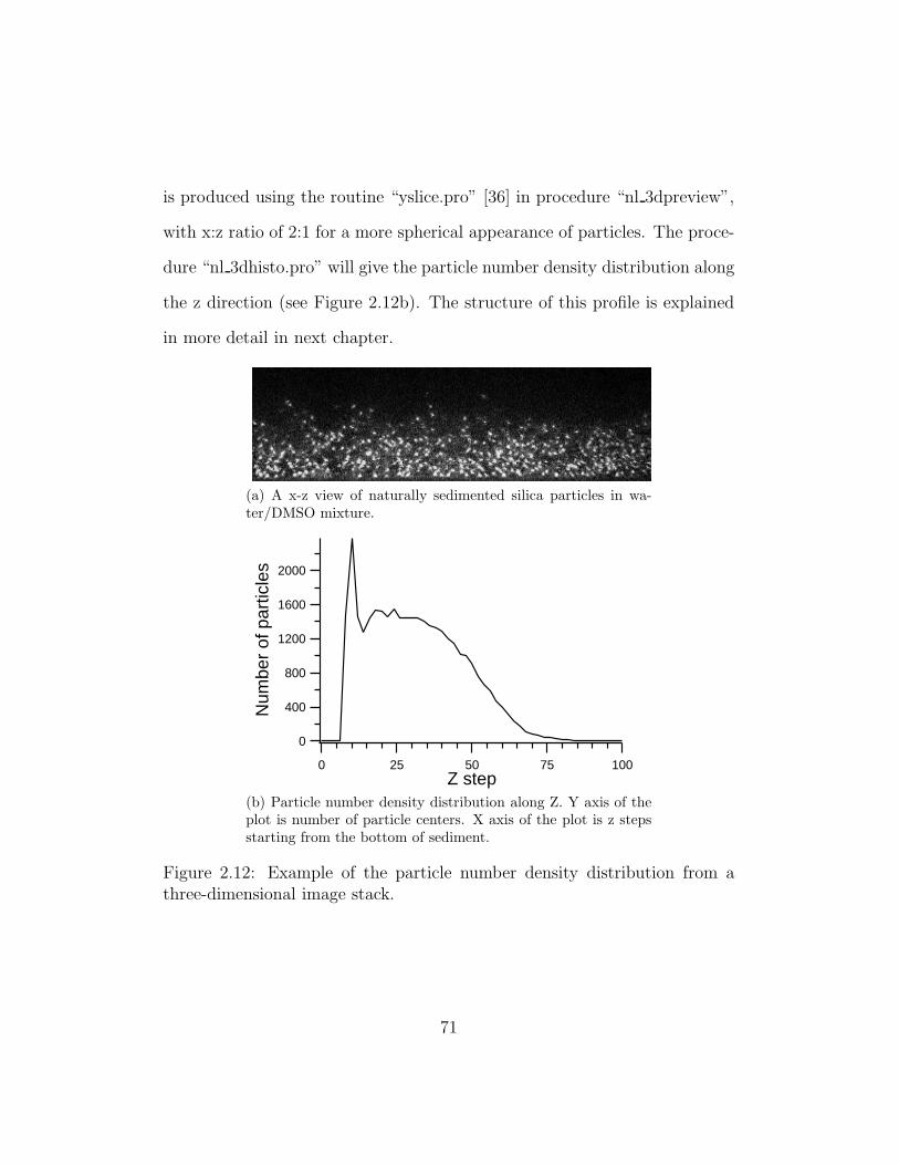
is produced using the routine “yslice.pro” [36] in procedure “nl 3dpreview”,
with x:z ratio of 2:1 for a more spherical appearance of particles. The proce-
dure “nl 3dhisto.pro” will give the particle number density distribution along
the z direction (see Figure 2.12b). The structure of this profile is explained
in more detail in next chapter.
(a) A x-z view of naturally sedimented silica particles in wa-ter/DMSO mixture.
2000
1600
1200
800
400
0
Num
ber
of p
artic
les
1007550250Z step
(b) Particle number density distribution along Z. Y axis of theplot is number of particle centers. X axis of the plot is z stepsstarting from the bottom of sediment.
Figure 2.12: Example of the particle number density distribution from athree-dimensional image stack.
71
Particle Bond Density Calculation
We define a “bond” to exist in our image when two particles are close enough
that the distance of the centers of them is shorter than the bond length we
set. Note that this bond is not a real chemical bond but simply a criterion
for describing proximity between two particles. The bond density, by our
definition, is the ratio of the number of bonded particles to the total particle
number. The procedure “nl bondensity” calculates the bond density of a
time series confocal image of our core-shell silica spheres under an external
electric field, to see how the field affects the bond density. The algorithm of
this procedure is as follows:� Obtain 2D particle coordinates.� Count number of particles in each frame. In each frame of the image, we
take the x and y coordinates of particle centers, and calculate number
of particles in the frame (represented by N). Then make a one-column
array (for the next step) with the number of rows same as the particle
number in the frame.� As the x y coordinates consist of two columns of data with the row
number equal to the number of particles found in the frame, we can
get all the possible distances (D) between each particle in the frame by
subtracting from the original coordinates a set of coordinates which are
shifted in rows by the amount of 1 to the maximum particle number
in this frame. Comparing the distances with the bond length (L), we
72
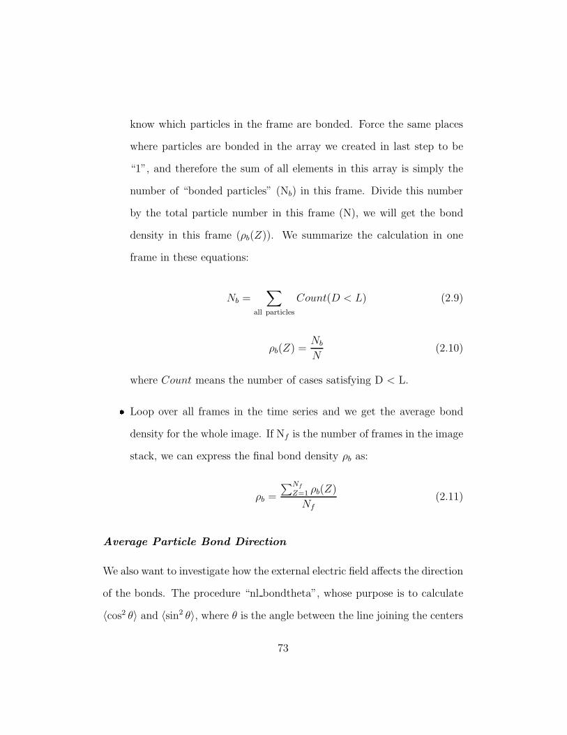
know which particles in the frame are bonded. Force the same places
where particles are bonded in the array we created in last step to be
“1”, and therefore the sum of all elements in this array is simply the
number of “bonded particles” (Nb) in this frame. Divide this number
by the total particle number in this frame (N), we will get the bond
density in this frame (ρb(Z)). We summarize the calculation in one
frame in these equations:
Nb =∑
all particles
Count(D < L) (2.9)
ρb(Z) =Nb
N(2.10)
where Count means the number of cases satisfying D < L.� Loop over all frames in the time series and we get the average bond
density for the whole image. If Nf is the number of frames in the image
stack, we can express the final bond density ρb as:
ρb =
∑Nf
Z=1 ρb(Z)
Nf
(2.11)
Average Particle Bond Direction
We also want to investigate how the external electric field affects the direction
of the bonds. The procedure “nl bondtheta”, whose purpose is to calculate
〈cos2 θ〉 and 〈sin2 θ〉, where θ is the angle between the line joining the centers
73

of two bonded particles and the external field direction along y axis, follows
this algorithm:� Obtain 2D particle coordinates.� In each frame of the image, we take the x y coordinates of particle
centers, and calculate number of particles in the frame.� Similar to the procedure for bond density (“nl bondensity”), we calcu-
late all the possible distances (D) between each particle in the frame
by shifting the coordinates in rows. Here the distances in separated x
and y direction (X and Y) are recorded as well as the total distances
between the bonded pair particles. It is actually the square of the
distances that are calculated in the procedure. To calculate cos2 θ and
sin2 θ we can simply divide the y and x distances by the total distances.� Loop over all particles in each frame and all frame of the image, we
get final 〈cos2 θ〉 and 〈sin2 θ〉. We summarize the calculation for the
complete image stack in these equations:
〈cos2 θ〉 =∑
bonded particles
Y 2/D2
Nb × Nf
(2.12)
〈sin2 θ〉 =∑
bonded particles
X2/D2
Nb × Nf
(2.13)
where Nf is the number of frames in the image stack.
74

2.3 Electric Field Simulation and Construc-
tion
The external electric field sample cells used for our colloidal systems was
designed and constructed in cooperation with Mr. Joseph Fitzgerald and
Dr. Amit Agarwal. First, we used a simulation package “Poisson Superfish”
(Los Alamos National Laboratory) to visualize and quantify the electric field
created between thin gold-film-electrodes coated on glass microscope slides
and cover slips. The purpose of the simulation was to analyze the feasibility
of using thin gold-film-electrodes on glass substrates to create a uniform
linear/rotating electric field in the plane of colloidal sample between glass
slides. Then, we used the results of the simulation to design appropriate
geometries for uniform linear and rotating fields. Finally, we constructed
electric field cells as shown in Figure 2.13.
2.3.1 Simulation of Electric Field
Simulation of Linear Field
We simulated the linear field between two pairs of thin gold-film-electrodes
on glass substrates, with solvent of various dielectric constants filling in be-
tween. Figure 2.14 shows the center part of the side-view sketch of linear
field electrodes coated on glass substrates: parts A are glass substrates (up-
per A is a cover slip, 0.17 mm thick, and bottom A is a microscope slide, 1
75
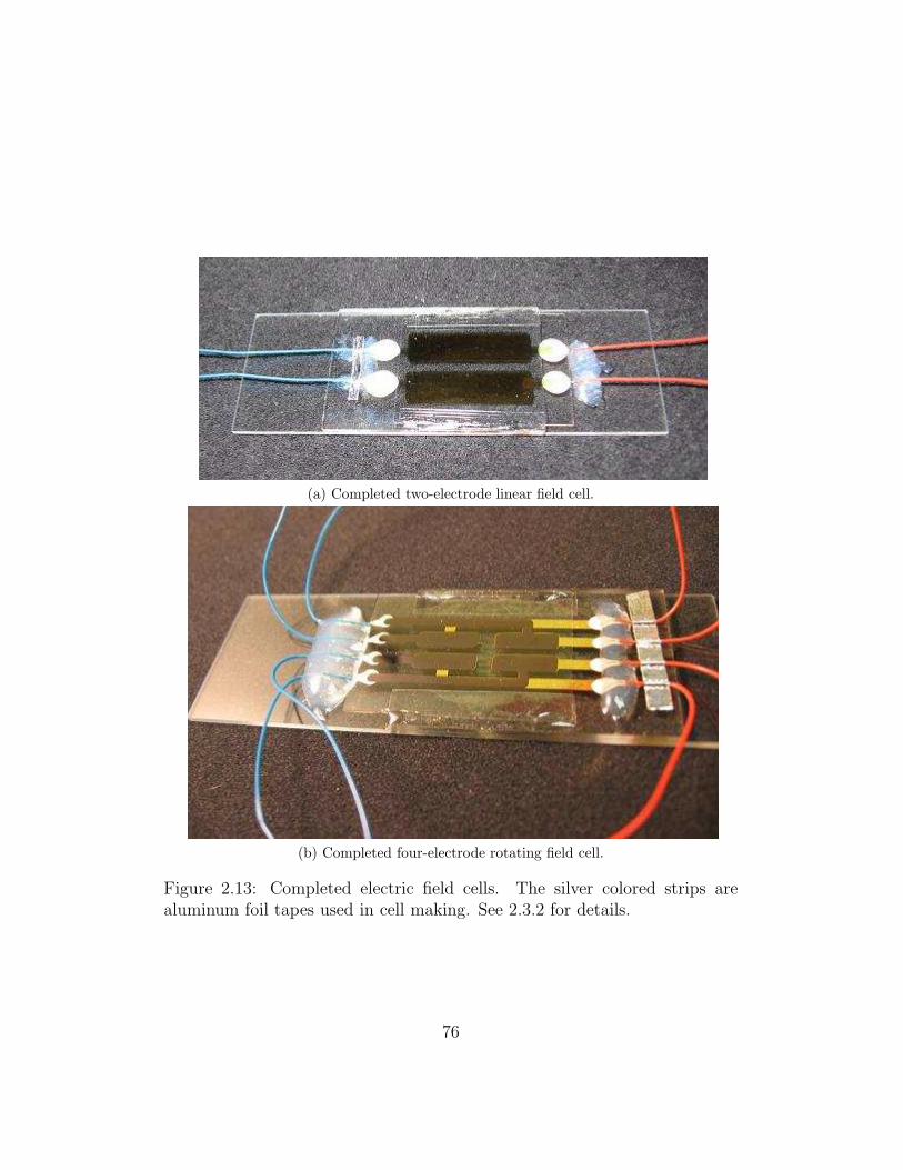
(a) Completed two-electrode linear field cell.
(b) Completed four-electrode rotating field cell.
Figure 2.13: Completed electric field cells. The silver colored strips arealuminum foil tapes used in cell making. See 2.3.2 for details.
76
mm thick); parts B are the colloidal sample we want to study, which should
be one continuous part but was most simply put into the program as three
piecewise sections; the geometric center of the part B in the middle is de-
signed to be at the center of the graph, i.e. x=0, y=0; and the two pairs of
white bars above and under the two parts B on the left and right side repre-
sent the thin gold-film-electrodes coated on glass substrates, 0.025 mm thick.
The other unmarked parts are vacuum. The geometry of the whole electric
field was first designed, an electric potential was then applied on the thin
gold-film-electrodes in the simulation (for example, the left pair was given
a potential of 200 V and the right pair was given -200 V), and the electric
field and potential in this geometry were calculated automatically (only for
the points from the intersections of the tiny triangular grid of lines in the
background, known as “mesh” in Poisson Superfish, which should be small
enough, 0.025 mm in our case, for Poisson Superfish to calculate the potential
and field correctly). Different materials were represented in the simulation
by different dielectric constants in the editable input file: 4 for glass, 80 for
water, etc.
Figure 2.15 shows the calculated electric potential and field directions of
linear field geometry. The small arrows show the direction of local electric
field, and the pine lines are equal potential lines. When moving the mouse
cursor on this graph, local position, electric field and potential are automat-
ically shown by the software.
77
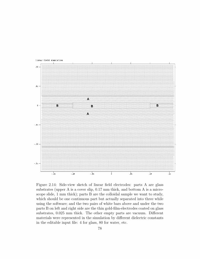
Figure 2.14: Side-view sketch of linear field electrodes: parts A are glasssubstrates (upper A is a cover slip, 0.17 mm thick, and bottom A is a micro-scope slide, 1 mm thick); parts B are the colloidal sample we want to study,which should be one continuous part but actually separated into three whileusing the software; and the two pairs of white bars above and under the twoparts B on left and right side are the thin gold-film-electrodes coated on glasssubstrates, 0.025 mm thick. The other empty parts are vacuum. Differentmaterials were represented in the simulation by different dielectric constantsin the editable input file: 4 for glass, 80 for water, etc.
78
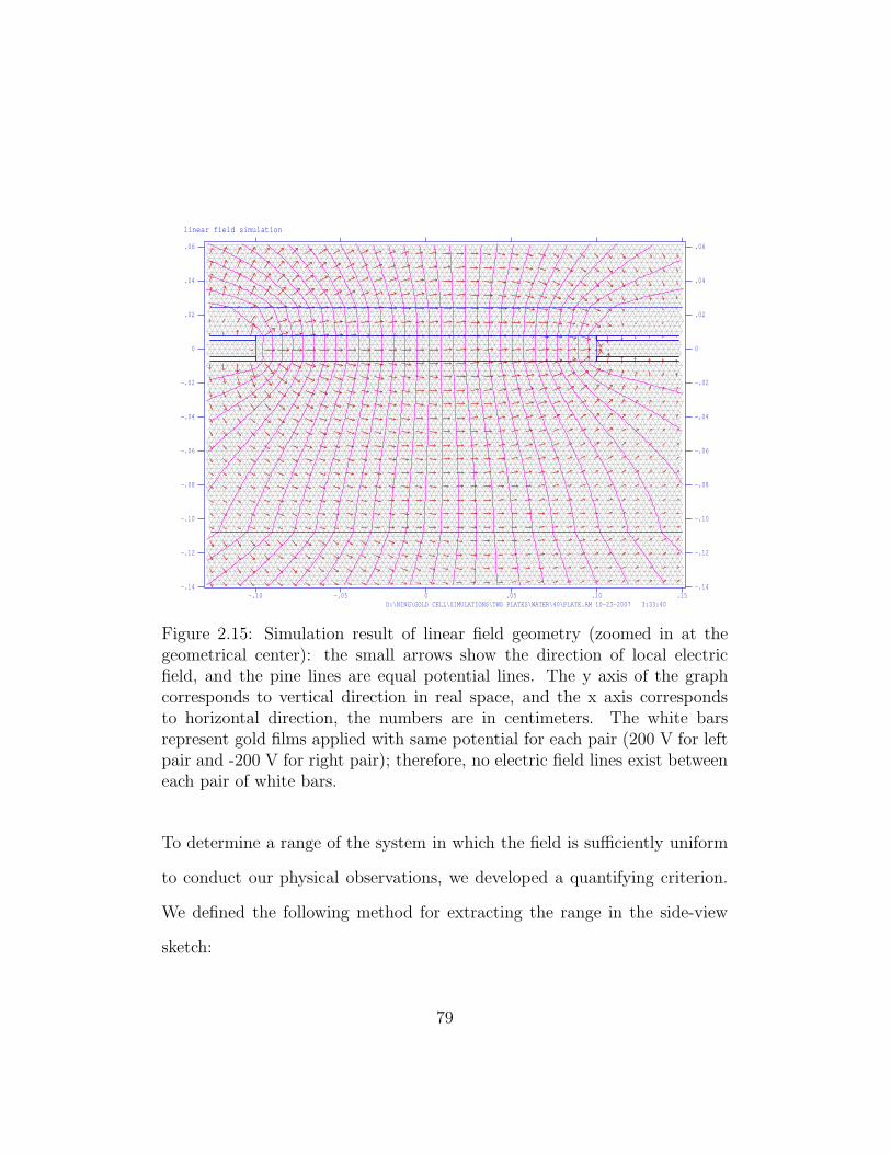
linear field simulation
D:\NING\GOLD CELL\SIMULATIONS\TWO PLATES\WATER\40\PLATE.AM 10−23−2007 3:33:40
−.14
−.12
−.10
−.08
−.06
−.04
−.02
0
.02
.04
.06
−.14
−.12
−.10
−.08
−.06
−.04
−.02
0
.02
.04
.06
−.10 −.05 0 .05 .10 .15
Figure 2.15: Simulation result of linear field geometry (zoomed in at thegeometrical center): the small arrows show the direction of local electricfield, and the pine lines are equal potential lines. The y axis of the graphcorresponds to vertical direction in real space, and the x axis correspondsto horizontal direction, the numbers are in centimeters. The white barsrepresent gold films applied with same potential for each pair (200 V for leftpair and -200 V for right pair); therefore, no electric field lines exist betweeneach pair of white bars.
To determine a range of the system in which the field is sufficiently uniform
to conduct our physical observations, we developed a quantifying criterion.
We defined the following method for extracting the range in the side-view
sketch:
79
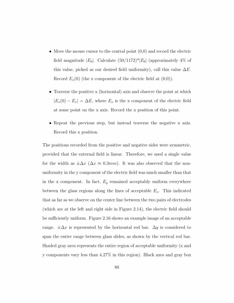
� Move the mouse cursor to the central point (0,0) and record the electric
field magnitude |E0|. Calculate (50/1172)*|E0| (approximately 4% of
this value, picked as our desired field uniformity), call this value ∆E.
Record Ex(0) (the x component of the electric field at (0,0)).� Traverse the positive x (horizontal) axis and observe the point at which
|Ex(0) − Ex| = ∆E, where Ex is the x component of the electric field
at some point on the x axis. Record the x position of this point.� Repeat the previous step, but instead traverse the negative x axis.
Record this x position.
The positions recorded from the positive and negative sides were symmetric,
provided that the external field is linear. Therefore, we used a single value
for the width as ±∆x (∆x ≈ 0.3mm). It was also observed that the non-
uniformity in the y component of the electric field was much smaller than that
in the x component. In fact, Ey remained acceptably uniform everywhere
between the glass regions along the lines of acceptable Ex. This indicated
that as far as we observe on the center line between the two pairs of electrodes
(which are at the left and right side in Figure 2.14), the electric field should
be sufficiently uniform. Figure 2.16 shows an example image of an acceptable
range. ±∆x is represented by the horizontal red bar. ∆y is considered to
span the entire range between glass slides, as shown by the vertical red bar.
Shaded gray area represents the entire region of acceptable uniformity (x and
y components vary less than 4.27% in this region). Black axes and gray box
80
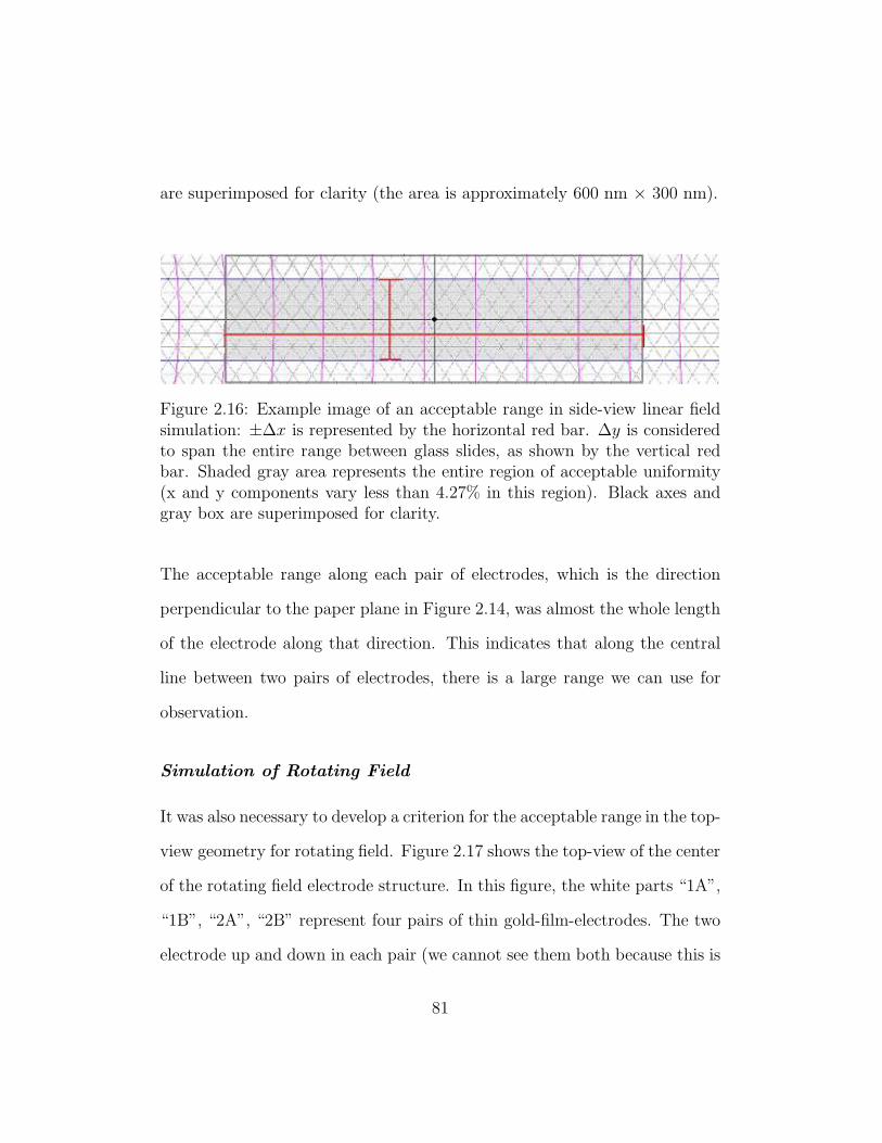
are superimposed for clarity (the area is approximately 600 nm × 300 nm).
Figure 2.16: Example image of an acceptable range in side-view linear fieldsimulation: ±∆x is represented by the horizontal red bar. ∆y is consideredto span the entire range between glass slides, as shown by the vertical redbar. Shaded gray area represents the entire region of acceptable uniformity(x and y components vary less than 4.27% in this region). Black axes andgray box are superimposed for clarity.
The acceptable range along each pair of electrodes, which is the direction
perpendicular to the paper plane in Figure 2.14, was almost the whole length
of the electrode along that direction. This indicates that along the central
line between two pairs of electrodes, there is a large range we can use for
observation.
Simulation of Rotating Field
It was also necessary to develop a criterion for the acceptable range in the top-
view geometry for rotating field. Figure 2.17 shows the top-view of the center
of the rotating field electrode structure. In this figure, the white parts “1A”,
“1B”, “2A”, “2B” represent four pairs of thin gold-film-electrodes. The two
electrode up and down in each pair (we cannot see them both because this is
81
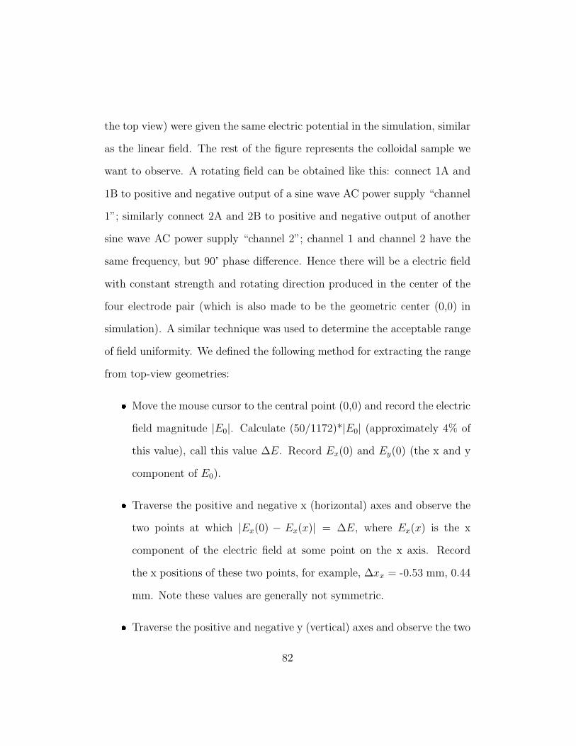
the top view) were given the same electric potential in the simulation, similar
as the linear field. The rest of the figure represents the colloidal sample we
want to observe. A rotating field can be obtained like this: connect 1A and
1B to positive and negative output of a sine wave AC power supply “channel
1”; similarly connect 2A and 2B to positive and negative output of another
sine wave AC power supply “channel 2”; channel 1 and channel 2 have the
same frequency, but 90° phase difference. Hence there will be a electric field
with constant strength and rotating direction produced in the center of the
four electrode pair (which is also made to be the geometric center (0,0) in
simulation). A similar technique was used to determine the acceptable range
of field uniformity. We defined the following method for extracting the range
from top-view geometries:� Move the mouse cursor to the central point (0,0) and record the electric
field magnitude |E0|. Calculate (50/1172)*|E0| (approximately 4% of
this value), call this value ∆E. Record Ex(0) and Ey(0) (the x and y
component of E0).� Traverse the positive and negative x (horizontal) axes and observe the
two points at which |Ex(0) − Ex(x)| = ∆E, where Ex(x) is the x
component of the electric field at some point on the x axis. Record
the x positions of these two points, for example, ∆xx = -0.53 mm, 0.44
mm. Note these values are generally not symmetric.� Traverse the positive and negative y (vertical) axes and observe the two
82
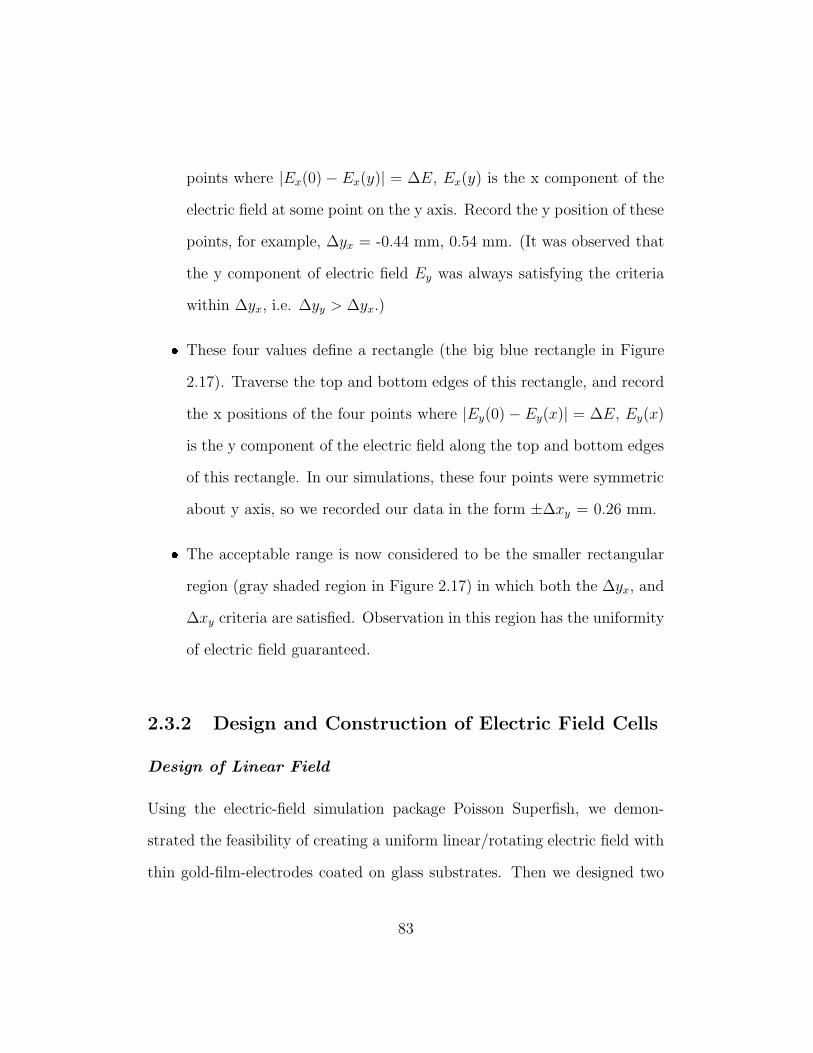
points where |Ex(0) − Ex(y)| = ∆E, Ex(y) is the x component of the
electric field at some point on the y axis. Record the y position of these
points, for example, ∆yx = -0.44 mm, 0.54 mm. (It was observed that
the y component of electric field Ey was always satisfying the criteria
within ∆yx, i.e. ∆yy > ∆yx.)� These four values define a rectangle (the big blue rectangle in Figure
2.17). Traverse the top and bottom edges of this rectangle, and record
the x positions of the four points where |Ey(0) − Ey(x)| = ∆E, Ey(x)
is the y component of the electric field along the top and bottom edges
of this rectangle. In our simulations, these four points were symmetric
about y axis, so we recorded our data in the form ±∆xy = 0.26 mm.� The acceptable range is now considered to be the smaller rectangular
region (gray shaded region in Figure 2.17) in which both the ∆yx, and
∆xy criteria are satisfied. Observation in this region has the uniformity
of electric field guaranteed.
2.3.2 Design and Construction of Electric Field Cells
Design of Linear Field
Using the electric-field simulation package Poisson Superfish, we demon-
strated the feasibility of creating a uniform linear/rotating electric field with
thin gold-film-electrodes coated on glass substrates. Then we designed two
83
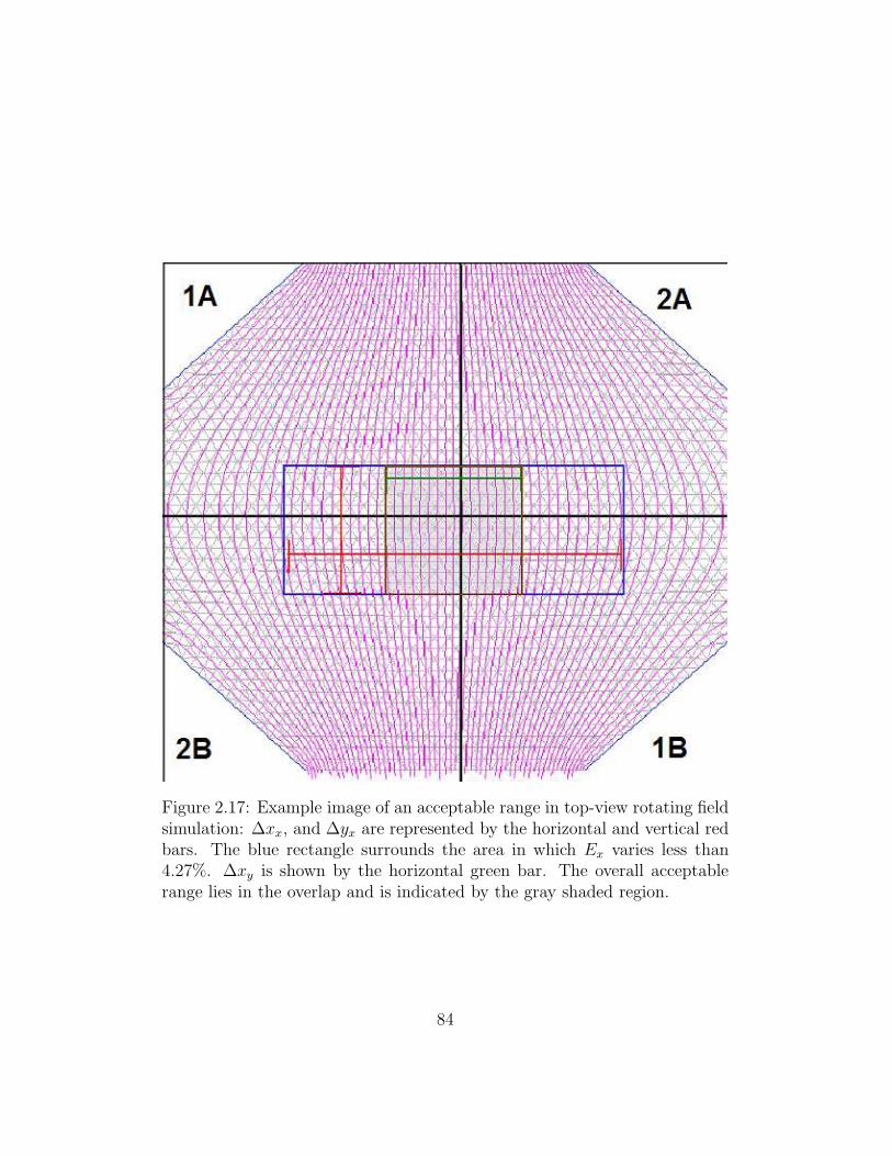
Figure 2.17: Example image of an acceptable range in top-view rotating fieldsimulation: ∆xx, and ∆yx are represented by the horizontal and vertical redbars. The blue rectangle surrounds the area in which Ex varies less than4.27%. ∆xy is shown by the horizontal green bar. The overall acceptablerange lies in the overlap and is indicated by the gray shaded region.
84
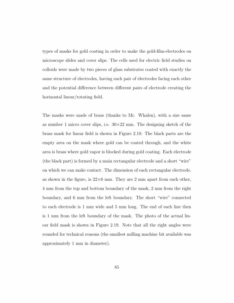
types of masks for gold coating in order to make the gold-film-electrodes on
microscope slides and cover slips. The cells used for electric field studies on
colloids were made by two pieces of glass substrates coated with exactly the
same structure of electrodes, having each pair of electrodes facing each other
and the potential difference between different pairs of electrode creating the
horizontal linear/rotating field.
The masks were made of brass (thanks to Mr. Whalen), with a size same
as number 1 micro cover slips, i.e. 30×22 mm. The designing sketch of the
brass mask for linear field is shown in Figure 2.18: The black parts are the
empty area on the mask where gold can be coated through, and the white
area is brass where gold vapor is blocked during gold coating. Each electrode
(the black part) is formed by a main rectangular electrode and a short “wire”
on which we can make contact. The dimension of each rectangular electrode,
as shown in the figure, is 22×6 mm. They are 2 mm apart from each other,
4 mm from the top and bottom boundary of the mask, 2 mm from the right
boundary, and 6 mm from the left boundary. The short “wire” connected
to each electrode is 1 mm wide and 5 mm long. The end of each line then
is 1 mm from the left boundary of the mask. The photo of the actual lin-
ear field mask is shown in Figure 2.19. Note that all the right angles were
rounded for technical reasons (the smallest milling machine bit available was
approximately 1 mm in diameter).
85
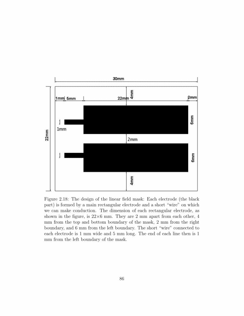
Figure 2.18: The design of the linear field mask: Each electrode (the blackpart) is formed by a main rectangular electrode and a short “wire” on whichwe can make conduction. The dimension of each rectangular electrode, asshown in the figure, is 22×6 mm. They are 2 mm apart from each other, 4mm from the top and bottom boundary of the mask, 2 mm from the rightboundary, and 6 mm from the left boundary. The short “wire” connected toeach electrode is 1 mm wide and 5 mm long. The end of each line then is 1mm from the left boundary of the mask.
86
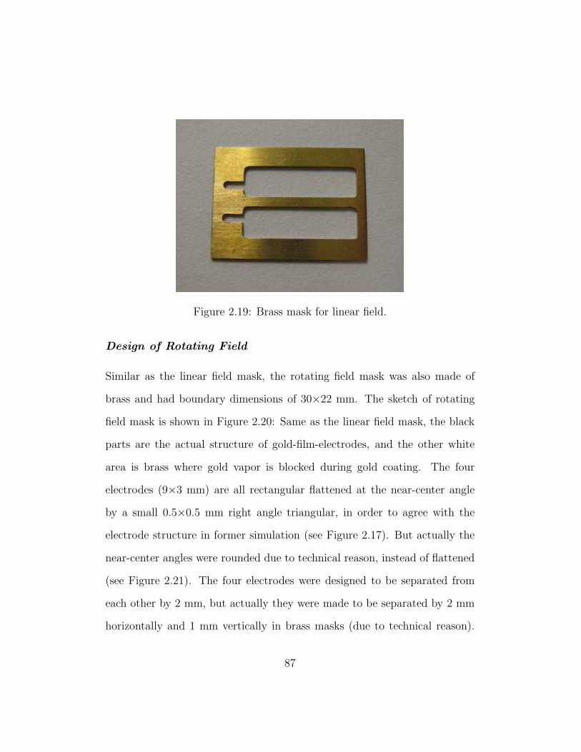
Figure 2.19: Brass mask for linear field.
Design of Rotating Field
Similar as the linear field mask, the rotating field mask was also made of
brass and had boundary dimensions of 30×22 mm. The sketch of rotating
field mask is shown in Figure 2.20: Same as the linear field mask, the black
parts are the actual structure of gold-film-electrodes, and the other white
area is brass where gold vapor is blocked during gold coating. The four
electrodes (9×3 mm) are all rectangular flattened at the near-center angle
by a small 0.5×0.5 mm right angle triangular, in order to agree with the
electrode structure in former simulation (see Figure 2.17). But actually the
near-center angles were rounded due to technical reason, instead of flattened
(see Figure 2.21). The four electrodes were designed to be separated from
each other by 2 mm, but actually they were made to be separated by 2 mm
horizontally and 1 mm vertically in brass masks (due to technical reason).
87
The electrodes are 2 mm from the right boundary of the mask, and 8 mm
from the left boundary. They were designed to be 7 mm from the top and
the bottom boundary of the mask, but were actually 7.5 mm as the verti-
cal distance between electrodes was shrunk by 1 mm. The “wires” on the
electrodes were designed to avoid overlapping of conduction joints with real
wires when making the cell. The “wires” are 1 mm wide and 2 mm away
from the left boundary of the mask. The photo of actual rotating field mask
is shown in Figure 2.21. Again all sharp corners were rounded.
Construction of Electric Field
The construction of linear and rotating electric field microscope sample cells
followed these steps:� Use the brass masks for linear and rotating field for gold coating on
micro glass slides and cover slips.
– Cut each microscope slide (VWR, 75×25 mm, 1.0 mm thick, plain)
into two identical pieces (37.5×25 mm). Prepare 8 pieces of them
and 8 micro cover slips (VWR, 30×22 mm, 0.17 mm thick) as we
have 8 linear field masks and 8 rotating field masks.
– Ultrasonicate these glass slides in soap water for approximately
30 minutes. Then clean them with tap water and distilled water.
Once there is a thin non-dewetting water layer on the glass slides,
they should be clean enough. The washed slides are then naturally
88
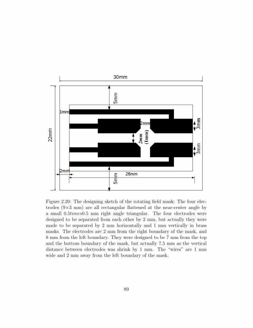
Figure 2.20: The designing sketch of the rotating field mask: The four elec-trodes (9×3 mm) are all rectangular flattened at the near-center angle bya small 0.5times0.5 mm right angle triangular. The four electrodes weredesigned to be separated from each other by 2 mm, but actually they weremade to be separated by 2 mm horizontally and 1 mm vertically in brassmasks. The electrodes are 2 mm from the right boundary of the mask, and8 mm from the left boundary. They were designed to be 7 mm from the topand the bottom boundary of the mask, but actually 7.5 mm as the verticaldistance between electrodes was shrink by 1 mm. The “wires” are 1 mmwide and 2 mm away from the left boundary of the mask.
89
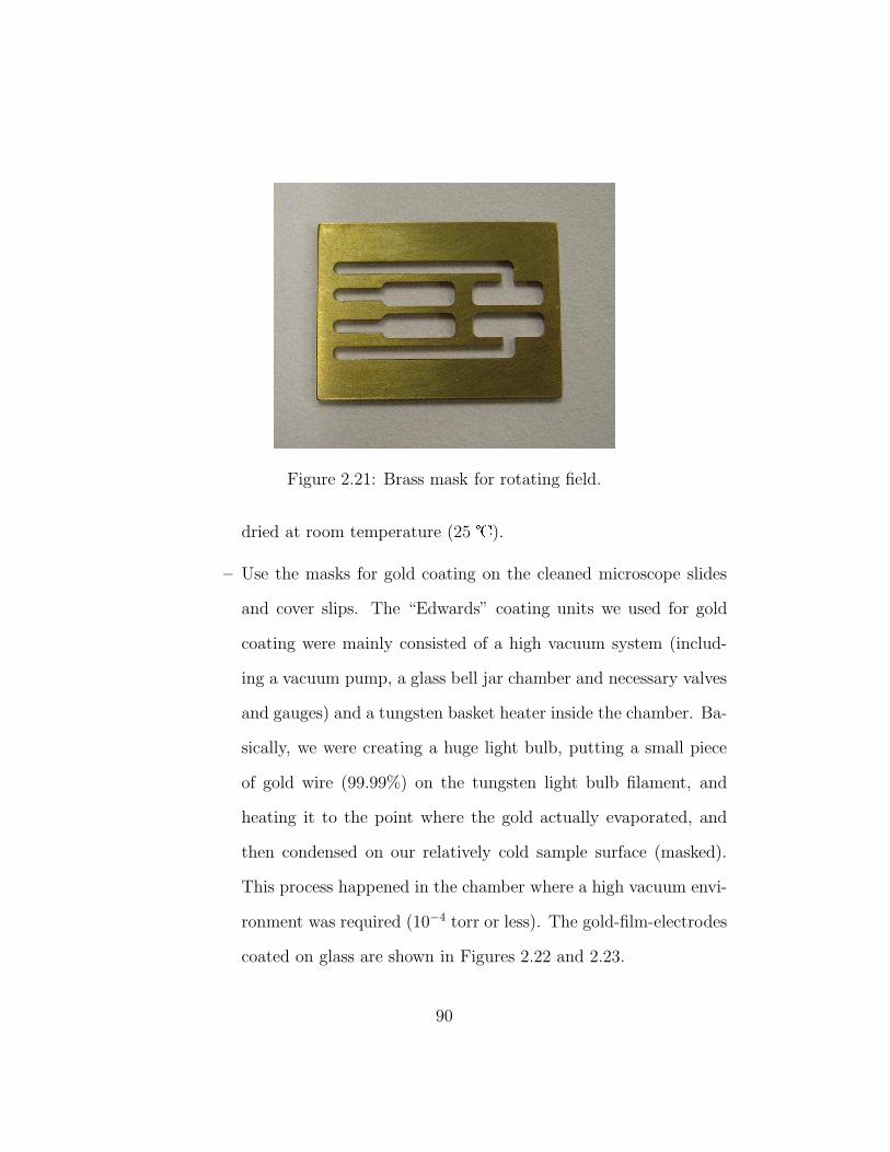
Figure 2.21: Brass mask for rotating field.
dried at room temperature (25 �).
– Use the masks for gold coating on the cleaned microscope slides
and cover slips. The “Edwards” coating units we used for gold
coating were mainly consisted of a high vacuum system (includ-
ing a vacuum pump, a glass bell jar chamber and necessary valves
and gauges) and a tungsten basket heater inside the chamber. Ba-
sically, we were creating a huge light bulb, putting a small piece
of gold wire (99.99%) on the tungsten light bulb filament, and
heating it to the point where the gold actually evaporated, and
then condensed on our relatively cold sample surface (masked).
This process happened in the chamber where a high vacuum envi-
ronment was required (10−4 torr or less). The gold-film-electrodes
coated on glass are shown in Figures 2.22 and 2.23.
90
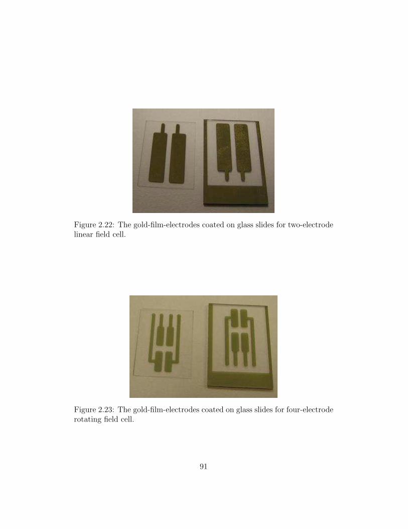
Figure 2.22: The gold-film-electrodes coated on glass slides for two-electrodelinear field cell.
Figure 2.23: The gold-film-electrodes coated on glass slides for four-electroderotating field cell.
91
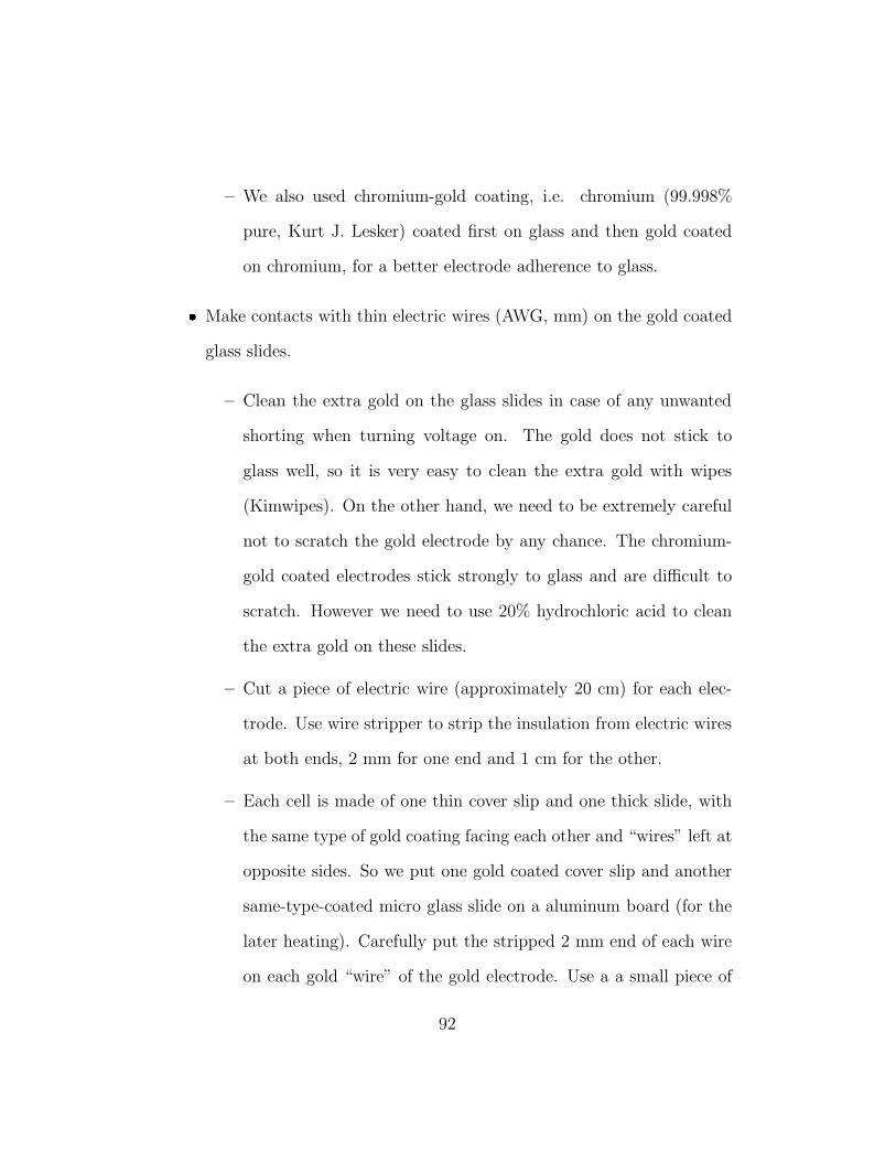
– We also used chromium-gold coating, i.e. chromium (99.998%
pure, Kurt J. Lesker) coated first on glass and then gold coated
on chromium, for a better electrode adherence to glass.� Make contacts with thin electric wires (AWG, mm) on the gold coated
glass slides.
– Clean the extra gold on the glass slides in case of any unwanted
shorting when turning voltage on. The gold does not stick to
glass well, so it is very easy to clean the extra gold with wipes
(Kimwipes). On the other hand, we need to be extremely careful
not to scratch the gold electrode by any chance. The chromium-
gold coated electrodes stick strongly to glass and are difficult to
scratch. However we need to use 20% hydrochloric acid to clean
the extra gold on these slides.
– Cut a piece of electric wire (approximately 20 cm) for each elec-
trode. Use wire stripper to strip the insulation from electric wires
at both ends, 2 mm for one end and 1 cm for the other.
– Each cell is made of one thin cover slip and one thick slide, with
the same type of gold coating facing each other and “wires” left at
opposite sides. So we put one gold coated cover slip and another
same-type-coated micro glass slide on a aluminum board (for the
later heating). Carefully put the stripped 2 mm end of each wire
on each gold “wire” of the gold electrode. Use a a small piece of
92
aluminum foil tape to stick the insulation part of the wires, for
the cover slip, onto the aluminum board. The aluminum foil tape
can endure a high temperature when we cure the conductive glue.
Similarly use this tape to stick the wires onto the microscope slide
as there is more extra space on the slide than the slip (see the
aluminum foil tape stripes in Figure 2.13, for example). We stick
the wires with the aluminum foil tape in order to hold them close
to the gold electrode “wires”, which helps keep the wires in close
contact with the gold substrate (important to minimize the joint
resistance).
– Put a small drop of conductive glue (Norland conductive adhesive
130) with a bamboo stick on each of the joints of the 2 mm stripped
section of the electric wire and the gold electrode “wire”. Put the
aluminum plate (with one cover slip, one slide and the wires on
it) into a pre-heated oven (approximately 140 �). The glue will
be precured in 5 minutes. Take out the aluminum plate to check
if the wires come off or moved, and add a little more conductive
glue if necessary. Be careful not to put too much conductive glue
that shorts the nearby electrode. The cure of the conductive glue
takes 1 hour or even more, depends on the temperature. Once the
wires and gold electrodes are checked to be conducting (using a
multimeter), we can turn the oven off.
93
� Use the microscope slide and cover slip with electric wires to make an
electric field cell.
– We use 0.075 mm thick polyethylene terephthalate film (Goodfel-
low) as the spacer between the two pieces of micro glass. Cut two
spacers (25×3 mm) from the film, wash them with 95% alcohol,
and wipe them with wipers.
– Put the spacers on sides of the glass slide where no gold were
coated on. Then put the cover slip on the slide with gold electrodes
facing inside. Carefully align the electrode pattern of the bottom
slide and the top cover slip. Put a weight or bamboo stick to
press the cover slip on the bottom slide which are separated by
the 0.075 mm spacer.
– Use bamboo stick to put little drops of No. 61 UV (ultraviolet)
glue (Norland optical adhesive 61) on side of the spacers. The glue
will go in slowly and join the top cover slip and the bottom slide
due to the capillary effect. Put this cell under a high-intensity
UV lamp (Spectroline, 365 nm wavelength) within a short dis-
tance (approximately 10 cm) for faster cure. The precure for No.
61 uv glue needs a few seconds, and the complete cure needs ap-
proximately 15 minutes.
– For a more convenient mounting of the cell on the confocal mi-
croscope, join another full length plain micro glass slide (simply
94
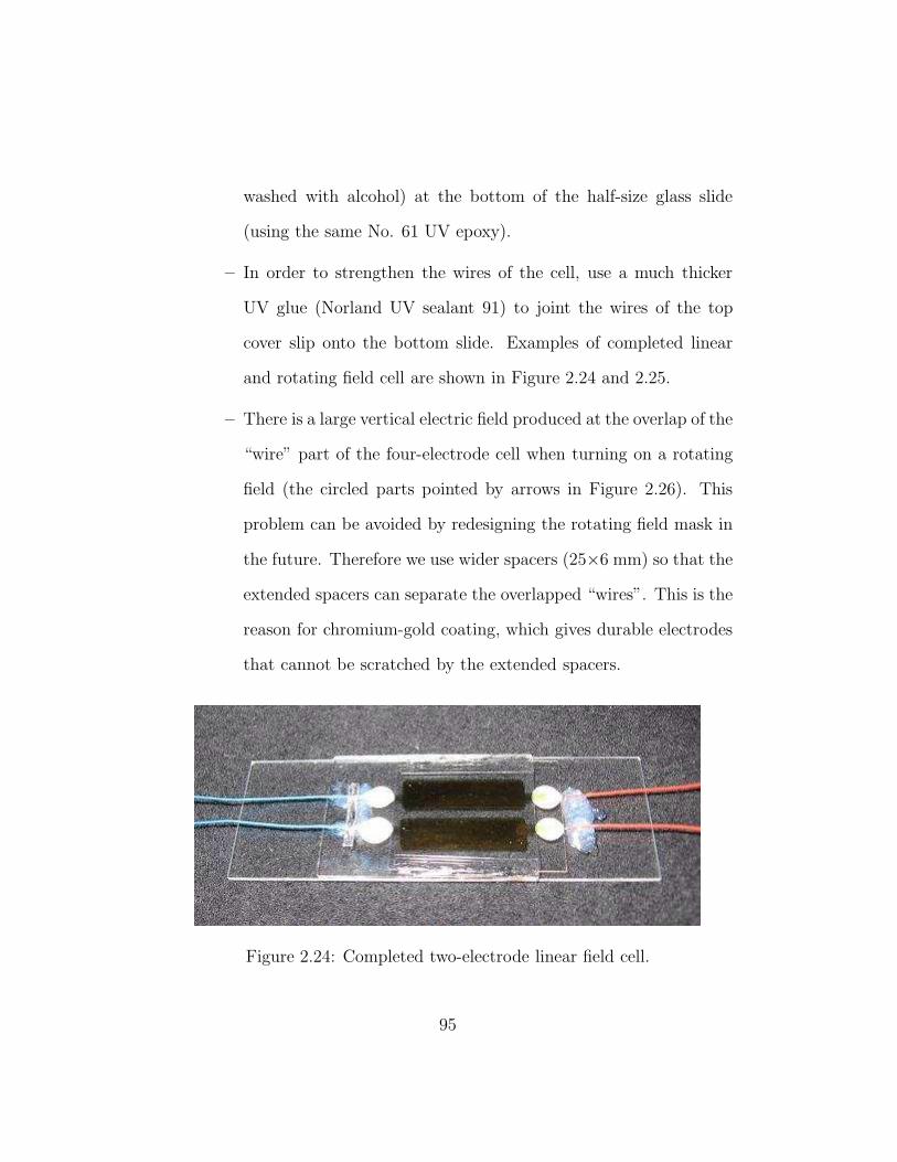
washed with alcohol) at the bottom of the half-size glass slide
(using the same No. 61 UV epoxy).
– In order to strengthen the wires of the cell, use a much thicker
UV glue (Norland UV sealant 91) to joint the wires of the top
cover slip onto the bottom slide. Examples of completed linear
and rotating field cell are shown in Figure 2.24 and 2.25.
– There is a large vertical electric field produced at the overlap of the
“wire” part of the four-electrode cell when turning on a rotating
field (the circled parts pointed by arrows in Figure 2.26). This
problem can be avoided by redesigning the rotating field mask in
the future. Therefore we use wider spacers (25×6 mm) so that the
extended spacers can separate the overlapped “wires”. This is the
reason for chromium-gold coating, which gives durable electrodes
that cannot be scratched by the extended spacers.
Figure 2.24: Completed two-electrode linear field cell.
95
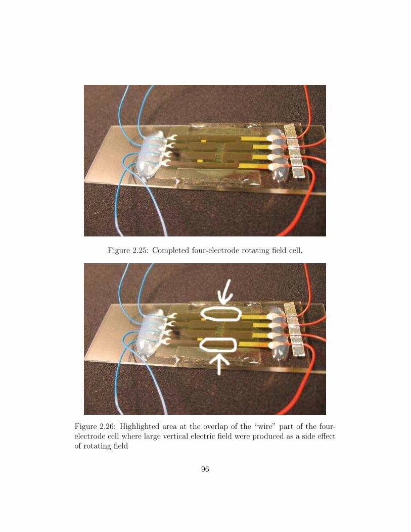
Figure 2.25: Completed four-electrode rotating field cell.
Figure 2.26: Highlighted area at the overlap of the “wire” part of the four-electrode cell where large vertical electric field were produced as a side effectof rotating field
96

Chapter 3
Experiments, Data Analysis
and Results
This chapter describes the detailed procedure for our electric field experi-
ments in sedimented colloidal suspensions, the acquisition and analysis of
quantitative data, and finally the discussion of results.
97
3.1 Experimental Procedures
This section describes general procedures for electric field experiments. Us-
ing the confocal microscope, we studied the synthesized silica colloids under
external electric fields. The confocal images were then analyzed using image-
processing programs written in the IDL programming language, the raw data
was analyzed to calculate different order parameters, and the output order
parameters were further analyzed using graphical analyzing program Igor
Pro.
3.1.1 Sample Preparation
We used synthesized silica core-shell particles (0.77µm NL9 and 1.14µm NL8,
see 2.1 for synthesis details) to prepare samples for confocal microscopy (see
2.3.2 for more details about the cell). The colloids were refractive index
matched for confocal imaging, and salt added to make the silica spheres
behave like hard spheres. The colloids were then filled in the cells made for
electric field experiments.
Refractive Index Matching
The less the mismatch between the refractive index of silica particles np and
of the surrounding fluid nf , the better the confocal image quality of fluores-
cent cores will be. This is because multiple scattering of light degrades image
quality. We did not know the exact np of our porous silica particles, but we
98
knew np ≈ 1.46. Therefore we used dimethyl sulfoxide (abbreviated DMSO,
ACP Chemicals Inc., nD = 1.479, 20 �) and distilled water (nW = 1.333, 20�) mixture to make a fluid whose nf equals np. A mixture of water:DMSO
with volume fraction ratio of 15:85 gave a relatively good result. Thus we
found that np ≈ 1.46. The original silica suspension stored in ethanol was
very milky and almost opaque. After transfer to the water:DMSO mixture,
where the same centrifuge technique was used as before, the suspension con-
tained in a 2 mL cylindrical glass vial was clear enough to easily look through.
To minimize the refractive index mismatch, we used the technique of heat-
ing or cooling the suspensions to decide whether more DMSO or water was
needed. Because the refractive index of water:DMSO mixture decreases
while the mixture is heated and increases when cooled (the temperature
dependence of refractive index for typical solvent is approximately 0.001 per
Kelvin), we can tell whether nf in the suspension is higher or lower than np
and adjust it as follows:� If the suspension (in a glass container) looks clearer when cooled with
cold tap water, or it looks more milky when heated with hot tap water,
then nf at room temperature is actually lower than np. We can add a
few drops of DMSO in the suspension to make it look clearer.� If the suspension looks clearer when heated, or it looks more milky
when cooled, then nf at room temperature is actually higher than np.
99
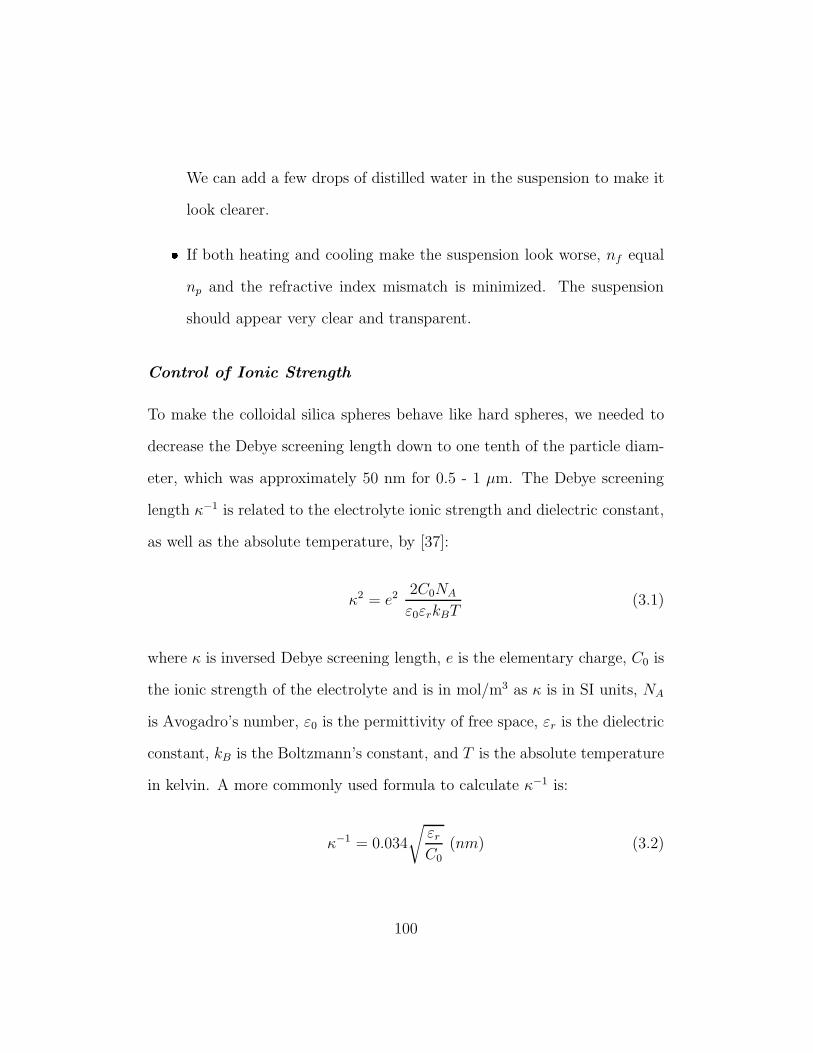
We can add a few drops of distilled water in the suspension to make it
look clearer.� If both heating and cooling make the suspension look worse, nf equal
np and the refractive index mismatch is minimized. The suspension
should appear very clear and transparent.
Control of Ionic Strength
To make the colloidal silica spheres behave like hard spheres, we needed to
decrease the Debye screening length down to one tenth of the particle diam-
eter, which was approximately 50 nm for 0.5 - 1 µm. The Debye screening
length κ−1 is related to the electrolyte ionic strength and dielectric constant,
as well as the absolute temperature, by [37]:
κ2 = e2 2C0NA
ε0εrkBT(3.1)
where κ is inversed Debye screening length, e is the elementary charge, C0 is
the ionic strength of the electrolyte and is in mol/m3 as κ is in SI units, NA
is Avogadro’s number, ε0 is the permittivity of free space, εr is the dielectric
constant, kB is the Boltzmann’s constant, and T is the absolute temperature
in kelvin. A more commonly used formula to calculate κ−1 is:
κ−1 = 0.034
√
εr
C0
(nm) (3.2)
100
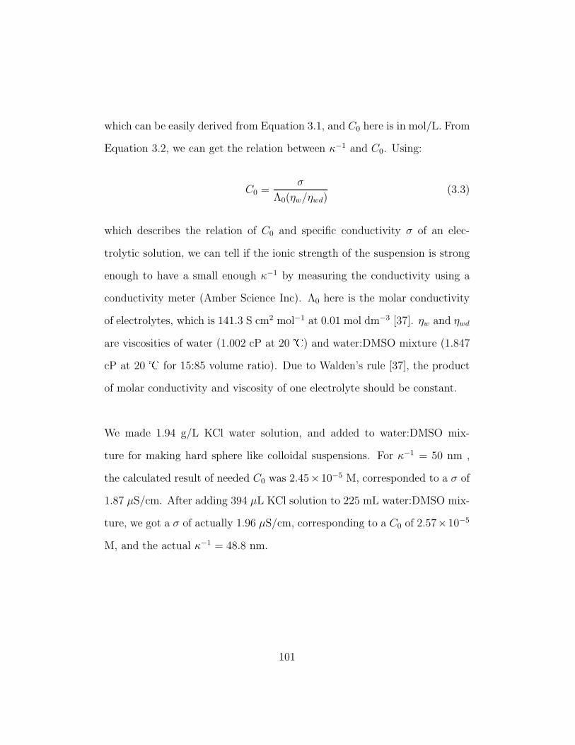
which can be easily derived from Equation 3.1, and C0 here is in mol/L. From
Equation 3.2, we can get the relation between κ−1 and C0. Using:
C0 =σ
Λ0(ηw/ηwd)(3.3)
which describes the relation of C0 and specific conductivity σ of an elec-
trolytic solution, we can tell if the ionic strength of the suspension is strong
enough to have a small enough κ−1 by measuring the conductivity using a
conductivity meter (Amber Science Inc). Λ0 here is the molar conductivity
of electrolytes, which is 141.3 S cm2 mol−1 at 0.01 mol dm−3 [37]. ηw and ηwd
are viscosities of water (1.002 cP at 20 �) and water:DMSO mixture (1.847
cP at 20 � for 15:85 volume ratio). Due to Walden’s rule [37], the product
of molar conductivity and viscosity of one electrolyte should be constant.
We made 1.94 g/L KCl water solution, and added to water:DMSO mix-
ture for making hard sphere like colloidal suspensions. For κ−1 = 50 nm ,
the calculated result of needed C0 was 2.45×10⁻⁵ M, corresponded to a σ of
1.87 µS/cm. After adding 394 µL KCl solution to 225 mL water:DMSO mix-
ture, we got a σ of actually 1.96 µS/cm, corresponding to a C0 of 2.57×10⁻⁵
M, and the actual κ−1 = 48.8 nm.
101
Control of Sample Concentration and Sample Filling
The volume fraction of our colloidal samples was measured using the same
oven-drying method as described in last chapter, assuming the density of
porous silica sphere was 2 g/mL. Volume fractions for the samples we used
were as follows:� 3.1% 0.77 µm core-shell silica colloids (NL9B1), salted (i.e. KCl added),
used for Experiment S1 (described in next section).� 3.8% 1.14 µm core-shell silica colloids (NL8B), salted, used for Exper-
iment L1.� 3.1% 0.77 µm core-shell silica colloids (NL9B2), unsalted (i.e. water
and DMSO only), used for Experiment S2.
After making the samples, we stored each of them separately in 2 mL black
cap glass vials. Before experiments, we stirred the sample using a vortexer
(Vortex Genie 2, Scientific Industries) and ultrasonicated it for approximately
30 minutes to make the volume fraction uniform. Then a disposable Pasteur
pipette (534
inches, Fisherbrand) was used to take the sample, by dipping the
tip of the pipette in the sample. The capillary action drove the sample into
the pipette, although only a small amount. The sample was then transferred
to the electric field cell we made by touching the pipette tip to the edge of
the cell, again due to the capillary action. This was repeated a few times
102
until the cell was fully filled. We tried to avoid creating any air bubbles while
filling the cell, which otherwise can affect the uniformity of the electric field.
3.1.2 Experimental Setup
Here we introduce the experimental setup, including setup for electric field
instruments and configurations for our confocal microscope.
Electric Field Setup
The instruments we used to generate electric fields were a dual-channel func-
tion generator (0-25 MHz, Tektronix, AFG3022) and two wide-band ampli-
fiers (DC/0-1 MHz, Krohn-Hite, 7602M), and a two-channel digital storage
oscilloscope (0-10 MHz, Tektronix, TDS1002) for monitoring AC voltages.
For the two-electrode linear field cell (described in 2.3.2), only one channel
of the function generator and one amplifier was used. One pair of verti-
cally overlapped electrodes was connected to the positive output via wires,
the other pair was grounded. We used the function generator to generate
a 1 MHz, sinusoidally alternating signal, and used the amplifier to generate
different amplitudes of potentials. The signal amplitude from the function
generator was 1 V (peak-to-peak potential, same for follows). Both the am-
plitudes generated from generator and the amplifier can be gradually varied
to change the output. The amplitude control in the generator was especially
useful as the amplitude control in the amplifier gave too large fluctuation in
103
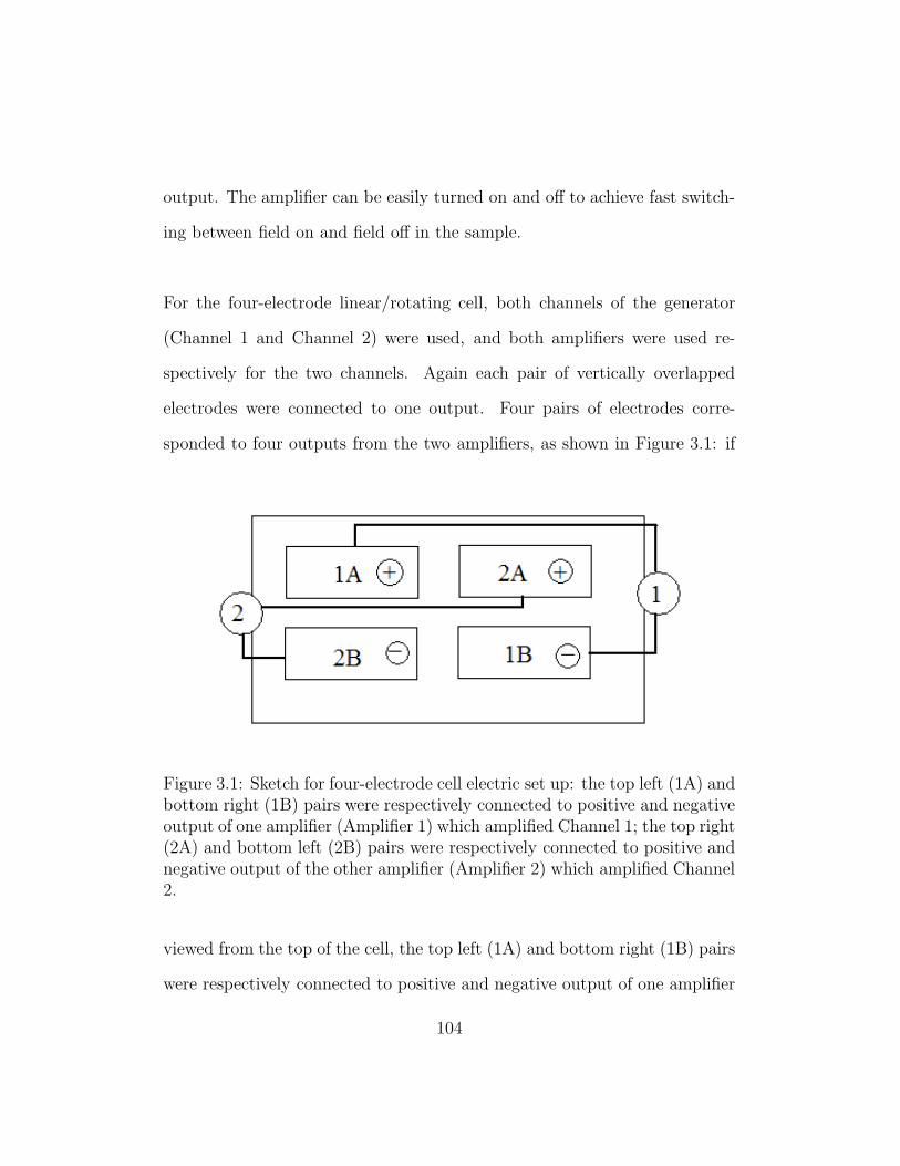
output. The amplifier can be easily turned on and off to achieve fast switch-
ing between field on and field off in the sample.
For the four-electrode linear/rotating cell, both channels of the generator
(Channel 1 and Channel 2) were used, and both amplifiers were used re-
spectively for the two channels. Again each pair of vertically overlapped
electrodes were connected to one output. Four pairs of electrodes corre-
sponded to four outputs from the two amplifiers, as shown in Figure 3.1: if
Figure 3.1: Sketch for four-electrode cell electric set up: the top left (1A) andbottom right (1B) pairs were respectively connected to positive and negativeoutput of one amplifier (Amplifier 1) which amplified Channel 1; the top right(2A) and bottom left (2B) pairs were respectively connected to positive andnegative output of the other amplifier (Amplifier 2) which amplified Channel2.
viewed from the top of the cell, the top left (1A) and bottom right (1B) pairs
were respectively connected to positive and negative output of one amplifier
104
(Amplifier 1) which amplified Channel 1; the top right (2A) and bottom left
(2B) pairs were respectively connected to positive and negative output of the
other amplifier (Amplifier 2) which amplified Channel 2. Note that Channel
1/2 and Amplifier 1/2 were arbitrarily chosen, and should not affect the re-
sult if 1 and 2 were completely switched. We used negative output instead
of ground in order to achieve symmetric rotating field. The detector of the
oscilloscope, however, can only measure the potential to ground because one
of the two connections on the detector was designed to be grounded through
the oscilloscope. Therefore we had to use the other connection of the detector
connecting only the positive output of the amplifier, knowing the actual po-
tential was twice as high as shown on the oscilloscope. We again used 1 MHz
sinusoidally alternating signal, but for rotating field there was a 90° phase
shift from channel 2 to channel 1, while for linear field there was no phase
difference between the two channels. The amplitudes of potentials from the
two amplifiers were always kept the same for either rotating field or linear
field, in order to have a spatially uniform field near the center of the four
electrodes.
Microscope Configuration
The confocal microscope we used consists of a Nikon fluorescent inverted
microscope, a VisiTech confocal scanning unit equipped with a 491 nm laser.
The configurations in the confocal microscope and the confocal controlling
software “VoxCell” were as follows:
105
� 100×/1.40 Oil objective� 50 µm aperture� 700 × 700 pixels� 29 frames per second (fps) scan speed� 8 bit data (for output images)� 1× amplification
To optimize the quality of the confocal images, one needs to adjust laser
power and photomultiplier tubes (PMT) gain using the VoxCell software for
the 491 nm laser we used.
3.1.3 Experiment Procedure
The operational procedure of the three electric field experiments is described
here, including linear field experiment for NL9B1 0.77 µm silica particles
(Experiment S1, as it is the first experiment using relatively small size silica
colloids) and NL8B 1.14 µm particles (Experiment L1, as it is the first ex-
periment using relatively large size silica colloids), and rotating/linear field
experiment for NL9B2 0.77 µm particles (Experiment S2, as it is the second
experiment using relatively small size silica colloids).
106
Experiment S1
This experiment, using 0.77 µm diameter silica colloids (NL9B1, salted,
κa = 7.9 where a is particle radius) under linear fields created by a two-
electrode cell (2 mm between the two electrodes, see 2.3.2), was completed
in a procedure as follows:� Sedimentation profile.
– A confocal z-scan was carried out for the full range of sedimented
silica particles. Analyze the data with IDL procedure nl 3dhisto-
.pro and obtain a profile of particle number distribution along
sedimenting direction, i.e. z direction.
– Load the IDL data to Igor Pro, calculate the volume fraction (φ)
distribution along z steps (Z, integers start from 0). The step-
size along z of the confocal image acquisition (stored in the vari-
able “stepsize”) was chosen to be roughly half of the particle
diameter (i.e. 0.4 µm). Data from a number (stored in the vari-
able “binsize”) of consecutive steps were binned together. Typ-
ically, the variable binsize and stepsize were chosen such that
binsize × stepsize ≈ particle diameter (see Figure 3.2). In or-
der to calculate local volume fraction in one bin we can simply
multiply the particle numbers found by a constant (Cφ):
Cφ =Vp
Vbin
(3.4)
107
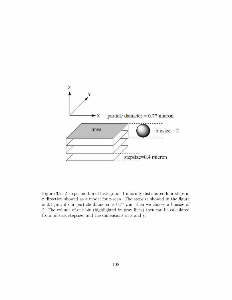
Figure 3.2: Z steps and bin of histogram: Uniformly distributed four steps inz direction showed as a model for z-scan. The stepsize showed in the figureis 0.4 µm; if our particle diameter is 0.77 µm, then we choose a binsize of2. The volume of one bin (highlighted by gray lines) then can be calculatedfrom binsize, stepsize, and the dimensions in x and y.
108
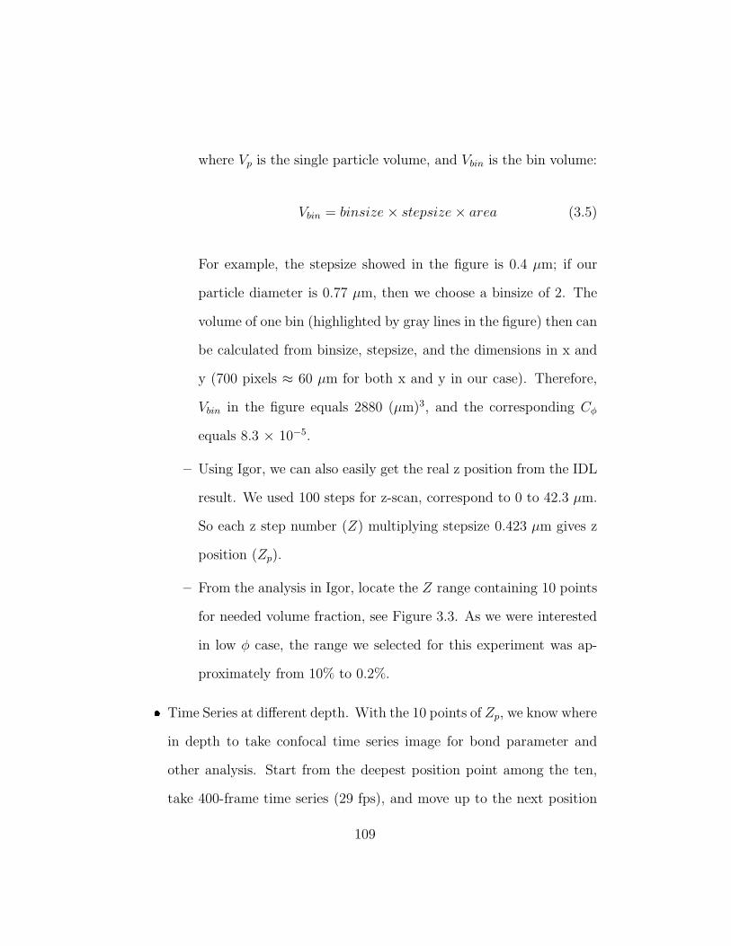
where Vp is the single particle volume, and Vbin is the bin volume:
Vbin = binsize × stepsize × area (3.5)
For example, the stepsize showed in the figure is 0.4 µm; if our
particle diameter is 0.77 µm, then we choose a binsize of 2. The
volume of one bin (highlighted by gray lines in the figure) then can
be calculated from binsize, stepsize, and the dimensions in x and
y (700 pixels ≈ 60 µm for both x and y in our case). Therefore,
Vbin in the figure equals 2880 (µm)3, and the corresponding Cφ
equals 8.3 × 10⁻⁵.
– Using Igor, we can also easily get the real z position from the IDL
result. We used 100 steps for z-scan, correspond to 0 to 42.3 µm.
So each z step number (Z) multiplying stepsize 0.423 µm gives z
position (Zp).
– From the analysis in Igor, locate the Z range containing 10 points
for needed volume fraction, see Figure 3.3. As we were interested
in low φ case, the range we selected for this experiment was ap-
proximately from 10% to 0.2%.� Time Series at different depth. With the 10 points of Zp, we know where
in depth to take confocal time series image for bond parameter and
other analysis. Start from the deepest position point among the ten,
take 400-frame time series (29 fps), and move up to the next position
109
0.18
0.16
0.14
0.12
0.10
0.08
0.06
0.04
0.02
0.00
Vol
ume
frac
tion
1009080706050403020100Z step
Range Interested
Figure 3.3: Example of sedimentation profile. The “Range Interested” in thefigure shows the general Z range of interest for confocal time series experi-ments.
to take another 400-frame time series.� Vary fields. We started from no field, and repeated the whole procedure
at different values of linear field. We took 11 values between 0 V and
300 V, and the values were almost equally distributed (in volt): 0, 50,
100, 120, 150, 180, 200, 220, 250, 280, 300. Note the corresponding
fields here were just these potentials divided by 2 mm.� Analyze these time series using IDL procedures nl bondensity.pro, nl -
bondtheta.pro and nl ericgr2d.pro, etc to get bond order parameters
and pair correlation functions.� Load all these data to Igor Pro for analysis.
110
Experiment L1
This experiment, using 1.14 µm diameter salted silica colloids (NL8B, κa =
11.7 where a is particle radius) under linear fields created by a two-electrode
cell (2 mm between), was completed in a procedure similar to Experiment S1.
We used the moving average method for z profile as mentioned in 2.2.2,
due to the relatively large particle diameter. We did 100 z steps through 30
µm, therefore the stepsize is 0.3 µm and binsize is 4, leading to a 1.2 µm
thick bin slide. However, we shifted every 2 frames (i.e. 0.6 µm) in z-stack
to get more finely-spaced data.
We took 11 equally (every 20 V) separated values from 0 to 200 V as the
potentials across the 2 mm electrode gap, corresponding to 11 fields from 0
to 1000 V/cm.
Experiment S2
This experiment, using 0.77 µm unsalted silica colloids (NL9B2) under lin-
ear/rotating fields created by a four-electrode cell (see 2.3.2 for details), was
again completed in a similar procedure.
The reason we used unsalted colloids for this experiments is that the ver-
tical field created at the overlaps of the electrode “wires”, as we mentioned
in 2.3.2. When a rotating field was applied on the four-electrode cell, a poten-
111
tial difference between the top and bottom electrodes created a high vertical
electric field at the overlap parts of the “wires”. Sample with higher ionic
strength would produce more heat, dangerous for the 100× objective which
was closely touching the cell. Therefore, we switched to a unsalted 0.77 µm
sample with same concentration.
We took 11 values from 0 V to 240 V, for both linear and rotating fields.
From the simulation results we had an estimate for the actual fields at the
center of the four electrodes where we observed the colloids through the mi-
croscope. These fields were not the same for the linear field and rotating
field, and different from the two-electrode case. This was simply due to dif-
ferent electrode geometries. For example, a 200 V potential corresponded
to a 1000 V/cm linear field in the two-electrode cell. But for four-electrode
cell, the linear field produced by 200 V was 820 V/cm, and the rotating field
produced by the same potential was 580 V/cm (1/√
2 of linear field).
When doing the experiment, we switched between linear and rotating field
(i.e. switched the phase difference between Channel 1 and Channel 2 between
0°and 90°) at all the ten places in depth and also at all 11 potential values, in
order to obtain the sedimentation profile and time series images for these two
types of field. To assure the colloids were at equilibrium state, the switching
of the field type was not faster than once per minute. The advantage of this
method was having the linear/rotating phase transition observed at the same
112

place in the plane. Even if there was any vertical shift (there actually was
a little as we will show later), we would not lose any information in local
volume fraction, since we had the sedimentation profile separately taken for
each type of field.
3.2 Data Acquisition, Analysis and Results
In this section, we will present the detailed methods of data acquisition and
analysis, as mentioned in 3.1.3 at the last step of the experiment procedure.
3.2.1 Data Acquisition
From all the confocal images taken in each experiment, we used IDL to
calculate bond parameters. We also used Igor Pro to help determine the
proper parameters of IDL procedures described in 2.2.
Data Naming Convention
In one experiment, for each value of potential we had ten time series with dif-
ferent local volume fractions. Normally a 400-frame time series was exported
with a name containing information of both potential and volume fraction.
Since the sedimented silica colloids showed a decreasing local volume fraction
upon decreasing depth and we started from the lowest point, normally the
first time series was the most dense one. For example, the first time series
taken at 20 V, which had the highest local volume fraction, would be named
113
as “020v ts1”; and the last one with the lowest volume fraction would be
“020v ts10”.
Systematic Method For Setting Brightness Thresholds
Identifying features via image processing is an imperfect science, with a del-
icate balance between cutoffs which allow no spurious particles and cutoffs
that do not miss any real particles. When acquiring z-stacks, it is possible
by correlating particles in adjacent frames to obtain a very reliable measure
of particle. When obtaining time series, the results were more sensitive to
the value of the brightness parameter (i.e. the brightness threshold) used.
We devised (and describe here) a self-consistent procedure to treat all time
series images in the same way.
The brightness threshold turned out to be an important parameter in the IDL
procedures (i.e. “nl bondensity.pro”, “nl bondtheta.pro” and “nl ericgr2d-
.pro”) for calculating the colloidal order parameter, because the number of
identified particles within an image was sensitive to the brightness used. Too
low a brightness threshold allows the identification of noise as spurious parti-
cles. Increasing the brightness threshold progressively decreased the number
of real particles that are found. To minimize the instability and subjectivity
of human judgment, we plotted the calculated bond densities of the time se-
ries image at maximum volume fraction (ts1) as a function of the brightness
threshold used. An example from Experiment S1 was shown in Figure 3.4.
114
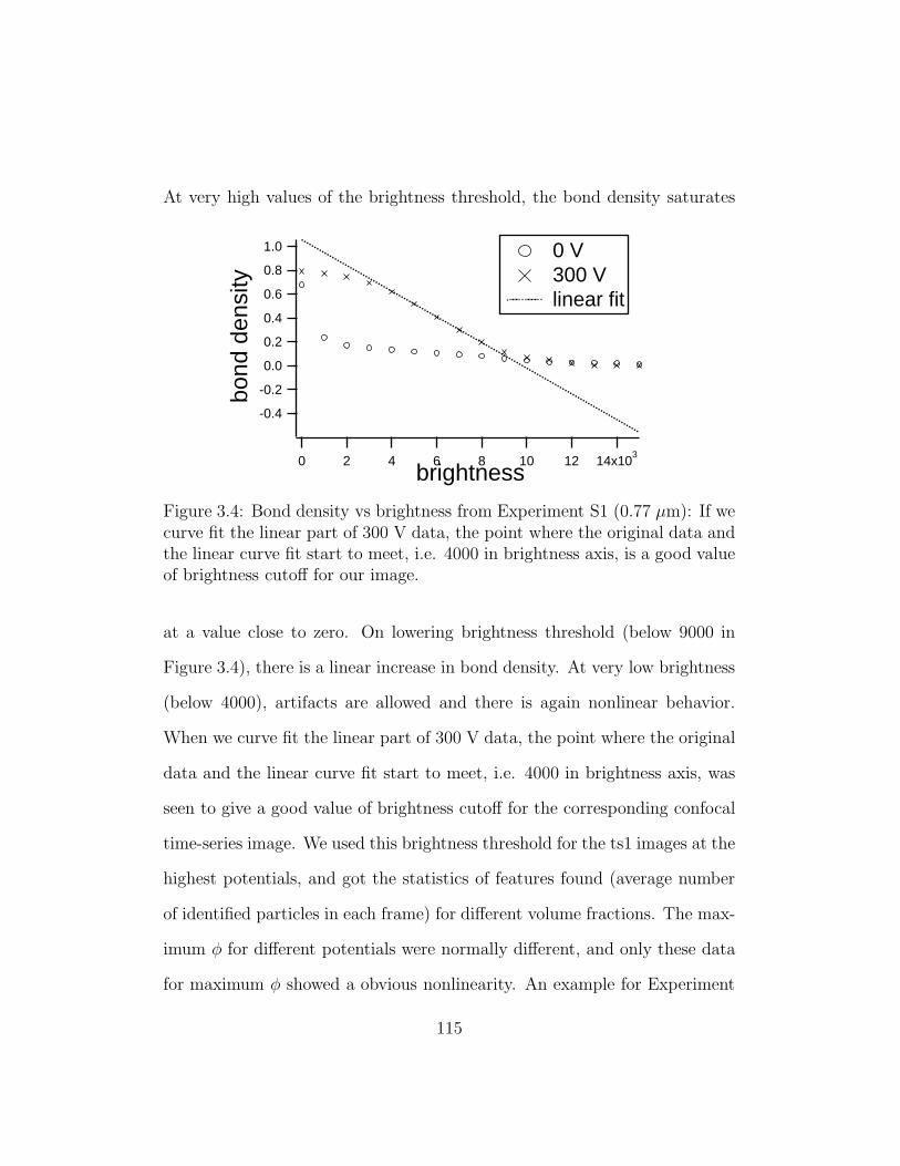
At very high values of the brightness threshold, the bond density saturates
1.0
0.8
0.6
0.4
0.2
0.0
-0.2
-0.4
bond
den
sity
14x103
121086420brightness
0 V 300 V linear fit
Figure 3.4: Bond density vs brightness from Experiment S1 (0.77 µm): If wecurve fit the linear part of 300 V data, the point where the original data andthe linear curve fit start to meet, i.e. 4000 in brightness axis, is a good valueof brightness cutoff for our image.
at a value close to zero. On lowering brightness threshold (below 9000 in
Figure 3.4), there is a linear increase in bond density. At very low brightness
(below 4000), artifacts are allowed and there is again nonlinear behavior.
When we curve fit the linear part of 300 V data, the point where the original
data and the linear curve fit start to meet, i.e. 4000 in brightness axis, was
seen to give a good value of brightness cutoff for the corresponding confocal
time-series image. We used this brightness threshold for the ts1 images at the
highest potentials, and got the statistics of features found (average number
of identified particles in each frame) for different volume fractions. The max-
imum φ for different potentials were normally different, and only these data
for maximum φ showed a obvious nonlinearity. An example for Experiment
115
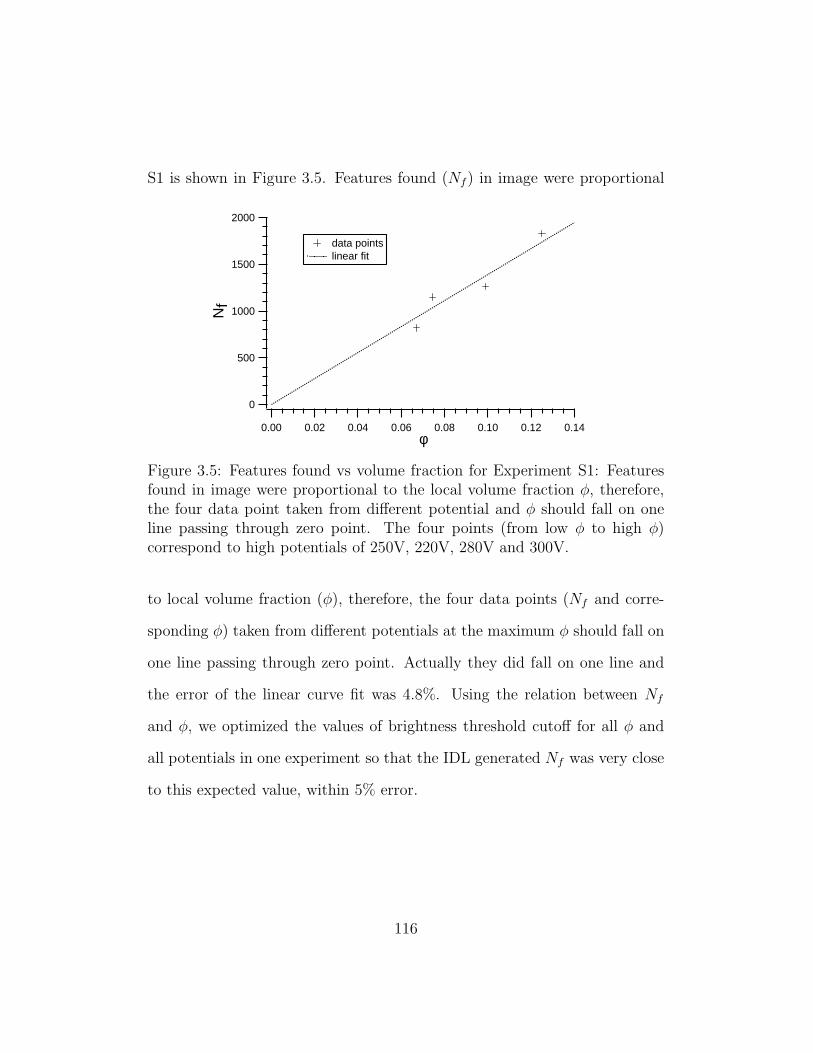
S1 is shown in Figure 3.5. Features found (Nf) in image were proportional
2000
1500
1000
500
0
Nf
0.140.120.100.080.060.040.020.00φ
data points linear fit
Figure 3.5: Features found vs volume fraction for Experiment S1: Featuresfound in image were proportional to the local volume fraction φ, therefore,the four data point taken from different potential and φ should fall on oneline passing through zero point. The four points (from low φ to high φ)correspond to high potentials of 250V, 220V, 280V and 300V.
to local volume fraction (φ), therefore, the four data points (Nf and corre-
sponding φ) taken from different potentials at the maximum φ should fall on
one line passing through zero point. Actually they did fall on one line and
the error of the linear curve fit was 4.8%. Using the relation between Nf
and φ, we optimized the values of brightness threshold cutoff for all φ and
all potentials in one experiment so that the IDL generated Nf was very close
to this expected value, within 5% error.
116
Separation Threshold
The diameter and separation setting in IDL procedures were determined
using the line tool in ImageJ and the actual diameters of particles. For
example, a diameter of 9 pixels and a separation of 9 pixels were used for
0.77 µm particle, 11 pixels and 13 pixels for 1.14 µm particle. The bond
length used for IDL procedures were 11 pixels (i.e. 0.95 µm) for 0.77 µm
particle, and 16 pixels (1.37 µm) for 1.14 µm particle.
Dipolar Energy
We calculated the bond density B and the angular order parameter 〈cos2 θ〉
from the particle coordinates obtained from our confocal images. We then
used simple do-loop procedures (these “macros” were written in the graphical
analysis program, Igor Pro) to analyze all these data (Igor Pro procedures
used are included in appendix B). The procedures consisted of operations on
data for each value of electric fields with loops running through the analysis
for data at all values of fields (see next subsection for detailed results).
This was a convenient way to study the physical parameters of interest
of colloidal suspensions upon increasing electric field energy 〈E2〉, where
〈E2〉 = 〈 ~E · ~E〉, and ~E is the center rms (root mean square) electric field. In
all the linear field experiments the 〈E2〉 is simply half of the square of E0 for
Experiment S1 and Experiment L1 (where E0 is the center field amplitude
117
of field), because:
〈 ~E · ~E〉 =E2
0
2π
∫ 2π
0
cos2 θ dθ = E20/2 . (3.6)
Although the center field amplitude E0 was different for rotating field and
linear field in Experiment S2, as we mentioned in 3.1.3, 〈E2〉 was the same
for them because:
〈 ~Erot · ~Erot〉 = (Erot0 )2 cos2 θ + (Erot
0 )2 sin2 θ = (Erot0 )2 . (3.7)
Given the same potential, the center linear field amplitude Elin0 is
√2 times
larger than the center rotating field amplitude Erot0 as:
(Erot0 )2 =
(
Elin0√2
)2
= (Elin0 )2/2 = 〈 ~Elin · ~Elin〉 . (3.8)
So we have
〈(Erot)2〉 = 〈(Elin)2〉 = E20/2 , (3.9)
where
E0 =Vpk
2d. (3.10)
Vpk here is the peak-to-peak potential, d is the distance between two lin-
ear electrodes. As we have seen in Equation 1.4, lambda parameter Λ is
a good parameter representing dipolar energy, which is proportional to the
field strength as shown in Equation 1.3. We plotted E0 vs Λ for both sizes
118
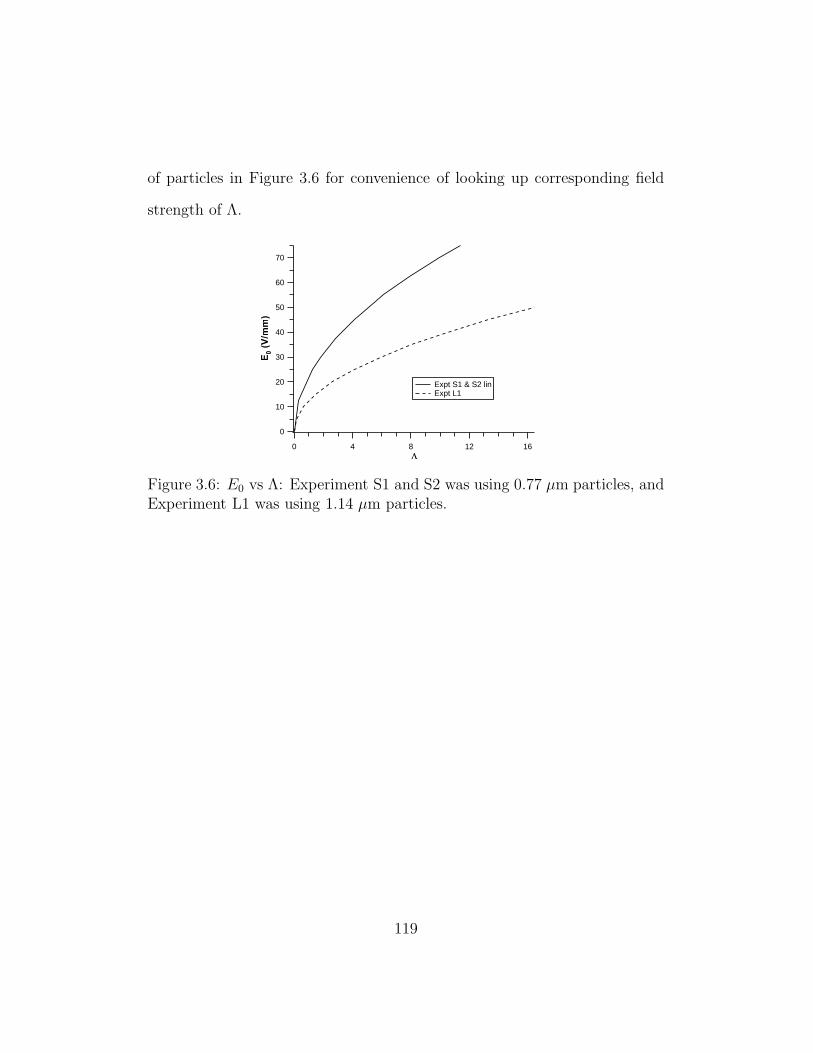
of particles in Figure 3.6 for convenience of looking up corresponding field
strength of Λ.
70
60
50
40
30
20
10
0
E0 (
V/m
m)
1612840L
Expt S1 & S2 lin Expt L1
Figure 3.6: E0 vs Λ: Experiment S1 and S2 was using 0.77 µm particles, andExperiment L1 was using 1.14 µm particles.
119
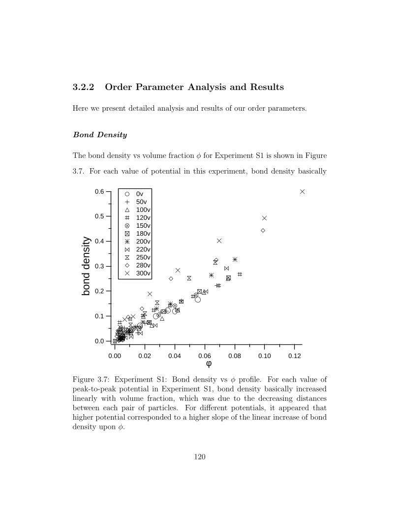
3.2.2 Order Parameter Analysis and Results
Here we present detailed analysis and results of our order parameters.
Bond Density
The bond density vs volume fraction φ for Experiment S1 is shown in Figure
3.7. For each value of potential in this experiment, bond density basically
0.6
0.5
0.4
0.3
0.2
0.1
0.0
bond
den
sity
0.120.100.080.060.040.020.00φ
0v 50v 100v 120v 150v 180v 200v 220v 250v 280v 300v
Figure 3.7: Experiment S1: Bond density vs φ profile. For each value ofpeak-to-peak potential in Experiment S1, bond density basically increasedlinearly with volume fraction, which was due to the decreasing distancesbetween each pair of particles. For different potentials, it appeared thathigher potential corresponded to a higher slope of the linear increase of bonddensity upon φ.
120
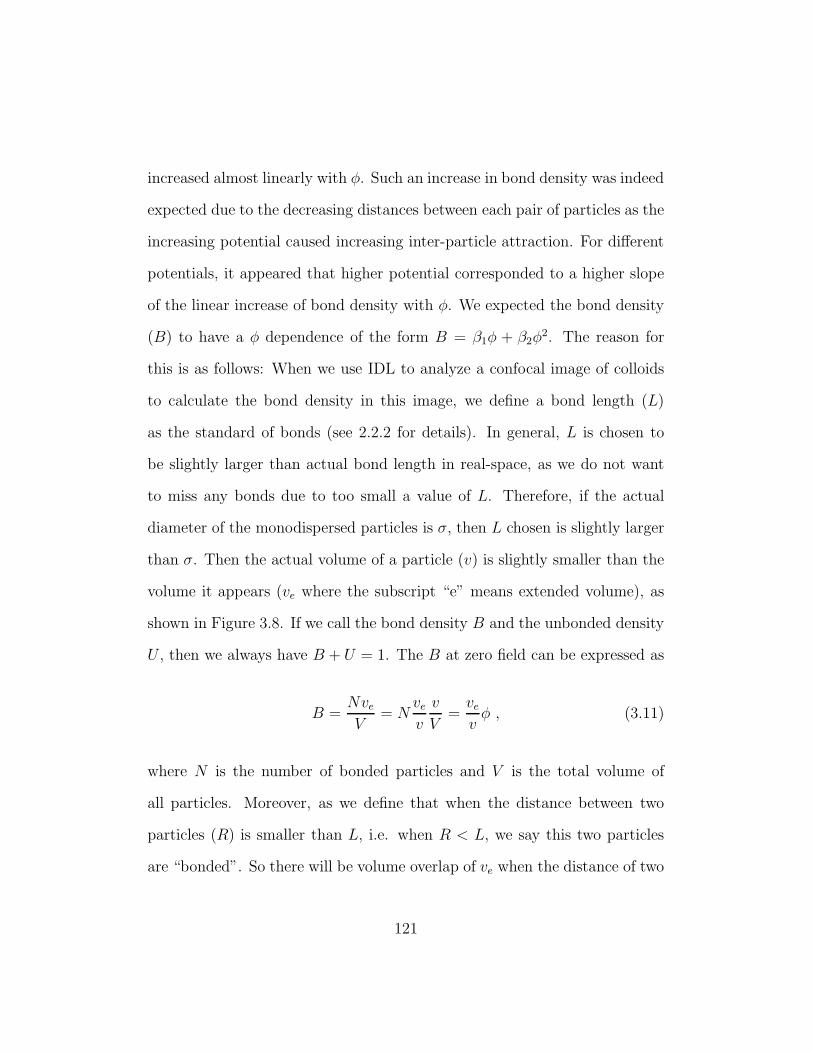
increased almost linearly with φ. Such an increase in bond density was indeed
expected due to the decreasing distances between each pair of particles as the
increasing potential caused increasing inter-particle attraction. For different
potentials, it appeared that higher potential corresponded to a higher slope
of the linear increase of bond density with φ. We expected the bond density
(B) to have a φ dependence of the form B = β1φ + β2φ2. The reason for
this is as follows: When we use IDL to analyze a confocal image of colloids
to calculate the bond density in this image, we define a bond length (L)
as the standard of bonds (see 2.2.2 for details). In general, L is chosen to
be slightly larger than actual bond length in real-space, as we do not want
to miss any bonds due to too small a value of L. Therefore, if the actual
diameter of the monodispersed particles is σ, then L chosen is slightly larger
than σ. Then the actual volume of a particle (v) is slightly smaller than the
volume it appears (ve where the subscript “e” means extended volume), as
shown in Figure 3.8. If we call the bond density B and the unbonded density
U , then we always have B + U = 1. The B at zero field can be expressed as
B =Nve
V= N
ve
v
v
V=
ve
vφ , (3.11)
where N is the number of bonded particles and V is the total volume of
all particles. Moreover, as we define that when the distance between two
particles (R) is smaller than L, i.e. when R < L, we say this two particles
are “bonded”. So there will be volume overlap of ve when the distance of two
121
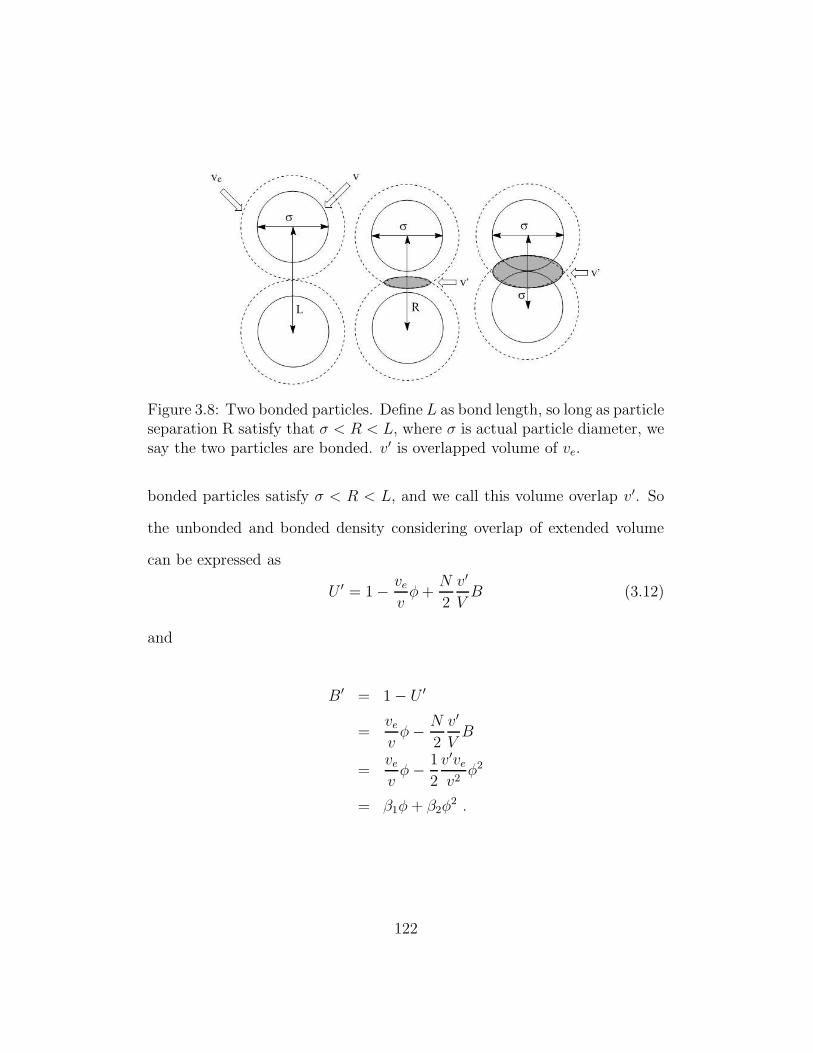
Figure 3.8: Two bonded particles. Define L as bond length, so long as particleseparation R satisfy that σ < R < L, where σ is actual particle diameter, wesay the two particles are bonded. v′ is overlapped volume of ve.
bonded particles satisfy σ < R < L, and we call this volume overlap v′. So
the unbonded and bonded density considering overlap of extended volume
can be expressed as
U ′ = 1 − ve
vφ +
N
2
v′
VB (3.12)
and
B′ = 1 − U ′
=ve
vφ − N
2
v′
VB
=ve
vφ − 1
2
v′ve
v2φ2
= β1φ + β2φ2 .
122
Therefore, we used polynomial fitting B = β0 + β1φ + β2φ2 for our bond
density profiles (such as Figures 3.7 and 3.9), constraining β0 = 0, β1 > 0,
and β2 < 0. In the presence of an external field the actual B will be higher
than that at zero field, so an increasing β1 with increasing field was expected.
The polynomial fit of bond density vs φ profile showed its advantage es-
pecially at Experiment L1 (as shown in Figure 3.9) where a nonlinearity rose
up at high field: At high enough φ (φ ? 20%) particles in a confocal image
appear close to each other and bond density B will reach its maximum at
this point, after where increasing φ will only decrease B. For high fields, not
only the high φ points behave nonlinearly, the points at low φ (φ > 2%) also
increase nonlinearly with φ. The reason for this was due to the stronger dipo-
lar interaction between particles (for 1.14 µm particles) for high field cases
in Experiment L1, as the strength of the interaction was proportional to the
cube of particle diameter. Therefore, very few particles at low φ situation
could still form bonds and led to a high bond density at high enough fields.
In Figure 3.10, we present all the results of β1 vs lambda parameter Λ (de-
scribed in Equation 1.3) from the three experiments to see how β1 behaves in
different fields and if there is any threshold-like behavior. Since each particle
should has the same weight in the curve fitting of bond density profiles, we
used C√
N (where N was the local particle number and C was a constant)
as the weight for the polynomial fit function, producing the same error of
123
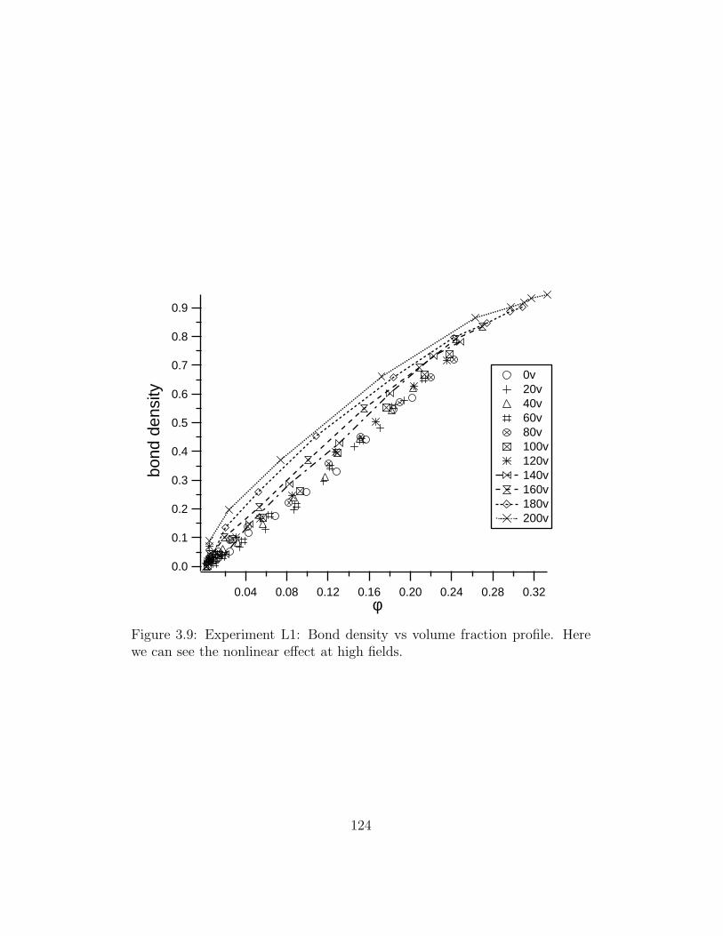
0.9
0.8
0.7
0.6
0.5
0.4
0.3
0.2
0.1
0.0
bond
den
sity
0.320.280.240.200.160.120.080.04φ
0v 20v 40v 60v 80v 100v 120v 140v 160v 180v 200v
Figure 3.9: Experiment L1: Bond density vs volume fraction profile. Herewe can see the nonlinear effect at high fields.
124
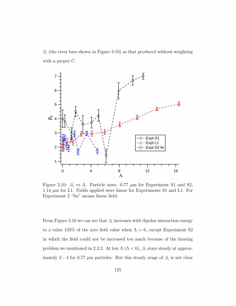
β1 (the error bars shown in Figure 3.10) as that produced without weighting
with a proper C.
7
6
5
4
3
2
1
b1
1612840L
Expt S1 Expt L1 Expt S2 lin
Figure 3.10: β1 vs Λ. Particle sizes: 0.77 µm for Experiment S1 and S2,1.14 µm for L1. Fields applied were linear for Experiments S1 and L1. ForExperiment 2 “lin” means linear field.
From Figure 3.10 we can see that β1 increases with dipolar interaction energy
to a value 150% of the zero field value when Λ > 6, except Experiment S2
in which the field could not be increased too much because of the heating
problem we mentioned in 2.3.2. At low Λ (Λ < 6), β1 stays steady at approx-
imately 2 - 4 for 0.77 µm particles. But this steady stage of β1 is not clear
125
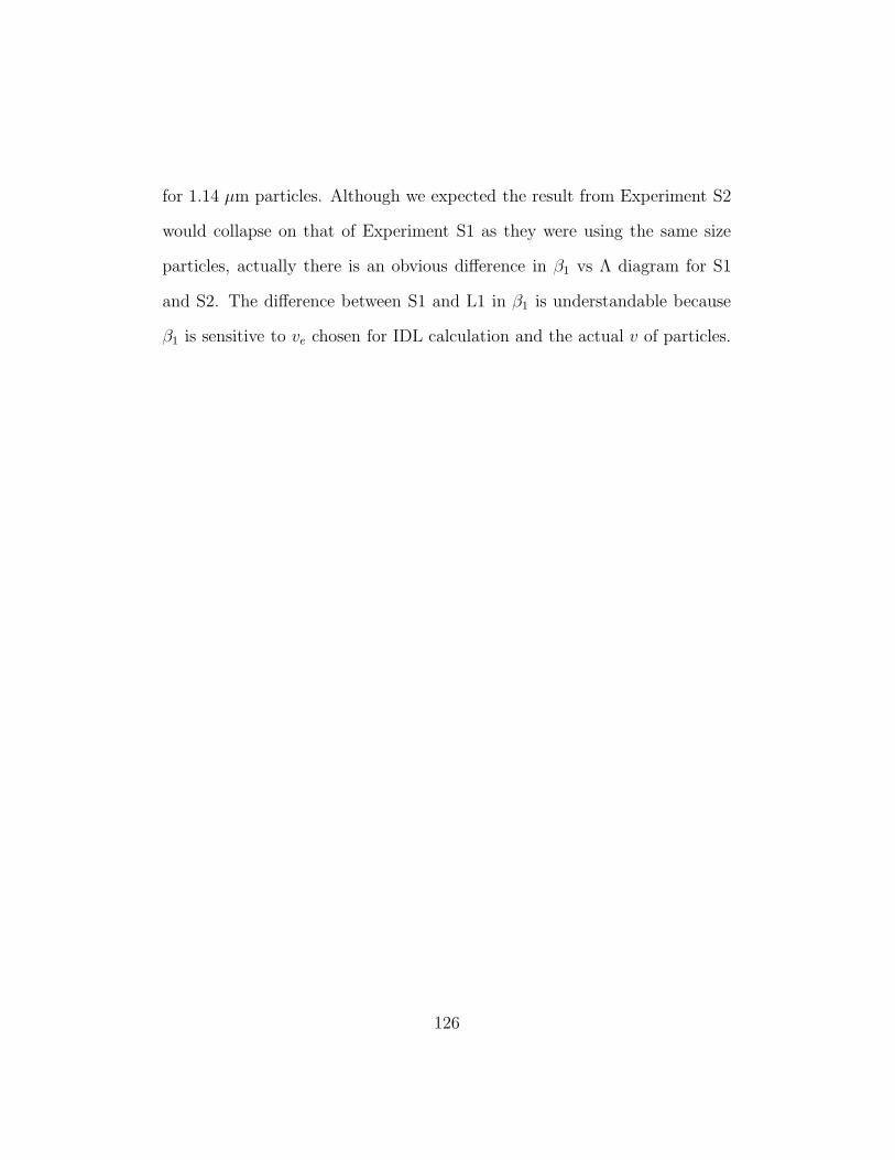
for 1.14 µm particles. Although we expected the result from Experiment S2
would collapse on that of Experiment S1 as they were using the same size
particles, actually there is an obvious difference in β1 vs Λ diagram for S1
and S2. The difference between S1 and L1 in β1 is understandable because
β1 is sensitive to ve chosen for IDL calculation and the actual v of particles.
126
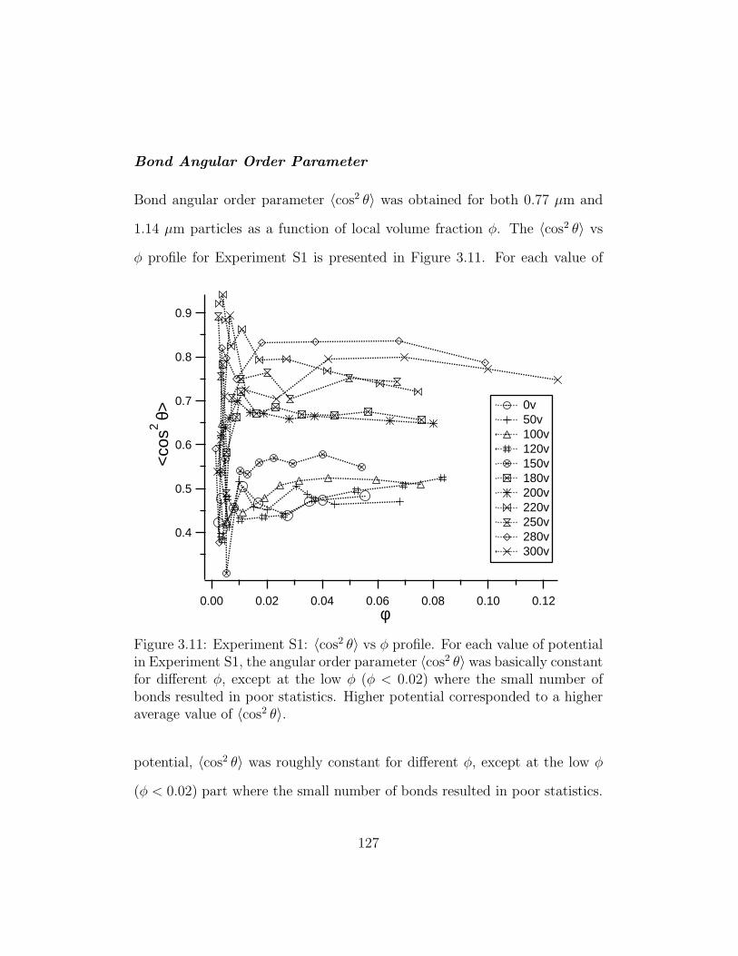
Bond Angular Order Parameter
Bond angular order parameter 〈cos2 θ〉 was obtained for both 0.77 µm and
1.14 µm particles as a function of local volume fraction φ. The 〈cos2 θ〉 vs
φ profile for Experiment S1 is presented in Figure 3.11. For each value of
0.9
0.8
0.7
0.6
0.5
0.4
<co
s2 θ>
0.120.100.080.060.040.020.00φ
0v 50v 100v 120v 150v 180v 200v 220v 250v 280v 300v
Figure 3.11: Experiment S1: 〈cos2 θ〉 vs φ profile. For each value of potentialin Experiment S1, the angular order parameter 〈cos2 θ〉 was basically constantfor different φ, except at the low φ (φ < 0.02) where the small number ofbonds resulted in poor statistics. Higher potential corresponded to a higheraverage value of 〈cos2 θ〉.
potential, 〈cos2 θ〉 was roughly constant for different φ, except at the low φ
(φ < 0.02) part where the small number of bonds resulted in poor statistics.
127
For different potentials, it appeared that higher potential corresponded to a
higher average value of 〈cos2 θ〉, which can be understood because particles
were more likely to form chains parallel to the field direction at higher fields
(〈cos2 θ〉 = 1 for a perfect particle chain, along y axis and parallel to the
linear field).
For larger particles (Figure 3.12), a significant decrease (roughly linear) in
〈cos2 θ〉 is seen at high fields. The reason was closely related to that for the
0.9
0.8
0.7
0.6
0.5
0.4
0.3
<co
s2 θ>
0.400.360.320.280.240.200.160.120.080.04φ
0v 20v 40v 60v 80v 100v 120v 140v 160v 180v 200v
Figure 3.12: Bond angle parameter vs volume fraction profile for ExperimentL1 (1.14 µm): here we can see even at high volume fraction, 〈cos2 θ〉 stillbehaves linearly even the line starts to be tilted at high volume fraction andfield.
128
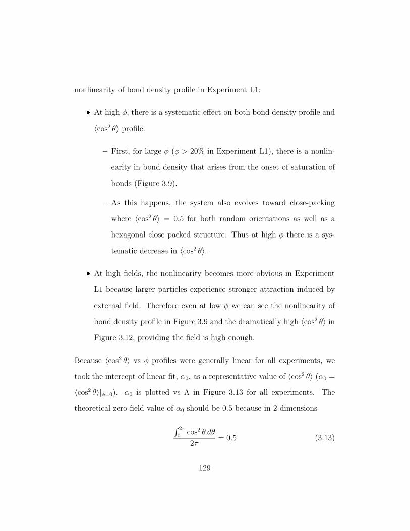
nonlinearity of bond density profile in Experiment L1:� At high φ, there is a systematic effect on both bond density profile and
〈cos2 θ〉 profile.
– First, for large φ (φ > 20% in Experiment L1), there is a nonlin-
earity in bond density that arises from the onset of saturation of
bonds (Figure 3.9).
– As this happens, the system also evolves toward close-packing
where 〈cos2 θ〉 = 0.5 for both random orientations as well as a
hexagonal close packed structure. Thus at high φ there is a sys-
tematic decrease in 〈cos2 θ〉.� At high fields, the nonlinearity becomes more obvious in Experiment
L1 because larger particles experience stronger attraction induced by
external field. Therefore even at low φ we can see the nonlinearity of
bond density profile in Figure 3.9 and the dramatically high 〈cos2 θ〉 in
Figure 3.12, providing the field is high enough.
Because 〈cos2 θ〉 vs φ profiles were generally linear for all experiments, we
took the intercept of linear fit, α0, as a representative value of 〈cos2 θ〉 (α0 =
〈cos2 θ〉|φ=0). α0 is plotted vs Λ in Figure 3.13 for all experiments. The
theoretical zero field value of α0 should be 0.5 because in 2 dimensions
∫ 2π
0cos2 θ dθ
2π= 0.5 (3.13)
129
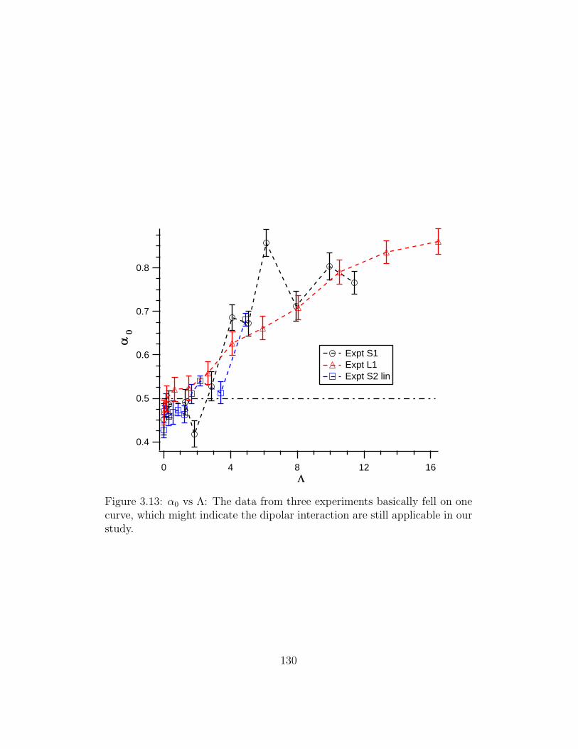
0.8
0.7
0.6
0.5
0.4
a 0
1612840L
Expt S1 Expt L1 Expt S2 lin
Figure 3.13: α0 vs Λ: The data from three experiments basically fell on onecurve, which might indicate the dipolar interaction are still applicable in ourstudy.
130
However, our starting value was always slightly smaller than 0.5 in all 3 ex-
periments, which we do not understand yet.
If the dipolar interaction was applicable in our case, we would expect α0
plotted against the dipolar strength Λ to be independent of particle size, i.e.
the increase of α0 upon Λ from all three linear experiments shall collapse
onto one master curve. Because the orientations of bonds were more parallel
to the field direction as the dipolar energy became stronger. In fact, the
data in Figure 3.13 from linear field experiments of different particle sizes do
collapse onto one curve. This suggests that the point-dipolar approximation
in Equation 1.2 is applicable for the colloids in our study.
For rotating field in Experiment S2, α0 stayed almost steady over the whole
range of applied field energy. This is expected because no direction in the
x-y plane is preferred in a rotating field. There was a slight decrease with
increasing field energy, which is expected because the four electrodes cre-
ating the rotating field were not perfectly symmetric about the center (see
2.3.2) but wider separated in the direction perpendicular to the reference
of θ (i.e. the averaged field direction actually slightly preferred x direction
than y direction). To show the difference between linear and rotating fields
in Experiment S2, we plotted α0 vs 〈E2〉 for this experiment and show it in
Figure 3.14.
131
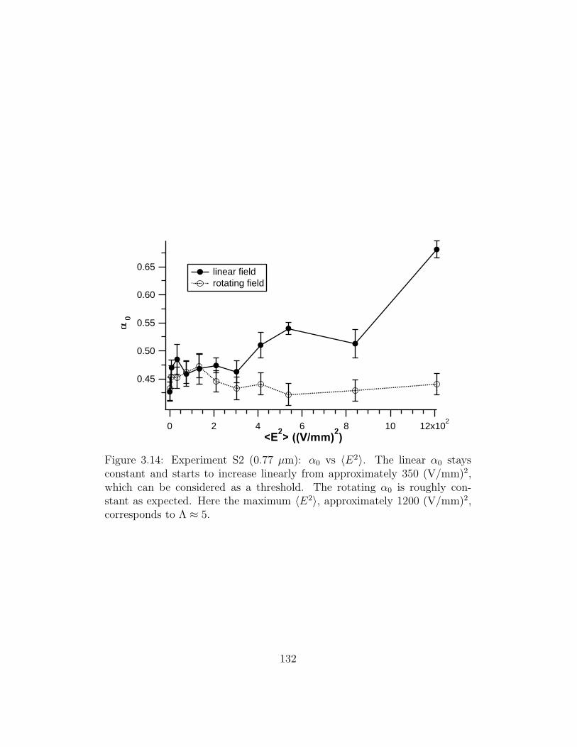
0.65
0.60
0.55
0.50
0.45
a 0
12x102
1086420<E
2> ((V/mm)
2)
linear field rotating field
Figure 3.14: Experiment S2 (0.77 µm): α0 vs 〈E2〉. The linear α0 staysconstant and starts to increase linearly from approximately 350 (V/mm)2,which can be considered as a threshold. The rotating α0 is roughly con-stant as expected. Here the maximum 〈E2〉, approximately 1200 (V/mm)2,corresponds to Λ ≈ 5.
132
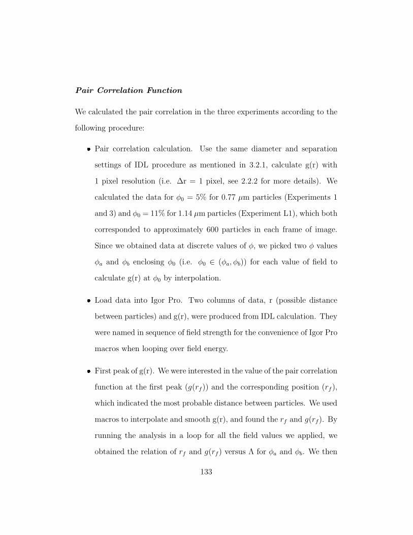
Pair Correlation Function
We calculated the pair correlation in the three experiments according to the
following procedure:� Pair correlation calculation. Use the same diameter and separation
settings of IDL procedure as mentioned in 3.2.1, calculate g(r) with
1 pixel resolution (i.e. ∆r = 1 pixel, see 2.2.2 for more details). We
calculated the data for φ0 = 5% for 0.77 µm particles (Experiments 1
and 3) and φ0 = 11% for 1.14 µm particles (Experiment L1), which both
corresponded to approximately 600 particles in each frame of image.
Since we obtained data at discrete values of φ, we picked two φ values
φa and φb enclosing φ0 (i.e. φ0 ∈ (φa, φb)) for each value of field to
calculate g(r) at φ0 by interpolation.� Load data into Igor Pro. Two columns of data, r (possible distance
between particles) and g(r), were produced from IDL calculation. They
were named in sequence of field strength for the convenience of Igor Pro
macros when looping over field energy.� First peak of g(r). We were interested in the value of the pair correlation
function at the first peak (g(rf)) and the corresponding position (rf ),
which indicated the most probable distance between particles. We used
macros to interpolate and smooth g(r), and found the rf and g(rf). By
running the analysis in a loop for all the field values we applied, we
obtained the relation of rf and g(rf) versus Λ for φa and φb. We then
133

linearly fitted these data for φa and φb, then interpolate in order to
obtain the value for φ0.
Results for Experiment S1 are shown in Figures 3.15 and 3.17. As we in-
creased the field, rf deceased, and g(rf) increased. This is because the inter-
particle attraction becomes stronger, and the particles come closer to each
other when the field energy becomes stronger. The first peak at zero field, as
shown in Figure 3.15, was not sharp, which led to a large and inaccurate rf .
As the field energy was increased, rf was relatively constant at r/σ ≈ 1.6; it
began to decrease toward 1 above Λ ≈ 6. On the other hand, g(rf) stayed
constant at approximately 1.05 - 1.10 and increased to approximately 1.35
at higher fields.
Results for Experiment L1 are shown in Figures 3.16 and 3.17. As we in-
creased the field, rf deceased gradually instead of having a steady range as
Experiment S1, and g(rf) increased after a short steady range at the begin-
ning Λ.
We plot rf and g(rf) vs Λ for all linear experiments in Figures 3.17a and
3.17b. By doing this, we can obtain the general information for all ex-
periments regardless of the different particle size used. There is no other
similarity of rf for Experiments S1 and L1 except both rf collapse to 1 at
134
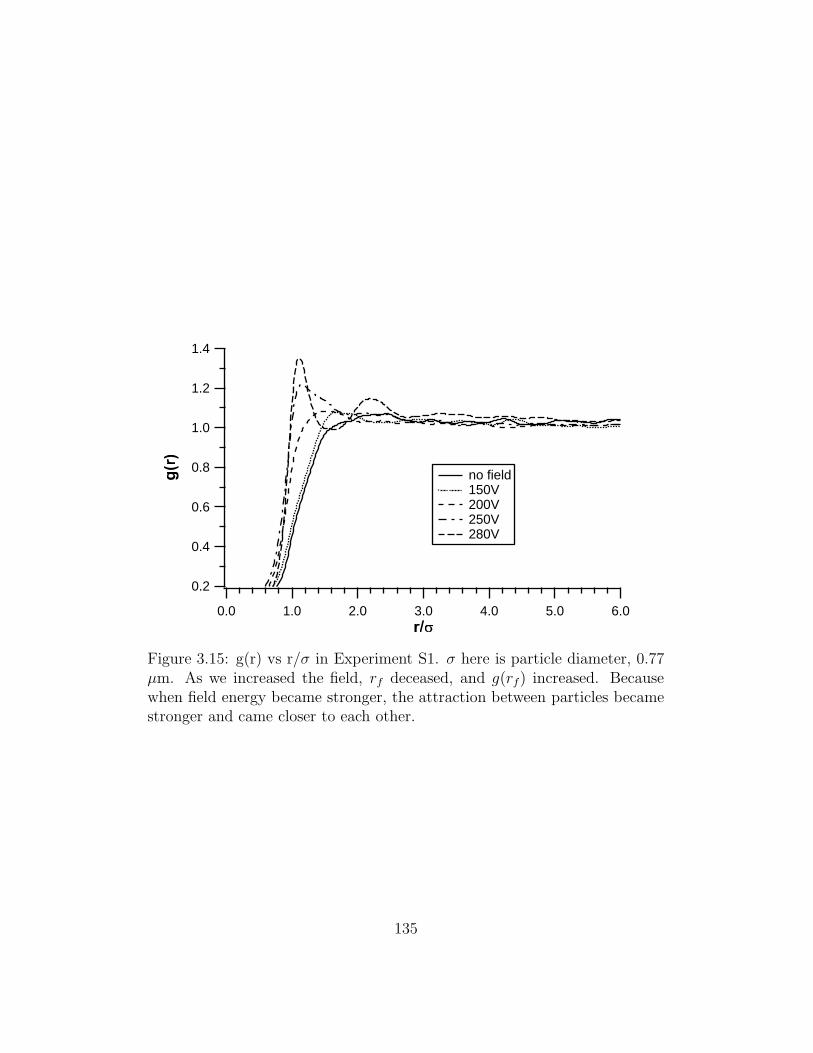
1.4
1.2
1.0
0.8
0.6
0.4
0.2
g(r)
6.05.04.03.02.01.00.0r/s
no field 150V 200V 250V 280V
Figure 3.15: g(r) vs r/σ in Experiment S1. σ here is particle diameter, 0.77µm. As we increased the field, rf deceased, and g(rf) increased. Becausewhen field energy became stronger, the attraction between particles becamestronger and came closer to each other.
135
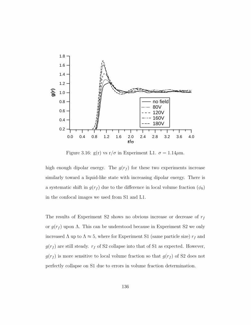
1.8
1.6
1.4
1.2
1.0
0.8
0.6
0.4
0.2
g(r)
4.03.63.22.82.42.01.61.20.80.40.0r/s
no field 80V 120V 160V 180V
Figure 3.16: g(r) vs r/σ in Experiment L1. σ = 1.14µm.
high enough dipolar energy. The g(rf) for these two experiments increase
similarly toward a liquid-like state with increasing dipolar energy. There is
a systematic shift in g(rf) due to the difference in local volume fraction (φ0)
in the confocal images we used from S1 and L1.
The results of Experiment S2 shows no obvious increase or decrease of rf
or g(rf) upon Λ. This can be understood because in Experiment S2 we only
increased Λ up to Λ ≈ 5, where for Experiment S1 (same particle size) rf and
g(rf) are still steady. rf of S2 collapse into that of S1 as expected. However,
g(rf) is more sensitive to local volume fraction so that g(rf) of S2 does not
perfectly collapse on S1 due to errors in volume fraction determination.
136
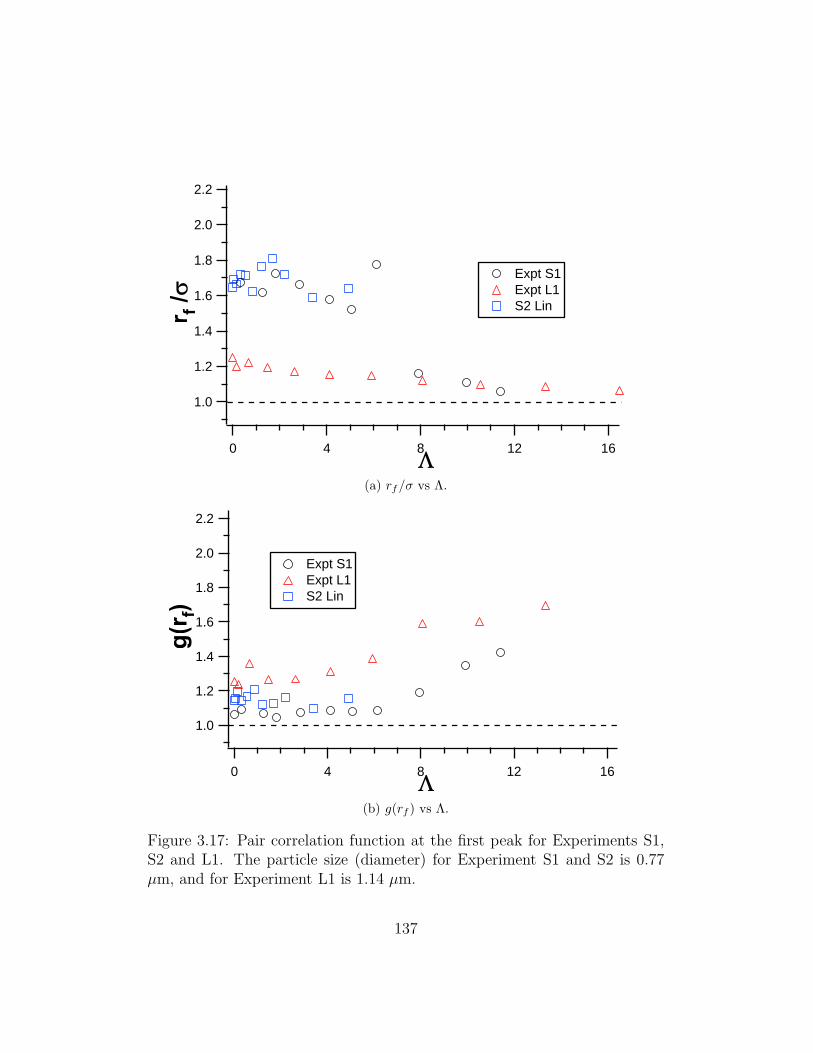
2.2
2.0
1.8
1.6
1.4
1.2
1.0
rf /s
1612840L
Expt S1 Expt L1 S2 Lin
(a) rf/σ vs Λ.
2.2
2.0
1.8
1.6
1.4
1.2
1.0
g(r
f)
1612840L
Expt S1 Expt L1 S2 Lin
(b) g(rf ) vs Λ.
Figure 3.17: Pair correlation function at the first peak for Experiments S1,S2 and L1. The particle size (diameter) for Experiment S1 and S2 is 0.77µm, and for Experiment L1 is 1.14 µm.
137
Osmotic Compressibility
We studied the equilibrium sedimentation profile of colloidal silica particles,
using the vertical density profiles (see 2.2.2 and 3.1.3 for more details), to
calculate isothermal osmotic compressibility of our colloidal system and to
study its dependence on field energy.
In a colloidal silica suspension at sedimentation equilibrium, we can measure
the local particle density n(z), where z is the vertical coordinate measured
from the bottom of the sediment, and from it, calculate the osmotic pressure
of the system Π(z). The osmotic equilibrium condition is [38], [39]
dΠ(z)
dz= −mgn(z) . (3.14)
Under isothermal conditions, Π depends only on n(z), therefore, Equation
3.14 can be written as
dn(z)
dz= −l−1
g χTn(z) , (3.15)
where χT = kBT (∂Π/∂n)−1T is the isothermal osmotic compressibility, and
lg = kBT/mg is the gravitational length. In the dilute gas limit (χT = 1) we
can obtain from Equation 3.15 the barometric law:
n(z) = n0 exp[− z
lg] . (3.16)
138
We rewrite Equation 3.15 as
ln(n(z)) = ln(n0) − z l−1g χT (3.17)
for our analysis below.
The gravitational length lg for 0.77 µm particle is calculated to be 1.92
µm, and for 1.14 µm particle is 0.59 µm, and the estimated error is 14%.
We studied the top part of the sediments (the tail of the density profile
in Figure 3.18), where colloidal particles were few enough to behave like fluid
and we could fit to a exponential curve as Equation 3.16. We linearly fitted
ln φ vs z (as shown in Equation 3.17) instead of direct exponential fitting,
which put more weight for particles at higher φ. φ(z) and number density
n(z) only differ in a constant, i.e. the single particle volume, so they are
equivalent for this purpose.
We obtained the χT from the slope of the linear fitting, plot the χT vs Λ
in Figure 3.19 and observe these effects:� With increasing field, χT increases almost linearly. This can be ex-
plained as: because of increasing field energy, the inter-particle attrac-
tion increases, so the colloids appear to be easier to compress, i.e. a
larger apparent compressibility.
139
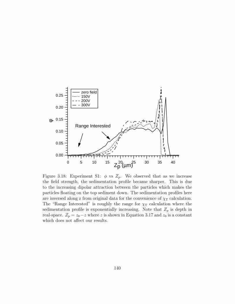
0.25
0.20
0.15
0.10
0.05
0.00
φ
4035302520151050Zp (µm)
Range Interested
zero field 150V 200V 300V
Figure 3.18: Experiment S1: φ vs Zp. We observed that as we increasethe field strength, the sedimentation profile became sharper. This is dueto the increasing dipolar attraction between the particles which makes theparticles floating on the top sediment down. The sedimentation profiles hereare inversed along z from original data for the convenience of χT calculation.The “Range Interested” is roughly the range for χT calculation where thesedimentation profile is exponentially increasing. Note that Zp is depth inreal-space. Zp = z0−z where z is shown in Equation 3.17 and z0 is a constantwhich does not affect our results.
140
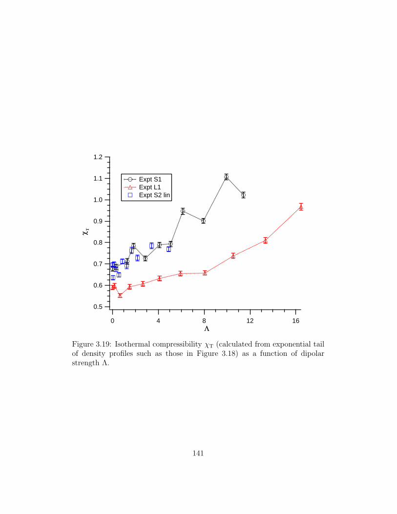
1.2
1.1
1.0
0.9
0.8
0.7
0.6
0.5
cT
1612840L
Expt S1 Expt L1 Expt S2 lin
Figure 3.19: Isothermal compressibility χT (calculated from exponential tailof density profiles such as those in Figure 3.18) as a function of dipolarstrength Λ.
141
� At zero field, all χT are smaller than 1, which means our systems cannot
be considered as ideal gas or hard spheres at low φ. Softness (i.e. the
repulsion in interaction potential) is a possible reason for the decrease of
χT. Although our systems are very close to hard spheres (κ−1 ≈ 50nm),
deviations from ideal hard-sphere behaviors can cause small decrease
in χT. Indeed these deviations are also observed in the position of the
first peak of the pair correlation functions being much larger than 1
(i.e. rf/σ > 1).� χT for 1.14 µm particles is systematically smaller than that for 0.77
µm particles. This is reasonable because at a given number density,
the effective hard-sphere repulsion is more important for larger spheres,
which can make the colloidal system more difficult to compress, i.e. a
smaller χT.� The error in the determination of particle size (within 5%) and material
density can cause systematic error in the gravitational length lg, which
can affect our calculation.
142
3.3 Conclusions
In this thesis, we have synthesized fluorescent-labeled colloids, constructed
samples and software for confocal microscopy experiments, and conducted
experiments where we study the behavior of quiescent colloidal sediments as
well as the response of the colloidal suspension to and external electric field.
In the studies of quiescent colloidal sedimentation profiles, we observed un-
expected plateau region (Figure 3.18). A further analysis of the exponential
region of these sedimentation profiles showed that the values of the isother-
mal osmotic compressibility χT at zero-field were smaller than 1 for both
0.77 µm and 1.14 µm colloids (Figure 3.19), which indicated that our sys-
tems were not perfectly hard-sphere like.
Next, we studied colloidal ordering in the presence of a high-frequency (MHz)
AC field of variable strength characterized by a dipolar strength parameter
Λ (because we assumed a dipolar inter-particle interaction). For our electric
field studies, we used not only the pair correlation functions but also, various
bond order parameters, and isothermal osmotic compressibility, which helped
us to quantify field-induced structure. We did not know beforehand which
order parameter would give us the most information. We tried two bond
order parameters (bond density and bond angular parameters) as described
below.
143
The bond density parameter β1: The plot of the bond density param-
eter β1 vs the dipolar energy parameter Λ diagram (Figure 3.10) exhibits a
steady low field value for 0.77 µm experiments (S1 and S2). At high Λ, β1
in both Experiments S1 and L1 rises to approximately 150% of the zero field
value. We were unable to increase the rotating field to a high value due to
sample-heating problems, so there is no high field data for Experiment S2.
β1 from all experiments did not collapse into one curve, but this is expected
as β1 is sensitive to the parameters chosen for bond density calculation; these
parameters vary a bit from experiment to experiment.
The bond angular parameter α0: The extrapolation of φ-dependence
of 〈cos2 θ〉 to zero φ, α0, turned out to be a self-consistent way to compare
all experiment and superior to the bond density parameter β1. For exper-
iments where the 〈cos2 θ〉 vs φ profiles were flat, α0 was also close to the
average 〈cos2 θ〉. But we used α0 instead of average 〈cos2 θ〉 because α0 is
less sensitive to the shape of 〈cos2 θ〉 vs φ profiles. We note the following:� For linear fields, α0 increases from random bond-orientation (α0 ≈ 0.5)
to highly anisotropic along the field direction (α0 > 0.8). All linear
experiments (different particle sizes) had α0 vs Λ curves that collapsed
onto one master curve (Figure 3.13). This is a strong indication that, at
least at these field values, the dipolar approximation is valid. Moreover,
the Λ parameter at the onset for chain formation is approximately 6
144
instead of 1. Thus although the dipolar approximation is valid, we
must still view it as an effective dipolar interaction.� For rotating fields, bond orientation was absent as expected, causing
α0 to be different from linear field results in the same sample (Figure
3.14).
In summary, we found that while β1 was very sensitive to software parame-
ters, α0 was a robust parameter that accurately reflected colloidal response to
an electric field. When plotted against a dipolar strength parameter (which
has all particle size dependence absorbed), results for different particle sizes
fall on one curve. This suggests strongly the validity of the dipolar interac-
tion. Moreover, we proved that we can switch the colloidal system between
anisotropic phase and isotropic phase by switching the external electric field
directions between linear and rotating.
The pair correlation function g(r): The results from pair correlation
function calculation supported that as field energy increases, more parti-
cles come closer to each other due to the increased inter-particle attraction.
The position of the first peak of g(r), rf , approached the particle diameters,
i.e. rf/σ → 1, as the external field was increased. The magnitude of g(rf)
also increased with field, with the structure approaching liquid-like behaviors
(Figure 3.17).
145

The isothermal compressibility χT: In the presence of an external high-
frequency AC field, χT increased dramatically at moderate values of Λ (Fig-
ure 3.19). Increase in χT is reasonable: increasing Λ increases dipole-dipole
interaction which compresses the colloidal sediment.
146
Outlook
The experiments described in this thesis quantify colloid structure at low
volume fractions in the presence of gravity and low electric fields. First,
the measurements presented make quantitative statements about structure
in a quiescent colloidal sediment. Several questions remain to be definitively
answered:� What causes the plateau region? We already know that there must
be an inter-particle repulsion (from pair correlation as well as the less-
than-unity zero-field value of χT). Could this cause the plateau region
or must van der Waals attraction be taken into account? Comparison
of experiments with computer simulations currently under way could
shed light on this.� Why is the isothermal compressibility χT at zero field lower than unity?
The could be caused by the softness of the zero-field interaction poten-
tial. While we estimated κ−1 < 50 nm, we nevertheless observed that
the first peak of pair correlation function g(r) was at rf/σ ≈ 1.6 for
0.77 µm diameter colloidal particles. It is reasonable that softness de-
creases compressibility: again a comparison with simulation would be
interesting.
Second, while the field-induced structure appears to be consistent with dipo-
lar interaction, it is nevertheless curious that colloids feel the presence of the
147

electric field at Λ ≈ O(10) rather than O(1).
Finally, we successfully tested modification of interactions in a rotating elec-
tric field. But we still have problem to solve such as:� modify cell to achieve higher fields,� study phase behavior in rotating fields.
148

Bibliography
[1] W. B. Russel, D. A. Saville, and W. R. Schowalter. Colloidal Disper-
sions. Cambridge University Press, 1989.
[2] D. Fennell Evans and H. Wennerstrom. The Colloidal Domain: Where
Physics, Chemistry, Biology, and Technology Meet. Advances in Inter-
facial Engineering. VCH, 1994.
[3] A. Vrij, E. A. Nieuwenhuis, H. M. Fijnaut, and W. G. M. Agterof.
Application of modern concepts in liquid state theory to concentrated
particle dispersions. Faraday Discuss., 65:101–113, 1978.
[4] P. N. Pusey and W. van Megen. Phase behaviour of concentrated sus-
pensions of nearly hard colloidal spheres. Nature, 320:340–342, 1986.
[5] P. N. Pusey and W. van Megen. Observation of a glass transition in sus-
pensions of spherical colloidal particles. Phys. Rev. Lett., 59(18):2083–
2086, 1987.
149
[6] V. Prasad, D. Semwogerere, and E. Weeks. Confocal microscopy of
colloids. J. Phys.: Condens. Matter, 19, 2007.
[7] T. G. M. van de Ven. Colloidal Hydrodynamics. Colloid Science. Aca-
demic Press, 1988.
[8] H.C. Hamaker. The London – van der Waals attraction between spher-
ical particles. Physica, 4(10):1058–1072, 1937.
[9] Malvern Instruments Website. http://www.malvern.com /labeng /in-
dustry /colloids /dlvo theory.htm.
[10] A. Hynninen and M. Dijkstra. Phase behavior of dipolar hard and soft
spheres. Phys. Rev. E, 72(5), 2005.
[11] A. Yethiraj. Tunable colloids: control of colloidal phase transitions with
tunable interactions. Soft Matter, 3:1099–1115, 2007.
[12] R. Tao, J. T. Woestman, and N. K. Jaggi. Electric field induced solidi-
fication. Appl. Phys. Lett., 55(18):1844–1846, 1989.
[13] R. Tao and J. M. Sun. Three-dimensional structure of induced elec-
trorheological solid. Phys. Rev. Lett., 67(3):398–401, 1991.
[14] R. Tao and J. M. Sun. Ground state of electrorheological fluids from
monte carlo simulations. Phys. Rev. A, 44(10):R6181–R6184, 1991.
150
[15] T. Chen, R. N. Zitter, and R. Tao. Laser diffraction determination of
the crystalline structure of an electrorheological fluid. Phys. Rev. Lett.,
68(16):2555–2558, 1992.
[16] U. Dassanayake, S. Fraden, and A. van Blaaderen. Structure of elec-
trorheological fluids. J. Chem. Phys., 112(8):3851–3858, 2000.
[17] A. Yethiraj and A. van Blaaderen. A colloidal model system with an in-
teraction tunable from hard sphere to soft and dipolar. Nature, 421:513–
517, 2003.
[18] A. Yethiraj, A. Wouterse, B. Groh, and A. van Blaaderen. Nature of an
electric-field-induced colloidal martensitic transition. Phys. Rev. Lett.,
92(5), 2004.
[19] S. Fraden, A. J. Hurd, and R. B. Meyer. Electric-field-induced associa-
tion of colloidal particles. Phys. Rev. Lett., 63(21):2373–2376, 1989.
[20] G. Bossis, C. Metayer, and A. Zubarev. Analysis of chaining structures
in colloidal suspensions subjected to an electric field. Phys. Rev. E,
67(041401), 2007.
[21] J. C. van der Werff and C. G. de Kruif. Hard-sphere colloidal dispersions:
The scaling of rheological properties with particle size, volume fraction,
and shear rate. J. Rheol., 33(3):421–454, 1989.
151
[22] T. G. Mason and D. A. Weitz. Optical measurements of frequency-
dependent linear viscoelastic moduli of complex fluids. Phys. Rev. Lett.,
74(7):1250–1253, 1995.
[23] J. C. Crocker, M. T. Valentine, E. R. Weeks, T. Gisler, P. D. Kaplan,
A. G. Yodh, and D. A. Weitz. Two-point microrheology of inhomoge-
neous soft materials. Phys. Rev. Lett., 85(4):888–891, 2000.
[24] J. Hoogenboom. Colloidal Epitaxy: A Real-Space Analysis. PhD thesis,
Universiteit Utrecht, 2002.
[25] M. Born and E. Wolf. Principles of Optics. Cambridge U. Press, Cam-
bridge, 7th expanded edition, 1999.
[26] W. Stober, A. Fink, and E. Bohn. Controlled growth of monodisperse
silica spheres in micron size range. J. Colloid Interface Sci., 26(62),
1968.
[27] H. Giesche. Synthesis of monodispersed silica powders i: particle prop-
erties and reaction kinetics. J. Eur. Ceram. Soc., 14(3):189–204, 1994.
[28] H. Giesche. Synthesis of monodispersed silica powders ii: controlled
growth reactions and continuous production processes. J. Eur. Ceram.
Soc., 14(3):205–214, 1994.
[29] D. ’t Hart. Inverse silicon air sphere photonic crystals. Chapter 3: Syn-
thesis of silica colloids. Master’s thesis, Utrecht University, January
2004.
152
[30] A. van Blaaderen and A. Vrij. Synthesis and characterization of colloidal
dispersions of fluorescent monodisperse silica spheres. Langmuir, 8:2921–
2931, 1992.
[31] J. W. Zubrick. The Organic Chem Lab Survival Manual. John Wiley &
Sons, Inc., sixth edition, 2004.
[32] N. A. M. Verhaegh and A. van Blaaderen. Dispersions of rhodamine-
labeled silica spheres - synthesis, characterization, and fluorescence con-
focal scanning laser microscopy. Langmuir, 10:1427–1438, 1994.
[33] Mandel Scientific Company Inc. http://www.mandel.ca/products/ liq-
uid handling/pumps tubing/tubing/index.htm.
[34] Solutions At Work For You. Minipuls 3 Peristaltic Pump User’s Guide.
Gilson.
[35] J. Crocker and D. Grier. Methods of digital video microscopy for col-
loidal studies. J. Colloid Interface Sci., 179:298–310, 1996.
[36] J. Crocker and E. Weeks. http://www.physics.emory.edu/∼weeks/
idl/index.html.
[37] J. O’M. Bockris and A. K. N. Reddy. Modern Electrochemistry, vol-
ume 1. Plenum Press, second edition, 1998.
153
[38] R. Piazza, T. Bellini, and V. Degiorgio. Equilibrium sedimentation pro-
files of screened charged colloids - a test of the hard-sphere equation of
state. Phys. Rev. Lett., 71(25):4267–4270, 1993.
[39] V. Degiorgio, R. Piazza, and T. Bellini. Depolarized light-scattering
study of equilibrium sedimentation profiles of colloidal dispersions.
Nuovo Cimento D, 16(8):1091–1101, 1994.
154

Appendix A
IDL procedures
155
Appendix B
Igor Pro procedures
175