Embed Size (px)
Citation preview

Collision Avoidance System at Intersections
FINAL REPORT - FHWA-OK-09-06 ODOT SPR ITEM NUMBER 2216
By
Fadi Basma
Research Assistant
Hazem H. Refai Associate Professor
Electrical and Computer Engineering Department The University of Oklahoma
Tulsa, Oklahoma 74135
Technical Advisors: Harold Smart, Traffic Engineering Division Head
December 2009
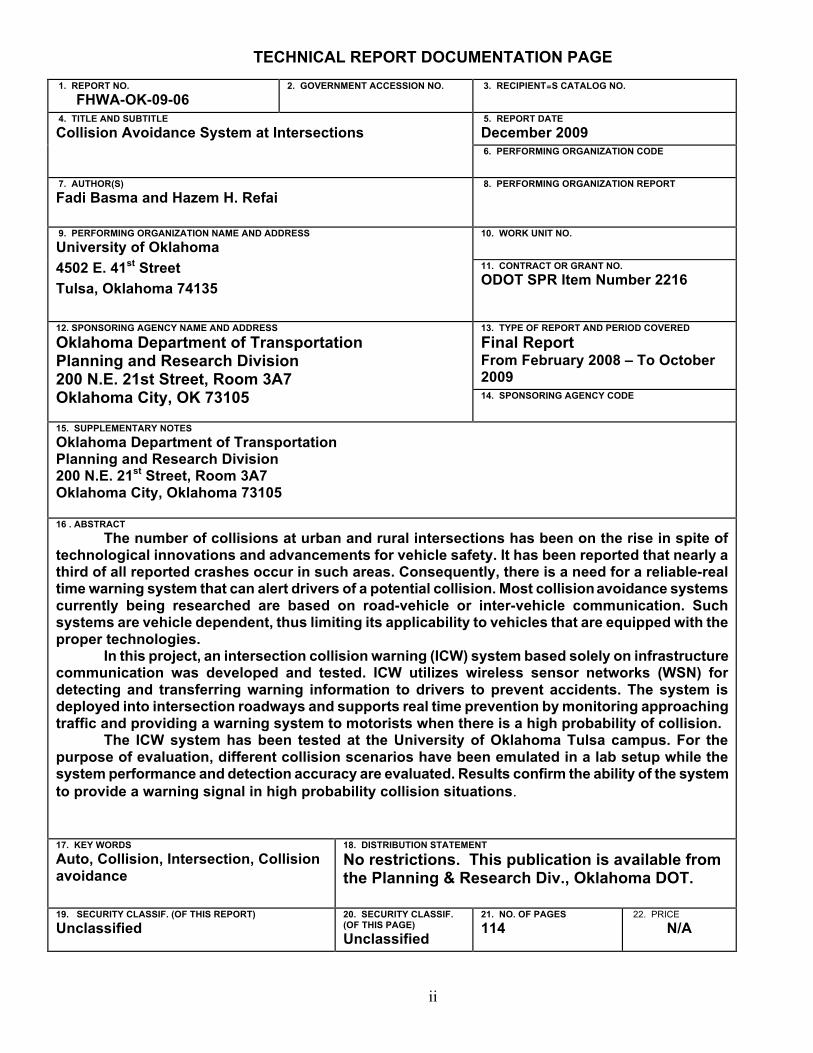
TECHNICAL REPORT DOCUMENTATION PAGE
1. REPORT NO. FHWA-OK-09-06
2. GOVERNMENT ACCESSION NO. 3. RECIPIENT=S CATALOG NO.
4. TITLE AND SUBTITLE Collision Avoidance System at Intersections
5. REPORT DATE December 2009 6. PERFORMING ORGANIZATION CODE
7. AUTHOR(S) Fadi Basma and Hazem H. Refai
8. PERFORMING ORGANIZATION REPORT
9. PERFORMING ORGANIZATION NAME AND ADDRESS University of Oklahoma 4502 E. 41st Street Tulsa, Oklahoma 74135
10. WORK UNIT NO.
11. CONTRACT OR GRANT NO. ODOT SPR Item Number 2216
12. SPONSORING AGENCY NAME AND ADDRESS
Oklahoma Department of Transportation Planning and Research Division 200 N.E. 21st Street, Room 3A7 Oklahoma City, OK 73105
13. TYPE OF REPORT AND PERIOD COVERED
Final Report From February 2008 – To October 2009 14. SPONSORING AGENCY CODE
15. SUPPLEMENTARY NOTES Oklahoma Department of Transportation Planning and Research Division 200 N.E. 21st Street, Room 3A7 Oklahoma City, Oklahoma 73105
16 . ABSTRACT The number of collisions at urban and rural intersections has been on the rise in spite of
technological innovations and advancements for vehicle safety. It has been reported that nearly a third of all reported crashes occur in such areas. Consequently, there is a need for a reliable-real time warning system that can alert drivers of a potential collision. Most collision avoidance systems currently being researched are based on road-vehicle or inter-vehicle communication. Such systems are vehicle dependent, thus limiting its applicability to vehicles that are equipped with the proper technologies.
In this project, an intersection collision warning (ICW) system based solely on infrastructure communication was developed and tested. ICW utilizes wireless sensor networks (WSN) for detecting and transferring warning information to drivers to prevent accidents. The system is deployed into intersection roadways and supports real time prevention by monitoring approaching traffic and providing a warning system to motorists when there is a high probability of collision.
The ICW system has been tested at the University of Oklahoma Tulsa campus. For the purpose of evaluation, different collision scenarios have been emulated in a lab setup while the system performance and detection accuracy are evaluated. Results confirm the ability of the system to provide a warning signal in high probability collision situations.
17. KEY WORDS Auto, Collision, Intersection, Collision avoidance
18. DISTRIBUTION STATEMENT
No restrictions. This publication is available from the Planning & Research Div., Oklahoma DOT.
19. SECURITY CLASSIF. (OF THIS REPORT) Unclassified
20. SECURITY CLASSIF. (OF THIS PAGE) Unclassified
21. NO. OF PAGES 114
22. PRICE
N/A
ii
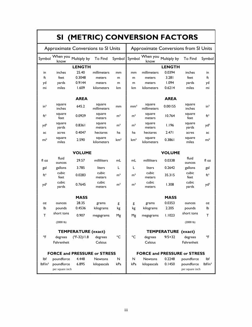
SI (METRIC) CONVERSION FACTORS Approximate Conversions to SI Units Approximate Conversions from SI Units
Symbol When you know
Multiply by To Find Symbol Symbol When you know
Multiply by To Find Symbol
LENGTH in inches 25.40 millimeters mm ft feet 0.3048 meters m yd yards 0.9144 meters m mi miles 1.609 kilometers km
AREA
in² square inches
645.2 square
millimeters mm
ft² square
feet 0.0929 square meters m²
yd² square yards 0.8361
square meters m²
ac acres 0.4047 hectares ha
mi² square miles
2.590 square
kilometers km²
VOLUME
fl oz fluid
ounces 29.57 milliliters mL
gal gallons 3.785 liters L
ft³ cubic feet 0.0283
cubic meters m³
yd³ cubic yards 0.7645
cubic meters m³
LENGTH mm millimeters 0.0394 inches in m meters 3.281 feet ft m meters 1.094 yards yd km kilometers 0.6214 miles mi
AREA
mm² square
millimeters 0.00155
square inches
in²
m² square meters 10.764
square feet ft²
m² square meters 1.196
square yards yd²
ha hectares 2.471 acres ac
km² square
kilometers 0.3861
square miles
mi²
VOLUME
mL milliliters 0.0338 fluid
ounces fl oz
L liters 0.2642 gallons gal
m³ cubic
meters 35.315 cubic feet ft³
m³ cubic
meters 1.308 cubic yards yd³
MASS oz ounces 28.35 grams g lb pounds 0.4536 kilograms kg
T short tons 0.907 megagrams Mg
(2000 lb)
TEMPERATURE (exact) ºF degrees (ºF-32)/1.8 degrees ºC
Fahrenheit Celsius
FORCE and PRESSURE or STRESS lbf poundforce 4.448 Newtons N
lbf/in² poundforce 6.895 kilopascals kPa per square inch
MASS g grams 0.0353 ounces oz kg kilograms 2.205 pounds lb
Mg megagrams 1.1023 short tons T
(2000 lb)
TEMPERATURE (exact) ºC degrees 9/5+32 degrees ºF
Celsius Fahrenheit
FORCE and PRESSURE or STRESS N Newtons 0.2248 poundforce lbf
kPa kilopascals 0.1450 poundforce lbf/in² per square inch
iii
The contents of this report reflect the views of the author(s) who is responsible for the facts and the accuracy of the data presented herein. The contents do not necessarily reflect the views of the Oklahoma Department of Transportation or the Federal Highway Administration. This report does not constitute a standard, specification, or regulation. While trade names may be used in this report, it is not intended as an endorsement of any machine, contractor, process, or product.
v
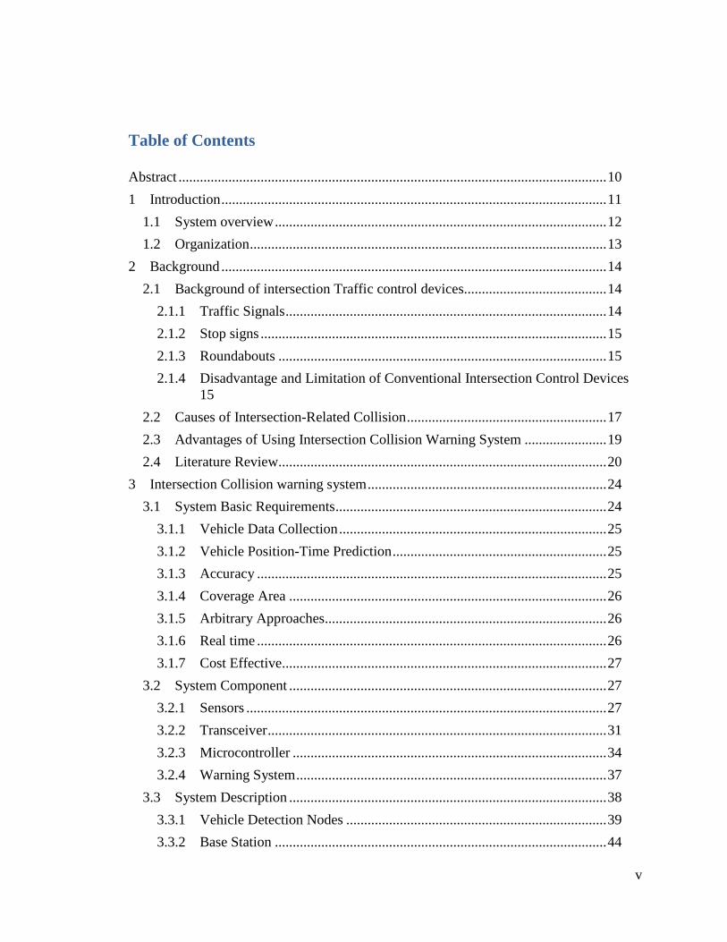
Table of Contents
Abstract ........................................................................................................................ 10 1 Introduction ............................................................................................................ 11
1.1 System overview ............................................................................................. 12 1.2 Organization .................................................................................................... 13
2 Background ............................................................................................................ 14 2.1 Background of intersection Traffic control devices........................................ 14
2.1.1 Traffic Signals .......................................................................................... 14 2.1.2 Stop signs ................................................................................................. 15 2.1.3 Roundabouts ............................................................................................ 15 2.1.4 Disadvantage and Limitation of Conventional Intersection Control Devices 15
2.2 Causes of Intersection-Related Collision ........................................................ 17 2.3 Advantages of Using Intersection Collision Warning System ....................... 19 2.4 Literature Review............................................................................................ 20
3 Intersection Collision warning system ................................................................... 24 3.1 System Basic Requirements ............................................................................ 24
3.1.1 Vehicle Data Collection ........................................................................... 25 3.1.2 Vehicle Position-Time Prediction ............................................................ 25 3.1.3 Accuracy .................................................................................................. 25 3.1.4 Coverage Area ......................................................................................... 26 3.1.5 Arbitrary Approaches............................................................................... 26 3.1.6 Real time .................................................................................................. 26 3.1.7 Cost Effective........................................................................................... 27
3.2 System Component ......................................................................................... 27 3.2.1 Sensors ..................................................................................................... 27 3.2.2 Transceiver ............................................................................................... 31 3.2.3 Microcontroller ........................................................................................ 34 3.2.4 Warning System ....................................................................................... 37
3.3 System Description ......................................................................................... 38 3.3.1 Vehicle Detection Nodes ......................................................................... 39 3.3.2 Base Station ............................................................................................. 44
vi
3.3.3 Warning System ....................................................................................... 46 3.4 Wireless Communication ................................................................................ 48
3.4.1 Modulation ............................................................................................... 48 3.4.2 Bandwidth ................................................................................................ 48 3.4.3 Interference .............................................................................................. 48 3.4.4 Range ....................................................................................................... 48 3.4.5 MAC ........................................................................................................ 49 3.4.6 Network Capacity .................................................................................... 50 3.4.7 Error Detection......................................................................................... 50
4 System Processing ................................................................................................. 51 4.1 Oscillator Select .............................................................................................. 51 4.2 Interfacing ....................................................................................................... 51
4.2.1 Universal Asynchronous Receiver Transmitter ....................................... 52 4.2.2 Parallel Master Port (PMP) ...................................................................... 56 4.2.3 Digital I/O port ......................................................................................... 59
4.3 Interrupts ......................................................................................................... 59 4.3.1 Power Efficiency Methodology ............................................................... 61 4.3.2 Wi232DTS Network Routing .................................................................. 61 4.3.3 Power consumption .................................................................................. 62 4.3.4 Sleep Mode .............................................................................................. 64
4.4 Vehicle Trajectory Prediction ......................................................................... 66 4.5 Time Synchronization ..................................................................................... 68
4.5.1 Clock implementation .............................................................................. 68 4.5.2 Time Synchronization .............................................................................. 70
4.6 System Detection ............................................................................................ 78 4.7 Intersection Collision Avoidance and Warning System ................................. 86 4.8 Overall ICW System ....................................................................................... 87 4.9 Packets Structure ............................................................................................. 89
5 Simulation and Testing .......................................................................................... 93 5.1 Kalman Filter Vs 2nd Order motion ................................................................ 93 5.2 Overall System Latency .................................................................................. 97
5.2.1 Analysis and Results ................................................................................ 97 5.3 Bit Error Rate Vs Distance ............................................................................. 98
5.3.1 Testing Setup ........................................................................................... 98

vii
5.3.2 Analysis and Results .............................................................................. 102 5.4 System Collision detection performance ...................................................... 103
5.4.1 Testing Setup ......................................................................................... 104 5.4.2 Analysis and Results .............................................................................. 109
6 REFERENCES .................................................................................................... 111
viii
LIST OF FIGURES
Figure 1: Overview of ICW ......................................................................................... 12Figure 2: Distribution of common accident situations [10] ......................................... 18Figure 3: Intersection collision warning system phases .............................................. 24Figure 4: Sensor comparison [29] ................................................................................ 28Figure 5: Magnetic anomaly in the Earth’s magnetic field induced by magnetic dipoles in a ferrous metal vehicle [29] ......................................................................................... 30Figure 6: Vehicle detection sensor schematic [31] ...................................................... 31Figure 7: Measured sensor voltage from vehicle disturbance [31] .............................. 31Figure 8: WiSE block diagram [33] ............................................................................. 33Figure 9: Warning signal displayed by TM162JCAWG1 LCD .................................. 38Figure 10: ICW design description .............................................................................. 39Figure 11: Vehicle detection node decomposition ....................................................... 41Figure 12: Base station decomposition ........................................................................ 45Figure 13: Warning system decomposition ................................................................. 47Figure 14: Non-persistent CSMA ................................................................................ 50Figure 15: Simplified UART module interface between the microcontroller and the wireless transceiver ...................................................................................................... 53Figure 16: PMP module overview ............................................................................... 57Figure 17: Detection node sleep mode logic ................................................................ 65Figure 18: Detailed description of the system prediction algorithm ............................ 68Figure 19: Logic to achieve a millisecond rang ........................................................... 69Figure 20: Basic logic for detection node .................................................................... 74Figure 21: Time synchronizing logic for the Base Station .......................................... 77Figure 22: Detection node vehicle detection logic ...................................................... 80Figure 23: Example of BS group buffers representation in a three second margin ..... 82Figure 24: BS vehicle detection logic .......................................................................... 85Figure 25: Representation of two vehicles entering and exiting the intersection ........ 86Figure 26: Intersection collision avoidance and warning System logic ...................... 87Figure 27: BS overall software logic ........................................................................... 88Figure 28: Detection node overall software logic ........................................................ 89Figure 29: ICW Packets Structure ............................................................................... 92Figure 30: Predicted distance without errors (sampling rate=0.001, vi=20.1168 m/s, acceleration=-1m/𝒔𝒔𝒔𝒔) ................................................................................................... 95 Figure 31: Predicted distance with errors (sampling rate=0.001, vi=20.1168 m/s, acceleration=-1m/𝒔𝒔𝒔𝒔 .................................................................................................... 96 Figure 32: Transceivers placement for setup 1 and 2 ................................................ 101Figure 33: Transceivers placement for setup 3 .......................................................... 101Figure 34: System transmission BER ........................................................................ 103Figure 35: Collision detection testing Setup .............................................................. 108
ix
LIST OF TABLES
Table 1: Intersection-related collision source description ........................................... 19Table 2: Candidate transceivers ................................................................................... 32Table 3: Feature summary for WI.232DTS module .................................................... 34Table 4: Expected microcontroller features ................................................................. 35Table 5: PIC24FJ128GA010 features [37] .................................................................. 37Table 6: Stopping distance value range [10] ................................................................ 43Table 7: Current/Power consumption for system components .................................... 63Table 8: ICW solutions for detection issues ................................................................ 78Table 9: ICW system latency ....................................................................................... 98Table 10: Collision detection testing results .............................................................. 110

10
Abstract
The number of collisions at urban and rural intersections has been on the rise in spite of
technological innovations and advancements for vehicle safety. It has been reported that nearly a
third of all reported crashes occur in such areas. Consequently, there is a need for a reliable-real
time warning system that can alert drivers of a potential collision. Most collision avoidance
systems currently being researched are based on road-vehicle or inter-vehicle communication.
Such systems are vehicle dependent, thus limiting its applicability to vehicles that are equipped
with the proper technologies.
In this project, an intersection collision warning (ICW) system based solely on
infrastructure communication was developed and tested. ICW utilizes wireless sensor networks
(WSN) for detecting and transferring warning information to drivers to prevent accidents. The
system is deployed into intersection roadways and supports real time prevention by monitoring
approaching traffic and providing a warning system to motorists when there is a high probability
of collision.
The ICW system has been tested at the University of Oklahoma Tulsa campus. For the
purpose of evaluation, different collision scenarios have been emulated in a lab setup while the
system performance and detection accuracy are evaluated. Results confirm the ability of the
system to provide a warning signal in high probability collision situations.
11
1 Introduction
Each year there have been over 40,000 fatalities and 2,788,000 non-fatal injuries due
to traffic accidents in the United States [1]. In addition, it is predicted that hospital bills,
damaged properties and additional accident-related costs will add up to approximately
one to three percent of the world’s gross domestic product [2][3]. Accordingly,
developing a collision warning system that is capable of preventing accidents regardless
of unexpected conditions is of great importance.
Although there have been a number of technological innovations in vehicle safety,
the number of accidents continues to rise. This is especially true for intersection
accidents. It has been reported that nearly 30% of the reported accidents in the United
States are due to intersection collision [4] [5]. Most of these accidents take place at rural
intersection areas equipped with traffic signals or stop signs. As a result, it is
recommended that an intersection collision warning system be implemented as a part of
vehicle safety systems, thus reducing the number of accidents. To be most effective, such
a system should have the capability of supporting real time systems that can warn
potential drivers of an impending collision. It also should be adaptable to different types
of intersections.
This report presents an intersection warning system framework ICW that utilizes
the concept of Wireless Sensor Network (WSN) to perform even driven operations. The
system is composed of sensor network nodes linked to a central base station in which
sensor nodes continuously monitor traffic behavior. After information has been collected
by the nodes, it is sent to the base station to be processed. Once there, a collision
avoidance prediction algorithm can be used to warn a driver of collision probability.
12
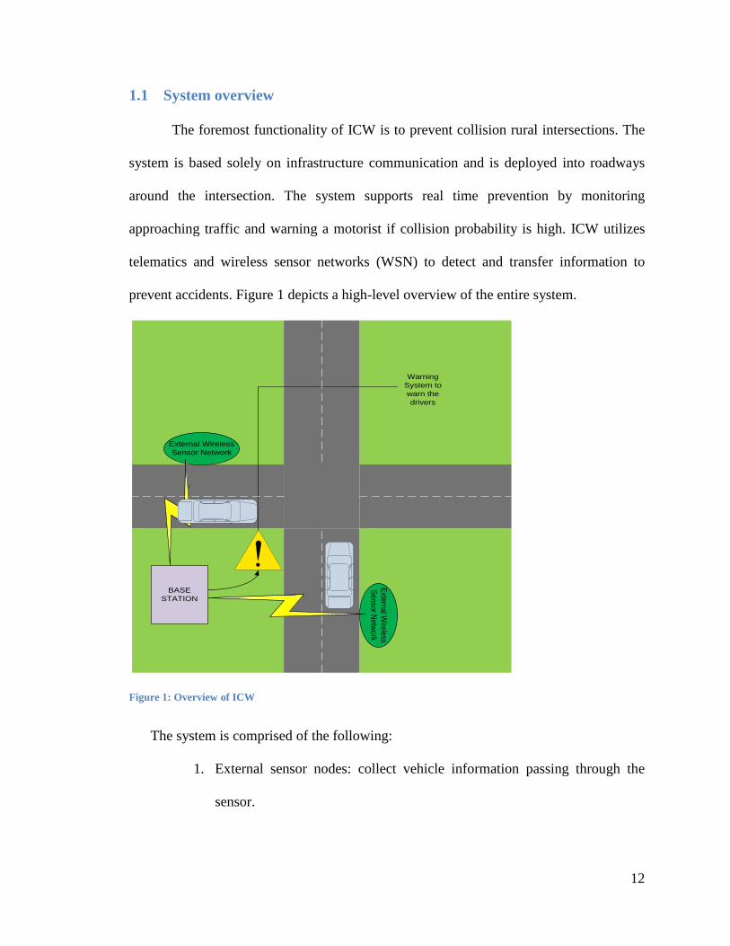
1.1 System overview
The foremost functionality of ICW is to prevent collision rural intersections. The
system is based solely on infrastructure communication and is deployed into roadways
around the intersection. The system supports real time prevention by monitoring
approaching traffic and warning a motorist if collision probability is high. ICW utilizes
telematics and wireless sensor networks (WSN) to detect and transfer information to
prevent accidents. Figure 1 depicts a high-level overview of the entire system.
Figure 1: Overview of ICW
The system is comprised of the following:
1. External sensor nodes: collect vehicle information passing through the
sensor.
External Wireless Sensor Network
External Wireless
Sensor Network
Warning System to warn the drivers
BASE STATION

13
2. Base Station (BS): located on the junction of each intersection to analyze
data; receives collected information from external sensor nodes wirelessly.
3. Warning system: embedded on both mainline and minor road junctions to
activate a warning signal after BS has analyzed data and determined the
possibility of a collision.
1.2 Organization
The balance of this report is organized as follows. Chapter 2 will discuss the
available technologies for intersection collision avoidance and their disadvantages.
Current research will be presented as well. Chapter 3 will discuss the presented
intersection collision avoidance. To provide a logical explanation of the algorithms used,
system requirements are listed. The chapter also lists the chosen system components and
gives logical analysis for each choice. Afterwards, a detailed hardware description is
presented. Finally, the chapter ends with the system wireless communication design.
Chapter 4 represents the processing aspect of the system. All the software algorithms that
are used are discussed and presented. Chapter 5 will present simulated test results that
was conducted in a lab sitting and provide appropriate discussion for each test.
14
2 Background
2.1 Background of intersection Traffic control devices
Intersection traffic control devices are comprised of signs, signals, roundabouts or
pavement markings that can be placed alongside the intersection. They are used to move
vehicles and pedestrians safely and efficiently, consequently preventing collisions by
providing the “right-of-way” principle assignment. The Federal Highway Administration
periodically publishes recommendations on how to setup specific control devices in its
manual on Uniform Traffic Control Devices (MUTCD) [6], thus ensuring safety by
standardizing operations. The most extensively used devices for current traffic control
include traffic signals, stop signs and roundabouts. These are explained in this section.
2.1.1 Traffic Signals
Traffic signals are used to assign right-of-way for drivers with the use of signal
lights (Red - Amber - Green). The universal standard for this three-light set is red on top,
amber in the middle, and green on the bottom. However, widely accepted road rules may
differ throughout the world, depending on how the traffic lights are interpreted. For
example, in most countries green means go and amber means prepare to stop, while red
means stop. Conversely, Canada and New Zealand consider amber red, which interpreted
as stop to their citizens.
Traffic signals are typically used at busy intersections to evenly distribute the time delay
between different directions at the intersection. The purpose is to ensure smoothness in
the traffic flow. Previously, the timing delay for light color change was fixed; however,
newer signals utilize vehicle detection for light color change.
15
2.1.2 Stop signs
In addition to traffic signals, stop signs are also used to control driver behavior.
Stop signs are usually installed at road junctions and instruct drivers to stop, check the
road and proceed if the road is clear. The standard stop sign has a specified size of 75 cm
(30 in) across opposite flat sides of the red octagonal field, with a 20 mm (¾ in) white
border [7]. Stop signs are mostly used for low to medium levels of traffic [8]. They are
usually best suited for rural highway intersections. If the traffic volume for a four-way
intersection is approximately equal in all directions, a four-way stop sign can also be
used.
2.1.3 Roundabouts
Roundabouts are another solution for intersection traffic. In the United States
these are often referred to as a “rotary” or “traffic circle”. A roundabout brings together
conflicting traffic streams by allowing vehicles to safely merge and traverse the
roundabout, and then exit in a desired direction. In essence, traffic enters a one-way
stream around a central island. There are many types of roundabouts and usually depends
on the intersection design. Roundabouts often provide a more safe type of traffic control
when compared to other methods. They are recognized for having fewer delays, increased
traffic circulation efficiency and enhanced community aesthetics.
2.1.4 Disadvantage and Limitation of Conventional Intersection Control Devices
2.1.4.1 Installation and Placement
Installing traffic control devices in unnecessary locations may lead to significant
traffic flow to the increase of unwanted delays in an intersection. This might not only
16
annoy drivers but would also increase fuel consumption. For example, a four way stop
sign might be justified when the traffic volume on all four sides is equal; however, if not,
unnecessary delays could occur. Moreover, the improper placement of a traffic control
device may decrease the efficiency of the system. A driver may see the signal too late to
safely react to the situation, which may lead to an increase in the number of accidents at
the intersection. One such example is placing the device too closely around the bend of a
sharp curve. Catastrophic results will occur when drivers fail to stop in time.
Sudden changes that could potentially happen along the intersection pose other safety
issues. For example, emergency vehicles assisting with a disastrous situation would lead
to an increase in traffic throughout the entire intersection. Conventional traffic control
devices are superseded by police officers attempting to manage traffic flow.
2.1.4.2 Safety
The primary goal of all traffic control devices is to maintain the safety of the drivers
advancing through the intersection. Conventional devices currently in use have
significant shortcomings that hinder due to physical and electrical infrastructure
requirements. This is especially true under certain conditions,
Traffic signal lights are one such example. When configuring a signal light an engineer
must be careful with the timing of the amber (yellow) light. If the illuminated time is too
short, drivers might have to slam on their brakes to avoid crossing the intersection when
the light turns red. This could cause an increase in real-end collisions. On the other hand,
if the time the amber (yellow) light is illuminated is too long, drivers might ignore it and
continue through the intersection, which might result in intersection collisions.
17
Stop signs can be just as dangerous. They are easily susceptible to vandalism or weather
conditions. If this occurs, a vehicle entering an intersection that is typically dangerous
won’t be warned to stop, thinking rather that it is safe to go through. This might result in
collision.
2.1.4.3 Cost
The cost of a traffic control lighting system depends on the complexity of the
intersection and the properties of the traffic using it. This is dependent not only on
installation, but maintenance, as well. While the cost of a traffic control has traditionally
been perceived as justified, in reality one traffic signal costs the range of $80,000 to
$100,000 for installation only. Often the perpetual costs, such as electrical power
consumption, are not considered [9].
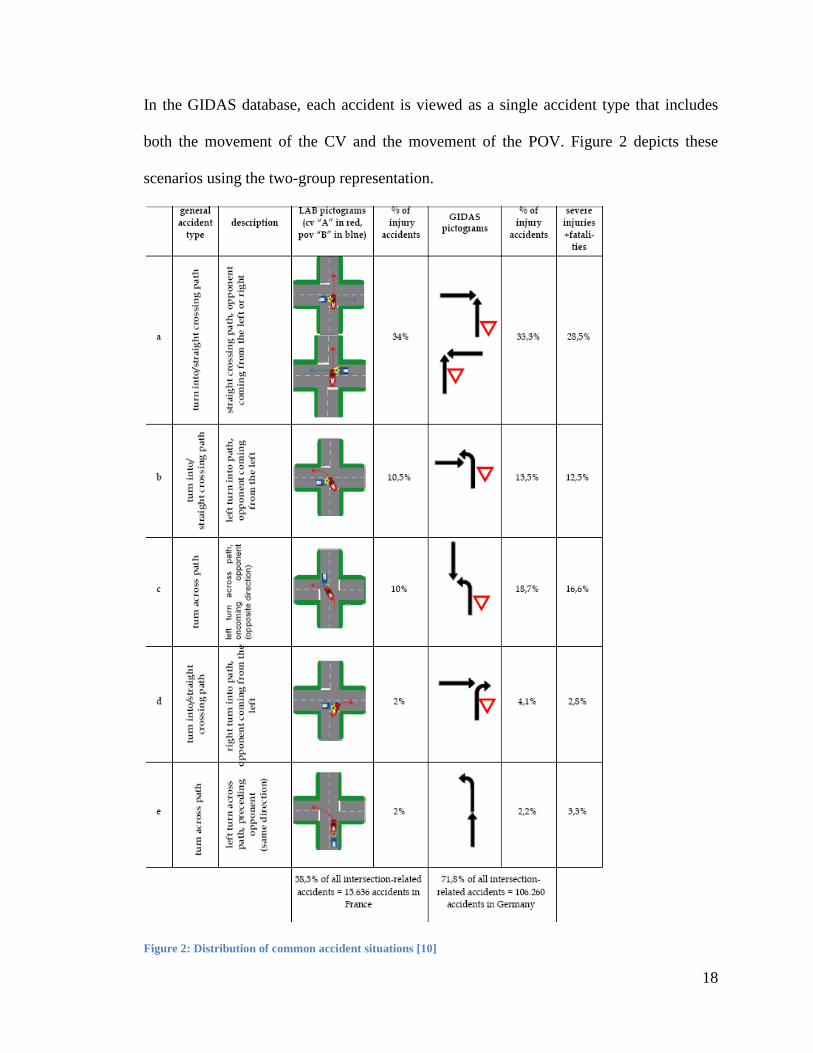
2.2 Causes of Intersection-Related Collision
As mentioned earlier, intersection-related collisions constitute the majority of
collisions. Consequently, knowing the source of collisions is of great importance.
According to the INTERSAFE project [10], five scenarios represent between
approximately 60% and 72% of injury accidents at intersections in France and Germany.
These are further defined as belonging to two accidents types, namely turn across path
and turn into/straight crossing path. Two groups, LAB and GIDAS provide the data for
the study. Data from the LAB database classifies an accident as follows:
• A vehicle (case vehicle, CV) pulls into an intersection after ignoring a stop
sign. This defines the situation.
• Another vehicle (principal other vehicle, POV) must compensate for the
vehicle suddenly cutting across his path.
18
In the GIDAS database, each accident is viewed as a single accident type that includes
both the movement of the CV and the movement of the POV. Figure 2 depicts these
scenarios using the two-group representation.
Figure 2: Distribution of common accident situations [10]
19
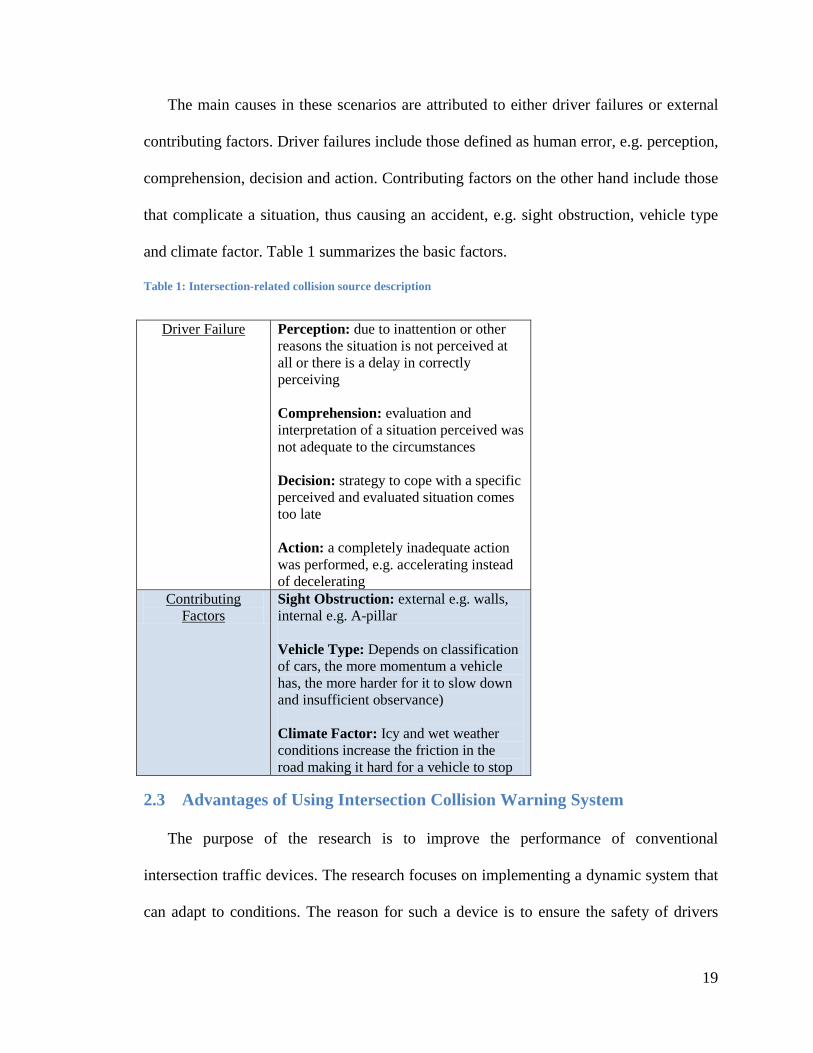
The main causes in these scenarios are attributed to either driver failures or external
contributing factors. Driver failures include those defined as human error, e.g. perception,
comprehension, decision and action. Contributing factors on the other hand include those
that complicate a situation, thus causing an accident, e.g. sight obstruction, vehicle type
and climate factor. Table 1 summarizes the basic factors.
Table 1: Intersection-related collision source description
Perception: due to inattention or other reasons the situation is not perceived at all or there is a delay in correctly perceiving
Driver Failure
Comprehension: evaluation and interpretation of a situation perceived was not adequate to the circumstances Decision: strategy to cope with a specific perceived and evaluated situation comes too late Action: a completely inadequate action was performed, e.g. accelerating instead of decelerating Sight Obstruction: external e.g. walls, internal e.g. A-pillar
Contributing Factors
Vehicle Type: Depends on classification of cars, the more momentum a vehicle has, the more harder for it to slow down and insufficient observance) Climate Factor: Icy and wet weather conditions increase the friction in the road making it hard for a vehicle to stop
2.3 Advantages of Using Intersection Collision Warning System
The purpose of the research is to improve the performance of conventional
intersection traffic devices. The research focuses on implementing a dynamic system that
can adapt to conditions. The reason for such a device is to ensure the safety of drivers
20
coming toward an intersection. The benefits of such a system can be summarized as
follows:
• Using a decentralized system that can be used in dense traffic
• Utilizing telematics for sensing and reporting
• Enabling drivers to be aware of their environment, even if line of sight is
not present
• Implementing a low cost device that can be adapted to any intersection
• Developing a collision warning system that captures driver attention
• Providing a system that is easily installed and maintained.
• Using a system that can be easily configured for other functions, such as
vehicle count, thus providing an input for traffic analysis systems
2.4 Literature Review
There has been increased interest from the United States (US) Department of
Transportation to develop and implement an efficient traffic control device. This has in
turn resulted in an increase in research focused on and defined as vehicle-to-vehicle
communication (v2v), vehicle to road communication (v2r) and road to road
communication (r2r). The v2v can be categorized into 3 classes based on the technology
used: 1) radar based [11][12], 2) camera based [13][14] and 3) radio based system [15].
Radar-based and camera-based technologies are used to avert collisions in the same lane
as a result of line of sight limitation. Radio-based technologies have a broader use for
collisions independent of either line of sight or passing lanes.
V2r applications focus primarily on an intersection warning system, whether it is
embedded inside the vehicle or externally. Most v2r use DGPS technology to support a
21
base station installed at a junction, thus facilitating required vehicle information to the
prediction [16][17]. Alternative implementations are possible. For example in [18] a
unique RFID is embedded in each vehicle for differentiation purposes. The system makes
use of WSN in the road to supply the BS with information necessary for prediction.
R2r communication, on the other hand, is totally independent of the vehicles. Sensing
functionality is the focus of such a system. The control device has the ability to fetch
information about a vehicle in real-time scenario. A variety of such approaches have been
made. One uses WSN technologies that adopt magnetic sensors [19]. Another uses a
radar as a sensing functionality [20]. Vision methods can also be employed [21].
Three important intersection collision avoidance programs are currently being
conducted in the US and are funded by Intelligent Transportation System (ITS). These
are lead by University of California (UC Berkeley), the University of Minnesota (UMN)
and Virginia Polytechnic Institute/Virginia Tech Transportation Institute (VTTI). The UC
Berkeley program is known as the Partners for Advanced Transit and Highways (PATH),
and it supports about 65 projects related to transportation safety research. One of their
innovative research endeavors focuses on a warning system placed at a signaled
intersection to warn drivers from a possible collision. This system employs a group of
loop detection sensors and radars that communicate wirelessly with the traffic light
system to warn drivers [22]. UMN research is similar to the PATH project. Intelligent
Vehicles Laboratory and Policy & Planning for ITS are two of their foremost projects.
The UMN Intelligent Vehicles lab is the first to focus on developing and testing
innovative technologies that reduce driver error by integrating sensor networks, vehicle
control systems, navigation systems, and specially designed human interface components.
22
The Planning for ITS program is designed to equip transportation and infrastructure
professionals with the technological tools to address congestion and other system
challenges in the coming years. The focus is on collisions that occur at an unsignalized
intersection [23]. VTTI projects are equally as important. They focus on collisions due to
traffic signal and stop sign violations. VTTI is the largest research center at the
university, containing nine center groups dealing with different types of transportation
issues.
One drawback to the aforementioned research projects is that all are vehicle
dependent, i.e. the vehicle is equipped with either sensors or a warning system. The
shortcoming of this approach is that the system would require equipment be installed in
each vehicle. While not expensive, the implementation would be lengthy. Some
researchers have therefore abandoned the vehicle equipment approach [25][26]. Instead,
their systems are now mainly comprised of wireless road sensors that transmit traffic
flow information to a base station. The BS will generate a predictive analysis calculating
whether a collision might take place, and then send a warning signal from an embedded
mechanism in the road if there is a possibility of an accident. Another drawback to PATH
and VTTI projects is their message routing implementation. For example, PATH employs
Time Division Multiple Access, where as VTTI employs wireless mesh networks. Both
technologies achieve high message latency that is not tolerable for intersection collision
avoidance systems.
In addition to intersection collision avoidance research, a commercially available
product has been developed by Sensys Network Inc. IT is comprised of repeaters, access
points and wireless sensors, and in addition to vehicle count and stop bar detection, it can
23
predict a vehicle’s trajectory [27]. The product uses a Time Division Multiple Access
(TDMA) technique to enable sensor nodes to communicate with a base station. The major
drawback for such a product is its latency time, as each node must wait approximately
125 ms to communicate with the base station if its time slot has already passed. This is
unacceptable for an intersection warning system, as it should be time-latency sensitive;
the less the delay, the better system will operate.
24
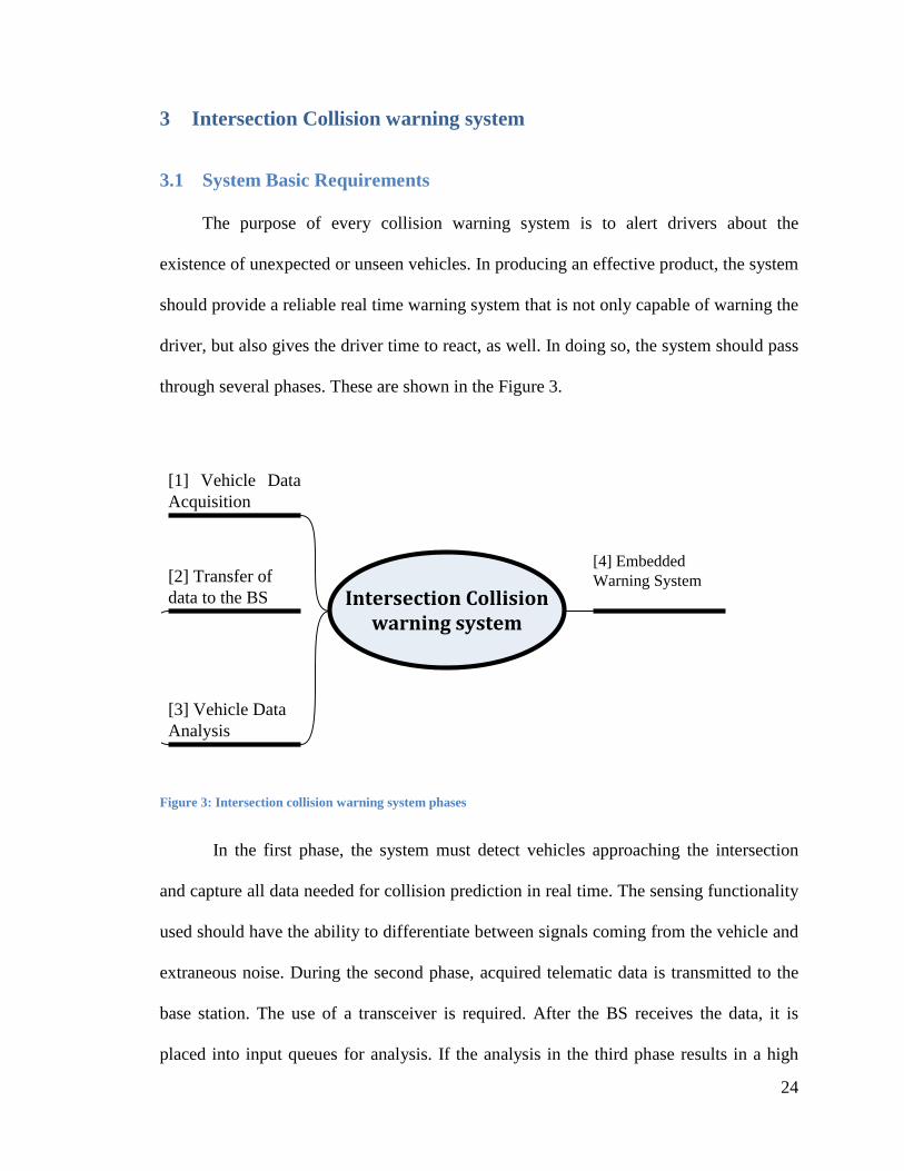
3 Intersection Collision warning system
3.1 System Basic Requirements
The purpose of every collision warning system is to alert drivers about the
existence of unexpected or unseen vehicles. In producing an effective product, the system
should provide a reliable real time warning system that is not only capable of warning the
driver, but also gives the driver time to react, as well. In doing so, the system should pass
through several phases. These are shown in the Figure 3.
Figure 3: Intersection collision warning system phases
In the first phase, the system must detect vehicles approaching the intersection
and capture all data needed for collision prediction in real time. The sensing functionality
used should have the ability to differentiate between signals coming from the vehicle and
extraneous noise. During the second phase, acquired telematic data is transmitted to the
base station. The use of a transceiver is required. After the BS receives the data, it is
placed into input queues for analysis. If the analysis in the third phase results in a high
Intersection Collision warning system
[4] Embedded Warning System[2] Transfer of
data to the BS
[1] Vehicle Data Acquisition
[3] Vehicle Data Analysis
25
probability of collision, a warning system is activated to alert drivers of possible
collision.
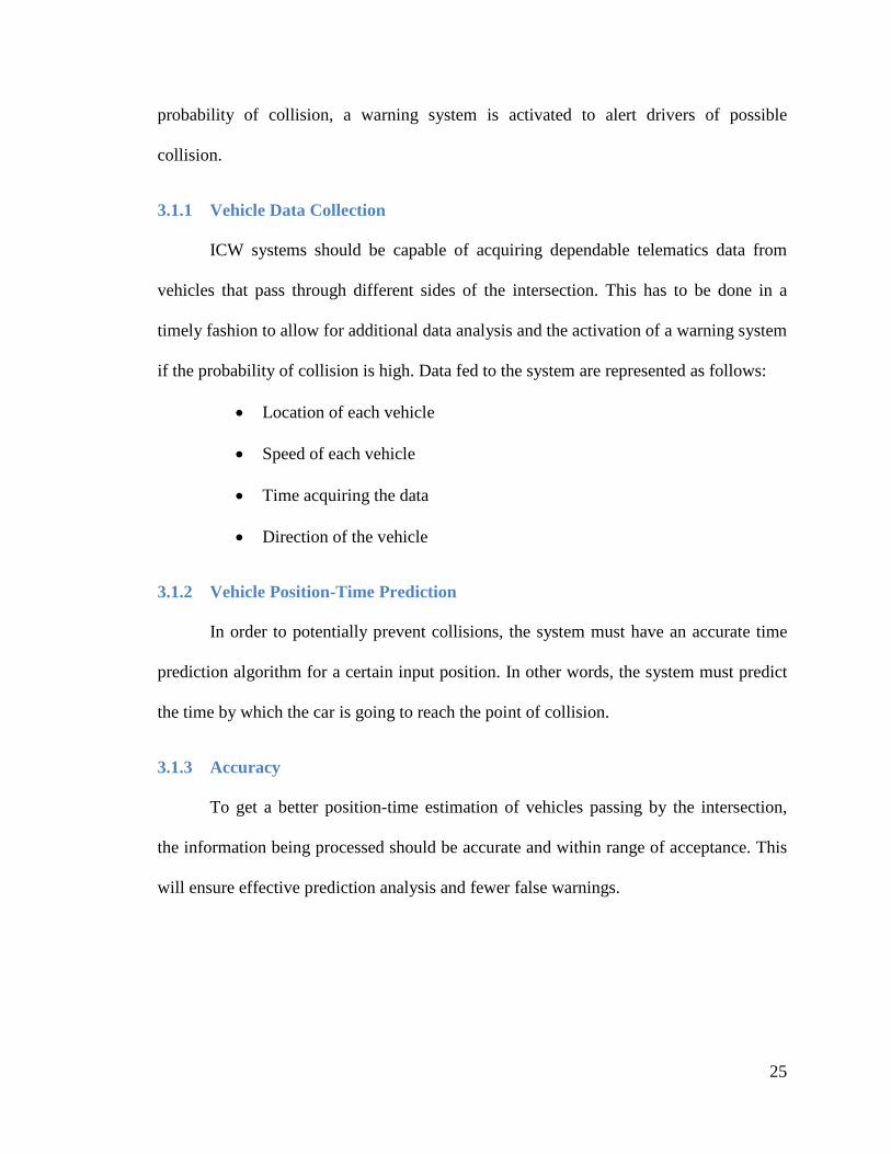
3.1.1 Vehicle Data Collection
ICW systems should be capable of acquiring dependable telematics data from
vehicles that pass through different sides of the intersection. This has to be done in a
timely fashion to allow for additional data analysis and the activation of a warning system
if the probability of collision is high. Data fed to the system are represented as follows:
• Location of each vehicle
• Speed of each vehicle
• Time acquiring the data
• Direction of the vehicle
3.1.2 Vehicle Position-Time Prediction
In order to potentially prevent collisions, the system must have an accurate time
prediction algorithm for a certain input position. In other words, the system must predict
the time by which the car is going to reach the point of collision.
3.1.3 Accuracy
To get a better position-time estimation of vehicles passing by the intersection,
the information being processed should be accurate and within range of acceptance. This
will ensure effective prediction analysis and fewer false warnings.
26
3.1.4 Coverage Area
Coverage areas can be represented by either distance or time. The coverage of the
system, or in other words the range by which the system should start collecting data, must
take into account important variables. These are represented as follows:
• Normal deceleration period while reaching the intersection
• Deceleration period needed to come to full stop (pressing hard on the
brakes)
• Reaction period of the driver
• Processing period of the system
3.1.5 Arbitrary Approaches
Vehicles usually approach an intersection arbitrarily. Consequently, random
approaches should not affect the system. As soon as a vehicle advances through the
intersection, the system should be able to detect its presence and send the information
back for analysis.
3.1.6 Real time
Safety is the focus of the system; therefore, it is essential to obtain data in a timely
manner. The moment a vehicle reaches the coverage area, data has to be collected and
sent to the BS immediately for analysis. This will ensure the driver has time to react
before the collision occurs.

27
3.1.7 Cost Effective
The purpose of the ICW is to implement a system that is not only effective and
efficient, but also one that is affordable in both prediction time and cost. If a system is to
be implemented at the intersection, certain costs should be considered:
• System components
• Installation
• Distribution
• Maintenance and calibration
• Development
3.2 System Component
3.2.1 Sensors
ICW should be able detect the presence of a moving vehicle through the
intersection. In doing so, the system requires a sensing functionality that is able to detect
the presence of a vehicle and convert its location to traffic parameters. This functionality
must have the ability to fetch all data needed in this phase.
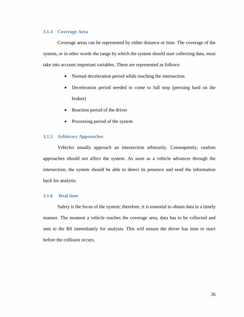
In determining the best product for the system, a consideration of a comparison of
different sensors made by the Vehicle Detector Clearing House Corporation [29] was
conducted. Figure 4 characterizes sensor technologies and their capabilities. Output data
for each available sensor along with its lane coverage, communication bandwidth and the
purchase cost is listed.
28
Figure 4: Sensor comparison [29]
Picking a suitable sensor for the system should be dependent upon basic
requirements aforementioned. Classification capability is not be of huge importance, as
this feature is not addressed in this report.

29
Lower priced sensors within our expenditure limits provide only inductive loops,
magnetometer and magnetic sensors. Others that are higher priced provide additional
noise filter that is beneficial for vehicle detection and tracking. A major disadvantage,
however, is poor performance during inclement weather conditions. Inductive loops are
not reliable. On the other hand, wire loops are subject to stress of traffic and temperature.
A study by the University of Berkeley demonstrates the accuracy of magnetic sensors in
detecting, classifying and calculating the speed of the vehicles [30]. It shows a vehicle
detection rate of100 percent and more than 90 percent for speed calculation.
Consequently, magnetic sensors are the logical choice for the system. In addition to their
high accuracy rate, these sensors are insensitive to inclement weather conditions, e.g.
snow, rain and fog, and are easily deployed and maintained.
An important consideration to be noted is the addition of the power efficiency issue to the
basic system requirement. This is highly important due to the fact that magnetic sensors
are to be deployed under the road where a power source is not provided. An expected
long life and minimum cost maintenance should be expected, as customer satisfaction
will be directly related. A study on energy consumption appears in later in this chapter.
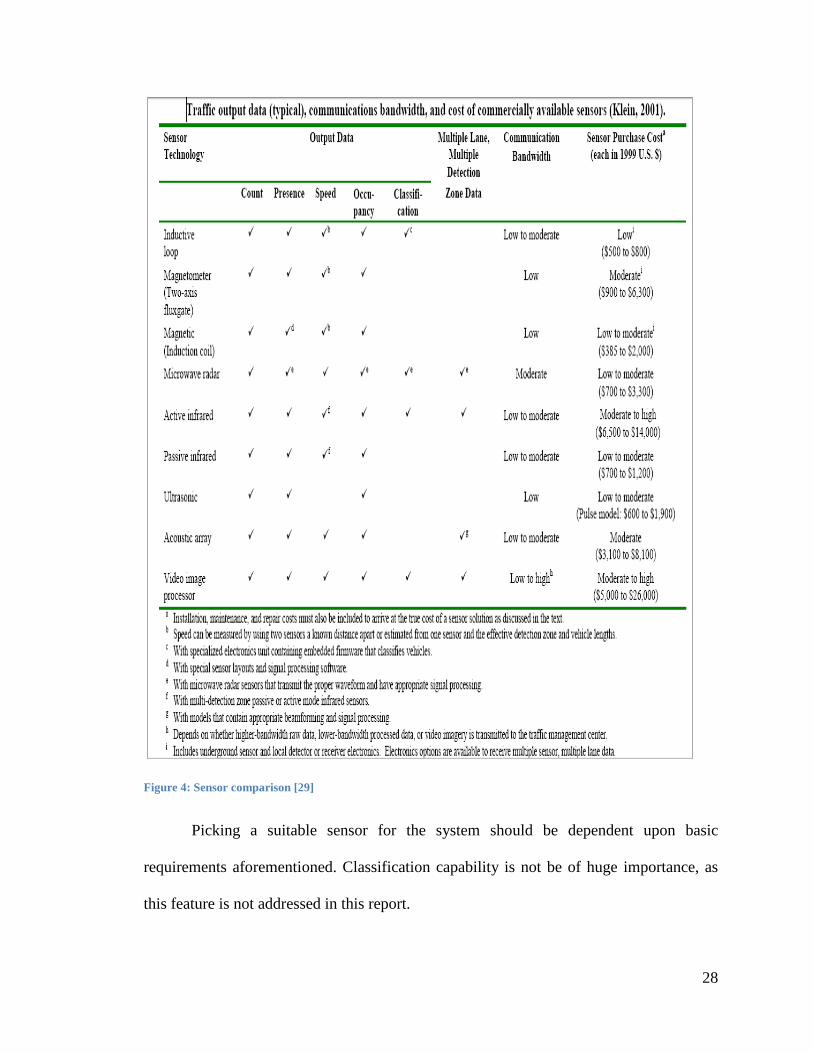
3.2.1.1 Magnetic Sensor technology
Magnetic sensors are passive devices that detect changes in the earth’s magnetic field.
After detection they convert a highly localized disruption to a differential voltage output.
When a vehicle passes by a sensor, the field alteration caused by different parts of the
vehicle is recorded. Figure 5 shows changes in the output of the magnetic sensor when a
vehicle travels over it.
30
Figure 5: Magnetic anomaly in the Earth’s magnetic field induced by magnetic dipoles in a ferrous metal vehicle
[29]
3.2.1.2 Honeywell HMC1021Z
Honeywell is widely recognized as a leading manufacturer of magnetic sensors; the
company is well known for their reliable products and excellence. The HMC1021Z
sensor has been chosen for this research from their wide variety of product selection. The
sensor is a one-axis surface mount that utilizes Honeywell’s Anisotropic Magneto
resistive technology. It is cost effective and was designed for low field magnetic sensing
from tens of micro-gauss to six gauss [31].
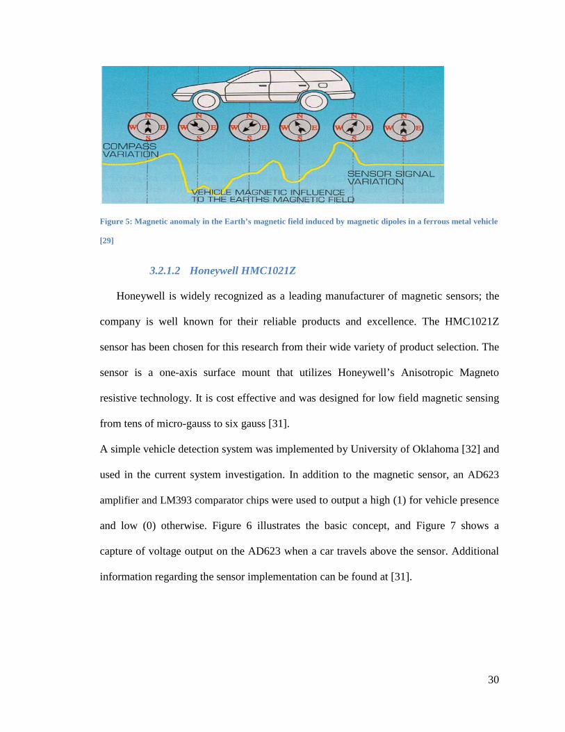
A simple vehicle detection system was implemented by University of Oklahoma [32] and
used in the current system investigation. In addition to the magnetic sensor, an AD623
amplifier and LM393 comparator chips were used to output a high (1) for vehicle presence
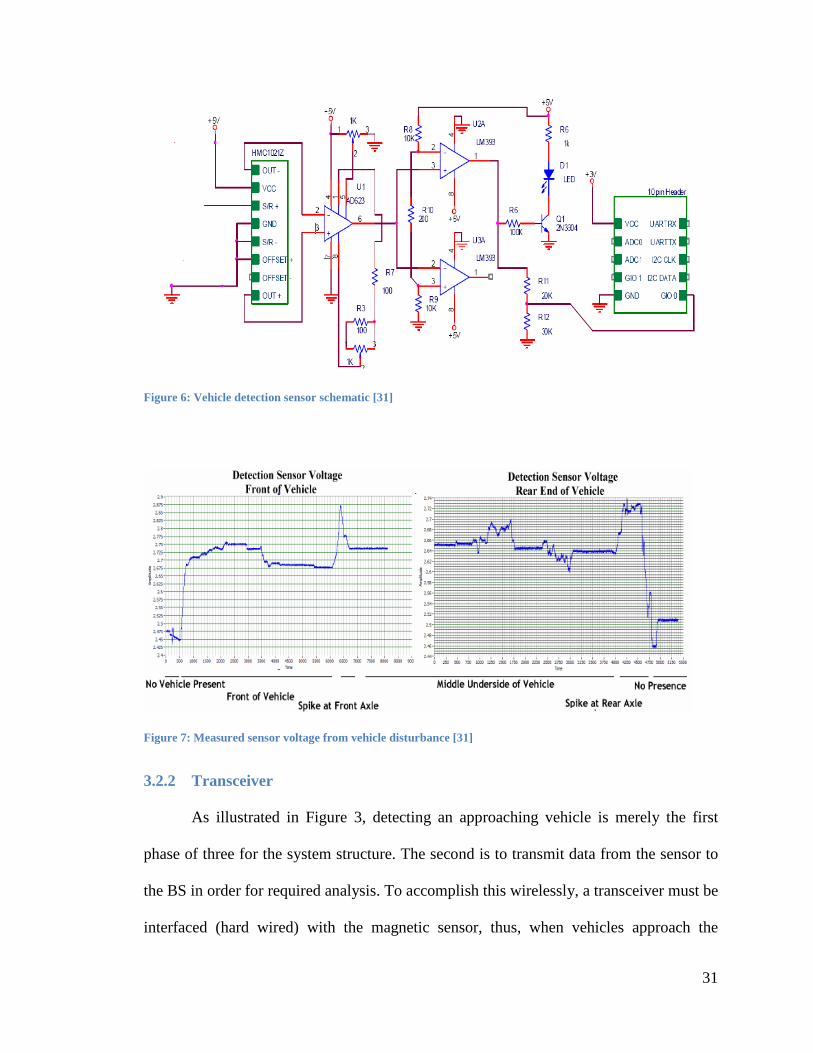
and low (0) otherwise. Figure 6 illustrates the basic concept, and Figure 7 shows a
capture of voltage output on the AD623 when a car travels above the sensor. Additional
information regarding the sensor implementation can be found at [31].
31
Figure 6: Vehicle detection sensor schematic [31]
Figure 7: Measured sensor voltage from vehicle disturbance [31]
3.2.2 Transceiver
As illustrated in Figure 3, detecting an approaching vehicle is merely the first
phase of three for the system structure. The second is to transmit data from the sensor to
the BS in order for required analysis. To accomplish this wirelessly, a transceiver must be
interfaced (hard wired) with the magnetic sensor, thus, when vehicles approach the

32
intersection, the sensor will detect changes in the earth’s magnetic field and the
transceiver linked to the sensor should immediately transfer the telematic data wirelessly
to the BS. Details about the system structure are discussed later in this chapter.
The choice for an ICW transceiver should be based on the consideration of
imperative parameters; most important are unit range, power consumption, interface,
temperature and price. While the detection signal and time synchronization parameters
will be sent in the wireless domain; the throughput does not constitute high importance
due to the small size of the data packet. Table 2 summarizes the capabilities of popular
transceivers considered for the system. As shown, only the Radiotronix Wi.232DTS
fulfilled all requirements. The remainder are either too costly or require an unnecessarily
high output power.
Table 2: Candidate transceivers
Radiotronix
Wi.232DTS [33]
AeroComm,
AC4790-
200[34]
Z-Accel 2.4 GHz
ZigBee [35]
UHF902-928 [36]
Price (a piece) 20$ 63.85$ 99$ 55$
Frequency 902 - 928 MHz 902 - 928 MHz 2400 - 2483.5
MHz
902 - 928 MHz
Range 1 mile Up to 4 miles
1 mile
1.5 miles
Output Power Up to 25 mW Up to 200 mW
27 mW (lowest)
Up to 1 W
Needs Antenna Yes No
Yes
Yes
Programmabili
ty
Yes Yes Yes Yes
Interface SCI SCI
SCI
SCI
Throughput Up to 152.32 76.8 kbps 250 Kbps 57.6 Kbps
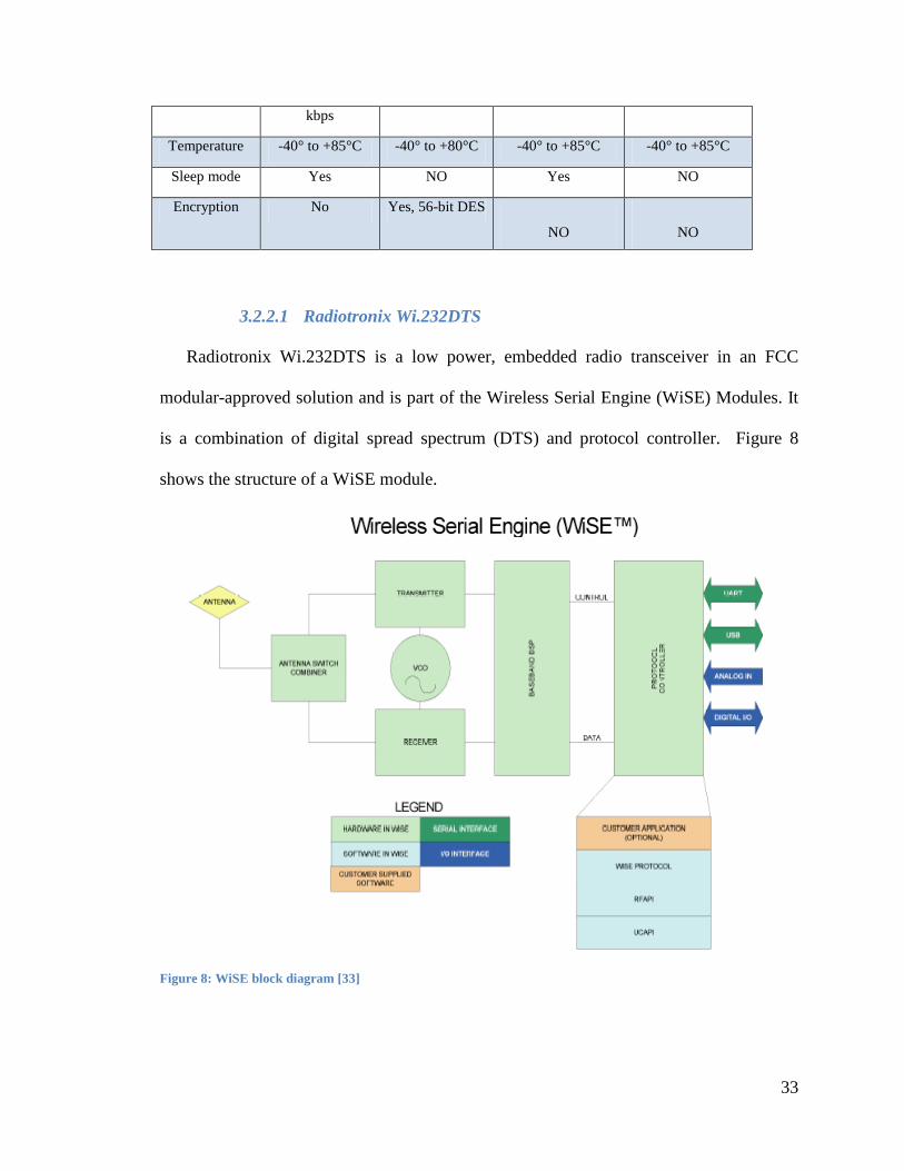
33
kbps
Temperature -40° to +85°C -40° to +80°C -40° to +85°C -40° to +85°C
Sleep mode Yes NO Yes NO
Encryption No Yes, 56-bit DES
NO
NO
3.2.2.1 Radiotronix Wi.232DTS
Radiotronix Wi.232DTS is a low power, embedded radio transceiver in an FCC
modular-approved solution and is part of the Wireless Serial Engine (WiSE) Modules. It
is a combination of digital spread spectrum (DTS) and protocol controller. Figure 8
shows the structure of a WiSE module.
Figure 8: WiSE block diagram [33]

34
One of outstanding features of Wi.232DTS is its support for the universal
asynchronous receiver/transmitter (UART) protocols, which ensures ease of access to
data module registers. Wi.232DTS supports four power modes—DTS low/ high and Low
power low/high; this feature gives the system the necessary feasibility to select optimal
power options. Sleep mode is an important feature, as well; it is essential for power
control, which is highlighted later in this report. Basic module features are listed in Table
3 below.
Table 3: Feature summary for WI.232DTS module
Feature Description Interface True UART to antenna solution
Error checking 16-bit CRC error checking
Data rate 100kbit/ sec maximum effective RF data rate
# of channels 32 channels in DTS mode, 84 channels in LP mode, North American Version
Size Small size- .8” x .935” x .08”
Low Power
Options
Low power Standby and Sleep modes
Protocol Layers PHY and MAC layer protocol built in
MAC CSMA medium access control
Network Group 0-127 Networks
Network Mode Normal and Slave
Link Budget 115dB link budget in DTS mode
Power modes 4 modes allow user to optimize power/ range
Configuration Command mode for volatile and non-volatile configuration
3.2.3 Microcontroller
A major component requirement for the system is a processing functionality capable
of performing data analysis in a reliable, energy-efficient and real-time manner. Essential
functionalities for the processer include the ability to:
• Transfer data from the magnetic sensor to the transceiver and eventually to BS

35
• Perform time synchronization for better collision detection
• Perform collision detection logic when data is available from all sensors
The system does not require a high computational processor to perform the functions
listed above. Hence, a low-cost versatile microcontroller is suitable for the project, as it
performs the all requirements in an efficient and effective way. Component features
necessary for the system are listed in the following table.
Table 4: Expected microcontroller features
Issue Feature
Energy Efficiency Low power consumption
Sleep mode functionality
Sleep mode Interrupt driven
Sensor Interface Digital I/O inputs
Transceiver Interface UART serial communication
Speed Fast sleep wake up
Temperature Change Reliable Oscillator
Microchip is a well-known manufacturer of Programmable Intelligent Computer
(PIC) microcontrollers [37]. The company produces a wide variety of PIC technologies,
ranging from 12- to 16-bit flash microcontrollers. The PIC is a powerful, completely
featured processor with internal RAM, EEROM FLASH memory and a broad range of
peripherals. The microcontrollers are small and can easily be programmed to accomplish
a number of tasks. High-level programming, e.g. C language, can be accomplished, as
can lower level, such as Basic or Assembly. The Microchip microcontroller comes with a
36
free MPLAB integrated design environment, which is comprised of an assembler, linker,
integrated C, software simulator, and debugger.
PIC24FJ128GA010 was chosen from the broad range of PIC products because of its
higher computational performance. This model can support up to a 16 MIPS (million
instructions per second) Operation at 32 Mhz, thus ensuring superior system utilization.
The PIC uses a 16-bit data and 24-bit address path to register access. In addition to these
core features, it has a built in 8 Mhz internal oscillator able to amplify to 32 Mhz using its
Phase Lock Loop (PLL) frequency multiplier functionality. For low-power use, a 31 Khz
oscillator is integrated in the PIC. This is extremely important in applications required to
maintain minimal power usage. Usability of external oscillators is feasible in the
PIC24FJ128GA010, as it utilizes two crystal and two external clock modes. Serial
communication can be accomplished using the fully equipped, two independent
Universal asynchronous receiver/transmitter (UART) and two independent Serial
Peripheral Interface (SPI) modules in the PIC. This microcontroller supports parallel
communication, as well. Likewise, it supports a Parallel Master Port (PMP) module used
to communicate with devices that support parallel communication. Additionally, the PIC
implements a full-featured clock and calendar with alarm functions in its hardware. This
particular module is optimized for low-power operation. It uses an integrated, low-power
oscillator for clock synchronization, and sleep mode with fast wake up time is also
applicable. The unit consumes current as low as 120µA while in sleep mode and can
increase to120µs to wake up.
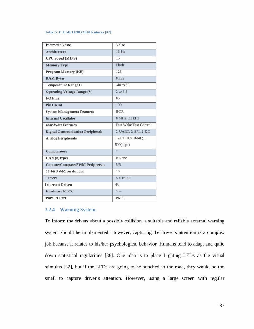
A summary of these important features are listed in the table below.
37
Table 5: PIC24FJ128GA010 features [37]
Parameter Name Value
Architecture 16-bit
CPU Speed (MIPS) 16
Memory Type Flash
Program Memory (KB) 128
RAM Bytes 8,192
Temperature Range C -40 to 85
Operating Voltage Range (V) 2 to 3.6
I/O Pins 85
Pin Count 100
System Management Features BOR
Internal Oscillator 8 MHz, 32 kHz
nanoWatt Features Fast Wake/Fast Control
Digital Communication Peripherals 2-UART, 2-SPI, 2-I2C
Analog Peripherals 1-A/D 16x10-bit @
500(ksps)
Comparators 2
CAN (#, type) 0 None
Capture/Compare/PWM Peripherals 5/5
16-bit PWM resolutions 16
Timers 5 x 16-bit
Interrupt Driven 43
Hardware RTCC Yes
Parallel Port PMP
3.2.4 Warning System
To inform the drivers about a possible collision, a suitable and reliable external warning
system should be implemented. However, capturing the driver’s attention is a complex
job because it relates to his/her psychological behavior. Humans tend to adapt and quite
down statistical regularities [38]. One idea is to place Lighting LEDs as the visual
stimulus [32], but if the LEDs are going to be attached to the road, they would be too
small to capture driver’s attention. However, using a large screen with regular
38
background color change deployed beside the road would be enough to get driver’s
attention.
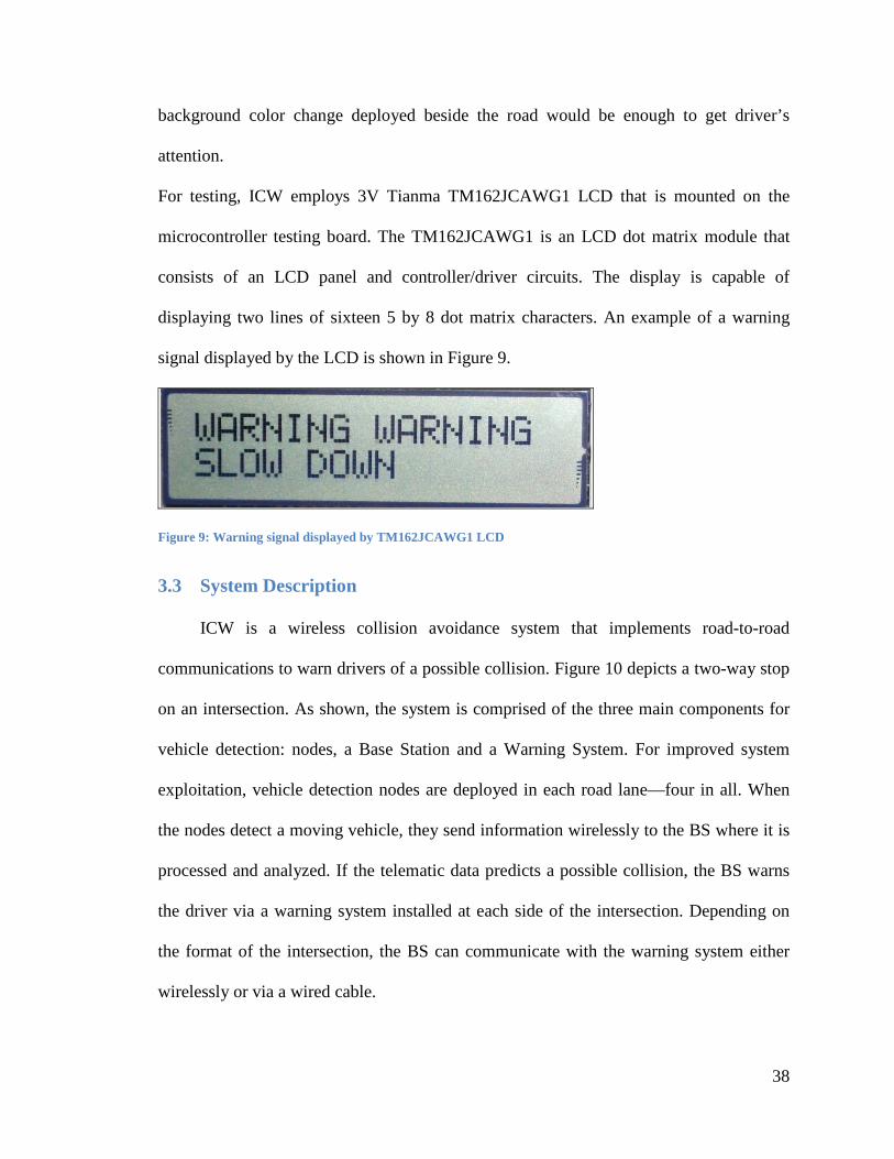
For testing, ICW employs 3V Tianma TM162JCAWG1 LCD that is mounted on the
microcontroller testing board. The TM162JCAWG1 is an LCD dot matrix module that
consists of an LCD panel and controller/driver circuits. The display is capable of
displaying two lines of sixteen 5 by 8 dot matrix characters. An example of a warning
signal displayed by the LCD is shown in Figure 9.
Figure 9: Warning signal displayed by TM162JCAWG1 LCD
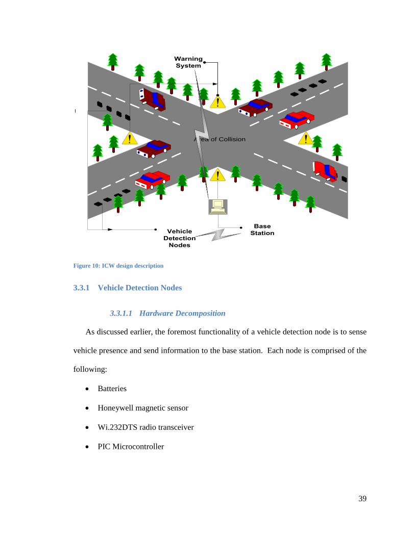
3.3 System Description
ICW is a wireless collision avoidance system that implements road-to-road
communications to warn drivers of a possible collision. Figure 10 depicts a two-way stop
on an intersection. As shown, the system is comprised of the three main components for
vehicle detection: nodes, a Base Station and a Warning System. For improved system
exploitation, vehicle detection nodes are deployed in each road lane—four in all. When
the nodes detect a moving vehicle, they send information wirelessly to the BS where it is
processed and analyzed. If the telematic data predicts a possible collision, the BS warns
the driver via a warning system installed at each side of the intersection. Depending on
the format of the intersection, the BS can communicate with the warning system either
wirelessly or via a wired cable.
39
Figure 10: ICW design description
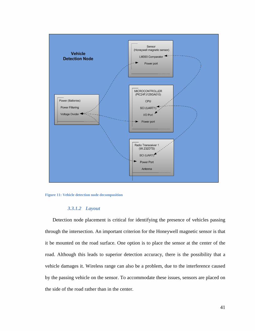
3.3.1 Vehicle Detection Nodes
3.3.1.1 Hardware Decomposition
As discussed earlier, the foremost functionality of a vehicle detection node is to sense
vehicle presence and send information to the base station. Each node is comprised of the
following:
• Batteries
• Honeywell magnetic sensor
• Wi.232DTS radio transceiver
• PIC Microcontroller
Area of Collision
Vehicle Detection
Nodes
Base Station
Warning System

40
Because nodes are deployed roadside where no power source is present, batteries
offer a simple solution. A voltage divider is added to the circuit to supply other
components with power.
In short, when a vehicle passes through the intersection, the magnetic sensor detects
fluctuation in the earth’s magnetic field. The analog signal is transformed to a digital via
a LM393 comparator embedded in the sensor design. The signal is then passed to the
microcontroller through one of the I/O ports. Afterwards, the CPU customizes the data
and sends it through the Serial Communication Interface (SCI) so it can be sent
wirelessly by the radio transceiver. SCI uses UART protocol as its serial transmission
protocol. Figure 11 shows the node’s hardware decomposition.
41
Figure 11: Vehicle detection node decomposition
3.3.1.2 Layout
Detection node placement is critical for identifying the presence of vehicles passing
through the intersection. An important criterion for the Honeywell magnetic sensor is that
it be mounted on the road surface. One option is to place the sensor at the center of the
road. Although this leads to superior detection accuracy, there is the possibility that a
vehicle damages it. Wireless range can also be a problem, due to the interference caused
by the passing vehicle on the sensor. To accommodate these issues, sensors are placed on
the side of the road rather than in the center.

42
The distance between detection nodes and the intersection is also critical. The system
must ensure that the warning system on the LCD is promptly displaced to warn the
drivers in time for them to respond. However, determining the appropriate warning
distance for the driver is foremost. Accordingly, a two dimensional motion model is
considered:
𝐷𝐷𝑆𝑆𝑆𝑆𝑆𝑆𝑆𝑆 = 𝑣𝑣𝑣𝑣2
2𝑎𝑎+ (𝑆𝑆𝑑𝑑𝑑𝑑𝑣𝑣𝑣𝑣𝑑𝑑𝑑𝑑 + 𝑆𝑆𝑚𝑚𝑎𝑎𝑚𝑚 ℎ𝑣𝑣𝑖𝑖𝑑𝑑 + 𝑆𝑆𝑆𝑆𝑑𝑑𝑆𝑆𝑚𝑚𝑑𝑑𝑝𝑝𝑝𝑝𝑣𝑣𝑖𝑖𝑝𝑝 + 𝑆𝑆𝑤𝑤𝑎𝑎𝑣𝑣𝑆𝑆 ) ∗ 𝑣𝑣𝑣𝑣
Where
• 𝑆𝑆𝑑𝑑𝑑𝑑𝑣𝑣𝑣𝑣𝑑𝑑𝑑𝑑 driver brake response time
• 𝑆𝑆𝑚𝑚𝑎𝑎𝑚𝑚 ℎ𝑣𝑣𝑖𝑖𝑑𝑑 braking system in addition to the warning system response time
• 𝑆𝑆𝑆𝑆𝑑𝑑𝑆𝑆𝑚𝑚𝑑𝑑𝑝𝑝𝑝𝑝𝑣𝑣𝑖𝑖𝑝𝑝 microcontroller Collision prediction processing time
• 𝑆𝑆𝑤𝑤𝑎𝑎𝑣𝑣𝑆𝑆 Maximum time the system has to wait to get information from the
other sensor group to perform collision prediction.
• 𝑣𝑣𝑣𝑣 initial velocity of the vehicle
• 𝑎𝑎 deceleration of the vehicle
As previously discussed in chapter 1, there are many sources for accidents in the
intersection. Consequently, to determine the values of the above parameters is considered
a real challenge. However, INTERSAFE project [10] has come up with reasonable values
that are based on accident analysis. The values are summarized in Table 6

43
Table 6: Stopping distance value range [10]
Min Max Average
𝒕𝒕𝒅𝒅𝒅𝒅𝒅𝒅𝒅𝒅𝒅𝒅𝒅𝒅 0.8 sec 2 sec 0.95 sec
𝒕𝒕𝒎𝒎𝒎𝒎𝒎𝒎𝒎𝒎𝒅𝒅𝒎𝒎𝒅𝒅 0.3 sec 0.5 sec 0.4 sec
𝒎𝒎 0.31 g = 3.038
𝑚𝑚/𝑝𝑝2
0.7 g = 6.86 𝑚𝑚/𝑝𝑝2 4.9490 𝑚𝑚/𝑝𝑝2
𝑆𝑆𝑆𝑆𝑑𝑑𝑆𝑆𝑚𝑚𝑑𝑑𝑝𝑝𝑝𝑝𝑣𝑣𝑖𝑖𝑝𝑝 is absent from the table above because of its relation to the microcontroller
processing power and the algorithm complexity. Therefore, microcontroller and
algorithms have differences in their timing processing speeds.
In the worst-case scenario, the system must use the maximum values stated above.
However, this renders the system vulnerable to inaccurate collision detection, due to the
fact that a driver will pass the sensors before the start of a deceleration phase. This might
result in predication bias. The deceleration phase is defined by the time a driver starts
decelerating. Hence, a suitable approach would be to take the average of the parameters
in Table 6. Considering this, we can assume the following:
• Speed limit as an initial velocity of 40 mph with 10 mph added to obtain a design
speed.
• 𝑆𝑆𝑆𝑆𝑑𝑑𝑆𝑆𝑚𝑚𝑑𝑑𝑝𝑝𝑝𝑝𝑣𝑣𝑖𝑖𝑝𝑝 value of 0.158 seconds to process data [32].
• 𝑆𝑆𝑤𝑤𝑎𝑎𝑣𝑣𝑆𝑆 value of 1 sec is assumed as a maximum waiting time.
The above equation would lead to an approximate warning distance of 105 meters.
Consequently, the last deployed detection node should be placed 85 meters far from the
intersection.
44
To calculate the total distance between the first sensor and the intersection, the system
must consider the spacing of the detection nodes. Two important criterions regarding
nodes spacing should be considered:
• not too small: to give chance for speed calculation to take place
• not too big: to keep the detection nodes within an acceptable intersection range
The most suitable approximation is to use a shade over a car length as the separation
distance. The average length of a car is about 4 meters [39]. For worst case scenarios 5
meters is used instead. With 4 detection nodes mounted on the road, the total distance
between the first deployed detection node and the intersection end is 5 ∗ 4 + 105 =125
meters.
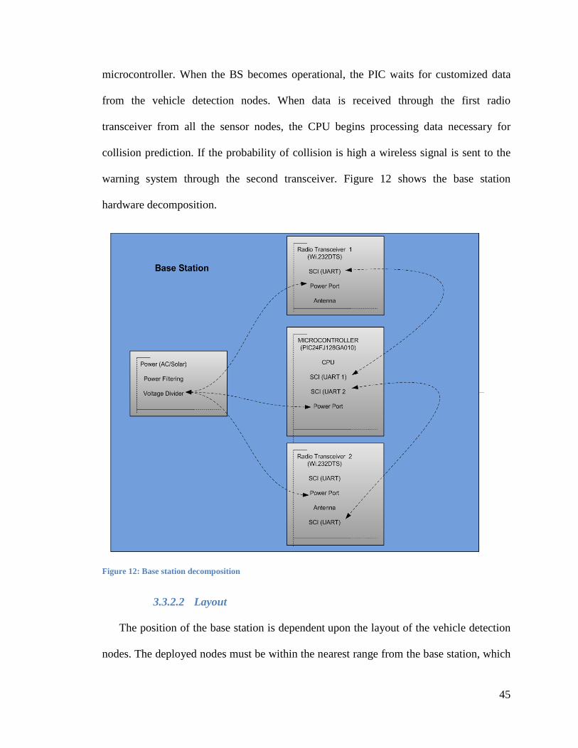
3.3.2 Base Station
3.3.2.1 Hardware Decomposition
The base station processes data received from the vehicle detection nodes and is
comprised of the following components:
• Batteries
• Two Wi.232DTS radio transceiver (each supports different radio channel)
• PIC Microcontroller
It is important to note that the BS supports two Wi.232DTS transceivers. Transceiver 1 is
used to communicate with the detection node, while Transceiver 2 is used to
communicate with the warning system. Although both transceivers are the same model,
they operate on different channels.
Either AC or solar power can provide power for the node. As in the detection
node, SCI (UART) is the communication interface between the transceivers and the
45
microcontroller. When the BS becomes operational, the PIC waits for customized data
from the vehicle detection nodes. When data is received through the first radio
transceiver from all the sensor nodes, the CPU begins processing data necessary for
collision prediction. If the probability of collision is high a wireless signal is sent to the
warning system through the second transceiver. Figure 12 shows the base station
hardware decomposition.
Figure 12: Base station decomposition
3.3.2.2 Layout
The position of the base station is dependent upon the layout of the vehicle detection
nodes. The deployed nodes must be within the nearest range from the base station, which
46
is typically best if cornered at the side of the intersection. An important consideration is
that all nodes at an intersection are serviced by only one base station.
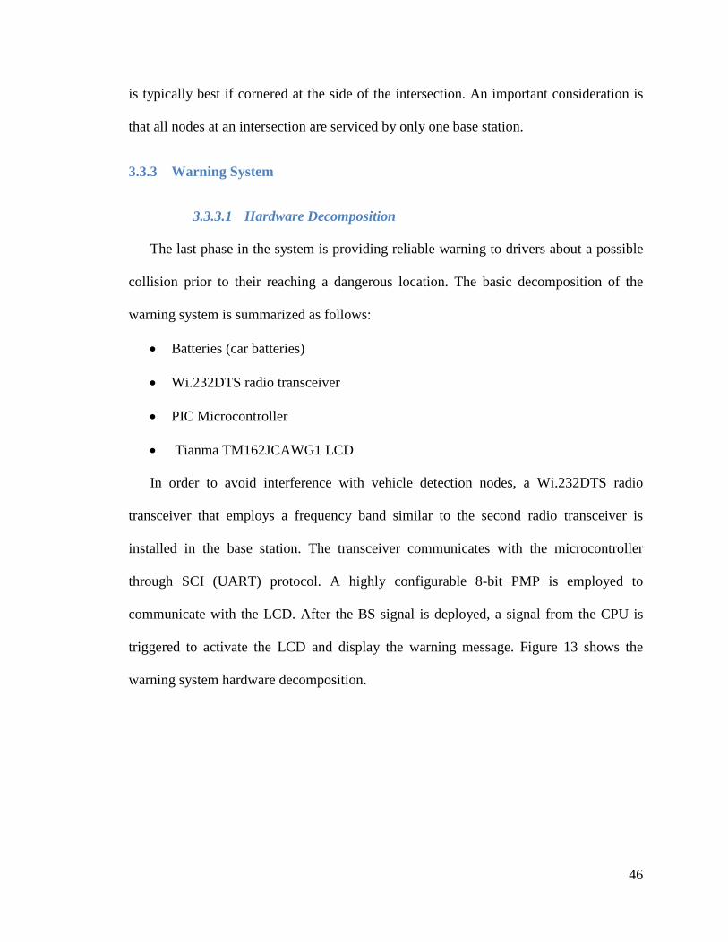
3.3.3 Warning System
3.3.3.1 Hardware Decomposition
The last phase in the system is providing reliable warning to drivers about a possible
collision prior to their reaching a dangerous location. The basic decomposition of the
warning system is summarized as follows:
• Batteries (car batteries)
• Wi.232DTS radio transceiver
• PIC Microcontroller
• Tianma TM162JCAWG1 LCD
In order to avoid interference with vehicle detection nodes, a Wi.232DTS radio
transceiver that employs a frequency band similar to the second radio transceiver is
installed in the base station. The transceiver communicates with the microcontroller
through SCI (UART) protocol. A highly configurable 8-bit PMP is employed to
communicate with the LCD. After the BS signal is deployed, a signal from the CPU is
triggered to activate the LCD and display the warning message. Figure 13 shows the
warning system hardware decomposition.
47
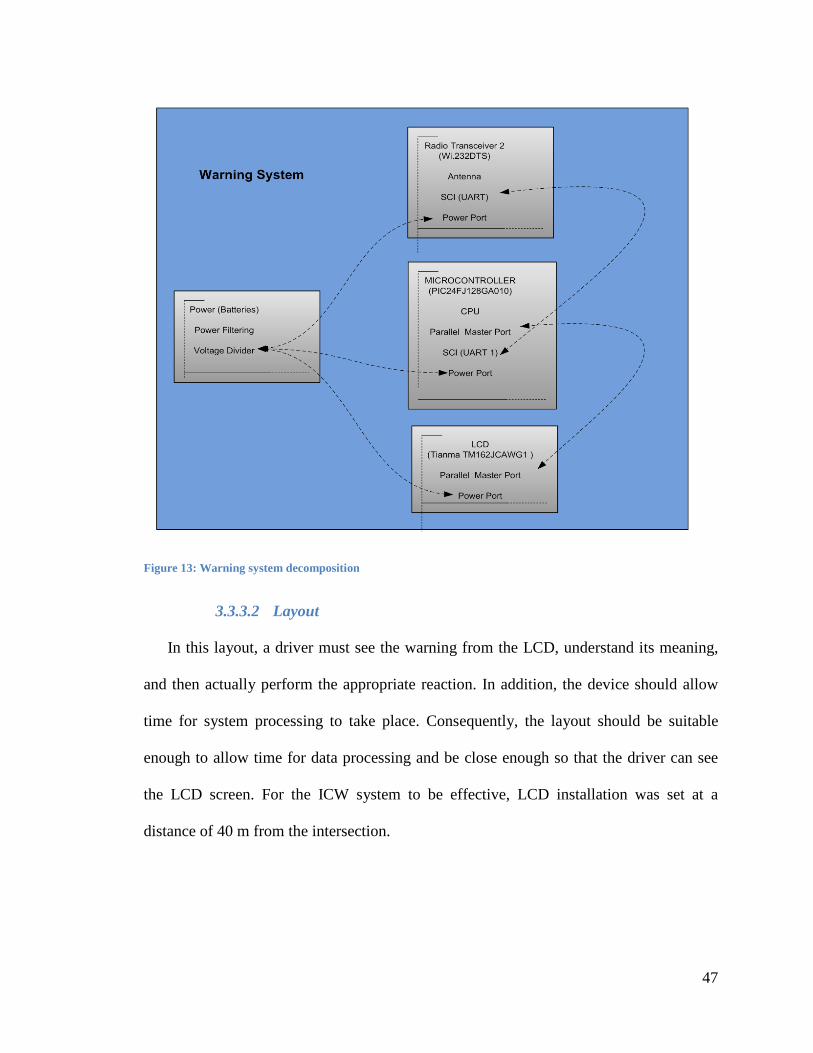
Figure 13: Warning system decomposition
3.3.3.2 Layout
In this layout, a driver must see the warning from the LCD, understand its meaning,
and then actually perform the appropriate reaction. In addition, the device should allow
time for system processing to take place. Consequently, the layout should be suitable
enough to allow time for data processing and be close enough so that the driver can see
the LCD screen. For the ICW system to be effective, LCD installation was set at a
distance of 40 m from the intersection.
48
3.4 Wireless Communication
3.4.1 Modulation
Wi232DTS employs a Frequency-shift Keying (FSK) modulation method in which
modulating the frequency of the carrier transmits digital signals. A higher bandwidth is
achieved by using a Digital Transmission System (DTS). This modulation technique
utilizes the digital spread spectrum provision employed by the Federal Communication
Commission (FCC) part 15 rules.
3.4.2 Bandwidth
Wi232DTS requires the system to use at least 500 KHz of bandwidth to achieve a
high power transmission. In DTS mode, the system uses 600 KHz of bandwidth, which
can operate on 32 different channels and operate to 100 Kbps in channel throughput.
3.4.3 Interference
Wi.232DTS uses a public 902-928 MHz transmission; therefore, interfering with
other devices is imminent. Devices that would likely interfere with the module are ones
implemented through the IEEE 802.15.4 standard. Examples of protocols that apply to
this standard include ZigBee, WirelessHART, and MiWi.
3.4.4 Range
The range of the Wi232DTS is dependent on the transmission power used.
Wi232DTS employs eight operational power modes: High Low Power (LP), Mid-High
LP, Mid-Low LP, Low DTS, High DTS, Mid-High DTS, Mid-Low DTS, and Low LP.
To determine the range of the transmission, a link budget analysis of the wireless link is
49
needed. This is calculated by adding the chosen transmit power, the antenna gains and the
receiver sensitivity [33], as shown in the following equation:
𝐿𝐿𝐿𝐿 = 𝑃𝑃𝑆𝑆𝑃𝑃 + 𝐺𝐺𝑆𝑆𝑃𝑃𝑎𝑎 − 𝑆𝑆𝑆𝑆𝑆𝑆𝑆𝑆𝑑𝑑𝑃𝑃 + 𝐺𝐺𝑑𝑑𝑃𝑃𝑎𝑎
Maximum values chosen for the Wi232DTS transceiver are characterized by the
following:
• Transmit power: 11dBm
• Antenna gains for each of the transmitter and the receiver: 3db
• Receiver sensitivity: -100dBm
A maximum link budget of approximately 117dB is capitulated, yielding more than
enough to achieve a range of 403 meters. However, as highlighted in the previous
section, the outermost deployed node is approximately 150m apart from the intersection.
Thus, the system has a maximum range of 150 m, which is acceptable in transceiver
design.
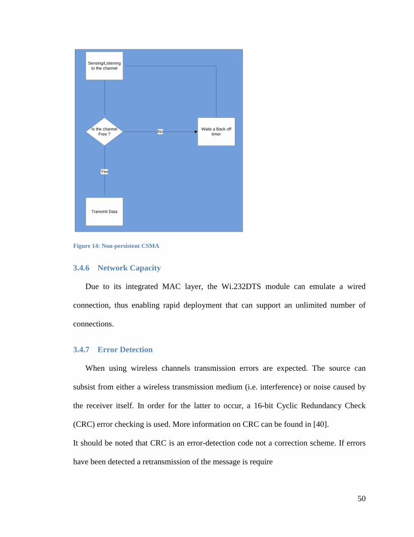
3.4.5 MAC
Non-persistent Carrier-sense multiple access (CSMA) is implemented in Wi.232DTS.
This random access technique listens to the channel before transmitting a message and
waits if another Wi.232DTS is already transmitting. After time expires the algorithm is
repeated until the channel is free. Figure 14 shows a flow chart of the implemented
algorithm.
50
Figure 14: Non-persistent CSMA
3.4.6 Network Capacity
Due to its integrated MAC layer, the Wi.232DTS module can emulate a wired
connection, thus enabling rapid deployment that can support an unlimited number of
connections.
3.4.7 Error Detection
When using wireless channels transmission errors are expected. The source can
subsist from either a wireless transmission medium (i.e. interference) or noise caused by
the receiver itself. In order for the latter to occur, a 16-bit Cyclic Redundancy Check
(CRC) error checking is used. More information on CRC can be found in [40].
It should be noted that CRC is an error-detection code not a correction scheme. If errors
have been detected a retransmission of the message is require
Sensing/Listening to the channel
Is the channel Free ?
Transmit Data
Waits a Back off timerNo
Yes
51
4 System Processing
4.1 Oscillator Select
Selecting a suitable Oscillator is the first step to processing. In doing so, two
important criteria’s should be considered: its frequency and the accuracy tolerated.
Frequency relates to the power of operation of the system, i.e. the power of the processor
and the speed afforded the job. Accuracy refers to the degree of tolerance the processor
can handle while temperature change is present. To get accurate data the stability of the
oscillator should be between -2% and +2%. This is important for the system proposed in
this report, as it will be deployed outside, where change of temperature is imminent.
PIC24FJ128GA010 employs an 8 MHz RC internal oscillator that can tolerate 32 MHz
by using PLL functionality. Such an oscillator provides high frequency, fast startup and
low cost but experiences poor accuracy over temperature variation. With constant change
in temperature, the accuracy of such a system is between -5% to +5 % [37], which is
outside the required range. To solve this problem, rather than the RC oscillator, an 8 MHz
external crystal resonator-based oscillator is chosen as the main clock source. Crystal
oscillators are well known for their clean, reliable clock signals. Consequently, an
extremely high initial accuracy that surpasses the RC oscillator is achieved
4.2 Interfacing
As shown in the system’s functional decomposition, four types of interfacing are
present:
• Asynchronous serial communication via RS232, which uses UART as the
communication interface between transceiver 1 and the PIC
52
• USB OTG module between transceiver 2 and the PIC.
• Parallel communication via PMP between LC and the PIC
• Digital I/O port between the magnetic sensor and the PIC
4.2.1 Universal Asynchronous Receiver Transmitter
UART protocol is used primarily as a communication interface for serial
communication. It is one of the oldest and simplest interfaces used in embedded-control.
4.2.1.1 Communication protocol
The most basic components for the UART interface include:
• Baud Rate Generator (BRG), i.e. the speed by which sampling the middle of a bit
period takes place
• Transmit control (UxCTS) and Receive control (UxRTS), i.e. hardware flow
control of the transmission with pins place at RF12 and RF13 respectively
• Transmit output buffer (UxTx), i.e. data output from the module in which the
buffer is utilized through RF5 pin.
• Receive input buffer (UxRx), i.e. data input of the module placed at pin RF4.
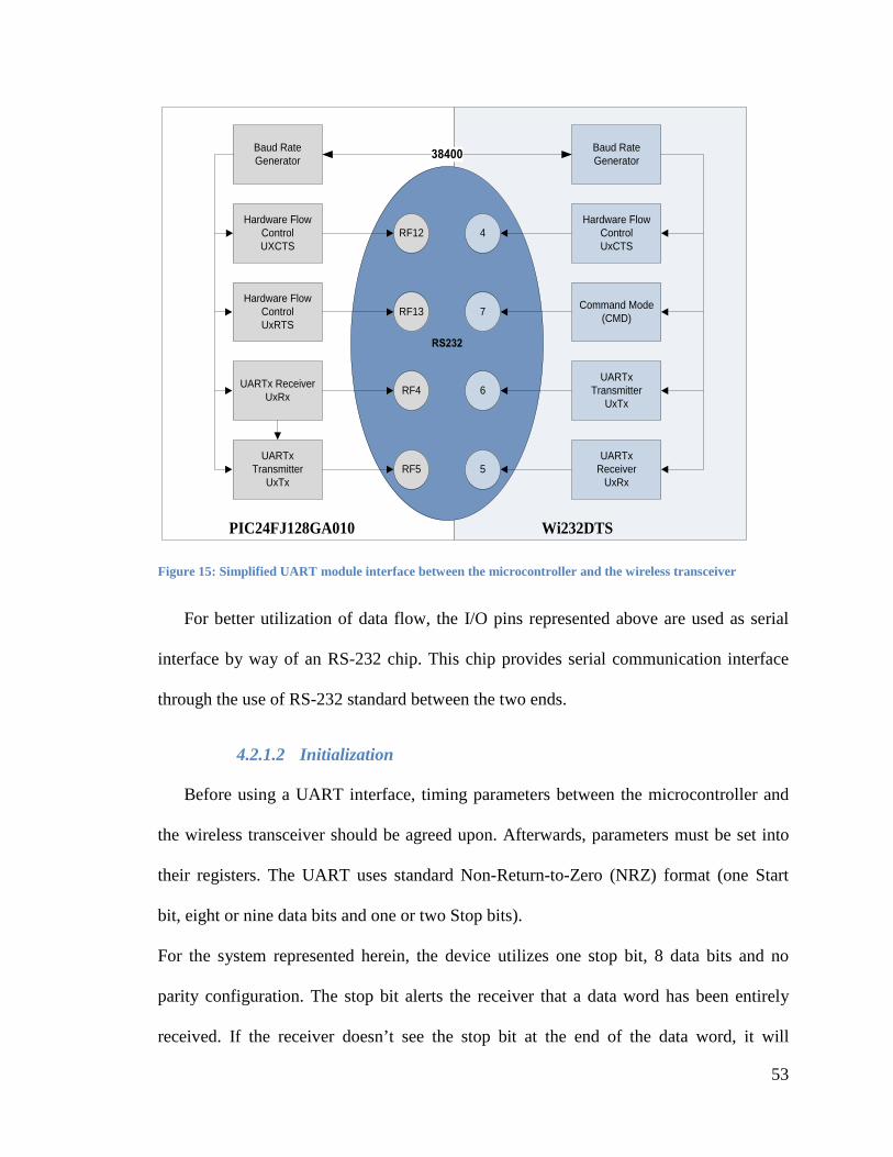
In order to establish connection between the wireless transceiver and the microcontroller,
a communication protocol should be established between the pins of the devices. Figure
15 depicts a simplified block diagram that describes the entire system interface.
53
Figure 15: Simplified UART module interface between the microcontroller and the wireless transceiver
For better utilization of data flow, the I/O pins represented above are used as serial
interface by way of an RS-232 chip. This chip provides serial communication interface
through the use of RS-232 standard between the two ends.
4.2.1.2 Initialization
Before using a UART interface, timing parameters between the microcontroller and
the wireless transceiver should be agreed upon. Afterwards, parameters must be set into
their registers. The UART uses standard Non-Return-to-Zero (NRZ) format (one Start
bit, eight or nine data bits and one or two Stop bits).
For the system represented herein, the device utilizes one stop bit, 8 data bits and no
parity configuration. The stop bit alerts the receiver that a data word has been entirely
received. If the receiver doesn’t see the stop bit at the end of the data word, it will
RS232
Baud Rate Generator
UARTx ReceiverUxRx
Hardware Flow ControlUxRTS
UARTx Transmitter
UxTx
RF13
RF4
RF5
Hardware Flow ControlUXCTS
RF12
Baud Rate Generator
UARTx Transmitter
UxTx
Command Mode (CMD)
UARTx Receiver
UxRx
Hardware Flow ControlUxCTS
7
6
5
4
PIC24FJ128GA010 Wi232DTS
38400
54
consider the data garbled and report back to the transmitter that a framing error has
occurred. Eight data bits represent the size of the data word sent through the transmission
medium. Parity bits are often used for error detection; however, they are used
infrequently to maintain system simplicity.
Baud rate is the second UART configuration parameter, i.e. the speed by which data is
sent. The higher the baud rate, the higher the data transmission speed. However, it should
be noted that higher speed is at the expense of increased Bit error rate. While
communicating, it is essential for the wireless transmitter and microcontroller to maintain
the same baud. A baud rate of 38,400 was chosen for the proposed system due to the fact
that it represents an optimal speed with an average error tolerance [41]. Additional
information about UART operations can be found at [42].
Other important criterion should be considered, the first of which is enabling the interrupt
and setting its priority in the system. This is explained in detail later.
PIC24FJ128GA010 employs a 16-bit register; therefore, to set the specified baud rate, the
value must be transformed to a BRG number that represents the microcontroller 16-bit
clock value. The equation below shows the calculation of the baud rate generator.
𝐿𝐿𝐵𝐵𝐺𝐺 = 𝐹𝐹𝐹𝐹𝐹𝐹(16∗𝐿𝐿𝑎𝑎𝐵𝐵𝑑𝑑 𝐵𝐵𝑎𝑎𝑆𝑆𝑑𝑑 )
− 1
For better understanding, the basic initialization of the UART is summarized as follows:
1. Set system clock to 8000000
2. Set FCY at SYSCLK/2
3. Set baud rate to 38400
4. Set baud rate generator to (FCY/16/BAUDRATE2)-1
5. Select one-stop bit and no parity configuration

55
6. Enable the UART module
7. Enable the transmit bit
8. Enable interrupt
9. Set interrupt priority to 6 (7 for BS)
10. Clear the receiver buffer
4.2.1.3 Transmitting and Receiving through UART
After the UART has been initialized, data can be either sent or received through the
serial communication supported. For this purpose, two 16-bit registers UxTXREG and
UxRXREG are used. U2TXREG is responsible for sending characters from the PIC to the
transceiver and can only be used when the buffer responsible for the transmission is not
full and the flag “clear to send” is raised. U2RXREG is responsible to receive characters
from the opposite end. Algorithm 1 and algorithm 2 demonstrate UART transmit and
reception.
Algorithm 1: Putting characters through UART (transmitting)
1. Set the character to be sent as T
2. Wait until the character is clear to send
3. Wait while transmitter buffer full
4. Set UxTXREG as T
56
Algorithm 2: Getting characters through UART (receiving)
1. Set the character to be received as R
2. Wait for a new character to arrive
3. Set R as UxRXREG
4.2.2 Parallel Master Port (PMP)
The use of PMP is necessary for LCD interfacing. This parallel port was created by
the PIC24 family to automate and accelerate access to a large number of external parallel
devices, one of which is LCD.
4.2.2.1 PMP interface
As mentioned earlier, most LCD’s are designed to communicate through PMP
modules. The PMP module implemented in the PIC is a parallel 8-bit bus used to
communicate with parallel devices. The module is used as an interface to 11 I/O pins
between the LCD and microcontroller. The 11 pins are represented as follows:
• Eight bidirectional data lines (pins PMD <7:0> )
• An enable strobe line (E) (pin PMRD)
• A Read/ Write selection line (R/W) (pin PMWR)
• An address line (RS) for the register selection (pin PMA0 )
Figure 16 shows how the PMP module is implemented.
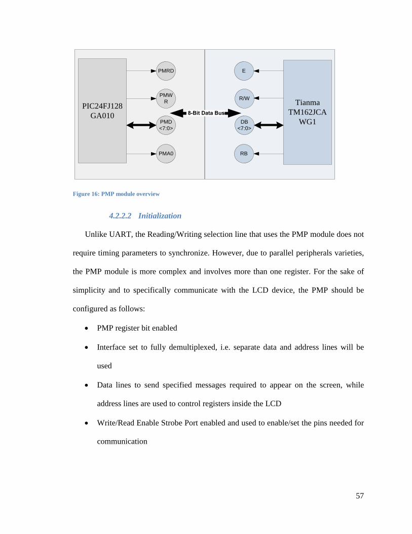
57
Figure 16: PMP module overview
4.2.2.2 Initialization
Unlike UART, the Reading/Writing selection line that uses the PMP module does not
require timing parameters to synchronize. However, due to parallel peripherals varieties,
the PMP module is more complex and involves more than one register. For the sake of
simplicity and to specifically communicate with the LCD device, the PMP should be
configured as follows:
• PMP register bit enabled
• Interface set to fully demultiplexed, i.e. separate data and address lines will be
used
• Data lines to send specified messages required to appear on the screen, while
address lines are used to control registers inside the LCD
• Write/Read Enable Strobe Port enabled and used to enable/set the pins needed for
communication
PIC24FJ128GA010
PMD <7:0>
PMA0
8-Bit Data Bus
Tianma TM162JCA
WG1
RB
DB <7:0>
PMWR
PMRD
R/W
E
58
• Master mode 1 is set with Read and Write signals on the same pin; to control the
flow of information, a second control line is set to determine when a read or write
action will take place.
• Enable the use of 8-bit, rather than 16-bit bus interface (The bus is used as a
support for the length of the data sent through the transmission medium. and the
choice is based on author’s personal preferences.)
• Read/Write data set for long waits (LCD devices are usually extremely slow;
therefore, longer waits are needed for communication.)
• Interrupts enabled with priority set to 7, i.e. highest (This will be discussed later
in the chapter.)
4.2.2.3 Writing through the PMP module
The chosen LCD module (Tianma TM162JCAWG1) is HD44780 compatible. This
means that the LCD controller contains two registers: one for sending data and the other
for control. In order to use the fist register, data has to be sent in ASCII format. This is
controlled by the PMDIN1 register in the microcontroller. The second register is
controlled by PMADDR in the microcontroller. If the value of the control register is 1,
the value used for PMDIN1 is used as display characters on the LCD. However, if the
value is 0, the data sent through PMDIN1 is for instructions only. These represent explicit
commands to the LCD to perform certain functionality, such as clear, display and go to
next line. For more information about commands, refer to document [43].
Algorithm 3 shows how to write to the LCD.

59
Algorithm 3: Writing data to the LCD module
1. Set addr as the value of the control register
2. Set C as the value of data
3. Wait until LCD is not busy
4. Wait for availability of PMP module
5. Set PMADDR as addr
6. Set PMDIN1 as C
4.2.3 Digital I/O port
An I/O port is used as an interface between the magnetic sensor and the
microcontroller. As stated earlier, the magnetic sensor uses a comparator to transform the
analog signal to a digital one based on a given threshold. Hence, the interfacing process is
straight-forward and simple to implement. Because the functionality of the magnetic
sensor is merely to signal whether or not a vehicle has passed through the sensor field,
the system needs only one digital input I/O port to fetch its signal. The chosen I/O port
for the system is RD8. It is important to note that the system utilizes input capture
interrupts to collect the signal. More about this will discussed later.
4.3 Interrupts
An “interrupt” is characterized as an internal or external event that requires quick
attention from the CPU. The PIC24 architecture provides a rich interrupt system that can

60
manage as many as 118 distinct sources of interrupts. Each source can have a unique
piece of code, namely the Interrupt Service Routine (ISR). Three important things must
be considered when activating an interrupt in a microcontroller:
1. Interrupts has to be enabled
2. For interrupt management, a priority must be set for each interrupt.
3. Interrupt flag cleared, in initialization and after use
Several types of interrupts will be used in the system:
• Timer1 interrupt: The timer module is a 16-bit timer and can either serve as a time
counter for the Real-Time Clock or operate as a free-running interval
timer/counter
• Timer 1 can operate in sleep mode conditions by utilizing the secondary
oscillator. The most notable parameters in this module are its Period Register one
(PR1) and TMR1 values. When Timer1 interrupt is enabled, the time period is
loaded into the PR1 register. TMR1 is initially set to zero and continues to
increase in increments until it reaches the PR1 value. The Timer1 interrupt occurs
the instant the two values are equal.
• The Input Capture interrupt is defined when a change of state from 0 to 1 occurs
at a specified I/O port, thus the interrupt routine is serviced. As mentioned earlier,
the I/O port will provide the interface between the magnetic sensor and the
detection node microcontroller. When a vehicle passes, a digital signal is
transmitted through the port. If the signal is high, the interrupt is enabled, causing
the system to detect to the approaching vehicle. Because the system is time
61
sensitive, the priority of such an interrupt should be set to the maximum level,
enabling the detection functionality in the detection nodes the highest priority
among other interrupts.
• UART interrupts are used to inform the PIC about incoming data from the
transceiver and are only used when there is incoming data from the UART.
4.3.1 Power Efficiency Methodology
Energy efficiency has been a significant issue in wireless sensor network [44].
The detection nodes deployed in an intersection are in an environment where no
peripheral power is present. The nodes are installed under the road and makes replacing
the power source in the system difficult. Therefore, the nodes must use a methodology
that conserves energy and allows the system to operate for extensive periods without
wired power sources. To achieve this, two methods have been chosen: selecting suitable
transmission power and utilizing sleep mode functionality.
4.3.2 Wi232DTS Network Routing
As discussed earlier, the deployed vehicle detection nodes will communicate
directly to the BS where no use of hopping methods or mesh network technique is
needed. Consequently, the range of the system depends on the layout of the detection
nodes. This would initially give transmit space for all possible communication, foremost
the furthest node with the Base Station and the last with the vehicle.
It has been previously discussed that vehicle detection nodes will be deployed
under the road to ensure reliable sensing, and sensors will be attached to the pavement at
a low height. This system architecture causes high pass loss resulting in a diminished
communication range. Consequently, using the transmitter in a low power mode is
62
unacceptable. However, this issue may be resolved by using low power transmission to
employ a multi hopping methodology to transfer the signal. This can be easily
accomplished when each node continually shifts the data to the next nearest node until
the message eventually reaches the base station. However, according to [45], the power
consumption of a two or more hops network is much higher than a one hop system.
Additionally, the transmission delay of the data would increase due to the hops the
information must make to reach the Base Station. Consequently, a one hop network with
feasible power transmission is the best solution.
4.3.3 Power consumption
ICW is still in prototype phase; therefore, studying the power consumption for
such a system is difficult. The research would require bending the PIC, transceiver and
magnetic sensor pins out of a socket, plugging in the modules, and then subsequently
connecting a resistor to measure the current traveling through. Hence, it is suggested that
the power consumption phase be implemented when the final sensing system is designed
and ready for commercial use. For the sake of ease, an approximation of the power is
calculated through data sheets provided with components used in the system. Table 7
shows the power and current consumption at 5v for the various system components.
When the PIC goes into sleep mode, the power consumption varies with
temperature change. This is a result of variation in current. For example, at -40C, the PIC
consumes approximately 0.0002watt, while at 85C it reaches 0.003075 watt. It is
important to note that the values for power consumption presented for sleep mode in
Table 7 include an additional peripheral, these being the modules that remain running
when the PIC is in sleep mode. In the proposed system the peripherals include the RTCC,
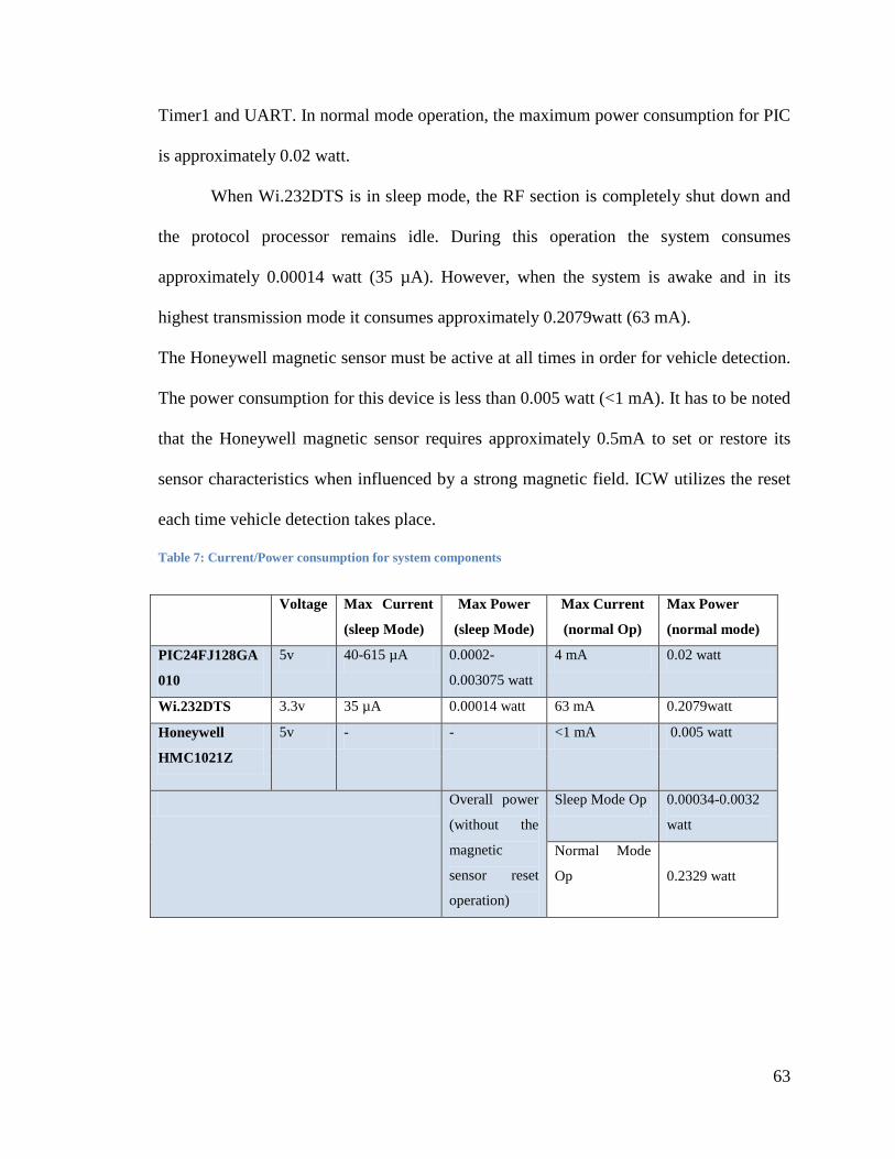
63
Timer1 and UART. In normal mode operation, the maximum power consumption for PIC
is approximately 0.02 watt.
When Wi.232DTS is in sleep mode, the RF section is completely shut down and
the protocol processor remains idle. During this operation the system consumes
approximately 0.00014 watt (35 µA). However, when the system is awake and in its
highest transmission mode it consumes approximately 0.2079watt (63 mA).
The Honeywell magnetic sensor must be active at all times in order for vehicle detection.
The power consumption for this device is less than 0.005 watt (<1 mA). It has to be noted
that the Honeywell magnetic sensor requires approximately 0.5mA to set or restore its
sensor characteristics when influenced by a strong magnetic field. ICW utilizes the reset
each time vehicle detection takes place.
Table 7: Current/Power consumption for system components
Voltage Max Current
(sleep Mode)
Max Power
(sleep Mode)
Max Current
(normal Op)
Max Power
(normal mode)
PIC24FJ128GA
010
5v 40-615 µA 0.0002-
0.003075 watt
4 mA 0.02 watt
Wi.232DTS 3.3v 35 µA 0.00014 watt 63 mA 0.2079watt
Honeywell
HMC1021Z
5v - - <1 mA 0.005 watt
Overall power
(without the
magnetic
sensor reset
operation)
Sleep Mode Op 0.00034-0.0032
watt
Normal Mode
Op
0.2329 watt
64
4.3.4 Sleep Mode
The wireless sensor network takes advantage of sleep mode functionality to
conserve power, thus power consumption is reduced to a minimum when data processing
is not needed. Placing the system in sleep mode will result in cutting off power to
unnecessary node parts, achieving the lowest energy consumption for the system.
Two system components in ICW utilize the sleep functionality, namely the
microcontroller and the transceiver. It is not possible for the magnetic sensor to go into
sleep mode, as it is the source of detection. The digital signal taken from the comparator
is therefore used to wake up the other system components.
Setting the PIC into sleep mode is straight-forward by changing the PWRSAV instruction
to zero. Updating this value will automatically shutdown the oscillator clock. As
discussed earlier in the section on interrupt, the interrupts are used to wake up the system.
In the previous section, it was mentioned that the Wi.232DTS radio transceiver is
interfaced with PIC through UART protocols. In order to set the following transceiver to
sleep mode, commands must be sent from the PIC to the radio via the selected interface.
Therefore, the methodology is a bit more complicated. The user must first set the UART
CMD pin to low, making sure that the UART data is routed to the command parser rather
than the wireless interface. Afterwards, a 0x01 command is sent from the PIC through the
UART to set the regSLPMODE (0x58) register in the transceiver. The same algorithm is
used to wake the system; however, instead of setting the regSLPMODE (0x58) to 0x01, a
command sequence of “0x0F, 0xFF, 0xFF” is sent to the same register. To verify whether
or not the Wi.232DTS is up, the module will send an acknowledgement character (0x06)
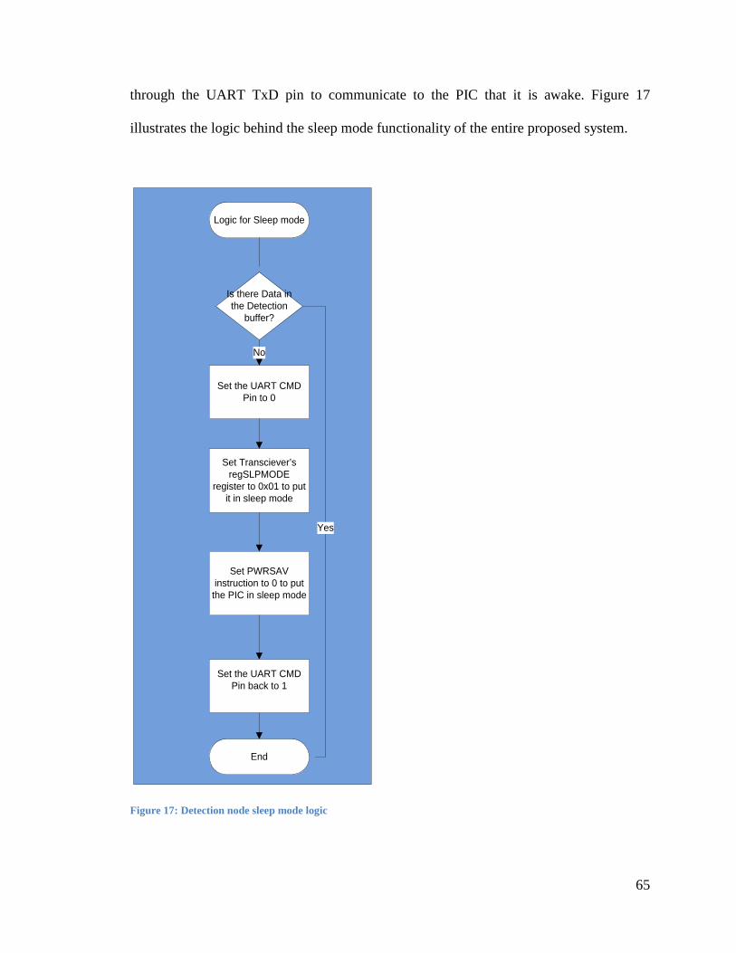
65
through the UART TxD pin to communicate to the PIC that it is awake. Figure 17
illustrates the logic behind the sleep mode functionality of the entire proposed system.
Figure 17: Detection node sleep mode logic
Set Transciever’s regSLPMODE
register to 0x01 to put it in sleep mode
Set PWRSAV instruction to 0 to put
the PIC in sleep mode
Set the UART CMD Pin to 0
Set the UART CMD Pin back to 1
Logic for Sleep mode
End
Is there Data in the Detection
buffer?
No
Yes

66
4.4 Vehicle Trajectory Prediction
In order to potentially prevent collisions, the system must have a reasonable time
prediction algorithm that can estimate the trajectories of the cars while going through an
intersection. To detect the time by which the car reaches an intersection, a function of
velocities plus accelerations measurements should be available to the BS. However, those
information are dependent of the driver’s behavior, thus they are constantly changing.
To get enough measurements, the system employs four detection nodes that are
embedded on the ground. The node’s main functionality is to sense the car and afterwards
send the time of detection to the base station. Consequently four time periods of the same
car are taken based on a predefined distance. Using the following two dimensional
motion model:
𝑑𝑑 = 𝑣𝑣𝑣𝑣 ∗ ∆𝑆𝑆 + (12∗ 𝑎𝑎 ∗ ∆𝑆𝑆2)
the time of arrival of the car to the intersection and time of its exit can be approximated.
The algorithm is as follows:
Consider the following:
• t1 represents time captured by the first node
• t2 represents time captured by the second node
• t3 represents time captured by the second node
• t4 represents time captured by the second node
• 𝑑𝑑𝑑𝑑𝑖𝑖 valued 125 m, represents the separated distance between the last node and the
entrance of the intersection.
• 𝑑𝑑𝑑𝑑𝑃𝑃 valued 135 m, represents the separated distance between the last node and the
exit of the intersection

67
Two accelerations (𝑎𝑎1 and 𝑎𝑎2 ) and two velocities (𝑉𝑉i1 and 𝑉𝑉i2) can be calculated in the
following manner:
𝑎𝑎1 = 2∆1∗ ((∆𝑆𝑆2 ∗ ∆𝑃𝑃1 )– (∆𝑆𝑆1 ∗ ∆𝑃𝑃2 ))
𝑎𝑎2 = 2∆2∗ ((∆𝑆𝑆3 ∗ ∆𝑃𝑃2 )– (∆𝑆𝑆2 ∗ ∆𝑃𝑃3 ))
𝑉𝑉i1 = 1∆1∗ ((−∆𝑆𝑆2
2 ∗ ∆𝑃𝑃1 ) + (∆𝑆𝑆2 2 ∗ ∆𝑃𝑃1 ))
𝑉𝑉i2 = 1∆2∗ ((−∆𝑆𝑆3
2 ∗ ∆𝑃𝑃2 ) + (∆𝑆𝑆2 2 ∗ ∆𝑃𝑃3 ))
Where,
∆1= (∆𝑆𝑆1 2 ∗ ∆𝑆𝑆2) − (∆𝑆𝑆2
2 ∗ ∆𝑆𝑆1 )
∆2= (∆𝑆𝑆2 2 ∗ ∆𝑆𝑆3) − (∆𝑆𝑆3
2 ∗ ∆𝑆𝑆2 )
∆t1 = t2 − t1
∆t2 = t3 − t1
∆t3 = t4 − t1
After acceleration and velocity values are calculated, time of intersection entrance of the
car (𝑆𝑆𝑑𝑑𝑖𝑖) and its exit (𝑆𝑆𝑑𝑑𝑃𝑃) can be calculated by:
Where,
v = Vi 1+Vi 22
a = a1+a22
Figure 18 depicts a detailed description of the algorithm describes above.
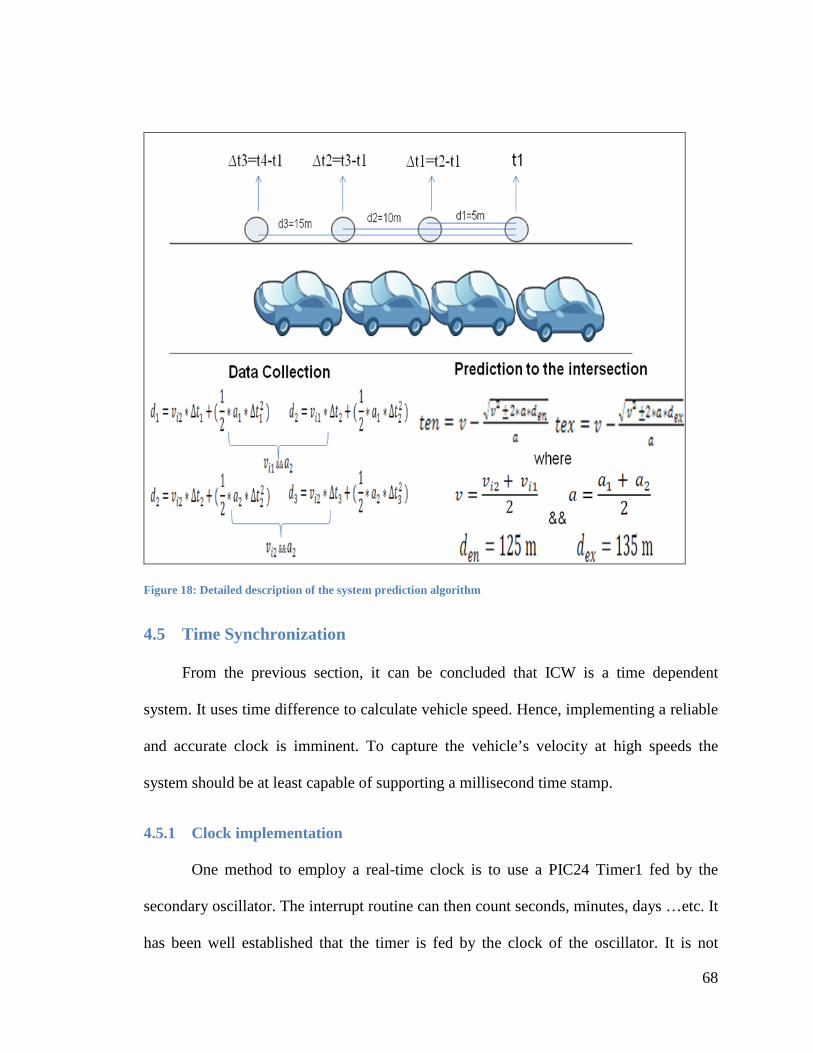
68
Figure 18: Detailed description of the system prediction algorithm
4.5 Time Synchronization
From the previous section, it can be concluded that ICW is a time dependent
system. It uses time difference to calculate vehicle speed. Hence, implementing a reliable
and accurate clock is imminent. To capture the vehicle’s velocity at high speeds the
system should be at least capable of supporting a millisecond time stamp.
4.5.1 Clock implementation
One method to employ a real-time clock is to use a PIC24 Timer1 fed by the
secondary oscillator. The interrupt routine can then count seconds, minutes, days …etc. It
has been well established that the timer is fed by the clock of the oscillator. It is not
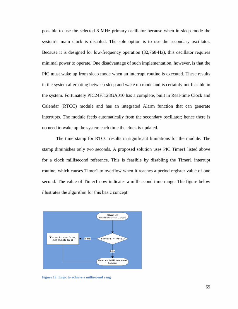
69
possible to use the selected 8 MHz primary oscillator because when in sleep mode the
system’s main clock is disabled. The sole option is to use the secondary oscillator.
Because it is designed for low-frequency operation (32,768-Hz), this oscillator requires
minimal power to operate. One disadvantage of such implementation, however, is that the
PIC must wake up from sleep mode when an interrupt routine is executed. These results
in the system alternating between sleep and wake up mode and is certainly not feasible in
the system. Fortunately PIC24FJ128GA010 has a complete, built in Real-time Clock and
Calendar (RTCC) module and has an integrated Alarm function that can generate
interrupts. The module feeds automatically from the secondary oscillator; hence there is
no need to wake up the system each time the clock is updated.
The time stamp for RTCC results in significant limitations for the module. The
stamp diminishes only two seconds. A proposed solution uses PIC Timer1 listed above
for a clock millisecond reference. This is feasible by disabling the Timer1 interrupt
routine, which causes Timer1 to overflow when it reaches a period register value of one
second. The value of Timer1 now indicates a millisecond time range. The figure below
illustrates the algorithm for this basic concept.
Figure 19: Logic to achieve a millisecond rang
Timer1 = PR1?Timer1 overflow, set back to 0 Yes
Start of Millisecond Logic
End of Millisecond Logic
No
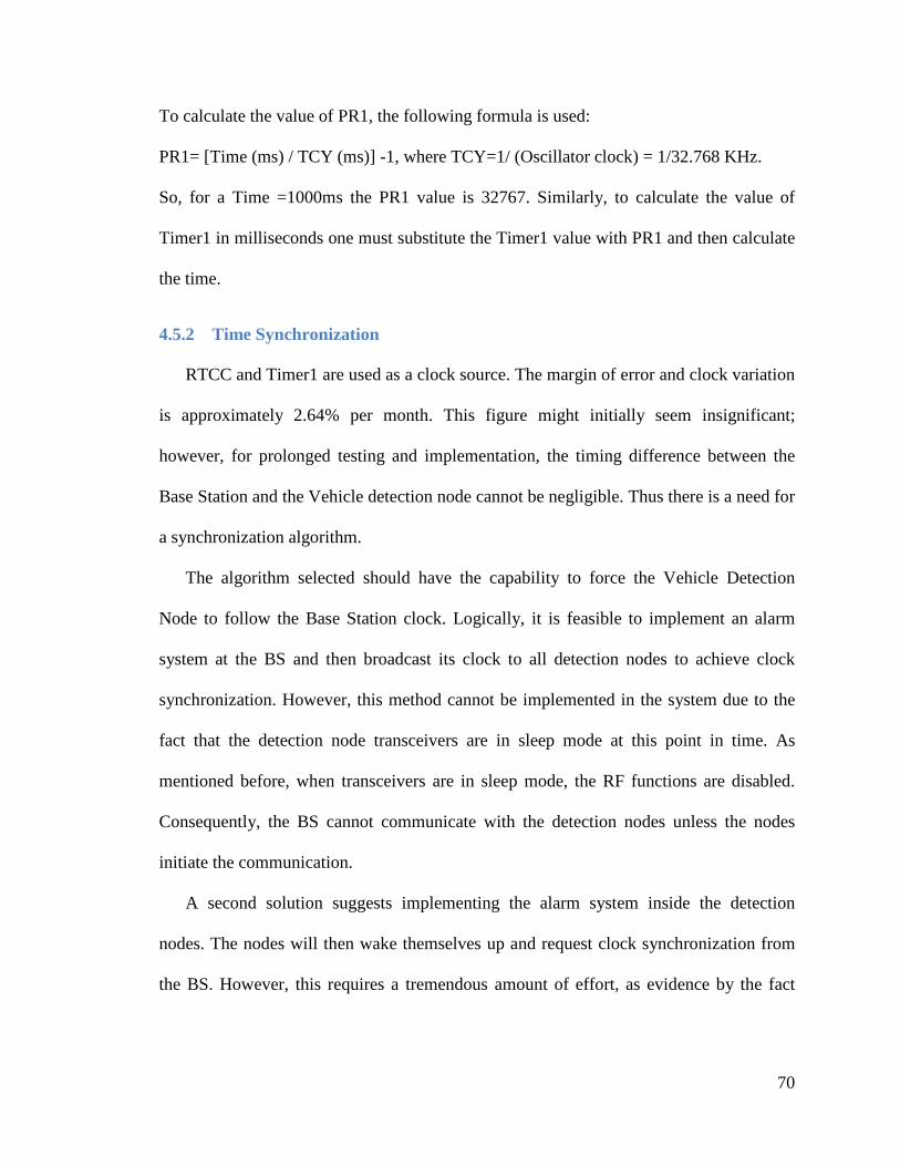
70
To calculate the value of PR1, the following formula is used:
PR1= [Time (ms) / TCY (ms)] -1, where TCY=1/ (Oscillator clock) = 1/32.768 KHz.
So, for a Time =1000ms the PR1 value is 32767. Similarly, to calculate the value of
Timer1 in milliseconds one must substitute the Timer1 value with PR1 and then calculate
the time.
4.5.2 Time Synchronization
RTCC and Timer1 are used as a clock source. The margin of error and clock variation
is approximately 2.64% per month. This figure might initially seem insignificant;
however, for prolonged testing and implementation, the timing difference between the
Base Station and the Vehicle detection node cannot be negligible. Thus there is a need for
a synchronization algorithm.
The algorithm selected should have the capability to force the Vehicle Detection
Node to follow the Base Station clock. Logically, it is feasible to implement an alarm
system at the BS and then broadcast its clock to all detection nodes to achieve clock
synchronization. However, this method cannot be implemented in the system due to the
fact that the detection node transceivers are in sleep mode at this point in time. As
mentioned before, when transceivers are in sleep mode, the RF functions are disabled.
Consequently, the BS cannot communicate with the detection nodes unless the nodes
initiate the communication.
A second solution suggests implementing the alarm system inside the detection
nodes. The nodes will then wake themselves up and request clock synchronization from
the BS. However, this requires a tremendous amount of effort, as evidence by the fact
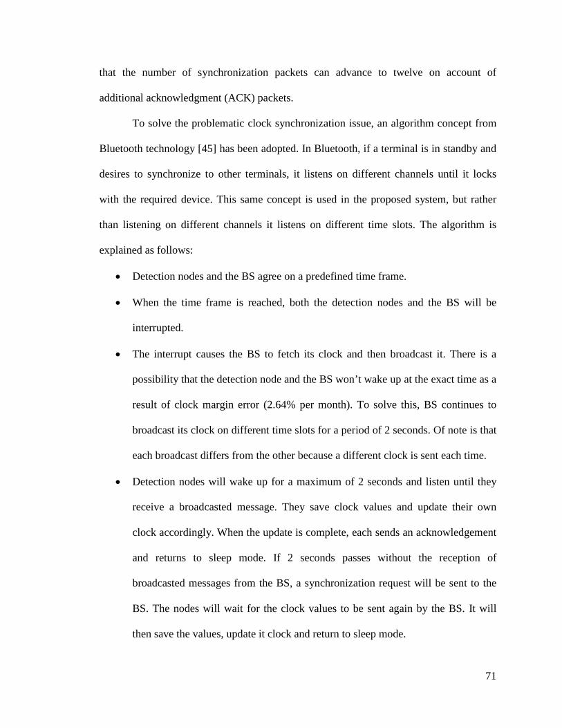
71
that the number of synchronization packets can advance to twelve on account of
additional acknowledgment (ACK) packets.
To solve the problematic clock synchronization issue, an algorithm concept from
Bluetooth technology [45] has been adopted. In Bluetooth, if a terminal is in standby and
desires to synchronize to other terminals, it listens on different channels until it locks
with the required device. This same concept is used in the proposed system, but rather
than listening on different channels it listens on different time slots. The algorithm is
explained as follows:
• Detection nodes and the BS agree on a predefined time frame.
• When the time frame is reached, both the detection nodes and the BS will be
interrupted.
• The interrupt causes the BS to fetch its clock and then broadcast it. There is a
possibility that the detection node and the BS won’t wake up at the exact time as a
result of clock margin error (2.64% per month). To solve this, BS continues to
broadcast its clock on different time slots for a period of 2 seconds. Of note is that
each broadcast differs from the other because a different clock is sent each time.
• Detection nodes will wake up for a maximum of 2 seconds and listen until they
receive a broadcasted message. They save clock values and update their own
clock accordingly. When the update is complete, each sends an acknowledgement
and returns to sleep mode. If 2 seconds passes without the reception of
broadcasted messages from the BS, a synchronization request will be sent to the
BS. The nodes will wait for the clock values to be sent again by the BS. It will
then save the values, update it clock and return to sleep mode.
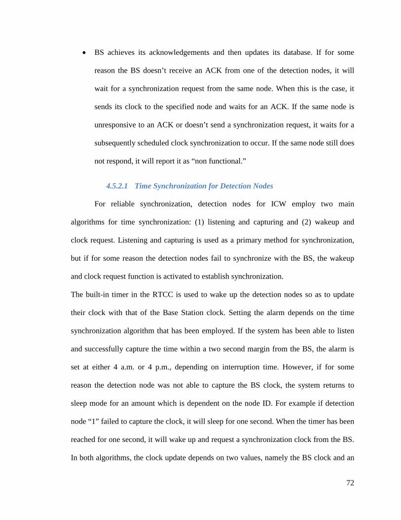
72
• BS achieves its acknowledgements and then updates its database. If for some
reason the BS doesn’t receive an ACK from one of the detection nodes, it will
wait for a synchronization request from the same node. When this is the case, it
sends its clock to the specified node and waits for an ACK. If the same node is
unresponsive to an ACK or doesn’t send a synchronization request, it waits for a
subsequently scheduled clock synchronization to occur. If the same node still does
not respond, it will report it as “non functional.”
4.5.2.1 Time Synchronization for Detection Nodes
For reliable synchronization, detection nodes for ICW employ two main
algorithms for time synchronization: (1) listening and capturing and (2) wakeup and
clock request. Listening and capturing is used as a primary method for synchronization,
but if for some reason the detection nodes fail to synchronize with the BS, the wakeup
and clock request function is activated to establish synchronization.
The built-in timer in the RTCC is used to wake up the detection nodes so as to update
their clock with that of the Base Station clock. Setting the alarm depends on the time
synchronization algorithm that has been employed. If the system has been able to listen
and successfully capture the time within a two second margin from the BS, the alarm is
set at either 4 a.m. or 4 p.m., depending on interruption time. However, if for some
reason the detection node was not able to capture the BS clock, the system returns to
sleep mode for an amount which is dependent on the node ID. For example if detection
node “1” failed to capture the clock, it will sleep for one second. When the timer has been
reached for one second, it will wake up and request a synchronization clock from the BS.
In both algorithms, the clock update depends on two values, namely the BS clock and an

73
offset. The offset is an approximated time for wireless transmission and processing.
When the clock update is successful, the node must send an ACK to the BS for
debugging purposes. If the node advances through the “Wakeup and Clock Request” a
total of three times without BS response, the detection node will assume there is a
problem with the BS.
Figure 20 shows the basic time synchronization logic for a detection node.
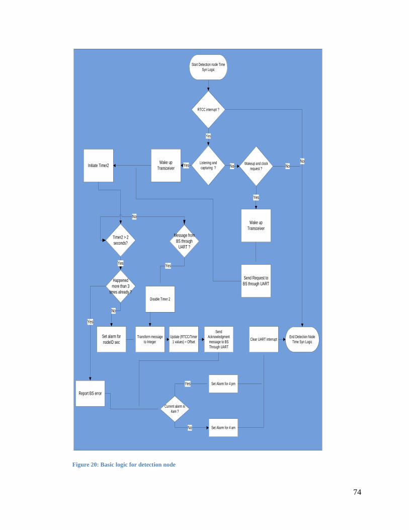
74
Figure 20: Basic logic for detection node
RTCC interrupt ?
Listening and capturing ?
Yes
Start Detection node Time Syn Logic
Wakeup and clock request ?No No
End Detection Node Time Syn Logic
YesWake up TransceiverInitiate Timer2
Timer2 > 2 seconds?
Clear UART interruptTransform message to Integer
Update (RTCC/Timer 1 values) + Offset
Send Acknowledgment message to BS Through UART
Yes
Message from BS through
UART ?
No
Yes
Send Request to BS through UART
Happened more than 3
times already ?
Set alarm for nodeID sec
No
Report BS error
Yes
Disable Timer 2
No
Wake up Transceiver
Yes
Current alarm is 4am ?
Set Alarm for 4 pm
Set Alarm for 4 amNo
Yes

75
4.5.2.2 Time Synchronization for the Base Station:
Similar to the detection nodes, the BS employs two algorithms relative to the
detection nodes: (1) regular clock broadcast and (2) clock value sent based on node
request.
Regular clock broadcast begins when an alarm set via the RTCC is activated.
Consequently, the BS broadcasts its clock for 2 seconds. It should be noted that the same
alarm is employed on the detection nodes. In so doing, the BS should expect random
ACKs from the nodes, which are used to inform the BS that the detection node has
successfully updated its clock. Because the BS in unable to broadcast and receive at the
same time, UART interrupt is enabled. This ensures that when the BS receives an ACK
from the nodes it will save the node information and continue normal broadcasting. After
the two-second margin has been reached, the BS confirms whether or not all ACKs have
been received. If they have, the BS interprets that all the nodes have updated their clocks.
Afterwards, the system updates its alarm mechanism, clears the RTCC interrupt and exit.
However, if the BS failed to receive all ACKs within the two-second time margin, it
verifies whether or not the specified nodes have failed to give an ACK at some point
during the two alarm cycles. If it indeed experienced failure, the BS will report the
specified nodes as dysfunctional. If not, it will save the information and await the second
synchronization cycle.
A small chance exists that the detection nodes won’t wake up in time to receive
the clock update. As mentioned earlier, the nodes must request clock synchronization
from the BS. When this occurs, the “clock value sent based on node request” algorithm
will initiate. The BS simply receives the request, saves the node ID, sends the clock value

76
and exits. However, the detection node must send ACK back in the same way it was
previously executed.
Figure 21 shows the basic time synchronization logic for a BS.
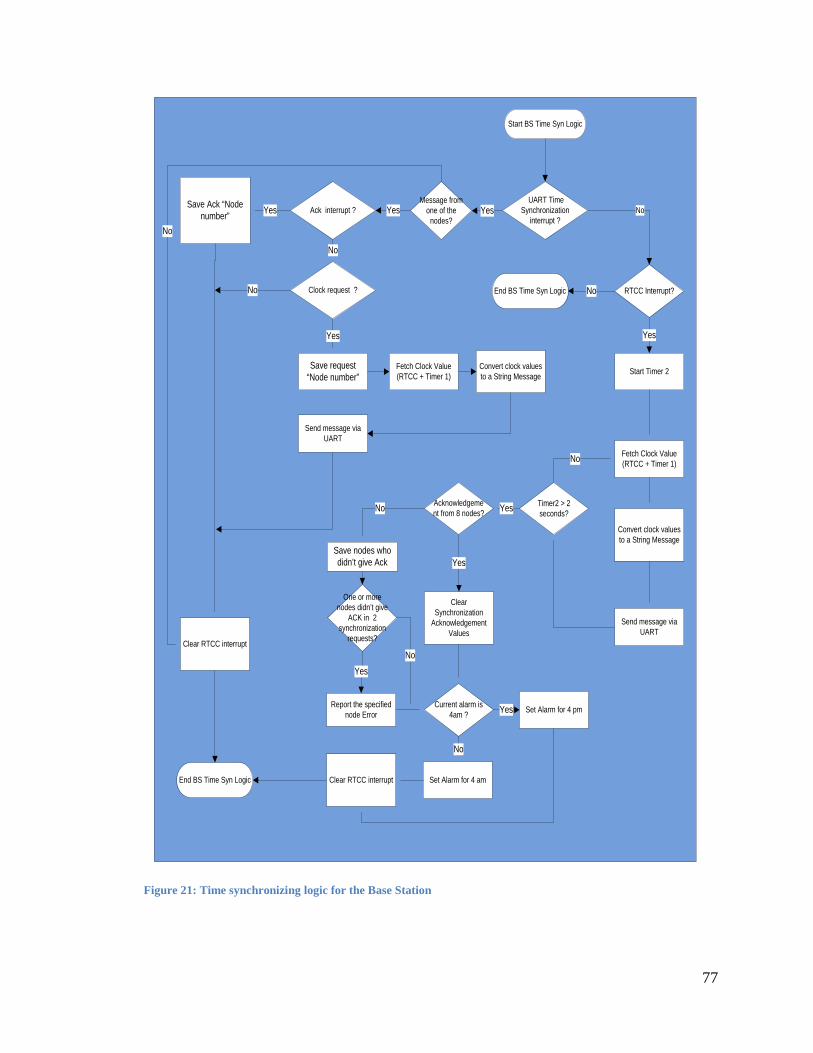
77
Figure 21: Time synchronizing logic for the Base Station
Fetch Clock Value(RTCC + Timer 1)
RTCC Interrupt?
No UART Time
Synchronization interrupt ?
Start BS Time Syn Logic
Send message via UART
Convert clock values to a String Message
Start Timer 2
Yes
Acknowledgement from 8 nodes?
Timer2 > 2 seconds?
Clear Synchronization
Acknowledgement Values
Save nodes who didn’t give Ack
One or more nodes didn’t give
ACK in 2 synchronization
requests?
Report the specified node Error
Yes
Clear RTCC interruptEnd BS Time Syn Logic
Yes
Current alarm is 4am ? Set Alarm for 4 pm
Set Alarm for 4 am
Yes
No
Save Ack “Node number” Ack interrupt ? YesYes
No
Clock request ?No
Yes
Save request “Node number”
Message from one of the
nodes?Yes
No
No Yes
No
Clear RTCC interrupt
Fetch Clock Value(RTCC + Timer 1)
Convert clock values to a String Message
Send message via UART
End BS Time Syn Logic No
No
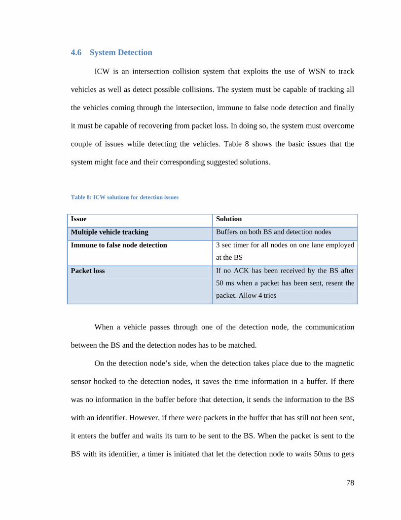
78
4.6 System Detection
ICW is an intersection collision system that exploits the use of WSN to track
vehicles as well as detect possible collisions. The system must be capable of tracking all
the vehicles coming through the intersection, immune to false node detection and finally
it must be capable of recovering from packet loss. In doing so, the system must overcome
couple of issues while detecting the vehicles. Table 8 shows the basic issues that the
system might face and their corresponding suggested solutions.
Table 8: ICW solutions for detection issues
Issue Solution
Multiple vehicle tracking Buffers on both BS and detection nodes
Immune to false node detection 3 sec timer for all nodes on one lane employed
at the BS
Packet loss If no ACK has been received by the BS after
50 ms when a packet has been sent, resent the
packet. Allow 4 tries
When a vehicle passes through one of the detection node, the communication
between the BS and the detection nodes has to be matched.
On the detection node’s side, when the detection takes place due to the magnetic
sensor hocked to the detection nodes, it saves the time information in a buffer. If there
was no information in the buffer before that detection, it sends the information to the BS
with an identifier. However, if there were packets in the buffer that has still not been sent,
it enters the buffer and waits its turn to be sent to the BS. When the packet is sent to the
BS with its identifier, a timer is initiated that let the detection node to waits 50ms to gets

79
an ACK from the BS. The detection node should expect the ACK to include the same
identifier that has been sent with the packet. By the time the detection node gets the ACK
for the specified packet; it sends the next packet in the buffer if it exits. However, if the
detection node didn’t get the ACK in the 50ms time margin due to packet loss, it will
resend the same packet again. The same packet can be sent of a maximum of four times
for a total of two seconds till the next packet waiting in the buffer gets the green light to
be sent. So, if the two seconds has been over and the packet has still not got an ACK
from the BS, the detection node will drop it and move for the next packet in the buffer if
it exits.
Figure 22 depicts the vehicle detection logic of the detection nodes.
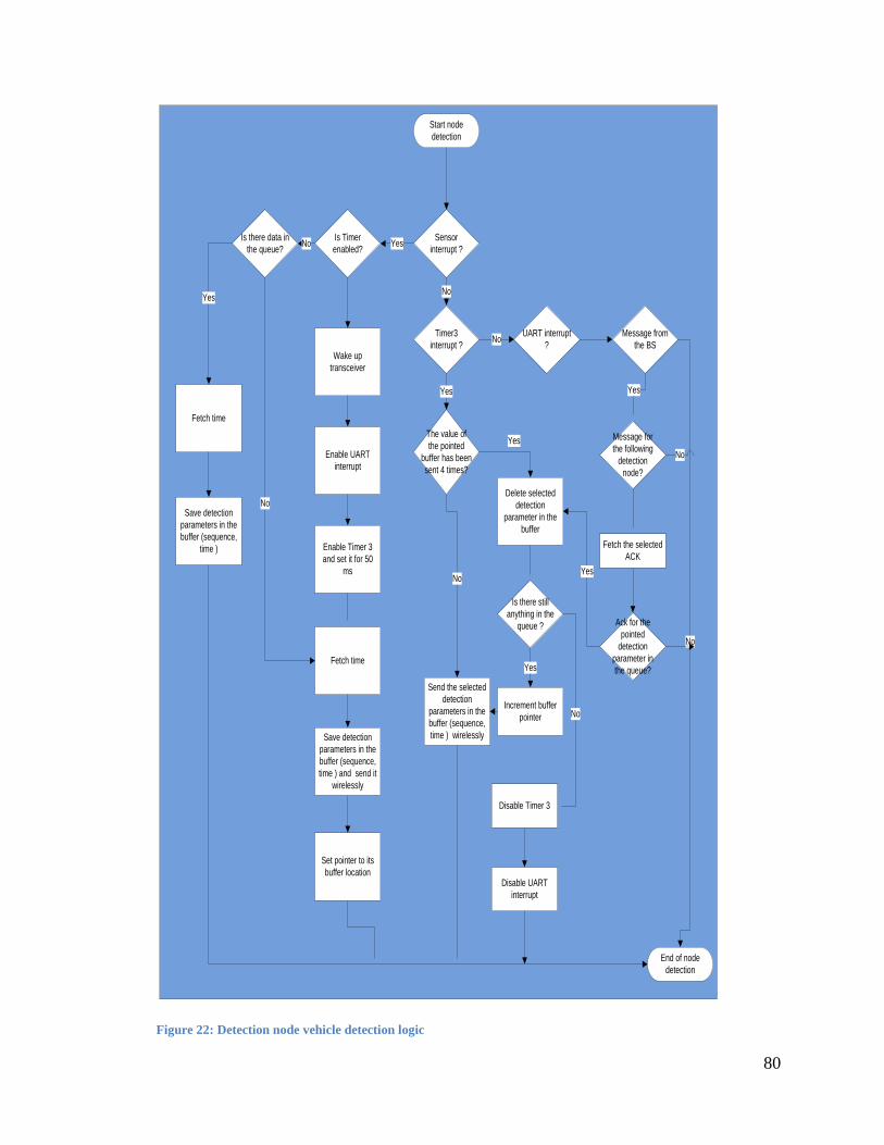
80
Figure 22: Detection node vehicle detection logic
Start node detection
Sensor interrupt ?
Is Timer enabled? Yes
Wake up transceiver
Fetch time
Enable UART interrupt
Enable Timer 3 and set it for 50
ms
NoIs there data in the queue?
No
Save detection parameters in the buffer (sequence, time ) and send it
wirelessly
Fetch time
Yes
Save detection parameters in the buffer (sequence,
time )
End of node detection
Timer3 interrupt ?
No
The value of the pointed
buffer has been sent 4 times?
Yes
Set pointer to its buffer location
Send the selected detection
parameters in the buffer (sequence, time ) wirelessly
No
Is there still anything in the
queue ?
Increment buffer pointer
Delete selected detection
parameter in the buffer
Yes
Disable Timer 3
Disable UART interrupt
UART interrupt ?No Message from
the BS
No
Message for the following
detection node?
Yes
No
Yes
No
Fetch the selected ACK
Ack for the pointed
detection parameter in the queue?
Yes

81
With respect to the BS side, when detection takes place, the BS should expect a
packet from the detection nodes with their ID in addition to the sequence of the packet.
The sequence packet is only used for packet identification. The BS has to send ACK with
the same identification ID as discussed earlier. At the BS, Detection node packets are
separated into two groups, the main lane node group and the minor lane node group. For
example, if the packet received was from node one in the main lane, the packet is saved
in the main lane node group.
Buffers at the BS are more complex that the one’s in the detection nodes. This is
simply because for each vehicle passing through the intersection, a vehicle buffer group
has to be created for it. For example if four vehicles are going through the minor lane at
the three second margin, four vehicle buffers have to be created from the same group.
The same concept goes for the main lane. This can be shown in Figure 23.
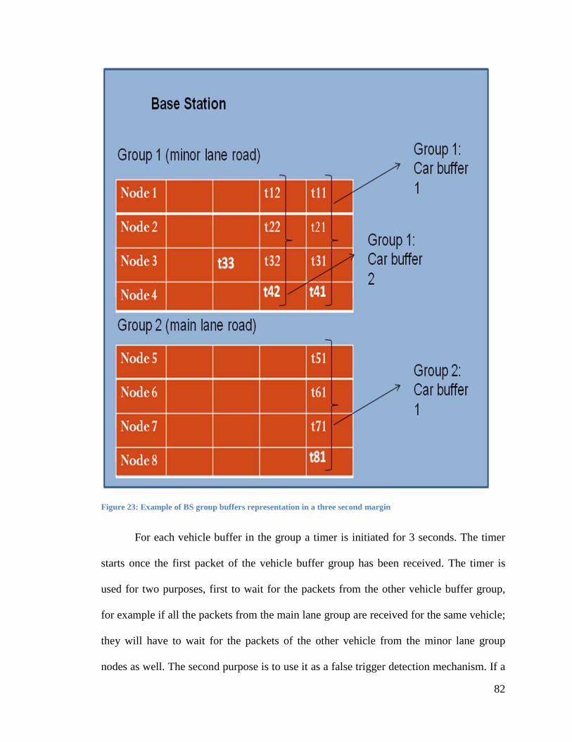
82
Figure 23: Example of BS group buffers representation in a three second margin
For each vehicle buffer in the group a timer is initiated for 3 seconds. The timer
starts once the first packet of the vehicle buffer group has been received. The timer is
used for two purposes, first to wait for the packets from the other vehicle buffer group,
for example if all the packets from the main lane group are received for the same vehicle;
they will have to wait for the packets of the other vehicle from the minor lane group
nodes as well. The second purpose is to use it as a false trigger detection mechanism. If a
83
packet is received, the BS should expect other packets from the same group nodes. If the
other nodes from the same group didn’t send any packets, the BS would assume that the
first detection was triggered by mistake. In both scenarios, once the timer has reached
without having all the info, the data will be dropped to move for other data for
processing.
To achieve data fairness, the BS processes vehicle buffers according to the time
they have been received. Once two complete vehicle buffers have been reached (one on
each group) within the three second margin, the BS will start performing “intersection
collision avoidance and warning system” analysis. More on this step will be explained in
the latter section. However, no matter the result is, whether there is a collision or not, the
system must still analyze the other vehicles values saved in the buffer within the three
second range. In doing so, a recursive algorithm is applied where each buffer in one
group is compared with another in the other group. The algorithm can be easily explained
by the following example: If we look back at Figure 23, it can be seen that there are two
vehicles in minor lane and one vehicle in the major lane. Consequently, the two vehicles
in group one should be analyzed with the vehicle in group two. The analysis is done in
the following matter: if we assume that t41 is less than t81, this means that the first
vehicle coming from group one has come before the first vehicle coming from group two.
So, after the collision analysis is made, there is no need for the data of vehicle one in
group one, simply because it has been compared with a vehicle that came after it. After
the values of vehicle one in group one (minor lane group) has been dropped, the vehicle
buffer that represents vehicle one in group two (main lane group) is compared by vehicle
two in group one. Now, if we assume that t41 is bigger than t81, the values of vehicle one

84
in group two will be dropped after the collision analysis is made. However, there is no
data in group two to be compared by group one. Thus, the vehicle buffers will be dropped
once their time margin exceeds three seconds. It has to be noted that the algorithm is
recursive, where all the buffers are going to be compared in the same manner. The overall
BS detection logic is represented in Figure 24.
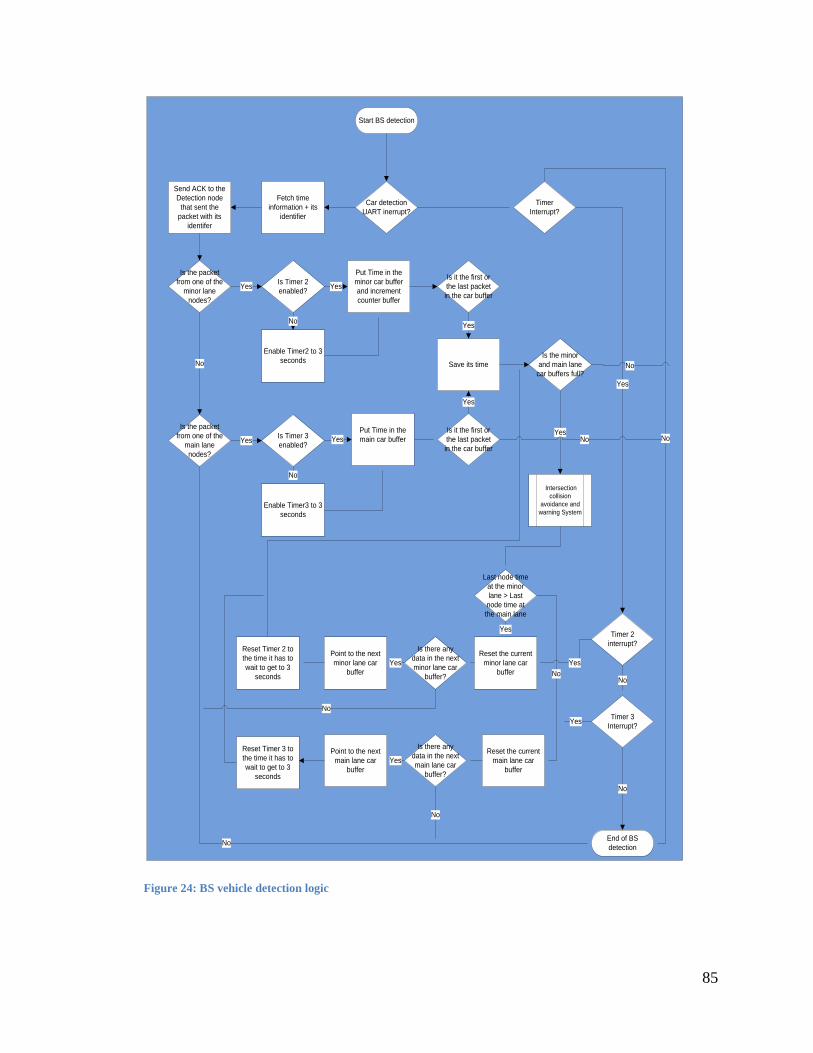
85
Figure 24: BS vehicle detection logic
Start BS detection
End of BS detection
Car detection UART inerrupt?
Fetch time information + its
identifier
Send ACK to the Detection node
that sent the packet with its
identifer
Is the packet from one of the
minor lane nodes?
Is Timer 2 enabled?Yes
Is the packet from one of the
main lane nodes?
No
No
Is Timer 3 enabled?Yes
Enable Timer2 to 3 seconds
Enable Timer3 to 3 seconds
No
No
Put Time in the minor car buffer and increment counter buffer
Yes
Put Time in the main car bufferYes
Is the minor and main lane car buffers full?
Is it the first or the last packet in the car buffer
Save its time
Yes
Is it the first or the last packet in the car buffer
Yes
Intersection collision
avoidance and warning System
Last node time at the minor lane > Last
node time at the main lane
Reset the current minor lane car
buffer
Is there any data in the next minor lane car
buffer?
Reset Timer 2 to the time it has to wait to get to 3
seconds
Point to the next minor lane car
buffer
Is there any data in the next main lane car
buffer?
Reset Timer 3 to the time it has to wait to get to 3
seconds
Point to the next main lane car
buffer
Yes
Timer Interrupt?
Reset the current main lane car
buffer
No
No
Yes
NoYes
Yes
Timer 2 interrupt?
Yes
No
Timer 3 Interrupt?
No
Yes
Yes
No
No
No
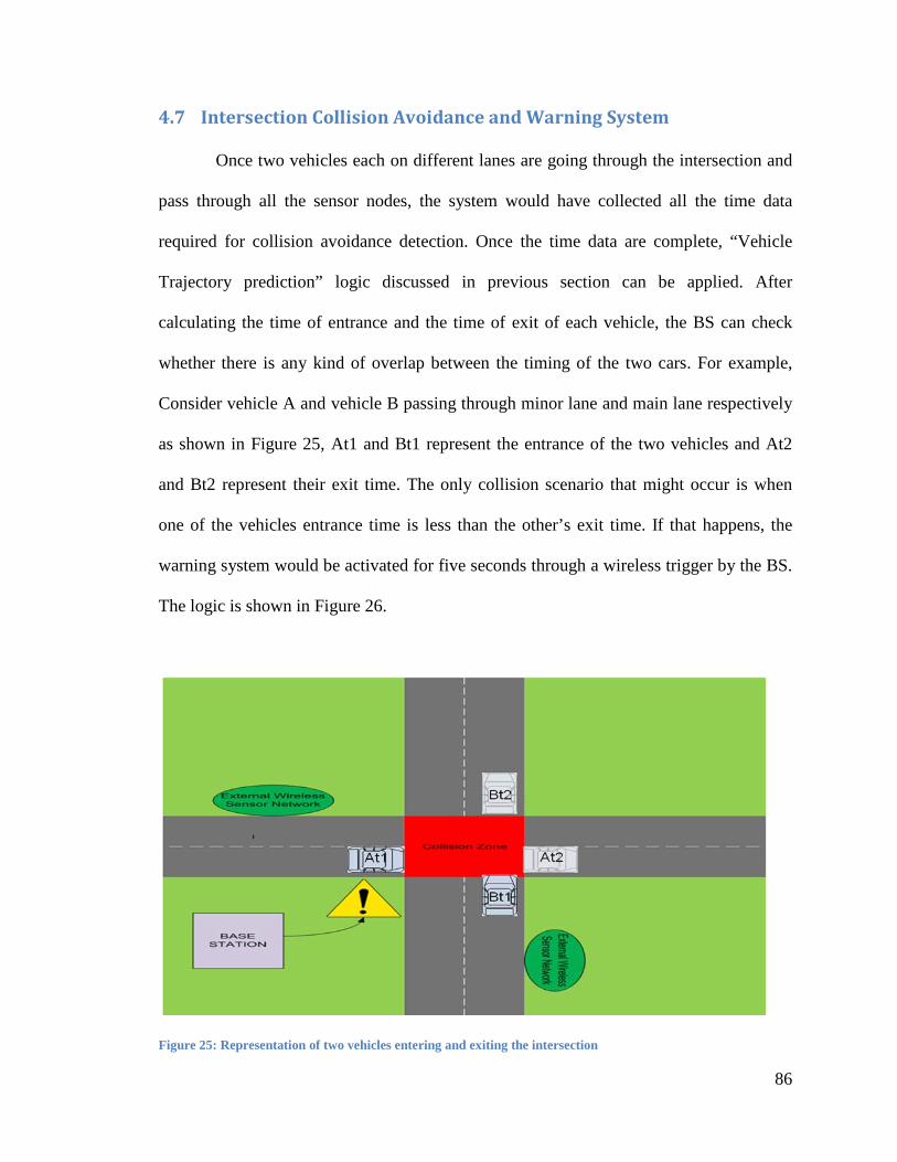
86
4.7 Intersection Collision Avoidance and Warning System
Once two vehicles each on different lanes are going through the intersection and
pass through all the sensor nodes, the system would have collected all the time data
required for collision avoidance detection. Once the time data are complete, “Vehicle
Trajectory prediction” logic discussed in previous section can be applied. After
calculating the time of entrance and the time of exit of each vehicle, the BS can check
whether there is any kind of overlap between the timing of the two cars. For example,
Consider vehicle A and vehicle B passing through minor lane and main lane respectively
as shown in Figure 25, At1 and Bt1 represent the entrance of the two vehicles and At2
and Bt2 represent their exit time. The only collision scenario that might occur is when
one of the vehicles entrance time is less than the other’s exit time. If that happens, the
warning system would be activated for five seconds through a wireless trigger by the BS.
The logic is shown in Figure 26.
Figure 25: Representation of two vehicles entering and exiting the intersection
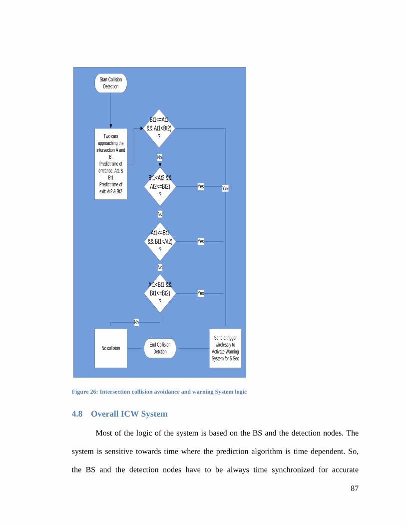
87
Figure 26: Intersection collision avoidance and warning System logic
4.8 Overall ICW System
Most of the logic of the system is based on the BS and the detection nodes. The
system is sensitive towards time where the prediction algorithm is time dependent. So,
the BS and the detection nodes have to be always time synchronized for accurate
Start Collision Detection
Send a trigger wirelessly to
Activate Warning System for 5 Sec
No collision End Collision Detction
Bt1<=At1 && At1<Bt2)
?
At1<Bt1 && Bt1<=Bt2)
?
Bt1<At2 && At2<=Bt2)
?
At1<=Bt1 && Bt1<At2)
?
No
No
No
YesYes
Yes
Yes
No
Two cars approaching the
intersection A and B.
Predict time of entrance: At1 &
Bt1Predict time of exit: At2 & Bt2
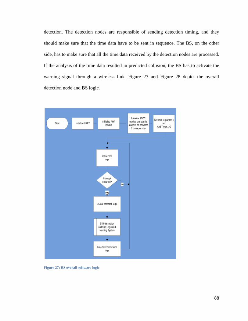
88
detection. The detection nodes are responsible of sending detection timing, and they
should make sure that the time data have to be sent in sequence. The BS, on the other
side, has to make sure that all the time data received by the detection nodes are processed.
If the analysis of the time data resulted in predicted collision, the BS has to activate the
warning signal through a wireless link. Figure 27 and Figure 28 depict the overall
detection node and BS logic.
Figure 27: BS overall software logic
Start Initialize UART Initialize PMP module
Initialize RTCC module and set the
alarm to be activated 2 times per day
Millisecond logic
Set PR1 to point to 1 sec
And Timer 1=0
Interrupt occurred?
Time Synchronization logic
BS Intersection collision Logic and warning System
No
BS car detection logic
yes
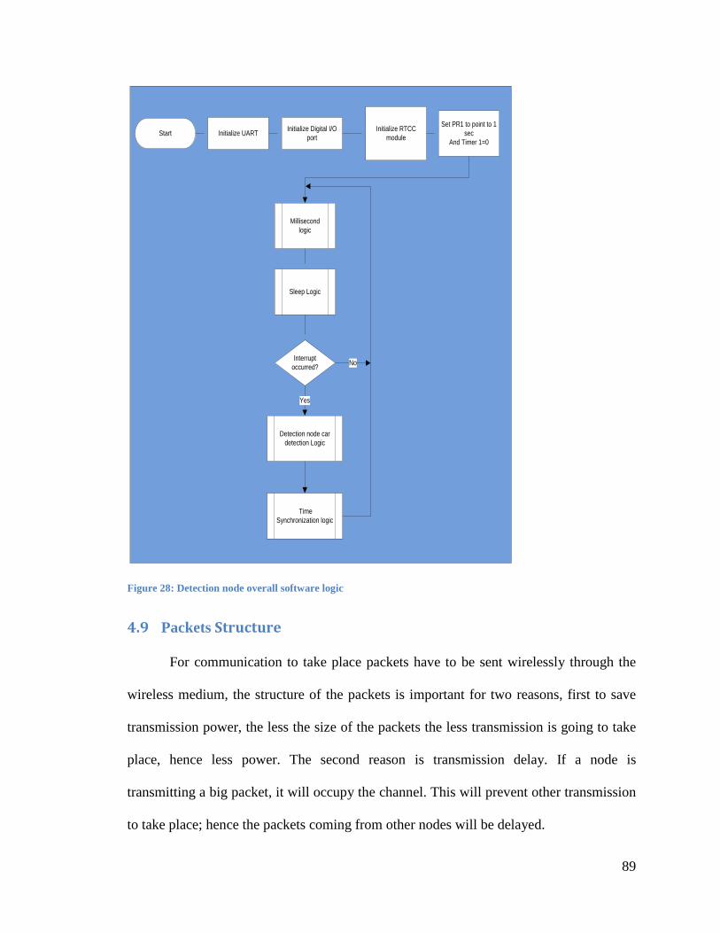
89
Figure 28: Detection node overall software logic
4.9 Packets Structure
For communication to take place packets have to be sent wirelessly through the
wireless medium, the structure of the packets is important for two reasons, first to save
transmission power, the less the size of the packets the less transmission is going to take
place, hence less power. The second reason is transmission delay. If a node is
transmitting a big packet, it will occupy the channel. This will prevent other transmission
to take place; hence the packets coming from other nodes will be delayed.
Start Initialize UART Initialize Digital I/O port
Initialize RTCC module
Millisecond logic
Set PR1 to point to 1 sec
And Timer 1=0
Interrupt occurred?
Yes
Detection node car detection Logic
Sleep Logic
No
Time Synchronization logic
90
Structure of the packets employed by ICW depends on the purpose of the
message. There are five different packet structures, three for the detection nodes and two
for the BS. All the packets include a 10 bit header as well to a 2 bit value that resembles
the purpose of the packet. The header is used by the receiver to recognize the beginning
of the packet. The packets structures are as follows:
a- Detection node packets:
- Vehicle detection packet: this is used by the detection nodes to send the time
detection information to the BS.16 bits is used to send the time information to the
BS. Only seconds and milliseconds are included in the clock value. In addition to
the time info, a 4 bit node ID and 3 bit sequence number are also employed. The
first is used by the BS to differentiate between detection nodes while the last is
used as a packet reference to be sent inside the acknowledgment packet by the
BS.
- Time request packet: Whenever the “listening and capturing” method described
in the time synchronization section fails, the detection node has to send a request
to the BS to send its clock. Once the detection nodes receive the BS clock value it
will update its clock accordingly. Additional 4 bit node ID is used as a tool for the
BS to differentiate between the detection nodes.
- Detection node acknowledgment packet: 2 bits are used by the detection nodes
to inform the BS that it has successfully updated its clock.
b- Base Station packets:
91
- Clock info packet: As described in the time synchronization section the BS has
to broadcast its clock regularly to the detection nodes. So, there is no need to
specify the packet destination (to which detection node to be sent). In addition to
a 1 bit BS ID, a 22 bit clock value is added to the packet. Minuets, seconds and
milliseconds are included in the clock value sent inside the packet.
- BS acknowledgment packet: 2 bits are used by the BS to inform the detection
node that it has successfully received its vehicle detection packet. Consequently,
the BS has to send the packet to a specified destination. A 4 bit detection node ID
is used for such a purpose. Whenever, a detection node received an
acknowledgment packet from the BS, it will check the detection node ID to its ID,
if they match then the packet is for it, otherwise it will discard it.
Figure 29 shows the different ICW packet structures.
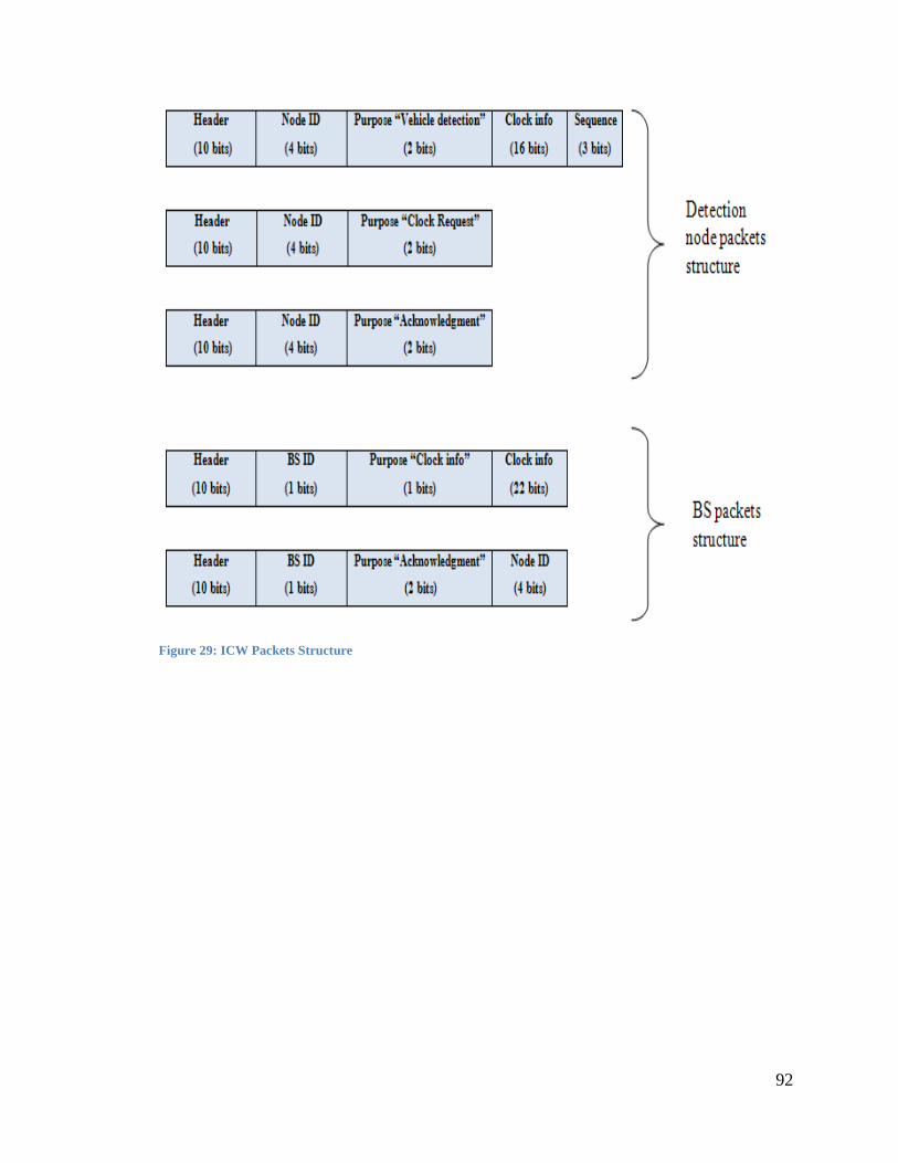
92
Figure 29: ICW Packets Structure
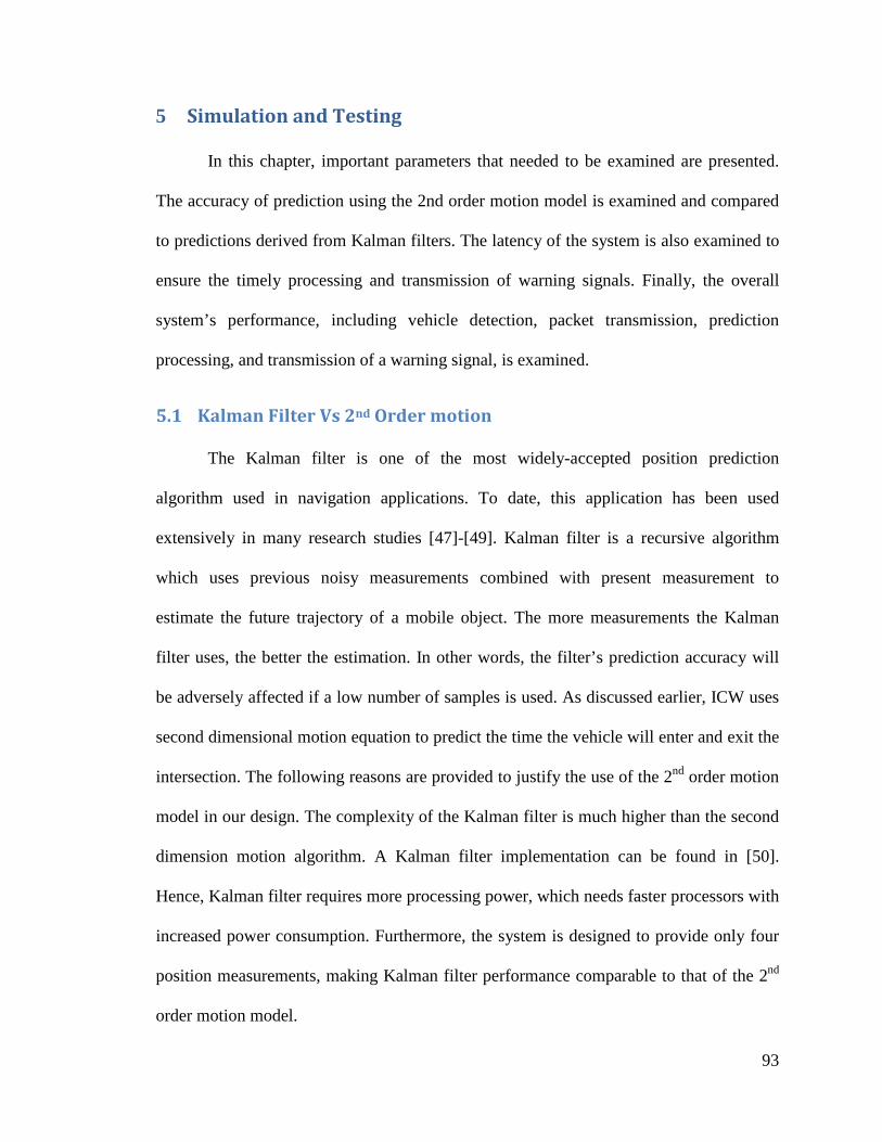
93
5 Simulation and Testing
In this chapter, important parameters that needed to be examined are presented.
The accuracy of prediction using the 2nd order motion model is examined and compared
to predictions derived from Kalman filters. The latency of the system is also examined to
ensure the timely processing and transmission of warning signals. Finally, the overall
system’s performance, including vehicle detection, packet transmission, prediction
processing, and transmission of a warning signal, is examined.
5.1 Kalman Filter Vs 2nd Order motion
The Kalman filter is one of the most widely-accepted position prediction
algorithm used in navigation applications. To date, this application has been used
extensively in many research studies [47]-[49]. Kalman filter is a recursive algorithm
which uses previous noisy measurements combined with present measurement to
estimate the future trajectory of a mobile object. The more measurements the Kalman
filter uses, the better the estimation. In other words, the filter’s prediction accuracy will
be adversely affected if a low number of samples is used. As discussed earlier, ICW uses
second dimensional motion equation to predict the time the vehicle will enter and exit the
intersection. The following reasons are provided to justify the use of the 2nd order motion
model in our design. The complexity of the Kalman filter is much higher than the second
dimension motion algorithm. A Kalman filter implementation can be found in [50].
Hence, Kalman filter requires more processing power, which needs faster processors with
increased power consumption. Furthermore, the system is designed to provide only four
position measurements, making Kalman filter performance comparable to that of the 2nd
order motion model.

94
To validate the second argument, a vehicle trajectory has been simulated. Position
predictions using Kalman filter and 2nd order motion model are compared; Figure 30 and
Figure 31 show the results of the trajectory accuracy simulations with and without
position errors, respectively. The results shown in the Figures are the average of running
the two simulations 100 times. In both simulations, a vehicle is approaching the
intersection with a velocity of 45 mph and an acceleration of 1 𝑚𝑚/𝑝𝑝2. In the simulation,
the trajectory prediction starts after passing all four detection nodes. If the nodes are five
meter apart and starting from zero as a reference, the vehicle must travel 20 meters in
order for the prediction to start. However, in the first simulation (Figure 30) no errors are
added, while in the second simulation (Figure 31), white Gaussian noise with a standard
deviation of approximately 100 ms is added. It can be concluded that the accuracy of the
Kalman and 2nd order model are about the same.
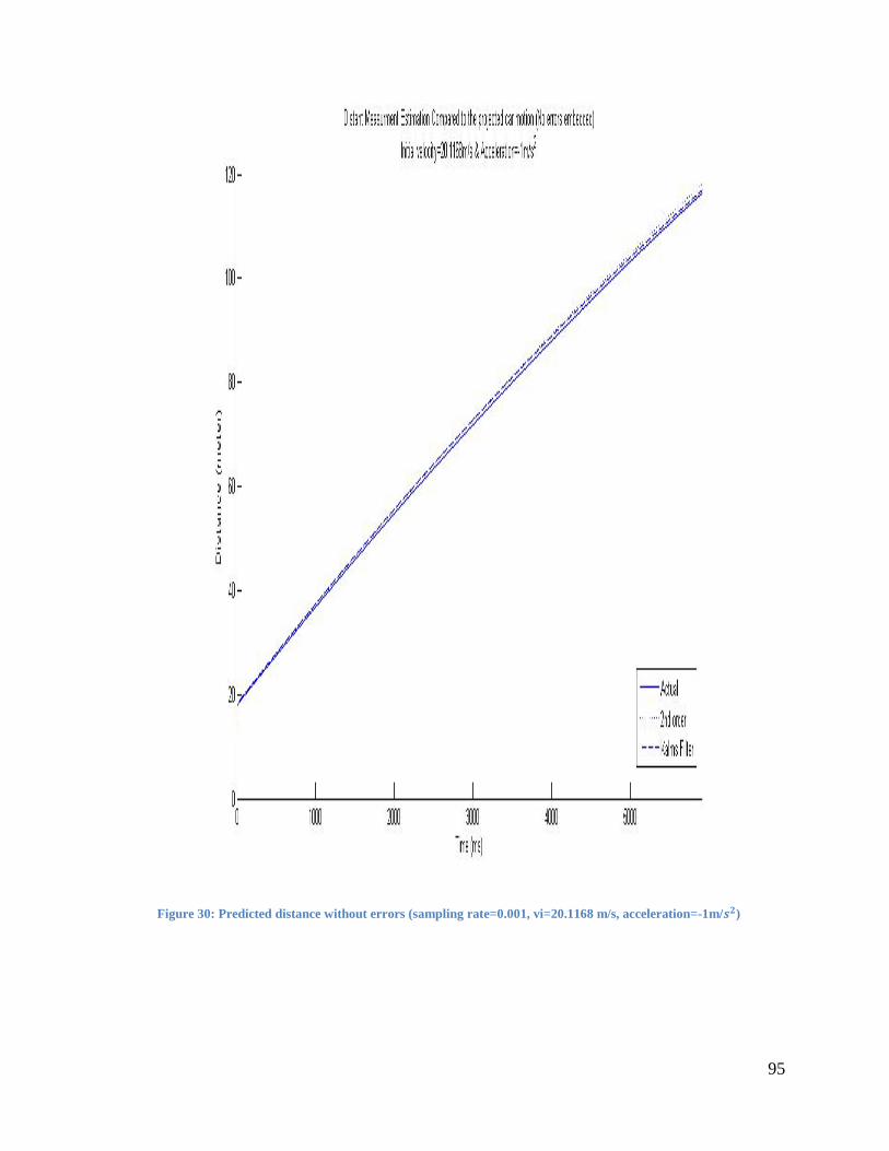
95
Figure 30: Predicted distance without errors (sampling rate=0.001, vi=20.1168 m/s, acceleration=-1m/𝒔𝒔𝒔𝒔)
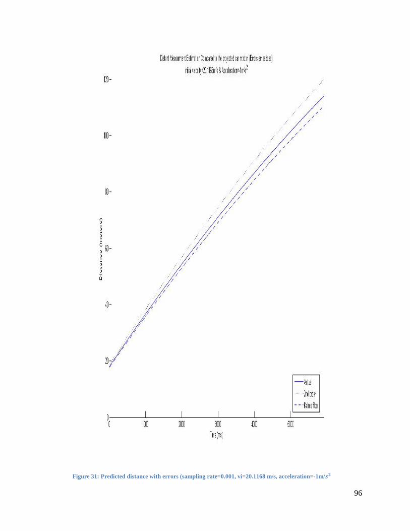
96
Figure 31: Predicted distance with errors (sampling rate=0.001, vi=20.1168 m/s, acceleration=-1m/𝒔𝒔𝒔𝒔

97
5.2 Overall System Latency
5.2.1 Analysis and Results
The overall accuracy of early and effective warning of the ICW prior to imminent
collision is the latency of the system, which includes system processing, transmission, and
propagation times. The propagation time is calculated using the speed of light and signal
travel distance between a system node and the base station. Using a maximum distance of
125 m, the time needed is approximately 4.17 ∗ 10−7 seconds, which is considered
negligible. The first tested latency is the transmission time. It refers to the time by which the
packet of data traveled from the detection node to the BS. In order to test the transmission
latency, the transceiver was placed on a loop mode. In other words, all packets transmitted
will be received by the same transceiver. A timer is added to keep track of the time sent and
received. With 100 tries, the maximum transmission latency was about 1.25ms. The resulted
latency also takes into consideration the time by which the information is delivered into the
microcontroller.
The final latency tested is the collision detection processing latency. For a real time
collision avoidance system, the driver must have sufficient time to see the warning system
and subsequently react, as well. Consequently, the processing time for collision should be as
minimal as possible. This time reflects the “Vehicle Trajectory Prediction”, “System
Detection” and “Intersection Collision Avoidance and Warning System” methods discussed
earlier in Chapter four. Through the use a timer, a trial testing comprised of 100 trials showed
that by employing the selected microcontroller (PIC24FJ128GA010), a maximum of 100 ms
is needed to estimate the time by which the each vehicle will enter and exit the intersection
and, in addition, predict whether or not there is a collision. Table 9 presents the maximum
latencies for the overall system.
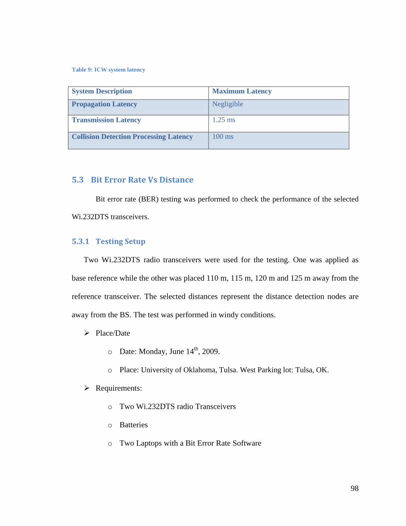
98
Table 9: ICW system latency
System Description Maximum Latency
Propagation Latency Negligible
Transmission Latency 1.25 ms
Collision Detection Processing Latency 100 ms
5.3 Bit Error Rate Vs Distance
Bit error rate (BER) testing was performed to check the performance of the selected
Wi.232DTS transceivers.
5.3.1 Testing Setup
Two Wi.232DTS radio transceivers were used for the testing. One was applied as
base reference while the other was placed 110 m, 115 m, 120 m and 125 m away from the
reference transceiver. The selected distances represent the distance detection nodes are
away from the BS. The test was performed in windy conditions.
Place/Date
o Date: Monday, June 14th, 2009.
o Place: University of Oklahoma, Tulsa. West Parking lot: Tulsa, OK.
Requirements:
o Two Wi.232DTS radio Transceivers
o Batteries
o Two Laptops with a Bit Error Rate Software
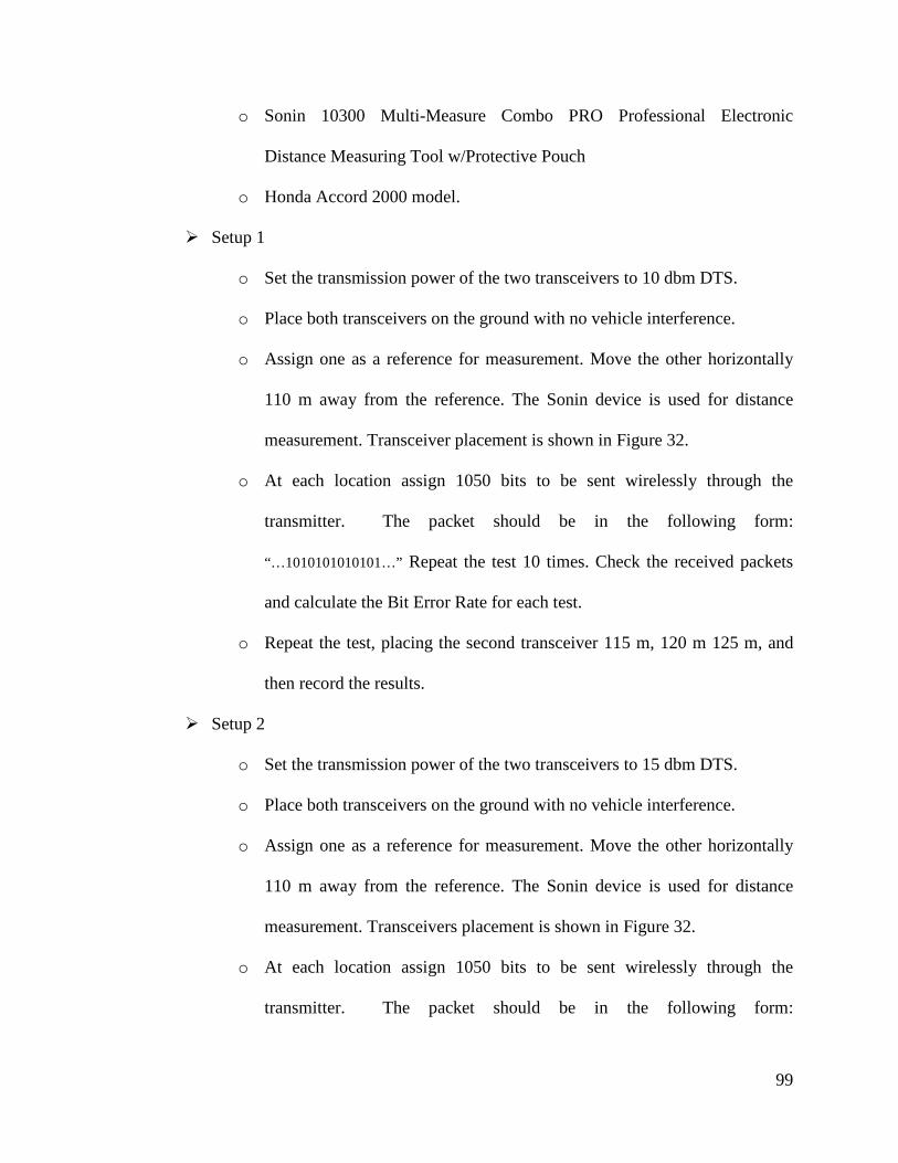
99
o Sonin 10300 Multi-Measure Combo PRO Professional Electronic
Distance Measuring Tool w/Protective Pouch
o Honda Accord 2000 model.
Setup 1
o Set the transmission power of the two transceivers to 10 dbm DTS.
o Place both transceivers on the ground with no vehicle interference.
o Assign one as a reference for measurement. Move the other horizontally
110 m away from the reference. The Sonin device is used for distance
measurement. Transceiver placement is shown in Figure 32.
o At each location assign 1050 bits to be sent wirelessly through the
transmitter. The packet should be in the following form:
“…1010101010101…” Repeat the test 10 times. Check the received packets
and calculate the Bit Error Rate for each test.
o Repeat the test, placing the second transceiver 115 m, 120 m 125 m, and
then record the results.
Setup 2
o Set the transmission power of the two transceivers to 15 dbm DTS.
o Place both transceivers on the ground with no vehicle interference.
o Assign one as a reference for measurement. Move the other horizontally
110 m away from the reference. The Sonin device is used for distance
measurement. Transceivers placement is shown in Figure 32.
o At each location assign 1050 bits to be sent wirelessly through the
transmitter. The packet should be in the following form:
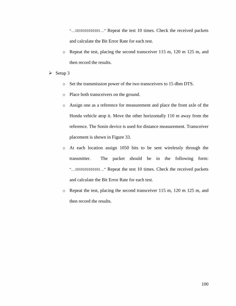
100
“…1010101010101…” Repeat the test 10 times. Check the received packets
and calculate the Bit Error Rate for each test.
o Repeat the test, placing the second transceiver 115 m, 120 m 125 m, and
then record the results.
Setup 3
o Set the transmission power of the two transceivers to 15 dbm DTS.
o Place both transceivers on the ground.
o Assign one as a reference for measurement and place the front axle of the
Honda vehicle atop it. Move the other horizontally 110 m away from the
reference. The Sonin device is used for distance measurement. Transceiver
placement is shown in Figure 33.
o At each location assign 1050 bits to be sent wirelessly through the
transmitter. The packet should be in the following form:
“…1010101010101…” Repeat the test 10 times. Check the received packets
and calculate the Bit Error Rate for each test.
o Repeat the test, placing the second transceiver 115 m, 120 m 125 m, and
then record the results.
101
Figure 32: Transceivers placement for setup 1 and 2
Figure 33: Transceivers placement for setup 3
Wi.232DTS 1Used as a reference
Line of Sight
Wi.232DTS 2Moved
horizontally
LaptopsSonin 10300 Multi-Measure Combo
PRO used for distance
measurements
Wi.232DTS 1used as a reference
Placed under the front axle of
the vehicle
Line of Sight
Wi.232DTS 2Moved
horizontally
LaptopsSonin 10300 Multi-Measure Combo
PRO used for distance
measurements
102
5.3.2 Analysis and Results
BER determines whether or not the selected distance for the nodes is acceptable.
Due to the importance of the message sent, the system cannot tolerate error. In wireless
communication a BER of 10−3 is considered acceptable.
Figure 34 depicts the BER testing results. The first test was accomplished by
setting the power of the transceivers to 10 dbm; nevertheless, the results show that with
no vehicle interference on the selected detection nodes distance, the performance of the
system was well below 10−3 . To improve the BER performance, transmission power
was increased to 15dbm. It can be seen the performance was above average on all the
selected distances with no vehicle interference. However, the vehicles are only detected
when they are above the detection nodes. Consequently, a second test was conducted to
test the effect of vehicle presence on the transceivers. As expected, vehicle interference
will degrade the performance of the system. As seen in Figure 34, with transmission
power of 15dbm added to vehicle interference, the BER increased by only a small
margin, though it is still below applying 10 dbm as a transmission power.
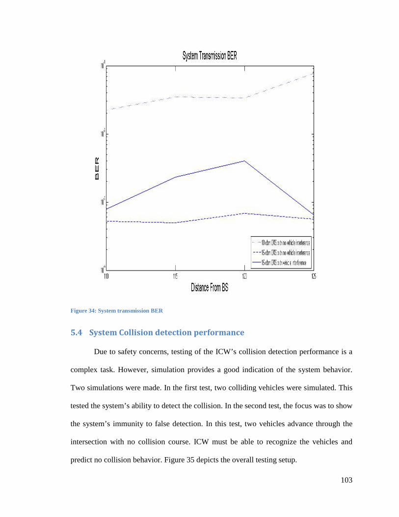
103
Figure 34: System transmission BER
5.4 System Collision detection performance
Due to safety concerns, testing of the ICW’s collision detection performance is a
complex task. However, simulation provides a good indication of the system behavior.
Two simulations were made. In the first test, two colliding vehicles were simulated. This
tested the system’s ability to detect the collision. In the second test, the focus was to show
the system’s immunity to false detection. In this test, two vehicles advance through the
intersection with no collision course. ICW must be able to recognize the vehicles and
predict no collision behavior. Figure 35 depicts the overall testing setup.
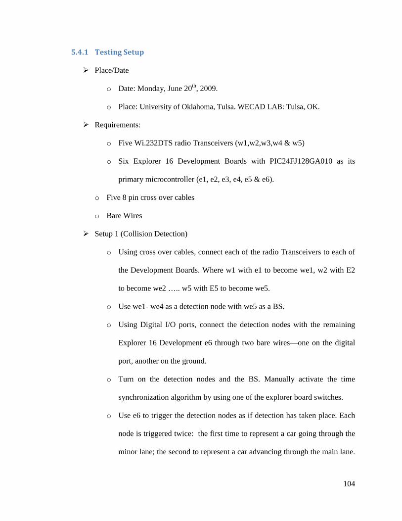
104
5.4.1 Testing Setup
Place/Date
o Date: Monday, June 20th, 2009.
o Place: University of Oklahoma, Tulsa. WECAD LAB: Tulsa, OK.
Requirements:
o Five Wi.232DTS radio Transceivers (w1,w2,w3,w4 & w5)
o Six Explorer 16 Development Boards with PIC24FJ128GA010 as its
primary microcontroller (e1, e2, e3, e4, e5 & e6).
o Five 8 pin cross over cables
o Bare Wires
Setup 1 (Collision Detection)
o Using cross over cables, connect each of the radio Transceivers to each of
the Development Boards. Where w1 with e1 to become we1, w2 with E2
to become we2 ….. w5 with E5 to become we5.
o Use we1- we4 as a detection node with we5 as a BS.
o Using Digital I/O ports, connect the detection nodes with the remaining
Explorer 16 Development e6 through two bare wires—one on the digital
port, another on the ground.
o Turn on the detection nodes and the BS. Manually activate the time
synchronization algorithm by using one of the explorer board switches.
o Use e6 to trigger the detection nodes as if detection has taken place. Each
node is triggered twice: the first time to represent a car going through the
minor lane; the second to represent a car advancing through the main lane.

105
The trigger timing should represent two cars going through minor and
main lane, both with initial velocity 40 mph and -1 𝑚𝑚/𝑝𝑝2 acceleration. For
the two cars, the timing between the nodes should be as follows:
we1 (node 1)0
we2 (node 2) 257 ms
we3(node 3) 260 ms
we4(node 4) 264 ms
o When the trigger occurs on a detection node, it should send a time stamp
and the node ID to we5 (BS) wirelessly through the transmitter. The BS
should analyze the time stamps received wirelessly from the nodes and
detect whether or not a collision will occur. However, for each detection
node in the test, there will be two IDs. For example, the first trigger will
be node 1, while the second will be node 5. In other words, each detection
node represents two nodes: one in the minor lane and the other in the
major lane.
o Check the LCD of the Explorer Board. If a warning message is sent, the
system predicted collision; if not, there is no collision. In this case, a
warning message should be displayed.
o Repeat the test 11 times.
Setup 2 (Invulnerability to false detection)
o Using the cross over cables, connect each of the radio Transceivers to each
of the Development Boards, where w1 with e1 becomes we1, w2 with E2
to become we2 ….. w5 with E5 to become we5.

106
o Use we1- we4 as a detection node, and we5 as a BS.
o Using Digital I/O ports, connect the detection nodes with the remaining
Explorer 16 Development e6 through two bare wires: one on the digital
port, another on the ground.
o Turn on the detection nodes and the BS. Manually activate the time
synchronization algorithm by using one of the switches in the explorer
boards.
o Use e6 to trigger the detection nodes as if detection has taken place. Each
node is triggered twice: the first time to represent a car going through the
minor lane, the other to represent a car going through the main lane. The
trigger timing should represent two vehicles: one represents the trajectory
of a vehicle passing through the minor lane at an initial velocity of 40 mph
and -1 𝑚𝑚/𝑝𝑝2 acceleration; the other represents a vehicle passing through
the main lane at an initial velocity of 20 mph and -1 𝑚𝑚/𝑝𝑝2 acceleration.
The triggering timing is as follows:
Minor lane simulation (vehicle moving with initial velocity 40
mph and -1 𝑚𝑚/𝑝𝑝2 acceleration)
• we1 (node 1)0
• we2 (node 2) 257 ms
• we3(node 3) 260 ms
• we4(node 4) 264 ms
Main lane simulation (vehicle moving with initial velocity 20 mph
and -1 𝑚𝑚/𝑝𝑝2 acceleration)

107
• we1 (node 1)0
• we2 (node 2) 675 ms
• we3(node 3) 747 ms
• we4(node 4) 848 ms
o When the trigger occurs on a detection node, the timestamp should be sent
wirelessly with the node ID to we5 (BS) through the transmitter. The BS
should analyze the time stamps received and detect whether or not a
collision will occur. However, for each detection node test, there will be
two IDs. For example, the first trigger will be node 1, while the second
trigger will be node 5. In other words, each detection node represents two
nodes: one in the minor lane and the other in the major lane.
o Check the LCD of the Explorer Board. A warning message signifies that
the system predicted collision. With no vehicle interference, a warning
message should not be displayed
o Repeat the test 11 times.
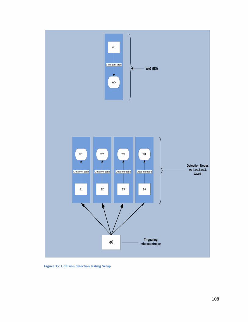
108
Figure 35: Collision detection testing Setup
e1
w1
Cross over cable
e2
w2
Cross over cable
e3
w3
Cross over cable
e4
w4
Cross over cable
e6
e5
w5
Cross over cable
Detection Nodeswe1,we2,we3,
&we4
Triggering microcontroller
We5 (BS)
109
5.4.2 Analysis and Results
Table 10 shows ICW effectiveness in the two scenarios presented. In the collision
detection test, the system showed its capability to detect collisions and, accordingly,
provide a warning. The system failed detection only once when a pointer was misplaced
in the coding, causing misplacement of packets in the buffer of the BS. However, after
this problem was fixed, consecutive testing for the same scenario resulted in successful
functioning. In the false detection invulnerability test, the results showed the system
immunity to false detection. In consecutive tests with detection, the system was able to
comprehend that the two vehicles are safe to cross the intersection, and accordingly will
not display a warning message.
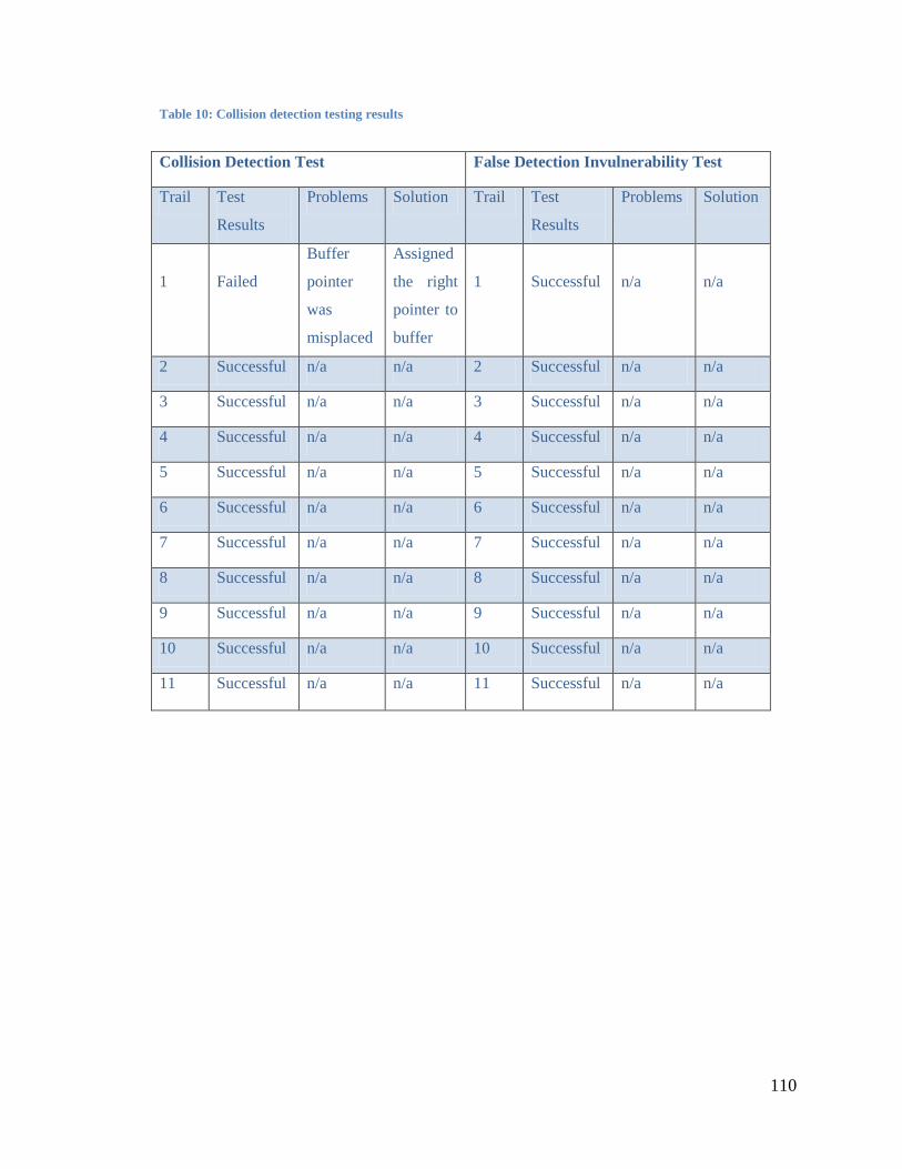
110
Table 10: Collision detection testing results
Collision Detection Test False Detection Invulnerability Test
Trail Test
Results
Problems Solution Trail Test
Results
Problems Solution
1
Failed
Buffer
pointer
was
misplaced
Assigned
the right
pointer to
buffer
1
Successful
n/a
n/a
2 Successful n/a n/a 2 Successful n/a n/a
3 Successful n/a n/a 3 Successful n/a n/a
4 Successful n/a n/a 4 Successful n/a n/a
5 Successful n/a n/a 5 Successful n/a n/a
6 Successful n/a n/a 6 Successful n/a n/a
7 Successful n/a n/a 7 Successful n/a n/a
8 Successful n/a n/a 8 Successful n/a n/a
9 Successful n/a n/a 9 Successful n/a n/a
10 Successful n/a n/a 10 Successful n/a n/a
11 Successful n/a n/a 11 Successful n/a n/a
111
6 REFERENCES
[1] Fatalities Analysis Reporting System - Encyclopedia, http://wwwfars.nhtsa.dot.gov/Main/index.aspx
[2] W. Jones, “Keeping Cars from Crashing,” IEEE Spectrum, vol. 38, no 9, pp. 40-45, 2001.
[3] W. Jones, “Building Safer Cars,” IEEE Spectrum, vol. 39, no. 1, pp. 82- 85, 2002 [4] J. Pierowicz, E. Jocoy, M. Lloyd, A. Bittner, and B. Pirson. “Intersection Collision
Avoidance Using ITS Countermeasures.” Technical Report DOT HS 809 171, NHTSA, U.S. DOT, September 2000. Final report.
[5] U.S. Department of Transportation – Federal Highway Administration and Institute of Transportation Engineers, Intersection Safety Briefing Sheets, USA, April 2004.
[6] Federal Highway Administration, http://mutcd.fhwa.dot.gov.
[7] Standard Highway Signs manual, 2004 Metric edition
“http://mutcd.fhwa.dot.gov/SHSm/regulatory.pdf”
[8] US Department of Transportation. Manual on Uniform Traffic Control Devices, rev. 2Federal Highway Administration. 2007.
[9] Arizona Department of Transportation,
“http://www.azdot.gov/Highways/traffic/Signal.asp#three”
[10] INTERSAFE, D40.4 Requirements for intersection safety applications, 28 Oct 2005.
[11] Giubbolini, L. (2000). "A multistatic microwave radar sensor for short range
anticollision warning." Vehicular Technology, IEEE Transactions on 49(6): 2270-2275.
[12] Giancarlo, A., B. Alberto, et al. (2007). "Vehicle and Guard Rail Detection Using Radar and Vision Data Fusion." Intelligent Transportation Systems, IEEE Transactions on 8(1): 95-105.
[13] Dickmanns, E. D. (2002). The development of machine vision for road vehicles in
the last decade. Intelligent Vehicle Symposium, 2002. IEEE.
[14] Wei-Chung, H., F. Li-Chen, et al. (2003). Vision based obstacle warning system for on-road driving. Intelligent Robots and Systems, 2003. (IROS 2003). Proceedings. 2003 IEEE/RSJ International Conference on.
112
[15] Gehrig, S. K. and F. J. Stein (2007). "Collision Avoidance for Vehicle-Following Systems." Intelligent Transportation Systems, IEEE Transactions on 8(2): 233-244.
[16] Jihua, H. and T. Han-Shue (2006). Design and implementation of a cooperative
collision warning system. Intelligent Transportation Systems Conference, 2006. ITSC '06. IEEE.
[17] Shie-Yuan, W., C. Yow-Wei, et al. (2008). A Vehicle Collision Warning System Employing Vehicle-To-Infrastructure Communications. Wireless Communications and Networking Conference, 2008. WCNC 2008. IEEE.
[18] Kim, M., E. Lee, et al. (2006). Simulation of Intersection Collision Avoidance
System in Wireless Sensor Networks. Geoscience and Remote Sensing Symposium, 2006. IGARSS 2006. IEEE International Conference on.
[19] Kyung Bok, S., Y. Jae Jun, et al. (2007). Collision Warning System on a Curved
Road Using Wireless Sensor Networks. Vehicular Technology Conference, 2007. VTC-2007 Fall. 2007 IEEE 66th.
[20] Menon, A., A. Gorjestani, et al. (2004). Roadside range sensors for intersection decision support. Intelligent Transportation Systems, 2004. Proceedings. The 7th International IEEE Conference on.
[21] Atev, S., O. Masoud, et al. (2005). A collision prediction system for traffic
intersections. Intelligent Robots and Systems, 2005. (IROS 2005). 2005 IEEE/RSJ International Conference on.
[22] Ashkan Sharafsaleh, Ching-Yao Chan. “Experimental Evaluation of Commercially-off-the-Shelf Sensors for Intersection Decision Support Systems.” Paper No. 1925. 12th World Congress on ITS, San Francisco. November 6-10, 2005.
[23] University of Minnesota Research: http://www.its.umn.edu/Research/ [24] Virginia Tech Transportation Institute: http://www.vtti.vt.edu/research.html
[25] King, T. I., W. J. Barnes, et al. (2007). A Wireless Sensor Network Architecture
for Highway Intersection Collision Prevention. Intelligent Transportation Systems Conference, 2007. ITSC 2007. IEEE.
[26] Kyung Bok, S., Y. Jae Jun, et al. (2007). Collision Warning System on a Curved
Road Using Wireless Sensor Networks. Vehicular Technology Conference, 2007. VTC-2007 Fall. 2007 IEEE 66th.
[27] Sensys Networks, Inc., “The Sensys wireless vehicle detection system,” System
Overview, Berkley, CA, 2007.
113
[28] Road and Trail Intersection Safety “http://www.ptny.org/pdfs/greenways/road_trails/Road%20and%20Trail%20Intersectio %20Executive%20Summary.pdf ”
[29] L. E. Mimbela, L. Klein. “A Summary of Vehicle Detection and Surveillance
Technologies used in Intelligent Transportation Systems.” Vehicle Detection Clearing House. August 31, 2007. http://www.nmsu.edu/~traffic/
[30] Traffic measurement and vehicle classification with a single magnetic sensor [31] Application Note – AN218: Vehicle Detection Using AMR Sensors.” Honeywell.
Aug. 2005. http://www.ssec.honeywell.com/magnetic/datasheets/an218.pdf [32] T. King, “A Warning System for Collision Avoidance at Highway Intersections”,
University of Oklahoma, Thesis. Electrical and Computer Engineering. 2006. [33] Radiotronix, “Wi.232DTS-FCC-RA-R,” radiotronix.com, Available:
http://www.radiotronix.com/products/proddb.asp?ProdID=197
[34] AeroComm, “Product details: AC4790 900MHz peer-to-peer transceiver modules,” aerocomm.com, Available: http://www.aerocomm.com/rf_transceiver_modules/ac4790_mesh-ready_transceiver.htm,
[35] Texas Instruments, “Z-Accel 2.4 GHz ZigBee Processor”, Available:
http://focus.ti.com/docs/prod/folders/print/cc2480a1.html [36] JAVAD, “UHF902-928”, Available:
http://storage.javad.com/downloads/manuals/modems/UHF%20902_928.pdf [37] PIC24FJ128GA010, “Product details: PIC24 16-bit Microcontroller Features,”
microchip.com, Available: http://www.microchip.com/wwwproducts/Devices.aspx?dDocName=en024805
[38] L. Itti, P. Baldi. “Bayesian Surprise Attracts Human Attention.” Neural Information Processing Systems, 2005.
[39] “General Rules Techniques and Advice for All Drivers and Riders.” 2004.
highwaycode.gov.uk. [40] Philip Koopman and Tridib Chakravarty "Cyclic Redundancy Code (CRC)
Polynomial Selection For Embedded Networks", The International Conference on Dependable Systems and Networks, DSN-2004
[41] Microchip, “Section 21. UART”, available:
http://ww1.microchip.com/downloads/en/DeviceDoc/61107D.pdf [42] Serial and UART Tutorial, Available:
http://www.freebsd.org/doc/en/articles/serial-uart/index.html
114
[43] Tianma TM162JCAWG1, Available: http://www.datasheetarchive.com/TM162JCAWG1-datasheet.html
[44] J. Polastre, R. Szewczyk, and D. E. Culler, “Telos: Enabling Ultra-Low Power
Wireless Research,” 4Th Intl. Conf. on Information Processing in Sensor Networks; Special track on Platform Tools and Design Methods for Network Embedded Sensors (IPSN ’05/SPOTS)., 2005
[45] Bjornemo, E., M. Johansson, et al. (2007). Two Hops is One too Many in an
Energy-Limited Wireless Sensor Network. Acoustics, Speech and Signal Processing, 2007. ICASSP 2007. IEEE International Conference on.
[46] Monson, Heidi (1999-12-14). "Bluetooth Technology and Implications".
SysOpt.com. [47] Messom, C. H., G. Sen Gupta, et al. (2003). Improving predictive control of a
mobile robot: Application of image processing and Kalman filtering. Instrumentation and Measurement Technology Conference, 2003. IMTC '03. Proceedings of the 20th IEEE.
[48] Wang, L.-j., J.-k. Wang, et al. (2008). Location estimation of mobile user in
wireless sensor network based on Unscented Kalman Filter. Microwave and Millimeter Wave Technology, 2008. ICMMT 2008. International Conference on.
[49] Yunpeng, Z., Z. Zhengjun, et al. (2008). An Extended Self-Adaptive Kalman
Filtering Object Motion Prediction Model. Intelligent Information Hiding and Multimedia Signal Processing, 2008. IIHMSP '08 International Conference on.
[50] R. Brown, P. Hwang. Introduction to Random Signals and Applied Kalman
Filtering, 2nd Ed. Wiley, New York. 1983. p. 230-236, 330-331.