Engineering manual No. 23

Updated: 03/2020

1

Collector lining analysis

Program: FEM

File: Demo_manual_23.gmk

The objective of this engineering manual is to perform the analysis of a mined collector with

emphasis on the lining response using the Finite Element Method.

Task specification

Determine the lining response of a mined collector; its dimensions can be seen in the following

chart. Determine the internal forces acting on the collector lining. The collector lining (0.1 m thick) is

made from reinforced concrete, class C 20/25, the bottom is at a depth of 12.0 m. The geological

profile is homogeneous; the soil parameters are as follows:

− Unit weight of soil: 𝛾 = 20.0 𝑘𝑁 𝑚3⁄

− Modulus of elasticity: 𝐸 = 12.0 𝑀𝑃𝑎

− Poisson’s ratio: 𝜈 = 0.40

− Effective soil cohesion: 𝑐𝑒𝑓 = 12.0 𝑘𝑃𝑎

− Effective angle of internal friction: 𝜙𝑒𝑓 = 21.0 °

− Unit weight of saturated soil: 𝛾𝑠𝑎𝑡 = 22.0 𝑘𝑁 𝑚3⁄

Task specification chart – mined collector

We will determine the values of displacements and internal forces only for the elastic model

because we do not expect the development of plastic deformations. We will subsequently use the

Mohr-Coulomb material model for the verification of the yield condition.

2

Solution

To analyse this task, we will use the GEO 5 – FEM program. The following paragraphs

provide a step by step description of the solution:

− Topology: setting and modelling the problem (interface, free points and lines – refining the density)

− Construction stage 1: primary geostatic stress,

− Construction stage 2: modelling beam elements, analysing displacements, internal forces

− Assessment of results: comparison, conclusion.

Topology: problem settings

In the “Settings” frame we will select the option “geostatic stress” to perform the analysis of the

construction stage 1. We will consider the problem or the analysis type as plane strain.

“Settings” frame

3

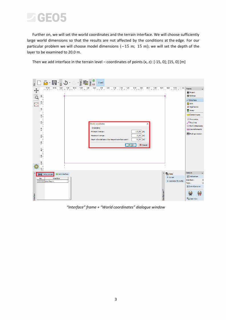
Further on, we will set the world coordinates and the terrain interface. We will choose sufficiently

large world dimensions so that the results are not affected by the conditions at the edge. For our

particular problem we will choose model dimensions ⟨−15 𝑚;  15 𝑚⟩; we will set the depth of the

layer to be examined to 20.0 m.

Then we add interface in the terrain level – coordinates of points (x, z): [-15, 0]; [15, 0] [m]

“Interface” frame + “World coordinates” dialogue window

4

Now we will specify the respective soil parameters including the material model and subsequently

we will assign the soil to the created region (for more details visit Help – F1).

“Add new soils” dialogue window

5

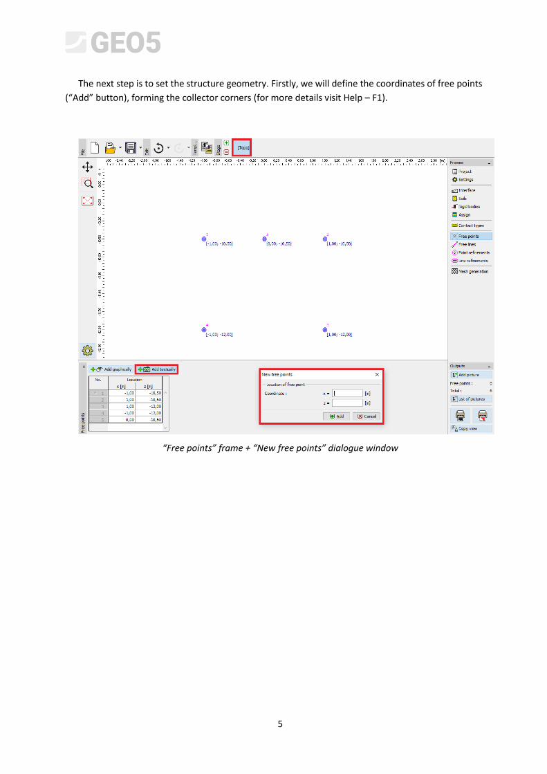
The next step is to set the structure geometry. Firstly, we will define the coordinates of free points

(“Add” button), forming the collector corners (for more details visit Help – F1).

“Free points” frame + “New free points” dialogue window

6

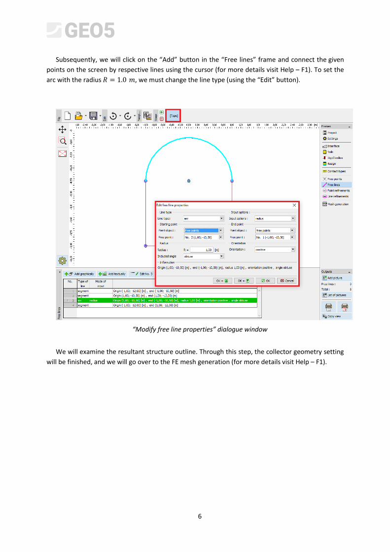
Subsequently, we will click on the “Add” button in the “Free lines” frame and connect the given

points on the screen by respective lines using the cursor (for more details visit Help – F1). To set the

arc with the radius 𝑅 = 1.0 𝑚, we must change the line type (using the “Edit” button).

“Modify free line properties” dialogue window

We will examine the resultant structure outline. Through this step, the collector geometry setting

will be finished, and we will go over to the FE mesh generation (for more details visit Help – F1).

7

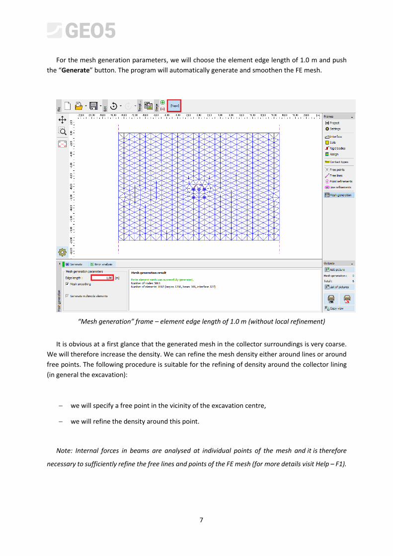
For the mesh generation parameters, we will choose the element edge length of 1.0 m and push

the “Generate” button. The program will automatically generate and smoothen the FE mesh.

“Mesh generation” frame – element edge length of 1.0 m (without local refinement)

It is obvious at a first glance that the generated mesh in the collector surroundings is very coarse.

We will therefore increase the density. We can refine the mesh density either around lines or around

free points. The following procedure is suitable for the refining of density around the collector lining

(in general the excavation):

− we will specify a free point in the vicinity of the excavation centre,

− we will refine the density around this point.

Note: Internal forces in beams are analysed at individual points of the mesh and it is therefore

necessary to sufficiently refine the free lines and points of the FE mesh (for more details visit Help – F1).

8

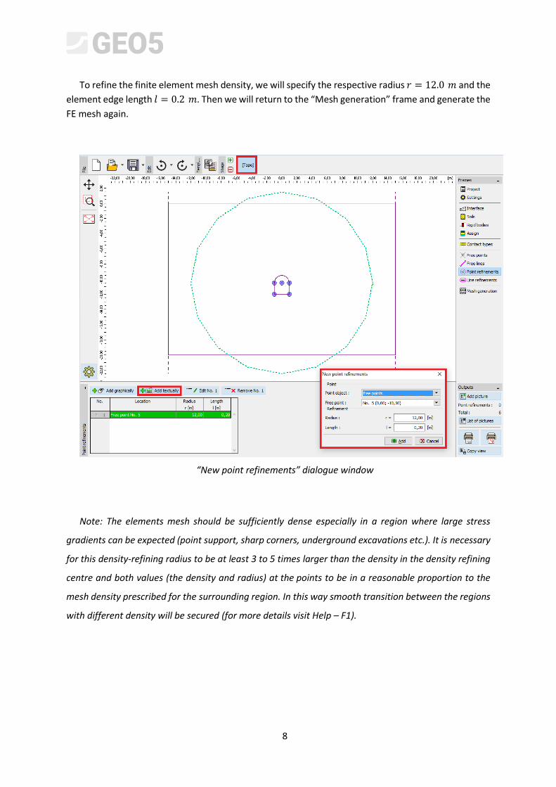
To refine the finite element mesh density, we will specify the respective radius 𝑟 = 12.0 𝑚 and the

element edge length 𝑙 = 0.2 𝑚. Then we will return to the “Mesh generation” frame and generate the

FE mesh again.

“New point refinements” dialogue window

Note: The elements mesh should be sufficiently dense especially in a region where large stress

gradients can be expected (point support, sharp corners, underground excavations etc.). It is necessary

for this density-refining radius to be at least 3 to 5 times larger than the density in the density refining

centre and both values (the density and radius) at the points to be in a reasonable proportion to the

mesh density prescribed for the surrounding region. In this way smooth transition between the regions

with different density will be secured (for more details visit Help – F1).

9

“Mesh generation” frame – FE edge length of 1.0 m (with locally increased mesh density in the

collector surrounding)

10

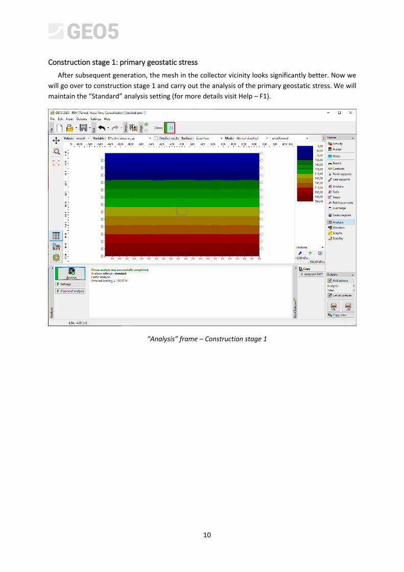
Construction stage 1: primary geostatic stress

After subsequent generation, the mesh in the collector vicinity looks significantly better. Now we

will go over to construction stage 1 and carry out the analysis of the primary geostatic stress. We will

maintain the “Standard” analysis setting (for more details visit Help – F1).

“Analysis” frame – Construction stage 1

11

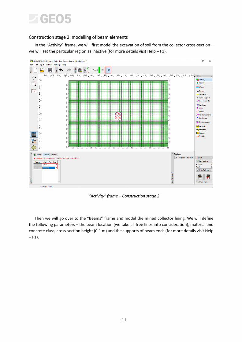
Construction stage 2: modelling of beam elements

In the “Activity” frame, we will first model the excavation of soil from the collector cross-section –

we will set the particular region as inactive (for more details visit Help – F1).

“Activity” frame – Construction stage 2

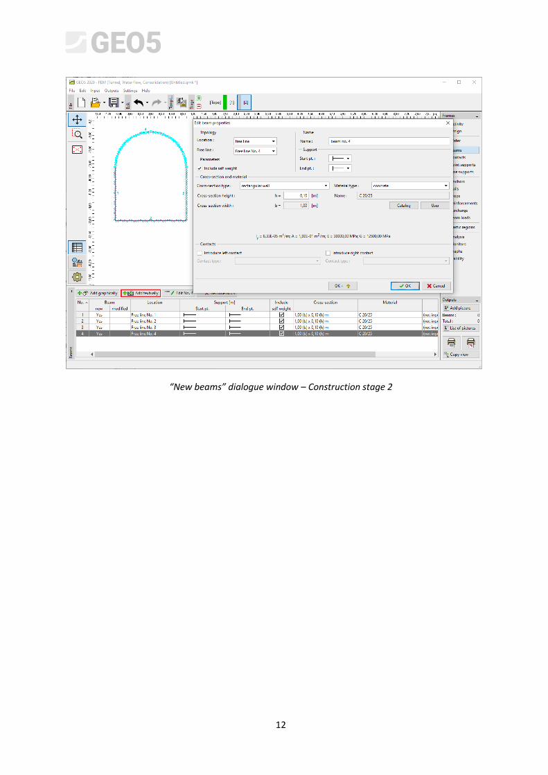
Then we will go over to the “Beams” frame and model the mined collector lining. We will define

the following parameters – the beam location (we take all free lines into consideration), material and

concrete class, cross-section height (0.1 m) and the supports of beam ends (for more details visit Help

– F1).

12

“New beams” dialogue window – Construction stage 2

13

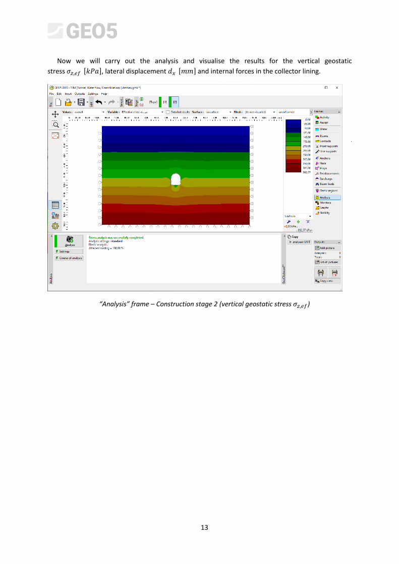
Now we will carry out the analysis and visualise the results for the vertical geostatic

stress 𝜎𝑧,𝑒𝑓 [𝑘𝑃𝑎], lateral displacement 𝑑𝑥 [𝑚𝑚] and internal forces in the collector lining.

“Analysis” frame – Construction stage 2 (vertical geostatic stress 𝜎𝑧,𝑒𝑓)

14

It follows from the picture that the maximum horizontal displacement is 2.2 mm (the collector

behaves as a rigid body). To better understand the structure behaviour, we will visualise the deformed

mesh (the button in the upper part of screen).

“Analysis” frame – Construction stage 2 (horizontal displacement 𝑑𝑥 after excavating the soil)

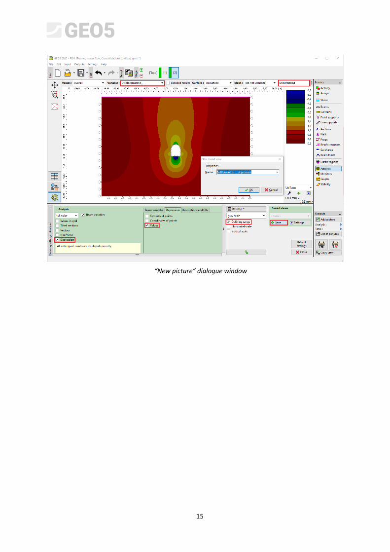
Note: Individual current views presented on the screen ca also be downloaded as independent

objects. They can also be managed afterwards. In this way the visualization of results is significantly

accelerated (for more details visit Help – F1).

15

“New picture” dialogue window

16

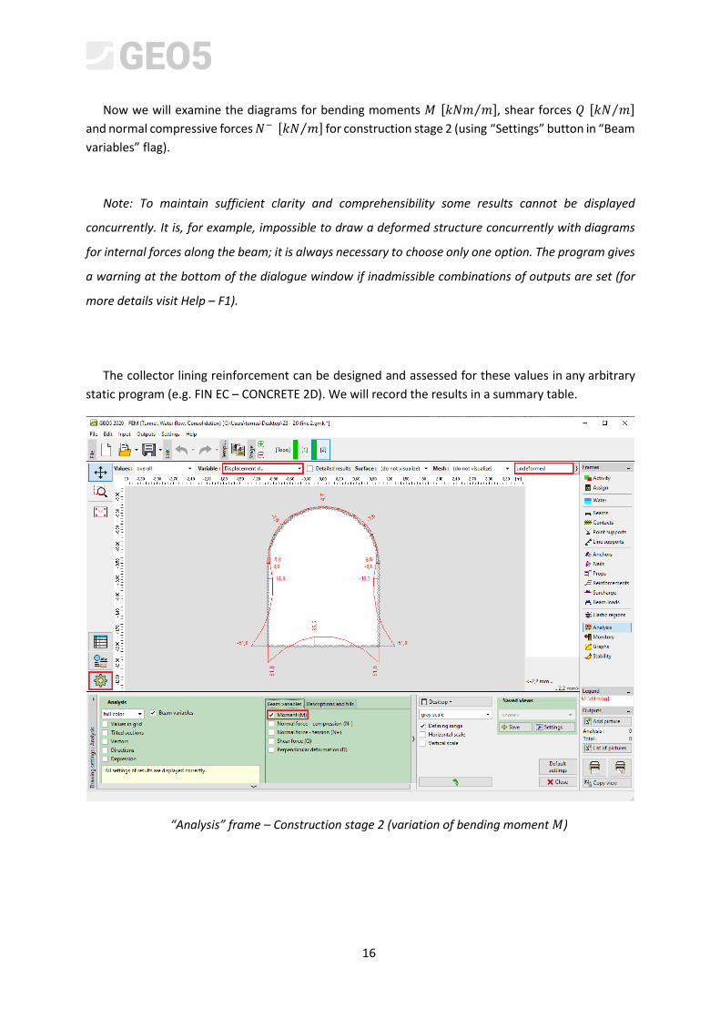
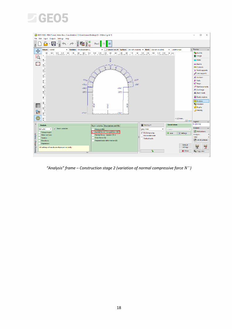
Now we will examine the diagrams for bending moments 𝑀 [𝑘𝑁𝑚 𝑚⁄ ], shear forces 𝑄 [𝑘𝑁 𝑚⁄ ]

and normal compressive forces 𝑁− [𝑘𝑁 𝑚⁄ ] for construction stage 2 (using “Settings” button in “Beam

variables” flag).

Note: To maintain sufficient clarity and comprehensibility some results cannot be displayed

concurrently. It is, for example, impossible to draw a deformed structure concurrently with diagrams

for internal forces along the beam; it is always necessary to choose only one option. The program gives

a warning at the bottom of the dialogue window if inadmissible combinations of outputs are set (for

more details visit Help – F1).

The collector lining reinforcement can be designed and assessed for these values in any arbitrary

static program (e.g. FIN EC – CONCRETE 2D). We will record the results in a summary table.

“Analysis” frame – Construction stage 2 (variation of bending moment 𝑀)

17

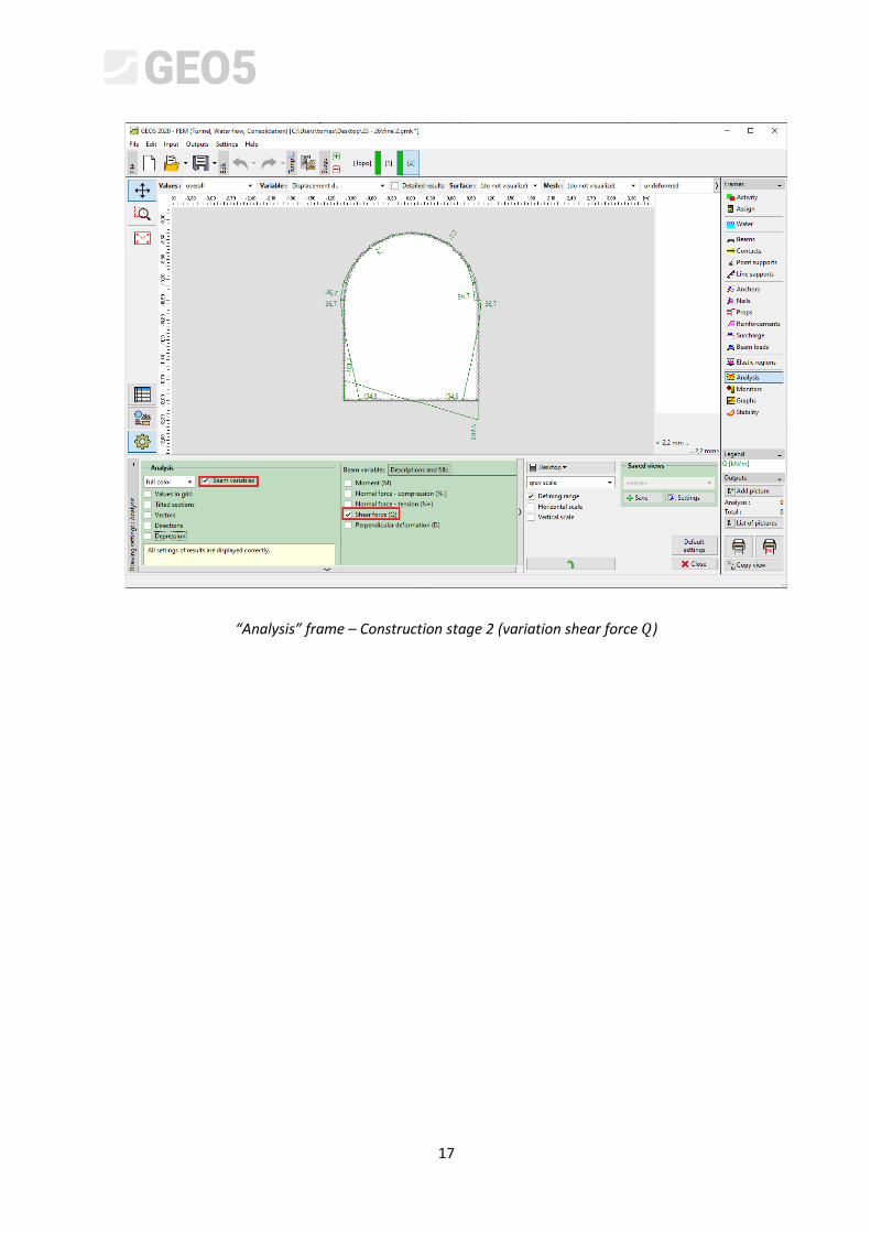
“Analysis” frame – Construction stage 2 (variation shear force 𝑄)

18

“Analysis” frame – Construction stage 2 (variation of normal compressive force 𝑁−)

19

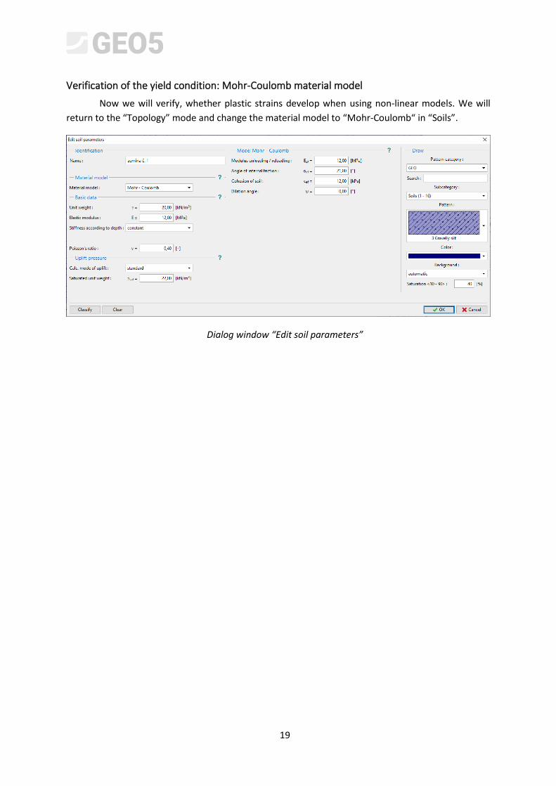
Verification of the yield condition: Mohr-Coulomb material model

Now we will verify, whether plastic strains develop when using non-linear models. We will

return to the “Topology” mode and change the material model to “Mohr-Coulomb“ in “Soils”.

Dialog window “Edit soil parameters”

20

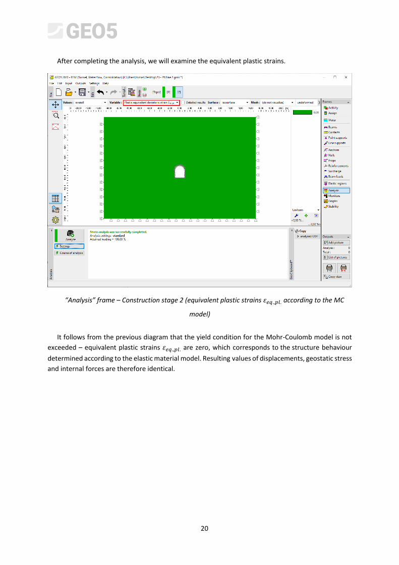
After completing the analysis, we will examine the equivalent plastic strains.

“Analysis” frame – Construction stage 2 (equivalent plastic strains 𝜀𝑒𝑞.,𝑝𝑙. according to the MC

model)

It follows from the previous diagram that the yield condition for the Mohr-Coulomb model is not

exceeded – equivalent plastic strains 𝜀𝑒𝑞.,𝑝𝑙. are zero, which corresponds to the structure behaviour

determined according to the elastic material model. Resulting values of displacements, geostatic stress

and internal forces are therefore identical.

21

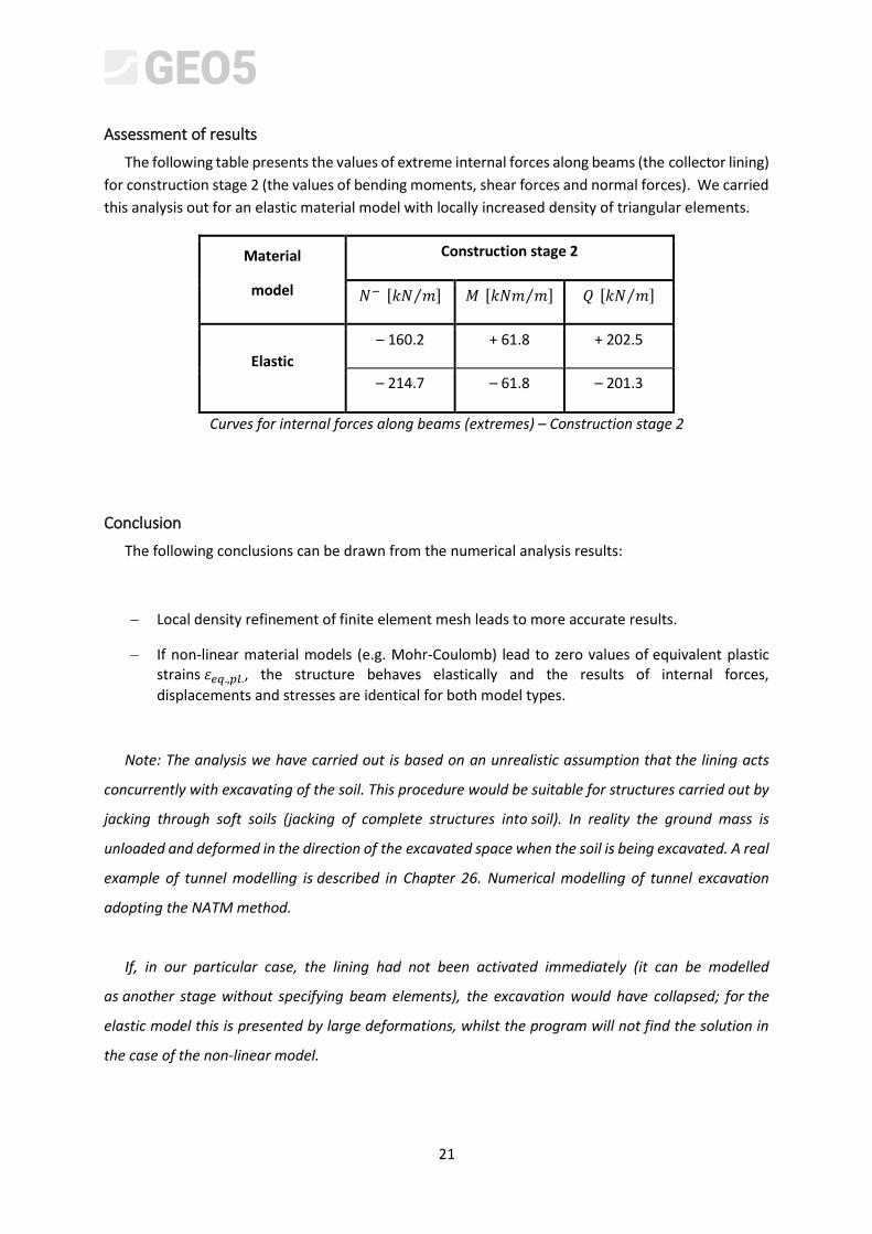
Assessment of results

The following table presents the values of extreme internal forces along beams (the collector lining)

for construction stage 2 (the values of bending moments, shear forces and normal forces). We carried

this analysis out for an elastic material model with locally increased density of triangular elements.

Material

model

Construction stage 2

𝑁− [𝑘𝑁 𝑚⁄ ] 𝑀 [𝑘𝑁𝑚 𝑚⁄ ] 𝑄 [𝑘𝑁 𝑚⁄ ]

Elastic

– 160.2 + 61.8 + 202.5

– 214.7 – 61.8 – 201.3

Curves for internal forces along beams (extremes) – Construction stage 2

Conclusion

The following conclusions can be drawn from the numerical analysis results:

− Local density refinement of finite element mesh leads to more accurate results.

− If non-linear material models (e.g. Mohr-Coulomb) lead to zero values of equivalent plastic strains 𝜀𝑒𝑞.,𝑝𝑙., the structure behaves elastically and the results of internal forces,

displacements and stresses are identical for both model types.

Note: The analysis we have carried out is based on an unrealistic assumption that the lining acts

concurrently with excavating of the soil. This procedure would be suitable for structures carried out by

jacking through soft soils (jacking of complete structures into soil). In reality the ground mass is

unloaded and deformed in the direction of the excavated space when the soil is being excavated. A real

example of tunnel modelling is described in Chapter 26. Numerical modelling of tunnel excavation

adopting the NATM method.

If, in our particular case, the lining had not been activated immediately (it can be modelled

as another stage without specifying beam elements), the excavation would have collapsed; for the

elastic model this is presented by large deformations, whilst the program will not find the solution in

the case of the non-linear model.

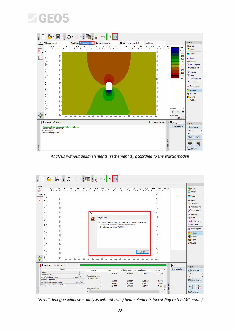
22

Analysis without beam elements (settlement 𝑑𝑧 according to the elastic model)

“Error” dialogue window – analysis without using beam elements (according to the MC model)