Embed Size (px)
Citation preview
THE JOURNAL OF FINANCE • VOL. LXIII, NO. 5 • OCTOBER 2008
Collective Risk Management in a Flightto Quality Episode
RICARDO J. CABALLERO and ARVIND KRISHNAMURTHY∗
ABSTRACT
Severe flight to quality episodes involve uncertainty about the environment, not onlyrisk about asset payoffs. The uncertainty is triggered by unusual events and untestedfinancial innovations that lead agents to question their worldview. We present a modelof crises and central bank policy that incorporates Knightian uncertainty. The modelexplains crisis regularities such as market-wide capital immobility, agents’ disen-gagement from risk, and liquidity hoarding. We identify a social cost of these behav-iors, and a benefit of a lender of last resort facility. The benefit is particularly highbecause public and private insurance are complements during uncertainty-drivencrises.
Policy practitioners operating under a risk-management para-digm may, at times, be led to undertake actions intended to provide in-surance against especially adverse outcomes. . . When confronted withuncertainty, especially Knightian uncertainty, human beings invariablyattempt to disengage from medium to long-term commitments in favor ofsafety and liquidity. . . The immediate response on the part of the centralbank to such financial implosions must be to inject large quantities ofliquidity. . .” Alan Greenspan (2004).
FLIGHT TO QUALITY EPISODES ARE AN IMPORTANT SOURCE of financial and macroeco-nomic instability. Modern examples of these episodes in the U.S. include thePenn Central default of 1970, the stock market crash of 1987, the events in thefall of 1998 beginning with the Russian default and ending with the bailoutof LTCM, and the events that followed the attacks of 9/11. Behind each of
∗Caballero is from MIT and NBER. Krishnamurthy is from Northwestern University and NBER.We are grateful to Marios Angeletos, Olivier Blanchard, Phil Bond, Craig Burnside, Jon Faust,Xavier Gabaix, Jordi Gali, Michael Golosov, Campbell Harvey, William Hawkins, Burton Holli-field, Bengt Holmstrom, Urban Jermann, Dimitri Vayanos, Ivan Werning, an associate editor andanonymous referee, as well as seminar participants at Atlanta Fed Conference on Systematic Risk,Bank of England, Central Bank of Chile, Columbia, DePaul, Imperial College, London BusinessSchool, London School of Economics, Northwestern, MIT, Wharton, NY Fed Liquidity Conference,NY Fed Money Markets Conference, NBER Economic Fluctuations and Growth meeting, NBERMacroeconomics and Individual Decision Making Conference, Philadelphia Fed, and Universityof British Columbia Summer Conference for their comments. Vineet Bhagwat, David Lucca, andAlp Simsek provided excellent research assistance. Caballero thanks the NSF for financial sup-port. This paper covers the same substantive issues as (and hence replaces) “Flight to Quality andCollective Risk Management,” NBER WP # 12136.
2195
2196 The Journal of Finance
these episodes lies the specter of a meltdown that may lead to a prolongedslowdown as in Japan during the 1990s, or even a catastrophe like the GreatDepression.1 In each of these cases, as hinted at by Greenspan (2004), the Fedintervened early and stood ready to intervene as much as needed to prevent ameltdown.
In this paper we present a model to study the benefits of central bank actionsduring flight to quality episodes. Our model has two key ingredients: capi-tal/liquidity shortages and Knightian uncertainty (Knight (1921)). The capitalshortage ingredient is a recurring theme in the empirical and theoretical liter-ature on financial crises and requires little motivation. Knightian uncertaintyis less commonly studied, but practitioners perceive it as a central ingredientto flight to quality episodes (see Greenspan’s quote).
Most flight to quality episodes are triggered by unusual or unexpected events.In 1970, the Penn Central Railroad’s default on prime-rated commercial papercaught the market by surprise and forced investors to reevaluate their modelsof credit risk. The ensuing dynamics temporarily shut out a large segment ofcommercial paper borrowers from a vital source of funds. In October 1987, thespeed of the stock market decline took investors and market makers by sur-prise, causing them to question their models. Investors pulled back from themarket while key market-makers widened bid-ask spreads. In the fall of 1998,the comovement of Russian government bond spreads, Brazilian spreads, andU.S. Treasury bond spreads was a surprise to even sophisticated market par-ticipants. These high correlations rendered standard risk management mod-els obsolete, leaving financial market participants searching for new models.Agents responded by making decisions using “worst-case” scenarios and “stress-testing” models. Finally, after 9/11, regulators were concerned that commercialbanks would respond to the increased uncertainty over the status of other com-mercial banks by individually hoarding liquidity and that such actions wouldlead to gridlock in the payments system.2
The common aspects of investor behavior across these episodes—re-evaluation of models, conservatism, and disengagement from risky activities—indicate that these episodes involved Knightian uncertainty (i.e., immeasurablerisk) and not merely an increase in risk exposure. The emphasis on tail out-comes and worst-case scenarios in agents’ decision rules suggests uncertaintyaversion. Finally, an important observation about these events is that when itcomes to flight to quality episodes, history seldom repeats itself. Similar mag-nitudes of commercial paper default (Mercury Finance in 1997) or stock marketpullbacks (mini-crash of 1989) did not lead to similar investor responses. Today,as opposed to in 1998, market participants understand that correlations shouldbe expected to rise during periods of reduced liquidity. Creditors understandthe risk involved in lending to hedge funds. While in 1998 hedge funds were still
1 See table 1 (part A) in Barro (2006) for a list of extreme events, measured in terms of declinein GDP, in developed economies during the 20th century.
2 See Calomiris (1994) on the Penn Central default, Melamed (1998) on the 1987 market crash,Scholes (2000) on the events of 1998, and Stewart (2002) or McAndrews and Potter (2002) on 9/11.
Collective Risk Management in a Flight to Quality Episode 2197
a novel financial vehicle, the large reported losses of the Amaranth hedge fundin 2006 barely caused a ripple in financial markets. The one-of-a-kind aspect offlight to quality episodes suggests that these events are fundamentally aboutuncertainty rather than risk.3
Section I of the paper lays out a model of financial crises based on liquidityshortages and Knightian uncertainty. We analyze the model’s equilibrium andshow that an increase in Knightian uncertainty or decrease in aggregate liquid-ity can generate flight to quality effects. In the model, when an agent is facedwith Knightian uncertainty, he considers the worst case among the scenariosover which he is uncertain. This modeling of agent decision making and Knight-ian uncertainty draws from the decision theory literature, and in particularfrom Gilboa and Schmeidler (1989). When the aggregate quantity of liquidityis limited, the Knightian agent grows concerned that he will be caught in a sit-uation in which he needs liquidity, but there is not enough liquidity available tohim. In this context, agents react by shedding risky financial claims in favor ofsafe and uncontingent claims. Financial intermediaries become self-protectiveand hoard liquidity. Investment banks and trading desks turn conservative intheir allocation of risk capital. They lock up capital and become unwilling toflexibly move it across markets.
The main results of our paper are in Sections II and III. As indicated by for-mer Federal Reserve Chairman Greenspan’s comments, the Fed has historicallyintervened during flight to quality episodes. We analyze the macroeconomicproperties of the equilibrium and study the effects of central bank actions inour environment. First, we show that Knightian uncertainty leads to a collectivebias in agents’ actions: Each agent covers himself against his own worst-casescenario, but the scenario that the collective of agents are guarding againstis impossible, and known to be so despite agents’ uncertainty about the envi-ronment. We show that agents’ conservative actions such as liquidity hoardingand locking-up of capital are macroeconomically costly because scarce liquiditygoes wasted. Second, we show that central bank policy can be designed to alle-viate the overconservatism. A lender of last resort (LLR), even one facing thesame incomplete knowledge that triggers agents’ Knightian responses, findsthat committing to add liquidity in the unlikely event that the private sector’sliquidity is depleted is beneficial. Agents respond to the LLR by freeing upcapital and altering decisions in a manner that wastes less private liquidity.Public and private provision of insurance are complements in our model: Eachpledged dollar of public intervention in the extreme event is matched by a com-parable private sector reaction to free up capital. In this sense, the Fed’s LTCMrestructuring was important not for its direct effect, but because it served asa signal of the Fed’s readiness to intervene should conditions worsen. We alsoshow that the LLR must be a last-resort policy: If liquidity injections take place
3 This observation suggests a possible way to empirically disentangle uncertainty aversion fromrisk aversion or extreme forms of risk aversion such as negative skew aversion. A risk averse agentbehaves conservatively during times of high risk—it does not matter whether the risk involvessomething new or not. For an uncertainty-averse agent, new forms of risk elicit the conservativereaction.
2198 The Journal of Finance
too often, the policy exacerbates the private sector’s mistakes and reduces thevalue of intervention. This occurs for reasons akin to the moral hazard problemidentified with the LLR.
Our model is most closely related to the literature on banking crises initiatedby Diamond and Dybvig (1983).4 While our environment is a variant of that inDiamond and Dybvig, it does not include the sequential service constraint ofDiamond and Dybvig, and instead emphasizes Knightian uncertainty. The mod-eling difference leads to different applications of our crisis model. For instance,our model applies to a wider set of financial intermediaries than commercialbanks financed by demandable deposit contracts. More importantly, becauseour model of crises centers on Knightian uncertainty, its insights most directlyapply to circumstances of market-wide uncertainty, such as the new financialinnovations or events discussed above.
At a theoretical level, the sequential service constraint in the Diamond andDybvig model creates a coordination failure. The bank “panic” occurs becauseeach depositor runs conjecturing that other depositors will run. The externalityin the depositor’s run decisions is central to their model of crises.5 In our model,it is an increase in Knightian uncertainty that generates the panic behavior. Ofcourse, in reality crises may reflect both the type of externalities that Diamondand Dybvig highlight and the uncertainties that we study. In the Diamond andDybvig analysis, the LLR is always beneficial because it rules out the “bad” runequilibrium caused by the coordination failure.6 As noted above, our model’sprescriptions center on situations of market-wide uncertainty. In particular,our model prescribes that the benefit of the LLR is highest when there is bothinsufficient aggregate liquidity and Knightian uncertainty.
Holmstrom and Tirole (1998) study how a shortage of aggregate collaterallimits private liquidity provision (see also Woodford (1990)). Their analysissuggests that a credible government can issue government bonds that can thenbe used by the private sector for liquidity provision. The key difference betweenour paper and those of Holmstrom and Tirole and Woodford is that we showaggregate collateral may be inefficiently used, so that private sector liquidityprovision is limited. In our model, government intervention not only adds tothe private sector’s collateral, but also, and more centrally, improves the use ofprivate collateral.
4 The literature on banking crises is too large to discuss here. See Gorton and Winton (2003) fora survey of this literature.
5 More generally, other papers in the crisis literature also highlight how investment externalitiescan exacerbate crises. Some examples in this literature include Allen and Gale (1994), Gromb andVayanos (2002), Caballero and Krishnamurthy (2003), or Rochet and Vives (2004). In many of thesemodels, incomplete markets lead to an inefficiency that creates a role for central bank policy (seeRochet and Vives (2004) or Allen and Gale (2004)).
6 More generally, other papers in the crisis literature also highlight how investment externalitiescan exacerbate crises. Some examples in this literature include Allen and Gale (1994), Gromb andVayanos (2002), Caballero and Krishnamurthy (2003), or Rochet and Vives (2004). In many of thesemodels, incomplete markets leads to an inefficiency that creates a role for central bank policy (seeBhattacharya and Gale (1987), Rochet and Vives (2004) or Allen and Gale (2004)).
Collective Risk Management in a Flight to Quality Episode 2199
Routledge and Zin (2004) and Easley and O’Hara (2005) are two related anal-yses of Knightian uncertainty in financial markets.7 Routledge and Zin beginfrom the observation that financial institutions follow decision rules to pro-tect against a worst case scenario. They develop a model of market liquidityin which an uncertainty averse market maker sets bids and asks to facilitatetrade of an asset. Their model captures an important aspect of flight to quality,namely, that uncertainty aversion can lead to a sudden widening of the bid-askspread, causing agents to halt trading and reducing market liquidity. Both ourpaper and Routledge and Zin share the emphasis on financial intermediationand uncertainty aversion as central ingredients in flight to quality episodes.However, each paper captures different aspects of flight to quality. Easley andO’Hara (2005) study a model in which uncertainty-averse traders focus on aworst-case scenario when making an investment decision. Like us, Easley andO’Hara point out that government intervention in a worst-case scenario canhave large effects. Easley and O’Hara study how uncertainty aversion affectsinvestor participation in stock markets, while the focus of our study is on un-certainty aversion and financial crises.
I. The Model
We study a model conditional on entering a turmoil period in which liquidityrisk and Knightian uncertainty coexist. Our model is silent on what triggers theepisode. In practice, we think that the occurrence of an unusual event, such asthe Penn Central default or the losses on AAA-rated subprime mortgage-backedsecurities, causes agents to reevaluate their models and triggers robustnessconcerns. Our goal is to present a model to study the role of a centralized liq-uidity provider such as the central bank.
A. The Environment
A.1. Preferences and Shocks
The model has a continuum of competitive agents, which are indexed byω ∈ � ≡ [0, 1]. An agent may receive a liquidity shock in which he needs someliquidity immediately. We view these liquidity shocks as a parable for a suddenneed for capital by a financial market specialist (e.g., a trading desk, hedgefund, market maker).
The shocks are correlated across agents. With probability φ (1), the economyis hit by a first wave of liquidity shocks. In this wave, a randomly chosen groupof one-half of the agents have liquidity needs. We denote by φω(1) the probability
7 A growing economics literature aims to formalize Knightian uncertainty (a partial list of contri-butions includes Gilboa and Schmeidler (1989), Dow and Werlang (1992), Epstein and Wang (1994),Hansen and Sargent (1995, 2003), Skiadas (2003), Epstein and Schneider (2004), and Hansen(2006)). As in much of this literature, we use a max-min device to describe agents’ expected utility.Our treatment of Knightian uncertainty is most similar to Gilboa and Schmeidler, in that agentschoose a worst case among a class of priors.
2200 The Journal of Finance
of agent ω receiving a shock in the first wave, and note that,∫�
φω(1) dω = φ(1)2
. (1)
Equation (1) states that on average, across all agents, the probability of anagent receiving a shock in the first wave is φ(1)
2 .With probability φ(2|1), a second wave of liquidity shocks hits the economy. In
the second wave of liquidity shocks, the other half of the agents need liquidity.Let φ(2) = φ(1)φ(2|1). The probability with which agent ω is in this second waveis φω(2), which satisfies ∫
�
φω(2) dω = φ(2)2
. (2)
With probability 1 − φ(1) > 0 the economy experiences no liquidity shocks.We note that the sequential shock structure means that
φ(1) > φ(2) > 0. (3)
This condition states that, in aggregate, a single-wave event is more likelythan the two-wave event. We refer to the two-wave event as an extreme event,capturing an unlikely but severe liquidity crisis in which many agents areaffected. Relation (3), which derives from the sequential shock structure, playsan important role in our analysis.
We model the liquidity shock as a shock to preferences (e.g., as in Diamondand Dybvig (1983)). Agent ω receives utility
Uω(c1, c2, cT ) = α1u(c1) + α2u(c2) + βcT . (4)
We define α1 = 1, α2 = 0 if the agent is in the early wave; α1 = 0, α2 = 1 if theagent is in the second wave; and, α1 = 0, α2 = 0 if the agent is not hit by a shock.We will refer to the first shock date as “date 1,” the second shock date as “date2,” and the final date as “date T.”
The function u : R+ → R is twice continuously differentiable, increasing, andstrictly concave, and it satisfies the condition limc→0u′(c) = ∞. Preferences areconcave over c1 and c2, and linear over cT. We view the preference over cT ascapturing a time in the future when market conditions are normalized andthe trader is effectively risk neutral. The concave preferences over c1 and c2reflect the potentially higher marginal value of liquidity during a time of marketdistress. The discount factor, β, can be thought of as an interest rate ( 1
β− 1)
facing the trader.
A.2. Endowment and Securities
Each agent is endowed with Z units of goods. These goods can be stored atgross return of one, and then liquidated if an agent receives a liquidity shock.If we interpret the agents of the model as financial traders, we may think of Zas the capital or liquidity of a trader.
Collective Risk Management in a Flight to Quality Episode 2201
Agents can also trade financial claims that are contingent on shock realiza-tions. As we will show, these claims allow agents who do not receive a shock toinsure agents who do receive a shock.
We assume all shocks are observable and contractible. There is no concernthat an agent will pretend to have a shock and collect on an insurance claim.Markets are complete. There are claims on all histories of shock realizations.We will be more precise in specifying these contingent claims when we analyzethe equilibrium.
A.3. Probabilities and Uncertainty
Agents trade contingent claims to insure against their liquidity shocks. Inmaking the insurance decisions, agents have a probability model of the liquidityshocks in mind.
We assume that agents know the aggregate shock probabilities, φ(1) and φ(2).We may think that agents observe the past behavior of the economy and formprecise estimates of these aggregate probabilities. However, centrally to ourmodel, the same past data do not reveal whether a given ω is more likely tobe in the first wave or the second wave. Agents treat the latter uncertainty asKnightian.
Formally, we use φω(1) to denote the true probability of agent ω receivingthe first shock, and φω
ω (1) to denote agent ω’s perception of the relevant trueprobability (similarly for φω(2) and φω
ω (2)). We assume that each agent ω knowshis probability of receiving a shock either in the first or second wave, φω(1) +φω(2), and thus the perceived probabilities satisfy8
φωω (1) + φω
ω (2) = φω(1) + φω(2) = φ(1) + φ(2)2
. (5)
We define
θωω ≡ φω
ω (2) − φ(2)2
. (6)
That is, θωω reflects how much agent ω’s probability assessment of being second
is higher than the average agent in the economy’s true probability of beingsecond. This relation also implies that
−θωω = φω
ω (1) − φ(1)2
.
Agents consider a range of probability models θωω in the set , with support
[−K, +K ](K < φ(2)/2), and design insurance portfolios that are robust to theirmodel uncertainty. We follow Gilboa and Schmeidler’s (1989) Maximin Expected
8 For further clarification of the structure of shocks and agents’ uncertainty, see the event treethat is detailed in the Appendix.
2202 The Journal of Finance
Utility representation of Knightian uncertainty aversion and write
max(c1,c2,cT )
minθωω ∈
E0[Uω(c1, c2, cT )|θωω ], (7)
where K captures the extent of agents’ uncertainty.In a flight to quality, such as during the fall of 1998 or 9/11, agents are
concerned about systemic risk and unsure of how this risk will impinge ontheir activities. They may have a good understanding of their own markets,but be unsure of how the behavior of agents in other markets may affect them.For example, during 9/11 market participants feared gridlock in the paymentssystem. Each participant knew how much he owed to others but was unsurewhether resources owed to him would arrive (see, for example, Stewart (2002)or McAndrews and Potter (2002)). In our model, agents are certain about theprobability of receiving a shock, but are uncertain about the probability withwhich their shocks will occur early or late relative to others.
We view agents’ max-min preferences in (7) as descriptive of their decisionrules. The widespread use of worst-case scenario analysis in decision makingby financial firms is an example of the robustness preferences of such agents.
It is also important to note that the objective function in (7) works throughaltering the probability distribution used by agents. That is, given an agent’suncertainty, the min operator in (7) has the agent making decisions using theworst-case probability distribution over this uncertainty. This objective is differ-ent from one that asymmetrically penalizes bad outcomes. That is, a loss aver-sion or negative skewness aversion objective function leads an agent to worryabout worst cases through the utility function Uω directly. This asymmetric util-ity function model predicts that agents always worry about the downside. OurKnightian uncertainty objective predicts that agents worry about the downsidein particular during times of model uncertainty. As discussed in the introduc-tion, it appears that flight to quality episodes have a “newness/uncertainty”element, which our model can capture.
The distinction is also relevant because probabilities have to satisfy addingup constraints across all agents, that is,
∫�
θωdω = 0. Indeed, we use the term“collective” bias to refer to a situation where agents’ individual probability dis-tributions from the min operator in (7) fail to satisfy an adding-up constraint.As we will explain below, the efficiency results we present later in the paperstem from this aspect of our model.
A.4. Symmetry
To simplify our analysis we assume that the agents are symmetric at date0. While each agent’s true θω may be different, the θω for every agent is drawnfrom the same .
The symmetry applies in other dimensions as well: φω, K, Z, and u(c) arethe same for all ω. Moreover, this information is common knowledge. As notedabove, φ(1) and φ(2) are also common knowledge.
Collective Risk Management in a Flight to Quality Episode 2203
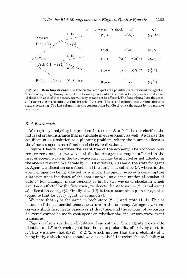
Figure 1. Benchmark case. The tree on the left depicts the possible states realized for agent ω.The economy can go through zero (lower branch), one (middle branch), or two (upper branch) wavesof shocks. In each of these cases, agent ω may or may not be affected. The first column lists the state,s, for agent ω corresponding to that branch of the tree. The second column lists the probability ofstate s occurring. The last column lists the consumption bundle given to the agent by the plannerin state s.
B. A Benchmark
We begin by analyzing the problem for the case K = 0. This case clarifies thenature of cross-insurance that is valuable in our economy as well. We derive theequilibrium as a solution to a planning problem, where the planner allocatesthe Z across agents as a function of shock realizations.
Figure 1 below describes the event tree of the economy. The economy mayreceive zero, one, or two waves of shocks. An agent ω may be affected in thefirst or second wave in the two-wave case, or may be affected or not affected inthe one-wave event. We denote by s = ( # of waves, ω’s shock) the state for agentω. Agent ω’s allocation as a function of the state is denoted by Cs, where, in theevent of agent ω being affected by a shock, the agent receives a consumptionallocation upon incidence of the shock as well as a consumption allocation atdate T. For example, if the economy is hit by two waves of shocks in whichagent ω is affected by the first wave, we denote the state as s = (2, 1) and agentω’s allocation as (c1, cs
T). Finally, C = {Cs} is the consumption plan for agent ω
(equal to that for every agent, by symmetry).We note that c1 is the same in both state (2, 1) and state (1, 1). This is
because of the sequential shock structure in the economy. An agent who re-ceives a shock first needs resources at that time, and the amount of resourcesdelivered cannot be made contingent on whether the one- or two-wave eventtranspires.
Figure 1 also gives the probabilities of each state s. Since agents are ex anteidentical and K = 0, each agent has the same probability of arriving at states. Thus we know that φω(2) = φ(2)/2, which implies that the probability of ω
being hit by a shock in the second wave is one-half. Likewise, the probability of
2204 The Journal of Finance
ω being hit by a shock in the first wave is one-half. These computations lead tothe probabilities given in Figure 1.
The planner’s problem is to solve
maxC
∑psUω(Cs)
subject to resource constraints that, for every shock realization, the promisedconsumption amounts are not more than the total endowment of Z, that is,
c0,no ≤ Z12
(c1 + c1,1
T + c1,noT
) ≤ Z12
(c1 + c2,1
T + c2 + c2,2T
) ≤ Z ,
as well as nonnegativity constraints that, for each s, every consumption amountin Cs is nonnegative.
It is obvious that if shocks do not occur, then the planner will give Z to eachof the agents for consumption at date T. Thus c0,no
T = Z and we can drop thisconstant from the objective. We rewrite the problem as
maxC
φ(1) − φ(2)2
(u(c1) + βc1,1
T + βc1,noT
) + φ(2)2
(u(c1) + u(c2) + βc2,1
T + βc2,2T
)subject to resource and nonnegativity constraints.
Observe that c1,1T and c1,no
T enter as a sum in both the objective and the con-straints. Without loss of generality we set c1,1
T = 0 . Likewise, c2,1T and c2,2
T enteras a sum in both the objective and the constraints. Without loss of generalitywe set c2,1
T = 0. The reduced problem is:
max(c1,c2,c1,no
T ,c2,2T )
φ(1)u(c1) + φ(2)(u(c2) + βc2,2
T
) + (φ(1) − φ(2)
)βc1,no
T
subject to
c1 + c1,noT = 2Z
c1 + c2 + c2,2T = 2Z
c1, c2, c1,noT , c2,2
T ≥ 0.
Note that the resource constraints must bind. The solution hinges on whetherthe nonnegativity constraints on consumption bind or not.
If the nonnegativity constraints do not bind, then the first-order conditionsfor c1 and c2 yield
c1 = c2 = u′−1(β) ≡ c∗.
The solution implies that
c2,2T = 2(Z − c∗), c1,no
T = 2Z − c∗.
Collective Risk Management in a Flight to Quality Episode 2205
Thus, the nonnegativity constraints do not bind if Z ≥ c∗. We refer to this caseas one of sufficient aggregate liquidity. When Z is large enough, agents are ableto finance a consumption plan in which marginal utility is equalized acrossall states. At the optimum, agents equate the marginal utility of early con-sumption with that of date T consumption, which is β given the linear utilityover cT. A low value of β means that agents discount the future heavily andrequire more early consumption. Loosely speaking we can think of this caseas one where an agent is “constrained” and places a high value on currentliquidity. As a result, the economy needs more liquidity (Z) to satisfy agents’needs.
Now consider the case in which there is insufficient liquidity so that agentsare not able to achieve full insurance. This is the case where Z < c∗. It is obviousthat c2,2
T = 0 in this case (i.e., the planner uses all of the limited liquidity towardsshock states). Thus, for a given c1 we have that c2 = c1,no
T = 2Z − c1 and theproblem is
maxc1
φ(1)u(c1) + φ(2)u(2Z − c1) + (φ(1) − φ(2))β(2Z − c1) (8)
with first-order condition
u′(c1) = φ(2)φ(1)
u′(2Z − c1) + β
(1 − φ(2)
φ(1)
). (9)
Since u′(2Z − c1) > β (i.e., c2 < c∗) we can order
β < u′(c1) < u′(2Z − c1) ⇒ c1 > Z . (10)
The last inequality on the right of (10) is the important result from the anal-ysis. Agents who are affected by the first wave of shocks receive more liquiditythan agents who are affected by the second wave. There is cross-insurance be-tween agents. Intuitively, this is because the probability of the second waveoccurring is strictly smaller than that of the first wave (or, equivalently, condi-tional on the first wave having taken place there is a chance the economy willbe spared a second wave). Thus, when liquidity is scarce (small Z) it is optimalto allocate more of the limited liquidity to the more likely shock. On the otherhand, when liquidity is plentiful (large Z) the liquidity allocation of each agentis not contingent on the order of the shocks. This is because there is enoughliquidity to cover all shocks.
We summarize these results as follows:
PROPOSITION 1: The equilibrium in the benchmark economy with K = 0 has twocases:
(1) The economy has insufficient aggregate liquidity if Z < c∗. In this case,
c∗ > c1 > Z > c2.
Agents are partially insured against liquidity shocks. First-wave liquidityshocks are more insured than second-wave liquidity shocks.
2206 The Journal of Finance
(2) The economy has sufficient aggregate liquidity if Z ≥ c∗. In this case,
c1 = c2 = c∗
and agents are fully insured against liquidity shocks.
Flight to quality effects, and a role for central bank intervention, arise onlyin the first case (insufficient aggregate liquidity). This is the case we analyzein detail in the next sections.
C. Implementation
There are two natural implementations of the equilibrium: financial inter-mediation, and trading in shock-contingent claims.
In the intermediation implementation, each agent deposits Z in an interme-diary initially and receives the right to withdraw c1 > Z if he receives a shockin the first wave. Since shocks are fully observable, the withdrawal can be con-ditioned on the agents’ shocks. Agents who do not receive a shock in the firstwave own claims to the rest of the intermediary’s assets (Z − c1 < c1). The sec-ond group of agents either redeem their claims upon incidence of the secondwave of shocks, or at date T. Finally, if no shocks occur, the intermediary isliquidated at date T and all agents receive Z.
In the contingent claims implementation, each agent purchases a claim thatpays 2(c1 − Z) > 0 in the event that the agent receives a shock in the first wave.The agent sells an identical claim to every other agent, paying 2(c1 − Z) in caseof the first-wave shock. Note that this is a zero-cost strategy since both claimsmust have the same price.
If no shocks occur, agents consume their own Z. If an agent receives a shockin the first wave, he receives 2(c1 − Z) and pays out c1 − Z (since one-half ofthe agents are affected in the first wave), to net c1 − Z. Added to his initialliquidity endowment of Z, he has total liquidity of c1. Any later agent has Z −(c1 − Z) = 2Z − c1 units of liquidity to either finance a second shock, or date Tconsumption.
Finally, note that if there is sufficient aggregate liquidity either the interme-diation or contingent claims implementation achieves the optimal allocation.Moreover, in this case, the allocation is also implementable by self-insurance.Each agent keeps his Z and liquidates c∗ < Z to finance a shock. The self-insurance implementation is not possible when Z < c∗, because the allocationrequires each agent to receive more than his endowment of Z if the agent is hitfirst.
D. K > 0 Robustness Case
We now turn to the general problem, K > 0. Once again, we derive the equi-librium by solving a planning problem where the planner allocates the Z toagents as a function of shocks. When K > 0, agents make decisions based on
Collective Risk Management in a Flight to Quality Episode 2207
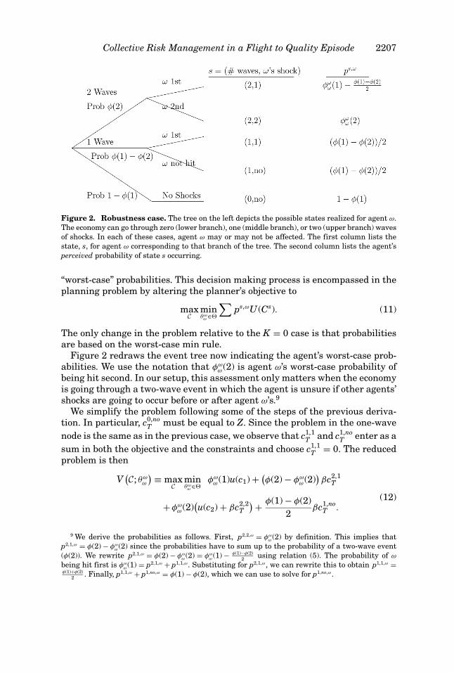
Figure 2. Robustness case. The tree on the left depicts the possible states realized for agent ω.The economy can go through zero (lower branch), one (middle branch), or two (upper branch) wavesof shocks. In each of these cases, agent ω may or may not be affected. The first column lists thestate, s, for agent ω corresponding to that branch of the tree. The second column lists the agent’sperceived probability of state s occurring.
“worst-case” probabilities. This decision making process is encompassed in theplanning problem by altering the planner’s objective to
maxC
minθωω ∈
∑ps,ωU (Cs). (11)
The only change in the problem relative to the K = 0 case is that probabilitiesare based on the worst-case min rule.
Figure 2 redraws the event tree now indicating the agent’s worst-case prob-abilities. We use the notation that φω
ω (2) is agent ω’s worst-case probability ofbeing hit second. In our setup, this assessment only matters when the economyis going through a two-wave event in which the agent is unsure if other agents’shocks are going to occur before or after agent ω’s.9
We simplify the problem following some of the steps of the previous deriva-tion. In particular, c0,no
T must be equal to Z. Since the problem in the one-wavenode is the same as in the previous case, we observe that c1,1
T and c1,noT enter as a
sum in both the objective and the constraints and choose c1,1T = 0. The reduced
problem is then
V(C; θω
ω
) ≡ maxC
minθωω ∈
φωω (1)u(c1) + (
φ(2) − φωω (2)
)βc2,1
T
+ φωω (2)
(u(c2) + βc2,2
T
) + φ(1) − φ(2)2
βc1,noT .
(12)
9 We derive the probabilities as follows. First, p2,2,ω = φωω (2) by definition. This implies that
p2,1,ω = φ(2) − φωω (2) since the probabilities have to sum up to the probability of a two-wave event
(φ(2)). We rewrite p2,1,ω = φ(2) − φωω (2) = φω
ω (1) − φ(1)−φ(2)2 using relation (5). The probability of ω
being hit first is φωω (1) = p2,1,ω + p1,1,ω. Substituting for p2,1,ω, we can rewrite this to obtain p1,1,ω =
φ(1)+φ(2)2 . Finally, p1,1,ω + p1,no,ω = φ(1) − φ(2), which we can use to solve for p1,no,ω.
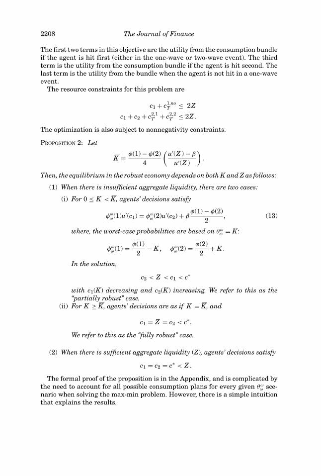
2208 The Journal of Finance
The first two terms in this objective are the utility from the consumption bundleif the agent is hit first (either in the one-wave or two-wave event). The thirdterm is the utility from the consumption bundle if the agent is hit second. Thelast term is the utility from the bundle when the agent is not hit in a one-waveevent.
The resource constraints for this problem are
c1 + c1,noT ≤ 2Z
c1 + c2 + c2,1T + c2,2
T ≤ 2Z .
The optimization is also subject to nonnegativity constraints.
PROPOSITION 2: Let
K ≡ φ(1) − φ(2)4
(u′(Z ) − β
u′(Z )
).
Then, the equilibrium in the robust economy depends on both K and Z as follows:
(1) When there is insufficient aggregate liquidity, there are two cases:
(i) For 0 ≤ K < K, agents’ decisions satisfy
φωω (1)u′(c1) = φω
ω (2)u′(c2) + βφ(1) − φ(2)
2, (13)
where, the worst-case probabilities are based on θωω = K:
φωω (1) = φ(1)
2− K , φω
ω (2) = φ(2)2
+ K .
In the solution,
c2 < Z < c1 < c∗
with c1(K) decreasing and c2(K) increasing. We refer to this as the“partially robust” case.
(ii) For K ≥ K, agents’ decisions are as if K = K, and
c1 = Z = c2 < c∗.
We refer to this as the “fully robust” case.
(2) When there is sufficient aggregate liquidity (Z), agents’ decisions satisfy
c1 = c2 = c∗ < Z .
The formal proof of the proposition is in the Appendix, and is complicated bythe need to account for all possible consumption plans for every given θω
ω sce-nario when solving the max-min problem. However, there is a simple intuitionthat explains the results.
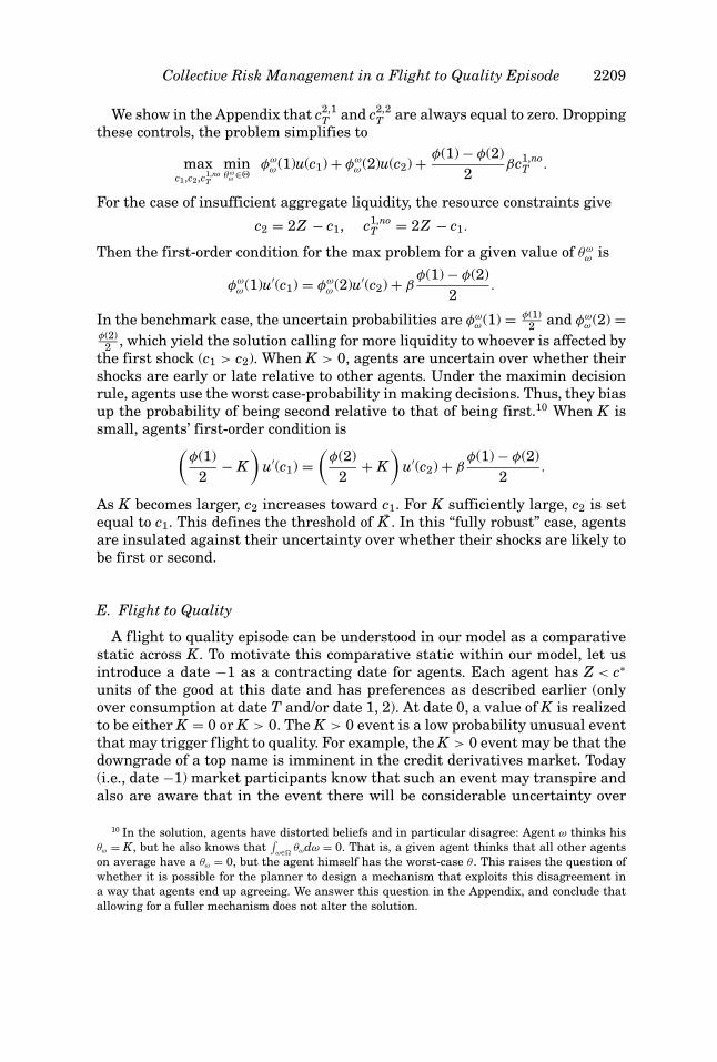
Collective Risk Management in a Flight to Quality Episode 2209
We show in the Appendix that c2,1T and c2,2
T are always equal to zero. Droppingthese controls, the problem simplifies to
maxc1,c2,c1,no
T
minθωω ∈
φωω (1)u(c1) + φω
ω (2)u(c2) + φ(1) − φ(2)2
βc1,noT .
For the case of insufficient aggregate liquidity, the resource constraints give
c2 = 2Z − c1, c1,noT = 2Z − c1.
Then the first-order condition for the max problem for a given value of θωω is
φωω (1)u′(c1) = φω
ω (2)u′(c2) + βφ(1) − φ(2)
2.
In the benchmark case, the uncertain probabilities are φωω (1) = φ(1)
2 and φωω (2) =
φ(2)2 , which yield the solution calling for more liquidity to whoever is affected by
the first shock (c1 > c2). When K > 0, agents are uncertain over whether theirshocks are early or late relative to other agents. Under the maximin decisionrule, agents use the worst case-probability in making decisions. Thus, they biasup the probability of being second relative to that of being first.10 When K issmall, agents’ first-order condition is(
φ(1)2
− K)
u′(c1) =(
φ(2)2
+ K)
u′(c2) + βφ(1) − φ(2)
2.
As K becomes larger, c2 increases toward c1. For K sufficiently large, c2 is setequal to c1. This defines the threshold of K̄ . In this “fully robust” case, agentsare insulated against their uncertainty over whether their shocks are likely tobe first or second.
E. Flight to Quality
A flight to quality episode can be understood in our model as a comparativestatic across K. To motivate this comparative static within our model, let usintroduce a date −1 as a contracting date for agents. Each agent has Z < c∗
units of the good at this date and has preferences as described earlier (onlyover consumption at date T and/or date 1, 2). At date 0, a value of K is realizedto be either K = 0 or K > 0. The K > 0 event is a low probability unusual eventthat may trigger flight to quality. For example, the K > 0 event may be that thedowngrade of a top name is imminent in the credit derivatives market. Today(i.e., date −1) market participants know that such an event may transpire andalso are aware that in the event there will be considerable uncertainty over
10 In the solution, agents have distorted beliefs and in particular disagree: Agent ω thinks hisθω = K, but he also knows that
∫ω∈�
θωdω = 0. That is, a given agent thinks that all other agentson average have a θω = 0, but the agent himself has the worst-case θ . This raises the question ofwhether it is possible for the planner to design a mechanism that exploits this disagreement ina way that agents end up agreeing. We answer this question in the Appendix, and conclude thatallowing for a fuller mechanism does not alter the solution.
2210 The Journal of Finance
outcomes. At date −1, agents enter into an arrangement, where the terms ofthe contract are contingent on the state K, as dictated by Proposition 2. We canthink of the flight to quality in comparing the contracts across the states.11
In this subsection we discuss three concrete examples of flight to qual-ity events in the context of our model. Our first two examples identify themodel in terms of the financial intermediation implementation discussed ear-lier, while the last example identifies the model in terms of the contingent claimsimplementation.
The first example is one of uncertainty-driven contagion and is drawn fromthe events of the fall of 1998. We interpret the agents of our model as thetrading desks of an investment bank. Each trading desk concentrates in a dif-ferent asset market. At date −1 the trading desks pool their capital with atop-level risk manager of the investment bank, retaining c2 of capital to coverany needs that may arise in their particular market (“committed capital”). Theyalso agree that the top-level risk manager will provide an extra c1 − c2 > 0 tocover shocks that hit whichever market needs capital first (“trading capital”).At date 0, Russia defaults. An agent in an unrelated market—that is, a marketin which shocks are now no more likely then before, so that φω
ω (1) + φωω (2) is
unchanged—suddenly becomes concerned that other trading desks will suffershocks first and hence that the agent’s trading desk will not have as muchcapital available in the event of a shock. The agent responds by lobbying thetop-level risk manager to increase his committed capital up to a level of c2 = c1.As a result, every trading desk now has less capital in the (likelier) event of asingle shock. Scholes (2000) argues that during the 1998 crisis, the natural liq-uidity suppliers (hedge funds and trading desks) became liquidity demanders.In our model, uncertainty causes the trading desks to tie up more of the capitalof the investment bank. The average market has less capital to absorb shocks,suggesting reduced liquidity in all markets.
In this example, the Russian default leads to less liquidity in other un-related asset markets. Gabaix, Krishnamurthy, and Vigneron (2006) presentevidence that the mortgage-backed securities market, a market unrelated tothe sovereign bond market, suffered lower liquidity and wider spreads in the1998 crisis. Note also that in this example there is no contagion effect if Zis large as the agents’ trading desk will not be concerned about having thenecessary capital to cover shocks when Z > c∗. Thus, any realized losses byinvestment banks during the Russian default strengthen the mechanism wehighlight.
11 An alternative way to motivate the comparative static is in terms of the rewriting of contracts.Suppose that it is costless to write contracts at date −1, but that it costs a small amount ε to writecontracts at date 0. Then it is clear that at date −1, agents will write contracts based on the K = 0case of Proposition 2. If the K > 0 event transpires, agents will rewrite the contracts accordingly.We may think of a flight to quality in terms of this rewriting of contracts. Note that the only benefitin writing a contract at date −1 that is fully contingent on K is to save the rewriting costs ε. Inparticular, if ε = 0 it is not possible to improve the allocation based on signing contingent date −1contracts. Agents are identical at both date −1 and at date 0, so that there are no extra allocationgains from writing the contracts early.
Collective Risk Management in a Flight to Quality Episode 2211
Our second example is a variant of the classical bank run, but on the creditside of a commercial bank. The agents of the model are corporates. The corpo-rates deposit Z in a commercial bank at date −1 and sign revolving credit linesthat give them the right to c1 if they receive a shock. The corporates are alsoaware that if banking conditions deteriorate (a second wave of shocks) the bankwill raise lending standards/loan rates so that the corporates will effectivelyreceive only c2 < c1. The flight to quality event is triggered by the commercialbank suffering losses and corporates becoming concerned that the two-waveevent will transpire. They respond by preemptively drawing down credit lines,effectively leading all firms to receive less than c1. Gatev and Strahan (2006)present evidence of this sort of credit line run during periods when the spreadbetween commercial paper and Treasury bills widens (as in the fall of 1998).
The last example is one of the interbank market for liquidity and the paymentsystem. The agents of the model are all commercial banks that have Z Treasurybills at the start of the day. Each commercial bank knows that there is somepossibility that it will suffer a large outflow from its reserve account, which itcan offset by selling Treasury bills. To fix ideas, suppose that bank A is worriedabout this happening at 4pm. At date −1, the banks enter into an interbanklending arrangement so that a bank that suffers such a shock first, receivescredit on advantageous terms (worth c1 of T-bills). If a second set of shockshits, banks receive credit at worse terms of c2 (say, the discount window). Atdate 0, 9/11 occurs. Suppose that bank A is a bank outside New York City thatis not directly affected by the events, but that is concerned about a possiblereserve outflow at 4pm. However, now bank A becomes concerned that othercommercial banks will need liquidity and that these needs may arise before4pm. Then bank A will renegotiate its interbank lending arrangements andbecome unwilling to provide c1 to any banks that receive shocks first. Rather,it will hoard its Treasury bills of Z to cover its own possible shock at 4pm. Inthis example, uncertainty causes banks to hoard resources, which is often thesystemic concern in a payments gridlock (e.g., Stewart (2002) and McAndrewsand Potter (2002)).
The different interpretations we have offered show that the model’s agentsand their actions can be mapped into the actors and actions during a flight toquality episode in a modern financial system. As is apparent, our environmentis a variant of the one that Diamond and Dybvig (1983) study. In that model, thesequential service constraint creates a coordination failure and the possibilityof a bad crisis equilibrium in which depositors run on the bank. In our model,the crisis is a rise in Knightian uncertainty rather than the realization of thebad equilibrium. The association of crises with a rise in uncertainty is thenovel prediction of our model, and one that fits many of the flight to qualityepisodes we have discussed in this paper. Other variants of the Diamond andDybvig model such as Rochet and Vives (2004) associate crises with low values ofcommercial bank assets. While our model shares this feature (i.e., Z must be lessthan c∗), it provides a sharper prediction through the uncertainty channel. Ourmodel also offers interpretations of a crisis in terms of the rewriting of financialcontracts triggered by an increase in uncertainty, rather than the behavior of
2212 The Journal of Finance
a bank’s depositors. Of course, in practice both the coordination failures thatDiamond and Dyvbig highlight and the uncertainties we highlight are likely tobe present, and may interact, during financial crises.
II. Collective Bias and the Value of Intervention
In this section, we study the benefits of central bank actions in the flightto quality episode of our model. We show that a central bank can interveneto improve aggregate outcomes. The analysis also clarifies the source of thebenefit in our model.
A. Central Bank Information and Objective
The central bank knows the aggregate probabilities φ(1) and φ(2), and knowsthat the φω ’s are drawn from a common distribution for all ω. We previouslynote that this information is common knowledge, so we are not endowing thecentral bank with any more information than agents have. The central bankalso understands that because of agents’ ex ante symmetry, all agents choose thesame contingent consumption plan Cs. We denote by ps,CB
ω the probabilities thatthe central bank assigns to the different events that may affect agent ω. Likeagents, the central bank does not know the true probabilities ps
ω. Additionally,ps,CB
ω may differ from ps,ωω .
The central bank is concerned with the equally weighted ex post utility thatagents derive from their consumption plans:
V CB ≡∫
ω∈�
∑ps,CB
ω U (Cs) dω
=∑
psU (Cs).(14)
The step in going from the first to second line is an important one in the analysis.In the first line, the central bank’s objective reflects the probabilities for eachagent ω. However, since the central bank is concerned with the aggregate out-come, we integrate over agents, exchanging the integral and summation, andarrive at a central bank objective that only reflects the aggregate probabilitiesps. Note that the individual probability uncertainties disappear when aggregat-ing, and that the aggregate probabilities that appear are common knowledge(i.e., they can be written solely in terms of φ(1) and φ(2)). Finally, as our ear-lier analysis has shown that only c1, c2, c1,no
T > 0 need to be considered, we canreduce the objective to
V CB = φ(1)2
u(c1) + φ(2)2
u(c2) + φ(1) − φ(2)2
βc1,noT .
The next two subsections explain how a central bank that maximizes theobjective function in (14) will intervene. For now, we note that one can view theobjective in (14) as descriptive of how central banks behave: Central banks are
Collective Risk Management in a Flight to Quality Episode 2213
interested in the collective outcome, and thus it is natural that the objectiveadopts the average consumption utility of agents in the economy. We return toa fuller discussion of the objective function in Section D where we explain thiscriterion in terms of welfare and Pareto improving policies.
B. Collective Risk Management and Wasted Liquidity
Starting from the robust equilibrium of Proposition 2, consider a central bankthat alters agents’ decisions by increasing c1 by an infinitesimal amount, anddecreasing c2 and c1,no
T by the same amount. The value of the reallocation basedon the central bank objective in (14) is
φ(1)2
u′(c1) − φ(2)2
u′(c2) − φ(1) − φ(2)2
β. (15)
First, note that if there is sufficient aggregate liquidity, c1 = c2 = c∗ = u′−1(β).For this case,
φ(1)2
u′(c1) − φ(2)2
u′(c2) − φ(1) − φ(2)2
β = 0
and equation (15) implies that there is no gain to the central bank from areallocation.
Turning next to the insufficient liquidity case, the first-order condition foragents in the robustness equilibrium satisfies
φωω (1)u′(c1) − φω
ω (2)u′(c2) − βφ(1) − φ(2)
2= 0,
or (φ(1)
2− K
)u′(c1) −
(φ(2)
2+ K
)u′(c2) − β
φ(1) − φ(2)2
= 0.
Rearranging this equation we have that
φ(1)2
u′(c1) − φ(2)2
u′(c2) − βφ(1) − φ(2)
2= K (u′(c1) + u′(c2)).
Substituting this relation into (15), it follows that the value of the reallocationto the central bank is K(u′(c1) + u′(c2)), which is positive for all K > 0. That is,the reallocation is valuable to the central bank because, from its perspective,agents are wasting aggregate liquidity by self-insuring excessively rather thancross-insuring risks.
Summarizing these results:
PROPOSITION 3: For any K > 0, if the economy has insufficient aggregate liq-uidity (Z < c∗), on average agents choose too much insurance against receivingshocks second relative to receiving shocks first. A central bank that maximizes
2214 The Journal of Finance
the expected (ex post) utility of agents in the economy can improve outcomes byreallocating agents’ insurance toward the first shock.
C. Is the Central Bank Less Knightian or More Informed than Agents?
In particular, are these the reasons the central bank can improve outcomes?The answer is no. To see this, note that any randomly chosen agent in thiseconomy would reach the same conclusion as the central bank if charged withoptimizing the expected ex post utility of the collective set of agents.
Suppose that agent ω̃, who is Knightian and uncertain about the true valuesof θω, is given such a mandate. Then this agent will solve
maxc1,c2,c1,no
T
minθω̃ω ∈
∫ (φω̃
ω (1)u(c1) + φω̃ω (2)u(c2) + φ(1) − φ(2)
2βc1,no
T
)dω.
Since aggregate probabilities are common knowledge we have that∫φω̃
ω (1) dω = φ(1)2
,∫
φω̃ω (2) dω = φ(2)
2.
Substituting these expressions back into the objective and dropping the minoperator (since now no expression in the optimization depends on θω̃
ω ) yields
maxc1,c2,c1,no
T
φ(1)2
u(c1) + φ(2)2
u(c2) + φ(1) − φ(2)2
βc1,noT ,
which is the same objective as that of the central bank.If it is not an informational advantage or the absence of Knightian traits in
the central bank, what is behind the gain we document? The combination oftwo features drives our results: The central bank is concerned with aggregatesand individual agents are “uncertain” (Knightian) not about aggregate shocksbut about the impact of these shocks on their individual outcomes.
Since individual agents make decisions about their own allocation of liquidityrather than about the aggregate, they make choices that are collectively biasedwhen looked at from the aggregate perspective. Let us develop the collectivebias concept in more detail.
In the fully robust equilibrium of Proposition 2 agents insure equally againstfirst and second shocks. To arrive at the equal insurance solution, robust agentsevaluate their first order conditions (equation 13) at conservative probabilities:
φωω (1) − φω
ω (2) = φ(1) − φ(2)2
(u′(c∗)u′(Z )
). (16)
Suppose we compute the probability of one and two aggregate shocks usingagents’ conservative probabilities:
φ̄(1) ≡ 2∫
�
φωω (1) dω, φ̄(2) ≡ 2
∫�
φωω (2) dω.
Collective Risk Management in a Flight to Quality Episode 2215
The “2” in front of these expressions reflects the fact that only one-half of theagents are affected by each of the shocks. Integrating equation (16) and usingthe definitions above, we find that agents’ conservative probabilities are suchthat
φ̄(1) − φ̄(2) = (φ(1) − φ(2))(
u′(c∗)u′(Z )
)< φ(1) − φ(2).
The last inequality follows in the case of insufficient aggregate liquidity (Z <
c∗).Implicitly, these conservative probabilities overweight an agent’s chances of
being affected second in the two-wave event. Since each agent is concernedabout the scenario in which he receives a shock last and there is little liquidityleft, robustness considerations lead each agent to bias upwards the probabilityof receiving a shock later than the average agent. However, every agent cannotbe later than the “average.” Across all agents, the conservative probabilitiesviolate the known probabilities of the first- and second-wave events.
Note that each agent’s conservative probabilities are individually plausible.Given the range of uncertainty over θω, it is possible that agent ω has a higherthan average probability of being second. Only when viewed from the aggregatedoes it become apparent that the scenario that the collective of conservativeagents are guarding against is impossible.
D. Welfare
We next discuss our specification of the central bank’s objective in (14). Agentsin our model choose the worst case among a class of priors when making deci-sions. That is, they are not rational from the perspective of Bayesian decisiontheory and therefore do not satisfy the Savage axioms for decision making. AsSims (2001) notes, this departure from rational expectations can lead to a situ-ation where a maximin agent accepts a series of bets that have him lose moneywith probability one. The appropriate notion of welfare in models where agentsare not rational is subject to some debate in the literature.12 It is beyond thescope of this paper to settle this debate. Our aim in this section is to clarify theissue in the present context and offer some arguments in favor of objective (14).
At one extreme, consider a “libertarian” welfare criterion whereby agents’choices are by definition what maximizes their utility. That is, define
V CB =∫
ω∈�
minθωω ∈
∑ps,ω
ω U (Cs) dω.
This is an objective function based on each agent ω’s ex ante utility, which isevaluated using that agent’s worst-case probabilities. The difference relative tothe objective in (14) is that all utility here is “anticipatory.” That is, the agent
12 The debate centers on whether or not the planner should use the same model to describe choicesand welfare (see, for example, Gul and Pesendorfer (2005) and Bernheim and Rangel (2005) fortwo sides of the argument). See also Sims (2001) in the context of a central bank’s objective.
2216 The Journal of Finance
enjoys happiness at date 0 from making a decision that avoids a worst-caseoutcome. Note that such a specification differs from standard expected utilitywhereby the agent only receives happiness at dates 1, 2, and T when the agentactually consumes.
Under the objective V CB the agent’s choices are efficient and there is no rolefor the central bank. We can see this immediately because the planning problemin deriving Proposition 2 was based on the latter objective function.
The objective function we use in (14) is based on ex post consumption utility,and assumes that agents do not receive any anticipatory utility. More generally,consider an objective function λ V CB + (1 − λ)V CB with λ ∈ [0, 1]. Then it isclear that as long as λ < 1, that is, the welfare function places some weight onex post consumption utility, there is a role for the central bank. In this sense,the no-intervention case is an extreme one.
There is a further reason to restrict attention to the λ = 0 case, as in (14).Consider the following thought experiment: Suppose that we repeat infinitelymany times the liquidity episode we have described. At the beginning of eachepisode, agent ω draws a θω ∈ . These draws are i.i.d. across episodes, and theagent knows that on average his θω will be zero. In each episode, since agentω does not know the θω for that episode, the agent’s worst-case decision rulehas him using θω = K. Then, VCB is the average consumption utility of agent ω
across all of these episodes.13
The preceding two arguments are ones in favor of using an ex post consump-tion utility welfare criterion, where each agent is weighted equally. The lastpoint we discuss is when equal weighting is appropriate. Thus far, since agentsare ex ante identical, a policy that improves the average agent’s ex post con-sumption utility also improves each agent’s ex post expected consumption util-ity. Suppose, however, that a fraction of the agents in the economy are Bayesian(i.e., rational) and they know that their true θω is equal to K. For these agents,the worst-case probabilities are truly their own probabilities. Thus, define thewelfare of the rational agents as
V R =∫
ω∈�R
∑ps,ω
ω U (Cs) dω,
where �R is the subset of � corresponding to the rational agents, and the prob-abilities ps,ω
ω are based on θω = K.The rest of the agents, ω ∈ � \ �R, are Knightian with θωs such that the
average θω across both classes of agents is zero. We define VK in a similarway to the objective in (14) as the average ex post consumption utility of theKnightian agents.
We now have a situation where there is ex ante heterogeneity among agentsso that equal weighting is no longer appropriate. Suppose that the central bank
13 Of course, in living through repeated liquidity events, an agent learns over time about thetrue distribution of θω. However, it is still the case that along this learning path, K remains strictlypositive (while shrinking) and hence the qualitative features of our argument go through for asmall enough discount rate.
Collective Risk Management in a Flight to Quality Episode 2217
cannot discriminate among the two classes of agents. Is the intervention stillPareto improving?
The result in Proposition 3 still applies to the Knightian agents. The centralbank will compute a first-order gain in VK from the reallocation intervention.Importantly, note that the envelope theorem implies that changing the rationalagents’ decisions results in only a second-order utility loss to the rational agents.That is, a small intervention means that the loss in VR is small compared to thegain in VK . Thus, although the central bank’s policy is not Pareto improving,it involves asymmetric gains to the Knightian agents. Camerer et al. (2003)propose this type of asymmetric paternalism criterion in evaluating policieswhen some agents are behavioral.
E. Risk Aversion versus Uncertainty Aversion
We note previously that from a positive standpoint our model of uncertaintyaversion predicts a flight to quality when there is a “new” shock, whereas amodel with extreme risk aversion predicts conservative behavior in responseto any negative shock, new or not. We close this section by noting that thenormative implications of uncertainty aversion also differ from that of extremerisk aversion. Without collective bias, and regardless of the agent’s degree ofrisk aversion, our central bank sees no reason to reallocate liquidity toward thefirst wave of shocks beyond the private sector’s choices. We can see this becausesetting K = 0 in our model represents a model without uncertainty aversion.As we have imposed only weak requirements on u(·), the utility function canbe chosen to represent extreme forms of risk aversion. However, the results ofProposition 3 establish that there is a gain for the central bank only if K > 0and Z < c∗.
We conclude that there is a role for the central bank only in situations ofKnightian uncertainty and insufficient aggregate liquidity. Of course not allrecessionary episodes exhibit these ingredients. But there are many scenariosin which they are present, such as during October 1987 and in the fall of 1998.
III. An Application: Lender of Last Resort
The abstract reallocation experiment considered in Proposition 3 makes clearthat during flight to quality episodes the central bank will find it desirableto induce agents to insure less against second shocks and more against firstshocks. In this section we discuss an application of this result and consider alender of last resort (LLR) policy in light of the gain identified in Proposition 3.
As in Woodford (1990) and Holmstrom and Tirole (1998), we assume the LLRhas access to collateral that private agents do not (or at least, it has access ata lower cost). Woodford and Holmstrom and Tirole focus on the direct valueof intervening using this collateral. Our novel result is that, because of thereallocation benefit of Proposition 3, the value of the LLR exceeds the directvalue of the intervention. Thus, our model sheds light on a new benefit of theLLR.
2218 The Journal of Finance
The model also stipulates when the benefit is highest. As we have remarkedpreviously, the reallocation benefit only arises in situations where K > 0 andZ < c∗. This carries over directly to our analysis of the LLR: The benefits arehighest when K > 0 and Z < c∗. We also show that the LLR must be a last resortpolicy. If liquidity injections take place too often, the reallocation effect worksagainst the policy and reduces its value.
A. LLR Policy
Formally, the central bank credibly expands the resources of agents in thetwo-shock event by an amount ZG. That is, agents who are affected second inthe two-wave event (s = (2, 2)), will have their consumption increased from c2to c2 + 2ZG (twice ZG because one-half measure of agents are affected by thesecond shock). The resource constraints for agents (for the reduced problem)are
c1 + c1,noT ≤ 2Z (17)
c1 + c2 ≤ 2Z + 2Z G . (18)
In practice, the central bank’s promise may be supported by a credible commit-ment to costly ex post inflation or taxation and carried out by guaranteeing,against default, the liabilities of financial intermediaries who have sold finan-cial claims against extreme events. Since we are interested in computing themarginal benefit of intervention, we study an infinitesimal intervention of ZG.
If the central bank offers more insurance against the two-shock event, thisinsurance has a direct benefit in terms of reducing the disutility of an adverseoutcome. The direct benefit of the LLR is
V CB,directZ G = 2
∫�
φω(2)u′(c2,ω) dω = φ(2)u′(c2).
The anticipation of the central bank’s second-shock insurance leads agentsto re-optimize their insurance decisions. Agents reduce their private insuranceagainst the publicly insured second-shock and increase their first-shock insur-ance. The total benefit of the intervention includes both the direct benefit aswell as any benefit from portfolio re-optimization:
V CB,totalZ G =
∫�
[φω(1)u′(c1,ω)
dc1,ω
dZG + φω(2)u′(c2,ω)dc2,ω
dZG + φ(1) − φ(2)2
βdc1,no
T ,ω
dZG
]dω.
From (13), the first-order condition for agent decisions in the robust equilibriumgives
φ(1)2
u′(c1) = φ(2)2
u′(c2) + βφ(1) − φ(2)
2+ K (u′(c1) + u′(c2)).
We simplify the expression for V CB,totalZ G by integrating through φω(1) and φω(2)
and then substituting for u′(c1) from the first-order condition. These operations
Collective Risk Management in a Flight to Quality Episode 2219
yield
V CB,totalZ G = φ(2)
2u′(c2)
(dc1
dZG + dc2
dZG
)+ β
φ(1) − φ(2)2
(dc1
dZG + dc1,noT
dZG
)
+ K (u′(c1) + u′(c2))dc1
dZG .
Last, we differentiate the resource constraints (17) and (18) with respect to ZG
to find
dc1
dZG + dc2
dZG = 2,dc1
dZG + dc1,noT
dZG = 0.
We have
V CB,totalZ G = φ(2)u′(c2) + K (u′(c1) + u′(c2))
dc1
dZG
= V CB,directZ G + K (u′(c1) + u′(c2))
dc1
dZG .
The additional benefit we identify is due to portfolio re-optimization: Agents cutback on the publicly insured second shock and increase first-shock insurance,thereby moving their decisions closer to what the central bank would choose forthem. In this sense, the LLR policy can help to implement the policy suggestedin Proposition 3.
We also note that without Knightian uncertainty (K = 0), there is no gain(beyond the direct benefit) from the policy. Moreover, it is straightforward tosee that if Z > c∗, then agents will not use the additional insurance to covertheir liquidity shocks, but will re-optimize in a way as to use the insuranceat date T. In this case there is no gain to offering the public insurance (sincedc1
dZG = 0). We summarize these results as follows:
PROPOSITION 4: For K > 0 and Z < c∗, the total value of the lender of last resortpolicy exceeds its direct value:
V CB,totalZ G > V CB,direct
Z G .
It is important to note that under the LLR policy the central bank injectsresources only rarely. As we associate the second-shock event with an extremeand unlikely event, in expectation the central bank does not promise manyresources. This aspect of policy is similar to Diamond and Dybvig’s (1983) anal-ysis of a LLR. However, there are a few important differences in the mecha-nism through which the policies work. As there is no coordination failure in ourmodel, the policy does not work by ruling out a “bad” equilibrium. Rather, thepolicy works by reducing the agents’ “anxiety” that they will receive a shock lastwhen the economy has depleted its liquidity resources. It is this anxiety thatleads agents to use a high φω
ω (2) in their decision rules. From this standpoint,
2220 The Journal of Finance
it is also clear that an important ingredient in the policy is that agents have tobelieve that the central bank will have the necessary resources in the two-eventshock to reduce their anxiety. Credibility and commitment are central to theworking of our LLR policy.14
B. Moral Hazard and Early Interventions
The policy we have suggested cuts against the usual moral hazard critique ofcentral bank interventions. The moral hazard critique is predicated on agentsresponding to the provision of public insurance by cutting back on their owninsurance activities. In our model, in keeping with the moral hazard critique,agents reallocate insurance away from the publicly insured shock. However,when flight to quality is the concern, the reallocation improves (ex post) out-comes on average.15 Public and private provision of insurance are complementsin our model.
This logic suggests that interventions against first shocks may be subjectto the moral hazard critique as agents’ portfolio re-optimization would leadthem toward more insurance against the second shock. To consider the “earlyintervention” case, suppose that the central bank credibly offers to increase theconsumption of agents who are affected in the first shock from c1 to c1 + 2ZG.The resource constraints for agents (for the reduced problem) are
c1 + c1,noT ≤ 2Z + 2Z G
c1 + c2 ≤ 2Z + 2Z G .
The direct benefit of intervention in the first shock is
V CB,direct,firstZ G = 2
∫�
φω(1) u′(c1,ω) dω = φ(1) u′(c2).
We compute the total benefit as previously except that we substitute agents’first-order condition using
φ(2)2
u′(c2) = φ(1)2
u′(c1) − βφ(1) − φ(2)
2− K (u′(c1) + u′(c2)).
Also, using the fact that
dc1
dZG + dc2
dZG = 2,dc1
dZG + dc1,noT
dZG = 2,
14 In this sense the policy relates to the government bond policy of Woodford (1990) andHolmstrom and Tirole (1998) who argue that government promises are unique because they havegreater collateral backing than private sector promises.
15 Note that if the direct effect of intervention is insufficient to justify intervention, then thelender of last resort policy is time inconsistent. This result is not surprising as the benefit of thepolicy comes precisely from the private sector reaction, not from the policy itself.
Collective Risk Management in a Flight to Quality Episode 2221
we find that
V CB,totalZ G = V CB,direct,first
Z G − K (u′(c1) + u′(c2))dc1
dZG < V CB,direct,firstZ G .
The expected cost of the early intervention policy is much larger than thesecond-shock intervention, since the central bank rather than the private sec-tor bears the cost of insurance against the (likely) single-shock event. Agentsreallocate the expected resources from the central bank to the two-shock event,which is exactly the opposite of what the central bank wants to achieve. In thissense, interventions in intermediate events are subject to the moral hazardcritique. We conclude that the lender of last resort facility, to be effective andimprove private financial markets, has to be a last and not an intermediateresort.
C. Multiple Shocks
It is clear that the LLR should not intervene during early shocks and insteadshould only pledge resources for late shocks; but if we move away from ourtwo-shock model to a more realistic context with multiple potential waves ofaggregate shocks, how late is late?
To answer this question we extend the model to consider multiple shocks. Weassume the economy may experience n = 1 . . . N waves of shocks, each affecting1N of the agents. The probability of the economy experiencing n waves is denotedφ(n), with φ(n) < φ(n − 1). Also, each ω ’s probability of being affected in the nthwave satisfies
∫ω∈�
φω(n) dω = φ(n)N .
The LLR policy takes the following form: The central bank injects 1N− j+1
units of liquidity for all shocks after (and including) the jth wave (j ≤ N). Wealso simplify our analysis by focusing on the fully robust case in which cn is thesame for all n and by setting β = 0, thereby assuring that Z < c∗ and allowing usto disregard effects on cn,no
T . The term cn rises to cn + NN− j+1 in the intervention
(i.e., 1N− j+1 injected to a measure 1
N of agents).The direct value of the intervention as a function of j is
V CB,directZ G = N
N − j + 1
∫�
N∑n= j
φω(n)u′(cn,ω) dω
= u′(c1) 1N− j+1
N∑n= j
φ(n).
Agents reduce insurance against the publicly insured shocks and increasetheir private insurance for the rest of the shocks. The total benefit of the in-tervention includes both the direct benefit as well as any benefit from portfolio
2222 The Journal of Finance
re-optimization:
V CB,totalZ G =
∫�
N∑n=1
φω(n)u′(cn,ω)dcn,ω
dZG dω.
From the resource constraint we have thatN∑
n=1
dcn,ω
dZG = N .
In the fully robust case, cn,ω and dcn,ω
dZG are the same for all n. We then have
V CB,totalZ G = u′(c1)
dc1
dZG
1N
N∑n=1
φ(n) = u′(c1)1N
N∑n=1
φ(n). (19)
Note that this expression is independent of the intervention rule j. In contrast,it is apparent that V CB,direct
Z G is decreasing with respect to j since the φ(n)’s aremonotonically decreasing. Thus, the ratio
V CB,totalZ G
V CB,directZ G
=1N
∑Nn=1 φ(n)
1N− j+1
∑Nn= j φ(n)
is strictly greater than one for all j > 1 and is increasing with respect to j.Of course, the above result does not suggest that intervention should occur
only in the Nth shock. Instead, it suggests that for any given amount of re-sources available for intervention, the LLR should first pledge resources to theNth shock and continue to do so until it completely replaces private insurance;it should then move on to the N − 1st shock, and so on.
The multiple shock model also clarifies another benefit of late intervention.As j rises, events that are being insured by the LLR become increasingly lesslikely. If we take the case where the shadow cost of the LLR resources for thecentral bank is constant, the expected cost of the LLR policy falls as j rises,while the expected benefit remains constant.
In other words, as j rises, it is the private sector that increasingly improves theallocation of scarce private resources to early and more likely aggregate shocks,thereby reducing the extent of the flight to quality phenomenon. In contrast,the central bank plays a decreasingly small role in terms of the expected valueof resources actually disbursed as j increases.
Thus, while a well-designed LLR policy may indeed have a direct effect onlyin highly unlikely events, the policy is not irrelevant for likely outcomes. Itsmain benefits come from unlocking private markets to insure more likely andless extreme events.
IV. Final Remarks
We present a model of financial crises and the role of a lender of last re-sort that centers on Knightian uncertainty and liquidity shortages. While
Collective Risk Management in a Flight to Quality Episode 2223
Knightian uncertainty is discussed in policy circles (e.g., see Greenspan’s quotein the Introduction), it is not standard in academic analyses of crises, whichinstead emphasize liquidation externalities (e.g., Diamond and Dybvig (1983)).Thus, rather than ending with a summary of findings, it is useful to take stock byconsidering points of similarity and departure between our Knightian uncer-tainty model and the standard liquidation externality model.
As we argue throughout the paper, an “uncertainty shock,” distinct from—although possibly correlated with—a liquidation shock is an important elementin many financial crises. The uncertainty shock, like the liquidation shock,reproduces the behavior of agents during a flight to quality episode. Agentsmove toward holding uncontingent and safe assets, financial intermediarieshoard liquidity, and investment banks and trading desks turn conservative intheir allocation of risk capital so that capital becomes immobile across markets.On these points our model emphasizes a different mechanism but shares manyof the predictions of liquidation models.
Despite this similarity, we think it is valuable to spell out the model of theuncertainty shock. At a minimum, doing so clarifies and expands the set of pre-conditions for crises. There may be crisis events where liquidation externalitiesare absent but in which there is a substantial amount of Knightian uncertainty.At the other extreme, the most severe crises in the U.S. and abroad seem tohave elements of both an uncertainty and a liquidation shock. In such casesour model helps to understand why these crises may have been so severe.
Furthermore, there are some events—for example, the recent liquidation ofthe Amaranth hedge fund’s sizeable portfolio—for which the preconditions seemto fit the liquidation crisis model, but yet did not trigger crises. Our modelsuggests that the absence of significant uncertainty around these events maybe one reason why (in the particular case of Amaranth, financial specialistshad already learned from the LTCM experience). Thus, our model also helpsto shed light on the “dog that did not bark.” More broadly, it suggests thatan important precondition for crises is the presence of “new” shocks, perhapssurrounding new and untested financial innovations. This prediction is alsouseful to guide policymakers on where crises may arise.
From a policymaker’s perspective, our model, like the liquidation externalitymodel, shows that there are benefits to a lender of last resort facility duringa crisis. However, in our model the central issue to determine the value ofan LLR facility is not only the potential for coordination failure but also theextent of uncertainty in the marketplace. For example, we prescribe that adefault by a hedge fund—even one that is large—should not elicit a centralbank reaction unless the default triggers considerable uncertainty in othermarket participants and hedge funds are financially weak.
Yet another subtle difference between the two models is in the incentiveeffects of policy intervention. In the liquidation model, moral hazard is oftenan important issue that tempers policy intervention. This is because privateand public insurance are substitutes in this model. In contrast, our analysisreveals that in the uncertainty model there are dimensions in which privateand public insurance are complements rather than substitutes, suggesting that
2224 The Journal of Finance
the moral hazard issue is less important for uncertainty driven crises. Havingsaid this, a different kind of moral hazard problem may arise in the uncertaintymodel if agents can invest resources to affect the degree of uncertainty theyface.
In the liquidation model, ex ante policy recommendations typically center onprudential risk management. For example, in many analyses there are exter-nalities present that drive a wedge between private and social incentives toinsure against a financial crisis episode. In such scenarios, ex ante regulationsto reduce leverage, increase liquidity ratios, or tighten capital requirementsare beneficial. In our model, an important dimension of the crisis is that thereis uncertainty about outcomes. Agents cannot refer to history to understandhow a crisis will unfold because the historical record may not span the eventspace. In such a case it is unclear whether any entity, private or public, canarrive at the appropriate ex ante risk management strategy, calling into ques-tion the feasibility of these policy recommendations. Instead, in our uncertaintymodel, the most beneficial ex ante actions are ones that help to reduce the ex-tent of uncertainty should a crisis occur. In some cases, this may simply involvemaking common knowledge information that is known to subsets of marketparticipants—for example, making common knowledge the portfolio positionsof the major players in a market. In other cases, this may involve the centralbank facilitating discussions among the private sector on how each party willreact in a crisis scenario.
These points are pertinent, and can be illustrated, in the credit derivativesmarket. There is currently considerable uncertainty over how the downgradeof a top name will affect the credit derivatives market (see Geithner (2006)).16
Market participants are aware that such a downgrade will occur at some point,but given the lack of history, they are uncertain of how events will unfold. Willthe market absorb such a shock without losing liquidity? Could such a shockresult in a credit crunch that causes the corporate sector to suffer, and trigger adomino effect of downgrades? Are back-office and settlement procedures suffi-cient to handle such an event? Our model suggests that the central bank standsready to act as the LLR in the event that a downgrade triggers these uncer-tainties. There have also been recent moves to increase transparency and riskassessment in this market, as well as streamline back-office settlement proce-dures. Our model suggests that such ex ante actions may reduce uncertaintyand be beneficial.
Finally, as we note, Knightian uncertainty may often be associated withfinancial innovations. This suggests that crises surrounding financial innova-tions may by fertile ground to look empirically for the effects we have modeled,and disentangle them from other more well understood effects. It also suggestsa new perspective on the costs and benefits of innovation. For example, ourmodel suggests that in a dynamic context with endogenous financial innova-tion, it is the pace of this innovation that inherently creates uncertainty and
16 The model may also be applied to the subprime crisis, as we discuss in Caballero andKrishnamurthy (2008).
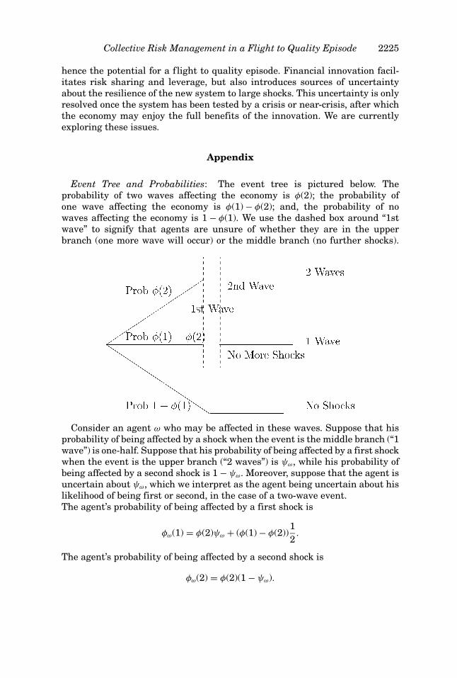
Collective Risk Management in a Flight to Quality Episode 2225
hence the potential for a flight to quality episode. Financial innovation facil-itates risk sharing and leverage, but also introduces sources of uncertaintyabout the resilience of the new system to large shocks. This uncertainty is onlyresolved once the system has been tested by a crisis or near-crisis, after whichthe economy may enjoy the full benefits of the innovation. We are currentlyexploring these issues.
Appendix
Event Tree and Probabilities: The event tree is pictured below. Theprobability of two waves affecting the economy is φ(2); the probability ofone wave affecting the economy is φ(1) − φ(2); and, the probability of nowaves affecting the economy is 1 − φ(1). We use the dashed box around “1stwave” to signify that agents are unsure of whether they are in the upperbranch (one more wave will occur) or the middle branch (no further shocks).
Consider an agent ω who may be affected in these waves. Suppose that hisprobability of being affected by a shock when the event is the middle branch (“1wave”) is one-half. Suppose that his probability of being affected by a first shockwhen the event is the upper branch (“2 waves”) is ψω, while his probability ofbeing affected by a second shock is 1 − ψω. Moreover, suppose that the agent isuncertain about ψω, which we interpret as the agent being uncertain about hislikelihood of being first or second, in the case of a two-wave event.The agent’s probability of being affected by a first shock is
φω(1) = φ(2)ψω + (φ(1) − φ(2))12
.
The agent’s probability of being affected by a second shock is
φω(2) = φ(2)(1 − ψω).
2226 The Journal of Finance
Note that
φω(1) + φω(2) = φ(2) + (φ(1) − φ(2))12
= φ(1) + φ(2)2
,
and
φω(1) − φ(1)2
= φ(2)ψω − φ(2)2
φω(2) − φ(2)2
= −φ(2)ψω + φ(2)2
.
These expressions show that the event tree is consistent with agents beingcertain about their probability of receiving a shock, but being uncertain abouttheir relative probabilities of being first or second. In the text, we describe theuncertainty in terms of φω(2) − φ(2)
2 rather than in terms of ψω.Proof of Proposition 2: We focus on the case of insufficient aggregate liquidity
(Z < c∗). The other case follows the same logic as the K = 0 case. We are lookingfor a solution to the problem in equation (12). We can describe this problemin the game-theoretic language often used in max-min problems. The agentchooses C to maximize V (C; θω
ω ) anticipating that “nature” will choose θωω to
minimize V (C; θωω ) given the agent’s choice of C.
The solution (θ̄ωω, C̄) has to satisfy a pair of optimization problems. First, θ̄ω
ω ∈argminθω
ωV (C̄; θω
ω ). That is, nature chooses θωω optimally given the agent’s choice
of C̄. Second, C̄ ∈ argmaxCV (C; θ̄ωω). That is, the agent chooses C optimally given
nature’s choice of θ̄ωω.17
We compute
∂V∂θω
ω
= u(c2) − u(c1) + β(c2,2
T − c2,1T
).
Let us first ask whether there exists a solution in which ∂V∂θω
ω< 0. If so, then
clearly θωω = +K. Taking this value of θω
ω let us consider the agent’s problem inequation (12). First note that c2,1
T = 0. To see this, suppose that c2,1T > 0. Then
we can reduce c2,1T by δ and increase c2,2
T by δ and produce a utility gain ofδ(φω
ω (2) − φ(2) + φωω (2)) > 0 when θω
ω > 0.With this knowledge, we rewrite the condition that ∂V
∂θωω
< 0 as,
u(c2) + βc2,2T < u(c1) ⇒ c1 > c2.
If c1 > c2 and Z < c∗ it follows from the resource constraint that c2 < c∗. But ifc2 < c∗ then from the agent’s problem we must have that c2,2
T = 0 (i.e., do notsave any resources for date T if these resources could be used earlier).
17 The fact that the agent chooses C before nature chooses θωω does not affect our problem. To
see this, note that choosing first only gives the agent an advantage if the agent can induce natureto choose a θω
ω different from θ̄ ωω. Suppose the agent chooses C �= C̄ to increase V(·). Clearly, this
choice reduces V below V (θ̄ ωω, C̄). Thus, nature can always choose to set θω
ω = θ̄ ωω and make the agent
strictly worse off than at the choice C = C̄.
Collective Risk Management in a Flight to Quality Episode 2227
Thus, we only need to consider the agent’s problem in (12) for values ofc1, c2, c1,no
T > 0. The first-order condition for the agent at θωω = +K is(
φ(1)2
− K)
u′(c1) =(
φ(2)2
+ K)
u′(c2) + βφ(1) − φ(2)
2.
We note that for K = 0, the unique solution to the agent’s problem is c1 > c2.Thus, for small values of K, a solution exists in which the agent chooses c1 > c2and nature chooses θω
ω = +K. This is the partially robust solution given in theproposition.
As K becomes larger, c1/c2 falls and at some point c1 = c2 = Z . This occurswhen K solves(
φ(1)2
− K)
u′(Z ) =(
φ(2)2
+ K)
u′(Z ) + βφ(1) − φ(2)
2,
which gives the expression for the value of K defined in the proposition.Note that if K > K, the solution θω
ω = +K and c1 = c2 still solves both theagent’s and nature’s optimization problems. The agent’s choice is uniquely op-timal at θω
ω = +K, while nature is indifferent over values of θωω ∈ [−K, +K]. This
is the fully robust solution given in the proposition.We have thus far shown that considering the case in which ∂V
∂θωω
≤ 0, thesolution given in the proposition is the only solution to the problem in (12).We conclude by showing that there are no other solutions to the problem. Todo this, we only need to consider whether there exists a solution in which∂V∂θω
ω> 0.
Suppose there does exist such a solution. If ∂V∂θω
ω> 0, then θω
ω = −K. We cango back through arguments similar to those previously offered to show thatc2,2
T and c2,1T must both be zero in this case. Then the condition that ∂V
∂θωω
> 0 isequivalent to
c1 < c2.
The first-order condition for the agent is
(φ(1)
2+ K
)u′(c1) =
(φ(2)
2− K
)u′(c2) + β
φ(1) − φ(2)2
.
The solution to this problem is c1 > c2, which is a contradiction. Thus, theredoes not exist a solution in which ∂V
∂θωω
> 0.The Expanded Planning Problem: The planning problem consided in Propo-
sition 2 solved for allocations contingent on the number of shocks affecting theeconomy and the time at which a given agent is affected. In particular, we didnot allow allocations to be directly contingent on agents’ beliefs about theirshock probabilities. This Appendix considers an expanded planning problemthat considers such allocations and shows that the solution is the same as inProposition 2. That is, allowing for more contingencies does not alter our results.
2228 The Journal of Finance
Why consider allocations contingent on beliefs? In our equilibrium, agentshave distorted beliefs and in particular disagree: Agent ω thinks his θω = K,but he also knows that
∫ω∈�
θωdω = 0. That is, a given agent thinks thatall other agents on average have a θω = 0, but the agent himself has theworst case θ . This raises the question of whether it is possible to constructa mechanism that exploits this disagreement in a way that agents end upagreeing.
Let us consider this issue formally as a mechanism design problem. Denotethe “type” of an agent as θω
ω and denote the report of the agent’s type as θ̂ωω . Also
denote the set of reports from all agents as �̂ ∈ ⋃ω∈�[−K , +K ]. A consumption
allocation to agent ω as a function of the reports is C(ω, �̂).The utility of ω from this consumption allocation given his type θω
ω is
U(C(ω, �̂); θω
ω
) = φωω (1)u(c1(ω, �̂)) + φω
ω (2)u(c2(ω, �̂)) + φ(1) − φ(2)2
βc1,noT (ω, �̂).
The probabilities φωω (1) and φω
ω (2) are a function of θωω . Also, we have written this
problem for the simplified case in which we only need to consider c1, c2, c1,noT > 0
(i.e., the reduced problem in Proposition 2).The planner’s problem is to choose an allocation function C:
maxC(ω,�̂)
∫ω∈�
U(C(ω, �̂); θω
ω
)dω (A1)
subject to resource constraints∫ω∈�
(c1(ω, �̂) + c2(ω, �̂)) dω ≤ 2Z
and ∫ω∈�
(c1(ω, �̂) + c1,no
T (ω, �̂))
dω ≤ 2Z .
Finally the “type” of the agent is also a function of the allocation
θωω ∈ argminθω
ω ∈U(C(ω, �̂); θω
ω
). (A2)
The problem as we have written it is quite general. It describes each agent’sconsumption allocation as a function of the entire set of reports of agents’types, where types are interpreted to be the agents’ beliefs over their shockprobabilities.
We argue that the current planning problem as described in Section II.Dsubsumes the one in (A1). The strategy for the proof is to consider a relaxedversion of the problem in (A1) and show that the solution to that problem is thesame as the solution to the planning problem described in the text. Given thisresult, we conclude that allowing for a more general allocation does not affectthe results.
Collective Risk Management in a Flight to Quality Episode 2229
Suppose that the planner knows the agent types θωω without having to rely
on reports. Giving the planner more information allows the planner to imple-ment strictly better allocations. As a result, this is a relaxed version of theproblem we have written down in (A1). Thus, suppose that C(ω, �), where� ∈ ⋃
ω∈�[−K , +K ] is the set of agent types and C is the allocation to agentω as a function of the agent types directly and not the reports of agents.
Note that θωω , as given in (A2), is a function of the consumption allocations of
the planner to agent ω. That is, given consumption allocations to agent ω, theplanner can directly compute θω
ω . This implies that we can drop the dependencein C on �, and the planner’s choice is over C(ω): The planner chooses numbersc1(ω), c2(ω), and c1,no
T (ω) for each ω. This problem is the one solved in the textof the paper. The result is given in Proposition 2. Thus, we conclude that al-lowing for allocations that depend on the types of the agents does not alter theequilibrium.
REFERENCESAllen, Franklin, and Douglas Gale, 1994, Limited market participation and volatility of asset prices,
American Economic Review 84, 933–955.Allen, Franklin, and Douglas Gale, 2004, Financial intermediaries and markets, Econometrica 72,
1023–1061.Barro, Robert, 2006, Rare disasters and asset markets in the Twentieth century, The Quarterly
Journal of Economics 121, 823–66.Bernheim, Douglas, and Antonio Rangel, 2005, Behavioral public economics: Welfare and policy
analysis with non-standard decision makers, NBER Working paper # 11518.Bhattacharya, Sudipto, and Douglas Gale, 1987, Preference shocks, liquidity, and central bank
policy, in Barnett, William A. and Singleton, Kenneth J. eds.: New Approaches to MonetaryEconomics. International Symposia in Economic Theory and Econometrics series (CambridgeUniversity Press, Cambridge, UK).
Caballero, Ricardo, and Arvind Krishnamurthy, 2003, Excessive dollar debt: Underinsurance anddomestic financial underdevelopment, Journal of Finance 58, 867–893.
Caballero, Ricardo, and Arvind Krishnamurthy, 2008, Musical chairs: A comment on the creditcrisis, Financial Stability Review: Special Issue on Liquidity 11, Banque de France, 9–12.
Calomiris, Charles, 1994, Is the discount window necessary? A Penn Central perspective, Review,Federal Reserve Bank of St. Louis.
Camerer, Colin, Samuel Issacharoff, George Loewenstein, Ted O’Donoghue, and Matthew Rabin,2003, Regulation for conservatives: Behavioral economics and the case for “asymmetric pater-nalism,” University of Pennsylvania Law Review 151, 1211–1254.
Diamond, Douglas, and Philip Dybvig, 1983, Bank runs, deposit insurance, and liquidity, Journalof Political Economy 91, 401–419.
Dow, James, and Sergio Werlang, 1992, Uncertainty aversion, risk aversion, and the optimal choiceof portfolio, Econometrica 60, 197–204.
Easley, David, and Maureen O’Hara, 2005, Regulation and return: The role of ambiguity, Workingpaper, Cornell University.
Epstein, Larry, and Martin Schneider, 2004, Recursive multiple priors, Journal of Economic Theory113, 1–31.
Epstein, Larry, and Tan Wang, 1994, Intertemporal asset pricing under Knightian uncertainty,Econometrica 62, 283–322.
Gabaix, Xavier, Arvind Krishnamurthy, and Olivier Vigneron, 2007, Limits of arbitrage: The-ory and evidence from the mortgage-backed securities market, Journal of Finance 62, 557–595.
2230 The Journal of Finance
Gatev, Evan, and Phil Strahan, 2006, Banks’ advantage in hedging liquidity risk: Theory andevidence from the commercial paper market, Journal of Finance 61, 867–892.
Geithner, Timothy, 2006, Implications of growth in credit derivatives for financial stability, Re-marks at the New York University Stern School of Business Third Credit Risk Conference.
Gilboa, Itzak, and David Schmeidler, 1989, Maxmin expected utility with non-unique priors, Jour-nal of Mathematical Economics 18, 141–153.
Goldstein, Itay, and Ady Pauzner, 2005, Demand deposit contracts and the probability of bankruns, Journal of Finance 60, 1293–1328.
Gorton, Gary, and Andrew Winton, 2003, Financial intermediation, in G.M. Constantinides, M.Harris, & R. M. Stulz, eds.: Handbook of the Economics of Finance (Elsevier, Amsterdam).
Greenspan, Alan, 2004, Risk and uncertainty in monetary policy, Remarks for the AEA Meetings.Gromb, Denis, and Dimitri Vayanos, 2002, Equilibrium and welfare in markets with financially
constrained arbitrageurs, Journal of Financial Economics 66, 361–407.Gul, Faruk, and Wolfgang Pesendorfer, 2005, The case for mindless economics, Working paper,
Princeton University.Hansen, Lars, and Thomas Sargent, 1995, Discounted linear exponential quadratic Gaussian con-
trol, IEEE Transactions on Automatic Control 40, 968–971.Hansen, Lars, and Thomas Sargent, 2003, Robust control of forward-looking models, Journal of
Monetary Economics 50, 581–604.Hansen, Lars, Thomas Sargent, Gauhar Turmuhambetova, and Noah Williams, 2006, Robust con-
trol and model misspecification, Journal of Economic Theory 128, 45–90.Holmstrom, Bengt, and Jean Tirole, 1998, Private and public supply of liquidity, Journal of Political
Economy 106, 1–40.Knight, Frank, 1921, Risk, Uncertainty and Profit (Houghton Mifflin, Boston).McAndrews, Jamie, and Simon Potter, 2002, The liquidity effcts of the events of September 11,
2001, Federal Reserve Bank of New York Economic Policy Review 8, 59–79.Melamed, Leo, 1998, Comments to Nicholas Brady’s: The crash, the problems exposed, and the
remedies, in Robert E. Litan and Anthony M. Santomero, eds.: Brookings-Wharton Papers onFinancial Services (The Brookings Institution Press, Washington, DC).
Rochet, Jean-Charles, and Xavier Vives, 2004, Coordination failures and the lender of last resort:Was Bagehot right after all? Journal of the European Economic Association 2, 1116–1147.
Routledge, Bryan, and Stanley Zin, 2004, Model uncertainty and liquidity, NBER Working paper#8683.
Scholes, Myron, 2000, Crisis and risk management, American Economic Review 90, 17–21.Sims, Christopher, 2001, Pitfalls of a minimax approach to model uncertainty, American Economic
Review 91, 51–54.Skiadas, Costis, 2003, Robust control and recursive utility, Finance and Stochastics 7, 475–489.Stewart Jr., Jamie, 2002, Challenges to the payments system following September 11, Remarks
by First Vice President Jamie B. Stewart, Jr. before the Bankers’ Association for Finance andTrade.
Woodford, Michael, 1990, Public debt as private liquidity, American Economic Review, Papers andProceedings 80, 382–388.