University of North DakotaUND Scholarly Commons

Theses and Dissertations Theses, Dissertations, and Senior Projects

January 2018

Collective Efficacy And Police Homicides:Evidence From California In The 1990sJayme Reynolds

Follow this and additional works at: https://commons.und.edu/theses

This Thesis is brought to you for free and open access by the Theses, Dissertations, and Senior Projects at UND Scholarly Commons. It has beenaccepted for inclusion in Theses and Dissertations by an authorized administrator of UND Scholarly Commons. For more information, please contactzeineb.yousif@library.und.edu.

Recommended CitationReynolds, Jayme, "Collective Efficacy And Police Homicides: Evidence From California In The 1990s" (2018). Theses andDissertations. 2324.https://commons.und.edu/theses/2324

COLLECTIVE EFFICACY AND POLICE HOMICDES: EVIDENCE FROM CALIFORNIA

IN THE 1990S

by

Jayme Christopher Reynolds

Bachelor of Arts, University of California San Diego, 2004

A Thesis

Submitted to the Graduate Faculty

of the

University of North Dakota

in partial fulfillment of the requirements

for the degree of

Master of Science

Grand Forks, North Dakota

April 2018

ii

Copyright 2018 Jayme Reynolds

iv

PERMISSION

Title Collective Efficacy and Police Homicides: Evidence from California in

the 1990s

Department Economics

Degree Master of Science in Applied Economics

In presenting this thesis in partial fulfillment of the requirements for a graduate degree

from the University of North Dakota, I agree that the library of this University shall make it

freely available for inspection. I further agree that permission for extensive copying for

scholarly purposes may be granted by the professor who supervised my thesis work or, in his

absence, by the Chairperson of the department or the dean of the School of Graduate Studies. It

is understood that any copying or publication or other use of this thesis or part thereof for

financial gain shall not be allowed without my written permission. It is also understood that due

recognition shall be given to me and to the University of North Dakota in any scholarly use

which may be made of any material in my thesis.

Jayme Reynolds

April 2018

v

TABLE OF CONTENTS

LIST OF FIGURES ....................................................................................................................... vi

LIST OF TABLES ........................................................................................................................ vii

ACKNOWLEDGMENTS ........................................................................................................... viii

ABSTRACT ................................................................................................................................... ix

CHAPTERS

I. INTRODUCTION ................................................................................................................... 1

II. LITERATURE REVIEW ........................................................................................................ 4

III DATA ...................................................................................................................................... 8

IV. METHOD ............................................................................................................................. 15

V. RESULTS ............................................................................................................................. 22

VI. CONCLUSION...................................................................................................................... 31

REFERENCES ............................................................................................................................. 34

APPENDIX ................................................................................................................................... 37

vi

LIST OF FIGURES

Figure Page

1. California Homicide Rate 1960-2011 (Per 100,000 People) .................................................... 9

2. Variables in the VS and SHR Databases .................................................................................. 10

3. Total Homicides by Year in California 1990-1999 .................................................................. 12

4. Total OISDs by Year in California 1990-1999 ......................................................................... 13

A1. Histogram of Total OISDs ..................................................................................................... 38

A2. Histogram of Total Non-OISDs ............................................................................................. 38

A3. Histogram of Total OISDs ..................................................................................................... 39

A4. Histogram of Total Non-OISDs ............................................................................................. 39

vii

LIST OF TABLES

Table Page

1. Victim Background Factors- OISDs versus Non-OISDs .......................................................... 22

2. Summary Statistics for Grouped Zip Code Level Variables (N=1,523) ................................... 24

3. NBR Models Estimating OISD Victimization .......................................................................... 26

4. NBR Models Estimating Black and non-Black OISD Victimization ....................................... 29

B-1: Alternate Analysis Using Population as Control Variable ................................................... 40

viii

ACKNOWLEDGMENTS

I would like to sincerely thank Dr. Goenner for his assistance with respect to my thesis,

and my graduate studies in general. His courses and advising could not have been a better match

for me. I would also like to express gratitude toward the other faculty at the University of North

Dakota for providing meaningful education and subsequent discussion. Lastly, this thesis is

dedicated to my wife Stefanie for her understanding and patience throughout this journey. I am

extremely grateful for and humbled by my experience. Thank you to everyone.

ix

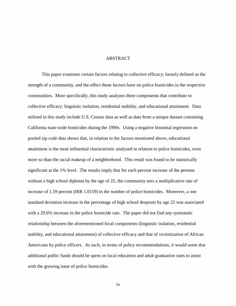
ABSTRACT

This paper examines certain factors relating to collective efficacy; loosely defined as the

strength of a community, and the effect those factors have on police homicides in the respective

communities. More specifically, this study analyzes three components that contribute to

collective efficacy: linguistic isolation, residential stability, and educational attainment. Data

utilized in this study include U.S. Census data as well as data from a unique dataset containing

California state-wide homicides during the 1990s. Using a negative binomial regression on

pooled zip code data shows that, in relation to the factors mentioned above, educational

attainment is the most influential characteristic analyzed in relation to police homicides, even

more so than the racial makeup of a neighborhood. This result was found to be statistically

significant at the 1% level. The results imply that for each percent increase of the persons

without a high school diploma by the age of 25, the community sees a multiplicative rate of

increase of 1.59 percent (IRR 1.0159) in the number of police homicides. Moreover, a one

standard deviation increase in the percentage of high school dropouts by age 25 was associated

with a 29.6% increase in the police homicide rate. The paper did not find any systematic

relationship between the aforementioned focal components (linguistic isolation, residential

stability, and educational attainment) of collective efficacy and that of victimization of African

Americans by police officers. As such, in terms of policy recommendations, it would seem that

additional public funds should be spent on local education and adult graduation rates to assist

with the growing issue of police homicides.

1

CHAPTER I

INTRODUCTION

In recent years politicians and media outlets have portrayed an entrenched battle between

America’s police forces and the neighborhoods they serve. More heightened emphasis has been

placed on the treatment of African American communities in relation to police brutality and, at

extremes, unjustified killings. Examples such as Michael Brown in Ferguson, Freddie Gray in

Baltimore, and Keith Scott in Charlotte have ignited protests and riots, not only in the respective

cities, but across the nation. The civil unrest in these cities, among many others (most recently

Sacramento with Stephon Clark), have put forth a contentious nationwide debate that has not

been experienced with such fervor in decades. The Black Lives Matter movement, with protests

around the country, seems to vilify peace officers due to the perceived targeting of African

Americans and the lack of accountability for these actions. The demonstrations arise from the

strain these communities deal with on a regular basis compounded with the perception of an “us

versus them” mentality towards police officers.

At the extremes of police treatment, police homicides or officer involved shooting deaths

(OISDs) are not extremely uncommon relative to total homicides. Data collected from

California from the 1990s highlight that police “justifiable homicides” accounted for 3.5% of

total homicides. These unfortunate events not only affect communities from a social standpoint,

but also from a financial one. According to data collected from the Los Angeles Times, in the

period spanning 2002 to 2011, taxpayers paid out approximately $101 million to settle lawsuits

2

against Los Angeles Police Department officers accused of wrongful deaths (amongst other

offenses).1 These payouts are not unique to Los Angeles, as other major American cities pay out

hundreds of millions each year in civil suits relating to “justifiable” police homicides. The

community is hurt by loss of life, loss of trust in its police force, and loss of public funds which

could be better served elsewhere. Examining the community factors that play a role in these

deaths may allow municipalities to not only reduce the loss of lives of their respective citizens,

but also save taxpayer dollars on lawsuits and reallocate those funds to other, more beneficial

uses.

Despite the uptick in media coverage and financial strain on cities in relation to OISDs,

the literature regarding police homicides and neighborhood conditions is scarce. While the

rationale behind this discrepancy may be explained by several factors, the primary one is a lack

of systematic and accessible police homicide data. Currently, there is no federal law that

requires incidents of police violence and homicides to be collated in one place. Another limiting

factor is the lack of verifiable victim demographics in relation to the police shootings. The

unique dataset utilized in this paper provides the information necessary to analyze the victim’s

identifiable information and provides the most available granular level of detail of the

neighborhood characteristics involved.

This paper explores the extent that neighborhood factors relating to collective efficacy

and race influence police homicides or OISDs. In this context, collective efficacy refers to

“social cohesion among neighbors combined with their willingness to intervene on behalf of the

common good” (Sampson 1997). The analyses in this paper use a unique datafile of

1 Los Angeles Times, Legal Payouts in LAPD lawsuits. www. http://spreadsheets.latimes.com/lapd-settlements/

(Accessed December 2017).

3

Supplemental Homicide Reports (SHR) compiled by the Federal Bureau of Investigation (FBI),

linked with that of the California Department of Health Services (CDHS) Vital Statistics (VS)

mortality data from the time period 1990 to 1999 for California. For purposes of this paper, the

linked SHR and VS datafile is then combined with available U.S. Census data by ZIP Code. The

U.S. Census data compiled in this analysis relates to the housing and population metrics stored

by the Center for Disease Control and Prevention (CDC). The main goal of this paper is to

isolate key factors relating to the collective efficacy of the neighborhoods that were involved in

OISDs, and their potential effect on police homicides. A secondary aim of this paper is to

investigate the influence of race and the respective neighborhood conditions on OISDs.

This paper is organized as follows. The next chapter frames the issue and provides a

discussion of meaningful literature that has contributed to the issue at hand. Chapter Three

describes in detail the data set used in the analysis. Chapter Four provides the framework of the

negative binomial regression (NBR) methodology employed and the rationale behind that

methodology. Chapter Five provides the results of the NBR analyses with the interpretation of

the results. Lastly, Chapter Six concludes the paper and provides policy suggestions moving

forward.

4

CHAPTER II

LITERATURE REVIEW

Despite the urgent need for more data and research to be published regarding police

treatment in more extreme cases, authorities and municipalities are hesitant to comply with the

publication of such data. Therefore, it has been left up to the public to aggregate police

shootings information, and slowly the data is coming forth. Specifically, the Washington Post

has begun a project to collect specifics of police shootings, beginning with the 2015 year.

Unfortunately, this data is compiled by scanning local newspapers and social media accounts, as

well as by individuals who submit data (and may do so fraudulently to represent a specific

agenda). No systematic, reliable, government sponsored database currently exists to help

analyze the data of police shootings and the community factors that contribute to collective

efficacy of the neighborhoods of the victims.

That being said, prior research does exist that shows that neighborhoods with strong

levels of collective efficacy have lower rates of violence amongst other civilian members of the

community (Sampson 1997). For collective efficacy to develop in a specific community, it is

imperative that community members have valid sentiments of trust and solidarity for others in

the community. Many factors may affect collective efficacy of a neighborhood, but again, the

underlying research shows that when collective efficacy is strong, neighborhoods experience not

only less minor violence and crime, but also less civilian homicides (Wu 2009). Given the stakes

5

at hand, it would seem a worthwhile exercise to link the conditions of neighborhoods with that of

the extreme use of force exhibited by peace officers.

Previous literature, more specifically Sampson and Raudenbush (1999) and Wu (2009),

suggests several at-risk factors as key control variables to examine the community dynamics

within which homicide takes place. The main focal points of collective efficacy put forth by

those papers consist of linguistic isolation, residential stability, and educational attainment by

way of concentrated disadvantage. These aforementioned influences are used as key variables

for this paper, and are explained in more detail below in reference to theories of policing.

In reference to linguistic isolation and policing, this paper proposes two differing

hypotheses which both seem plausible. One is that a more isolated community with respect to

language experience a stronger sense of collective efficacy as they bond over language, and

moreover traditions, which may include sentiments of respect for those in authority. This would

imply less hostility between police officers and the neighborhoods they serve, despite speaking

different languages. Another hypothesis is that officers may seem to have a confrontational or

blatantly racist view to the people they serve that are not of a similar racial makeup to

themselves which allows for a harboring of resentment by the community (Goldkamp 1976).

Furthermore, research has shown that police are less likely to report certain types of crime in

linguistically isolated areas (Varano et al, 2009). These viewpoints and corresponding actions

may increase distrust of police, which could then boil over altercations involving police

homicides.

The second factor of collective efficacy analyzed in this paper is residential stability. The

hypothesis employed is that renters are more likely to be on the move more frequently than that

6

of homeowners, which negatively affects collective efficacy. The positive community benefits

of “laying roots” that home ownership entails has been well documented in relation to residential

stability (Sanbonmatsu et al. 2011; Wood, Turnham and Mills 2008). Police would then be more

familiar with their community members, and be less likely to be involved in an altercation with

known, and involved residents.

The last factor of collective efficacy examined is the notion of educational attainment or

concentrated disadvantage. This concept is that the neighborhoods with poor schooling and the

least educational attainment tend to have not only the lowest incomes but also higher rates of

unemployment, financial dependence, and institutional disinvestment (Freedman & Woods 2013;

Land, et al. 1990; Wilson 1987). As truancy and lack of a desire for educational attainment runs

rampant, investment in property decreases and decay of institutions become commonplace. The

social order then breaks down and the collective efficacy of the neighborhood weakens, allowing

for a harsher tone between the police force and the broken down community it serves.

Racial Differences

Over the past decade, a significant amount of research has been devoted to police

treatment of minorities. The literature has provided many examples of police targeting

minorities for minor infractions to more complex crimes (Engel & Calnon 2004; Jacobs &

O’Brien 1998). The research provides an insight into the mindset of minorities with respect to

their sentiments toward peace officers. Moving forward to a more inclusive society requires

equal treatment of all, especially by those with powers of authority. Jacobs and O’Brien (1998)

showed that cities with more African Americans and, moreover, a recent growth in the African

American population have higher rates of police killings of African Americans. They also found

7

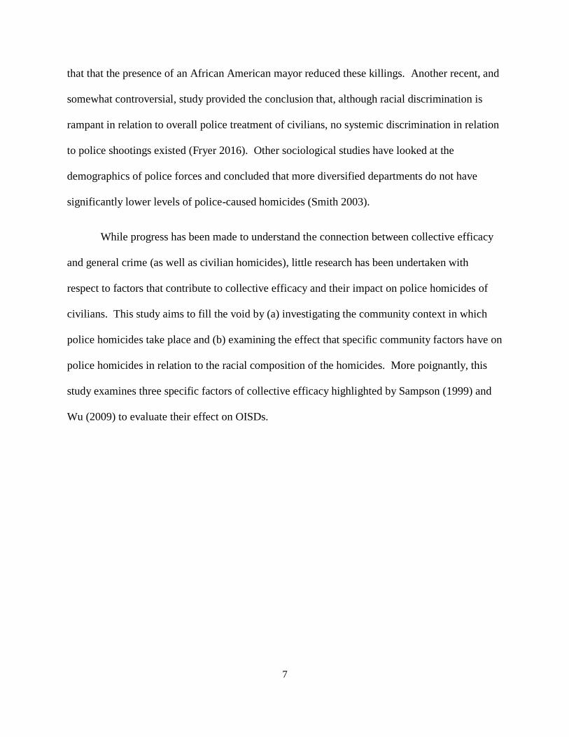
that that the presence of an African American mayor reduced these killings. Another recent, and

somewhat controversial, study provided the conclusion that, although racial discrimination is

rampant in relation to overall police treatment of civilians, no systemic discrimination in relation

to police shootings existed (Fryer 2016). Other sociological studies have looked at the

demographics of police forces and concluded that more diversified departments do not have

significantly lower levels of police-caused homicides (Smith 2003).

While progress has been made to understand the connection between collective efficacy

and general crime (as well as civilian homicides), little research has been undertaken with

respect to factors that contribute to collective efficacy and their impact on police homicides of

civilians. This study aims to fill the void by (a) investigating the community context in which

police homicides take place and (b) examining the effect that specific community factors have on

police homicides in relation to the racial composition of the homicides. More poignantly, this

study examines three specific factors of collective efficacy highlighted by Sampson (1999) and

Wu (2009) to evaluate their effect on OISDs.

8

CHAPTER III

DATA

To date there are very limited systematic data on police homicides along with victim

demographics and details of the incident. Out of the 17,000 law-enforcement agencies in the

United States, only 750, or roughly four percent of the agencies, submitted death-by-police data

to the FBI in the most recent year available. The dataset analyzed in this paper is one of the first

data sources aggregated which contained all homicide data for a particular state, and then broke

out the homicide data by category of homicide. Therefore, the data supplied police homicide

data with accompanying victim demographic information which was matched by two different

agencies.

The homicide data analyzed (ICPSR 3482) contains certain information on victims and

circumstances of the 34,542 homicides investigated by law enforcement agencies in California

for the period 1990 to 1999. The data collection resulted from the project "Linked Homicide File

for 1990-1999," which was conducted by the CDHS, Epidemiology and Prevention for Injury

Control Branch, for the purpose of studying homicide and providing evidence for the

development of strategies to reduce the homicide rate in California. Figure 1 below presents the

homicide rate for California from 1960 through 2011.

9

Figure 1: California Homicide Rate 1960-2011 (Per 100,000 People)2

It is noted that the intention of the linkage project was not to reduce police homicides,

rather the civilian homicide rate. As seen in Figure 1, the homicide rate in California had seen

rates rise throughout the 1970s and remain high in the 1980s, before rising once again in the

early 1990s. Prior to the 1980s, California was routinely toward the middle of all the States in

reference to murder rates. In the 1980s and early 1990s, however, California’s murder rates rose

dramatically, and were consistently in the top 10 of all States.

The specific data are SHRs, which are received monthly by the Department of Justice

from all local California law enforcement agencies as part of the national Uniform Crime

Reporting program (Uniform Crime Reports [United States]: Supplementary Homicide Reports,

2 Data for this figure is collected from the FBI Uniform Crime Annual Crime Reports.

www.disastercenter.com/crime/cacrime.htm. Accessed April 2018.

10

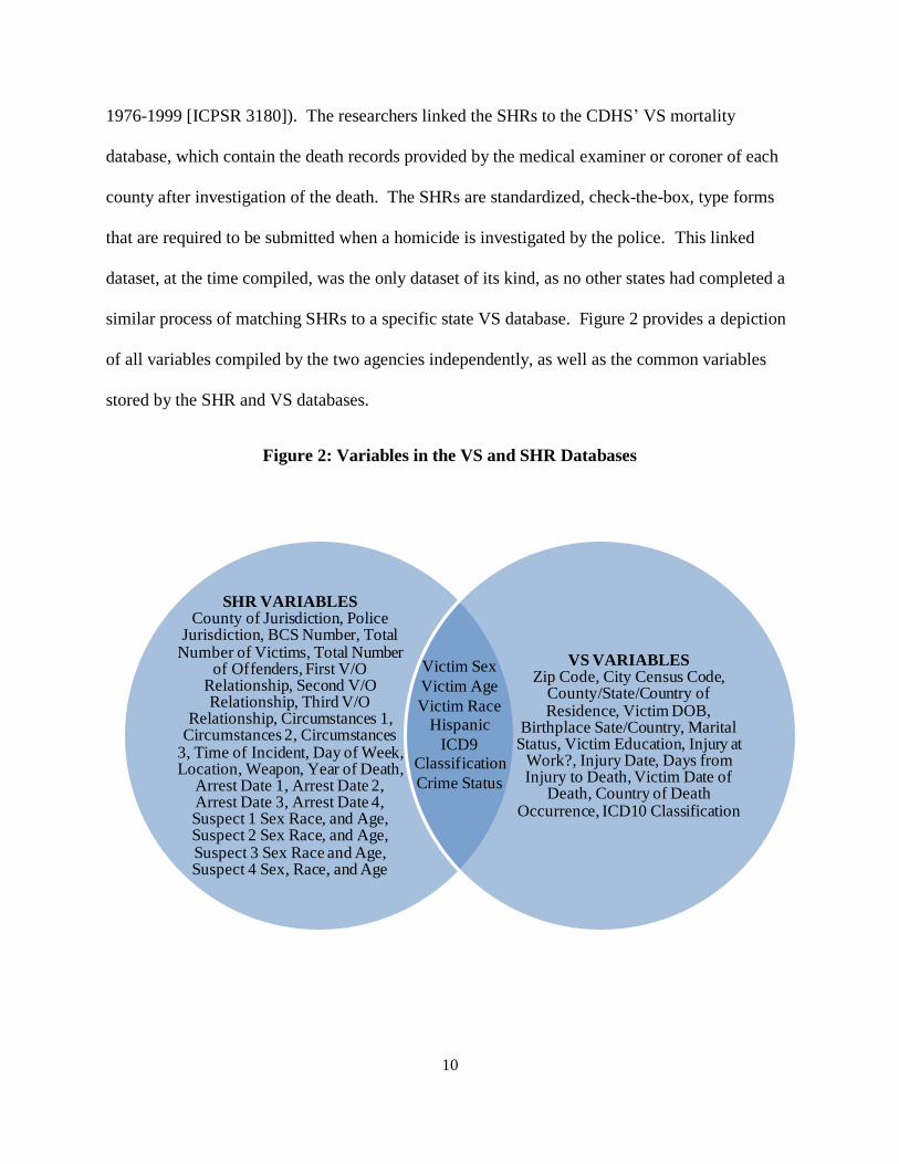
1976-1999 [ICPSR 3180]). The researchers linked the SHRs to the CDHS’ VS mortality

database, which contain the death records provided by the medical examiner or coroner of each

county after investigation of the death. The SHRs are standardized, check-the-box, type forms

that are required to be submitted when a homicide is investigated by the police. This linked

dataset, at the time compiled, was the only dataset of its kind, as no other states had completed a

similar process of matching SHRs to a specific state VS database. Figure 2 provides a depiction

of all variables compiled by the two agencies independently, as well as the common variables

stored by the SHR and VS databases.

Figure 2: Variables in the VS and SHR Databases

SHR VARIABLESCounty of Jurisdiction, Police

Jurisdiction, BCS Number, Total Number of Victims, Total Number

of Offenders, First V/O Relationship, Second V/O Relationship, Third V/O

Relationship, Circumstances 1, Circumstances 2, Circumstances

3, Time of Incident, Day of Week, Location, Weapon, Year of Death,

Arrest Date 1, Arrest Date 2, Arrest Date 3, Arrest Date 4, Suspect 1 Sex Race, and Age, Suspect 2 Sex Race, and Age, Suspect 3 Sex Race and Age, Suspect 4 Sex, Race, and Age

VS VARIABLESZip Code, City Census Code,

County/State/Country of Residence, Victim DOB,

Birthplace Sate/Country, Marital Status, Victim Education, Injury at

Work?, Injury Date, Days from Injury to Death, Victim Date of

Death, Country of Death Occurrence, ICD10 Classification

Victim Sex

Victim Age

Victim RaceHispanic

ICD9 Classification

Crime Status

11

It is of note that SHRs utilize the crime status variable which includes willful homicides,

police and civilian justifiable homicides, and manslaughters. This differs slightly with the VS

database, which uses the International Classification (ICD9) for classifying deaths. The ICD9

has two groupings of relevant homicides: The first is “Homicide and injury purposely inflicted

by other persons” (E960-E969) and the other being “Legal intervention” (E970-E978). Legal

intervention, as noted by Rokaw et al. (1990) include homicides which are “injuries inflicted by

the police or other law-enforcing agents, including military on duty, in the course of arresting or

attempting to arrest lawbreakers, suppressing disturbances, maintaining order, and other legal

action” (p. 449). A review of the data conducted by Riedel and Regoeczi (2006) using a

multilevel analysis comparing on a case-by-case basis found that, indeed, one of the variables

reported with the least amount of agreement was that of police homicides. They found that of

the homicides classified as justifiable by police in the SHR, VS classified roughly half of these

cases as legal intervention homicide. One rationale behind the discrepancy would be that police

compiling SHRs classify more police shootings as justifiable in order to prevent offending

officers from being charged with an offense that carries criminal or civil liability. Another

explanation is that coroners err toward a generic homicide classification than in the lesser used

legal intervention classification. The linked file used in this analysis attempts to merge the two,

and in relation to crime status, the following variables are utilized: criminal homicide, justifiable

– private citizen, manslaughter, and justifiable – peace officer.3 This last option is the basis for

the dependent variable analyzed for the purposes of this paper.

3 Given the data structure, it may be possible that a peace officer could kill someone on duty and it be classified as a

“criminal” homicide or “manslaughter.” However an extensive search yielded no results for such an event for

California in the 1990s. This is not an uncommon trend, as for the ten year period from 2005-2015, only one

California officer was charged with murder or manslaughter in connection with an on-duty shooting.

12

Looking at the homicide data as a whole, we see in the following figure that total

frequency of homicides in the state of California peaks during the 10-year period in 1993 then

steadily declines year over year, reaching a low in 1999. Figure 3 depicts this in a histogram

form covering the years under analysis.

Figure 3: Total Homicides by Year in California 1990-1999

Contrast the above figure with that of the OISDs throughout the 10 year period as

depicted in Figure 4 below.

0.2

.4.6

Den

sity

1990 1991 1992 1993 1994 1995 1996 1997 1998 1999YEAR OF DEATH

13

Figure 4: Total OISDs by Year in California 1990-1999

Similar to total homicides, OISDS peak in 1993, perhaps coinciding with the tensions

around the Rodney King trial and subsequent riots. As opposed to total homicides over the time

frame analyzed, however, OISDs experience another spike in 1997 and trend slightly downward

over the following years. These frequencies suggest that while total homicides decline steadily

over the 1990s, OISDs do not necessarily mirror the overall homicide trend. These initial

statistics and figures allow for a further exploration into the causes of OISDs.

For the purposes of this paper, the homicide data is pooled by zip code to provide a proxy

measure for the community or the neighborhood. Zip code level data is appropriate for the

purposes of this analysis as, practically speaking zip code level data from the U.S. Census was

available to analyze, and the larger geographical regions would distort the “neighborhood” focus

of this paper. Moreover, there is no systematic data that would provide a more granular level of

analysis (e.g. street level, ZIP+4 code). The ability to use a more specified level of geographical

0.1

.2.3

.4

Den

sity

1990 1991 1992 1993 1994 1995 1996 1997 1998 1999YEAR OF DEATH

14

analysis provides particular insight into the communities represented than that of a larger, more

diverse and populated geography. The variables utilized in this analysis are constructed with the

1990 census data. The use of this specific year is primarily due to practicality as the Census is

conducted every ten years, but also to allow for the analysis of data prior to any perceived,

systemic migration due to the tensions around the Rodney King riots and subsequent aftermath.

Two major qualifications are needed when utilizing this dataset, more specifically in

context of police homicides. The first is that the bulk of the data utilized in the analysis is

compiled from reports conducted by the police officers themselves. Inherently there is an

incentive for officers to provide misleading or inaccurate accounts of the homicides in question

so as to not be investigated for any disciplinary actions. Moreover, these reports do not contain

any third -party eyewitness accounts, nor does it contain an account from the victim. It would be

difficult to quantify the misreporting bias associated with the results. Secondly, and perhaps

more obviously, it is nearly impossible to obtain all variables of significance at the time of the

shooting. The SHR data does not go into robust narratives of the circumstances, and act as

solely a form to check whilst investigating a homicide. The user error on these forms, without

misreporting, may indeed be somewhat large, but hard to verify.

In the next section, the paper explores the methodology options available to analyze the

dataset.

15

CHAPTER IV

METHOD

Negative Binomial Regression (NBR) Framework and Selection

The negative binomial regression (NBR) framework is similar to that of the regular

multiple regression with the main exception that the dependent variable is an observed count,

with no natural upper bound, that follows the negative binomial distribution. Therefore, the only

possible values of the dependent variable are positive integers which include zero. The Poisson

framework may be employed if the primary assumption of the mean and the variance of the

respective dependent variables are the same. If not, NBR, is used to correct such a violation (as

put forth by Cameron & Trivedi, 1998).

In negative binomial regression framework, the mean of the dependent variable is

determined by the exposure variable (t) and a set of k regressor variables. The expression relating

these quantities is:

The parameter μ is the mean incidence rate of the dependent variable per unit of

exposure. Exposure may be time, space, distance, area, volume, or population size. The

parameter μ may be interpreted as the risk of a new occurrence of the event during a specified

exposure period. The NBR is a generalization of Poisson regression which releases the limiting

16

assumption that the variance is equal to the mean. The NBR model adds a parameter that allows

the conditional variance of the dependent variable to exceed the conditional mean.

The use of the NBR, instead of the commonly used ordinary least squares (OLS)

regression, is based on the following characteristics of the data. First, police homicide is a rare

event relative to total homicides. To construct a police homicide rate based on rarity would

make the dependent variable unstable. Second, a prognosis test detects an overdispersion in the

dependent variables which means, the mean and variances of the dependent variables utilized in

this analysis, specifically OISDs and race-specific OISDs, are not equal. This overdispersion is

caused by the skewed nature of the dependent variable, namely, OISDs. Graphically, it is

apparent that all the dependent variables analyzed in the models employ do not follow a normal

distribution, and more specifically, overdispersion occurs in each case. The appendix provides

histograms of all dependent variables analyzed in this paper. Lastly, since the dependent

variable contains several zero values, a zero-inflated negative binomial model (ZINB) may be of

use in the analysis.4 However, there are two assumptions as to why the NBR is the preferred

methodology. One, the excess zeros cannot be modeled independently, as there are not two

possible processes that arrive at a zero outcome. That rationale relies on the assumption that

police officers are not providing false statements on SHRs. Secondly, when performing a test

similar to Vuong (1989), the z-value of that analysis is not significant which highlights that the

ZINB is not a better fit that the standard NBR. The Vuong closeness test uses the Kullback-

Leiber Information Criterion to measure the goodness of fit for two models. This test can be

used to determine whether zero-inflation is present in data. For these reasons, for the purposes of

4 In relation to the number of dependent variable zeros, there were 1,024 out of 1,523 California zip codes that did

not experience an OISD during the 1990s.

17

this analysis, the NBR provides the more reliable framework than that of other models including

a more generic Poisson estimation, a modified OLS regression, or a ZINB framework.

Specific NBR Model Defined

The form of the model equation for NBR is identical to that of the Poisson regression in

as such the log of the outcome is predicted with a linear combination of the predictors. In this

instance, the primary NBR empirical model estimated is the following:

, (1)

which implies:

In performing the analysis, both NB1 and NB2 variances were conducted, and the more standard

NB2 model was utilized. The results did not differ significantly with this methodology.

Dependent Variable

OISDs is the pooled count of police homicides for each of the 1,523 zip codes in

California throughout the 1990s. In reference to the specific dataset, a police homicide or OISD

is coded as “peace officer – justifiable.” As the number of police homicides is relatively

uncommon compared to that of other homicides (roughly 3.5 percent of all homicides during the

time period analyzed), a pooled count of police homicides from 1990 to 1999 is the more

appropriate measure to utilize. This methodology ensures a sufficient count for multivariate

analysis. The aggregation of police homicides by zip code area is further extrapolated to

generate pools of OISDs for by race (African American versus non-African American) in order

18

to carry out race-specific specifications. The use of zip code area in this study is a pragmatic

choice as the dataset is broken down to zip code level data. Furthermore, previous literature

suggests that studies which employ metropolitan areas, counties, and zip code level data show

findings which tend to converge among other studies which use macrounits of analysis (Lee &

Bartkowski, 2004).

Explanatory Variables

Similar to analyses conducted by Wu (2009), this paper looks at factors of collective

efficacy and its relation to homicide. Deviating from Wu, this paper (i) does not aggregate the

factors into a combined index for collective efficacy, and (ii) focuses on a unique subset of

homicide data (OISDs). The analyses provided in this paper aim to isolate the specific factors

relating to collective efficacy that provide the most impact to OISDs. Employing indices of

multiple variables as a proxy for collective efficacy may distort the individual components,

which this paper attempts to correct. This paper uses proxy percentages for key factors of

collective efficacy highlighted by Sampson and Raudenbush (1999) and Wu (2009): More

specifically, for linguistic isolation, the variable used is the percent of linguistic isolation in a

community. For the purposes of data collection from the CDC, and moreover this analysis, the

linguistic isolation variable is computed as the summation of households that speak only

Spanish, an Asian/Pacific language, or other non-English language divided by that of the total

population of the zip code. For residential stability, the variable is computed as renter occupied

percentage of occupied housing over total occupied housing of the zip code. Lastly, in reference

to educational attainment, the calculation for the proxy for this variable is the number of adults

under 25 years of age without a high school diploma divided by total persons of a zip code. Each

of these variables were calculated from 1990 U.S. Census data at the zip code level.

19

Other control variables that are of interest and therefore entered into the framework are

single mother households, home age in a community, the median home prices, and the median

household income. Each of these control variables were analyzed to provide a more robust

analysis. Finally, neighborhood civilian killings may be a large factor on whether or not an

officer uses excessive force to resolve an altercation. To provide some methodology controlling

for prior sources of crime/local homicides, a lagged variable based on total homicide count in

each zip code for 1990 was constructed and employed as a control variable.

Racial Differences Specifications

As mentioned in the introduction of this paper, the focal point for media outlets and

politicians have been the police homicides of the African American community. As such, it is

important to delineate between African American victims of OISDs and the rest of the

population of OISDs. Therefore, two additional specifications are employed to be able to

provide for this analysis:

, (2)

(3)

The control variables in (2) and (3) above remain similar to that of equation (1), however, the

dependent variables analyzed in these alternate specifications are OISDs in which the victim was

African American (2), and OISDs where the victim was not identified as African American (3).

Exposure Issue

Count models, such as the NBR model, require a mechanism to deal with the fact that

counts can be made over different observation periods. Count models account for these

20

differences by including the log of the exposure variable in model with coefficient constrained to

be one. In this instance, the count of OISDs by way of pooled zip codes are utilized as

dependent variables for the various specifications presented. The population of each zip code

may influence the number of OISDs in a given zip code. A higher population zip code, say one

with a million people, will most likely have more OISDs than that with 100 people. To account

for this issue, the population of each zip code is used as an offset or exposure variable. While

the use of exposure variables is, in many cases, superior to that of analyzing rates (or per capita)

measures as control variables, the Appendix provides the results of the analysis removing

population as an exposure variable, and inserting it as a control variable. The rationale behind

using population as an offset variable instead of a control variable is due to the fact that it makes

use of the correct probability distributions for the NBR model employed. Regardless of the

model employed, the results of the analyses do not significantly change.

Multicollinearity Issue

Previous studies involving aggregate data have suggested that some independent

variables in the analytical model tend to have a high degree of correlation that causes a

multicollinearity problem. For the purposes of this analysis, to circumvent the issues caused by

the multicollinearity problem, an ordinary least squares regression is employed to the models to

obtain the variance inflation factors (VIFs). There are varying opinions around thresholds for

VIFs and rejecting independent variables (see O’Brien, 2007). Following Marquardt (1970) and

Hair et al (1995), variables that produced variance inflation factors scores greater than 10 were

removed from the analysis as these variables pose the potential problem of multicollinearity. No

variable in the analysis exceeds the threshold suggested by these studies. All control variables

21

had VIFs under 3.0. It is also noted that the mean VIF for all the specifications highlighted in

the next section are under the 2.5 threshold (1.93) suggested by Allison (1999).

22

CHAPTER V

RESULTS

There were 34,542 victims of homicides California-wide during the ten-year period

ranging from 1990 through 1999. OISDs accounted for approximately 3.5% (N=1,204) of total

cases. Table 1 presents the results of the statewide breakdown of homicide cases separating into

two distinct groupings: OISDs and non-OISDs, other relevant victim background demographics.5

5 It is noted that OISDs do not include civilian killings of police officers, for the purposes of this exercise these

events are grouped into non-OISDs

Table 1: Victim Background Factors- OISDs versus Non-OISDs

OISDs Non-OISDs

% (N) % (N)

State-wide (1) 3.5 (1,204) 96.5 (33,338)

Sex

Male 97.8 (1,178) 81.6 (27,220)

Female 2.2 (26) 18.4 (6,118)

Race

Black 21.8 (261) 28.0 (11,385)

Hispanic 36.7 (440) 42.8 (14,211)

Non-Black, Non-Hispanic 39.4 (497) 29.1 (7,742)

In Years (N) In Years (N)

Age 31.0 (1,192) 30.0 (32,921)

Black 28.2 (260) 29.1 (9,252)

Non-Black 31.8 (932) 30.3 (23,669)

Education 14.3 (1,141) 13.4 (30,981)

Black 15.0 (251) 13.2 (8,901)

Non-Black 14.2 (890) 13.4 (22,080)

(1) Due to missing data, certain subtotals do not add up to total observations.

23

Men were the overwhelming majority of these victims accounting for 97.8% of the

homicide cases. Contrast that with non-OISDs where women make up roughly 18.4% of the

victims.

In reference to non-police homicides during this time period, on average, approximately

28% of the victims were African American, 43% were Hispanic, and 29% were non-African

American, non-Hispanic (white). Contrast these statistics with the OISDs, and we find that 22%

of OISDs in our data were African American, 37% were Hispanic, and roughly 40% were white.

These summary statistics yield a surprising result: the percentage of African American victim

homicides decreases by nearly seven percent when looking at the non-OISD population of

homicides compared to that of OISDs. Keeping that in mind, from the data we see that African

American victims of OISDs are slightly younger on average than that of non-officer involved

fatalities.

Table 2 presents the grouped zip code level measurements utilized in the multivariate

analysis. Of the total of 1,523 zip codes in California, roughly 30% (N=499) recorded at least

one OISD. Moreover, roughly 8% (N=127) recorded at least one OISD involving a African

American victim. 6

6 Roughly 9.7 (N=3,345) percent of the total number of homicides occurred outside of the county of residence. Only

12 of these homicides were OISDs, with all but one being Mexican nationals with place of death in California.

Therefore it is assumed that zip code of residence is not distinctively different from zip code of event for purposes of

analysis.

24

The statistics above show that the variance of the dependent variables analyzed in the

specifications employed, namely total OISDs, African American OISDs, and non-African

American OISDs exceed that of the mean. The summary statistics also highlight that on average,

less than one (0.685) police homicide occurred per zip code in the 1990s. As mentioned in the

methodology section of this paper, this assumption is a necessary requirement for usage of the

NBR methodology.

NBR Results

NBR is applied to the following three models of analysis: all OISDs cases, African

American victim cases, and non-African American victim instances. The first model tests the

primary factors of collective efficacy on total police homicides with that to see the merits of

each. The second and third specifications follow a similar structure, but instead focus on the

racial context of the collective efficacy factors and their applicability to OISDs by comparing

African Americans versus that of the cases with non-African American victims.

Table 2: Summary Statistics for Grouped Zip Code Level Variables (N=1,523)

Variables Mean Std. Dev.

Total OISDs 0.685 1.355

Black victim OISDs 0.156 0.668

Non-Black victim OISDs 0.529 1.039

Race: Black (Percent) 4.727 10.072

Race: Non-Black (Percent) 95.273 10.072

Linguistically isolated (Percent) 6.066 8.046

Renters (Percent) 39.718 20.108

Non high school graduate under 25 (Percent) 23.758 16.425

Female head of household (Percent) 12.131 11.508

Home older than 1950 (Percent) 20.915 18.421

Homicide 1990 0.590 3.921

Median income in 1989 34,576 14,983

Median home value in 1990 179,052 118,974

Population in 1990 19,540 19,126

25

Table 3 shows the results of the NBR for all police homicide cases aggregated by

California zip codes over the 10-year period. The figures in the first column of the table

presented are the NBR coefficients, with robust standard errors highlighted in the parentheses

underneath that of the coefficients. The second column highlights the estimated incidence rate

ratios (IRR) for the variables analyzed. The IRR is the estimated rate ratio for a one unit

increase in a variable, given the other variables are held constant in the model. In order to

estimate the magnitude of each significant predictor in terms of percentage change in the

dependent variable, a transformation is necessary. Moreover, the following formula is used in

accordance with the transformation provided in equation (1) of the methodology section to

estimate the effect on the dependent variable of a one standard deviation change in a control

variable:

*100 (4)

whereas, b is the NBR coefficient associated with the kth control variable, and s b is the standard

deviation associated with the kth control variable.

26

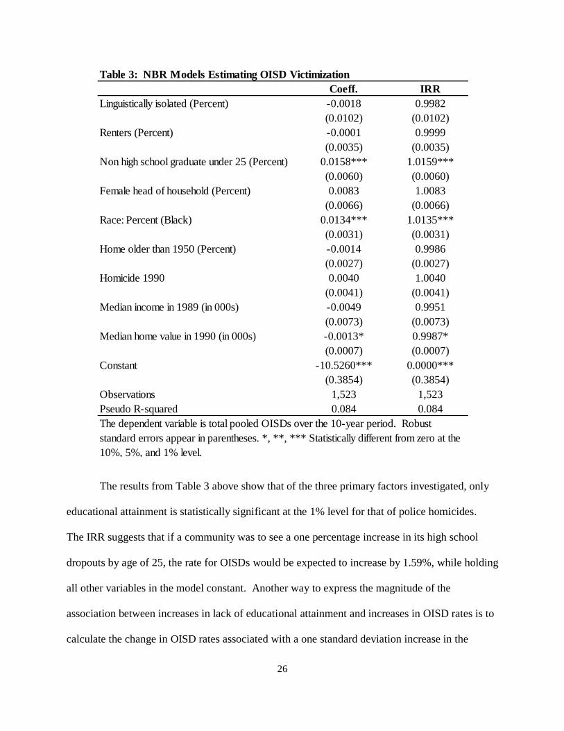
The results from Table 3 above show that of the three primary factors investigated, only

educational attainment is statistically significant at the 1% level for that of police homicides.

The IRR suggests that if a community was to see a one percentage increase in its high school

dropouts by age of 25, the rate for OISDs would be expected to increase by 1.59%, while holding

all other variables in the model constant. Another way to express the magnitude of the

association between increases in lack of educational attainment and increases in OISD rates is to

calculate the change in OISD rates associated with a one standard deviation increase in the

Table 3: NBR Models Estimating OISD Victimization

Coeff. IRR

Linguistically isolated (Percent) -0.0018 0.9982

(0.0102) (0.0102)

Renters (Percent) -0.0001 0.9999

(0.0035) (0.0035)

Non high school graduate under 25 (Percent) 0.0158*** 1.0159***

(0.0060) (0.0060)

Female head of household (Percent) 0.0083 1.0083

(0.0066) (0.0066)

Race: Percent (Black) 0.0134*** 1.0135***

(0.0031) (0.0031)

Home older than 1950 (Percent) -0.0014 0.9986

(0.0027) (0.0027)

Homicide 1990 0.0040 1.0040

(0.0041) (0.0041)

Median income in 1989 (in 000s) -0.0049 0.9951

(0.0073) (0.0073)

Median home value in 1990 (in 000s) -0.0013* 0.9987*

(0.0007) (0.0007)

Constant -10.5260*** 0.0000***

(0.3854) (0.3854)

Observations 1,523 1,523

Pseudo R-squared 0.084 0.084

The dependent variable is total pooled OISDs over the 10-year period. Robust

standard errors appear in parentheses. *, **, *** Statistically different from zero at the

10%, 5%, and 1% level.

27

percentage of persons without a high school diploma by the age of 25 (SD = 16.4%). In the

primary model, after utilizing the transformation provided in equation (4), a one standard

deviation increase in the percentage of high school dropouts by age 25 was associated with a

29.6% increase in the OISD rate. Also statistically significant at the 1% level in terms of

estimating OISDs is the percentage of the community that is African American. The results

suggest that a 1% increase in the percentage in the African American contingent of a community

results in an increase in the OISD rate by 1.43%.

While not statistically significant, the results show that the more linguistically isolated a

community is the less police homicides occur in that respective neighborhood. The direction of

the coefficient may be due to the fact that non-English speaking communities are more respectful

of police officers, and therefore are less likely to become combative with peace officers. It also

may be due to the fact that California has maintained, and continues to maintain, a relatively high

level of Latino police officers. The assumption here is the Latino citizens and Latino police

officers share a language, and moreover a cultural background, which facilitates a more

harmonious community. This result mirrors that of Varano (2009) in studying police behavior

with respect to minority communities in San Antonio, Texas. The residential stability variable

provides the least impact by magnitude, and is also not statistically significant. The rationale

behind the lack of significance of the linguistic isolation and residential stability variables may

be due to the diverse nature of zip codes in California. Each individual zip code may harbor

more than one community, and conversely, one singular community may be located in several

zip codes. The lack of precise location of OISDs, and defaulting on zip codes may not provide

the level of granularity to achieve statistical significance with respect to these variables.

28

Racial Differences

In reference to the racial discrepancies of OISDs, Table 4 presents the two specifications

regarding race. The first column highlights the estimation of OISDs in which the victim was

African American, and the second column estimates the remainder of OISD victimization (or

non-African American). The purpose of this analysis is to examine if any racial difference exists

in relation to the collective efficacy factors and their respective effects on race-specific

homicides committed by peace officers.

29

From Table 4 above, we see that none of the primary factors of collective efficacy

analyzed in this paper are statistically significant in predicting African American OISDs. While

not statistically significant, educational attainment for African Americans have the largest

magnitude with respect to all other analyzed variables. This corroborates the primary analysis.

On the other hand, for non-African Americans, educational attainment is statistically significant

at the 1% level similar to that of total OISDs. Another statistically significant variable with

Table 4: NBR Models Estimating Black and non-Black OISD Victimization

Black Non-Black

(1) (2)

Linguistically isolated (Percent) -0.0017 -0.0045

(0.0182) (0.0115)

Renters (Percent) 0.0109 0.0006

(0.0067) (0.0039)

Non high school graduate under 25 (Percent) 0.0147 0.0178***

(0.0134) (0.0066)

Female head of household (Percent) -0.0029 0.0136*

(0.0135) (0.0075)

Race: Percent (Black) 0.0479*** -0.0115**

(0.0062) (0.0047)

Home older than 1950 (Percent) 0.0072 -0.0049

(0.0065) (0.0030)

Homicide 1990 0.0020 0.0056

(0.0069) (0.0047)

Median income in 1989 (in 000s) 0.0079 -0.0055

(0.0178) (0.0078)

Median home value in 1990 (in 000s) -0.0023 -0.0011

(0.0014) (0.0008)

Constant -13.4618*** -10.6347***

(0.9522) (0.4192)

Observations 1,523 1,523

Pseudo R-squared 0.204 0.053

The dependent variable in (1) is total pooled OISDs in which the victim was black over the 10-year

period. The dependent variable in (2) is total pooled OISDs in which the victim was not black over

the 10-year period. Robust standard errors appear in parentheses. *, **, *** Statistically different

from zero at the 10%, 5%, and 1% level.

30

respect to non-African Americans, albeit at the 10% level, is the female head of household

variable.

Overall these results are somewhat surprising, as they confirm that while the racial

makeup of a community does play a role in the level of OISDs for that specific neighborhood,

there is no statistically significant systematic relationship between the key components of

collective efficacy and that of victimization of African Americans by police officers. Further

research and data collection is warranted to provide for a more complete explanation.

Specifically, a more complete database of police shootings which include the exact location of

incident and more robust officer/victim demographics would prove to be fruitful. Additionally, a

more direct measure of collective efficacy, as opposed to indirect proxies of key factors, would

be instrumental to subsequent analyses. Without direct evidence reported by residents covering

several communities, as is the case with Kochel (2011) who surveyed residents of Trinidad and

Tobago, such a proxy measurement remains imperfect. Future efforts could incorporate both (i)

a more robust and precise police shooting database, and (ii) a direct measure of collective

efficacy of a large number of reflective communities.

31

CHAPTER VI

CONCLUSION

Police shootings have dominated media outlets over the past several years and have

incited a discourse amongst the American people. This topic is one that continues to polarize the

nation and continues to elicit a combative tone which, at the most extreme, can result in riots and

violence. Surprisingly, there has not been a large, municipality-by-municipality sponsored effort

to collect data to examine racial disparities in police shootings combined with community

factors. This data may alleviate the burden placed on police officers so that they may uphold the

law without fear of unwarranted retribution. The data may also allow for a look into any

systematic abuses of police and warrant policy changes in accordance with those infractions.

The fact that embedded in the data may be a component of misreporting by way of

“protecting the shield” is a key issue. As the dependent variable is taken as granted by way of

the police self-reporting the unraveling of the event at hand, there is a strong possibility that the

dependent variable suffers from misreporting bias. While unlikely, it may be the case that police

officers alter the facts to make it seem that the event was not an OISD, but rather a case of

civilian homicide. Therefore, it is quite impossible to know how widespread this type of

misreporting bias is (Schneider, 1977). This misrepresentation of events can be systematically

reduced by way of objective viewpoints from that of the officers themselves. Taking away the

subjectivity of the events requires first hand visual and audio evidence. Specifically, police body

cameras have been enacted in several jurisdictions throughout the country, and can assist with

32

holding officers accountable in extreme situations or exonerating them from any wrongdoing.

While the body cameras and dashboard video that provide distinct visual evidence are not

uncommon these days, the collection and dissemination of the data will take years to effectively

collect and analyze.

Speaking directly to the results of this paper, the analysis shows that community leaders,

police, policymakers, elected officials and other stakeholders should focus their efforts on

educational attainment for its citizens in order to potentially reduce police homicide. The results

of the primary analysis suggest for every 1% increase in the population of a community lacking a

high school diploma by age 25, the rate of OISDs increases by 1.59%. Furthermore, a one

standard deviation increase in the percentage of high school dropouts by age 25 was associated

with a 29.6% increase in the OISD rate The theory being that an educated and invested citizen is

one that is not only more likely to remove him or herself from a position of concentrated

disadvantage, but also less likely to engage in criminal activity and therefore have an altercation

with the police that ends in tragedy. The results echo findings by Kochel (2011) who examined

the island nation of Trinidad and Tobago and found a relationship between quality routine police

services, levels of police misconduct, and collective efficacy. In Trinidad, the amount and nature

of interactions with police appear to play an important part in residents’ and neighborhood‐level

assessments about police services and misbehavior.

A potential tool that may allow for the desired outcome of less police homicides is the

‘beat meeting’ – regularly scheduled meetings of the police with residents of their respective

beats they patrol. Beat meetings would be best served at local schools with police interacting

with community members including school age children. This would allow for a certain trust of

peace officers from community members at a young age, and may assist with graduation rates.

33

These meetings can be of particular importance in communities that are predominately African

American. While the paper does not find any systematic relationship between the linguistic

isolation, residential stability, or concentrated disadvantage of a community and that of

victimization of African Americans by police officers, it does find a statistically significant result

for African American population and local OISDs. Funding for these types of programs which

allow for police and community members to interact and to promote educational attainment

would seem to be a more worthwhile endeavor than funding for police misconduct lawsuits. A

stronger, more together neighborhood involves determined efforts by both its civilian members

and its police officers.

34

REFERENCES

Allison, P. (1999). Multiple Regression: A Primer. Thousand Oaks, California: Pine Forge Press.

Bui, Q. and Cox, A. (2016, July 11). Surprising New Evidence Shows Bias in Police Use of

Force but Not in Shootings. New York Times. Retrieved from http://www.nytimes.com.

Cameron, A. C., & Trivedi, P. K. (1998). Regression Analysis of Count Data. Cambridge, UK:

Cambridge University Press.

Cameron, A. C., & Trivedi, P. K. (2013). Regression Analysis of Count Data, 2nd edition.

Econometric Society Monograph No.53, Cambridge University Press, 1998.

Engel, R. & Calnon, J. (2004). Examining the Influence of Drivers’ Characteristics During

Traffic Stops with Police: Results from a National Survey. Justice Quarterly, 21(1).

Fryer Jr., R. (2016). An Empirical Analysis of Racial Differences in Police Use of Force.

National Bureau of Economic Research Working Paper Series. Working Paper 22399.

Dupont, W. D. (2002). Statistical Modeling for Biomedical Researchers: A Simple Introduction

to the Analysis of Complex Data. New York: Cambridge Press.

Freedman, D., & Woods, G. W. (2013). Neighborhood Effects, Mental Illness and Criminal

Behavior: A Review. Journal of Politics and Law, 6(3), p.1–16.

Goldkamp JS. (1976). Minorities as victims of police shootings: Interpretations of racial

disproportionality and police use of deadly force. The Justice System Journal. 2(2), p.

169–183.

Hagan, J. and Peterson R, eds. (1995). Crime and Inequality. Stanford, Calif.: Stanford

University Press.

Hilbe, J. (2013). Negative Binomial Regression: 2nd edition. Cambridge, United Kingdom.

Cambridge University Press.

Hair, J. et al. (1995). Multivariate data analysis: with readings. Englewood Cliffs, New Jersey,

Prentice-Hall.

Jacobs D. (1998) The Determinants of Deadly Force: A Structural Analysis of Police Violence.

American Journal of Sociology. 103(4), p.837–862.

35

Land, K. et al. (1990). Structural Covariates of Homicide Rates: Are There Any Invariances

across Time and Space? American Journal of Sociology. 95(4), p.922–63.

Lee, M. and Bartowski, J. (2004). Civic Participation, Regional Subcultures, and Violence: The

Differential Effects of Secular and Religious Participation on Adult and Juvenile

Homicide. Homicide Studies. 8(1), p.5-39.

Long, J. S. (1997). Regression Models for Categorical and Limited Dependent Variables.

Thousand Oaks, CA: Sage Publications.

Marquardt, D. (1970). Generalized Inverses, Ridge Regression, Biased Linear Estimation, and

Nonlinear Estimation. Technometrics. 12(3), p.591-612.

Rokaw, W. M., Mercy, J. A., & Smith, J. C. (1990). Comparing Death Certificate Data with FBI

Crime Reporting Statistics on U.S. Homicides. Public Health Reports. 105, p.447-455.

Sampson, R. and Raudenbush, S. (1997). Neighborhoods and Violent Crime: A Multilevel Study

of Collective Efficacy. Science. 277(5328), p.918-924.

Sampson, R. and Raudenbush, S. (1999). Systematic Social Observation of Public Spaces: A

New Look at Disorder in Urban Neighborhoods. American Journal of Sociology. 105(3),

p.603-651.

Sanbonmatsu, L. et al. (2011). Moving to Opportunity for Fair Housing Demonstration Program

-Final Impacts Evaluation. Prepared for the U.S. Department of Housing and Urban

Development, Office of Policy Development & Research. Retrieved from:

http://www.huduser.org/publications/pdf/MTOFHD_fullreport.pdf.

Schneider, A., (1977). Portland (Or) Forward Record Check of Crime-Victims Final Report,

Oregon Research Institute and United States of America. December 1977.

Smith, B. (2003). The Impact of Police Officer Diversity on Police-Caused Homicides. Policy

Studies Journal. 31(2), p.147-162.

Van Court, J. (2006). CALIFORNIA VITAL STATISTICS AND HOMICIDE DATA, 1990-

1999 [Computer file]. ICPSR03482-v2. California Dept. of Health Services,

Epidemiology and Prevention for Injury Control Branch, Violent Injury Surveillance

Program. Sacramento, CA.

Varano, S. et al. (2009). Constructing Crime: Neighborhood Characteristics and Police

Recording Behavior. Journal of Criminal Justice. 37(2009), p.553-563.

Vuong, Q. (1989). Likelihood Ratio Tests for Model Selection and non-nested Hypotheses.

Econometrica. 57(2), p.307–333.

Wilson, W. (1987). The Truly Disadvantaged: The Inner City, the Underclass, and Public

Policy. Chicago: University of Chicago Press.

Wood, M, et al. (2008). Housing Affordability and Family Well-Being: Results from the

Housing Voucher Evaluation. Housing Policy Debate. 19(2), p.367-412.

36

Wu, B. (2009). Intimate Homicide Between Asians and Non-Asians: The Impact of Community

Context. Journal of Interpersonal Violence. 24(7).

APPENDIX

38

Appendix Figure A1: Histogram of Total OISDs

Appendix Figure A2: Histogram of Total Non-OISDs

0.5

11.5

2

Den

sity

0 2 4 6 8 10OISDS

0

.01

.02

.03

.04

.05

Den

sity

0 100 200 300 400 500NONOISDHOM

39

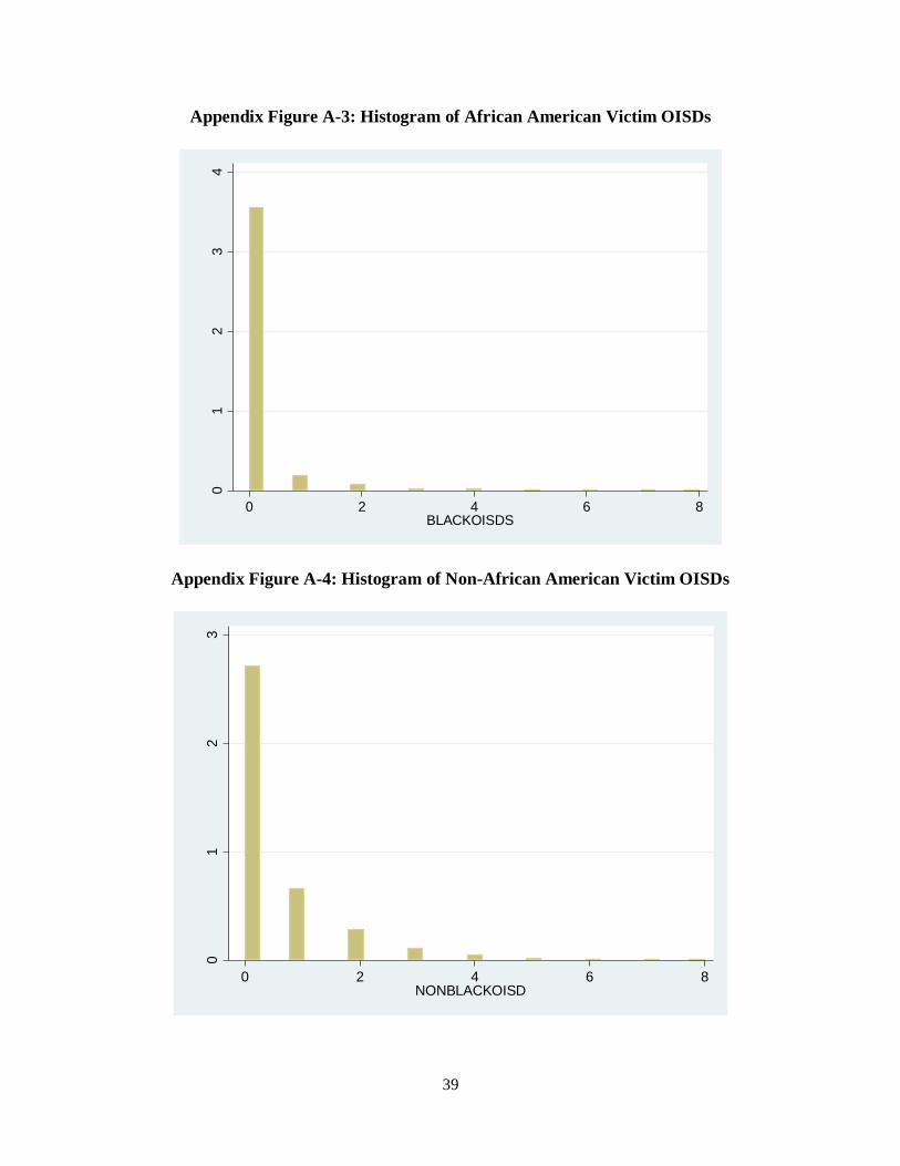
Appendix Figure A-3: Histogram of African American Victim OISDs

Appendix Figure A-4: Histogram of Non-African American Victim OISDs

01

23

4

Den

sity

0 2 4 6 8BLACKOISDS

01

23

Den

sity

0 2 4 6 8NONBLACKOISD

40

Appendix Table B-1: Alternate Analysis Using Population as Control Variable

OISDs (1)

BLACK OISDS

(2)

NON-BLACK

OISDS (3)

Linguistically isolated (Percent) 0.0044 0.0054 0.0032

(0.0083) (0.0162) (0.0090)

Renters (Percent) 0.0026 0.0096* 0.0037

(0.0027) (0.0056) (0.0030)

Non high school graduate under 25 (Percent) 0.0112** 0.0068 0.0185***

(0.0044) (0.0115) (0.0039)

Female head of household (Percent) 0.0168*** 0.0105 -0.0033

(0.0037) (0.0098) (0.0043)

Race: Percent (Black) 0.0202*** 0.0547*** -0.0075**

(0.0029) (0.0057) (0.0030)

Home older than 1950 (Percent) -0.0042 0.0055 0.0123***

(0.0028) (0.0065) (0.0047)

Homicide 1990 -0.0064 -0.0092 -0.0082

(0.0071) (0.0095) (0.0075)

Median income in 1989 (in 000s) 0.0006 0.0056 -0.0002

(0.0050) (0.0134) (0.0052)

Median home value in 1990 (in 000s) -0.0005 -0.0011 -0.0004

(0.0006) (0.0012) (0.0006)

Population (in 000s) 0.0449*** 0.0453*** 0.0449***

(0.0021) (0.0044) (0.0022)

Constant -2.4442*** -5.0521*** -2.4900***

(0.2546) (0.6883) (0.2673)

Observations 1,523 1,523 1,523

Pseudo R-squared 0.228 0.288 0.207

The dependent variable in (1) is total pooled OISDs over the 10-year period. The dependent variable in (2) is

total pooled OISDs in which the victim was black over the 10-year period. The dependent variable in (3) is

total pooled OISDs in which the victim was not black over the 10-year period. Robust standard errors appear

in parentheses. *, **, *** Statistically different from zero at the 10%, 5%, and 1% level.