Collection of Papers in commemoration of Prof. de Waal’s

34 years of service as the Head of Department of

Mathematical Statistics

Most of the recent research by Prof. Daan de Waal was devoted to extreme value

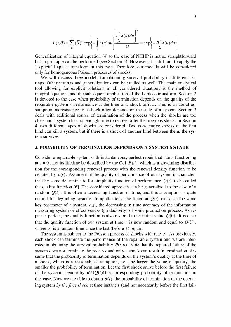
theory and its applications. However, he himself has created data for future

researchers in this area. Indeed, 34 years of service to the Department as its Head is a

remarkable extreme value!

In this volume, his friends and colleagues present some of their latest research. The

first contribution “About Daan” combines experiences, memories and biographical

facts.

Contents

Crowther, N., Finkelstein, M., Groenewald, P., van der Merwe, A., Nel, D., Verster,

A., and de Wet, T . About Daan....................................................................................2

Van der Merwe, A., and Chikobvu, D. Control chart for the sample variance based on

its predictive distribution……………………………………………………………..13

Finkelstein, M., and Marais, F. On terminating Poisson processes in some shock

models………………………………………………………………………………..22

Verster, A., and de Waal, D. Investigating approximations and parameter estimation

of the Multivariate Generalized Burr-Gamma distribution…………………………..33

De Wet, T. Semi-parametric inference for measures of inequality…………………..62

Von Maltitz, M., and van der Merwe, A. An application of sequential regression

multiple imputation on panel data……………………………………………………71

Van der Merwe, S. Time series analysis of the southern oscillation index using

Bayesian Additive Regression Trees…………………………………………………90

Beirlant, J., Dierckx, G., and Guillou, A. Biased reduced estimators in joint tail

modelling……………………………………………………………………………..99

Crowther, N. A simple estimation procedure for categorical data analysis………...114

Schall, R., and Ring, A. Statistical characterization of QT prolongation …...........119

Nel, D., and Viljoen, H. Some aspects of common singular spectrum analysis and

cointegration of time series…………………………………………………………151

2

D.J. (Daan) de Waal

Daan de Waal attended school in the town of Boshoff in the Free State. His intention had

always been to take up farming on the family farm in the district after leaving school, that

is, until a teacher advised him to study for a degree in agriculture at the newly established

Faculty of Agriculture at the University of the Orange Free State. It was then decided that

Daan would study for the four-year BSc Agric degree , hopefully to equip him better for a

successful farming career. Arriving at the university at the beginning of 1959 Daan had no

idea which subjects to enrol for. On learning that his best subject at school was

mathematics, the then dean of the faculty, Prof. R. Saunders, enrolled him with Biometry

and Statistics as majors. Prof. Saunders was a biometrician himself and had written a

textbook, “Experimental Design”, with Prof. A.A. Rayner of the University of Natal,

Pietermaritzburg. So now Daan was enrolled for a degree in agriculture, but with majors

he had never heard of.

However, after four years of study he was hooked and decided to continue with an

honours degree and finally with an MSc Agric in Biometry/Statistics, which he obtained

with distinction in 1964. During his post graduate studies at the Faculty of Agriculture,

Daan also lectured Biometry II and Biometry III, among others to Hennie Groeneveld who

later became Professor in Biometry and Statistics at the University of Pretoria. By now the

idea of a farming career had gone out of the window and in 1965 Daan was appointed as

lecturer in the Department of Statistics of the UOFS, where Prof. Andries Reitsma was

head with Koos Oosthuizen as senior lecturer. During this time statistics was the new

buzzword in mathematical sciences and statistics departments were created and growing at

universities all over the country.

Daan developed an interest in multivariate analysis, largely influenced by the 1958

textbook of T.W. Anderson, which was considered the definitive work on that subject at

the time. He wanted to continue with his PhD studies in that field and was advised by

Prof. Dries Reitsma to contact Prof. Cas Troskie at UCT. Cas was the newly appointed

head of the Statistics Department at UCT and had obtained his PhD in multivariate analysis

under Prof. H.S. Steyn at UNISA a few years earlier. Daan was Cas’s first PhD student,

and so in 1966 began a lifelong friendship and academic association between them. Daan

completed his PhD thesis on Non-Central Multivariate Beta distributions in 1968 and was

then immediately offered a Senior Lectureship at UCT, which he accepted. Another

important milestone in 1968 was Daan’s marriage to Verena Vermaak. After a year and a

half in the Cape he returned to Bloemfontein when, at the age of 29, he was offered a chair

3

in the Department of Mathematical Statistics at the UOFS. When he was appointed as

professor in 1970, Daan was already the author of 6 publications, two of them published in

the Annals of Mathematical Statistics. He was also the supervisor of two Ph.D students,

Daan Nel and Nico Crowther.

At the instigation of Prof. Norman Johnson, Daan visited during 1974-75 the University

of North Carolina at Chapel Hill, where he gave a course in multivariate analysis.

Thereafter the family, which by that time had grown to five, travelled to Stanford,

California in an old Pontiac, a journey that took eleven days. Daan spent three months at

Stanford where he met and had discussions with people like Ingram Olkin, Ted Anderson,

Charles Stein, Brad Efron and Carl Morris. There he also met and started a lifelong

friendship with Jim Zidek from the University of British Columbia. It is difficult to say

where Daan’s interest in Bayesian statistics started but it could have been during this time

when the Stein estimator was causing a stir in the statistical community. He was interested

in the Stein estimator and from there it was a natural step to empirical Bayes and then

Bayesian thinking. During the 1980’s Daan turned into a pure Bayesian, a viewpoint that

was strengthened over the years through repeated visits by well known Bayesians such as

Dennis Lindley, Jim Berger, Seymour Geisser, Jose Bernardo, Arnold Zellner and Jim

Press.

After the untimely death of Prof. Dries Reitsma, Daan became head of department in

1977, a post he has now held for 32 years. Under his leadership the Department of

Mathematical Statistics at the University of the Free State has gone from strength to

strength. It now has a permanent teaching staff of 15 full time and 6 part-time lecturers,

with four professors, and teaches more than 2 000 students each semester. Daan’s passion

for research and his ability to motivate people has instilled a culture of research in the staff

and at any one time there are about 4 or 5 PhD students in the department. To date, twenty

students have completed their doctorates under Daan’s supervision, the first being Daan

Nel in 1972, who recently retired as a Professor at the University of Stellenbosch. Five of

Daan’s PhD students have served as Presidents of the South African Statistical

Association. Daan has published about 65 papers in statistical journals and in 1985 he was

awarded the Havenga prize for mathematics by the S.A. Academy of Arts and Sciences.

He has also three times received the ESKOM Excellence Award for work done on water

inflow into the Gariep Dam and in 2004 he received the University of the Free State

Excellence Award.

Apart from statistics, the other great passion in Daan’s life is sailing. During a summer

vacation in Mossel Bay in 1979 he was lying on the beach sunburned and bored. Watching

4

a man sailing a dinghy on the river he told Verena “That man is enjoying his holiday more

than I am enjoying mine”. So in 1979 he bought a dinghy which he sailed on the dams

around Bloemfontein. Soon the family (now of size six) complained that the boat was too

small and he bought a 26ft Elvstöm. Daan kept the boat on the Gariep Dam and in time he

served as commodore of the Gariep Dam Yacht Club. In 1984, to his pride and joy, Daan

graduated to a 38ft Fahr called Dahverene, an acronym formed from the names of all the

members of the family. Daan enjoys nothing better than sailing over a weekend to a

deserted island in the dam, with the family or some friends having a braai and spending the

night on the water. However the laptop usually comes along, for when the wind is still

there may be time for some statistical calculations. Daan’s enthusiasm for boats and

sailing is shared by his family, although we don’t know how much choice Verena had

about acquiring the enthusiasm! Recently both Daan’s daughters were crewing for a

luxury chartered cruiser out of Fort Lauderdale in the U.S, and each of his two sons has a

sailing boat, although more modest than the flagship of the family.

Apart from his teaching and doctoral students Daan has been leading a SANPAD

research group (South Africa – Netherlands research programme) on new models in

Survival Analysis related to AIDS, in collaboration with staff from Delft Technical

University and the University of Fort Hare. He has also been an active team member of a

South African – Belgium research group on Extreme Value Theory where his knowledge

of Multivariate Analysis and Bayesian Theory has led to new models in this field, such as

the Multivariate Generalized Burr-Gamma Distribution. The Extreme Value Theory also

finds important application in Daan’s ongoing ESKOM project on inflows into the Gariep

Dam.

Daan planned to retire in 2006 at the age of 65 as head of the Department of

Mathematical Statistics and Actuarial Science, but the Dean of the Faculty of Natural and

Agricultural Sciences, Prof. Herman van Schalkwyk, had such a high opinion of his

teaching and research abilities that he appointed him for another three years on a contract

basis. At the end of 2006 Daan received a grant of 1.8 million Rand from Eskom for

research over a period of three years on water inflows into the Gariep Dam, Risk

Management and Extreme Value Theory. So at present Daan is busier than ever.

Despite all his research activities and committee commitments, Daan has an intense

interest in all other research being done in the department. He always has time to discuss

research (or personal) problems and to suggest new ideas. He supports his staff in their

endeavours but then lets them get on with these without interfering.

5

A short list of Daan’s achievements is the following:

Personal information:

Daniël Jacobus de Waal was born in Boshof during 1941. Daan is married and has four

children.

Qualifications:

1958: Matriculated from the Rooidak Hoërskool, Boshof.

1962: BSc (Agric), UOFS (Mathematical Statistics & Biometry).

1963: BSc (Agric) Hons, UOFS (Biometry & Statistics).

1964: MSc (Agric), UOFS.

1968: PhD (Mathematical Statistics), UCT.

Experience:

1964: Part-time lecturer in Biometry, UOFS.

1965 – 1968: Lecturer in Statistics, UOFS.

1969 – 1970: Senior lecturer in Mathematical Statistics, UCT.

1971 – 2006: Professor in Mathematical Statistics, UOFS.

1977 – 2006: Head of Department of Mathematical Statistics, UOFS.

2000 – 2002: Vice Dean, Natural Sciences, UOFS.

2002: Acting Dean, Natural and Agricultural Sciences, UOFS.

2007 – 2009: Head of Department of Mathematical Statistics, UFS (Contract appointment)

Other appointments and cooperation:

UFS Council member (1988 – 2006)

SA-Flemish Cooperation project as a team member (2000 – 2006).

SA-Netherlands cooperation project (SANPAD) as project leader (2000 – 2004).

ESKOM project leader (1997 – 2009)

SA Statistics Council member (2007 – 2009)

Awards:

1985: Havenga award for Mathematics of the SA Academy of Arts and Sciences.

1993: FRD evaluation “B”.

1998 & 2001 & 2002: Eskom Excellence award.

2004: University of the Free State Excellence award.

6

Publications:

65 publications in international statistical journals and 130 technical reports.

Membership of Societies:

Member, Fellow and past President of SASA.

Elected member of the ISI.

Member, SA Academy for Arts and Science.

Member Council for Natural Scientists.

Piet Groenewald and Abrie van der Merwe

7

Daan de Waal: A Personal Message

It is a great privilege to communicate this message in recognition of the major contribution

that Daan has made to the wellbeing and development of the subject of Statistics. I am

specifically referring to the impact of his work and effort in South Africa.

As early as 1962, Daan and I were two of eight students who shared Bungalow 2 of

the Reitz Bungalows at the University of the Free State. At this point Daan was in his

fourth year of study and I was in my first year of study. These were wonderful and

memorable years and we even devoted some time to academic issues. I still remember very

well how Daan spent time with us as junior students to understand mathematics and

statistics.

Towards the end of the sixties Daan was my promoter for the DSc degree at the

University of the Free State, which I completed in 1972. This again was a wonderful

experience doing research with Daan.

The topic that I have chosen for my paper stems directly from my thesis and the

research I did with Daan. It is based on conditional distributions in a multivariate normal

framework which appears in the thesis. I think Daan will remember it and hope that he still

enjoys it. Unfortunately it does not contain any Bayesian ideas.

Daar bestaan vir my geen twyfel nie dat Daan sal voortgaan om so 'n positiewe invloed op

sy kollegas en studente te h e . Ek is ook daarvan oortuig dat hy sal voortgaan met sy

navorsing en sal voortgaan om so 'n voortreflike leier in die Suid-Afrikaanse statistiese

gemeenskap te wees. Ons is baie dankbaar daarvoor

Nico Crowther

8

Daan

I remember early 1993 and I am sitting in my office in St. Petersburg. Then the secretary

of the director of my Institute comes with a fax from South Africa (!?) with invitation to

visit UOVS for 6 months. It was signed: Prof. DE WAAL. This is how I saw this name for

the first time. At that stage Daan was involved in a project on safety and reliability of a

nuclear power station and that is how my name has attracted his attention. There was also

BLOEMFONTEIN in the message and I remembered the name of the city from my

childhood (the Businar’s novel : Pieter Maritz the young boor from Transvaal) This

seemed to be quite exciting at that stage and appeared to be the main adventure of my life..

Anyway, in a few months he was already meeting me at the airport and my nearly 6

months experience in South Africa started, and the collaboration and the friendship with

Daan for all these years to come which is very important for me in my professional and

personal life.

Then Daan and Verena visited us in St. Petersburg and there was a story about this visit.

Those who know Daan, are aware that he is a story-teller; nice and witty stories;

sometimes real sometimes from his mind, but always funny. This probably goes from a

boor tradition of story-telling in small towns (as described by Herman Charles Bosman of

whom I am an admirer due to my wife). And the story about him was that owing to some

probably statistical reason he decided at first that August has 30 days and had informed me

that they were coming on the last day of this month. Later it came to his knowledge, I

assume, that August is indeed longer on one day. But the initial ‘last day setting’ was not

replaced by the new updated information. You can imagine our anxiety (we phoned to

airlines, train stations, etc) when they did not show up on the 30th

and eventually had

arrived only the next day in accordance with the prior estimate.

Daan is a multitalented person: a brilliant statistician; a proud husband, father and

grandfather; a passionate yachtsman. He enjoys life in all diversity and this is also a talent.

No doubt, it is not so easy to be a head of the department for such a long period of time. I

witnessed the last 10 years as a staff member and must admit that his calm, reasonable

manner of dealing with different (sometimes sensitive) matters is really remarkable.

I visited once our colleague in the US and when Daan’s name was mentioned in our

conversation, he said: a man with a big heart. And this, I believe, is very true.

Maxim Finkelstein

9

About Daan

I know Daan from our student years at the UOFS, but my first academic cooperation with

him was in 1968 when he was lecturer in Statistics at the UOFS, while I was lecturer in

Mathematics teaching Linear Algebra. He was working on his PhD in Multivariate

Analysis at UCT under Cas Troskie and our mutual interest in matrices brought us into

contact. The research he was doing on multivariate distribution theory was very interesting

and when he completed his PhD, I enquired to enroll for a PhD with him as advisor when

he was at UCT. During 1969 till 1971 I worked with him and could visit him on two

occasions. His enthusiasm and his remarkable intuition for unsolved problems impressed

me ever since.

During 1971 he was appointed as professor at UOFS and I changed my enrollment to

UOFS for the rest of the study which was completed in 1972. By then I was committed to

statistics and multivariate analysis and decided to become a real statistician. After two

years at the Statistics Department at Stellenbosch University I returned to UOFS in 1975.

This was the beginning of a very happy and rewarding academic relationship with him and

other colleagues in the Department of Mathematical Statistics UOFS for the next 24 years.

After the untimely death of Prof. Andries Reitsma in 1976, Daan was appointed as head of

the Department of Mathematical Statistics and I succeeded Prof Reitsma. This was a great

honour, particularly to be working with Daan. His style of leadership always impressed me

by the trust and support he had in his colleagues and personnel. His support and assistance

with research and organizational matters regarding the department and courses to be

presented was easy going, cooperative and never demanding. He gave his staff ample

opportunities to develop by attending conferences abroad and he assisted in many ways

with this. We had the freedom to investigate different kinds of problems.

His enthusiasm for statistics and research was crowned with success with many PhD

students completing, many publications and the Havenga prize for Mathematics of the SA

Academy for Arts and Science awarded to him. Visitors from all disciplines in statistics

visited the department at the UOFS and we were privileged to communicate and interact

with them. Later he became interested in Bayesian Statistics and the analysis of rare events

and made great contributions in these fields too.

I wish him a happy retirement with good health and the time to reflect and maybe

pursue some of the grottos in Statistics where we enthusiastically just shoveled at the

entrances. May there be many more surprises waiting!

Daan Nel

10

Daan as I know him

My first meeting with Daan de Waal was at the 1970 conference of the South African

Statistical Association, held on the old campus of the (then) RAU. I was in the first year of

my doctoral study and gave a talk on my research on quadratic forms in i.i.d. random

variables and its role in goodness-of-fit. This being my first talk at a conference, I was

rather nervous and when someone in the audience asked a very polite question whether my

results were related to the well-known results on quadratic forms in normal variables (of

which I knew nothing), the only reply I could give was a very abrupt “No!”. That person

happened to be Daan as I realised afterwards.

Since that first meeting with Daan, I have come to know him well and have had the

pleasure of serving as external examiner to the Department over many years. I have come

to admire him for the way he built their Department in Bloemfontein. Over the many years

that he played a leading role, the Department produced a steady stream of research output

and PhD students. Daan’s own research developed over a number of areas, multivariate

analysis, Bayes analysis and extreme value theory. He was instrumental in having a large

number of well known academics visit their Department, with of course a spill-over benefit

to other departments in South Africa.

There is of course the other side of Daan to enjoy, his sense of humour and his passion for

sailing. What a joy to watch the sun set over the Gariep from the stern of his yacht.

Daan has had a long and fruitful career as academic, over the years a role model to many

young statisticians. For that I thank him and wish him many more healthy and productive

years.

Tertius de Wet

11

Prof. de Waal as my promotor

Ek glo die langste pad wat ‘n mens kan loop is ‘n gang tussen twee kantoordeure, die

afstand tussen jou deur en jou promotor se deur.

Eers is hierdie pad ‘n donker pad, ‘n onseker pad, ‘n pad wat jy halfpad loop en dan

omdraai, terug na jou eie kantoor om seker te maak of jy nie self die problem kan oplos

nie. Dit is ‘n pad waarlangs jy 100 keer ‘n vraag oordink net vir ingeval jy dom gaan

klink, of prof se tyd gaan mors.

Later verander hierdie donker pad in ‘n helder pad met ‘n lig aan die einde van die tonnel.

Met ‘n kantoordeur wat vriendelik nooi om te klop en ‘n kantoor waar jy welkom voel,

waar jy tuis voel. Dit is hier waar jou probleme en vrae beantwoord word, waar die

onsekerheid begin minder word, waar die flou vlammetjie van “ek kan navorsing doen” al

helderder begin brand.

Ten einde laaste verander hierdie pad in ‘n bekende pad, ‘n pad wat jou voete toe-oë kan

loop, wat al uitgetrap is van al die besoeke. Dit is dan wanneer die langste pad ‘n kortpad

word, ‘n pad van hoop vir dinge wat nog vermag kan word, omdat jy weet aan die einde

van die pad is iemand wat jy kan vertrou.

Dit was vir my ‘n ongeloofike voorreg om prof. de Waal as promotor te kon hê, ‘n ekspert

in statistiek en veral ekstremewaardes. Om saam met iemand te werk wat soveel kennis het

om te deel was voorwaar ‘n ervaring. As promotor was prof. de Waal baie ondersteunend

en positief oor my navorsing. Hy was altyd beskikbaar, maak nie saak hoe besige hy was

nie, altyd maar geduldig om weer ‘n keer vir my te verduidelik. Vir my is prof de Waal

verseker ‘n mentor waarna ek met die grootste respek kan opkyk. Ek hoop dat ek as

studieleier in sy voetspore kan volg.

Dankie prof vir al die tyd en energie wat prof bereid is om af te staan aan prof se studente.

12

Prof. de Waal as my promoter

I believe that the longest path one can walk is a corridor between two office doors, the

distance between your door and your promoter’s door.

First this path is a dark path, an uncertain path, a path that you walk halfway and then turn

back to your own office to make sure whether you can’t solve the problem yourself. It is a

path along which you rethink a question a 100 times afraid that you might sound stupid or

waste prof’s time.

Later this dark path turns into a clear path with a light at the end of the tunnel. An office

door that friendly invites you to knock, an office where you are welcome and where you

feel at home. It is here where your problems and questions are answered, where the

uncertainty begins to fade, where the faint flame of “I can do research” starts to burn

brighter.

At last this path turns into a familiar path, a worn out path from all the visits which your

feet can walk eyes-closed. This is then that the longest path becomes a short path, a path

of hope for things that can still be achieved, because you know at the end of the path there

is someone you can trust.

It was a great privilege to have Prof. de Waal as my promoter, an expert in statistics and

especially extreme values. To work with someone that has so much knowledge to share is

indeed an experience. As my promoter Prof. de Waal was very supportive and positive

about my research. He was always available and answered my questions patiently, even

though he was busy. To me Prof. de Waal is definitely a mentor I can look up to with great

respect. I hope that I will be able to follow in his footsteps as a study leader.

Thank you professor for all the time and energy you are willing to give your students.

Andrehette Verster

1

Control Chart for the Sample Variance Based on Its Predictive Distribution

by

A.J. van der Merwe and D. Chikobvu

ABSTRACT

This paper proposes a control chart for the sample variance. A Bayesian approach is used to

incorporate parameter uncertainty based on the predictive distribution of the sample variance.

When the sample size is small the rejection limit for the proposed control chart tends to be

wide, so that both the mean and standard deviation of the run length are large. Therefore, not

knowing the value of the population variance, , has a considerable effect on the rejection

region and thus the run length.

Keywords: Bayesian procedure, Control chart, Sample variance, Predictive distribution, Run

length.

1. INTRODUCTION

Statistical process control (SPC) techniques help to improve product quality by reducing the

variability of a process. Such techniques allow one to monitor processes through control charts

(CCs).

In a process, two classes of sources of variation are typically thought to exist: sources of

variation that cannot be economically identified and removed (chance or common causes) and

sources of variation that can (special or assignable causes). Control charts play an important

role among SPC techniques, and are used to detect changes in a process and identify source(s)

of variation with assignable causes, and thereby reduce or eliminate variability. A CC is a

graphical display of the values of a quality characteristic over time. The chart typically

contains control limits (CLs) derived from statistical considerations. These limits are set so

that the quality characteristic is expected to fall between them with high probability if the

process is stable (in-control state). If an observation falls outside the CLs, then it is suspected

that some special causes of variation other than the common ones have acted in the process

(Deming 1986).

There is a large literature on SPCs and, in particular, on CCs. Woodall and Montgomery

(1999) and Woodall (2000) gave an overview of research issues and ideas related to this field.

They pointed out that the issue of parameter estimation has received only relatively modest

attention in the area of CCs.

The focus of the present paper is the formal incorporation of parameter uncertainty in the

construction of control charts for the sample variance. As mentioned by Human, Chakraborti

and Smit (2009) the variance chart is particularly important since an estimate of the variance is

required for setting up a control chart for the mean. Thus the variance of the process must be

monitored and controlled before (or even simultaneously with) attempting to monitor the mean.

Similarly to Menzefricke (2002, 2007) a Bayesian approach will be used to incorporate

parameter uncertainty by using the predictive distribution to construct the control chart and to

2

obtain the control chart limits. The literature on construction of control charts using Bayesian

methods seems to be relatively sparse. For example, Woodward and Naylor (1993) developed

a Bayesian method for controlling processes for the production of small numbers of items.

Arnold (1990) developed an economic -chart for the joint control of the means of

independent quality characteristics, and Bayarri and Garcia-Donato (2005) used a Bayesian

sequential procedure to establish control limits for -control charts.

As is now well accepted in the literature, SPC is implemented in two phases in practice,

referred to as Phase I and Phase II, respectively (see for example Woodall (2000)). Phase I is

also called the retrospective phase and leads to the construction of the control chart limits. The

construction of accurate control limits in Phase I is critical for the monitoring of the process in

Phase II. Similarly to Menzefricke (2000 and 2007) our analysis is largely concerned with

Phase I. Here it is assumed that a random sample is available from a stable process whose

stability is to be monitored. As mentioned by Bayarri and Garcia-Donato (2005), the natural

distribution for establishing a control limit at a future time is the predictive (marginal)

distribution of the statistic (sample variance in our case) at time . Therefore, using a Bayesian

approach, the predictive distribution of the sample variance will be derived to obtain the

control chart limits. Assuming that the process remains stable the predictive distribution is

used to derive the distribution, mean and standard deviation of the run length.

An outline of the paper is as follows: In Section 2 the predictive distribution of the sample

variance is derived and in Section 3 the distribution, mean and standard deviation of the run

length for a specific example are simulated. In Section 4 we evaluate of the control chart and

the conclusion is given in Section 5

.

2. PREDICTIVE DISTRIBUTION OF A FUTURE SAMPLE VARIANCE

Assume that a random sample of independent rational subgroups, each of size > 1, is

available and known to have come from a stable process. Furthermore, assume that the sample

is from a normal distribution with unknown mean and unknown variance . The data are

represented as ~, where is the ℎ observation from the ℎ subgroup,

= 1, 2, … , and = 1, 2, … , . Since both and are unknown and no prior information

is available, the conventional noninformative default prior (Jeffreys’ independence prior)

, ∝ (2.1)

will be specified for those parameters.

Combining the prior with the likelihood it follows (see, for example, Zellner 1971) that the

conditional posterior distribution of is normal, namely

, ~ . . , "#$%&' (2.2)

In the case of the variance component, , the posterior distribution is given by

( '& = )&

+#, -

. /#& -

"#&+#,0 1 +# 23

4# > 0 . (2.3)

3

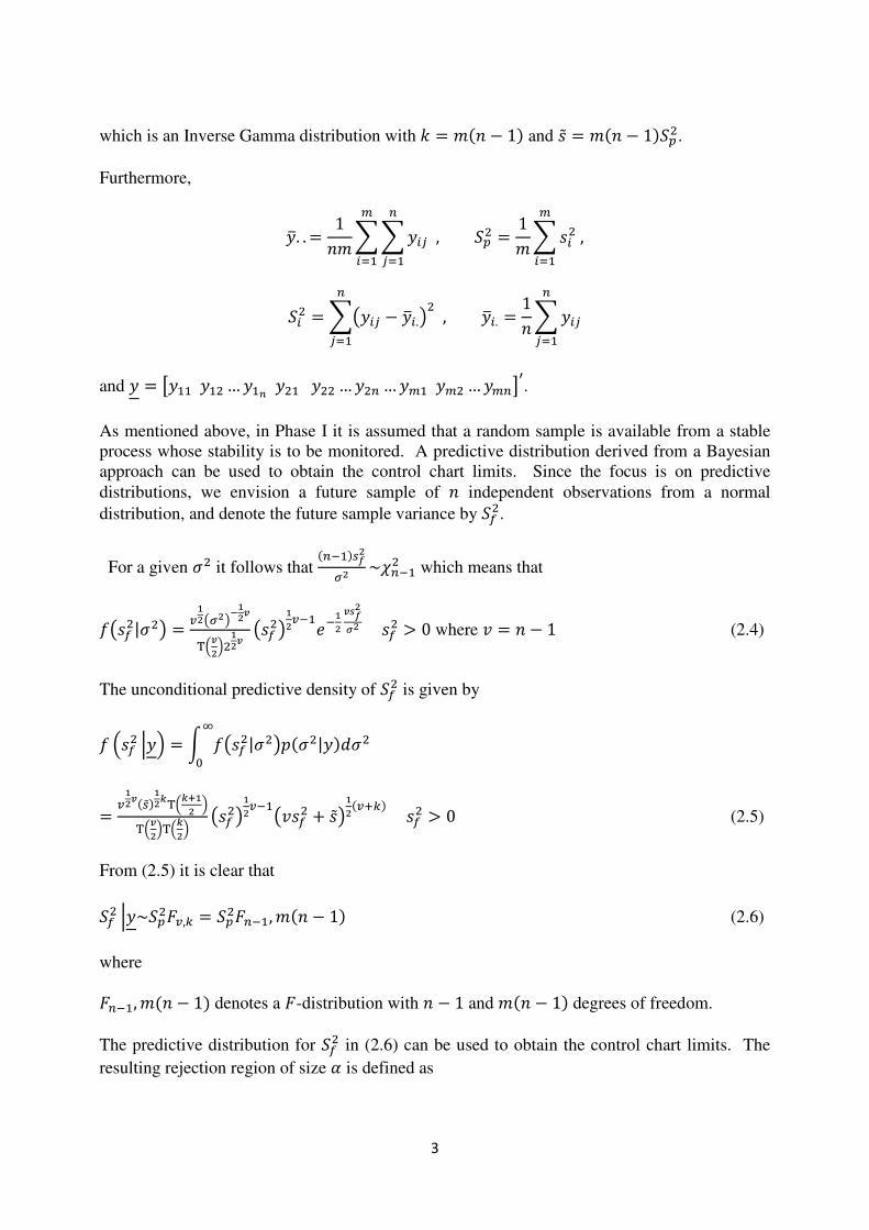
which is an Inverse Gamma distribution with 6 = − 1 and 8 = − 19:.

Furthermore,

;. . = 1 < < , 9: = 1

$

=-

%

=-< 8 ,

%

=-

9 = <> − ;.? , ;. = 1 <

$

=-

$

=-

and = @-- - … -A - … $ … %- % … %$BC.

As mentioned above, in Phase I it is assumed that a random sample is available from a stable

process whose stability is to be monitored. A predictive distribution derived from a Bayesian

approach can be used to obtain the control chart limits. Since the focus is on predictive

distributions, we envision a future sample of independent observations from a normal

distribution, and denote the future sample variance by 9D.

For a given it follows that $-)E#

"# ~F$- which means that

>8D| '? = H+#>"#?I+

#J

K J#&+

#J >8D?+#H-1+

# J2E#4# 8D > 0 where L = − 1 (2.4)

The unconditional predictive density of 9D is given by

8D '& = M >8D| '?(|'N

O

= H+#J)+

#/K /P+# &

K J#&K /

#& >8D?+#H->L8D + 8?

+#H0, 8D > 0 (2.5)

From (2.5) it is clear that

9D ~9:RH,, = 9:R$-, − 1' (2.6)

where

R$-, − 1 denotes a R-distribution with − 1 and − 1 degrees of freedom.

The predictive distribution for 9D in (2.6) can be used to obtain the control chart limits. The

resulting rejection region of size S is defined as

4

S = T 8D '& 8DUV .

Assuming that the process remains stable, this predictive distribution can also be used to derive

the distribution of the “run length”. Typically, a “future” sample of size is taken repeatedly

from the process, and one wants to determine the distribution of the “run length”, that is the

number of such samples, W, until the control chart signals for the first time. (Note that W here

does not include the sample when the control chart signals). Given and a stable process, the

distribution of the run length W is geometric with parameter X = T >8D| '?8DUV ,

where >8D| '? is given in (2.4). For given , the future samples are independent of each

other. The value of is of course unknown and the uncertainty is described by its posterior

distribution in (2.3), denoted by (|'.

The predictive distribution of the “run length” or the “average run length” can therefore easily

be simulated. The first two moments of W can also be obtained by numerical integration,

namely

YW|' = T -Z"# ( '& and YW|' = T Z>"#?

Z"# ( '& .

3. EXAMPLE

Table 3.1 displays = 20 rational subgroups, each of size = 5, simulated from a normal

distribution; for our current purpose the mean and the variance of the normal distribution from

which the samples were simulated are not mentioned because we assume that both these

parameters are unknown. Also shown in Table 3.1 are the sample variances, 9, for

= 1,2, … ,20. These data will be used to construct a Shewhart-type Phase I upper control

chart for the variance, and also to calculate the run length for a future sample of size taken

repeatedly from the process.

Table 3.1: Data for constructing Shewhart-type Phase I upper control chart for the variance

Sample number /

Time \

]\^ ]\_ ]\` ]\a ]\b c\_

1 23.0 27.8 21.5 24.3 18.9 10.93

5

2 14.2 25.9 27.3 17.9 19.1 30.77

3 24.7 16.6 22.8 26.9 21.5 15.03

4 23.6 20.8 28.4 18.6 24.5 13.95

5 14.1 20.9 18.2 19.0 28.7 28.85

6 23.0 13.4 29.4 28.4 11.6 68.83

7 19.5 14.9 23.3 12.1 11.2 26.20

8 16.8 25.5 19.2 19.7 23.6 12.39

9 15.1 18.1 22.3 18.4 23.0 10.64

10 17.5 16.0 19.1 26.8 23.1 19.42

11 26.2 24.3 22.0 21.4 25.9 4.82

12 15.9 23.2 17.8 16.6 13.8 12.41

13 14.8 17.0 19.1 13.1 15.0 5.32

14 13.8 18.3 25.0 18.2 18.5 16.03

15 28.2 23.2 16.6 18.8 18.7 21.53

16 12.9 20.0 32.2 16.4 26.1 59.47

17 22.0 11.9 21.5 21.1 17.9 17.80

18 21.1 19.4 16.3 21.8 14.3 10.23

19 16.2 21.4 25.5 14.2 28.0 34.67

20 12.5 17.2 17.9 14.4 16.5 4.92

9: = 1 < 9 = 1

20 10.93 + 30.77 + ⋯ + 4.92 = 21.21$

=-

For S = 0.01, = 5, = 20 and by using the predictive distribution defined in equation

(2.6) the upper control limit is given by 9:R$-, − 1S = 21.213.56 = 75.51.

Inspection of Table 3.1 shows that all sample variances are smaller than the upper control limit

of 75.51.

Given and a stable process the distribution of the run length W is geometric with parameter

X = T >8D| '?8DUV , where >8D| '? is defined in (2.4) and

jS = >8:R$-,%$-S ; ∞? = 75.51 ; ∞.

Therefore, for given ,

(>8D > 8:R$-,%$-S? = m "#nAI+#$- > 8: R$-,%$-S& (from (2.4))

= m o%$-)p#nqAI+# nAI+#

$- > 8: R$-,%$-Sr = m F$- > -% F%$- R$-;%$-S& (from (2.3))

= X>F%$- ? (for given F%$- (2.7)

By simulating ℓ values from a chi-square distribution with − 1 = 80 degrees of freedom

and calculating (2.7), the distribution, mean and variance of the run length W can easily be

obtained. For our example we used ℓ = 10000.

6

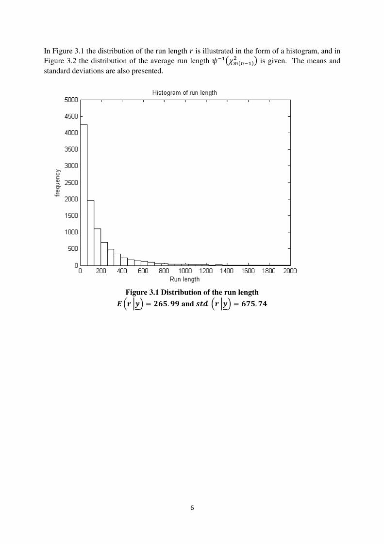
In Figure 3.1 the distribution of the run length W is illustrated in the form of a histogram, and in

Figure 3.2 the distribution of the average run length X->F%$- ? is given. The means and

standard deviations are also presented.

Figure 3.1 Distribution of the run length

u v ]'& = _wb. xx and yz v ]'& = w|b. |a

7

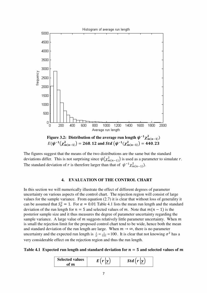
Figure 3.2: Distribution of the average run length ^~^_

Y^>~^_ ? = _w. ^_ and cz >^~^_ ? = aa. _`

The figures suggest that the means of the two distributions are the same but the standard

deviations differ. This is not surprising since X>F%$- ? is used as a parameter to simulate W.

The standard deviation of W is therefore larger than that of X-F%$- .

4. EVALUATION OF THE CONTROL CHART

In this section we will numerically illustrate the effect of different degrees of parameter

uncertainty on various aspects of the control chart. The rejection region will consist of large

values for the sample variance. From equation (2.7) it is clear that without loss of generality it

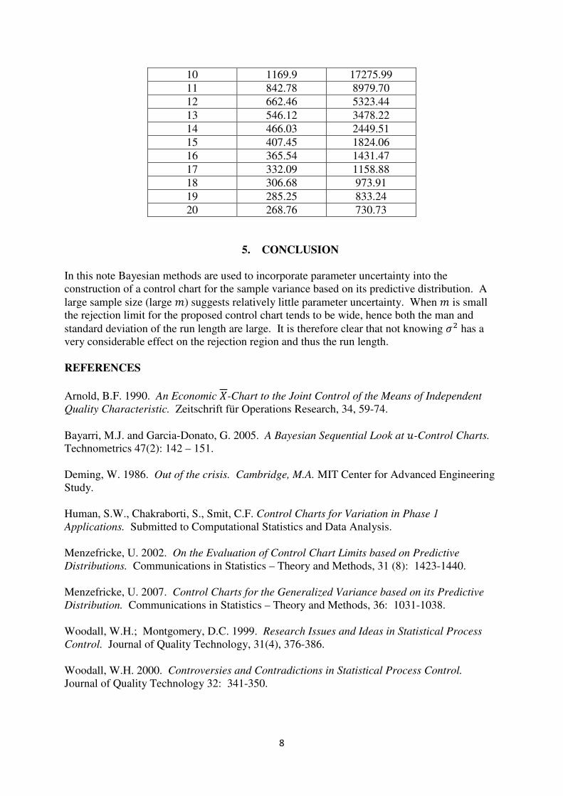
can be assumed that 9: = 1. For S = 0.01 Table 4.1 lists the mean run length and the standard

deviation of the run length for = 5 and selected values of . Note that − 1 is the

posterior sample size and it thus measures the degree of parameter uncertainty regarding the

sample variance. A large value of suggests relatively little parameter uncertainty. When

is small the rejection limit for the proposed control chart tend to be wide, hence both the mean

and standard deviation of the run length are large. When → ∞, there is no parameter

uncertainty and the expected run length is 1 10.01

100α

= = . It is clear that not knowing has a

very considerable effect on the rejection region and thus the run length.

Table 4.1 Expected run length and standard deviation for = b and selected values of

Selected values

of u v ]'& cz v ]'&

8

10 1169.9 17275.99

11 842.78 8979.70

12 662.46 5323.44

13 546.12 3478.22

14 466.03 2449.51

15 407.45 1824.06

16 365.54 1431.47

17 332.09 1158.88

18 306.68 973.91

19 285.25 833.24

20 268.76 730.73

5. CONCLUSION

In this note Bayesian methods are used to incorporate parameter uncertainty into the

construction of a control chart for the sample variance based on its predictive distribution. A

large sample size (large ) suggests relatively little parameter uncertainty. When is small

the rejection limit for the proposed control chart tends to be wide, hence both the man and

standard deviation of the run length are large. It is therefore clear that not knowing has a

very considerable effect on the rejection region and thus the run length.

REFERENCES

Arnold, B.F. 1990. An Economic -Chart to the Joint Control of the Means of Independent

Quality Characteristic. Zeitschrift für Operations Research, 34, 59-74.

Bayarri, M.J. and Garcia-Donato, G. 2005. A Bayesian Sequential Look at -Control Charts.

Technometrics 47(2): 142 – 151.

Deming, W. 1986. Out of the crisis. Cambridge, M.A. MIT Center for Advanced Engineering

Study.

Human, S.W., Chakraborti, S., Smit, C.F. Control Charts for Variation in Phase 1

Applications. Submitted to Computational Statistics and Data Analysis.

Menzefricke, U. 2002. On the Evaluation of Control Chart Limits based on Predictive

Distributions. Communications in Statistics – Theory and Methods, 31 (8): 1423-1440.

Menzefricke, U. 2007. Control Charts for the Generalized Variance based on its Predictive

Distribution. Communications in Statistics – Theory and Methods, 36: 1031-1038.

Woodall, W.H.; Montgomery, D.C. 1999. Research Issues and Ideas in Statistical Process

Control. Journal of Quality Technology, 31(4), 376-386.

Woodall, W.H. 2000. Controversies and Contradictions in Statistical Process Control.

Journal of Quality Technology 32: 341-350.

9

Woodward, P.W.; Naylor, J.C. 1993. An Application of Bayesian Methods in SPC. The

Statistician, 42, 461-469.

ON TERMINATING POISSON PROCESSES

IN SOME SHOCK MODELS

Maxim Finkelstein

Department of Mathematical Statistics

University of the Free State, Bloemfontein,

and

Francois Marais

CSC, Cape Town, South Africa

ABSTRACT. A system subject to a point process of shocks is considered. Shocks

occur in accordance with the homogeneous Poisson process. Different criteria of sys-

tem failure (termination) are discussed and the corresponding probabilities of failure

(accident) free performance are derived. The described analytical approach is based

on deriving integral equations for each setting and solving these equations via the

Laplace transform. Some approximations are analyzed and further generalizations and

applications are discussed.

Keywords: Poisson process, shocks, probability of termination, Laplace transform,

time of recovery

1. INTRODUCTION

Consider first, a general point process ,...2,1,0,,0; 10 =>= + nTTTT nnn , where nT

is time to the n th arrival of an event with the corresponding cumulative distribution

function (Cdf) )()( tF n . Let G be a geometric variable with parameter θ (indepen-

dent of 0 ≥nnT ) and denote by T a random variable with the following Cdf:

∑∞

=

−=1

)(1 )(),(k

kktFtF θθθ , (1)

where θθ −= 1 .

A natural reliability interpretation of model (1) is via the stochastic point process

of shocks. Let T be a random time to failure (termination) of a system subject to a

point process of shocks [1]. We interpret the term “shock” in a very broad sense as

some instantaneous, potentially harmful event. Assume for simplicity that a shock is

the only cause of failure. It means that a system is ‘absolutely reliable’ in the absence

of shocks. Assume also that each shock independently of the previous history leads to

a system failure with probability θ and is survived with probability θθ −= 1 . This

procedure defines the terminating point process, whereas the corresponding survival

probability of our system (reliability) in ),0( t is ),(1),( θθ tFtP −≡ .

Obtaining probability ),( θtP is an important problem in various reliability and

safety assessment applications. As described, the shock can have an interpretation of a

‘killing’ event. Alternatively, a shock process can have a meaning of a process of de-

mands for service, whereas the survival probability is the probability that all demands

are serviced. Another interpretation is when a repairable system described by the al-

ternating renewal process should be just available at each instance of demand. In this

2

case the survival probability has a meaning of multiple availability [2], which is a ge-

neralization of the conventional availability.

It is clear that a general relationship (1) does not allow for explicit results that can

be used in practice and therefore, assumptions on the form of the point process should

be made. Two specific point processes are mostly used in reliability applications, i.e.,

the Poisson process and the renewal process. This paper is devoted to the case of the

Poisson process of shocks. Some results for the terminating renewal processes can be

found, e.g., in reference [3]. Also see the discussion in Section 5.

Consider the Poisson process of shocks with rate λ . In this case the survival prob-

ability can be easily explicitly obtained [4]:

( )∑

∞

−==≥0 !

exp)(),(]Pr[k

tttPtT

k

k λλθθ

exp tλθ−= . (2)

It follows from equation (2) that the corresponding failure rate, which describes the

lifetime of our system T , is given by a simple and meaningful relationship:

λθλ =)(t . (3)

Thus, the rate of the underlying Poisson process λ is decreased by the factor 1≤θ .

Equation (3) describes an operation of thinning of the Poisson process for this specific

case [5].

The main methodological aim of this paper is to show how the method of integral

equations can be effectively applied to obtaining probability ),( θtP in various set-

tings. In order to illustrate this claim in the simplest way, let us derive (2) using the

corresponding integral equation and the subsequent Laplace transform. It is easy to

see that the following equation with respect to ),( θtP holds:

dxxtPeetP

t

xt ),(),(0

θθλθ λλ −+= ∫−− . (4)

Indeed, the first term on the right hand side is the probability that there are no shocks

in ),0[ t and the integrand defines the probability that the first shock has occurred in

),[ dxxx + , was survived and then the system has survived in ),[ tx . Due to the prop-

erties of the homogeneous Poisson process, the probability of the latter event is

),( θxtP − .

Applying the Laplace transform to both sides of equation (4) results in

λθθθ

λ

θλ

λθ

+=⇒

++

+=

ssPsP

sssP

1),(

~),(

~1),(

~, (5)

where ),(~

θsP denotes the Laplace transform of ),( θtP . The corresponding inversion,

as in (2), results in exp tλθ− .

Note that this solution is due to the fact that the Laplace transform can be nicely

obtained for the case of the (homogeneous) Poisson process. For the nonhomogeneous

Poisson process (NHPP) with rate )(tλ , similar to (2), direct summation gives

3

∑ ∫∫

∫∞

−=

−=0 0

0

0

)(exp!

)(

)(exp)(),(

t

kt

t

k duuk

duu

duutP λθ

λ

λθθ .

Generalization of integral equation (4) to the case of NHHP is not so straightforward

but in principle can be performed (see Section 5). However, it is difficult to apply the

‘explicit’ Laplace transform in this case. Therefore, our models will be considered

only for homogeneous Poisson processes of shocks.

We will discuss three models for obtaining survival probability in different set-

tings. Other settings and generalizations can be studied as well. The main analytical

tool allowing for explicit solutions in all considered situations is the method of

integral equations and the subsequent application of the Laplace transform. Section 2

is devoted to the case when probability of termination depends on the quality of the

repairable system’s performance at the time of a shock arrival. This is a natural as-

sumption, as resistance to a shock often depends on the state of a system. Section 3

deals with additional source of termination of the process when the shocks are too

close and a system has not enough time to recover after the previous shock. In Section

4, two different types of shocks are considered. Two consecutive shocks of the first

kind can kill a system, but if there is a shock of another kind between them, the sys-

tem survives.

2. POBABILITY OF TERMINATION DEPENDS ON A SYSTEM’S STATE

Consider a repairable system with instantaneous, perfect repair that starts functioning

at 0=t . Let its lifetime be described by the Cdf )(tF , which is a governing distribu-

tion for the corresponding renewal process with the renewal density function to be

denoted by )(th . Assume that the quality of performance of our system is character-

ized by some deterministic for simplicity function of performance )(tQ to be called

the quality function [6]. The considered approach can be generalized to the case of a

random )(tQ . It is often a decreasing function of time, and this assumption is quite

natural for degrading systems. In applications, the function )(tQ can describe some

key parameter of a system, e.g., the decreasing in time accuracy of the information

measuring system or effectiveness (productivity) of some production process. As re-

pair is perfect, the quality function is also restored to its initial value )0(Q . It is clear

that the quality function of our system at time t is now random and equal to )(YQ ,

where Y is a random time since the last (before t ) repair.

The system is subject to the Poisson process of shocks with rate λ . As previously,

each shock can terminate the performance of the repairable system and we are inter-

ested in obtaining the survival probability ),( θtP . Note that the repaired failure of the

system does not terminate the process and only a shock can result in termination. As-

sume that the probability of termination depends on the system’s quality at the time of

a shock, which is a reasonable assumption, i.e., the larger the value of quality, the

smaller the probability of termination. Let the first shock arrive before the first failure

of the system. Denote by ))((* tQθ the corresponding probability of termination in

this case. Now we are able to obtain )(tθ -the probability of termination of the operat-

ing system by the first shock at time instant t (and not necessarily before the first fail-

4

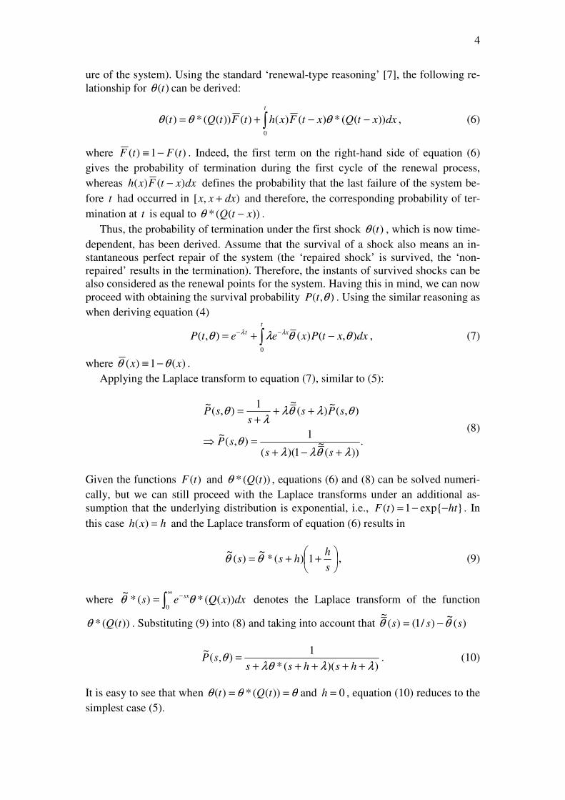
ure of the system). Using the standard ‘renewal-type reasoning’ [7], the following re-

lationship for )(tθ can be derived:

∫ −−+=t

dxxtQxtFxhtFtQt0

))((*)()()())((*)( θθθ , (6)

where )(1)( tFtF −≡ . Indeed, the first term on the right-hand side of equation (6)

gives the probability of termination during the first cycle of the renewal process,

whereas dxxtFxh )()( − defines the probability that the last failure of the system be-

fore t had occurred in ),[ dxxx + and therefore, the corresponding probability of ter-

mination at t is equal to ))((* xtQ −θ .

Thus, the probability of termination under the first shock )(tθ , which is now time-

dependent, has been derived. Assume that the survival of a shock also means an in-

stantaneous perfect repair of the system (the ‘repaired shock’ is survived, the ‘non-

repaired’ results in the termination). Therefore, the instants of survived shocks can be

also considered as the renewal points for the system. Having this in mind, we can now

proceed with obtaining the survival probability ),( θtP . Using the similar reasoning as

when deriving equation (4)

dxxtPxeetP

t

xt ),()(),(0

θθλθ λλ −+= ∫−− , (7)

where )(1)( xx θθ −≡ .

Applying the Laplace transform to equation (7), similar to (5):

.))(

~1)((

1),(

~

),(~

)(~1

),(~

λθλλθ

θλθλλ

θ

+−+=⇒

+++

=

sssP

sPss

sP

(8)

Given the functions )(tF and ))((* tQθ , equations (6) and (8) can be solved numeri-

cally, but we can still proceed with the Laplace transforms under an additional as-

sumption that the underlying distribution is exponential, i.e., exp1)( httF −−= . In

this case hxh =)( and the Laplace transform of equation (6) results in

++=

s

hhss 1)(*

~)(

~θθ , (9)

where dxxQessx ))((*)(*

~

0θθ ∫

∞−= denotes the Laplace transform of the function

))((* tQθ . Substituting (9) into (8) and taking into account that )(~

)/1()(~

sss θθ −=

))((*

1),(

~

λλλθθ

+++++=

hshsssP . (10)

It is easy to see that when θθθ == ))((*)( tQt and 0=h , equation (10) reduces to the

simplest case (5).

5

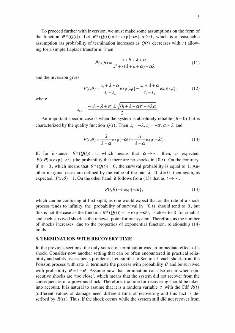
To proceed further with inversion, we must make some assumptions on the form of

the function ))((* tQθ . Let 0,exp1))((* ≥−−= ααθ ttQ , which is a reasonable

assumption (as probability of termination increases as )(tQ decreases with t ) allow-

ing for a simple Laplace transform. Then

αλαλ

αλθ

++++

+++=

)(),(

~2 hss

hssP (11)

and the inversion gives

expexp),( 2

21

21

21

1 tsss

sts

ss

stP

−

++−

−

++=

αλαλθ , (12)

where

2

4)()( 2

2,1

λααλαλ −++±++−=

hhs .

An important specific case is when the system is absolutely reliable ( )0=h but is

characterized by the quality function )(tQ . Then λααλ ≠−=−= ;, 21 ss and

expexp),( tttP λαλ

αα

αλ

λθ −

−−−

−= . (13)

If, for instance, 1))((* =tQθ , which means that ∞→α , then, as expected,

exp),( ttP λθ −= (the probability that there are no shocks in ),0[ t . On the contrary,

if 0=α , which means that 0))((* =tQθ , the survival probability is equal to 1. An-

other marginal cases are defined by the value of the rate λ . If 0=λ , then again, as

expected, 1),( =θtP . On the other hand, it follows from (13) that as ∞→t ,

exp),( ttP αθ −→ , (14)

which can be confusing at first sight, as one would expect that as the rate of a shock

process tends to infinity, the probability of survival in ),0[ t should tend to 0 , but

this is not the case as the function ,exp1))((* ttQ αθ −−= is close to 0 for small t

and each survived shock is the renewal point for our system. Therefore, as the number

of shocks increases, due to the properties of exponential function, relationship (14)

holds.

3. TERMINATION WITH RECOVERY TIME

In the previous sections, the only source of termination was an immediate effect of a

shock. Consider now another setting that can be often encountered in practical relia-

bility and safety assessments problems. Let, similar to Section 1, each shock from the

Poisson process with rate λ terminate the process with probability θ and be survived

with probability θθ −= 1 . Assume now that termination can also occur when con-

secutive shocks are ‘too close’, which means that the system did not recover from the

consequences of a previous shock. Therefore, the time for recovering should be taken

into account. It is natural to assume that it is a random variable τ with the Cdf )(tR

(different values of damage need different time of recovering and this fact is de-

scribed by )(tR ). Thus, if the shock occurs while the system still did not recover from

6

the previous one, it terminates the process. It is the simplest criterion of termination of

this kind. Other criterions can be also considered. As previously, we want to derive

),,( RtP θ -the probability of survival in ),0[ t .

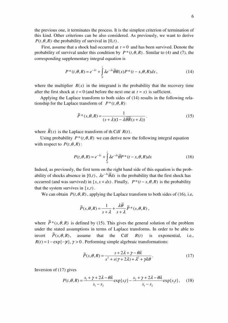
First, assume that a shock had occurred at 0=t and has been survived. Denote the

probability of survival under this condition by ),,(* RtP θ . Similar to (4) and (7), the

corresponding supplementary integral equation is

dxRxtPxReeRtP

t

xt ),,(*)(),,(*0

θθλθ λλ −+= ∫−− , (14)

where the multiplier )(xR in the integrand is the probability that the recovery time

after the first shock at 0=t (and before the next one at )xt = is sufficient.

Applying the Laplace transform to both sides of (14) results in the following rela-

tionship for the Laplace transform of ),,(* RtP θ :

))(~

1)((

1),,(*

~

λθλλθ

+−+=

sRsRsP , (15)

where )(~

sR is the Laplace transform of th Cdf )(tR .

Using probability ),,(* RtP θ we can derive now the following integral equation

with respect to ),,( RtP θ :

dxRxtPeeRtP

t

xt ),,(*),,(0

θθλθ λλ −+= ∫−−

(16)

Indeed, as previously, the first term on the right hand side of this equation is the prob-

ability of shocks absence in ),0[ t , dxexθλ λ− is the probability that the first shock has

occurred (and was survived) in ),[ dxxx + . Finally, ),,(* RxtP θ− is the probability

that the system survives in ),[ tx .

We can obtain ),,( RtP θ , applying the Laplace transform to both sides of (16), i.e,

),,(*~1

),,(~

RsPss

RsP θλ

θλ

λθ

++

+= ,

where ),,(*~

RsP θ is defined by (15). This gives the general solution of the problem

under the stated assumptions in terms of Laplace transforms. In order to be able to

invert ),,(~

RsP θ , assume that the Cdf )(tR is exponential, i.e.,

0,exp1)( >−−= γγttR . Performing simple algebraic transformations:

γλθλλγ

θλγλθ

++++

−++=

22 )2(

2),,(

~

ss

sRsP . (17)

Inversion of (17) gives

exp2

exp2

),,( 2

21

21

21

1 tsss

sts

ss

sRtP

−

−++−

−

−++=

θλλγθλλγθ , (18)

7

where

2

)(4)2()2( 22

2,1

γλθλλγλγ +−+±+−=s .

Equation (18) gives an exact solution for ),,( RtP θ . In applications it is convenient

to use simple approximate formulas. Consider the following assumption:

∫∞

−≡>>0

))(1(1

dxxRτλ

, (19)

where τ denotes the mean time of recovery.

Relationship (19) means that the mean inter-arrival time in the shock process is

much larger than the mean time of recovery, and this is often the case in practice. In

the study of repairable systems, the similar case is usually called the fast repair condi-

tion. Using this assumption, similar to (3), the equivalent rate of termination for our

process for 0→τλ , 1>>tλ can be written as

))1(1()( oBt += λλ , (20)

where B is the probability of termination for the occurred shock due to two causes,

i.e., the termination immediately after the shock and the termination when the next

shock occurs before the recovery is completed. Therefore, for sufficiently large t

( τ>>t ) the integration in the following integral can be performed to ∞ and the ap-

proximate value of B is

∫∞

− −−+=0

))(1()1( dxxReBxλλθθ ,

Assuming, as previously, 0,exp1)( >−−= γγttR gives

γλ

θγλ

+

+=B .

Finally, the fast repair approximation for the survival probability is

+

+−≈ tRtP

γλ

θγλθ exp),,( . (21)

It can be easily seen that when ∞→γ (instant recovery), relationship (21) reduces to

equation (2). Note that approximate relation (20) is derived for all shocks except the

first one (for which θ=B ), but the condition 1>>tλ (large expected number of

shocks in ),0[ t ) ensures that the error in (21) due to this cause is sufficiently small.

The accuracy of the fast repair approximation (21) with respect to the time of recov-

ery can be analyzed similar to reference [2].

4. TWO TYPES OF SHOCKS

Assume now that there are two types of shocks. As in the previous section, potentially

harmful shocks (to be called red shocks) result in termination of the process when

they are ‘too close’, i.e., when the time between two consecutive red shocks is smaller

8

then a recovery time with the Cdf )(tR . Therefore, in this case a system does not have

enough time to recover from the consequences of the previous red shock. Assume for

simplicity that the probability of immediate termination on red shock’s occurrence is

equal to 0 ( 0=θ ). The model can be easily generalized to this case as well. On the

other hand, our system is subject to the process of ‘good’ (blue) shocks. If the blue

shock follows the red shock, termination cannot happen no matter how soon the next

red shock will occur. Therefore, the blue shock can be considered as a kind of addi-

tional recovery action.

Denote by λ and β the rates of the independent Poisson processes of red and blue

shocks respectively. First, assume that the first red shock has already occurred at

0=t . An integral equation for the probability of survival in ),0[ t , ),,(* RtP β for

this case is as follows:

dydxRyxtPeeeeRtP

t xt

yxxt ),,(*),,(*0 0

βλββ λλβλ −−+= ∫ ∫−

−−−−

dxRxtPxRee

t

xx ),,(*)(0

βλ λβ −+ ∫−− , (22)

where

• The first term on the right hand side is the probability that there are no other red

shocks in ),0[ t ;

• dxee xx λββ −− is the probability that a blue shock occurs in ),[ dxxx + and no red

shocks occur in ),0( x ;

• dye yλλ − is the probability that the second red shock occurs in ),[ dyyxyx +++ ;

• ),,(* RyxtP β−− is the probability that the system survives in ),[ tyx + given

the red shock has occurred at time yx + ;

• dxeexx λβ λ −− is the probability that there is one red shock (the second) in ),0( t and

no blue shocks in this interval of time;

• )(xR is the probability that the recovery time x is sufficient and therefore the

second red shock does not terminate the process;

• ),,(* RxtP β− is the probability that the system survives in ),[ tx given the red

shock has occurred at time x .

Using ),,(* RtP β that can be obtained from equation (22) we can now construct an

integral equation with respect to ),,( RtP β -the probability of survival without assum-

ing occurrence of the red shock at 0=t . Similar to (16)

dxRxtPeeRtP

t

xt ),,(*),,(0

βλβ λλ −+= ∫−− . (23)

Applying the Laplace transform to equation (22) results in

)(~

))(())((),,(*

~

λβλλβλβλλλβ

λββ

+++++−−+++

++=

sRssss

sRsP . (24)

Applying the Laplace transform to equation (23):

9

),,(*~1

),,(~

RsPss

RsP βλ

λ

λβ

++

+= . (25)

This equation gives a general solution of the problem under the stated assumptions in

terms of Laplace transforms. In order to be able to invert ),,(~

RsP β , as in the pre-

vious section, assume that the Cdf )(tR is exponential: 0,exp1)( >−−= γγttR .

Performing simple algebraic transformations

22 )2(

2),,(

~

λλβγ

λβγβ

++++

+++=

ss

sRsP . (26)

Inversion of (26) gives

exp2

exp2

),,( 2

21

21

21

1 tsss

sts

ss

sRtP

−

+++−

−

+++=

λβγλβγβ , (27)

where

2

)(4)()2( 2

2,1

βγλβγβλγ +++±++−=s .

When γ =0, there is no recovery time and the process is terminated when two consec-

utive red shocks occur. In this case equation (27) reduces to relationship obtained in

reference [8].

Equation (27) gives an exact solution for ),,( RtP θ . Similar to Section 3, it can be

simplified under certain assumptions. Assume that the fast repair condition (19) holds.

The first red shock cannot terminate the process. The probability that the subsequent

shock can result in termination is

∫ ∫−

−−− −=t xt

yyxdydxyReeeB

0 0

))(1(βλλ λλ . (28)

For the exponentially distributed time of recovery:

tteeB

)(2

))((

γβλλ

γβγβλ

λ

γβ

λ

γβλ

λ ++−−

++++

+−

++=

For sufficiently large t , λβλλ ++≈ /B and this approximate value can be used for

subsequent shocks as well. Therefore, relationship

++−≈ tRtP

γβλ

λθ

2

exp),,( .

is the fast repair approximation in this case.

5. DISCUSSION

The method of integral equations, which is applied to deriving the survival probability

for different shock models is an effective tool for obtaining probabilities of interest in

10

situations where the object under consideration has renewal points. As the considered

process of shocks is the homogeneous Poisson process, each shock (under some addi-

tional assumptions) constitutes these renewal points. When a shock process is NHPP,

there are no renewal points, but the integral equations can be usually also derived. For

illustration, consider the corresponding generalization of equation (4). Denote by

),,( θxxtP − the survival probability in txtx <),,[ for the ‘remaining shock process’

that started at 0=t and was not terminated by the first shock at time x . Note that this

probability depends now not only on tx − as in the homogeneous case but on x as

well. Equation (4) is modified now to

dxxtPduuxduutP

t xt

),()(exp)()(exp),(0 00

θθλλλθ −

−+

−= ∫ ∫∫

It can be easily seen by substitution that

txduuxxtP

t

x

,0,)(exp),,( ≤

−=− ∫λθθ

is the solution of this equation.

One can formally write integral equations for other models considered in this paper

and the NHPP process of shocks, but their solutions should be obtained numerically

as the explicit inversions of the corresponding Laplace transforms are not possible.

If shocks are described by the renewal process with the governing distribution

)(tF and the corresponding probability density function )(tf , the method of integral

equations can be also obviously applied as in this case we also have ‘pure renewal

points’. For instance, the simplest equation (4) turns in this case into

dxxtPxftFtP

t

),()()(1(),(0

θθθ −+−= ∫ .

Applying the Laplace transform gives

))(~

1(

)(~

1),(

~

sfs

sfsP

θθ

−

−= ,

which is formally a solution to our problem in terms of the Laplace transform. Note

that for given )(tF it can be inverted usually only numerically. This is similar to the

reasoning used for describing the Laplace transforms for standard renewal equations

in the renewal theory [9].

Another generalization of (4) (and subsequent models) is to the case when )(tθ is

a time-dependent probability. It is well-known that the probability of survival for the

NHPP of shocks in this case is given by the following relationship:

−= ∫t

duuuttP0

)()(exp))(,( λθθ ,

which is an analogue of the Brown-Proschan model in the theory of imperfect (mi-

nimal) repair [10].

References

11

1. Barlow R. and Proschan F. (1975). Statistical Theory of Reliability and Life Test-

ing Probability Models, Holt, Rinehart and Winston. 1975.

2. Finkelstein M.S. and Zarudnij V.I. (2202) Laplace transform methods and fast re-

pair approximations for multiple availability and its generalizations, IEEE Trans-

actions on Reliability, 51, 168-177.

3. Finkelstein M.S. (2003). Simple bounds for terminating Poisson and renewal

processes, Journal of Statistical Planning and Inference, 113, 541-548.

4. Thompson W.A. (1988). Point Process Models with Applications to Safety and

Reliability, Chapman and Hall.

5. Cox D.R. and Isham V. (1984). Point Processes, Chapman and Hall, London.

6. Finkelstein M.S. (2008). Failure Rate Modeling for Reliability and Risk, Springer.

7. Ross S.M. (1996). Stochastic Processes. John Wiley.

8. Venter J.P. (2007)………….. University of the Free State, M.Sc thesis.

9. Beichelt F.E. and Fatti L.P. (2002). Stochastic Processes and their Applications,

Taylor and Francis.

10. Block H.W, Borges W, Savits T.H. (1985). Age dependent minimal repair, Jour-

nal of Applied Probability, 22, 370-386.

1

Investigating approximations and parameter estimation of the Multivariate Generalized

Burr-Gamma

A Verster and DJ de Waal

Department Mathematical Statistics and Actuarial Science

University of the Free State

Bloemfontein

ABSTRACT

The MGBG is considered for modelling multivariate data especially containing extreme values.

This article is an extension and comparison to an earlier article by Beirlant et al. (2000).

Special attention is given to the approximations of the expected value and covariance of the

MGBG and to the estimation of parameters. The Kolmogorov-Smirnov is considered for

estimating some of the parameters.

KEYWORDS: MGBG, Extreme Values, Estimation, Approximation, Kolmogorov-

Smirnov, QQ-plot.

1. INTRODUCTION

The multivariate Generalized Burr-Gamma (MGBG) distribution (Beirlant et al., 2000)

generalizes the Burr-Gamma distribution (Beirlant et al., 2002) to a multivariate distribution

which is fairly flexible to fit to multivariate data containing extremes on all or some of the

variables. In this paper an alternative approach to Beirlant et al. (2000) is taken to estimate the

parameters of the MGBG. In Section 2 properties of the MGBG are given and in Section 3

asymptotic formulae are derived for and . These results are tested for a few

simulated data sets in Section 4. In Section 5 we discuss our alternative approach to estimate

the parameters and then the procedure is applied to a simulated data set in Section 6. Section 7

shows the difference in the estimated parameter values between the approach in Beirlant et al.

(2000) and our approach.

2. THE MULTIVARIATE GENERALIZED BURR-GAMMA DISTRIBUTION

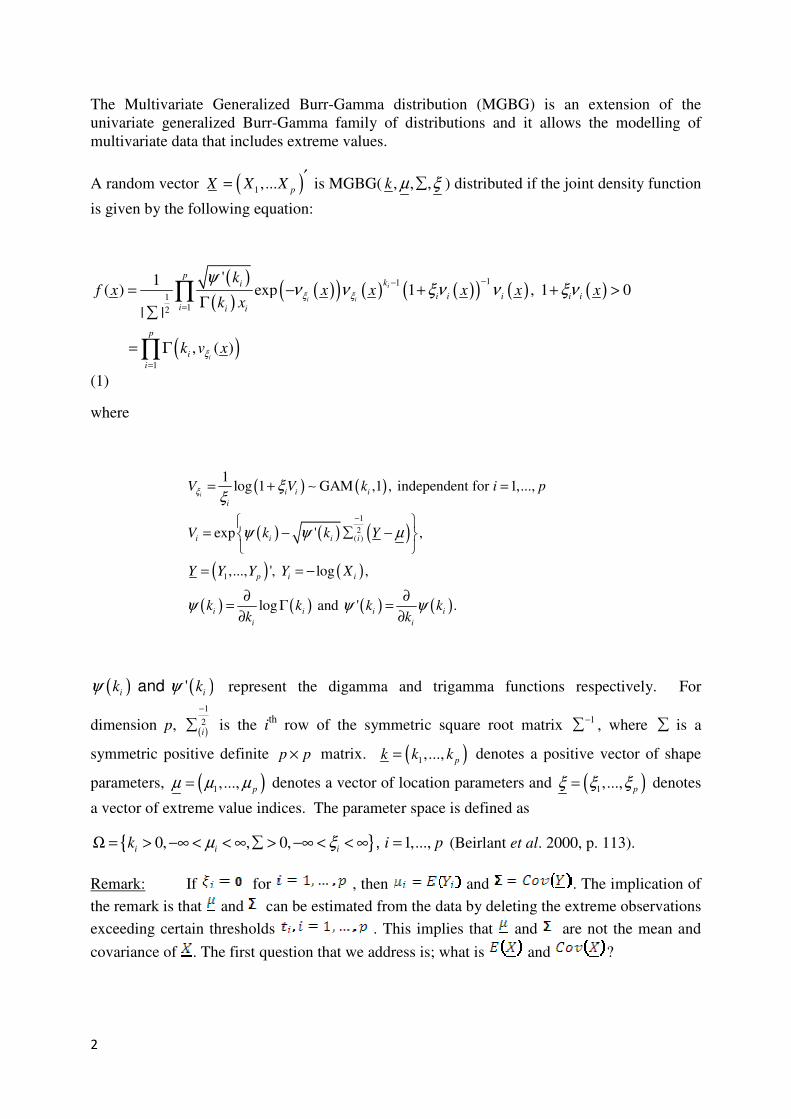
2

The Multivariate Generalized Burr-Gamma distribution (MGBG) is an extension of the

univariate generalized Burr-Gamma family of distributions and it allows the modelling of

multivariate data that includes extreme values.

A random vector ( )1 ,...p

X X X′= is MGBG( , , ,k µ ξ∑ ) distributed if the joint density function

is given by the following equation:

( )( )

( )( ) ( ) ( )( ) ( ) ( )

( )

11

112

1

'1( ) exp 1 , 1 0

| |

, ( )

i

i i

i

pki

i i i i i

i i i

p

i

i

kf x x x x x x

k x

k v x

ξ ξ

ξ

ψν ν ξν ν ξν

−−

=

=

= − + + >Γ

∑

= Γ

∏

∏

(1)

where

( ) ( )

( ) ( ) ( )

( ) ( )

( ) ( ) ( ) ( )

1

2( )

1

1log 1 GAM ,1 , independent for 1,...,

exp ' ,

,..., ', log ,

log and ' .

i i i i

i

i i i i

p i i

i i i i

i i

V V k i p

V k k Y

Y Y Y Y X

k k k kk k

ξ ξξ

ψ ψ µ

ψ ψ ψ

−

= + =

= − ∑ −

= = −

∂ ∂= Γ =

∂ ∂

∼

( ) ( )' and i ik kψ ψ represent the digamma and trigamma functions respectively. For

dimension p, ( )

1

2i

−

∑ is the ith

row of the symmetric square root matrix 1−∑ , where ∑ is a

symmetric positive definite p p× matrix. ( )1,...,

pk k k= denotes a positive vector of shape

parameters, ( )1,...,

pµ µ µ= denotes a vector of location parameters and ( )1

,...,p

ξ ξ ξ= denotes

a vector of extreme value indices. The parameter space is defined as

0, , 0, 1,...,i i ik i pµ ξΩ = > −∞ < < ∞ ∑ > −∞ < < ∞ =, (Beirlant et al. 2000, p. 113).

Remark: If for , then and . The implication of

the remark is that and can be estimated from the data by deleting the extreme observations

exceeding certain thresholds . This implies that and are not the mean and

covariance of . The first question that we address is; what is and ?

3

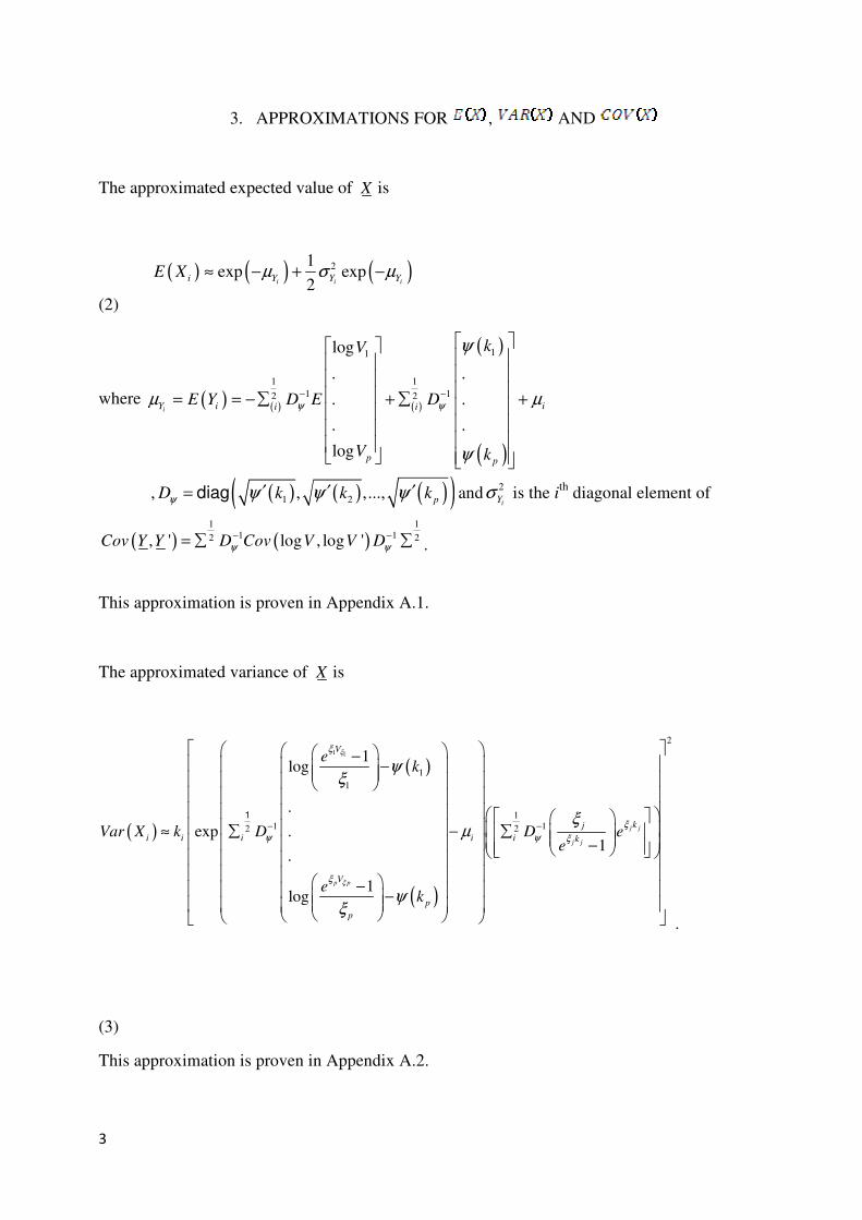
3. APPROXIMATIONS FOR , AND

The approximated expected value of X is

( ) ( ) ( )21exp exp

2i i ii Y Y YE X µ σ µ≈ − + −

(2)

where ( ) ( ) ( )

( )

( )

11

1 1

1 12 2

log

. .

. .

. .

log

iY i ii i

p p

kV

E Y D E D

V k

ψ ψ

ψ

µ µ

ψ

− −

= = −∑ + ∑ +

, ( ) ( ) ( )( )1 2, ,...,p

D k k kψ ψ ψ ψ′ ′ ′= diag and2

iYσ is the ith

diagonal element of

( ) ( )1 1

1 12 2, ' log , log 'Cov Y Y D Cov V V Dψ ψ− −= ∑ ∑ .

This approximation is proven in Appendix A.1.

The approximated variance of X is

( )

( )

( )

1 1

2

1

1

1

1 12 2

1log

.

exp .1

.

1log

j j

j j

p p

V

kj

i i i i i k

V

p

p

ek

Var X k D D ee

ek

ξ

ξ

ξ

ξ

ψ ψ ξ

ξ

ψξ

ξµ

ψξ

− −

− − ≈ ∑ − ∑ − − −

1

.

(3)

This approximation is proven in Appendix A.2.

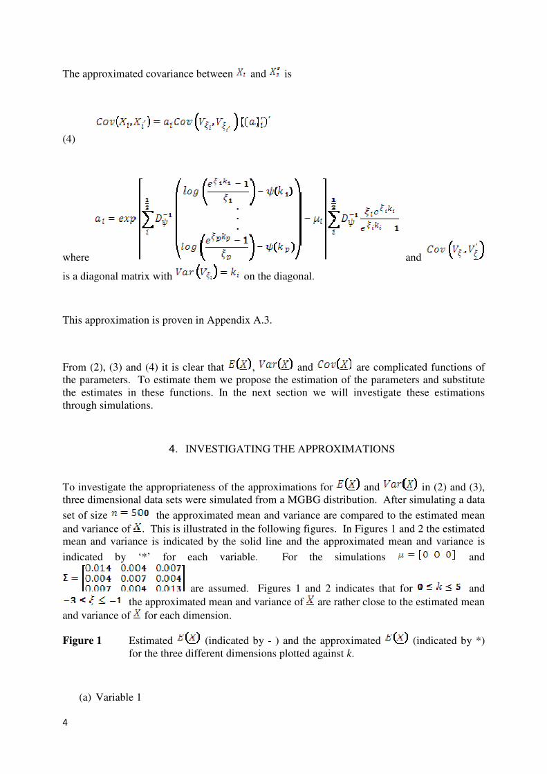
4

The approximated covariance between and is

(4)

where and

is a diagonal matrix with on the diagonal.

This approximation is proven in Appendix A.3.

From (2), (3) and (4) it is clear that , and are complicated functions of

the parameters. To estimate them we propose the estimation of the parameters and substitute

the estimates in these functions. In the next section we will investigate these estimations

through simulations.

4. INVESTIGATING THE APPROXIMATIONS

To investigate the appropriateness of the approximations for and in (2) and (3),

three dimensional data sets were simulated from a MGBG distribution. After simulating a data

set of size the approximated mean and variance are compared to the estimated mean

and variance of . This is illustrated in the following figures. In Figures 1 and 2 the estimated

mean and variance is indicated by the solid line and the approximated mean and variance is

indicated by ‘*’ for each variable. For the simulations and

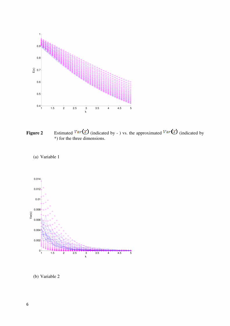
are assumed. Figures 1 and 2 indicates that for and

the approximated mean and variance of are rather close to the estimated mean

and variance of for each dimension.

Figure 1 Estimated (indicated by - ) and the approximated (indicated by *)

for the three different dimensions plotted against k.

(a) Variable 1

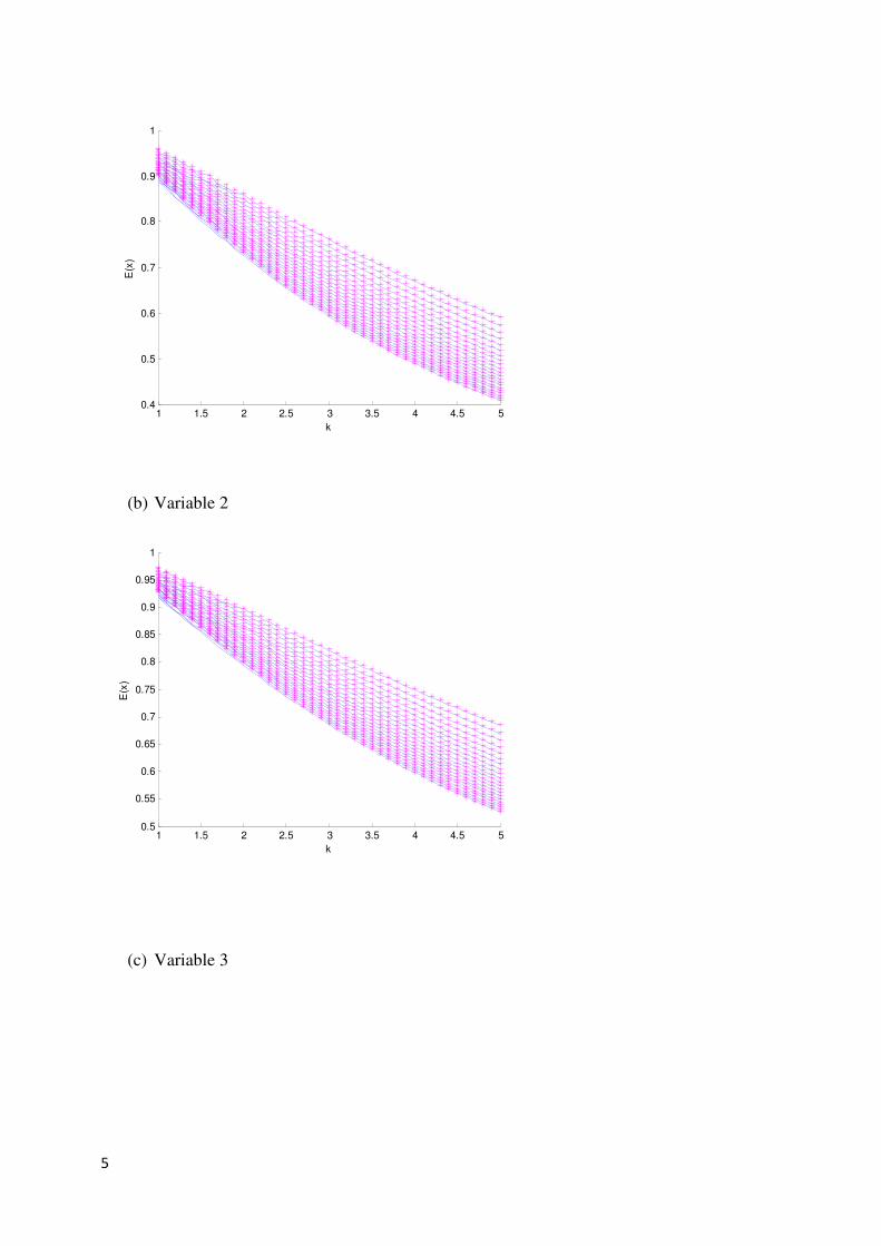
5

1 1.5 2 2.5 3 3.5 4 4.5 50.4

0.5

0.6

0.7

0.8

0.9

1

k

E(x

)

(b) Variable 2

1 1.5 2 2.5 3 3.5 4 4.5 50.5

0.55

0.6

0.65

0.7

0.75

0.8

0.85

0.9

0.95

1

k

E(x

)

(c) Variable 3

6

1 1.5 2 2.5 3 3.5 4 4.5 50.4

0.5

0.6

0.7

0.8

0.9

1

k

E(x

)

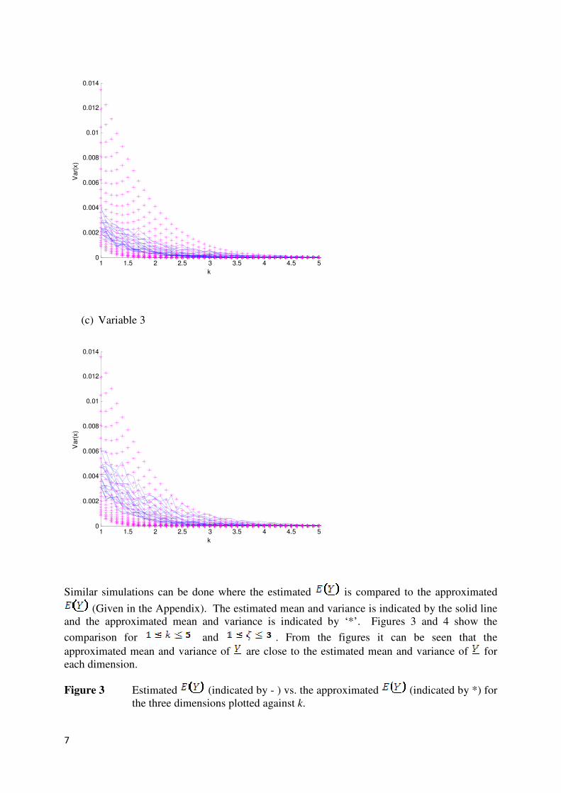
Figure 2 Estimated (indicated by - ) vs. the approximated (indicated by

*) for the three dimensions.

(a) Variable 1

1 1.5 2 2.5 3 3.5 4 4.5 50

0.002

0.004

0.006

0.008

0.01

0.012

0.014

k

Var(

x)

(b) Variable 2

7

1 1.5 2 2.5 3 3.5 4 4.5 50

0.002

0.004

0.006

0.008

0.01

0.012

0.014

k

Var(

x)

(c) Variable 3

1 1.5 2 2.5 3 3.5 4 4.5 50

0.002

0.004

0.006

0.008

0.01

0.012

0.014

k

Var(

x)

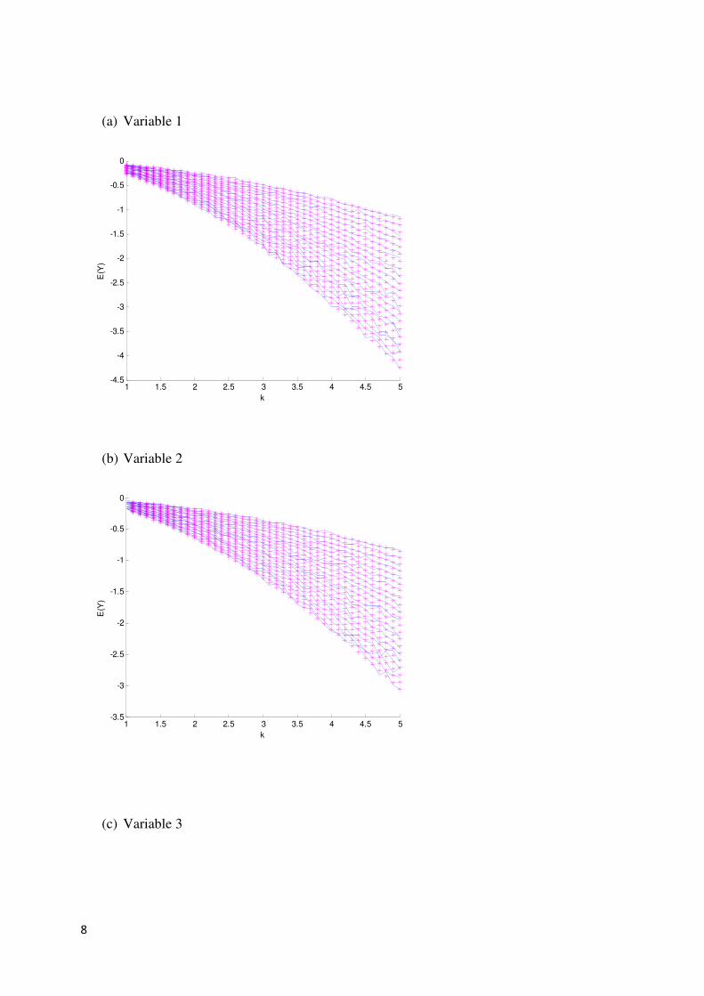
Similar simulations can be done where the estimated is compared to the approximated

(Given in the Appendix). The estimated mean and variance is indicated by the solid line

and the approximated mean and variance is indicated by ‘*’. Figures 3 and 4 show the

comparison for and . From the figures it can be seen that the

approximated mean and variance of are close to the estimated mean and variance of for

each dimension.

Figure 3 Estimated (indicated by - ) vs. the approximated (indicated by *) for

the three dimensions plotted against k.

8

(a) Variable 1

1 1.5 2 2.5 3 3.5 4 4.5 5-4.5

-4

-3.5

-3

-2.5

-2

-1.5

-1

-0.5

0

k

E(Y

)

(b) Variable 2

1 1.5 2 2.5 3 3.5 4 4.5 5-3.5

-3

-2.5

-2

-1.5

-1

-0.5

0

k

E(Y

)

(c) Variable 3

9

1 1.5 2 2.5 3 3.5 4 4.5 5-4.5

-4

-3.5

-3

-2.5

-2

-1.5

-1

-0.5

0

k

E(Y

)

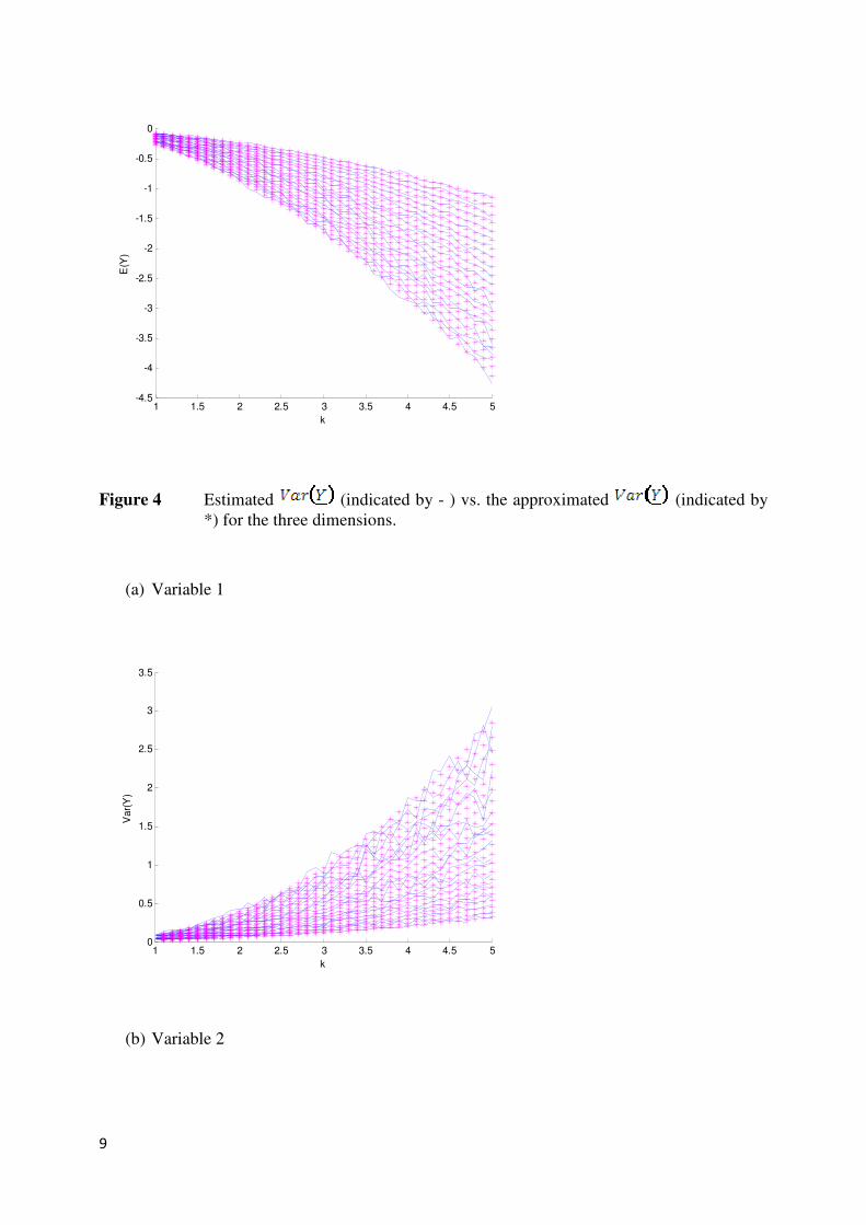
Figure 4 Estimated (indicated by - ) vs. the approximated (indicated by

*) for the three dimensions.

(a) Variable 1

1 1.5 2 2.5 3 3.5 4 4.5 50

0.5

1

1.5

2

2.5

3

3.5

k

Var(

Y)

(b) Variable 2

10

1 1.5 2 2.5 3 3.5 4 4.5 50

0.5

1

1.5

k

Var(

Y)

(c) Variable 3

1 1.5 2 2.5 3 3.5 4 4.5 50

0.5

1

1.5

2

2.5

3

3.5

k

Var(

Y)

For and the approximated mean and variance of are close to the estimated

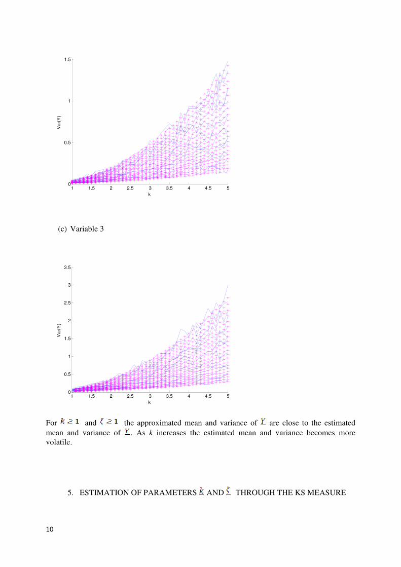
mean and variance of . As k increases the estimated mean and variance becomes more

volatile.

5. ESTIMATION OF PARAMETERS AND THROUGH THE KS MEASURE

11

This section discusses the estimation of the four MGBG parameters. The approach for

estimating the parameters and are the same as in the article of Beirlant et al. and are

estimated by first “trimming” the data, thus ignoring the extreme values, and then using the

method of moments to estimate and from the data below a threshold. The method of

moments are given by the following equations

( )1

1

ˆ ,..., '/tn

j pj t

j

y y nµ=

=∑

(5)

and

( ) ( )1

ˆ ˆ ˆ= ,..., ' , ..., ' / , 1,..., ; 1,...,tn

ij pj ij pj t t

j

y y y y n i p j nµµ=

Σ − = =

∑

(6)

where denotes the number of observations below the threshold . Thresholds are chosen

for each dimension by obtaining the 75th

upper quartiles as shown in Beirlant et al. (2000).

The Kolmogorov-Smirnov measure, (Conover, 1980) is then used to

estimate values for and where denotes the empirical cdf and the fitted cdf. Since it

is known that the Kolmogorov-Smirnov measure calculates the maximum

absolute difference between the empirical Gamma function and the cumulative Gamma

function for different values of and . With the KS measure one can see how well the

model fits the data. The minimum value of the different maximum KS measure values will

indicate the best fit.

6. SIMULATED DATA SETS

This section illustrates the estimation process as discussed in Section 5. values

were simulated from a MGBG with the following set of parameters,

. Figure 5

shows the simulated data values of . Let

.

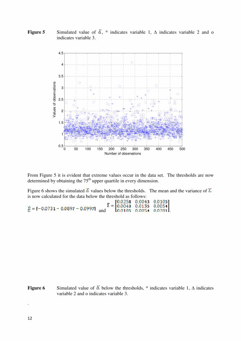
12

Figure 5 Simulated value of , * indicates variable 1, ∆ indicates variable 2 and ο

indicates variable 3.

0 50 100 150 200 250 300 350 400 450 5000.5

1

1.5

2

2.5

3

3.5

4

4.5

Number of observations

Valu

es o

f observ

ations

From Figure 5 it is evident that extreme values occur in the data set. The thresholds are now

determined by obtaining the 75th

upper quartile in every dimension.

Figure 6 shows the simulated values below the thresholds. The mean and the variance of

is now calculated for the data below the threshold as follows:

and .

Figure 6 Simulated value of below the thresholds, * indicates variable 1, ∆ indicates

variable 2 and ο indicates variable 3.

.

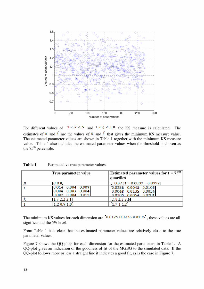
13

0 50 100 150 200 250 300

0.7

0.8

0.9

1

1.1

1.2

1.3

1.4

1.5

Valu

es o

f observ

ations

Number of observations

For different values of and the KS measure is calculated. The

estimates of and are the values of and that gives the minimum KS measure value.

The estimated parameter values are shown in Table 1 together with the minimum KS measure

value. Table 1 also includes the estimated parameter values when the threshold is chosen as

the 75th

percentile.

Table 1 Estimated vs true parameter values.

True parameter value Estimated parameter values for t = 75th

quartiles

The minimum KS values for each dimension are , these values are all

significant at the 5% level.

From Table 1 it is clear that the estimated parameter values are relatively close to the true

parameter values.

Figure 7 shows the QQ-plots for each dimension for the estimated parameters in Table 1. A

QQ-plot gives an indication of the goodness of fit of the MGBG to the simulated data. If the

QQ-plot follows more or less a straight line it indicates a good fit, as is the case in Figure 7.

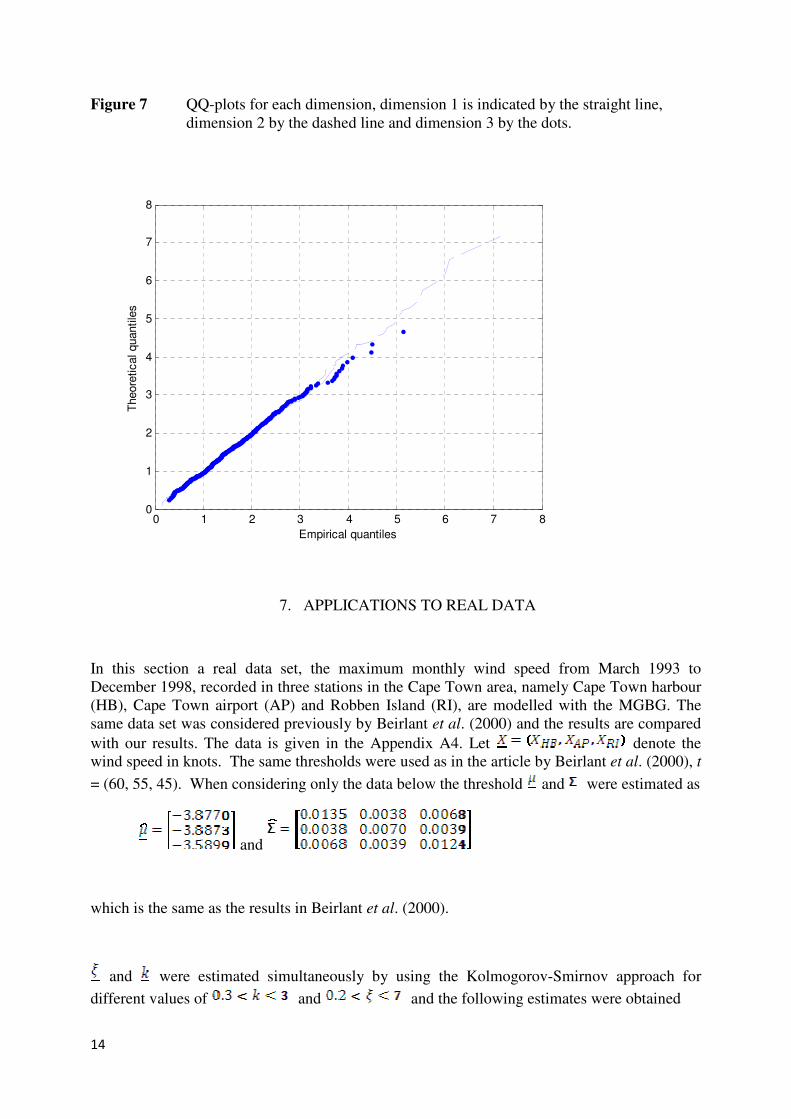
14

Figure 7 QQ-plots for each dimension, dimension 1 is indicated by the straight line,

dimension 2 by the dashed line and dimension 3 by the dots.

0 1 2 3 4 5 6 7 80

1

2

3

4

5

6

7

8

Empirical quantiles

Theore

tical quantile

s

7. APPLICATIONS TO REAL DATA

In this section a real data set, the maximum monthly wind speed from March 1993 to

December 1998, recorded in three stations in the Cape Town area, namely Cape Town harbour

(HB), Cape Town airport (AP) and Robben Island (RI), are modelled with the MGBG. The

same data set was considered previously by Beirlant et al. (2000) and the results are compared

with our results. The data is given in the Appendix A4. Let denote the

wind speed in knots. The same thresholds were used as in the article by Beirlant et al. (2000), t

= (60, 55, 45). When considering only the data below the threshold and were estimated as

and

which is the same as the results in Beirlant et al. (2000).

and were estimated simultaneously by using the Kolmogorov-Smirnov approach for

different values of and and the following estimates were obtained

15

and .

The estimates of and differs considerable from the estimates in Beirlant et al. (2000)

where and . QQ-plots with our parameters

and the parameters of Beirlant et al. (2000) are shown in Figure 8 for the different dimensions.

Figure 8 QQ-plots for each dimension, (*-) represents the QQ-plots with our parameters

and the (- -) represents the QQ-plots with the parameters of Beirlant et al.

(2000) and the solid line represents the 45o line.

(a) Dimension 1

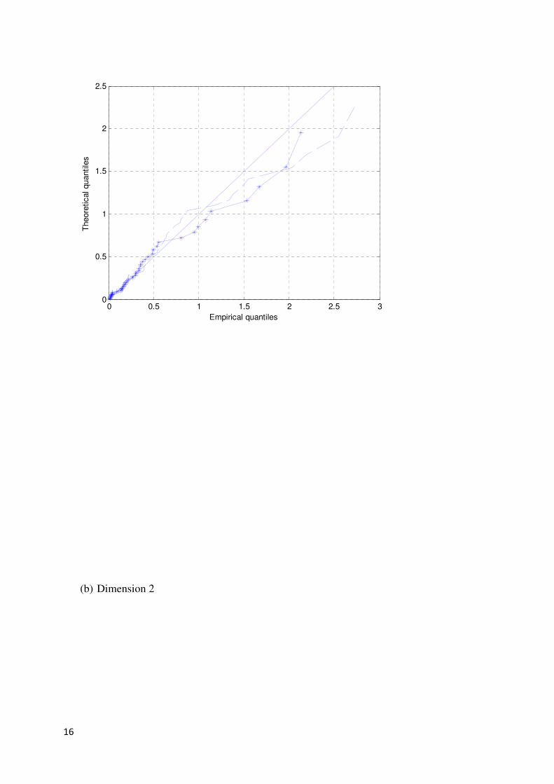
16

0 0.5 1 1.5 2 2.5 30

0.5

1

1.5

2

2.5

Empirical quantiles

Theore

tical quantile

s

(b) Dimension 2

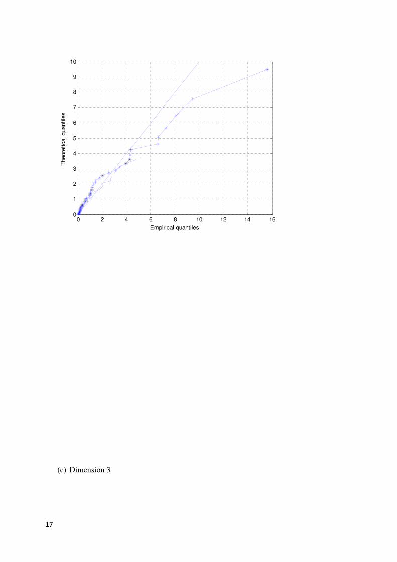
17

0 2 4 6 8 10 12 14 160

1

2

3

4

5

6

7

8

9

10

Empirical quantiles

Theore

tical quantile

s

(c) Dimension 3

18

0 2 4 6 8 10 120

1

2

3

4

5

6

7T

heore

tical quantile

s

Empirical quantiles

The line the closest to the 45o line will indicate the best fit. Although very similar, our model

seems to be closer to the 45o line in figures (a) and (c). A further test for goodness of fit is the

correlation coefficient rQ between the empirical quantiles and the theoretical quantiles. The

closer rQ is to 1 the better the fit (Beirlant et al. 2004, p.9). The rQ values are calculated as

follows:

Table 2 Calculated rQ values.

Our model Model of Beilant et al.

(2000)

Dimension 1 0.9895 0.9811

Dimension 2 0.9746 0.9856

Dimension 3 0.9797 0.9614

The correlation coefficients are high in both cases, although it is slightly higher in with our

model for dimensions 1 and 2.

8. CONCLUSION

19

The approach considered here for estimating the parameters of the MGBG seems to be

appropriate and easier than previously reported. It seems to be a slight improvement on the

estimation approach considered in Beirlant et el. (2000). Further research can be done in

perhaps considering a thoroughly Bayesian approach for estimating all four parameters

simultaneously.

APPENDIX

A.1:

The expected value of , 1,...,i

X i p= , where ( ) ( )1

log 1 ,1~GAMi i i i

i

V V kξ ξξ

= + is given by the

approximation

( ) ( ) ( )21exp exp

2i i ii Y Y YE X µ σ µ≈ − + − .

(a.1)

Proof:

From (a.1) 1i i

V

i

i

eV

ξξ

ξ

−= , therefore ( )

1log log

i iV

i

i

eE E V

ξξ

ξ

−=

.

To obtain the ( )logi

E V the delta method given by Rice (1995, p. 149) is used. This method

involves the expansion of the Taylor series to the second order to improve the approximation.

Therefore ( )( ) ( ) ( )21log

2i i ii V V VE V g g

ξ ξ ξµ σ µ′′≈ + ,

where

i

V ik

ξµ = ,

2

iV ik

ξσ = ,

( )i

Vgξ

µ = 1

log

i Vi

i

e ξξ µ

ξ

−

,

20

( )1

i Vi

i Vi i

i

V

eg

e

ξ

ξ ξ

ξ µ

ξ µ

ξµ′ =

−

and

( )( )

2

2

1

i Vi

ii V

i

iV

eg

e

ξ

ξξ

ς µ

ξ µ

ξµ

−′′ =

−

.

Therefore

( )( )( )

2

2

1log log

2 1

i ii i

i i

kk

i i

ik

i

k eeE V

e

ξ

ξ

ξ

ξ

ξ −≈ −

−.

(a.2)

The delta method also indicates that ( ) ( )( )2

2logi i

i V VVar V g

ξ ξσ µ′≈ , therefore

( )2

log1

i i

i i

k

i

i i k

eVar V k

e

ξ

ξ

ξ ≈

− .

(a.3)

From (2) ( )logi iY X= − , therefore ( ) ( )expi i iX g Y Y= = − , where

21

( )

( )

( ) ( )

( ) ( )

1 1

1

1

12

1 1

12

1log

.

.

.

1log

log

.

.

.

log

1

1

=

p p

V

i i i

V

p

p

i i

p p

ek

Y D

ek

V k

D

V k

ξ

ξ

ξ

ψ

ξ

ψ

ψξ

µ

ψξ

ψ

µ

ψ

−

−

−−

= −∑ + − −

−

−∑ + −

(a.4)

and

( ) ( ) ( )( )1 2, ,..., .diag pD k k kψ ψ ψ ψ′ ′ ′=

(a.5)

Again the delta method is used to obtain an approximation for ( )iE X (Rice 1995, p. 149).

Thus, when following the delta method, the following is obtained:

( ) ( ) ( )

( ) ( ) ( ) ( )

21,

2

exp exp .

i i ii Y Y Y

i i i i

E X g g

g Y Y g Y Y

µ σ µ′′≈ +

′ ′′= − − = − and

(a.6)

Therefore

( ) ( ) ( )21exp exp

2i i ii Y Y YE X µ σ µ≈ − + −

(a.7)

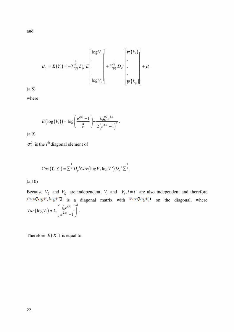
22

and

( ) ( ) ( )

( )

( )

11

1 1

1 12 2

log

. .

. .

. .

log

iY i ii i

p p

kV

E Y D E D

V k

ψ ψ

ψ

µ µ

ψ

− −

= = −∑ + ∑ +

(a.8)

where

( )( )( )

2

2

1log log

2 1

i ii i

i i

kk

i ii

ki

k eeE V

e

ξξ

ξ

ξ

ξ

−≈ −

−.

(a.9)

2

iYσ is the ith

diagonal element of

( ) ( )1 1

1 12 2, ' log , log 'Cov Y Y D Cov V V Dψ ψ− −= ∑ ∑ .

(a.10)

Because i

Vξ and 'i

Vξ are independent, iV and ' , 'iV i i≠ are also independent and therefore

is a diagonal matrix with on the diagonal, where

( )log1

i i

i i

k

ii i ki

eVar V k

e

ξ

ξ

ξ ≈

−

2

.

Therefore ( )iE X is equal to

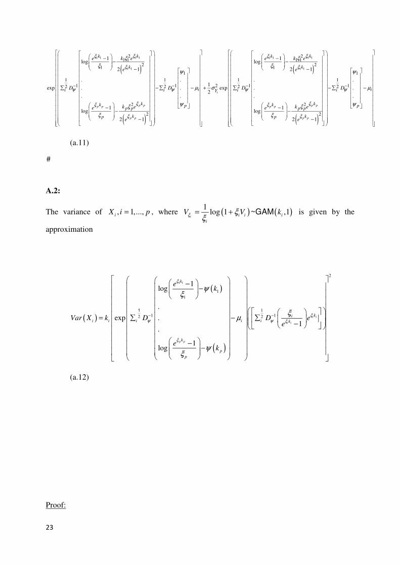
23

( )

( )

1 11 1

1 1

21 1

21

1

1 1

1 12 2

2

2

1log

2 1

. .

exp . .

. .

1log

2 1

p pp p

p p

kk

k

ii i

kk pp p

kp

k ee

e

D D

k ee

e

ξξ

ξ

ψ ψ

ξξ

ξ

ξ

ξψ

µ

ψξ

ξ

− −

− −

− ∑ −∑ − − − −

( )

( )

1 11 1

1 1

21 1

21

1

1 1

2 1 12 2

2

2

1log

2 1

. .1

exp . .2

. .

1log

2 1

i

p pp p

p p

kk

k

i iY

kkp p

kp

k ee

e

D D

k ee

e

ξξ

ξ

ψ ψ

ξξ

ξ

ξ

ξψ

σ

ξ

ξ

− −

− −

−

+ ∑ −∑ − −

−

i

p

µ

ψ

−

(a.11)

#

A.2:

The variance of , 1,...,iX i p= , where ( ) ( )1

log 1 ,1~GAMi i i i

i

V V kξ ξξ

= + is given by the

approximation

( )

( )

( )

1 1

2

1

1

1

1 12 2

1log

.

exp .1

.

1log

i i

i i

p p

k

ki

i i i i i k

k

p

p

ek

Var X k D D ee

ek

ξ

ξψ ψ ξ

ξ

ψξ

ξµ

ψξ

− −

− − = ∑ − ∑ − − −

1

(a.12)

Proof:

24

From A.1 iY is defined as

( ) ( )

( ) ( )

1 1

12

log

.

.

.

log

1

= i i i

p p

V k

Y D

V k

ψ

ψ

µ

ψ

−

−

−∑ + −

.

In A.1 it was shown that ( )exp , 1,...,i iX Y i p= − = , therefore

( )

( )

( )

1 1

1

1

1

12

1log

.

exp .

.

1log

,..., .

p p

p

V

i i i

V

p

p

ek

X D

ek

g V V

ξ

ξ

ξ

ψ

ξ

ξ ξ

ψξ

µ

ψξ

−

− − = ∑ − − −

=

1

(a.13)

When applying the delta method

( ) ( )( )

i

ii i

i

V

i V V

gX g V

V

ξ

ξ ξξ

ξ

µµ µ

∂≈ + −

∂.

(a.14)

Now it follows that:

( ) ( )( )

2

i

i

i

V

i

gVar X Var V

V

ξ

ξ

ξ

µ ∂ ≈ ∂

.

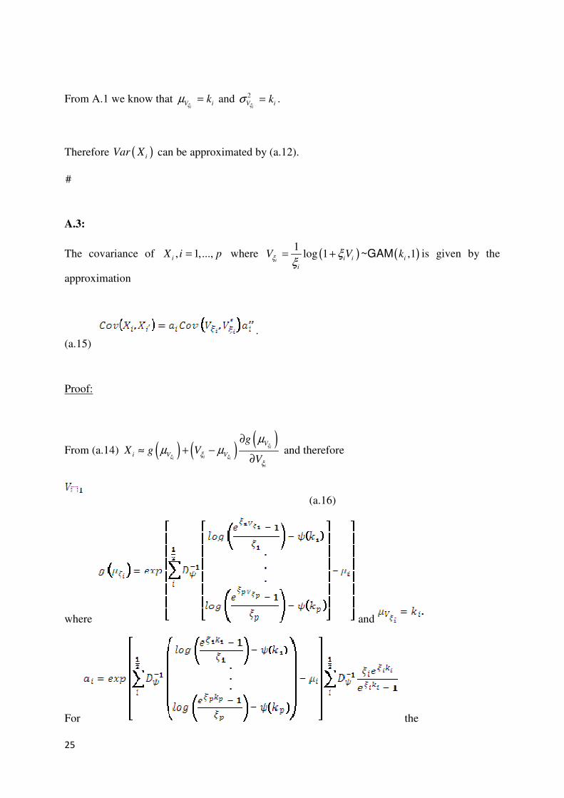
25

From A.1 we know that i

V ik

ξµ = and 2

iV ik

ξσ = .

Therefore ( )iVar X can be approximated by (a.12).

#

A.3:

The covariance of , 1,...,iX i p= where ( ) ( )1

log 1 ,1~GAMi i i i

i

V V kξ ξξ

= + is given by the

approximation

.

(a.15)

Proof:

From (a.14) ( ) ( )( )

i

ii i

i

V

i V V

gX g V

V

ξ

ξ ξξ

ξ

µµ µ

∂≈ + −

∂ and therefore

(a.16)

where and

For the

26

.

(a.17)

Because i

Vξ and 'i

Vξ are independent, is a diagonal matrix with in

the diagonal.

#

A4:

Maximum monthly wind speed data measured at Cape Town Harbour, Cape Town Airport and

Robben Island, from March 1993 to December 1998.

Harbour Airport Robben Island

121 45 35

49 56 37

39 41 27

41 45 35

56 60 39

56 47 37

39 49 41

49 43 37

53 47 39

53 49 43

51 47 39

51 47 39

47 43 39

60 45 37

45 45 37

89 70 53

49 54 39

43 45 43

41 45 33

43 39 31

43 45 33

47 47 37

56 51 37

49 43 35

62 41 35

51 47 64

136 51 33

70 56 45

27

89 51 33

58 45 41

41 45 31

54 54 45

45 47 37

54 53 41

54 49 39

49 51 31

53 47 35

49 47 31

37 45 29

51 64 41

47 49 33

97 49 41

47 53 37

56 47 41

53 51 41

51 53 37

53 49 37

58 51 39

54 45 37

47 39 41

49 47 31

58 70 45

37 43 33

72 51 41

53 45 45

45 45 37

43 49 37

56 54 41

54 51 39

54 49 39

49 45 33

47 37 29

51 47 39

43 41 29

43 47 39

45 47 35

51 47 33

49 41 37

53 43 39

54 43 39

REFERENCE

[1] Beirlant J, De Waal DJ & Teugels JL. 2000. A Multivariate Generalized Burr-Gamma

Distribution. South African Statistical Journal 34: 111-133.

28

[2] Beirlant J, De Waal DJ & Teugels JL. 2002. The generalized Burr-Gamma family of

distribution with applications in extreme value analysis. Limit Theorems in Probability

and Statistics I: 113-132.

[3] Beirlant J, Goedgebeur Y, Segers J & Teugels J. 2004. Statistics of Extremes Theory

and Applications; Wiley & Sons: England.

[4] Conover WJ. 1980. Practical Nonparametric Statistics. Second Edition; Weily & Sons:

United States of America.

[5] Meng XL. 1997. The EM algorithm and medical studies: a historical link. Statistical

Methods in Medical Research 6: 3-23.

[6] Rice JA. 1995. Mathematical Statistics and Data Analysis. Second edition; Duxbury

Press: California.

[7] Salisbury JI & Wimbush M. 2002. Using modern time series analysis techniques to

predict ENSO events from the SOI time series. Nonlinear Processes in Geophysics 9:

341-345.

1

Semi-Parametric Inference for Measures of Inequality (Preliminary Report)

Tertius de Wet1

tdewet@sun.ac.za

Stellenbosch University

Abstract

In this paper we discuss the semi-parametric estimation of measures of inequality, in

particular, the Gini measure. This estimation procedure is specifically applicable in

the case of heavy tailed distributions. Such distributions often occur in real data sets

e.g. in income data which usually have a heavy right tail. The estimation is illustrated

by application to the South African Income and Expenditure data of 2005.

1. Introduction.

Measures of inequality, also called measures of concentration or diversity, are very

popular in economics and especially in measuring the inequality in income or wealth

within a population and between populations. However, they have applications in

many branches of science, e.g. in ecology (Magurran, 1991), linguistics (Herdan,

1966), sociology (Allison, 1978), demography (White, 1986) and information science

(Rousseau, 1993).

Over the years a large number of measures have been proposed, with the Gini index

perhaps the most well-known one. Having reliable inequality measures available is an

important first step. A next step is to estimate the values of these measures using

samples from the appropriate populations and, in particular, to estimate the variability

of these estimators and more generally, to obtain confidence intervals for the

measures. Since inequality is inherently dependent on the tails of a population,

estimators of inequality are typically sensitive to data from these tails. We note in this

regard that all the well-known inequality measures have unbounded influence

functions. It is well-known that income distributions often exhibit a long tail to the

right, making estimators of inequality particularly sensitive to large values. It is thus

important to study the behaviour of estimators based on data from heavy tailed

distributions. Many of the traditional estimators are sensitive to such extreme data

points (see e.g. Cowell and Flachaire, 2007) and remedial action needs to be taken.

This remedial action can be either a trimming of the extreme data or a modification of

the estimator to make it more robust to extreme observations.

Cowell and Flachaire (2007) (see also Cowell and Victoria-Feser, 2008) have

proposed a so-called semi-parametric approach to modify estimators under heavy

tailed distributions. This method estimates the left part of the distribution, where the

bulk of the distribution resides, using the usual nonparametric empirical distribution

function and the right (upper) part of the distribution using a parametric extreme value

distribution, e.g. a Pareto distribution. The resulting estimator is therefore partly

nonparametric and partly parametric, hence semi-parametric. Results from extreme

value theory are then used to obtain a more reliable distribution estimator. This new

estimator of the distribution forms the basis for more robust estimators of the

measures of inequality. Since these new estimators are expected to have a limiting

1 This paper is based on joint work with Tchilabalo Kpanzou and Ariane Neethling, both from Stellenbosch

University.

2

normal distribution, approximate confidence intervals can be obtained using standard

normal theory.

In this (preliminary) report we build on these ideas and focus, in particular, on the

Gini index for illustrative purposes. It is shown how results from extreme value theory

can be used to find an appropriate parametric distribution to use, also leading to a

choice of the number of observations to use in fitting this parametric distribution. The

results are applied to a well-known South African income data set, the IES 2005.

The layout of the paper is as follows. In the next section a number of measures of

inequality are discussed, in Section 3 the approach to semi-parametric estimation of

the Gini index is discussed and in Section 4 the results are applied to the IES 2005

data set. A number of further aspects being investigated are discussed in the closing

section.

2. Measures of Inequality.

A large number of measures of inequality have been proposed in the literature. We

discuss the two most important ones, viz. the generalized entropy (class of) measures,

which includes the Theil and mean logarithmic deviation, and the Gini measure. In

addition, we discuss a more recent proposal, the quintile share ratio. Our focus for this

paper will be on the Gini inequality measure.

Let Y denote the random variable of interest and suppose Y is positive valued and has

a distribution function F .

2.1 Generalized Entropy Measures

The generalized entropy (GE) measure is defined by (see e.g. Cowell and

Flachaire, 2007)

( ) ( ) ( ) ( ) ( )1 1

0

1 1 1 1 ,y

EI dF y α

αα υ

µ µα α α α

∞− − = − − = − − ∫

where

( ) ( )0 0

, and ydF y y dF y Rαµ υ α

∞ ∞

= = ∈∫ ∫ .

It follows quite easily that the influence function of E

Iα is given by

( ) ( )[ ]11

; EIF z I z zα

α α υ

α µυ µ+−

= − − − .

Clearly the influence function is unbounded when z → ∞ .

Two special cases of the GE measure are the Theil measure, when 1α = , i.e. 1 logEI υ

µµ= − ,

where now ( )0

logy ydF yυ∞

= ∫ ,

and the mean logarithmic deviation, when 0α = , i.e.

( ) ( )0

0

log logy

EI dF y

µµ υ

∞

= = −∫ ,

where now ( )0

log ydF yυ∞

= ∫ .

2.2 Gini Index

The Gini index is the most widely used measure of inequality. There are a number

of different ways of defining it, the most well-known the following.

3

Let

( ) ( ) ; inf :Q q F y F y q≡ ≥

denote the quantile function of F ,

( ) ( ) ( )( );

0 0

; ;

Q q Fq

C q F Q u F du ydF y≡ =∫ ∫ ,

the cumulative quantile function and

( )0

ydF yµ∞

= ∫ ,

as before.

The Gini index is then given by

( ) ( )1

1

0

1 2 ; 1 2G

I C u F du R Fµ −≡ − ≡ −∫ ,

with

( ) ( )1

1

0

;R F C u F duµ −= ∫ .

Remark. The Gini index is closely related to the Lorenz curve. The latter is

defined as

( ) ( );;

C q FL q F

µ≡ .

Thus

( )1

0

1 2 ;G

I L u F du= − ∫ ,

i.e. one minus twice the area under the Lorenz curve. Furthermore

( ) ( )( )1 1 1

0 0 0

2 ; 2 ;GI udu L u F du u L u F du

= − = − ∫ ∫ ∫ .

This shows that the Gini index is twice the area between the 45 degree line and the

Lorenz curve.

The influence function of the Gini index is easily seen to be

( ) ( ) ( )( ) ( ) ( )( )( ); 2 ; 1zGIF z I R F C F z F R F F z

µ = − + − − ,

which tends to infinity at the rate of z when z → ∞ .

A number of alternative definitions of the Gini index are as follows.

(i) 11 22

| |G

I E Y Yµ

= − ,

where 1 2 and Y Y are independent random variables each having distribution

F .

(ii) The expression in (i) can also be written as

4

( ) ( )1 1

12

0 0

| ; ; |G

I Q u F Q v F dudvµ

= −∫ ∫ .

(iii) ( )( )2

1

0

1 1G

I F y dyµ

∞

= − −∫ .

Note that this can also be written as

( )( ) ( ) ( )( )2 11

0 0

1 1 1G

I F y dy F y F y dyµ

µ∞ ∞

−= − − = −∫ ∫ .

Remark. Note that the Gini index lies between zero and one, with zero indicating

perfect equality and one indicating perfect inequality.

2.3 Quintile Share Ratio Measure

This measure is defined as the ratio of the 0.8th

quantile to the 0.2th

quantile, i.e.

( ) ( )0.8; / 0.2;QSR Q F Q F= .

Remark. This measure forms part of the so-called Laeken indicators, the

European indicators on poverty and social exclusion. We only mention this

measure and will not discuss it further.

3. Semi-parametric estimation for the Gini index.

Consider now the Gini index as given in (iii) in the previous section:

( ) ( )( )1

0

1G

I F y F y dyµ∞

−= −∫ .

Given a sample 1,..., nY Y of size n on Y , the usual nonparametric estimator for

GI is

given by

( ) ( )( )1

0

1NP

G n n nI F y F y dyµ

∞−

= −∫ɵ ,

where

( ) ( )1

1

n

n i

i

F y n I Y y−

=

= ≤∑

is the empirical distribution function and

1

1

n

n i

i

n Yµ −

=

= ∑

is the sample average.

In many cases the distribution function F has a heavy right tail, with relatively fewer

observations in the tail part of the distribution. In such a situation it may not be wise

to use the empirical distribution function to estimate F over its whole range. A better

choice might be to use n

F to estimate F over the bulk of the data, but to use a

parametric estimator in the tail part of F . This was the approach suggested by Cowell

and Flachaire (2007) (see also Cowell and Victoria-Feser, 2008). Since it is assumed

that F has a heavy right tail, extreme value theory can be used. In this section such an

approach will be followed.

Now, define a semi-parametric distribution function by

( )( )

( ) ( )( ) ( )

0

0

,

1 ,

F y y yF y

F y F y F y y yθ

≤=

+ − >

5

for a given 0y , where Fθ is derived from some parametric distribution (e.g. Pareto or

generalized Pareto). The distribution function F can be thought of as the unknown

underlying distribution function that will be estimated (in the bulk of the data) by the

empirical distribution function.

Taking 0y as an upper quantile of F , say ( )0 1 ;y Q Fα= − , leads to

( )( ) ( )

( )( ) ( )

, 1 ;

1 1 , 1 ; .

F y y Q FF y

F y y Q Fθ

α

α α

≤ −=

− − > −

The semi-parametric Gini index is given by

( ) ( )( )1

0

1SPG

I F y F y dyµ∞

−

= −∫ .

We now give a simplified expression for SPG

I that will be used in deriving an

estimator for it.

First, note that

( )( )

( )( )( )

( )( )( )

0

1 ;

0 1 ;

1

1 1

Q F

Q F

F y dy

F y dy F y dy

α

θ

α

µ

α

∞

− ∞

−

= −

= − + −

∫

∫ ∫

and

( ) ( )( )

( ) ( )( )( )

( )( ) ( )( )( )

1

0

1 ;1

0 1 ;

1

1 1 1 1 .

SPG

Q F

Q F

I F y F y dy

F y F y d y F y F y dy

α

θ θ

α

µ

µ α α

∞−

− ∞−

−

= −

= − + − − −

∫

∫ ∫

On the interval ( )( )0, 1 ;Q Fα− we estimate F by the empirical distribution function

.n

F

Now, denote the order statistics of the sample by 1, 2, ,...n n n n

Y Y Y< < < and let kn

α =

for some appropriately chosen integer k . Then ( )1 ;Q Fα− can be estimated by ,n k nY − .

On the interval ( )( )1 ; ,Q Fα− ∞ we want to use a parametric distribution obtained

from extreme value theory. This approach is now briefly described.

Write GPD for the generalized Pareto distribution and GEV for the generalized

extreme value distribution. It is then well known (see e.g. Beirlant et al., 2004) that

for a threshold u

( )| , for large D Y u Y u GPD u− > ≐ ,

whenever Y lies in the domain of attraction of the GEV.

Therefore, if G denotes the GPD, we can write

[ ] [ ] [ ]

( ) ( )

( )

| /

/

,

P Y u y Y u P Y u y P Y u

F y u F u

G y

− > > = − > >

= +

≈

where ( ) ( )1F y F y= − and ( ) ( )1G y G y= − .

6

It follows that

( ) ( ) ( )F y u F u G y+ ≈ ,

which becomes (by letting y u y+ → )

( ) ( ) ( )F y F u G y u≈ − and

( ) ( ) ( )1F y F u G y u≈ − − .

The right hand side of this is then the ( )F yθ in the semi parametric form above.

Remark. Note that the GPD has two unknown parameters, say γ and σ . The form of

G is then

( )1/

1 1 xG xγ

σγ

−= − + .

The parameters γ and σ can be estimated by maximum likelihood. See Beirlant et al.

(2004).

We now give an estimator for SPG

I by estimating the elements in its expression given

above.

Note that, as mentioned above, if we take kn

α = then ( )1 ;Q Fα− can be estimated by

,n k nY − . Therefore, for ,n k n

y Y −≤ we estimate F by

( ) ( )n nF y F y= ,

the empirical distribution function.

Consider now ,n k ny Y −> and let ( ), 'θ γ σ≡ , the GPD parameter and write ɵθ for the

corresponding maximum likelihood estimator.

Writing G Gθ≡ to indicate the dependence on the unknown parameter, we estimate it

by ɵ

Gθ

. Using the above approximation for ( )F y for a large threshold, for ,n k ny Y −>

we estimate F by

( ) ɵ ( )( ),1 1 1k kn n k nn n

F y G y Yθ −

= − − − −

.

Here, with the threshold u taken as ,n k nY − , the estimator for ( )F u is taken as

( ),1 kn n k n n

F Y −− = .

Putting this together, gives the final estimator as

( )( )

ɵ ( )( ),

, ,1 1 1 .

n n k n

n k kn k n n k nn n

F y for y Y

F yG y Y for y Y

θ

−

− −

≤

= − − − − >

Substituting this in SPG

I , gives our estimator SPGIɵ . The following result gives a

convenient computational formula for this estimator.

Theorem. The estimator SPGIɵ can be written as

( ) ( )( ) ɵ ( ) ɵ( ) ɵ( )1

2 2 2 2 2 4

, 1,

1

1 2 / 1 2n k

iSPG i n i nn

i

I n i Y Y k n k n k nµ σ γ µ γ γ−−

−

=

= − − + − − − − − ∑ɵ ,

7

where ɵγ and σ are the maximum likelihood estimators and µ can be calculated as

( )( ) ɵ( ) ɵ2 2

, 1, 0,

1

1 / 1 , 0, 1.n k

ii n i n nn

i

Y Y k n Yµ σ γ γ−

−

=

= − − + − = <∑ .

Remark. As is usual in extreme value theory, the choice of the threshold u to work

with, or equivalently the choice of the number of exceedances k , is of critical

importance. In our application we will apply a goodness-of-fit test to test for the GPD

and choose k as the value that gives a reasonable p value. The goodness-of-fit test

used will be based on the work of Choulakian and Stephens (2001) and Villasenor-

Alva and Gonzalez-Estrada (2009).

4. Results for IES 2005.

We apply the proposed method to the variable EQ_INC (Equalized Income) of the

South African Income and Expenditure Survey data (IES2005), consisting of 20 986

observations. The data ranges from 0 to 2 910 826.00, with a heavy right tail as

shown by the histogram below.

Applying the GPD test (as discussed in Choulakian and Stephens, 2001 and

Villasenor-Alva and Gonzalez-Estrada, 2009) to the exceedances, we found a p-value

of ˆ 0.78p = for 630k = (3% of the data). The estimates of the shape and scale

parameters for the GPD are respectively given by ˆ 0.6402γ = and ˆ 45053.7500σ = .

The corresponding semi-parametric Gini index is estimated by ˆ 0.6154SPG

I = . The

nonparametric estimate of the Gini index is given by ˆ 0.6703G

I = .

5. Further work.

This is a preliminary report on a research project that has only recently started.

Clearly there are still many outstanding issues to explore. Below some of these are

mentioned that are currently being investigated.

• If instead of the exceedances Y u− , relative exceedances /Y u are

considered, then it is well known that

( )/ | , for large D Y u Y u Pareto u> ≈ .

One can thus carry out the program above for the Pareto distribution rather

than the GPD. Furthermore, a second order approximation exists for such

exceedances, viz. approximation by the so-called perturbed Pareto distribution

(PPD). This should give a better fit in the tail of the distribution.

• The influence functions of the measures of inequality considered are clearly

sensitive to outlying values. What is the effect of outliers on the semi-

parametric estimators? How should this effect be countered, e.g. through

appropriate trimming?

• The above was illustrated only for the Gini measure. Similar results are being

derived for other measures of inequality.

• Estimating a measure of inequality is only a first step. The next step would be

to obtain confidence intervals. This is being carried out in different ways.

- Using a re-sampling method such as the bootstrap.

8

- Using asymptotic theory. Since these estimators are asymptotically

normally distributed this is fairly straightforward. However, results may

not be accurate for “small” samples.

- In order to improve small sample accuracy of the confidence intervals, use

could be made of transformations. Some work in this direction has

recently been done by Schluter and van Garderen (2009).

• Survey data is often based on complex sampling schemes. How can the semi-

parametric approach be modified to accommodate such data?

6. References.

Allison P.D. (1978). Measures of inequality. American Sociological Review 43, 865 –

880.

Beirlant J., Goegebeur Y., Segers J. and Teugels J. (2004). Statistics of Extremes:

Theory and Applications. Wiley, New York.

Choulakian V. and Stephens M.A. (2001). Goodness-of-Fit Tests for the Genaralized

Pareto Distribution. Technometrics 43, 478 – 484.

Cowell F.A. and Flachaire E. (2007). Income Distribution and Inequality

Measurement: The Problem of Extreme Values. Journal of Econometrics 141, 1044 –

1072.

Cowell F.A. and Victoria-Feser M-P. (2008). Modelling Lorenz Curves: Robust and

Semi-Parametric Issues. In Duangkomen Chotikapanich (editor) Modelling Income

Distributions and Lorenz Curves, 241 – 253. Springer.

Herdan G. (1966). The Advanced Theory of Language as Choice and Chance.

Springer.

Rousseau R. (1993). Measuring Concentration: Sampling design issues, as illustrated

by the case of perfectly stratified samples. Scientometrics 28, 3 – 14.

Schluter C. and van Garderen K.J. (2009). Edgeworth Expansions and Normalizing

Transforms for Inequality Measures. Journal of Econometrics 150, 16 – 29.

Villasenor-Alva J.A. and Gonzalez-Estrada E. (2009). A Bootstrap Goodness of fit

Test for the Generalized Pareto Distribution. Computational Statistics and Data

Analysis 53, 3835 – 3841.

White M.J. (1986). Segregation and Diversity Measures in Population Distribution.

Population Index 52, 198 – 221.

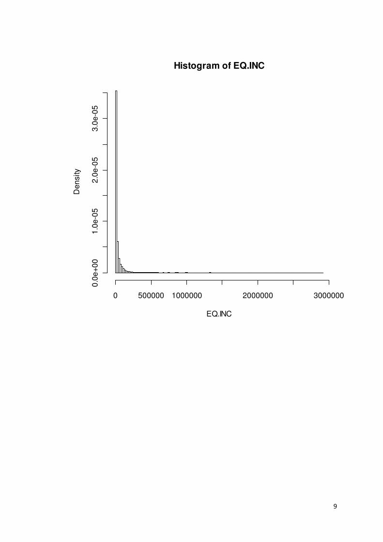
9

Histogram of EQ.INC

EQ.INC

De

nsity

0 500000 1000000 2000000 3000000

0.0

e+

00

1.0

e-0

52

.0e

-05

3.0

e-0

5

AN APPLICATION OF SEQUENTIAL REGRESSION MULTIPLE IMPUTATION ON PANEL

DATA

MICHAEL JOHAN VON MALTITZ

ABRAHAM JOHANNES VAN DER MERWE

1. INTRODUCTION

One of the major issues associated with large surveys is that of non-response or lost data. Moreover, the main

problematic issue regarding missing data is that most data analysis procedures are not designed to handle

them, leading to analyses that conclude invalid and inefficient inferences about a population (Schafer and

Graham, 2002). Many economic analyses use either complete-case analysis or a simple but inaccurate method

of imputing missing data. In most cases, the missing data is multivariate, meaning that missing values appear

in several observed variables. In essence, we have that a complete data matrix Y is made up of an

observed part, Y, and a missing part, Y. The data that is missing has a particular distribution of positions.

These positions are indicated by a matrix R of zeroes and ones that has the same dimensions as the complete

data matrix Y. In R there are ones in the positions of the missing data entries of Y, and zeroes

elsewhere. The distribution of R, referred to as the distribution of ‘missingness’, is P(R|Y, ), where ξ is a

vector of unknown parameters.

There are three mechanisms by which data is said to be missing – ‘missing at random’ (MAR), ‘missing

completely at random’ (MCAR), or ‘missing not at random’ (MNAR). In the MAR mechanism, the distribution

of positions of the missing data entries is assumed to be independent of the missing data in the analysis, or

P(R|Y, = P(R|Y, . In the case of MCAR, a special version of the MAR mechanism, the positions of

the missing data entries are assumed to be independent of all of the variables in the analysis, i.e.

P(R|Y, = P(R| . In the last case, the MNAR missing data mechanism, the positions of the missing data

entries are assumed to be at least dependent on data that is missing from the dataset, or, more basically, the

distribution of missingness is not MAR. This means that for MNAR, P(R|Y, ≠ P(R|Y, . If the

mechanism behind the missing data is MAR, then the mechanism is said to be ‘ignorable’ (Little and Rubin,

1987).

In complete-case analysis, only cases containing values for each of the variables in question are retained in

the data analysis procedures. This can raise the problem of serious bias in the analysis (Little and Rubin, 1987).

One must note, however, that these possible biases may not always exist in complete-case analysis, but rather

that the extent of bias will depend on the mechanism by which data is deemed to be missing. Particularly, if

the data is MCAR, then there will be no bias in complete-case analysis of multivariate data with missing

entries (Schafer, 2003). To overcome the possible biases in complete-case analysis, many methods of dealing

with incomplete data and imputing missing values have been suggested. The non-imputation methods of

handling incomplete data include available-case analysis, weighting procedures or model-based procedures.

Alternatively, if complete-case analysis methods are to be used on a dataset that is originally incomplete, data

can be ‘filled in’ by several imputation procedures, including substitution, cold-deck imputation, unconditional

and conditional mean substitution, imputation from unconditional distributions or hot-deck imputation, and

imputation from conditional distributions. All of these imputation procedures are single imputation methods,

imputing only one value for each missing datum.

Multiple imputation, also proposed by Rubin (1987), is viewed as a flexible alternative to likelihood methods

for a range of incomplete data problems (Schafer and Graham, 2002). The primary advantage of multiple

imputation is the inflation of uncertainty in the analysis estimates. In essence multiple imputation covers a

class of methods that impute several plausible values for a single missing data entry. Once the missing values

have been imputed, several completed datasets are left to be analysed by complete-case methods. A simple

set of rules is then used to combine the estimates from the separate analyses of the several datasets, and the

uncertainty of these estimates is then formed from the sample variation as well as variation in the imputed

values themselves. Although the number of datasets that should be completed is often debated, a small

number of completed datasets, say, between 10 and 20, often suffices in order to obtain precise estimates.

Multiple imputation can be easily linked to Bayesian statistics, as the imputed values for a single missing data

entry can be draws from the predictive posterior distribution for the non-missing data. One relatively new

method of imputation is that of Raghunathan et al. (2001), namely sequential regression multiple imputation,

or SRMI. This method extends and refines imputation from conditional distributions into a multiple

imputation context. The process will be detailed in the methodology section.

2. METHODOLOGY

2.1 Hypothesis

The hypothesis of interest is that there are no changes in the parameters of a regression analysis once

imputation has been performed using the SRMI process. More accurately, we want to determine whether or

not social networks have influenced welfare in South Africa. The research problem is quite simply linked to

this hypothesis. If there are changes in the parameters of interest from before imputation to after imputation,

then the researcher has to decide which set of parameters, if any, will be used to aid policy decision. The

problem to be solved is the adequacy of whichever estimates are decided on.

2.2 Data

This research uses the combined datasets of the Project for Statistics on Living Standards and Development

(PSLSD), undertaken in 1993, and the follow up KwaZulu-Natal Income Dynamics Study (KIDS) surveys

undertaken in 1998 and 2004.1 These two studies form a three-period panel data set of 1412 households in

1993, 1075 households in 1998, and 1428 households in 2004. Once data constraints have been taken into

account, the household models include 1158 African and Indian households. These figures are calculated

before cases are dropped in any complete-case analysis on the data. Additionally, since the 1993 survey was

designed to be self-weighted, it may only be assumed that the 1998 sample of households is representative of

the 1993 population, as is the sample in 2004. The data actually spans 3928 observations in 1906 households

when the survey waves are combined in a single dataset. If a complete-case random effects regression is

performed on this data, 1600 cases are dropped before the analysis is completed. This is a large number

relative to the number of households available for analysis, meaning that the complete-case procedures may

produce severely biased results if the data is not MCAR.

2.3 Multiple Imputation through Sequential Regression

Raghunathan et al. (2001: 85) summarize the SRMI process for a single cross-sectional dataset:

1 The KwaZulu-Natal Income Dynamics Study (KIDS) was a collaborative project of the International Food Policy Research

Institute, the University of Natal-Durban, the University of Wisconsin-Madison, and the Southern Africa Labour and

Development Research Unit at the University of Cape Town. The 2004 data used in the analysis was generously provided

by the KIDS research team before the public release of the data. This means that the data had yet to be cleaned. Even

though extensive cleaning of the data was required, in particular for individual’s ages, education levels, household heads,

and even gender, the cleaning was approached with much care, so as to preserve the validity of the data.

“This approach specifies an explicit model for variables with missing values, conditional on the fully

observed variables and some unknown parameters, and a model for the missing data mechanism,

which does not need to be specified under an ignorable missing data mechanism (Rubin, 1976). This

explicit model then generates a posterior predictive distribution of the missing values conditional on

the observed values. The imputations are draws from this posterior predictive distribution.”

Firstly, the dataset’s incomplete variables are sorted from the variable with the least missing entries to the

variable with the most missing values. Let the variable with the least missing be , the variable with the next

fewest missing be , etc., until . Let X be that part of the dataset that is originally complete. Finally, let

be a vector of the unknown regression and dispersion parameters in the conditional model for . The sorting

of the dataset follows as an extension to the fact that in model-based imputations the joint conditional

density of , , … , given X can be factored as

(, , … , |X, , , … ,

= (|X, ( |X, , … (|X, , , … , , (1.1)

Each conditional density is modelled by an appropriate regression model with unknown parameters, .

Secondly, the first round of imputations begins, and the variable with the least missing data entries (apart

from the complete variables) is selected. This variable is regressed on the complete data according to a

regression model that is assumed to fit the distribution of the variable, as mentioned above. The model first

processed is illustrated in Equation (2.1) by . The regression is Bayesian by nature, but utilizes a diffuse or

non-informative prior. If ξ = ( , , … , ), then the prior for each model is π(ξ) ∝ 1. A set of regression

parameters is then drawn from the regression model and a single draw from the predictive posterior of the

model (the predictive distribution of the missing values given the observed values) is made for every missing

data entry in that variable. These draws are the imputed values for that variable.

Thirdly, the SRMI process then selects the variable with the next fewest missing values, and the procedures in

the second step are repeated. A new regression model, illustrated by in Equation (2.1), is chosen according

to the assumed distribution of , the variable now being regressed. This new variable is regressed on the

complete data and the newly completed variable from the previous step (i.e. the variable with the least

missing values, all of which have now been imputed with a single imputation). Again a set of regression

parameters is drawn from the new regression model and a single draw from the predictive posterior of this

model is made for every missing data entry in the variable. This step is repeated until all of the variables in the

dataset are ‘filled in’ by appropriate regression predictions. By the nature of this process, the terms

‘sequential regression imputation’ are justified.

Fourthly, once an entire dataset has been completed or updated with imputed values for the original missing

data entries, this completed dataset is subjected to an update round, round two, starting essentially at the

second step above. Thus, the iterative process involved in SRMI is brought to light. The process involved in the

updating rounds differs slightly to that of steps two and three above.

The first difference depends on the pattern of the missing data. For a monotone pattern of missing data, if a

datum for an observation is missing in variable , then the data for that observation will be missing in

variables , , … , . When this pattern occurs the imputations in the first round are approximate

draws from the predictive distribution of the missing values given the observed values. Draws in subsequent

rounds can be improved upon using the SIR (sampling, importance-weighting, resampling) or another

rejection algorithm (Raghunathan et al., 2001). When the pattern of missing data is not monotone, a Gibbs

sampling algorithm must be developed to or improve upon the previous round’s estimates. Raghunathan et

al. (2001) suggest that the missing values in at round ( + 1) need to be drawn from the conditional

density:

∗ "# ($),

($), … ($),

($) , … , ($),

($), X%, (1.2)

where ($)

is the imputed or observed value for variable at round .

Equation (2.2) is computed based on the joint distribution in Equation (2.1), This draw process would be

extremely difficult to complete, since the density in Equation (2.2) is difficult to compute in most practical

situations without restrictions (Raghunathan et al., 2001). However, Raghunathan et al. (2001) propose that

instead, the draw in round ( + 1) for is taken from the predictive distribution corresponding to the

conditional density:

& "#($),

($), … , ($),

($) , … , ($), X, '% (1.3)

where ' is a vector of the unknown regression parameters with diffuse prior.

In other words, in imputation rounds after the first the values that were originally missing in each variable are

now predicted from regression models regressing those variables on all of the other variables in the dataset,

meaning that the variables with values imputed from the first round are used as regressors in the second

round in addition to the newly updated variables from the current round. This process can be viewed as an

approximation to the Gibbs sampling procedure in Equation (2.2). In some particular cases this approximation

is equivalent to drawing values from a posterior predictive distribution under a fully parametric model. For

example, if all of the variables are continuous and Normally distributed with constant variance, then the

algorithm governing Equation (2.3) converges to a joint predictive distribution under a multivariate Normal

distribution with an improper prior for the mean and covariance matrix (Raghunathan et al., 2001).

This fourth step is then repeated as many times as the researcher deems fit (usually to a point where the

inferences made on the data during subsequent rounds converge). The extent to which the process is

repeated will be expanded upon in the following section.

2.4 Inference on the Completed Datasets

Once multiple datasets have been imputed from the same starting point, inferences on the datasets can be

combined using a simple set of rules known as Rubin’s Rules, as given by Rubin (1987), and explained below.

Suppose that ( is a scalar population quantity to be estimated from the sample data taken in a survey, and

that an estimate () and standard error √+ could be easily calculated if Y were available. In multiple

imputation, Y is replaced by , > 1 simulated versions, Y() , Y

() , … Y()

, leading to , estimates and

their respective standard errors, .(), /+0, 1 = 1, … , ,. An overall estimate for ( is:

(2 = 1

, 3 ()

4 (1.4)

with a standard error of √5, where

5 = +6 + 71 + 1,8 9, (1.5)

+6 = 1, 3 +

4,

and

9 = 1, − 1 3.() − (20

4.

If we have it that ;);√< is approximately =(0,1) with complete data, as is assumed to be the case in many

regression contexts, then ;);√< ∼ @A, in the imputed data case, where:

B = (, − 1) 71 + 1C8

,

and

C = 71 + 1,8 9

+6 . The latter, C, is the relative increase in variance due to nonresponse (Schafer and Graham, 2002).

The degrees of freedom vary from (, − 1) to ∞ according to the rate of missing information in the dataset.

This rate of missing information is given by:

D = "C + 2B + 3%

C + 1 , (1.6)

where C is as above.

Schafer and Graham (2002) also note that when the degrees of freedom is large (or alternatively when the

variation in the estimates between imputations is small compared to the overall variation), then there is not

much that can be gained from increasing ,, the number of imputed datasets.

In order to determine the actual number of imputed datasets that should be created, Rubin (1987) also

provides a measure of efficiency, measured in standard errors, and based on the rate of missing information,

D. It is given by:

G = "1 + D

,%

(1.7)

This measure essentially compares the size of the standard error after , imputations with the size of the

standard error after an infinite number of imputations. This measure is used as a basis for determining

whether or not the number of imputations made in Section 3’s application of SRMI on real data is adequate.

2.5 Imputing from Generalised Linear Models (GLMs)

From Equation (2.3) it is evident that a particular regression model needs to be utilized, according to the

assumed distribution of the variable in question, in order to obtain predictions for the missing data in that

variable. Three regression models are considered and detailed in the appendix, and detailed in this section,

the same three that are utilized in Section 3. The regression models considered are the Normal Ordinary Least

Squares (OLS) regression model for a variable that is Normally distributed, the logistic Generalised Linear

Model (GLM) for a variable that is dichotomous or binary in nature, and the Poisson GLM for a variable that

displays count data. For more information on the ordinal Probit GLM used for non-dichotomous categorical

data, see Raghunathan et al. (2001).

3. APPLICATION

The main focus of the application is to determine whether or not social capital, which is generally regarded as

being the networks, norms and trust present in social organizations (Putnam, 1993), has influenced welfare in

households after the democratization of South Africa in 1994. In this paper social capital is measured simply

by whether or not a member of the household in question has a member that is part of a social network. The

social networks considered include financial (burial societies and savings societies), production (farmers’

associations, informal traders’ associations, sewing groups, and community garden groups), cultural (sports,

dance/music/singing and study groups), service (development committees, water committees and school

committees), political (tribal authorities, men’s groups, women’s groups and youth groups), and a catch-all

category for other groups.

The variables that are used in the longitudinal analysis are total years of education of the household

members, household size, years of education of the household head, gender of the household head, age of

the household head, location of the household (urban/rural status), social capital (networking potential), and

welfare (log of real monthly adult equivalent expenditure per month without remittances). The former

variables are typically significant determinants of welfare (see for example Narayan and Pritchett, 1997;

Yúnez-Naude and Taylor, 2001; Grootaert et al., 2002; and Grootaert and Narayan, 2004), and, thus, they are

a logical choice for this research.

Several regression analyses are performed using different determinants. However, the differences in

determinants are only concerned with the social capital measures – the remainder of the determinants are

unchanged throughout this section’s analyses. Social capital is firstly represented separately as a single

dichotomous ‘access to networks’ variable, then secondly as access to financial social capital, and finally as a

set of dichotomous variables, each indicating ‘access to a particular type of network’. The changes are made

in order to gain insight into the dynamics of different types of networking social capital, although not all the

results are reported.

For each set of determinants three panel regressions are performed. In the first, the regressions are

performed on the original data, essentially dropping observations with missing values as the procedures are

complete-case analysis methods. Secondly, the entire SRMI ‘filled-in’ dataset is used in the regression analysis.

Finally, the observations with the dependent variable originally missing are dropped from the analysis and the

remainder of the data is used in the regression analysis. The argument for carrying out this last procedure is

that the SRMI process forces a relationship between the missing dependent data and the rest of the dataset –

in other words adding these cases to the analysis may force the analyses into showing a stronger a

relationship between the dependent variable and the explanatory covariates than is actually present in the

population. For brevity’s sake, only the first SRMI results are reported, and then only for the case when social

capital is represented by the set of dummy variables for its component networks. The analysis of the dataset

with SRMI filled-in values and the original incomplete dependent variable yields results similar to the case

without SRMI, but these will be discussed in more detail below.

One must note that in the previous paragraphs the results from a single regression are actually created by

separately regressing the dependent variable on the independent variables in each of the imputed datasets

arising from the multiple imputation process. Once all the regression results are combined using Rubin’s

Rules, a single estimation procedure is said to have been performed. It is these combined results that are

reported in the tables in this section.

In addition to the SRMI procedure detailed in the previous section, the application was extended to include an

analysis of the datasets that were filled with imputations from a panel-adjusted SRMI procedure. In essence,

independent variables in each sequential regression in the SRMI procedure included the filled-in variables

from the previous waves as additional covariates. The results from this additional procedure and analysis

were, however, so close to the original results that, for brevity’s sake, they are not discussed here.

The amount of missing data that we are dealing with in this section across the three waves of the survey

increases drastically across the years. Although the missing data seems to be within reasonable bounds in the

first wave of the survey, more and more data is missing in the subsequent waves i.e. it changes in most cases

from around 1% to 16 % to 40% over the waves. In all three waves of the survey, the variables with the most

missing entries are those measured for the head of the household, namely years of education of the head of

household, gender of the head of household, and age of the head of household, a missing proportion that

moves from 15% to 26% to 55% over the three waves.

Another aspect that can be noted is that in 1998 the social capital data was either all missing or all present.

This leads to the same amount of missing data in each social capital variable. One might argue that, if this is

the case, the sequential regression imputation procedure might produce different results depending on which

social capital variable was regressed first in the SRMI procedure. In order to test this argument, another

multiple imputation run and panel regression was performed when all the social capital dichotomous

variables were to be included as determinants (and of course only when SRMI is applied). In this additional

procedure, service social capital and financial social capital were swapped in the order in which they were

regressed in the SRMI process, so that service social capital would be imputed before production, cultural and

financial social capital. The results appear to be similar to those where the two social capital variables are not

swapped, indicating that at least using this particular set of real data, the order of the sequential regressions

in the SRMI process does not influence the results in any significant way.

Complete-Case Analysis after SRMI

In each SRMI application ten iterations were performed, meaning that ten separate datasets were created for

each ECM regression. After SRMI and the ECM regressions on the ten datasets were completed, the

regression estimates on each of the ten imputed datasets were then combined using Rubin’s Rules to yield

the estimates tabulated below.

Table 1. Complete-case error component model estimation after SRMI

After SRMI Coefficient

estimates

Standard

errors

Lower CI

bound

Upper CI

bound Efficiency

Household education 0.0034 0.0041 -0.0058 0.0126 0.9540

Household size -0.0278 0.0136 -0.0584 0.0029 0.9540

African household -0.8677 0.0535 -0.9744 -0.7610 0.9818

Head's education 0.0303 0.0109 0.0057 0.0549 0.9537

Female head -0.1603 0.0420 -0.2491 -0.0716 0.9640

Age of head 0.0075 0.0016 0.0040 0.0110 0.9623

Rural cluster -0.3232 0.0587 -0.4472 -0.1992 0.9639

Financial social capital 0.1831 0.0335 0.1148 0.2515 0.9726

Production social capital 0.0174 0.1191 -0.2418 0.2767 0.9587

Cultural social capital 0.2213 0.0568 0.1037 0.3389 0.9685

Service social capital 0.1320 0.0766 -0.0276 0.2916 0.9670

Political social capital 0.2081 0.0743 0.0537 0.3624 0.9680

Other social capital 0.3061 0.1170 0.0618 0.5505 0.9665

Constant 7.1226 0.1004 6.9083 7.3370 0.9620

Table 2. Additional statistics for the model estimation, after SRMI

R-sq: within 0.6122

R-sq: between 0..6642

R-sq: overall 0..6700

Observations 3928

Groups 1906

In all the estimations performed, the coefficients of the final results are as we would expect them. Across the

analyses the coefficient signs are identical, while the coefficient magnitudes are also similar. Household

education, education of the household head, social capital, and age of the household head are all positively

associated with welfare across the analyses. Additionally, larger households, African households (as opposed

to Indian households), households headed by females, and rural households are associated with lower

welfare levels. Note that larger households spend less per adult equivalent than smaller households do, which

explains the lower welfare measure in this study.

Without SRMI, and after SRMI with the original missing values in the dependent variable still missing, almost

all coefficients from the ECM regression are always significant, the exception being production social capital

when social capital is represented by its individual components. When SRMI is performed and all the cases are

kept in the ECM regressions, household education and size lose significance when social capital is represented

by every one of its three variants: when it is a single dichotomous variable, separated into distinct

dichotomous variables and when only financial social capital is entered into the analysis. This is the most

important result of this study. Without SRMI, or without imputation-filled dependent variables, complete case

analysis fails to recognize the relative insignificance of household education and household size. It seems that

the most important seed for an increase in welfare might be an educated and senior household head, and

social capital, if one ignores factors such as household head gender, race and location, which the Government

will not be able to address.

The R-square statistics for the published results are quite high, especially the ‘within’ statistic. This can be due

to the fact that the final ECM regression covariates are used as predictors of the ECM regression dependent

variable in the actual SRMI process. This may not be a problem, though, since if the regression relationship

uncovered in the SRMI process is assumed to be correct, the final relationship between the ECM regression

dependent variable and the ECM regression independent variables is also correct.

The regression R-square statistics are around 6%, 58%, and 53% for within, between, and overall R-square,

respectively, for each of the three estimations run (one for each different representation of social capital) in

the case of the ECM regression analysis made before SRMI and after SRMI when the dependent variable

retains its original missing data. Of course, over 850 cases are dropped without SRMI, and close to 620 are

dropped if the original incomplete dependent variable is used in the ECM regression analysis after SRMI.

In all the estimations the efficiencies are always high, as in the reported estimation. This indicates robustness

in the estimates, and gives strength to a pattern that will be detailed in the concluding section. Non-robust

estimates lose their significance in a few of the regressions, these variables being household size and the

education of the head of household.

The SRMI process itself has provided adequate results. The ten iterations that were applied in the SRMI

process seem to have been enough to increase uncertainty in our estimates (to account for the uncertainty in

the imputation process), and also not too few that the estimates’ standard errors are too large. In fact, every

analysis reveals efficiencies of over 95%, meaning that the standard deviations of the parameter estimates are

less than 1.0526 times the size of the standard errors after an infinite number of imputations.

4. CONCLUSION

It is clear from the application section that SRMI on the PSLSD/KIDS incomplete dataset has influenced the

error component model parameter estimates. Before SRMI is applied to the dataset all of the covariates are

significant in the model. However, once SRMI has been applied to the data several covariates lose their

significance, showing less of an impact than before. It is clear that the analysis of the data is confounded when

missing values are not accounted for, meaning that blocks of data that were dropped by the complete case

analysis before SRMI are important to the analysis. This boils down to the missing values not being MCAR.

It must be noted again that further research into the SRMI process is warranted. Using mixed models inside

SRMI process could provide more accurate predictions for missing values. Also, finding measures to correctly

determine the number of rounds and iterations needed in the imputation process is of interest.

In this paper, the error component model estimates arising from the real data analysis using all of the

observations are similar to those from the analysis using only the observations for which the dependent

variable was originally missing. These estimates consistently show that the location of the household, the race

of the household, the gender of the head of household, and social capital access are significant determinants

of household welfare. Moreover, financial social capital counts for much of the influence of social capital in

general, while cultural social capital also has a role to play. The most important determinant is consistently

race, with location always second to this. African households suffer lower welfare than Indian households do.

The same goes for rural households, who suffer poorer welfare than urban households. The results can be

considered eye-opening for several more reasons, however. Firstly, social capital access is shown to be a more

important determinant of welfare than education is, when welfare is measured by household expenditures.

This raises the question of whether or not Government is promoting the formation of social capital enough.

Secondly, the gender of the household head is consistently significant, showing that female-headed household

still suffer poorer welfare than male-headed households do, even ten years after the start of the new South

Africa. Thirdly, the effects of race are still very strong. While the world is striving for equality, it seems South

Africa needs to be careful not to fall behind. The divides between Indian and African and between urban and

rural households are extensive, even after ten years of development plans.

It must be conceded that the model for welfare is by no means complete in this paper. This fact is echoed by

the poor coefficients of variation that are uncovered in the error component model estimation after SRMI

(including only observations with non-missing dependent variables), coefficients of variation that are poorer

even than in the original complete-case analysis. It is clear that further research is needed into finding the

covariates that truly do determine household welfare. So, while this research has rejected it’s hypothesis of

interest – that coefficient estimates are unchanged after SRMI – it is clear that further research is required in

many avenues, namely GLMMs In the SRMI process, an appraisal of the number of rounds and imputations

used in the SRMI process, the (unbiased) determinants of household welfare in KwaZulu-Natal, and in social

capital – is there more that South Africa could be doing to promote this useful commodity?

APPENDIX: IMPUTING FROM GENERALISED LINEAR MODELS (GLMS)

Normal Data

When the variable in question is distributed Normally, i.e. ~=(I, JK), then the OLS regression model is

applicable, where EMN = XO. As noted in Section 2.3.1 a random draw from the posterior of the parameters

and J is needed, and from there a random draw can be made from the predictive posterior of the variable.

The parameter estimates for OLS are easily shown to be OP = .X ′X0X′. In order to generate a random draw

from the posterior of J we note that:

+ = . − XOP0′. − XOP0J ~QR

where S is the number of observations in the regression and T is the number of parameters. The joint prior

used is the Jeffrey’s prior,

UV.

Generating a random draw, W, from the QR distributions, and using the parameter estimates, OP, one can

generate an estimate for J, namely, J∗, using the following equation:

J∗ = . − XOP0′. − XOP0W

Using this estimate one can draw a set of parameters, O∗, from the posterior distribution of the parameters,

using:

O∗ = OP + TY (1.8)

where T is the symmetric square root of the covariance matrix and Y is a random draw from the Standard

Normal distribution.

Using O∗and J∗, one can impute missing values using the following equation:

Z∗ = XO∗ + J∗Y (1.9)

where Y is another random draw from the Standard Normal distribution.

Binary Data

When the variable in question is binary, one should implement a special case of the Binomial model, in which

~9[S(\, ]). With dichotomous data the elements of \ are ones. The GLM that is used to estimate

parameters for this model is the general logistic regression model, with the following link function:

^_&[@(]) = ln " ]1 − ]% = X O (1.10)

Maximum likelihood estimates of the parameters O, and therefore also of the vector of probabilities

] = bcd(efghO)bcd(efghO), are obtained by maximizing the following log-likelihood function:

^(]; ) = 3MZ ln j + (1 − Z) ln(1 − j)N

R

4 (1.11)

From Equation (2.10) we have that

j = exp(nO)1 + exp(nO)

and therefore

ln(j) = nO − lnM1 + exp(nO)N

and

ln(1 − j) = − lnM1 + exp(nO)N

Using these results in Equation (2.11) yields the following log-likelihood function to be maximized:

^(]; ) = 3oZMnO − lnM1 + exp(nO)NN − (1 − Z) lnM1 + exp(nO)NpR

4

= 3oZnO − lnM1 + exp(nO)Np

R

4 (1.12)

For maximum likelihood estimation, the scores with respect to the (q + 1) elements of O are required,

+r, +, … , +s,, or in other words the derivatives of the log-likelihood function with respect to the elements of

O, as well as the information matrix, F. The estimates are then obtained by solving the iterative equation

F()OP() = F()OP() + u(), where the superscripts denote the number of the iteration. The

initial settings for the elements of OP are zeros. Estimates are taken once convergence has been achieved, and

at that stage the covariance matrix is taken as the inverse of the information matrix. For more details on the

process, see Dobson (2002).

To impute missing values from this distribution, a random draw, O∗, is drawn from the posterior of the

parameters as before in Equation (2.8). Then a vector of probabilities is generated:

]∗ = exp(XO∗)1 + exp(XO∗)

Finally, a vector of Uniform random variables is generated that has the same length as ]∗, and this vector is

compared with ]∗. If an element of the vector of Uniforms is less than or equal to the corresponding element

of ]∗ then a ‘1’ is imputed for the missing value associated with that element of ]∗. Alternatively, if an

element of the vector of Uniforms is greater than the corresponding element of ]∗ then a ‘0’ is imputed for

the missing value associated with that element of ]∗. This process details approximate draws from the

predictive posterior of the missing values (Raghunathan et al., 2001).

Count Data

For count data, where ~v_[w(x), the GLM to be used is the Poisson regression model, represented by the

following equation:

x = exp(XO)

The linear predictor &(x) = XO is used, with &(. ) being the log link function.

Estimation of the parameters occurs in the same way as with regular OLS estimation once the dependent

variable has been transformed using the log link function.

Once more a random draw, O∗, is taken from the posterior of the parameters of the regression model, as

before in Equation (2.8). A parameter set, x∗ , is then generated as follows:

x∗ = exp(XO∗)

A missing datum is then imputed by drawing a random number from a Poisson distribution with the element

of x∗ corresponding to that missing datum as the distribution’s parameter.

Imputing from Generalised Linear Mixed Models (GLMMs)

It should be mentioned that, just as the datasets created in Section 3 are analysed using linear mixed models

incorporating both fixed and random effects, the creation of the datasets themselves can incorporate the

same methods. In other words, the sequential regressions used in the multiple imputation process can

incorporate both fixed and random effects, to be more accurate and true to the data that will be used in this

research paper. However, this process of including random effects into generalised linear models is not simple

when prediction is concerned. In order to predict missing values, random effects have to be estimated in each

generalised linear mixed model for each group in the data (namely households in Section 3’s analysis). This is

not explicitly possible from model estimation, but rather requires a form of a Gibbs sampling to determine the

separate random effects. It is therefore not entirely a drawback to exclude this additional complexity in the

SRMI processes that follow in this research paper. Indeed, it is still worthwhile to investigate the applicability

of a simpler SRMI model, against which further research into GLMM SRMI can be compared.

REFERENCES

Dobson, A. J. 2002. An Introduction to Generalised Linear Models (2nd

ed.). Boca Raton: Chapman & Hall/CRC.

Grootaert, C., and Narayan, D. 2004. Local Institutions, Poverty and Household Welfare in Bolivia. World

Development 32(7): 1179-1198.

Grootaert, C., Oh, G.-T., and Swamy, A. 2002. Social Capital, Household Welfare and Poverty in Burkina Faso.

Journal of African Economics 11(1): 4-38.

KwaZulu-Natal Income Dynamics Study. 2003. KwaZulu-Natal Income Dynamics Study (KIDS) 1993-1998.

Overview of Data Files. Release version No. 3.

Little, R. J. A., and Rubin, D. B. 1987. Statistical Analysis with Missing Data. New York: John Wiley & Sons.

Narayan, D., and Pritchett, L. 1997. Cents and Sensibility: Household Income and Social Capital in Rural

Tanzania. Policy Research Working Paper No. 1796. Washington D.C: World Bank.

Putnam, R. D. 1993. The Prosperous Community. American Prospect 4(13): 4-10.

Raghunathan, T. E., Lepkowski, J.M., Van Hoewyk, J., and Solenberger, P. 2001. A Multivariate Technique for

Multiply Imputing Missing Values Using a Sequence of Regression Models. Survey Methodology 27(1):85-

95.

Rubin, D. B. 1976. Inference and missing data. Biometrika 63(3): 581-592.

Schafer, J. L. 2003. Multiple Imputation in Multivariate Problems When the Imputation and Analysis Models

Differ. Statistica Nederlandica 57(1): 19-35.

Schafer, J. L., and Graham, J. W. 2002. Missing Data: Our View of the State of the Art. Psychological Methods

7(2):147-177.

Yúnez-Naude, A., and Taylor, J.E. 2001. The Determinants of Nonfarm Activities and Incomes of Rural

Households in Mexico, with Emphasis on Education. World Development 29(3): 561-572.

1

Time Series Analysis of the Southern

Oscillation Index using Bayesian

Additive Regression Trees S. van der Merwe, Department of Mathematical Statistics and Actuarial

Science, IB75, University of the Free State, Box 339, Bloemfontein, 9300,

South Africa

October 2009

Abstract

Bayesian additive regression trees (BART) is a new regression technique developed by

Chipman et al. (2008). Its usefulness in standard regression settings has been clearly

demonstrated, but it has not been applied to time series analysis as yet. We discuss

the difficulties in applying this technique to time series analysis and demonstrate its

superior predictive capabilities in the case of a well know time series: the Southern

Oscillation Index.

Introduction

The Southern Oscillation Index (SOI) measures the difference in air pressure between

Tahiti and Darwin. This value has a strong influence on weather patterns. In De Waal

(2009) we see how the October SOI value in particular affects the rainfall and river

flows in South Africa. Being able to accurately predict this value into the future is thus

very important.

In the past the value of the SOI has been predicted using a classical ARMA approach

(Chu & Katz, 1985). This approach is limited by the fact that is a linear model of the

past values and errors. Non-linear models, on the other hand, present unique

challenges to the researcher wishing to apply them. A good example is the use of

Neural Networks for time series analysis (Giordano, et al. 2007).

The biggest challenge is creating prediction intervals, as the standard method does not

extend to complex non-linear models. Alternatives exist, but they are computationally

expensive. BART models do naturally produce a predictive posterior distribution for

predictions, but extending these predictive intervals further than one time interval into

the future is not a simple matter.

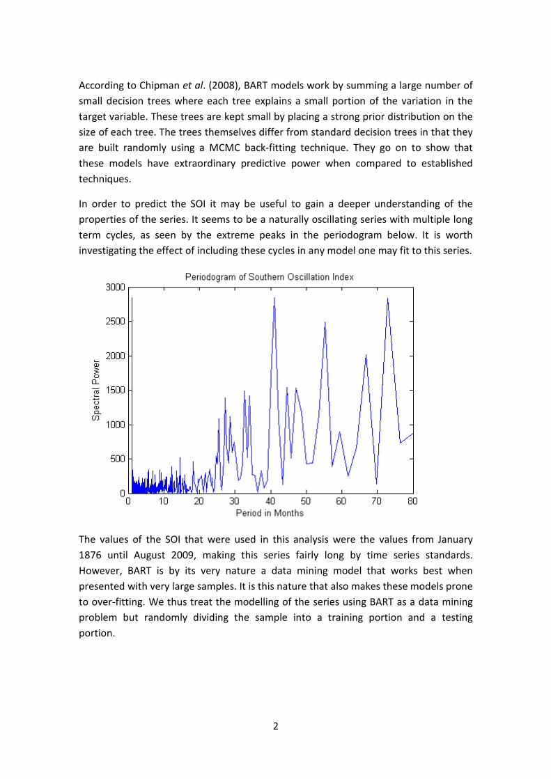
2

According to Chipman et al. (2008), BART models work by summing a large number of

small decision trees where each tree explains a small portion of the variation in the

target variable. These trees are kept small by placing a strong prior distribution on the

size of each tree. The trees themselves differ from standard decision trees in that they

are built randomly using a MCMC back-fitting technique. They go on to show that

these models have extraordinary predictive power when compared to established

techniques.

In order to predict the SOI it may be useful to gain a deeper understanding of the

properties of the series. It seems to be a naturally oscillating series with multiple long

term cycles, as seen by the extreme peaks in the periodogram below. It is worth

investigating the effect of including these cycles in any model one may fit to this series.

The values of the SOI that were used in this analysis were the values from January

1876 until August 2009, making this series fairly long by time series standards.

However, BART is by its very nature a data mining model that works best when

presented with very large samples. It is this nature that also makes these models prone

to over-fitting. We thus treat the modelling of the series using BART as a data mining

problem but randomly dividing the sample into a training portion and a testing

portion.

3

Regression Approach to Predicting October's SOI Value

Calculation of Model Accuracy

Various measures of model accuracy were calculated by comparing the predictions

with the observed values for all past Octobers, but distinguishing between those

values that were used to fit the model (sample values) and those values that were kept

aside (out-of-sample values). Three of these are reported here for every model: the

correlation coefficient (CORR), the mean absolute error (MAE) and the root mean

square error (RMSE).

It is important to note that BART models are random models, in that they produce

different results every time they are fitted. Also, the allocation of observations to the

sample versus out-of-sample is random. Thus, all results and measures reported are an

average taken over ten fits, or runs, of the model.

Using all available variables

If we build a model to predict October's value using the twelve months prior as well

the as 41st and 73rd months prior to each October we notice the presence of over-

fitting, that is to say that the out-of-sample predictions are significantly weaker than

the sample predictions.

The model mentioned above with 14 explanatory variables produces the following

mean fit statistics:

Sample CORR MAE RMSE

Training 0.92 3.23 4.04

Testing 0.72 4.89 6.18

Note that for all models in this section a random 80% of the observations are used to

train the model and the remaining 20% are used for testing.

Variable Selection

One of the reasons BART models over-fit is because too many trees are used, but that

is not the case here, as we have reduced the number of trees to just twenty. In fact,

the number of trees used does not seem to have much impact on the results at all. The

results are only slightly weaker when say ten or forty trees are used.

The reason for overfitting here seems to be that too many variables are included in the

model. We need to perform some form of variable selection, but we need to bear in

mind that we are working with a heavily non-linear model and that most standard

variable selection techniques are not appropriate. Thankfully, BART has its own,

unique, method of variable selection.

4

It works by reducing the number of trees to the point where the model has to be

selective about which variables to use in each branch. The model is then forced to seek

out those variables that are most useful in predicting the target variable. Counting the

number of times each variable is used in the model produces a measure of the relative

importance of each variable.

Applying this technique to our model produces the following relative variable

importance (1 = medium relative importance):

Variable Sep Aug Jul Jun May Apr Mar

Importance 3.04 1.21 1.68 1.35 1.00 0.60 0.49

Variable Feb Jan Dec-1 Nov-1 Oct-1 -41 -73

Importance 0.67 0.42 0.96 0.58 0.44 0.93 0.62

Reduced Model

Based on this we thus reduce our choice of variables to only the five months prior to

each October. This reduces the overfitting problem and gives results as follows:

Sample CORR MAE RMSE

Training 0.90 3.45 4.33

Testing 0.81 4.89 5.90

Note that these results can be improved by fitting the model multiple times and

selecting the best model.

There is, however, one glaring problem with this model: we only gain one month by

using it. We must have September's value in order to predict October's value.

Excluding September

We can gain another month by excluding September for the previous model. This

model is slightly weaker but is, nevertheless, the best model we can produce under

these constraints for the purpose of predicting the October value. Its fit statistics are

as follows:

Sample CORR MAE RMSE

Training 0.82 4.49 5.60

Testing 0.66 5.65 7.16

Predictions from further back in time

Making predictions using only higher lags is very difficult. We have already seen that

there is some relationship with the previous December as well as May of three years

5

prior but we were unable to find additional useful variables. Thus, we can, at best,

achieve results as follows:

Sample CORR MAE RMSE

Training 0.49 7.10 8.58

Testing 0.22 7.80 9.40

It is possible to achieve better predictions for October by not focusing on October

itself. This is especially true in the first half of each year.

Autoregressive Time Series Approach

In this section we consider every month equal and try to make predictions for the

months ahead, completely ignorant of the current date. This is closer to the classic

univariate time series approach.

When we use this approach we have twelve times as many observations and so over-

fitting is less of a concern (but still worth baring in mind). Here we increase the number

of trees in each model to 40. We also keep aside a random third of the observations

for testing (as opposed to a fifth).

Again, we need to determine the current variables to include in the model. In time

series analysis, one method that is often used is the inspection of the correlograms. If

we look at the correlograms below and we restrict ourselves to autoregressive models

then it is clear that an AR(5) model is appropriate.

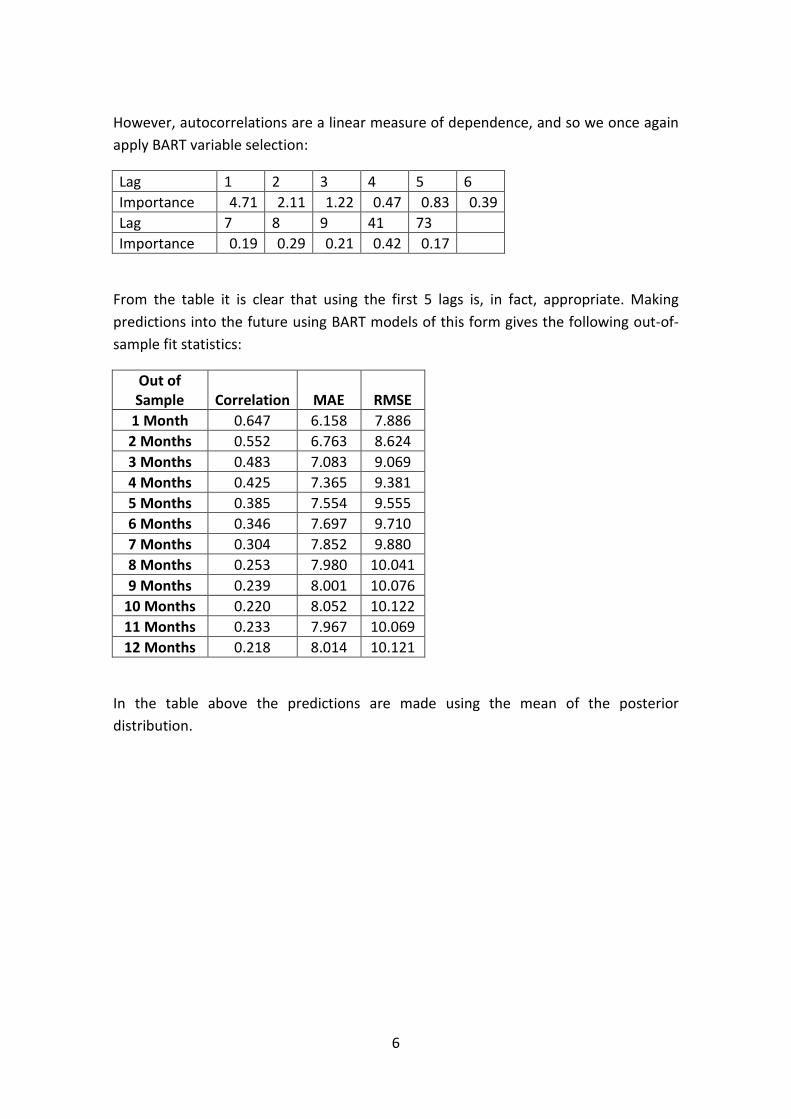
6

However, autocorrelations are a linear measure of dependence, and so we once again

apply BART variable selection:

Lag 1 2 3 4 5 6

Importance 4.71 2.11 1.22 0.47 0.83 0.39

Lag 7 8 9 41 73

Importance 0.19 0.29 0.21 0.42 0.17

From the table it is clear that using the first 5 lags is, in fact, appropriate. Making

predictions into the future using BART models of this form gives the following out-of-

sample fit statistics:

Out of

Sample Correlation MAE RMSE

1 Month 0.647 6.158 7.886

2 Months 0.552 6.763 8.624

3 Months 0.483 7.083 9.069

4 Months 0.425 7.365 9.381

5 Months 0.385 7.554 9.555

6 Months 0.346 7.697 9.710

7 Months 0.304 7.852 9.880

8 Months 0.253 7.980 10.041

9 Months 0.239 8.001 10.076

10 Months 0.220 8.052 10.122

11 Months 0.233 7.967 10.069

12 Months 0.218 8.014 10.121

In the table above the predictions are made using the mean of the posterior

distribution.

7

If we use the median of the predictive posterior instead then we get worse results:

Out of

Sample Correlation MAE RMSE

1 Month 0.638 6.238 7.978

2 Months 0.542 6.849 8.703

3 Months 0.477 7.130 9.114

4 Months 0.420 7.420 9.417

5 Months 0.374 7.651 9.633

6 Months 0.325 7.779 9.825

7 Months 0.281 7.918 9.975

8 Months 0.243 8.024 10.094

9 Months 0.207 8.110 10.193

10 Months 0.203 8.084 10.171

11 Months 0.198 8.093 10.197

12 Months 0.193 8.093 10.202

Making predictions into the future with BART models is a great deal more difficult than

it is with standard time series models as BART models do not currently allow for

situations where the output is to be fed back through the model as input.

If we are merely interested in a point estimate (as above) then we can take the mean

prediction as fact and re-fit the model with this value added onto the end of the series.

This produces a prediction for two months ahead of the current month, which can, in

turn, be added onto the series, etc.

If we require predictive intervals then the above process must be repeated many times

using a random value from the predictive posterior distribution instead of the mean or

median prediction. This process requires a distributed computing environment to

avoid excessive run times on current generation computing hardware.

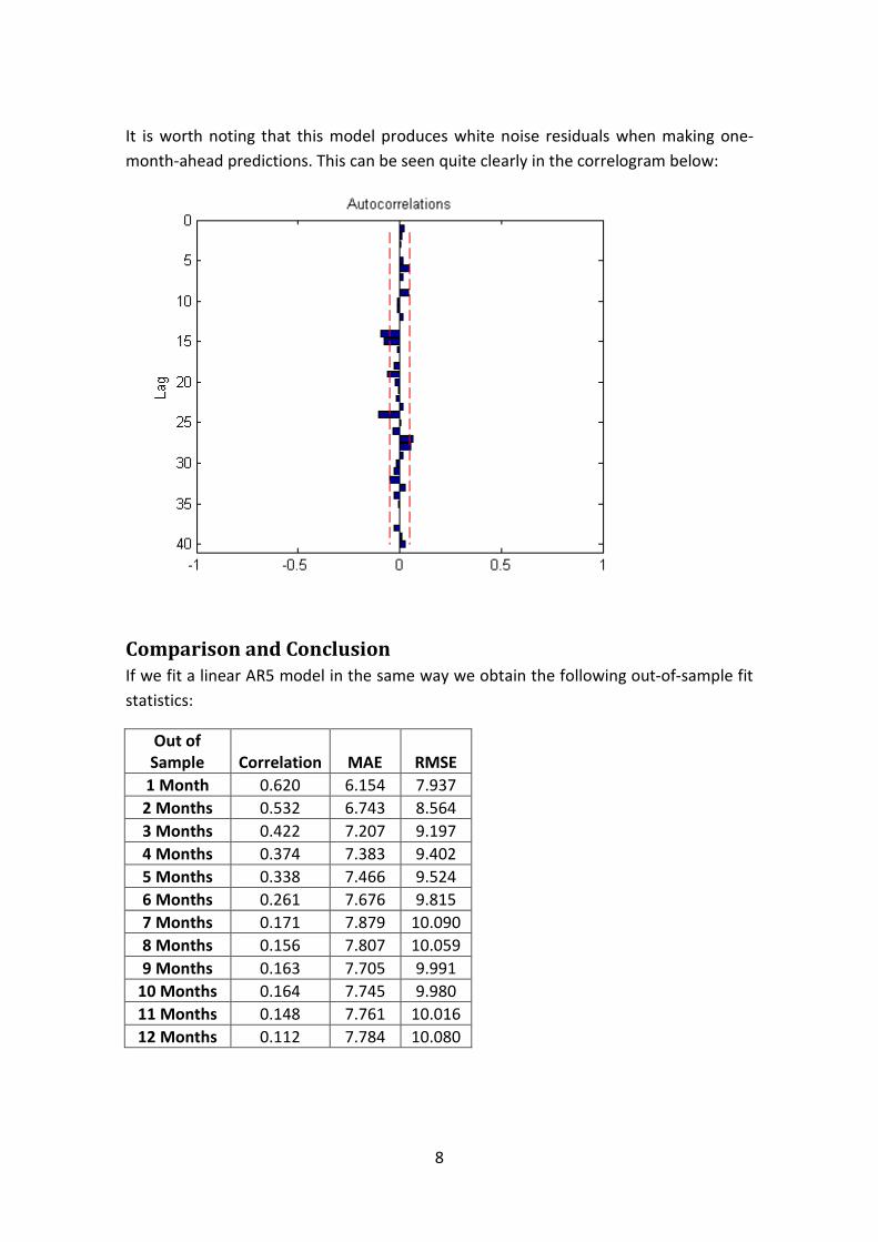
8

It is worth noting that this model produces white noise residuals when making one-

month-ahead predictions. This can be seen quite clearly in the correlogram below:

Comparison and Conclusion

If we fit a linear AR5 model in the same way we obtain the following out-of-sample fit

statistics:

Out of

Sample Correlation MAE RMSE

1 Month 0.620 6.154 7.937

2 Months 0.532 6.743 8.564

3 Months 0.422 7.207 9.197

4 Months 0.374 7.383 9.402

5 Months 0.338 7.466 9.524

6 Months 0.261 7.676 9.815

7 Months 0.171 7.879 10.090

8 Months 0.156 7.807 10.059

9 Months 0.163 7.705 9.991

10 Months 0.164 7.745 9.980

11 Months 0.148 7.761 10.016

12 Months 0.112 7.784 10.080

9

This is worse than the BART model by some way. However, if we look at the BART

predictions for the coming months we encounter a problem:

Sep 09 Oct 09 Nov 09 Dec 09 Jan 10 Feb 10

-1.97 0.40 0.77 0.09 1.15 0.71

Mar 10 Apr 10 May 10 Jun 10 Jul 10 Aug 10

0.76 0.66 0.61 0.75 0.73 0.67

It appears as though the model gradually tends towards a flat model with the variance

fading after 5 months. This may produce a relatively good fit in statistical terms but it is

of little value to the researcher wishing to know what future values of the series are

likely to be.

We obtain similar (but worse) results from the AR(5) model:

Sep 09 Oct 09 Nov 09 Dec 09 Jan 10 Feb 10

0.27 0.55 0.06 0.04 0.15 0.10

Mar 10 Apr 10 May 10 Jun 10 Jul 10 Aug 10

0.09 0.07 0.05 0.04 0.03 0.02

In conclusion, the SOI remains a very difficult time series to predict, in spite of the

power of BART models.

References

Chipman, H.A., George, E.I. and McCulloch, R.E.: 2008, Bart: Bayesian additive

regression trees. http://arxiv.org/abs/0806.3286

Chu, P.S., Katz, R.W.: 1985, Modelling and forecasting the southern oscillation: A time-

domain approach, Monthly Weather Review 113(11),pp.1876-1888.

De Waal, D.J.: 2009, Predicting losses due to spillage at the Gariep hydro-power plant.

Report to ESKOM, Feb 2009.

Giordano, F., Rocca, M.L., Perna, C.: 2007, Forecasting nonlinear time series with

neural network sieve bootstrap, Computational Statistics & Data Analysis 51,pp.3871-

3884.

Southern Oscillation Index: 2009, National Climate Centre, Australian Bureau of

Meteorology. ftp://ftp.bom.gov.au/anon/home/ncc/www/sco/soi/soiplaintext.html

Biased reduced estimators in joint tail

modelling

Beirlant J.a, Dierckx G.a,b, Guillou A.c

a Department of Mathematics and Leuven Statistics Research Centre, Katholieke Universiteit Leuven

bDepartment of Mathematics and statistics, Hogeschool-Universiteit Brussel

cIRMA, Departement de Mathematique, Universite de Strasbourg, France

October 1, 2009

Abstract

In this article we study the bias properties of the estimators based onthe first order model presented by Ledford and Tawn (1997). Theseauthors introduce the coefficient of tail dependence η, giving infor-mation about the dependence of the extreme values of two variables.We propose a bias reduced estimator for this coefficient and show itsproperties via simulations and real life examples. Further on, a biasreduced estimator for small tail probabilities follows immediately.

Keywords: Extreme value theory, bivariate slowly varying function, biasreduction

1 Joint tail modelling

Let (Z1, Z2) be a bivariate stochastic random variable with marginal distribu-tions which have already been studied. Then, without loss of generality, wecan assume that Z1 and Z2 have Frechet margins. Indeed, for bivariate (X1,X2) with general margins, the data can be transformed to Frechet marginals

using the empirical distribution functions FX1(x) and FX2

(x).

Z1 = −1/ log FX1(X1)

Z2 = −1/ log FX2(X2)

1

Then the dependence structure between the Frechet margins (Z1, Z2) can bestudied using the model of Ledford and Tawn (1997) as introduced inSection 9.5.3 in Beirlant et al. (2005).

P (Z1 > z1, Z2 > z2) = z−c11 z−c2

2 L(z1, z2), with c1 + c2 =1

η. (1)

The parameter η is called the coefficient of tail dependence whereas thefunction L is a bivariate slowly varying function. This means that thereexists a function g such that

limt→∞

L(tz1, tz2)

L(t, t)= g(z1, z2). (2)

We will assume that the function g is homogenous of order 0. This meansby definition that g(tz1, tz2) = g(z1, z2). It implies that there exists a functiong∗, such that

g(z1, z2) = g∗(z1/(z1 + z2)), (3)

In other words the function g does not change on a radius.

In Section 2 the model (1) is extended introducing a second order term. Someexamples are given to shown that this extended model is quite natural. Thissecond order model will be used in order to find bias reduced estimatorsof the parameter models and of small probabilities in Section 3. Then inSection 4, the newly introduced estimators are studied through a simulationstudy. Finally some real life examples are given in Section 5.

2 Second order model

2.1 Second order condition on LTo study how fast the limit in (2) is attained, we need a proper second or-der condition in the bivariate case. Therefore we try to extend well-knownconditions from the univariate case. Remark indeed that the bivariate slowlyvarying functions are an extension of univariate slowly varying functions ℓ.Indeed the univariate homogenous functions of order 0, are the functions gsuch that g(tz) = g(z), being the constant functions. And from the definition

limt→∞

ℓ(tz)ℓ(t)

= g(x) = a, it follows that this constant must be g(1)=1, leading

2

indeed to the definition of univariate slowly varying functions.

In order to study bias properties in the univariate case, second order condi-tions are imposed on the univariate slowly varying function. One of theseconditions is the assumption Rℓ(b, ρ), assuming that there exists ρ < 0 andb(t) → 0 as t → ∞, such that for all z > 1

ℓ(tz)

ℓ(t)∼ 1 + b(t)

zρ − 1

ρas t → ∞. (4)

A more specific condition, is the Hall condition, where

ℓ(t) ∼ C (1 + Dtρ) as t → ∞. (5)

An extension of this Hall condition to the bivariate case could be made byreplacing the constants in the univariate Hall condition again by homogenousfunctions of order 0. This leads to the following bivariate Hall condition

L(z1, z2) ∼ g1(z1, z2) (1 + g2(z1, z2)zρ1

1 zρ2

2 ) as z1, z2 → ∞. (6)

We will denote ρ1+ρ2 by ρ. Remark the analogy with model (2.2) in Ledfordand Tawn (1997).

2.2 Examples

Remark that assumption (6) holds for a lot of well-known multivariate ex-amples. Below we assume Frechet margins.

2.2.1 Morgenstern

P(Z1 6 z1, Z2 6 z2) = F (z1)F (z2)[1 + αF (z1)F (z2)

]

P(Z1 > z1, Z2 > z2) = 1 − F (z1) − F (z2) + P (Z1 6 z1, Z2 6 z2)

= 1 − e−1/z1 − e−1/z2 + e−1/z1e−1/z2

[1 + α

(1 − e−1/z1

) (1 − e−1/z2

)]

∼ 1

z1z2

[1 + α − 1 + 3α

2

(√z2

z1

+

√z1

z2

)1

√z1z2

]

3

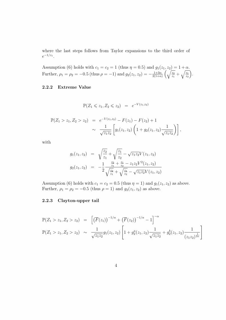
where the last steps follows from Taylor expansions to the third order ofe−1/z1 .

Assumption (6) holds with c1 = c2 = 1 (thus η = 0.5) and g1(z1, z2) = 1 + α.

Further, ρ1 = ρ2 = −0.5 (thus ρ = −1) and g2(z1, z2) = − 1+3α2(1+α)

(√z2

z1

+√

z1

z2

).

2.2.2 Extreme Value

P(Z1 6 z1, Z2 6 z2) = e−V (z1,z2)

P(Z1 > z1, Z2 > z2) = e−V (z1,z2) − F (z1) − F (z2) + 1

∼ 1√

z1z2

[g1(z1, z2)

(1 + g2(z1, z2)

1√

z1z2

)],

with

g1(z1, z2) =

√z2

z1

+

√z1

z2

−√z1z2V (z1, z2)

g2(z1, z2) = −1

2

z2

z1

+ z1

z2

− z1z2V2(z1, z2)√

z2

z1

+√

z1

z2

−√z1z2V (z1, z2)

Assumption (6) holds with c1 = c2 = 0.5 (thus η = 1) and g1(z1, z2) as above.Further, ρ1 = ρ2 = −0.5 (thus ρ = 1) and g2(z1, z2) as above.

2.2.3 Clayton-upper tail

P(Z1 > z1, Z2 > z2) =[(

F (z1))−1/α

+(F (z2)

)−1/α − 1

]−α

P(Z1 > z1, Z2 > z2) ∼ 1√

z1z2

g1(z1, z2)

[1 + ga

2(z1, z2)1

√z1z2

+ gb2(z1, z2)

1

(z1z2)1

2α

]

4

with

g1(z1, z2) =

[(z2

z1

)−

1

2α

+

(z1

z2

)−

1

2α

]−α

ga2(z1, z2) = −1

2

(z2

z1

)−

1

2α+ 1

2

+(

z1

z2

)−

1

2α+ 1

2

(z2

z1

)−

1

2α

+(

z1

z2

)−

1

2α

gb2(z1, z2) =

α(

z2

z1

)−

1

2α

+(

z1

z2

)−

1

2α

Assumption (6) holds with c1 = c2 = 0.5 and g1(z1, z2) as above. Further,

if α < 1 , ρ1 = ρ2 = −0.5 g2(z1, z2) = ga2(z1, z2)

if α = 1 , ρ1 = ρ2 = −0.5 g2(z1, z2) = ga2(z1, z2) + gb

2(z1, z2)

if α > 1 , ρ1 = ρ2 =1

2αg2(z1, z2) = gb

2(z1, z2)

Note that for α > 1, the second order term in (6) disappears slowly. This isa case where one might expect a significant improvement of the estimationwhen the second order term is added.

2.2.4 Bivariate normal

Due to the analogy with model (2.2) in Ledford and Tawn, we can use theirresults to see that c1 = c2 = 1

1+ρand ρ1 = ρ2 = 0. Also here the second order

term might result in improved estimators.

2.3 Model of Ledford and Tawn revisited, using second

order condition

We study the following transformation of (Z1, Z2), based on a treshold tand a parameter w. Consider Y given by the min(Z1/t, Z2w/[t(1 − w)])conditioned on the fact that min(Z1, Z2w/(1 − w)) > t. The parameterw can be chosen freely, while t can be chosen as the k + 1th largest orderstatistic of min(Z1, Z2w/(1−w)), as is often done in extreme value statistics.

5

It follows from (1) combined with (6) that

P(Y > z) =P(Z1 > zt, Z2 > zt(1 − w)/w)

P(Z1 > t, Z2 > t(1 − w)/w), t > 1

= z−(c1+c2)L(tz, tz(1 − w)/w)

L(t, t(1 − w)/w)

= z−1/η 1 + g2

(1, 1−w

w

)(tz)ρ1+ρ2

(1−w

w

)ρ2

1 + g2

(1, 1−w

w

)tρ1+ρ2

(1−w

w

)ρ2.

In the last step the homogeneity of the functions g1 and g2 is used.We can reparametrize this distribution as follows.

P(Y > z) ∼ z−1/η (1 + δ − δzρ)−1/η , t → ∞ (7)

with δ := ηg2

(1, 1−w

w

) (1−w

w

)ρ2 tρ1+ρ2 .

This model provides us with bias reduced estimators for η as is shown inSection 3. Moreover, the model inference can be linked to tail probabilitiesconcerning Z1 and Z2. Indeed, the probability P(Z1 > z1, Z2 > z2) can berewritten as

P(Z1 > tz, Z2 > tz 1−w

w

)

P(Z1 > t, Z2 > t1−w

w

) P

(Z1 > t, Z2 > t

1 − w

w

)(8)

= P(Y > z)P

(Z1 > t, Z2 > t

1 − w

w

), (9)

with tz = z1 and w = z1/(z1 + z2) and t chosen, as before, as the k + 1th

largest order statistic of min(Z1, Z2w/(1 − w)) .

3 Biased reduced estimators

First, we recall in short some first order biased estimators in Section 3.1.Then, we turn to estimators with reduced bias in Sections 3.2 and 3.3 basedon the second order model introduced in Section 2.

6

3.1 Biased estimation

Based on the first order terms in model (1), it immediately follows that

P(min(Z1, Z2) > r) = P(Z1 > r, Z2 > r) = r−1/ηℓ(r),

with ℓ(r) slowly varying. In other words, the variable min(Z1, Z2) is Pareto-type distributed. Therefore, the Hill estimator performed on this variableprovides an estimator of the parameter η. It should be remarked that theHill estimator is based on the k +1 largest data of min(Z1, Z2). Therefor theestimator will be denoted by ηH,k.

A first order estimator for the small tail probabilities can be found from (9).Now only P(Y > z) is estimated by solving the Weismann estimator for largequantiles of Y for small probabilities. This estimator will be denoted by pH,k.Now k refers to the treshold used for min(Z1, Z2w/(1 − w)) in Section 2.3.

3.2 Bias reduced estimation of model parameters

Based on the tail probability in (7), maximum likelihood estimators can bedetermined.Indeed, the loglikelihood of the model in (7) is given by

log L = − log η − (1/η + 1) log z − (1/η + 1) log(1 + δ − δzρ) + log(1 + δ − δzρ − δρzρ)

with partial derivatives

δ log L

δη= −1

η+

1

η2log z +

1

η2log(1 + δ − δzρ)

δ log L

δδ= − (1/η + 1)

1 − zρ

1 + δ − δzρ+

1 − zρ − ρzρ

1 + δ − δzρ − δρzρ

δ log L

δρ= (1/η + 1)

δzρ log z

1 + δ − δzρ− δzρ (1 + (1 + ρ) log z)

1 + δ − δzρ − δρzρ

In the estimation procedure however we have taken ρ equal to the canonicalvalue -1. It is known in extreme value theory that a misspecification of theparameter ρ might not affect the estimation of the parameter of main interestthat much, in this case η. We also studied the results when ρ was estimatedusing the method suggested by Fraga Alves et al. (2003). Indeed, the resultswere not much different. The resulting maximum likelihood estimator, with

7

ρ taken equal to -1, will be denoted by ηB,k. Again, k in the notation stressesthe fact that the estimator depends on the treshold used for min(Z1, Z2w/(1−w)) in Section 2.3.

3.3 Bias reduced estimation of small probabilities

Bivariate tail probabilities can now be calculated using expression (9) Theprobability P(Z1 > z1, Z2 > z2) can then be estimated as follows. P(Y >z) can be estimated by plugging in the parameter estimates in (7) andP

(Z1 > t, Z2 > t1−w

w

)can be estimated using the empirical distribution func-

tion. The resulting estimator will be denoted by pB,k.

4 Simulation results

In this section, we illustrate the finite sample properties of the previous es-timators through simulation. First, we simulated from a Morgenstern withFrechet marginals and α = 0.6. Remark that the true values η = 0.5, ρ = −1.The effect of the choice of w is examined by choosing different values. Thecorresponding tail probabilities are estimated as well.Next, we simulated from a normal copula with Frechet marginals and ρ =−0.5. w is chosen 0.5.Finally, we also show how the procedure works when general margins aregiven. We simulate from bivariate normal data (with normal marginals, in-stead of Frechet marginals). Again ρ is -0.5 in the simulation.

For each setting, 10 data sets of size n = 500 are simulated.

4.1 Morgenstern α=0.6

For the estimation of η, the parameter w can be chosen freely. First it istaken as w = 0.5. In Figure 1 the estimators ηH and the biased reducedestimator ηB are compared.Figure 1 clearly shows that ηB has better bias properties than ηH . Moreover,the choice of k seems to be less crucial for ηB.The same conclusion can be made when estimating the probability P(Z1 >20, Z2 > 20). The true value of the probability is 0.0036699. In this estima-tion in Figure 2 the value w = 0.5 is natural.

8

(a) (b)

Time

etah

[, 1]

0 100 200 300 400 500

0.0

0.2

0.4

0.6

0.8

1.0

Time

etaa

[, 1]

0 100 200 300 400 500

0.0

0.2

0.4

0.6

0.8

1.0

Figure 1: Estimators for η (a) (k, ηH,k); (b) ηB. (w=0.5)

(a) (b)

Time

prob

h[, 1

]

0 100 200 300 400 500

0.00

00.

005

0.01

00.

015

0.02

0

Time

prob

a[, 1

]

0 100 200 300 400 500

0.00

00.

005

0.01

00.

015

0.02

0

Figure 2: Estimators for P(Z1 > 20, Z2 > 20) (a) (k, pH,k); (b) pB.

The above conclusions do not heavily depend on the choice w = 0.5 as isillustrated in Figure 3 and Figure 4 for w = 15/35 = 0.42857 resp. w =8/28 = 0.285

(a) (b)

Time

etah

[, 1]

0 200 400 600 800 1000

0.0

0.2

0.4

0.6

0.8

1.0

Time

etaa

[, 1]

0 200 400 600 800 1000

0.0

0.2

0.4

0.6

0.8

1.0

Figure 3: Estimators for η (a) (k, ηH,k); (b)(k, ηB,k). (w=15/35)

The choices of w = 15/35 and w = 8/28 are also natural choice to estimatedsome probabilities. The probability P(Z1 > 15, Z2 > 20) is estimated inFigure 5. The true value of this probability is 0.0048. The probability

9

(a) (b)

Time

etah

[, 1]

0 100 200 300 400 500

0.0

0.2

0.4

0.6

0.8

1.0

Time

etaa

[, 1]

0 100 200 300 400 500

0.0

0.2

0.4

0.6

0.8

1.0

Figure 4: Estimators for η (a) (k, ηH,k); (b)(k, ηB,k). (w = 8/28

P(Z1 > 8, Z2 > 20) is estimated in Figure 6. Now , the true value of thisprobability is 0.0086.

(a) (b)

Time

prob

h[, 1

]

0 200 400 600 800 1000

0.00

00.

005

0.01

00.

015

0.02

0

Time

prob

a[, 1

]

0 200 400 600 800 1000

0.00

00.

005

0.01

00.

015

0.02

0

Figure 5: Estimators for P(Z1 > 15, Z2 > 20) (a) (k, pH,k); (b) (k, pB,k) .

(a) (b)

Time

prob

h[, 1

]

0 100 200 300 400 500

0.00

00.

005

0.01

00.

015

0.02

0

Time

prob

a[, 1

]

0 100 200 300 400 500

0.00

00.

005

0.01

00.

015

0.02

0

Figure 6: Estimators for P(Z1 > 8, Z2 > 20) (a) (k, pH,k); (b) (k, pB,k).

10

4.2 Bivariate normal ρ=-0.5, with Frechet marginals

The true value of η equals 0.25. The parameter can be chosen freely and istaken w = 0.5 in the estimation of η in Figure 11.

(a) (b)

Time

etah

[, 1]

0 100 200 300 400 500

0.0

0.1

0.2

0.3

0.4

0.5

Time

etaa

[, 1]

0 100 200 300 400 500

0.0

0.1

0.2

0.3

0.4

0.5

Figure 7: Estimators for η (a) (k, ηH,k); (b)(k, ηB,k).

The true value of the probability P(Z1 > 5, Z2 > 5) (natural choice of w =0.5) is 0.00601.

(a) (b)

Time

prob

h[, 1

]

0 100 200 300 400 500

0.00

00.

005

0.01

00.

015

0.02

0

Time

prob

a[, 1

]

0 100 200 300 400 500

0.00

00.

005

0.01

00.

015

0.02

0

Figure 8: Estimators for P(Z1 > 5, Z2 > 5) (a) (k, pH,k); (b) (k, pB,k).

4.3 Bivariate normal ρ = −0.5, with normal marginals

First the bivariate normal data are transformed into frechet marginals :

Z1 = −1/ log FX1(X1)

Z2 = −1/ log FX2(X2).

Then η can be estimated as before based on this new sample for (Z1, Z2).The probability P(X1 > x1, X2 > x2) equals

P

(Z1 > −1/ log FX1

(x1), Z2 > −1/ log FX2(x2)

):= P(Z1 > z1, Z2 > z2)

11

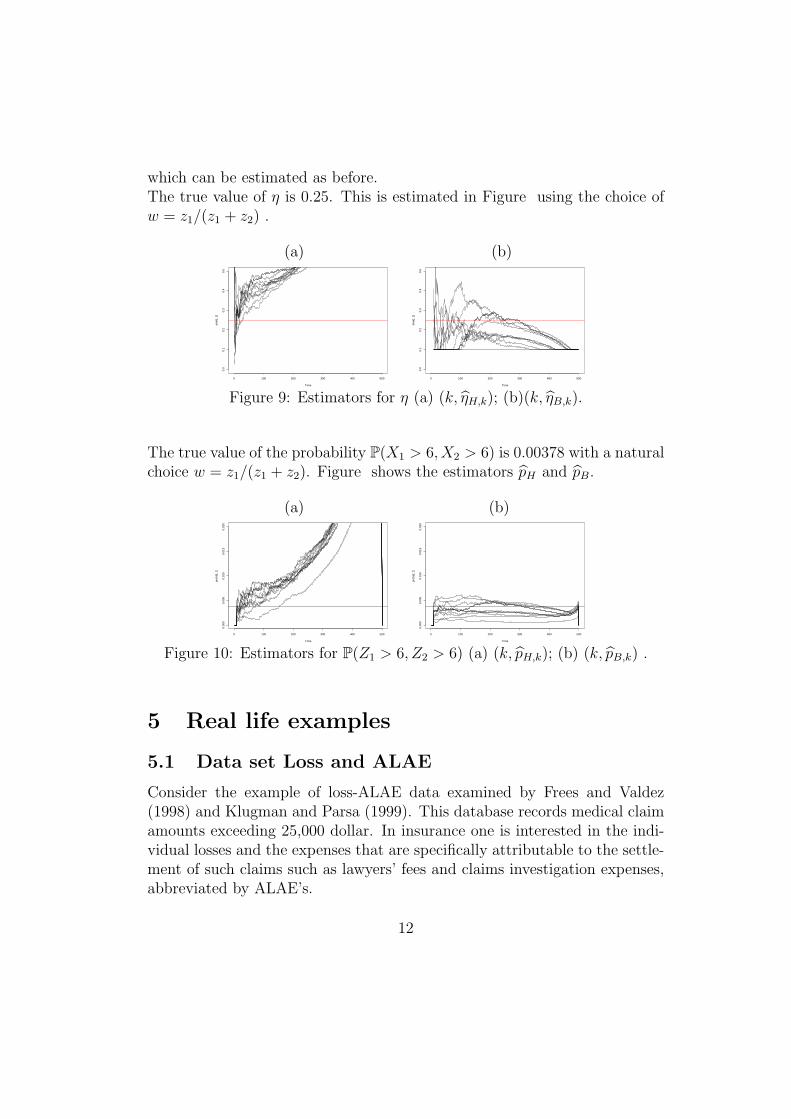
which can be estimated as before.The true value of η is 0.25. This is estimated in Figure using the choice ofw = z1/(z1 + z2) .

(a) (b)

Time

etah

[, 1]

0 100 200 300 400 500

0.0

0.1

0.2

0.3

0.4

0.5

Time

etaa

[, 1]

0 100 200 300 400 500

0.0

0.1

0.2

0.3

0.4

0.5

Figure 9: Estimators for η (a) (k, ηH,k); (b)(k, ηB,k).

The true value of the probability P(X1 > 6, X2 > 6) is 0.00378 with a naturalchoice w = z1/(z1 + z2). Figure shows the estimators pH and pB.

(a) (b)

Time

prob

h[, 1

]

0 100 200 300 400 500

0.00

00.

005

0.01

00.

015

0.02

0

Time

prob

a[, 1

]

0 100 200 300 400 500

0.00

00.

005

0.01

00.

015

0.02

0

Figure 10: Estimators for P(Z1 > 6, Z2 > 6) (a) (k, pH,k); (b) (k, pB,k) .

5 Real life examples

5.1 Data set Loss and ALAE

Consider the example of loss-ALAE data examined by Frees and Valdez(1998) and Klugman and Parsa (1999). This database records medical claimamounts exceeding 25,000 dollar. In insurance one is interested in the indi-vidual losses and the expenses that are specifically attributable to the settle-ment of such claims such as lawyers’ fees and claims investigation expenses,abbreviated by ALAE’s.

12

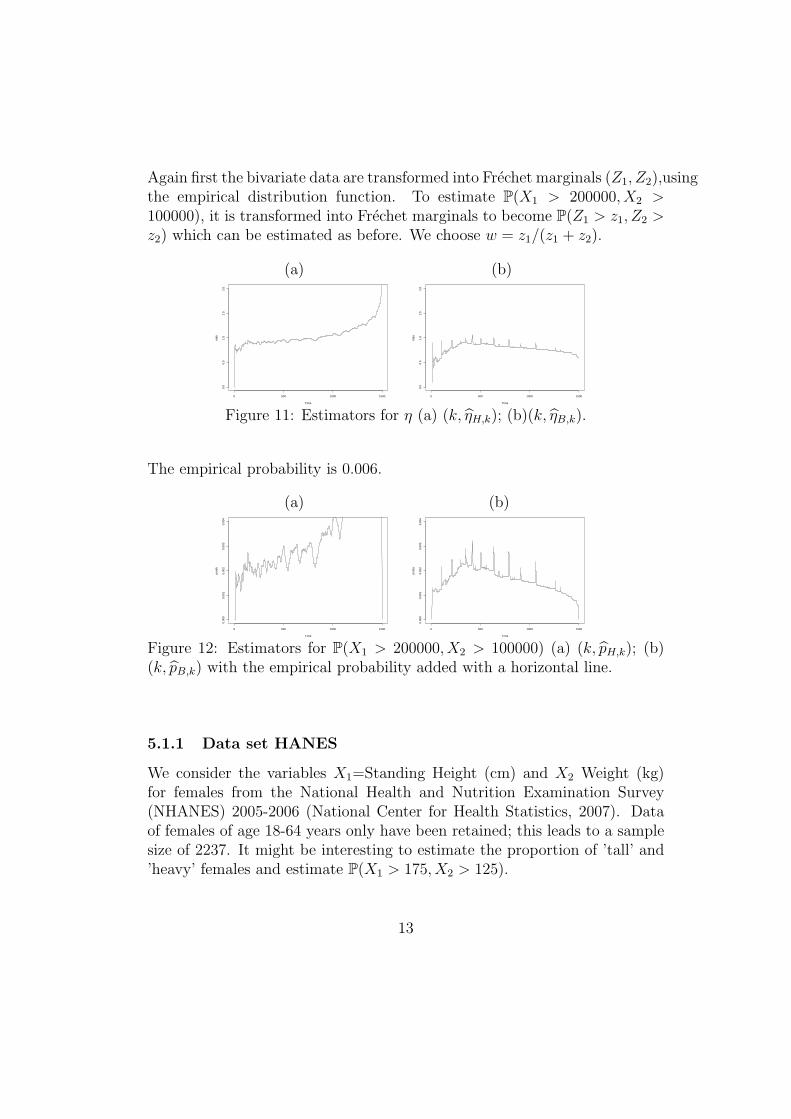
Again first the bivariate data are transformed into Frechet marginals (Z1, Z2),usingthe empirical distribution function. To estimate P(X1 > 200000, X2 >100000), it is transformed into Frechet marginals to become P(Z1 > z1, Z2 >z2) which can be estimated as before. We choose w = z1/(z1 + z2).

(a) (b)

Time

etah

0 500 1000 1500

0.0

0.5

1.0

1.5

2.0

Time

etaa

0 500 1000 1500

0.0

0.5

1.0

1.5

2.0

Figure 11: Estimators for η (a) (k, ηH,k); (b)(k, ηB,k).

The empirical probability is 0.006.

(a) (b)

Time

prob

h

0 500 1000 1500

0.00

00.

001

0.00

20.

003

0.00

4

Time

prob

a

0 500 1000 1500

0.00

00.

001

0.00

20.

003

0.00

4

Figure 12: Estimators for P(X1 > 200000, X2 > 100000) (a) (k, pH,k); (b)(k, pB,k) with the empirical probability added with a horizontal line.

5.1.1 Data set HANES

We consider the variables X1=Standing Height (cm) and X2 Weight (kg)for females from the National Health and Nutrition Examination Survey(NHANES) 2005-2006 (National Center for Health Statistics, 2007). Dataof females of age 18-64 years only have been retained; this leads to a samplesize of 2237. It might be interesting to estimate the proportion of ’tall’ and’heavy’ females and estimate P(X1 > 175, X2 > 125).

13

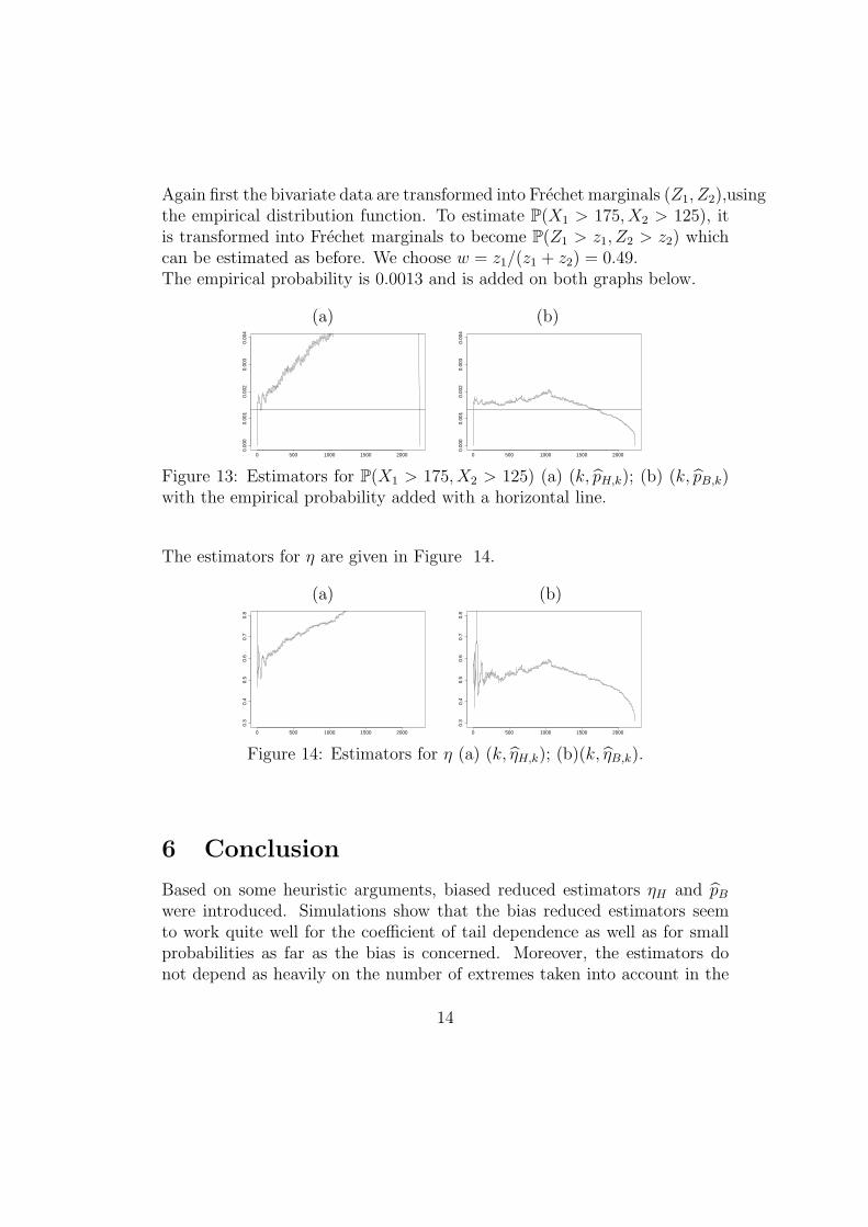
Again first the bivariate data are transformed into Frechet marginals (Z1, Z2),usingthe empirical distribution function. To estimate P(X1 > 175, X2 > 125), itis transformed into Frechet marginals to become P(Z1 > z1, Z2 > z2) whichcan be estimated as before. We choose w = z1/(z1 + z2) = 0.49.The empirical probability is 0.0013 and is added on both graphs below.

(a) (b)

0 500 1000 1500 2000

0.00

00.

001

0.00

20.

003

0.00

4

0 500 1000 1500 20000.

000

0.00

10.

002

0.00

30.

004

Figure 13: Estimators for P(X1 > 175, X2 > 125) (a) (k, pH,k); (b) (k, pB,k)with the empirical probability added with a horizontal line.

The estimators for η are given in Figure 14.

(a) (b)

0 500 1000 1500 2000

0.3

0.4

0.5

0.6

0.7

0.8

0 500 1000 1500 2000

0.3

0.4

0.5

0.6

0.7

0.8

Figure 14: Estimators for η (a) (k, ηH,k); (b)(k, ηB,k).

6 Conclusion

Based on some heuristic arguments, biased reduced estimators ηH and pB

were introduced. Simulations show that the bias reduced estimators seemto work quite well for the coefficient of tail dependence as well as for smallprobabilities as far as the bias is concerned. Moreover, the estimators donot depend as heavily on the number of extremes taken into account in the

14

estimation. Also in real life examples the bias reduced estimator seems toprovide reasonable results.

References

[1] Beirlant, J., Goegebeur, Y., Segers, J. and Teugels, J. (2005). Statisticsof Extremes: Theory and Applications. Wiley, 490p.

[2] Fraga Alves, M.I., Gomes, M.I., and de Haan, L. (2003) A new class ofsemi- parametric estimators of the second order parameter. Portugaliae

Mathematica 60, 193-214.

[3] 1998Frees98 Frees, E.W., and Valdez E.A. (1998) Understandingrelationships using copulas. North American Actuarial Journal 2, 1-15.

[4] 1999Klugman Klugman S.A., and Parsa R. (1999) Fitting bivariate lossdistributions with copulas. Insurance: Mathematics and Economics 24,139-148.

[5] Ledford, A.W. and Tawn J.A. (1997) Modelling dependence within jointtail regions. Journal of the Royal Statistical Society B, 59, 475-499.

[6] National Center for Health Statistics (2007). National Health andNutrition Examination Survey 2005-2006. Body measurementdata, http://www.cdc.gov/nchs/about/major/nhanes/nhanes2005-2006/exam0506.htm.

15

! " #

#

! # $%& ! #

' ()* $%& + ( $ (),,-**

. $%& ()* $%& / ! $%&

$%&

! # (0* ( *1

. $%& ! 2 $%&3

. 4 5 1

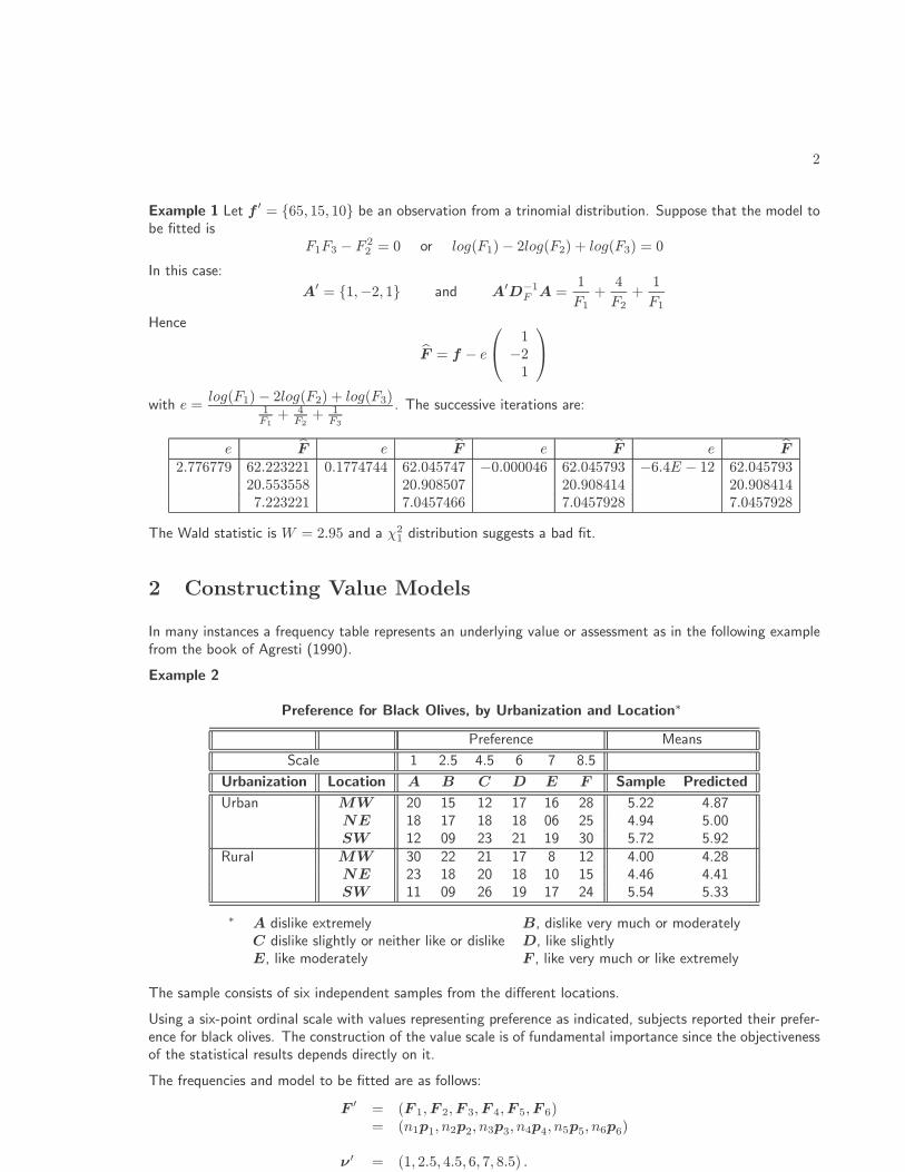
% 5

! 1

6

. 1

. 4 5

! / # ' (),,7*

!" # # $

$

) 0- 8- 9 : ;-

# $

07 )- )0 ): )9 0; -00 8;: ); ): ); ); 79 0- 8,8 -77 )0 7, 0< 0) ), <7 -:0 -,0

= <7 00 0) ): ; )0 877 80; 0< ); 07 ); )7 )- 889 88) )) 7, 09 ), ): 08 --8 -<<

# # # # # # # # #

. 2

" + " # . +

. / 5 1

(0* 1

' ' $%&3

. $%&3

! %

) 0 < 8 - -00 8;: 8,9;7: 8,98;8 8,98,: 8,98,- 8,98,9 8,8 -77 70,9-8 70,<87 70,<8) 70,<<: 70,<<: -:0 -,) "70,9-8 "70,<87 "70,<8) "70,<<: "70,<<: 877 80; "7<,<<< "7<,7<: "7<,7<: "7<,70, "7<,70, 889 88) "7099); "709<)0 "709<0- "709<08 "709<08 --8 -<< 79-,-) 79-<8, 79-<90 79-<-0 79-<-<

' (),,7* / / 5

. 4 5 8:)

. 4 / 7)09

. $%&3 / 1

! %

) 0 < 8 - -00 8,< 8,9:77 8,98-) 8,9-); 8,9-); 8,9-), 8,8 8,< 70,:8- 70,800 70,8)< 70,87; 70,87; -:0 -,) "70,:8- "70,800 "70,8)< "70,87; "70,87; 877 8<8 "7<<70; "7<09;9 "7<099: "7<099) "7<099) 889 8<8 "7<<70; "7<09;9 "7<099: "7<099) "7<099) --8 -<0 7997-: 79-<:0 79-<<8 79-<00 79-<00

. 4 5 8,-

. 4 / 009

% & '

(

. 5 ' # # 5 ! / . 7 )77

. 2 2 ! 2 # ! 2 . 2 7")77 -7 ! / . >?'%& '=&'>

. 2

') '*+*, -. &

/

$ <:908; -):9

0 0*+

"0- 8:7<0 "9):"0- 8),-; "8;00-"<7 <9)7< "0<70-"<7 <):-: ")):<7"<- <<7;; 77,<7"<- 0:8,7 7<0<-"8- -0)80 )7)<-"8- <-,<, 0;,8-@ 8097< 8)98-@ 0;)<9 977

'.

'1 <)9;7 "797 '14 0,0)< "):8 A14 )78777 779 0))<-- 00;

*1 *%

A'B '1/ );;08 <88A'B '1 ))0<:, "097A'B A1 0:)9) ";8)A'B 1/ -07-: -,9A'B 1 <0;,0 8,9A'B 1 09-9< "))7-A'B &1/ ,,9< -0,A'B &1 ,987, 08)

/

'% .

7) )<008; "0<;70")8 9))-8 "9<<)- <):<, 7;<)9"08 ),<:9 ")--0- <8;<: 00,09 )7:<7 9--0:"0, 0)0)< <:< 98,-) "<)8

& +

' <;-08 :98A :7,,7 <;0 )-88<) 777 :<898 "<;0& <;;<, ":98

+

$ CA ' (),,-* ' # ' D 0, 0,"-)

' ' (),,7* D 4 E

!"#$

% #&$'

(#$

)***

+

, ,

,

,

, , ,

-.#$/)0

1#.#$,+'(#+0'+$'+0$'-

2(#+0'+$'+0

2223!&&#,2!$&&23!&&#,23!$ !

'1#2!,2!$'- '4 5) 67 % 89

1##2!&&2!$$'- '4 5) 6789 % :9

'11

11&&1

%

% "; #%<,$

(

;#$

#% #!$,!0'!$&!

% =

#% #=!$,=!0'=!$&=!

>?# $

%

;

1'

1'

,#1' $0' (#1' '10$'

22'-'

*!

%5##,($0'#,($$

%

9% 0' (#1' '10$' 9%

9% 0' (#1' '10$' 9%

8-'@%-' *! %*!

STATISTICAL CHARACTERIZATION OF QT

PROLONGATION

Robert Schall1,2 and Arne Ring3,4

1Department of Mathematical Statistics and Actuarial Science, University of the Free

State, 9300 Bloemfontein, South Africa

2Quintiles Biostatistics, PO Box 12603, Bloemfontein 9324, South Africa

3Clinical Biostatistics, Boehringer Ingelheim Pharma, 88400 Biberach an der Riss,

Germany

4Institute for Biometry, University of Ulm, 89075 Ulm, Germany

Key Words: Bazett; ECG; Fridericia; Heart rate correction; Mixed models; QT

interval; Thorough QT study; Torsades des pointes.

1

ABSTRACT

The appropriate assessment of QT prolongation remains controversial. We suggest

that, before the relative merits of various methods can be evaluated, we must state what

we assume an assessment of QT prolongation should be about. As a general framework

for the assessment of QT prolongation we propose that an assessment of “absolute” or

“uncorrected” QT prolongation is properly carried out through a between-treatment

(active versus placebo) comparison of the marginal distributions of QT data; an as-

sessment of “heart rate corrected” QT prolongation is carried out through a between-

treatment comparison of the conditional distributions of QT data (conditional on RR

interval or heart rate). Under this general framework, conditional QT prolongation is,

in general, a function of RR interval, and we discuss three possible summary charac-

teristics for that function. We show how current procedures for the assessment of QT

prolongation relate to the general approach (that is, to between-treatment contrasts

of the marginal and conditional expectation of the QT interval), and to each other. It

transpires that only the so-called “one-step procedure” can provide a complete char-

acterization of conditional QT prolongation. We show that the “two-step procedure”

with data driven correction provides an unbiased estimate of expected conditional QT

prolongation, which may, from a clinical point of view, be a more satisfactory char-

acteristic than the conventional characteristic, QT prolongation at the reference RR

interval. We strongly suggest that two-step procedures with fixed correction be aban-

doned in the analysis of thorough QT/QTc studies: fixed correction is either redundant

(when a drug has no effect on RR average interval), or systematically biased (when a

drug does affect average RR interval).

2

1. INTRODUCTION

1.1. QT Prolongation

An undesirable property of some non-anti-arrhythmic drugs is their ability to de-

lay cardiac repolarization, an effect that can be measured as prolongation of the QT

interval on the surface electrocardiogram (ECG) (ICH 2005). A delay in cardiac re-

polarization is associated with the development of arrhythmia, in particular Torsades

de Pointes, which may be life-threatening. Thus prolongation of the QT interval is

used as a biomarker for cardiac safety. In recent years, regulatory authorities require

that every new drug undergo clinical electrographic evaluation. Typically QT data

is collected early in the drug’s development, to be followed by a so-called “thorough

QT/QTc study” in healthy subjects (ICH 2005). If a drug’s potential for QT prolon-

gation cannot be ruled out based on the results of those studies, an expanded ECG

safety evaluation during later stages of drug development must be conducted, including

clinical trials in the target population. Alternatively, the drug’s development might be

terminated. Either way, the assessment of QT prolongation is a crucial part of drug

development and in recent years has generated intensive discussion in the medical and

statistical literature.

1.2. Effect of RR Interval

Because the QT interval is associated with the RR interval (which is the inverse of

the heart rate), the potential of a drug to prolong the QT interval could be “masked”

if the drug decreases the RR interval. Conversely, a drug that does not prolong the

QT interval may appear to do so if the drug increases the RR interval. Therefore,

when a drug affects the RR interval, the drug’s effect on the QT interval must be

distinguished from changes in QT interval due to changes in RR interval (Li et al,

2004). For this reason, QT interval data is routinely “corrected” for RR interval using

various correction formulae or procedures, to obtain a value known as the QTc interval

which is hoped to be independent of RR interval, or at least less dependent of RR

interval than the QT interval itself (ICH 2005). However, as the ICH (2005) guidance

3

document states, it is not yet clear whether cardiac arrhythmia is more closely related

to an increase in the absolute (ie. uncorrected) QT interval or to an increase in QTc.

As long is this clinical question is open, both QT and QTc data have to be studied.

1.3. Current Approaches to Assessment of QT Prolongation

Historically, the analysis of QT data proceeds in two steps (Li et al, 2004): In the

first step, the QT interval data is corrected for the effect of heart rate, using one of

the following two correction procedures: either (i) “Fixed” correction where one of

a number of published correction formulae is used to calculate QTc as a function of

QT and HR; or (ii) “Off-drug data driven” correction where the slope estimate from

a regression of placebo (off-drug) QT data against heart rate is used to calculate QTc

for both active and placebo treatment data. Thereafter, in the second step, the QTc

data of active and placebo treatment are compared statistically.

More recently, Li et al (2004) and other authors have pointed out that, from a statis-

tician’s perspective, a so-called “one-step” statistical analysis of both active treatment

and placebo QT data, using mixed model analysis of covariance (where RR is fitted as

a covariate) would be preferable to the two-step approach. Nevertheless, many clinical

pharmacologists and other medical researchers seem to be comfortable with the two-

step analysis and the ICH (2005) guidance as well as most analyses of QT/QTc trials

in practice adhere to the two-step approach. The situation persists despite published

work pointing out serious shortcomings of the various two-step approaches (Dmitrienko

and Smith, 2003; Shah and Hajian, 2003; Li et al, 2004; Wang, Pan and Balch, 2008).

1.4. Outline of the Rest of the Paper

The appropriate assessment of QT prolongation evidently remains controversial.

We suggest that, before the relative merits of the various methods for assessment of

QT prolongation can be evaluated, a basis for discussion is needed. At a minimum, we

must explicitly state what we assume an assessment of QT prolongation is (or should

be) about. In Section 2, therefore, we propose a general and basic principle for the

4

assessment of QT prolongation: We suggest that an assessment of uncorrected or “ab-

solute” QT prolongation is properly carried out through a between-treatment (active

versus placebo) comparison of the marginal distributions of QT data; an assessment

of “heart rate corrected” QT prolongation is carried out through a between-treatment

comparison of the conditional distributions of QT data (conditional on RR interval).

Current procedures (analysis of central tendency and categorical analysis of QT pro-

longation (ICH 2005, Section 3.2)) emerge as special cases.

Both the relevant literature and current practice focus on the case where the con-

ditional expectation of QT data is written as a linear or log-linear function of the RR

interval. In Section 3 we adopt this approach and argue that, in general, the linear

or log-linear model should allow for unequal slopes for the regression of QT against

RR interval. Thus conditional QT prolongation is, in general, a function of RR in-

terval. We discuss three possible summary characteristics for that function, and show

how the various characteristics for assessment of both marginal and conditional QT

prolongation can be given a geometric interpretation.

In Section 4 we show how current procedures for assessment of QT prolongation

relate to the general approach (that is, to between-treatment contrasts of the marginal

and conditional expectation of the QT interval), and to each other. It transpires that, in

general, only the one-step procedure provides a complete characterization of conditional

QT prolongation. We show that the two-step procedure with data driven correction

provides an unbiased estimate of expected conditional QT prolongation, which may,

from a clinical point of view, be a more satisfactory characteristic than the conventional

characteristic, QT prolongation at the reference RR interval. The two-step procedure

with fixed correction is either redundant (when a drug has no effect on RR average

interval), or potentially biased (when a drug does affect average RR interval).

In Section 5 we sketch a procedure and statistical decision rule for assessment of

QT prolongation. When QT data is analyzed on the logarithmic scale, we propose to

formulate the statistical decision rule on the ratio scale. Section 6 is devoted to an

5

example of application, and Section 7 to the discussion.

In summary, our paper focuses on the parametric characterization of QT prolonga-

tion. We aim to answer the following question: which parameter contrast is statistical

inference about under various current QT assessment procedures (one-step procedure,

two-step procedure with data driven correction, two-step procedure with fixed cor-

rection, analysis of uncorrected data). We also make a suggestion regarding which

parameter contrast statistical inference should be about in our view. Details of the

estimation or testing of the parameter contrasts in question are not of primary interest

in the present paper.

2. MARGINAL VERSUS CONDITIONAL QT PROLONGATION

Let QT denote a QT interval measurement and RR the corresponding RR interval.

We define y = f(QT ) and x = f(RR), where f(·) is a suitable monotonic transfor-

mation. Usually, f(·) is either the identity function or the natural logarithm (Malik

et al. 2002; Ring, 2009). The bivariate random variables (yA, xA) and (yP , xP ) denote

the paired (possibly transformed) QT and RR interval measurements under active (A)

and placebo (P) treatment, respectively. Furthermore, FA and FP denote the marginal

distributions of yA and yP , FA|x and FP |x the conditional distributions of yA and yP

(conditional on a given value of x), and GA and GP the marginal distributions of xA

and xP .

We define the assessment of “uncorrected” or “absolute” QT prolongation as a

between-treatment (active versus placebo) comparison of the marginal distributions

FA and FP ; in the following, we will refer to such a comparison as an assessment

of marginal QT prolongation. Similarly, we define the assessment of “heart rate

corrected” QT prolongation as a between-treatment comparison of the conditional

distributions FA|x and FP |x; we will refer to such a comparison as an assessment of

conditional QT prolongation.

While in general an assessment of marginal and conditional QT prolongation in-

volves a comparison of marginal and conditional distributions of QT measurements,

6

in practice such a comparison will focus on specific parameters or functions of those

distributions. Below, we present two such types of characteristics.

2.1. Characteristics for Marginal QT Prolongation

An assessment of marginal QT prolongation may focus on the means E(yA) =

EFA(yA) = µA and E(yP ) = EFP

(yP ) = µP of the relevant marginal distributions FA

and FP ; in the terminology of the relevant ICH guidance (ICH 2005, Section 3.2.1) a

comparison of means constitutes an analysis of the “central tendency” of QT measure-

ments. Then the between-treatment contrast of marginal means,

γm = µA − µP (1)

can be viewed as a “moment-based” characteristic for marginal QT prolongation, to

use terminology from area of bioequivalence assessment (Schall and Luus, 1993). (The

subscript “m” in γm stands for “marginal”.)

Of course the difference in means is not the only criterion that can be used to

compare the distributions FA and FP in a clinically meaningful way. For example,

so-called “categorical” analyses (ICH 2005, Section 3.2.2) involve estimation of excess

probabilities of the form ProbFA(yA > c) and ProbFP

(yP > c), where c represents a

clinically relevant cut-off value for y, such as c = f(450ms), c = f(480ms) or c =

f(500ms). A “probability-based” characteristic for marginal QT prolongation could

then be defined as the risk ratio

ρm,d =ProbFA

(yA > d)

ProbFP(yP > d)

(2)

Alternatively, the odds ratio or risk difference involving the excess probabilities for

active and placebo treatment could be used to characterize relative risk.

2.2. Characteristics for Conditional QT Prolongation

An assessment of conditional QT prolongation may focus on the conditional means

E(yA|x) = EFA|x(yA) and E(yP |x) = EFP |x(yP ) of yA and yP . Then, a moment-based

7

characteristic for conditional QT prolongation is the between-treatment contrast of

conditional means

γc(x) = E(yA|x)− E(yP |x) (3)

which in general is a function of x. (The subscript “c” in γc(x) stands for “condi-

tional”.) We note that Equation (3) does not necessarily require a linear model for

the conditional means. In principle, E(yA|x) and E(yP |x), and consequently γ(x), can

be estimated using non-linear or nonparametric regression techniques. However, in

the following we concentrate on the case when E(yA|x) and E(yP |x) can be written as

linear functions of x.

Similarly to Equation (2), a probability-based characteristic for conditional QT

prolongation can be defined as the risk ratio

ρc,d(x) =ProbFA |x(yA > d)

ProbFP |x(yP > d)=

ProbFA(yA > d | x)

ProbFP(yP > d | x)

(4)

3. CHARACTERIZATION OF QT PROLONGATION UNDER

LINEAR/LOG-LINEAR MODEL

3.1. Linear/Log-linear Model for QT Data

In the spirit of Dmitrienko and Smith (2003), Shah and Hajian (2003) and Li et al

(2004) we postulate the following linear model for the conditional expectations E(yA|x)

and E(yP |x) as a function of x:

E(yi|x) = αi + βi · (x− xr); i = A, P (5)

Here xr = f(RRr) = f(1000), where RRr = 1000 ms is the fixed value of the so-called

“reference” RR interval corresponding to a heart rate of 60 beats/min. Note that in

Model (5) we allow, in general, for different (non-parallel) slopes βA and βP for active

and placebo treatment, respectively. When f(·) is the identity function, Model (5) is

linear; when f(·) is the logarithm, Model (5) is log-linear.

In terms of the parameters of Model (5), and of the marginal means EGA(xA) =

E(xA) = νA and EGP(xP ) = E(xP ) = νP of xA and xP , the unconditional expectations

8

of yA and yP are given by

E(yi) = µi = αi + βi · (νi − xr); i = A, P (6)

We can now express the moment-based characteristics for marginal and conditional

QT prolongation – Equations (1) and (3), respectively – in terms of the parameters of

Model (5) and of the expected values of xA and xP .

To illustrate the various characteristics for QT prolongation, in Figure 1 we present

a schematic plot of the regression lines specified in Model (5), namely of E(yA|x) and

E(yP |x). For simplicity, but without loss of generality we assume that (5) represents a

log-linear model with xr = log(1[s]) = 0.

3.2. Marginal QT prolongation

Although not necessary for the assessment of marginal QT prolongation, it will be

instructive to express γm in terms of the parameters of Model (5), using Equation (6):

γm = µA − µP = [αA + βA · (νA − xr)] − [αP + βP · (νP − xr)] (7)

Thus γm, the treatment contrast for assessment of marginal QT prolongation, can be

written as γm = E(yA|νA) − E(yP |νP ).

We note that the contrast γm can be obtained geometrically as follows: project the

points E(yA|νA) and E(yP |νP ) parallel with the x-axis (that is, using a slope of zero)

onto the y-axis; γm is then given by the difference of the projections of E(yA|νA) and

E(yP |νP ) onto the y-axis (Figure 1). Below we will show how the various characteristics

for conditional QT prolongation can also be obtained geometrically, namely as the

difference of projections of E(yA|νA) and E(yP |νP ) onto the y-axis using particular sets

of regression slopes (Table 1).

3.3. Conditional QT prolongation

Using Equation (5), we can write the between-treatment contrast of conditional

means, γc(x) in (3), as

γc(x) = E(yA|x)− E(yP |x) = αA − αP + (βA − βP ) · (x − xr) (8)

9

When, in Model (5), we are willing to assume that the slopes are equal (βA = βP),

γc(x) simplifies to γc(x) ≡ γc ≡ αA − αP , and conditional QT prolongation is charac-

terized globally (independent of RR interval) by the difference in intercepts αA − αP .

However, in general the assumption of equal slopes cannot be made so that the extent

of conditional QT prolongation, γc(x), depends on x = f(RR). For use in a statis-

tical decision rule, we might consider the following three summary characteristics for

conditional QT prolongation: (i) conditional QT prolongation γc(x) evaluated at some

reference RR interval; (ii) the expected value of conditional QT prolongation γc(x);

(iii) the maximum conditional QT prolongation γc(x) over a “reference range” of RR

interval values, that is, the maximum of γc(x) over a clinically relevant range [x0, x1]

of values of x.

(i) Conditional QT prolongation at some reference RR interval

Characteristic γc(x) evaluated at the conventional reference RR interval is given by

γc(xr) = αA − αP (9)

Characteristic (9) is commonly viewed almost as the “definition” of (conditional) QT

prolongation. However, in the case of unequal slopes under Model (5), γc(xr) charac-

terizes conditional QT prolongation only for one particular RR interval, namely for the

conventional reference RR interval RRr = 1 s, and one may suspect that RRr = 1 s

was not necessarily chosen for its clinical relevance but simply because it is a “round”

number. Therefore, regulatory authorities might consider changing the definition of

reference RR interval, for example to a value that better represents the typical RR

interval seen in the patient target population.

Geometrically, γc(xr) can be obtained as follows: project the points E(yA|νA) and

E(yP |νP ) onto the y-axis using the respective regression slopes βA and βP ; γc(xr) is

then given by the difference of these projections, namely as the difference of intercepts

αA − αP (Figure 1; Table 1).

10

(ii) Expected value of conditional QT prolongation

The expected value of γc(x), taking the expectation with respect to the distribution

GA of x = f(RR) under active treatment, is given by

EGAγc(x) = αA − αP + (βA − βP ) · (νA − xr) = γc(νA) (10)

Characteristic (10) can be interpreted as contrast γc(x) evaluated at the expected value

νA of x under active treatment.

Geometrically, γc(νA) can be obtained as follows: project both, E(yA|νA) and E(yP |νP ),

onto the y-axis using the regression slope βP for placebo; γc(νA) is then given by the

difference of the projections (Figure 1; Table 1).

(iii) Maximum conditional QT prolongation over RR reference range

If x ∈ [x0, x1] is a clinically relevant range of values of x, which we refer to as the

“reference range” of RR interval (or heart rate) values, then the maximum conditional

QT prolongation over that range is given by

γc,max = maxγc(x) | x0 ≤ x ≤ x1 = maxγ(x0), γ(x1) (11)

One could view characteristic (11) as a generalization of characteristic (9), in the

sense that instead of considering conditional QT prolongation only at one particular

value of RR interval, (maximum) conditional QT prolongation over a range of values

is considered. Thorough QT/QTc studies are usually conducted in healthy young

subjects, whose average heart rate may well be around 60 (although heart rates under

50 beats/min are often observed). However, the distribution of heart rates of a potential

target patient population is likely to be shifted to the right. By specifying [x0, x1] so

as to represent a range of heart rates from 50 to 70 beats/min, say, (11) would also

characterize potential QT prolongation at higher heart rates.

4. CONVENTIONAL PROCEDURES IN THE LIGHT OF THE GEN-

ERAL APPROACH

11

4.1. One-Step Procedure

In the one-step procedure, Model (5) is fitted simultaneously to both active and

placebo data, usually through a linear or log-linear mixed model. From the fitted

model, unbiased and efficient point and interval estimates for characteristic γc(x) in (8)

can be obtained for any x, that is, over any range of RR interval values of interest (not

only for xr, the reference RR interval). In that sense, the one-step procedure provides

a “complete” characterization of conditional QT prolongation. Furthermore, the one-

step procedure provides a sound statistical setting for testing specific hypotheses of

interest, such as the hypothesis of equal slopes βA and βP in Model (5); as we shall

see, the question of equal slopes βA and βP is highly relevant, both statistically and

clinically, to the problem of heart rate correction.

In a conventional application of the one-step procedure, statistical inference is about

the parameter contrast γc(xr) = αA − αP , which is summary characteristic (i) of

γc(x) from the general approach: Conditional QT prolongation at some reference RR

interval. As noted before, however, in the general case of unequal slopes βA 6= βB in

Model (5), γc(xr) is not necessarily the most appropriate characteristic for conditional

QT prolongation and the one-step procedure can be used to characterize conditional

QT prolongation more completely.

4.2. Two-Step Procedure with Data Driven Correction

The so-called two-step procedure proceeds as follows: In Step 1, a model of type

(5) is fitted to the placebo (or drug-free baseline) data only, namely E(yP |x) = αP +

βP · (xP −xr). From this model, an estimate βP of the slope βP is obtained. Note that

the slope estimate βP might have been obtained either as a “pooled” estimate – Model

(5) is fitted to the pooled placebo data – or as “individual” estimate – slope estimates

are obtained individually for each subject in the placebo group. The slope estimate is

then used to correct both the active and placebo data as follows:

ycA = yA − βP · (xA − xr)

12

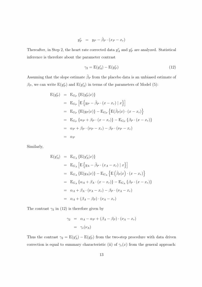
ycP = yP − βP · (xP − xr)

Thereafter, in Step 2, the heart rate corrected data ycA and yc

P are analyzed. Statistical

inference is therefore about the parameter contrast

γ2 = E(ycA) − E(yc

P ) (12)

Assuming that the slope estimate βP from the placebo data is an unbiased estimate of

βP , we can write E(ycP ) and E(yc

A) in terms of the parameters of Model (5):

E(ycP ) = EGP

E(ycP |x)

= EGP

[

E

yP − βP · (x− xr) | x]

= EGPE(yP |x) − EGP

E(βP |x) · (x − xr)

= EGPαP + βP · (x − xr) − EGP

βP · (x − xr)

= αP + βP · (νP − xr) − βP · (νP − xr)

= αP

Similarly,

E(ycA) = EGA

E(ycA|x)

= EGA

[

E

yA − βP · (xA − xr) | x]

= EGAE(yA|x) − EGA

E(

βP |x)

· (x − xr)

= EGAαA + βA · (x − xr) − EGA

βP · (x − xr)

= αA + βA · (νA − xr) − βP · (νA − xr)

= αA + (βA − βP ) · (νA − xr)

The contrast γ2 in (12) is therefore given by

γ2 = αA − αP + (βA − βP ) · (νA − xr)

= γc(νA)

Thus the contrast γ2 = E(ycA) − E(yc

P ) from the two-step procedure with data driven

correction is equal to summary characteristic (ii) of γc(x) from the general approach:

13

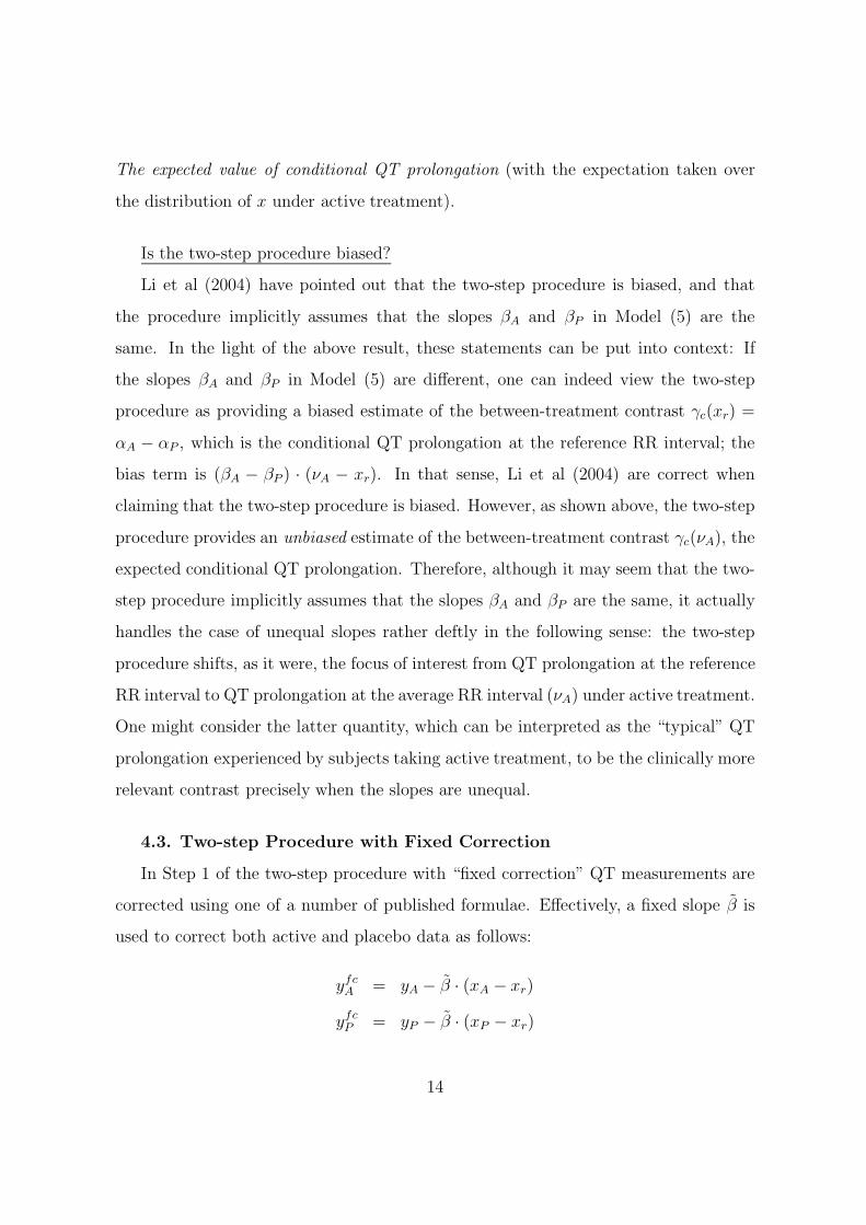
The expected value of conditional QT prolongation (with the expectation taken over

the distribution of x under active treatment).

Is the two-step procedure biased?

Li et al (2004) have pointed out that the two-step procedure is biased, and that

the procedure implicitly assumes that the slopes βA and βP in Model (5) are the

same. In the light of the above result, these statements can be put into context: If

the slopes βA and βP in Model (5) are different, one can indeed view the two-step

procedure as providing a biased estimate of the between-treatment contrast γc(xr) =

αA − αP , which is the conditional QT prolongation at the reference RR interval; the

bias term is (βA − βP ) · (νA − xr). In that sense, Li et al (2004) are correct when

claiming that the two-step procedure is biased. However, as shown above, the two-step

procedure provides an unbiased estimate of the between-treatment contrast γc(νA), the

expected conditional QT prolongation. Therefore, although it may seem that the two-

step procedure implicitly assumes that the slopes βA and βP are the same, it actually

handles the case of unequal slopes rather deftly in the following sense: the two-step

procedure shifts, as it were, the focus of interest from QT prolongation at the reference

RR interval to QT prolongation at the average RR interval (νA) under active treatment.

One might consider the latter quantity, which can be interpreted as the “typical” QT

prolongation experienced by subjects taking active treatment, to be the clinically more

relevant contrast precisely when the slopes are unequal.

4.3. Two-step Procedure with Fixed Correction

In Step 1 of the two-step procedure with “fixed correction” QT measurements are

corrected using one of a number of published formulae. Effectively, a fixed slope β is

used to correct both active and placebo data as follows:

yfcA = yA − β · (xA − xr)

yfcP = yP − β · (xP − xr)

14

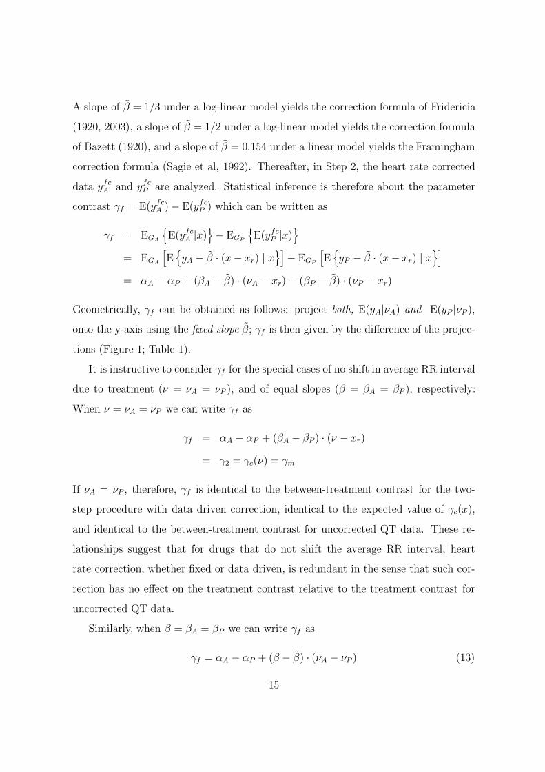
A slope of β = 1/3 under a log-linear model yields the correction formula of Fridericia

(1920, 2003), a slope of β = 1/2 under a log-linear model yields the correction formula

of Bazett (1920), and a slope of β = 0.154 under a linear model yields the Framingham

correction formula (Sagie et al, 1992). Thereafter, in Step 2, the heart rate corrected

data yfcA and yfc

P are analyzed. Statistical inference is therefore about the parameter

contrast γf = E(yfcA ) − E(yfc

P ) which can be written as

γf = EGA

E(yfcA |x)

− EGP

E(yfcP |x)

= EGA

[

E

yA − β · (x− xr) | x]

− EGP

[

E

yP − β · (x − xr) | x]

= αA − αP + (βA − β) · (νA − xr) − (βP − β) · (νP − xr)

Geometrically, γf can be obtained as follows: project both, E(yA|νA) and E(yP |νP ),

onto the y-axis using the fixed slope β; γf is then given by the difference of the projec-

tions (Figure 1; Table 1).

It is instructive to consider γf for the special cases of no shift in average RR interval

due to treatment (ν = νA = νP ), and of equal slopes (β = βA = βP ), respectively:

When ν = νA = νP we can write γf as

γf = αA − αP + (βA − βP) · (ν − xr)

= γ2 = γc(ν) = γm

If νA = νP , therefore, γf is identical to the between-treatment contrast for the two-

step procedure with data driven correction, identical to the expected value of γc(x),

and identical to the between-treatment contrast for uncorrected QT data. These re-

lationships suggest that for drugs that do not shift the average RR interval, heart

rate correction, whether fixed or data driven, is redundant in the sense that such cor-

rection has no effect on the treatment contrast relative to the treatment contrast for

uncorrected QT data.

Similarly, when β = βA = βP we can write γf as

γf = αA − αP + (β − β) · (νA − νP ) (13)

15

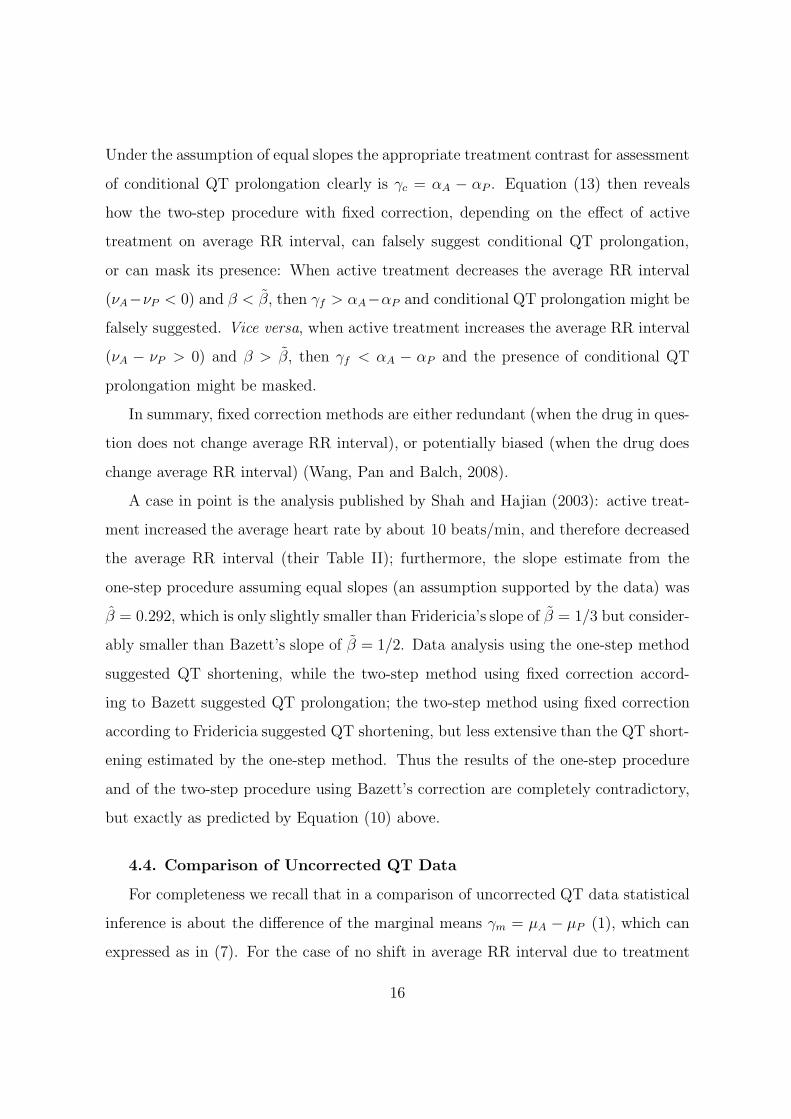
Under the assumption of equal slopes the appropriate treatment contrast for assessment

of conditional QT prolongation clearly is γc = αA − αP . Equation (13) then reveals

how the two-step procedure with fixed correction, depending on the effect of active

treatment on average RR interval, can falsely suggest conditional QT prolongation,

or can mask its presence: When active treatment decreases the average RR interval

(νA−νP < 0) and β < β, then γf > αA−αP and conditional QT prolongation might be

falsely suggested. Vice versa, when active treatment increases the average RR interval

(νA − νP > 0) and β > β, then γf < αA − αP and the presence of conditional QT

prolongation might be masked.

In summary, fixed correction methods are either redundant (when the drug in ques-

tion does not change average RR interval), or potentially biased (when the drug does

change average RR interval) (Wang, Pan and Balch, 2008).

A case in point is the analysis published by Shah and Hajian (2003): active treat-

ment increased the average heart rate by about 10 beats/min, and therefore decreased

the average RR interval (their Table II); furthermore, the slope estimate from the

one-step procedure assuming equal slopes (an assumption supported by the data) was

β = 0.292, which is only slightly smaller than Fridericia’s slope of β = 1/3 but consider-

ably smaller than Bazett’s slope of β = 1/2. Data analysis using the one-step method

suggested QT shortening, while the two-step method using fixed correction accord-

ing to Bazett suggested QT prolongation; the two-step method using fixed correction

according to Fridericia suggested QT shortening, but less extensive than the QT short-

ening estimated by the one-step method. Thus the results of the one-step procedure

and of the two-step procedure using Bazett’s correction are completely contradictory,

but exactly as predicted by Equation (10) above.

4.4. Comparison of Uncorrected QT Data

For completeness we recall that in a comparison of uncorrected QT data statistical

inference is about the difference of the marginal means γm = µA − µP (1), which can

expressed as in (7). For the case of no shift in average RR interval due to treatment

16

(ν = νA = νP ), we have already pointed out in Section 4.3 that γm = γ2 = γf = γc(ν).

Thus, when a drug does not shift the average RR interval, marginal QT prolongation

(γm) is the same as conditional QT prolongation at the average RR interval (γc(ν)).

Note, however, when βA 6= βP , an assessment of conditional QT prolongation using

characteristics γc(xr) and γc,max can still provide information different to an assessment

of marginal QT prolongation, because γc(xr) and γc,max characterize conditional QT

prolongation at RR intervals other than ν.

In the case of equal slopes, β = βA = βP , γm is given by

γm = αA − αP + β · (νA − νP ) (14)

Under the assumption of equal slopes the appropriate characteristic for assessment of

average conditional QT prolongation clearly is γc(x) ≡ γc = αA − αP . Equation (14)

then reveals why in general (νA 6= νP ) an assessment of marginal QT prolongation – sta-

tistical inference on γm – can indeed provide different information from an assessment

of conditional QT prolongation: β is always positive, and if active treatment decreases

the average RR interval (νA < νP ), then conditional QT prolongation (αA αP )

might be present in the absence of marginal QT prolongation, since β · (νA − νP ) is

negative and consequently γm might be small even when αA αP . Conversely, if

active treatment increases the average RR interval (νA > νP ), then β · (νA− νP ) is pos-

itive and therefore γm might be large (presence of marginal QT prolongation) although

there is no conditional QT prolongation (αA − αP ≈ 0).

5. PROPOSED ASSESSMENT OF QT PROLONGATION

Thorough QT trials often have a cross-over design and ECG data obtained in such

trials typically have a hierarchical, cross-classified structure: each subject undergoes

several treatment periods, in each treatment period multiple ECGs are obtained at

various time points and within each ECG recording, QT and RR data are measured

in three to four wave forms (Ring, 2009). For this reason, statistical analysis of both

17

marginal and conditional QT prolongation involves fitting linear or log-linear mixed

models (Shah and Hajian, 2003; Dmitrienko and Smith 2003; Li et al, 2004; Ring, 2009).

Furthermore, covariates such as gender might be fitted. In the following we assume

that an appropriate statistical model is fitted to the data that yields statistically valid

point and interval estimates of the various characteristics of marginal and conditional

QT prolongation.

Schematically, assessment of conditional QT prolongation based on characteristic

γc,max could proceed as follows:

1. Fit a linear (or log-linear) mixed model to the QT data measured under both

active treatment and placebo, with, at a minimum, fixed effects as in Model (5)

(“ one-step procedure”).

2. Report point and interval estimates for the parameters of Model (5). In addition,

a point and interval estimate for the difference of slopes (βA − βP ) could be

reported, as well as a test for equality of slopes.

3. Given a reference range [x0, x1] for RR interval values, report point and interval

estimates for γc(x0) and γc(x1). – Let u0 and u1 denote the upper limits of the

two-sided 90% CI for γc(x0) and γc(x1), respectively.

- If data are analyzed on the original scale, declare absence of conditional QT

prolongation if maxu0, u1 ≤ δ, where δ = 10 ms is the relevant regulatory

limit (ICH 2005, Section 2.2.4).

4. If data were analyzed on the logarithmic scale (log-linear mixed model was fitted),

report the antilogs of the point and interval estimates for γc(x0) and γc(x1). –

Let be U0 = exp(u0) and U1 = exp(u1).

- Declare absence of conditional QT prolongation if maxU0, U1 ≤ ∆, where

∆ is a regulatory constant on the ratio or percent scale (to be specified) for

maximum permissible QT prolongation.

18

Further research would be needed on the relative merits of the possible analysis scales:

analysis of untransformed versus analysis of log-transformed data. If the log-linear

analysis is chosen, the associated decision rule (under item 4 above) is suggested by

analogy with the statistical analysis and decision rule for log-transformed pharmacoki-

netic data in bioequivalence studies (see, for example, Chow and Liu 2008): point

estimates and associated 90% CIs for between-treatment contrasts on the logarithmic

scale are back-transformed to the original scale by taking the antilog. For exam-

ple, on the logarithmic scale we have a point estimate and 90% CI for the difference

of conditional means γc(x0) = E(yA|x0) − E(yP |x0). Taking the antilog, we obtain

a point estimate and 90% CI for the ratio of geometric means R0 = expγc(x0) =

exp E(yA|x0) /exp E(yP |x0) ; similarly for γc(x1). Thus analysis results for QT pro-

longation would be reported on the ratio or percent scale (rather than the difference

scale). A value for the regulatory constant ∆ (ratio scale) could be motivated as follows:

since u = 10 ms is the maximum permissible QT prolongation on the difference scale,

and assuming an average QT interval of approximately 400 ms, the maximum permis-

sible QT prolongation on the ratio scale could be specified as ∆ = 410/400 = 1.025.

Of course, any such limit would have to be determined by regulatory authorities based

on appropriate comment and clinical input.

If, instead of γc,max, one chooses to assess conditional QT prolongation using char-

acteristic γc(xr), statistical inference could proceed in the same manner as above.

Statistical inference on Characteristic (10) is not possible based on a mixed model

implementation of Model (5), since γc(νA) is a nonlinear function of parameters of

both the conditional distribution of y given x, and of the marginal distribution of x.

Statistical inference on γc(νA) could be based on the joint likelihood of y and x, written

as the conditional likelihood of y given x, times the marginal likelihood of x, namely

L(y, x) = L(y|x) · L(x). Point and interval estimates of γc(νA) could then be obtained

using a Bayesian approach. Alternatively, a 90% CI for γc(νA) could be constructed

using the bootstrap.

19

6. EXAMPLE

6.1. Data

To illustrate the proposed assessment of QT prolongation (Section 5) we consider

data from a thorough QT/QTc study where healthy subjects received single doses of

the following treatments: placebo, different doses of the study drug, and moxifloxacin

(active control treatment). All subjects received placebo and the study drug in ran-

domized cross-over fashion. During each of the study periods QT and RR interval

data were collected at the following time points: 30 min before drug application, and

at 0h30, 1h00, 1h30, 2h00, 3h00 and 4h00 after drug application. At each time point,

subjects underwent 10-second ECGs, and 12 QT and RR interval measurements per

subject, treatment period and time point were taken. Before data analysis, these 12

replicate QT and RR interval measurements per time point were averaged (on the

logarithmic scale). For the purposes of this illustration we analysed the placebo data

and data for one of the active doses (in the following labeled “Active Treatment”). In

order to maintain data confidentiality, a small random noise term was added to all data

points, but conclusions from the data made here remained unaffected by this measure.

6.2. Log-Linear Mixed Model

We conducted a one-step analysis of the QT interval data using a log-linear mixed

model as outlined in the previous section. The basic SAS PROC MIXED code (SAS,

2004) is presented in Table 2: In the manner of Patterson, Jones and Zaffira (2005)

we fitted the following fixed effects: period, treatment, timepoint, period×timepoint,

treatment×timepoint, and baseline QT measurement as covariate. In addition, in

order to implement the correction for RR interval, we fitted the log-transformed RR

interval value as covariate; finally, to allow for different (non-parallel) slopes for the

two treatments (see Equation (5)) we fitted the interaction between treatment and the

RR interval covariate. The relevant SAS MODEL statement is presented in Table 2.

To account for within-subject correlation between QT interval data at the seven

post-dose time points we fitted a repeated measures model, again in the manner of

20

Patterson, Jones and Zaffira (2005), but with unstructured covariance pattern because

the time points in our example are not equally spaced and because the selection of po-

tentially simpler covariance models is not the focus of this paper (REPEATED statement

in Table 2).

Finally, in order to accommodate the individual nature of the QT/RR relationship

(see, for example, Shah and Hajian, 2003) we fit random intercepts / random slopes

for each subject, with an unstructured covariance pattern for this bivariate vector of

random coefficients (RANDOM statement in Table 2).

Maximum likelihood estimates of treatment contrasts (“Active – Placebo”) at each

time point, and associated two-sided 90% CIs, were calculated on the logarithmic scale

(LSMEANS statements in Table 2). The resulting point and interval estimates were back-

transformed to the original scale using the antilog, to obtain point estimates and 90%

CIs for the “Active / Placebo” ratios of geometric mean QT interval.

6.3. Results: Regression Slopes

Fitting the mixed model yields an average (or fixed effect) slope estimate of βP =

0.246 (SE = 0.025) for Placebo, and βA = 0.181 (SE = 0.022) for active treatment

(logarithmic scale). The estimate of the difference in slopes is βA − βP = −0.065

(SE = 0.026), which is statistically significant (P = 0.0131) (so that this data set

represents an example of a relatively large slope difference between active and placebo

treatment). Thus the extent of QT prolongation depends on the RR interval: since

the regression slope for active treatment is smaller than for placebo, the extent of QT

prolongation increases with decreasing RR interval (that is, with increasing heart rate).

6.4. Results: Assessment of QT Prolongation

QT prolongation, expressed on the ratio scale, is summarized in Table 3 for the

seven post-dose time points. Since the RR interval regression slopes are significantly

different for active treatment and placebo, QT prolongation was estimated over a heart

rate reference range of [50, 70] beats/min (see Section 3.3 (iii)). For completeness, QT

21

prolongation is also presented for the conventional reference heart rate of 60 beats/min

(corresponding to the conventional reference RR interval of RRr = 1 s).

In this example active treatment causes significant QT prolongation, particularly

within the first hour after drug administration. (The point estimates and upper limits

of the 90% CIs can be compared to a value of 1.025 for maximum permissible QT pro-

longation on the ratio scale, as motivated in Section 5.) Furthermore, the dependence

of the extent of QT prolongation on the heart rate (RR interval) is quite clear. As

predicted from the relative sizes of the estimated regression slopes, QT prolongation is

considerably smaller at a heart rate of 50 beats/min than at 70 beats/min. We note

that both at 2h00 and 3h00 post drug administration, the results for a heart rate of 60

beats/min (conventional reference value) suggest that no significant QT prolongation

occurred at those time points (upper limits of 90% CI below 1.025). However, at a

heart rate of 70 beats/min, significant QT prolongation at those time points cannot be

ruled out (PE of about 1.023, upper limits of 90% CI of about 1.034). At a heart rate

of 50 beats/min, the 3h00 data suggest slight QT shortening.

6.5. Results: Discussion

The fact that the RR interval regression slopes are not parallel can have clinical

implications. In the present example, the direction of the difference in regression

slopes implies that higher heart rates are associated with increased QT prolongation.

Since higher heart rates than the reference value of 60 beats/min may be typical for a

target patient population, QT prolongation for a drug with RR interval regression slope

significantly smaller than that of placebo must be assessed with extra care. However,

it is also possible that the RR interval regression slope for active drug is significantly

larger than that of placebo (we have evaluated such a data set; not shown here). In

that case, QT prolongation at higher heart rates typical of a patient population is

smaller than QT prolongation at the reference heart rate of 60 beats/min.

It should be noted that probably only few drugs produce slope differences as large as

seen in the current example. However, the fact that such differences may exist suggests

22

that unequal slopes should, at least initially, be accommodated in the statistical model

for analysis of QT data.

7. DISCUSSION

In this paper have suggested that an assessment of uncorrected or “absolute” QT

prolongation is carried out through a between-treatment comparison of the marginal

distributions of QT data; an assessment of “heart rate corrected” QT prolongation is

carried out through a between-treatment comparison of the conditional distributions

of QT data (conditional on RR interval). One way to carry out such a comparison of

marginal and conditional distributions in practice is to compare marginal and condi-

tional expectations, respectively. Under this framework, γc(x) = E(yA|x) − E(yP |x)

emerges as the appropriate treatment contrast for the assessment of conditional QT

prolongation in general, and γc(x) = αA − αP + (βA − βP ) · (x − xr) under the usual

assumption of a linear or log-linear model for the conditional expectations.

7.1. Choice of summary characteristic for conditional QT prolongation

Our example demonstrates that in general the assumption of equal slopes in Model

(5) (βA = βP ) cannot be made. In general, therefore, the extent of conditional QT

prolongation, γc(x), is a function of x = f(RR). We have proposed three possible

summary characteristics for this function: γc(x) evaluated at some “reference” RR

interval; the expected value of γc(x); and the maximum value of γc(x) over a “reference

range” of RR interval values.

The expected value of γc(x) (where the expectation is taken over the distribution of

x under active treatment) seems an attractive choice of summary characteristic, but is

associated with both statistical and conceptual difficulties. Statistically, inference on

γc(νA) is not possible based on a mixed model implementation of Model (5), since γc(νA)

is a nonlinear function of parameters of both the conditional distribution of y given x,

and of the marginal distribution of x. Conceptually, the difficulty is that a thorough

QT/QTc study might not provide a suitable estimate for γc(νA) = EGAγc(x); trial

23

subjects are not a random sample of the target patient population, and therefore

the distribution GA of RR interval measurements in a trial with healthy subjects is

unlikely to reflect the distribution of RR values in the target patient population. Using

γc(νA) as characteristic for conditional QT prolongation implies that the characteristic

is determined by the choice of trial subjects.

Alternatively to γc(νA), a regulatory authority might specify a suitable reference

RR interval RRr, so that γc(xr) is used as a summary characteristic for conditional

QT prolongation. We suggest that RRr might be chosen smaller than the conventional

reference RR interval of 1 s, since a lower value might be more reflective of average or

typical RR interval in the target population.

Our preferred characteristic for conditional QT prolongation is the maximum value

of γc(x) over a suitable “reference” range [x0, x1] of RR interval values, where x0 and

x1 would have to be specified by regulatory authorities. (Characteristic γc(xr) can

be viewed as a special case where x0 = x1 = xr.) For example, a reference range of

[0.857, 1.20] s, corresponding to heart rates from 50 to 70 beats/min, includes, at the

upper end, HR values reflective of the target patient population. Because lack of QT

prolongation is concluded if the upper confidence bounds of both γc(x0) and γc(x1) are

below the regulatory limit, no alpha adjustment for repeated tests would be required.

7.2. One-step procedure

As we have seen, the so-called one-step procedure, by fitting Model (5) simultane-

ously to both active and placebo data, has at least two advantages: the procedure can

provide unbiased estimates of the parameters of Model (5), and therefore the proce-

dure can provide a “complete” characterization of conditional QT prolongation since

γc(x) can be estimated over any range of RR interval values of interest. Furthermore,

and this point has been made by other authors, if an appropriate error model for the

one-step procedure is specified, usually a linear or log-linear mixed model, then point

estimates for γc(x) are efficient, and the interval estimates have correct coverage.

Another advantage of the one-step procedure is that QT prolongation is assessed

24

directly through analysis of QT data (under a model that contains RR interval as a

covariate): it is not necessary to calculate QTc, the heart rate corrected QT data. The

choice of various QT correction methods, e.g. data driven with “population” slopes,

data driven with “individual” slopes, or data driven with shrinkage of individual slopes,

is replaced by the equivalent choice of an appropriate mixed model for the QT data,

fixed and random effects. However, unlike the various two-step procedures, the one-step

procedure provides a standard statistical framework for proper model selection.

7.3. Two-step procedure with data driven correction

We have shown that the two-step procedure with data driven correction provides

an unbiased estimate for γc(νA), that is, of the expected conditional QT prolongation,

where the expectation is taken with respect to the distribution of x = f(RR) under

active treatment. We have argued that this contrast in principle is meaningful, and

might indeed be of greater clinical interest than γc(xr), particularly when the reference

RR interval is poorly chosen. However, as pointed out above, a thorough QT/QTc

study in healthy volunteers probably is not the ideal setting for estimating γc(νA).

Furthermore, interval estimates of the treatment contrast from the two-step procedure

do not have the correct coverage (Dmitrienko and Smith, 2003): whether population or

individual data driven correction methods are used, multiple QT values are corrected

using the same slope estimate. The resulting correlation between QTc data (and

reduction of error degrees of freedom) is not taken into account when the data are

analyzed. Consequently, confidence intervals for γc(νA) from the two-step procedure

have coverage smaller than their nominal coverage so that the two-step procedure is

not valid statistically. Two methods for proper statistical inference about γc(νA) were

sketched in Section 5.

7.4. Two-step procedure with fixed correction

The treatment contrasts for the various fixed correction procedures, namely γf =

E(yfcA ) − E(yfc

P ), are not appropriate characteristics for conditional QT prolongation.

25

Depending on the effect of active treatment on average RR interval, the two-step

procedure with fixed correction can falsely suggest conditional QT prolongation, or

mask its presence. QT “correction” according to Bazett is particularly notorious in this

regard because Bazett’s regression slope tends to be considerably larger than regression

slopes estimated from modern data bases (see, for example, Dmitrienko and Smith,

2003; Shah and Hajian, 2003). Bazett’s procedure will falsely suggest QT prolongation

for drugs that increase heart rate, and will mask QT prolongation for drugs that

decrease heart rate. (No harm is done only when active treatment does not shift average

heart rate, but only because in this case correction has no effect and is redundant.)

The consequences of falsely declaring an unsafe drug safe, or of falsely declaring a

safe drug unsafe, are obviously serious. All fixed correction methods are potentially

biased, and the bias of Bazett’s method is the most severe. Fixed correction may be

appropriate when single or sparse ECG data are evaluated, such as in routine clinical

practice; however, we think that in the statistical analysis of thorough QT studies fixed

correction methods should be abandoned.

7.5 Conclusion

Conditional QT prolongation γc(x) in general is a function of RR interval or heart

rate. The various procedures for assessment of QT prolongation have different require-

ments, for example, regarding the number of sampling points and number of subjects.

From the point of view of an adequate parametric characterization of QT prolongation,

however, we suggest fitting a linear or log-linear mixed model in an implementation of

the one-step procedure, and allowing, in general, for non-parallel regression slopes for

the different treatments.

ACKNOWLEDGMENT

We thank two referees for valuable comments.

REFERENCES

26

Bazett, J.C. (1920). An analysis of time relations of electrocardiograms. Heart 7:

353-367.

Chow, S. C., Liu, J. P. (2008). Design and Analysis of Bioavailability and Bioequiva-

lence Studies. Third Edition. New York: CRC Press.

Dmitrienko, A., Smith, B. (2003). Repeated-measures models in the analysis of QT

interval. Pharmaceutical Statistics 2: 175–190.

Fridericia, L.S (1920). Die Systolendauer im Elektrokardiogramm bei normalen Men-

schen und bei Herzkranken. Teil I: Beziehung zwischen der Pulsfrequenz und

der Dauer des Ventrikelelektrokardiogramms bei normalen Menschen in der Ruhe.

Acta Med Scand 53: 469–486.

Fridericia, L.S. (2003). The duration of systole in an electrocardiogram in normal

humans and in patients with heart disease (English translation of Fridericia, 1920).

Annals of Noninvasive Electrocardiology 8: 343–351.

ICH (2005). The Clinical Evaluation of QT/QTc Interval Prolongation and Proar-

rhythmic Potential for Non-Antiarrhythmic Drugs. ICH Harmonised Tripartite

Guideline E14, Step 4. Available at http://www.ich.org/.

Li L., Desai, M., Desta, Z., Flockhart, D. (2004). QT analysis: a complex answer to a

“simple” problem. Statistics in Medicine 23: 2625–2643

Malik, M., Farbom, P., Batchvarov, V., Hnatkova, K., Camm, A.J. (2002). Rela-

tion between QT and RR intervals is highly individual among healthy subjects:

implications for heart rate correction of the QT interval. Heart 87: 220–228.

Patterson, S.D., Jones, B., Zariffa, N. (2005). Modeling and interpreting QTc prolon-

gation in clinical pharmacology studies. Drug Information Journal 39: 437–445.

Ring, A. (2009). Statistical models for the heart rate correction of the QT Interval.

Statistics in Medicine, in press.

Sagie, A., Larson, M.G., Goldberg, RJ., Bengtson, J.R., Levy, D. (1992) An im-

proved method for adjusting the QT interval for heart rate (the Framingham

27

Heart Study). American Journal of Cardiology 70: 797–801.

SAS Institute Inc. (2004). SAS/STAT 9.1 User’s Guide. Volume 4. Cary, NC: SAS

Institute Inc.

Schall, R., Luus, H.G. (1993). On population and individual bioequivalence. Statistics

in Medicine 12: 1109–1124.

Shah, A., Hajian, G. (2003). A maximum likelihood approach for estimating the QT

correction factor using mixed effects model. Statistics in Medicine 22: 1901–1909.

Wang, Y., Pan, G., Balch, A. (2008). Bias and variance evaluation of QT interval

correction methods. Journal of Biopharmaceutical Statistics 18: 427-450.

28

Table 1. Geometric Derivation of Characteristics for QT Prolongation

Method Characteristic Projection Slope for

E(yA|νA) E(yP |νP )

1 Marginal QT Prolongation γm zero zero

2 One Step Method γc(xr) βA βP

3 Two Step Method γc(νA) βP βP

– data driven

4 Two Step Method γf β β– fixed

29

Table 2. SAS Code for One-Step Analysis of QT Data (Example of Section 6)

PROC MIXED;

CLASS subject treat time period;

MODEL y = baseline period treat time period*time treat*time

x treat*x / DDFM=KR;

RANDOM int x / SUBJECT=subject TYPE=UN;

REPEATED time / SUBJECT=subject*treat TYPE=UN;

ESTIMATE ’slope A’ x 1 treat*x 1 0 / CL;

ESTIMATE ’slope P’ x 1 treat*x 0 1 / CL;

ESTIMATE ’slopediff A - P’ treat*x 1 -1 / CL;

LSMEANS treat*time / DIFF AT x=7.09008 CL ALPHA=0.1;

LSMEANS treat*time / DIFF AT x=6.90776 CL ALPHA=0.1;

LSMEANS treat*time / DIFF AT x=6.75360 CL ALPHA=0.1;

RUN;

subject: Subject; treat: Treatment; time: Time Point; period: Study Period

y: QT interval measurement [ms] after logarithmic transformation: y=ln(QT)

x: RR interval measurement [ms] after logarithmic transformation: x=ln(RR)

“DIFF AT x=7.09008”: LSMEANS differences calculated at x=ln(1000*60/50), that is

at heart rate of 50 beats/min or RR interval of 1000*60/50=1200 ms; similarly for

“DIFF AT x=6.90776” (RR interval of 1000*60/60=1000 ms) and

“DIFF AT x=6.75360” (RR interval of 1000*60/70=857 ms)

A: Active Treatment

P: Placebo Treatment

30

Table 3. Assessment of QT Prolongation (Example of Section 6)

Heart Rate Time Geom. Mean QT Int. [ms] Ratio “Active/Placebo”

[beats/min] Active Placebo PE 90% CI

50 0h30 419.8 411.2 1.0209 1.0094 – 1.0325

1h00 422.8 414.7 1.0198 1.0088 – 1.0309

1h30 418.6 415.5 1.0072 0.9955 – 1.0191

2h00 415.2 414.7 1.0013 0.9896 – 1.0131

3h00 413.5 413.6 0.9997 0.9872 – 1.0124

4h00 410.7 414.7 0.9903 0.9779 – 1.0029

60 0h30 406.2 393.2 1.0330 1.0242 – 1.0419

1h00 409.1 396.4 1.0319 1.0239 – 1.0399

1h30 405.0 397.3 1.0192 1.0103 – 1.0282

2h00 401.7 396.5 1.0132 1.0044 – 1.0220

3h00 400.1 395.5 1.0116 1.0015 – 1.0218

4h00 397.3 396.5 1.0021 0.9924 – 1.0118

70 0h30 395.0 378.5 1.0434 1.0319 – 1.0549

1h00 397.8 381.7 1.0423 1.0316 – 1.0530

1h30 393.8 382.6 1.0294 1.0182 – 1.0408

2h00 390.7 381.8 1.0233 1.0124 – 1.0344

3h00 389.1 380.8 1.0218 1.0096 – 1.0340

4h00 386.4 381.8 1.0121 1.0006 – 1.0238

PE: Point Estimate

CI: Confidence Interval

31

xr

E(yP|νP)

γC(νA)

E(yA|νA) αA

γC(νA)

αP

γfγm

νA νP

γC(xr)

y

x

1

SOME ASPECTS OF COMMON SINGULAR SPECTRUM

ANALYSIS AND COINTEGRATION OF TIME SERIES.

D.G. Nel and H. Viljoen, Department of Statistics and Actuarial Science,

Stellenbosch University, South Africa

Abstract: Singular spectrum analysis (SSA) is a time series modelling technique

where an observed time series is unfolded into the column vectors of a Hankel

structured matrix, known as a trajectory matrix. For deterministic series the column

vectors of the trajectory matrix lie on a single R-flat. Singular value decomposition

(SVD) can be used to find the orthonormal base vectors of the linear subspace parallel

to this R-flat. SSA is useful to model time series with complex cyclical patterns that

increase over time.

Common singular spectrum analysis was investigated by Viljoen and Nel (2009). In

this paper the method is briefly discussed and the similarities with cointegration is

investigated, the most important that time series when sharing similarities identified

by co-integration, shares a common R-flat of dimension r, which need to be

determined. Common singular spectrum analysis provides the methodology to

identify r by using the common principal component (CPC) approach of Flury (1988).

CSSA decomposes the different original time series into the sum of a common small

number of components which are related to common trend and oscillatory

components and noise. The similarities and differences between cointegration and

CSSA are studied simulating several different scenarios.

Keywords: Co-integration, hierarchical approach, singular spectrum analysis,

Singular value decomposition, Common principal components

2

1. Introduction

Singular spectrum analysis of time series was introduced by Broomhead and King

(1986a, 1986b). Extensive literature exists regarding the development of the method

since then, for example E.G Buchstaber (1994), J.B. Elsner and A.A. Tsonis (1996),

Danilov (1997) and Golyandina et al (2001). These methods are also known as

caterpillar methods (Caterpillar 3.30) and are used to study the structure of time

series. The purpose is to unfold a time series into a trajectory matrix whose singular

values are then determined to reconstruct a smoother time series which can be used

for explaining structure and for forecasting.

Flury (1984) derived methods to determine common principal components of several

symmetric matrices, usually covariance matrices in multivariate analysis, under the

assumption that these matrices have a common principal component (CPC) structure.

CSSA is a method utilizing the methodology of Flury (1988) to determine the

common base vectors which spans the r-dimensional manifold (or R-flat) suspected to

be common to both series. Co-integration analysis is the most frequently used method

to study such common structures among time series (Engle and Granger (1987),

Johansen (1988), (1991) and Wei (2006)). The purpose of this paper is to discuss

relationships between CSSA for only two time series and co-integration.

Singular spectrum analysis of time series (SSA) is discussed briefly in section 2 and

common principal component analysis (CPC) and partial common principal

component analysis (CPC(r)) in section 3. In section 4 the common singular spectrum

analysis method is introduced. In section 5 a heuristic method and a hierarchical

method are discussed to determine the dimensionality of the common supporting

linear subspace or R-flat. An example is presented in section 6 where two series share

3

common features. In section 7 several simulated studies are done to compare CSSA to

co-integration.

2. Singular spectrum analysis (SSA)

In SSA methodology an observed time series tX is unfolded into the column vectors

of a matrix ( ): ; 1n n Tτ τ× = − +X :

1 2

2 3 1

1

.

n

n

T

x x xx x x

x x xτ τ

+

+

=

……

M M M M…

X

The Hankel matrix X is called the trajectory matrix and the number τ of rows of X is

referred to as the window length. The process to stack the elements of a time series

into a Hankel matrix is called the hankelization of a time series. The window length

is the dimension of the Euclidean space into which the time series is unfolded and the

choice of τ is restricted to ( )2 [ 1 2]Tτ≤ ≤ + , where the notation [b] indicates the

integer part of a fraction b. Golyandina et al (2001), section 1.6, give general outlines

for the choice of the window length. The window length should be chosen as a

multiple of the periodicity but not exceeding half of the time series.

Buchstaber (1994) noted that if a deterministic time series is unfolded into the column

vectors of a trajectory matrix, all the column vectors of the trajectory matrix lie on a

single ( )-flat rR H . The term R-flat indicates a r-dimensional manifold which does not

necessarily passes through the origin.

Venter (1998) illustrated how the -flat rR H can be considered as a combination of a

shift vector b and parallel linear subspace rℑ , where ( )1 2, , ,r rspan v v vℑ = … . The

R-flat rH is then defined as:

4

1 1: ; ; ; 1r r r iH x x b a v a v a v rτ τ= = + +… ∈ ∈ ≥ +¡ ¡ ,

where the vectors 1 2, , , rv v v… form a base for the parallel linear subspace and are

therefore linearly independent.

For an observed time series the singular value decomposition (SVD) is used to find a

reconstructed signal series tf% , which can be used for forecasting. (Golyandina et al.

2001). First it is necessary to find a low-rank approximation of the trajectory matrix

X, say matrix Y from which the series tf% can be obtained.

The singular value decomposition (SVD) of a ( )nτ × matrix X, of rank r, is defined

by 12 'X = ΒΛ U , where

( ) 1 2 rrb b b

τ× = B … is the matrix of normalized

eigenvectors of the column space of X, ( ) 1 2 rn r

u u u×

= U … is the matrix of

normalized eigenvectors of the row space of X and matrix ( )12 : r r×Λ is a diagonal

matrix of singular values of the matrix X. The matrix 'XX is then diagonalized

as ' 'Β XX B = Λ.

In SSA, SVD is used to diagonalize the symmetric τ τ× scatter matrix 'XX% % where

'x j= −X X% the centred trajectory matrix with x the vector of means and 'j the

transpose of the unit vector. The vector of means x is used as the shift vector of

the -flat rr H . The result is given by ' '=XX BΛB% % . The SVD of the matrix %X will

tend to possess r larger singular values and ( )rτ − smaller singular values which can

be ascribed to noise in the time series. Suppose that the trajectory matrix is of rank

( )min ,d nτ≤ then the problem statement in SSA is to find a low-rank approximating

matrix Y of rank r d≤ for the trajectory matrix X. The first r eigenvectors need to be

5

selected from the columns of matrix B. The choice of r can be assisted by using a

scree plot or using phase state portraits. (Vautard et al.1992).

Once the choice of r is made, the projection matrix of the parallel linear subspace

spanned by the r leading eigenvectors 'rH =P BB is formed. Then the closest

( )-flat rr H to the column vectors of the trajectory matrix is given by

'rHx j= +Y P X% . The de-hankelization operation (Buchstaber 1994) performed on Y

will yield the reconstructed signal series tf% as follows.

, 11

, 11

1

, 11

1 for 1

1 for

1 for1

s

i s ii

t i s ii

N s

i s n n ii

Y ss

f Y s n

Y n s NN s

τ

τ

ττ

− +=

− +=

− +

+ − − +=

≤ ≤

= ≤ ≤

≤ ≤ − +

∑

∑

∑

%

The reconstructed smoother series can then be used for forecasting.

3. Common principal component and partial common principal component

models

Flury (1984) introduced common principal components of two or more symmetric

covariance matrices as a possible model in a hierarchy of models to explain

heteroscedasticity among covariance matrices. In this paper the concepts of common

principal components CPC and partial common principal components CPC(r) will be

used and are briefly described for clarity.

Two (or more) symmetric matrices 1 : p p×S and 2 : p p×S have common principal

components if an orthogonal matrix 1 2 ... pb b b = β exists such that

( )' ( ) ( ) ( ) ( )1 1, , , , , , 1, 2i i i i

i r r pdiag l l l l i+= =β β … …S meaning that:

( ) ' for 1, ,ij j i jl b b j p= = …S .

6

If CPC structure exists, the FG-algorithm of Flury and Gautschi (1986) can be used to

find the maximum likelihood estimates of the eigenvalues and the common

eigenvectors in the orthogonal matrix β.

If two matrices β1 and β2 exist which contains r common eigenvectors and diagonalize

the scatter matrices S1 and S2, e.g. they are of the form

( )2 ( ) ( )1 1 , 1,2i i

i i r rb b b b iτ+ = = = … …B Bβ ,

then S1 and S2 satisfy a partial common principal components or CPC(r) model. Thus

r of the eigenvectors forming the submatrix B of dimension rτ × are common while

the submatrices ( )2iB : ( )rτ τ× − are specific. Flury (1988) Chapter 6 described the

estimation of these matrices using the Flury-Gautschi algorithm. The CPC(r) model or

initially the CPC model (actually a CPC(τ-1) model) can be used to determine the

common eigenvectors : rτ ×B to be used in extending the SSA model to CSSA. The

estimation of the matrices is rather complicated, but an approximate estimation

procedure of these matrices B and ( )2 , 1, 2i i =B is described in Flury (1988) p.130.

This approach is recommended rather than solving the complete system of equations

as described by Flury (1988) p.203, section 9.7.

4. The Common Singular Spectrum Analysis (CSSA) method

Two time series 1t

X and 1t

X of equal length and observed over the same period of time

are considered. It is assumed that common properties exist which explain the variation

in both time series. It is assumed that both series can be described by models of the

form:

, 1, , , 1, 2i i it t t iX f t T iε= + = =…

7

where it

X denotes the observed time series of length T, it

f the deterministic time

series or signal series of length T andit

ε the white noise series.

In terms of SSA methodology this means that a common -flat rR H defined by:

1 1: ; ; ; 1r r r iH x x b a v a v a v rτ τ= = + +… ∈ ∈ ≥ +¡ ¡ ,

may exist for both series. Both the dimensionality r and the common base

vectors 1 2, , , rv v v… spanning the common parallel linear subspace need to be

determined. The CPC and CPC(r) methods of Flury (1988) provide the necessary

methodology to accomplish this. The CSSA method is described in Viljoen and Nel

(2009) and it is briefly given here again for illustrative purposes: Both series are

unfolded into two trajectory matrices and the centered trajectory matrices 1 : nτ ×%X

and 2 : nτ ×%X are formed similar to the SSA method. The symmetric matrices

'1 1 1 :τ τ= ×% %S X X and '

2 2 2 :τ τ= ×% %S X X are formed and the FG algorithm (Flury and

Gautschi (1986)) applied on the matrices 1S and 2S to determine a matrix : rτ ×B

using the CPC model, which yields a matrix

[ ] (2)1 1r rb b b bτ+ = = … … B Bβ where : rτ ×B and ( ) ( )2 : rτ τ× −B ,

such that

( ) ( ) ( ) ( )1 1 , 1, 2i i i i

r rdiag l l l l iτ+ = = L L'iSβ β .

The first r common eigenvectors [ ]1, , :rb b rτ= ×LB are of particular interest in

CSSA and the remaining eigenvectors 1, ,rb bτ+ L are assumed to be associated with

noise in both series. The matrix : rτ ×B is the matrix of common eigenvectors

spanning the column space of both matrices and% %1 2X X such that

8

1 12 2

1 21 2andX X= B B% %' '1 2X Λ U X = Λ U . Note that the row space of both matrices is still

spanned by different U-matrices.

The remainder of the CSSA algorithm is similar to SSA: Form the projection matrix

'rH =P BB , where : rτ ×B and form the projected matrices

' , 1,2ri i n Hx j i= + =iY P X% . Using the dehankelization operation on the projected

matrices 1Y and 2Y will yield the reconstructed series1 2

andt tf f% % .

The matrix : rτ ×B can be determined more accurately by fitting a CPC model

firstly to the scatter matrices as described above and then fitting a CPC(r) model, with

( )2 ( ) ( )1 1

i ii i r rb b b bτ+

= = β … …B B , i=1,2 which essentially specify that

the matrices ( ) ( )2 :i rτ τ× −B can be specific to the two time series, while the base

vectors of the R-flat in : rτ ×B are common. If the CPC(r) method was used to

determine : rτ ×B the CSSA method will be refered to as the CSSA(r) method.

Fitting the CPC model serves as a first step in the CSSA(r) method.

5. Choosing the dimension r

The number r of eigenvectors in : rτ ×B needed from the columns of the matrix

:τ τ×β for the CSSA method can be selected using either a heuristic approach from

CSSA or a hierarchical selection procedure from CSSA(r).

The heuristic approach is as follows: Arrange the eigenvectors in :τ τ×β to yield the

eigenvalues of 1S in descending order: e.g. ( ) ( ) ( )1 1 1 (1)1 2 dl l l lτ≥ ≥ ≥ ≥ ≥… … . Now apply

the same sequencing to the eigenvalues of the matrix 2S to determine the index d such

that ( ) ( ) ( )2 2 21 2 dl l l≥ ≥ ≥… but the remaining eigenvalues ( ) ( ) ( )2 2 2

1 2, , ,r rl l lτ+ + … of 2S need not

be ordered. The dimension r can then at most be d. Alternatively the eigenvalues of

matrix 2S can be sorted in descending order and then apply this sequencing to the

9

eigenvalues of matrix 1S . If the values for d differ from these two methods then d

will be the minimum value. The square roots of the eigenvalues

( ) ( ) ( )1 1 11 2 dl l l≥ ≥ ≥… and ( ) ( ) ( )2 2 2

1 2 dl l l≥ ≥ ≥… are now the singular values of the common

singular value decomposition of 1 : nτ ×%X and 2 : nτ ×%X .

If d is very small, e.g. 1d = then 1r ≤ too and the scree plots of the second series

according to its own ordering and according to the ordering of the first series will be

quite different. Thus a small value of r or immediate differences between the plots in

this scree plot, is a clear indication that the CSSA structure is not applicable for the

two time series and that no common R-flat exist. Due to the magnitude of the

eigenvalues, the log-eigenvalues are sometimes rather plotted which gives a better

illustration.

The hierarchical selection procedure is described in Viljoen and Nel (2009), where the

CSSA(r) approach is used for this purpose. If r is assumed known, then a submatrix

of common eigenvectors : rτ ×B exist in both matrices β1 and β2. The value of r is

now selected using a similar hierarchical selection procedure as described by Flury

(1988) p.148 – 151.

Two time series models CSSA ( )1r + and CSSA ( )r for r=1,2, …d are compared by

fitting CPC ( )1r + and CPC ( )r models to the scatter matrices and comparing the

improvement in the 2χ - statistic, ( ) ( )( )2 121 1

log logr rr r i i ii

nχ ++ =

= −∑ S S (Flury 1988,

p150 eqn(1.1)) which is asymptotically distributed 2χ with degrees of freedom,

( )1df rτ= − + where ( )( )ri i i idiag ′= β βSΛ , ( )

( )( )

( )

2( ) , and ,r ri i i i i ir rτ −

′= =

S B Bβ β βΛ .

i=1,2. For 0r = , CPC(1) is compared to unrelated Si with

10

( )( )( )2 12 2

1CPC 1 1log logi i ii

nχ χ=

= = −∑ S S and associated degrees of freedom

1df τ= − , where Si denotes the original scatter matrices. The following table is

useful to measure the change. (Viljoen and Nel (2009)).

1r + Time series Scatter matrices (df) 21r rχ +

1 CSSA ( )1 vs unrelated ( )CPC 1 vs unrelated 1τ − ( )

21CPCχ

2 ( )CSSA 2 vs ( )CSSA 1 ( )CPC 2 vs ( )CPC 1 2τ − 22 1χ

3 ( )CSSA 3 vs ( )CSSA 2 ( )CPC 3 vs ( )CPC 2 3τ − 23 2χ

- -------- ---- --- --- 1τ − ( )CSSA 1τ − vs ( )CSSA 2τ − ( )CPC 1τ − vs ( )CPC 2τ − 1 2

1 2τ τχ − − Table 1 Comparing CSSA models

The value of r is detected where the ratio 21r r dfχ + is closest to 1 (one) among the

possible values 1 2r τ≤ ≤ − , since the CPC(τ-1) model coincides with the CPC

model. The values of r where 1 r d≤ ≤ may be more realistic to choose from since the

dimension r of the R-flat should be much less than τ.

It was noted that if two time series do not share a common R-flat, the sequencing of

the eigenvalues or log eigenvalues are immediately quite different and the value of d

very small. The following scree plot of the log eigenvalues of series 2 sorted

according to the sequence of the series 1 eigenvalues and not, illustrates this situation.

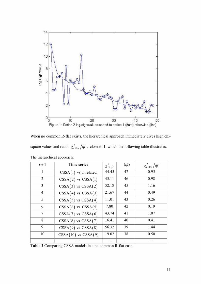
11

When no common R-flat exists, the hierarchical approach immediately gives high chi-

square values and ratios 21r r dfχ + , close to 1, which the following table illustrates.

The hierarchical approach:

1r + Time series 21r rχ + (df) 2

1r r dfχ + 1 CSSA ( )1 vs unrelated 44.45 47 0.95

2 ( )CSSA 2 vs ( )CSSA 1 45.11 46 0.98

3 ( )CSSA 3 vs ( )CSSA 2 52.18 45 1.16

4 ( )CSSA 4 vs ( )CSSA 3 21.67 44 0.49

5 ( )CSSA 5 vs ( )CSSA 4 11.01 43 0.26

6 ( )CSSA 6 vs ( )CSSA 5 7.80 42 0.19

7 ( )CSSA 7 vs ( )CSSA 6 43.74 41 1.07

8 ( )CSSA 8 vs ( )CSSA 7 16.41 40 0.41

9 ( )CSSA 9 vs ( )CSSA 8 56.32 39 1.44

10 ( )CSSA 10 vs ( )CSSA 9 19.02 38 0.50

-- -- -- -- -- Table 2 Comparing CSSA models in a no common R-flat case.

12

In section 6 an example is given where two times series will be analyzed by using

CSSA sharing common properties and a common R-flat of dimension r.

6. Examples

Example 1

The well known Lydia Pinkham annual advertising and sales dataset from 1907 to

1960 is used as a first example. (Data W12 of Wei 2006).

Figure 2 Time series plot for the Advertising and Sales data.

Using the heuristic method, the CPC-eigenvalues of the scatter matrices S1 and S2

were arranged according to the sequence in S1. The eigenvalues of series 2 are

descending up to 5d = , so r can be chosen in the interval 1 5r≤ ≤ .

r Eigenvalues for time series 1 Eigenvalues for time series 2 1 30519735.66 94225252.53 2 20941334.05 71111830.77 3 5064088.50 11134196.86 4 3772917.66 2179336.42 5 3457664.59 1447251.44 6 2573748.36 5240595.10 7 1868804.60 2588007.08 8 1037291.96 846631.05 9 487195.37 267719.61

10 401720.08 182911.91 11 275363.64 312517.49 12 219246.44 327039.47

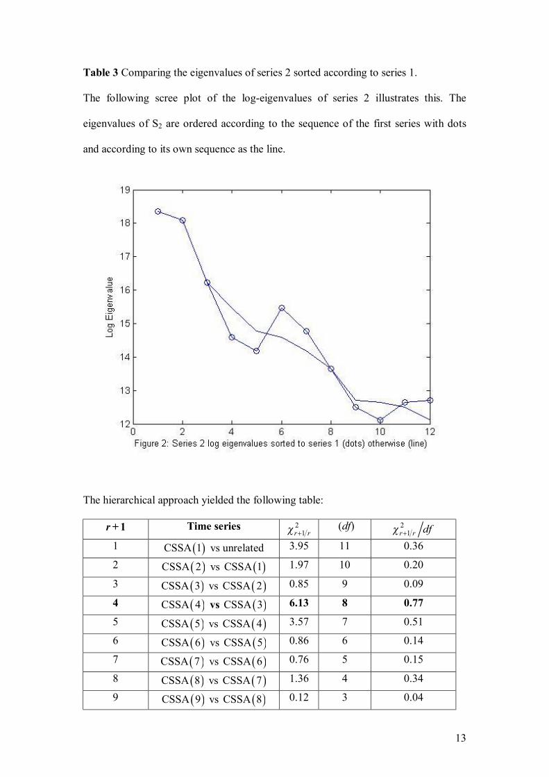
13

Table 3 Comparing the eigenvalues of series 2 sorted according to series 1.

The following scree plot of the log-eigenvalues of series 2 illustrates this. The

eigenvalues of S2 are ordered according to the sequence of the first series with dots

and according to its own sequence as the line.

The hierarchical approach yielded the following table:

1r + Time series 21r rχ + (df) 2

1r r dfχ + 1 CSSA ( )1 vs unrelated 3.95 11 0.36

2 ( )CSSA 2 vs ( )CSSA 1 1.97 10 0.20

3 ( )CSSA 3 vs ( )CSSA 2 0.85 9 0.09

4 ( )CSSA 4 vs ( )CSSA 3 6.13 8 0.77

5 ( )CSSA 5 vs ( )CSSA 4 3.57 7 0.51

6 ( )CSSA 6 vs ( )CSSA 5 0.86 6 0.14

7 ( )CSSA 7 vs ( )CSSA 6 0.76 5 0.15

8 ( )CSSA 8 vs ( )CSSA 7 1.36 4 0.34

9 ( )CSSA 9 vs ( )CSSA 8 0.12 3 0.04

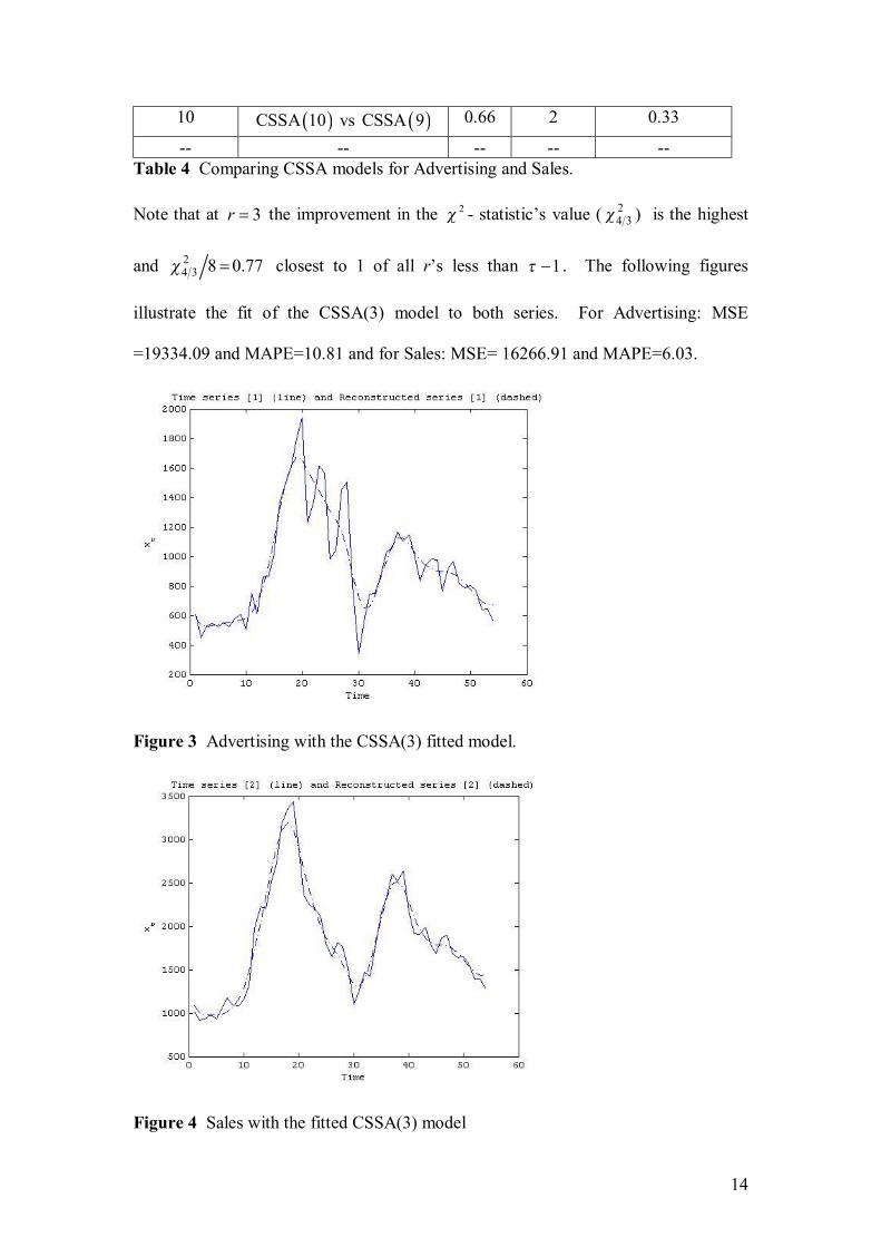
14

10 ( )CSSA 10 vs ( )CSSA 9 0.66 2 0.33

-- -- -- -- -- Table 4 Comparing CSSA models for Advertising and Sales.

Note that at 3r = the improvement in the 2χ - statistic’s value ( 24 3χ ) is the highest

and 24 3 8 0.77χ = closest to 1 of all r’s less than 1τ − . The following figures

illustrate the fit of the CSSA(3) model to both series. For Advertising: MSE

=19334.09 and MAPE=10.81 and for Sales: MSE= 16266.91 and MAPE=6.03.

Figure 3 Advertising with the CSSA(3) fitted model.

Figure 4 Sales with the fitted CSSA(3) model

15

These series are quite short and the CSSA fit is rather rough. The following example

gives a CSSA fit to two longer economic time series.

Example 2

The Business Cycle index (BCI) for South Africa and New car sales index (NCI) is

studied for the period January 1960 till December 2004. Both series are linearly

increasing and co-integrated according to the Johansen test. (Johansen (1988).

According to the Granger test, BCI is the leading indicator. BCI was chosen as

indicated as series 1 and NCI as series 2.

Figure 5 Time series plot for the Business Cycle Index and New Car Sales Index

From the heuristic method, the CPC-eigenvalues of the scatter matrices S1 and S2

were arranged according to the sequence in S1. The eigenvalues of series 2 are then

descending up to 8d = , so r can be chosen as 1 8r≤ ≤ .

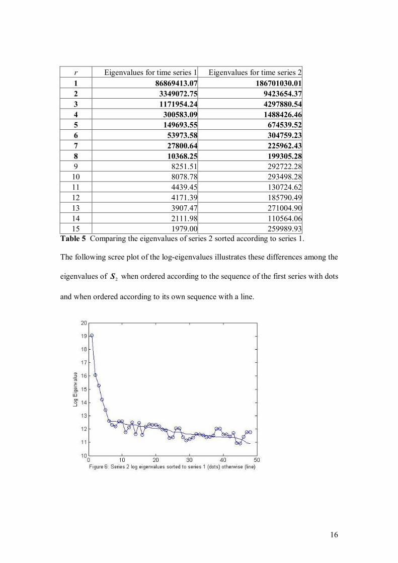
16

r Eigenvalues for time series 1 Eigenvalues for time series 2 1 86869413.07 186701030.01 2 3349072.75 9423654.37 3 1171954.24 4297880.54 4 300583.09 1488426.46 5 149693.55 674539.52 6 53973.58 304759.23 7 27800.64 225962.43 8 10368.25 199305.28 9 8251.51 292722.28

10 8078.78 293498.28 11 4439.45 130724.62 12 4171.39 185790.49 13 3907.47 271004.90 14 2111.98 110564.06 15 1979.00 259989.93

Table 5 Comparing the eigenvalues of series 2 sorted according to series 1.

The following scree plot of the log-eigenvalues illustrates these differences among the

eigenvalues of 2S when ordered according to the sequence of the first series with dots

and when ordered according to its own sequence with a line.

17

Figure 6 illustrates the descending order among the eigenvalues of series 2 for the

different orderings and indicates a ‘fit’ of the CSSA(r) model for a value of r of about

7.

The hierarchical approach yields:

1r + Time series 21r rχ + (df) 2

1r r dfχ + 1 CSSA ( )1 vs unrelated 8.26 47 0.18

2 ( )CSSA 2 vs ( )CSSA 1 3.67 46 0.08

3 ( )CSSA 3 vs ( )CSSA 2 6.21 45 0.14

4 ( )CSSA 4 vs ( )CSSA 3 2.66 44 0.06

5 ( )CSSA 5 vs ( )CSSA 4 3.54 43 0.08

6 ( )CSSA 6 vs ( )CSSA 5 8.40 42 0.20

7 ( )CSSA 7 vs ( )CSSA 6 8.99 41 0.22

8 ( )CSSA 8 vs ( )CSSA 7 45.61 40 1.14

9 ( )CSSA 9 vs ( )CSSA 8 9.02 39 0.23

10 ( )CSSA 10 vs ( )CSSA 9 11.93 38 0.31

-- -- -- -- -- Table 6 Comparing CSSA models for BCI and NCS.

Note that at 7r = the improvement in the 2χ - statistic’s value ( 28 7χ ) is the highest

and 28 7 40 1.14χ = closest to 1 of all r’s less than 1τ − . The following figures

illustrate the fit of the CSSA(7) model fits for both time series.

Figure 7 The Business Cycle Index with the CSSA(7) fitted model.

18

Figure 8 The New Car Sales Index with the fitted CSSA(7) model

The MSE = 2.99 and MAPE=0.58 for the Business Cycle Index and the MSE=226.20

and MAPE=3.27 for the New Car Sales Index.

7 Co-integration and CSSA.

Two time series of length 100T = were simulated to investigate common properties

with CSSA and co-integration:

( )( )

21 1 1 1 1 1 1 1 1

22 2 2 2 2 2 2 2 2

cos sin

cos sin

y t A t B t c d t e t

y t A t B t c d t e t

ω ω ε

ω ω ε

= + + + + +

= + + + + +

where andi iA B are the amplitudes , andi i ic d e , parameters for a polynomial model

and iε a random value drawn from a normal distribution with mean 0 and variance 1

multiplied by a constant amount ni to enlarge the noise level for each time series

( )iy t , where 2i ifω π= and 1i if P= where Pi is the periodicity of each time series

for 1,2i = .

Different values for andi iA B , , andi i ic d e where chosen and the noise levels ni were

also increased to reflect differences between the series.

19

In the investigation process the scree plot of the log eigenvalues of series 2 sorted to

series 1 is considered. The chosen value of r ( )0 r d< ≤ , among the number d of

descending singular values is then reported. If the scree plot indicate common

decreasing log eigenvalues as in the examples given in section 6, Figures 2 and 6

with only minute differences among these eigenvalues of series 2, it will indicate “fit”

of the CSSA model meaning that common features exist . In Figure 1 (see section 6)

the scree plot indicates a “non-fit”, meaning that no common features exist. In Table

2 the hierarchical method indicates a “non-fit” characterized by immediate high chi-

square values and ratios 21r r dfχ + , close to 1.

To avoid the further use of too many scree plots or tables, we will simply refer to a fit

or a non-fit of the CSSA model. In the following section several scenarios are

investigated to access the fit of the CSSA model. The scree plots of the log

eigenvalues are investigated like mentioned above and the mean squared errors and

mean absolute percentage errors of the fitted series are calculated and reported as

MSE1, MSE2 and MAPE1, MAPE2 respectively for each scenario.

6.1 Investigating the window length for different values ofτ :

The values for the slopes 1 2andd d where chosen as 0.5 while the following values

where chosen for the intercepts and polynomial terms 1 2 1 210, 0c c e e= = = = , the

amplitudes 1 1 2 2 5A B A B= = = = and the period of the time series Pi =12. The noise

constants where chosen as 0.5. The two time series are therefore positive linear and

sinusoidal. When using 12τ = it was found that the window length is too short to

detect the similarity between the two series and consequently the window length was

extended to 48τ = . The number of mutually decreasing eigenvalues was determined

as 5d = which yielded scree plots indicating fit. Consequently 4r = is chosen for

20

the CSSA reconstruction. The reconstructed time series now fit the original time

series with respective error measures MSE1 =0.16, MAPE1 =1.30 and MSE2=0.20,

MAPE2=1.27. Since a window length of 48τ = gives a better fit, this window length

is chosen for all further comparisons.

6.2 Influence of different slopes: Different slopes involve choosing different

values of 1 2andd d . The starting values given in (a) below are 1 20.5 and 0.6d d= =

while the other components are chosen as:

1 2 1 2 1 1 2 2 1 210, 0, 5 and12

c c e e A B A B πω ω= = = = = = = = = = .

The noise constants were chosen as 0.5. In (a) the two slopes are almost similar, (b)

gives the results when the slope of the one time series is linear positive and the second

one linear negative. In (c) the slope of the first time series is linear positive but the

second one is stationary. Note that in this case the series are not co-integrated.

(a) The slopes for the two time series are 1 0.5d = and 2 0.6d = . The number of

similarly ordered eigenvalues from CSSA is determined as 4d = . The scree

plots indicate fit and using 4r = resulted in MSE1=0.16, MAPE1=1.12,

MSE2=0.21 and MAPE2=1.24. Using the hierarchical approach, 4r = .

(b) The slopes were chosen as 1 0.5d = and 2 2d = − . The number of ordered

eigenvalues from CSSA is 6d = . The scree plots indicate fit and the use of

4r = resulted in fits with MSE1 =0.18, MAPE1=1.29, MSE2=0.25 and

MAPE2=0.98. The hierarchical approach yielded, 4r = .

(c) The slopes where chosen as 1 0.5d = and 2 0d = . The number of ordered

eigenvalues is 1d = which immediately indicate non-fit of the CSSA model.

This is also clear from the scree plots and by comparing the MSE’s and

MAPE’s after the CSSA model is fitted. Using 1r = results in MSE1=24.59,

21

MAPE1=17.12, MSE2=24.22 and MAPE2=68.82. The Hierarchical approach

indicates a non-fit. Immediate high chi-square values and ratios 21r r dfχ + ,

close to 1 ( as in Table 1) is obtained.

Note that the two series in (a) and (b) are both first order non-stationary and the CSSA

model fits, indicated by the small MSE’s and MAPE’s. It seems that a difference in

the slopes when both series are first order non-stationary does not influence the fit of

the CSSA model, though it influences co-integration. However in (c) the one series is

first order non-stationary while the second one is stationary. In this case the series are

not co-integrated but the CSSA model also does not fit.

6.3 Influence of different quadratic components: In the following analysis (a)

the values for the linear coefficients are fixed on 1 2 0.5d d= = but the quadratic

coefficients are chosen as 1 0e = and 2 0.05e = . Thus the one time series has a linear

trend while the other one has a quadratic trend. The noise variance is chosen as 0.5,

while the other components were chosen as 1 2 10c c= = , 1 1 2 2 5A B A B= = = =

and 1 2 12πω ω= = . In the analysis (b) the linear coefficients are changed to 1 0.5d =

and 2 2d = − resulting in a negative linear series 2 being also perpendicular to series 1.

(a) The quadratic components were chosen as 1 0.05e = and 2 0e = . The number

of ordered eigenvalues is 2d = . Using 2r = yielded the following fitted

series with CSSA: MSE1 =13.35, MAPE1=7.00, MSE2 = 11.31 and

2MAPE =12.68 . From the hierarchical approach, 3r = .

(b) The slopes were chosen as 1 0.5d = , 2 2d = − and the quadratic components as

1 0.05e = and 2 0e = . The ordered eigenvalues 3d = . The Hierarchical

approach gives immediate high chi-square values indicating a non-fit.

22

Choosing 3r = both the scree plot and the error measures MSE1=9.70,

MAPE1=7.20, 2MSE =86.92 and MAPE2 = 42.98 also indicate no fit.

In both cases (a) and (b) the large MAPE’s indicate bad fit, particularly for the second

case as in (b). Note that since the one series is linear, i.e. of order I(1) and the other

quadratic of order I(2), they are not co-integrated and the CSSA model does not fit.

6.4 Influence of periodicity on CSSA: The periods of the two time series,

1 2andω ω were chosen as different, 1 12π

ω = and 2 6πω = while the other

components were chosen the same, 1 1 2 2 5A B A B= = = = , 1 2 10c c= = , 1 2 0.5d d= = ,

1 2 0e e= = and noise constant 0.5. Three ordered eigenvalues ( 3d = ) were

observed. Using 3r = and fitting the CSSA model resulted in MSE1=0.21,

MAPE1=1.31, MSE2=25.50 and MAPE2=18.09. The Hierarchical approach indicates

a non-fit of the CSSA model due to immediate large chi-square values. This is also

visible from the scree plot and larger MSE and MAPE of the second series. Since the

two series are however co-integrated according to the Johansen (1991) test, this

illustrates that co-integration not necessarily imply that the CSSA model will fit. Thus

CSSA is a stronger condition or measure of similarity between two time series than

co-integration.

6.5 Influence of different amplitudes on CSSA: Different amplitudes were given to

the two time series. The time lag k, was set to 0 and the other components were

chosen as 1 2 0.5d d= = , 1 2 0e e= = , 1 2 10c c= = and 1 2 12πω ω= = .

(a) The amplitudes were chosen as 1 1 5A B= = , 2 2 7A B= = . The ordered

eigenvalues indicate 6d = . The scree plot indicate fit and when choosing

23

5r = , the following error measures were found MSE1=0.18, MAPE1=1.23,

MSE2=0.22 and MAPE2= 1.54. Using the hierarchical approach 5r = .

(b) The amplitudes were chosen as 1 1 5A B= = and 2 2 15A B= = . The number of

ordered eigenvalues is 1d = , which immediately indicates a non-fit, even

without plotting any scree plot. If the CSSA model is fitted the error

measures are MSE1=25.03, MAPE1=17.38, MSE2=222.74 and

MAPE2=224.51, confirming the bad fit. The hierarchical approach’s large

chi-square values also confirm the non-fit.

For ratios of amplitudes 2 1A A and 2 1B B close to one, the CSSA model gives a good

fit, but when these amplitude ratios get larger, the CSSA model does not fit. In both

cases (a) and (b) the two series are still co-integrated.

8. CONCLUDING

Common singular value decomposition can be used to investigate common structure

among different time series. The common structure is explained in terms of the r

singular values resulting from the common submatrix : rτ ×B in the matrix/matrices

( )2 ( ) ( )1 1 , 1,2i i

i i r rb b b b iτ+ = = = β … …B B , used to simultaneously

diagonalize the scatter matrices i i′% %X X to CPC or CPC(r ) structure in the Flury-

Gautschi sense, where ( )1,2i i =%X are the respective centered trajectory matrices.

These vectors are the base vectors of the common R-flat. Failure to simultaneously

diagonalize these matrices with CPC or CPC(r) indicates that no common structure

exists at all and thus no common R-flat exists.

CSSA gives more insight into the nature and dimensionality of common features

among time series than co-integration alone.

24

REFERENCES

Broomhead, D.S. and King, G.P.,1986a. Extracting qualitative dynamics from

experimental data. Physica D 20, 217-236.

Broomhead, D.S. and King, G.P., 1986b. On the qualitative analysis of

experimental dynamical systems. In S. Sarkar (Ed.), Non-linear phenomena and

chaos. 113-144. Adam Hilger, Bristol.

Buchstaber, V.M., 1994. Time series analysis and Grassmannians. Amer. Math.

Soc. Transl 162 Series 2, 1-17.

Danilov, D.L., 1997. Principal components in time series forecast. Journal of

computational and Graphical Statistics, 6, 112-121.

Elsner, J.B. and Tsonis, A.A., 1996. Singular Spectrum Analysis. A New Tool in

Time Series Analysis. New York: Plenum Press.

Engle, R.F. and Granger, C.W.J., 1987. Co-integration and error correction:

representation, estimation and testing. Econometrica 55, 251-276.

Flury, B., 1984. Common principal components in k groups. Journal of the

American Statistical Association 79, 892-898.

Flury, B., 1988. Common principal components and related multivariate models.

New York: Wiley.

Flury, B. and Gautschi, W., 1986. An algorithm for simultaneous orthogonal

transformation of several positive definite symmetric matrices to nearly diagonal

form. SIAM Journal of Scientific and Statistical Computing 7, 184-196.

Golyandina, N., Nekrutkin, V.V. and Zhigljavsky, A., 2001. Analysis of Time

series Structure SSA and Related Techniques. Boca Raton, Chapman &

Hall/CRC.

25

Johansen, S., 1988. Statistical analysis of cointegration vectors. Journal of

Economic Dynamics and Control 12, 231-254.

Johansen, S., 1991. Estimation and hypothesis testing of cointegration vector in

Gaussian vector autoregressive models. Econometrica 59, 1551-1580.

Vautard, R., Yiou, P. and Ghil, M. 1992. Singular-spectrum analysis: A toolkit

for short, noisy chaotic signals. Physica D, 58, 95-126.

Venter, J.H., 1998. Forecasting by identification of linear structure in a time

series. Unpublished talk presented at the 1998 Conference of The South-Africa

Statistical Association.

Viljoen, H and Nel D.G., 2009. Common singular spectrum analysis of several

time series. Journal of Statistical Planning and Inference (In press)

Wei, W.W.S., 2006. Time Series Analysis: Univariate and Multivariate Methods.

(Sec. Ed.) Boston: Pearson Addison Wesley.