A Test Matrix Collection forNon-Hermitian Eigenvalue Problems�(Release 1.0)Zhaojun Baiy and David Dayz and James Demmelx and Jack Dongarra{October 6, 19961 IntroductionThe primary purpose of this collection is to provide a testbed for the development of nu-merical algorithms for solving nonsymmetric eigenvalue problems. In addition, as withmany other existing collections of test matrices, our goal includes providing an easy ac-cess to \practical" eigenproblems for researchers, educators and students in the communitywho are interested in the origins of large scale nonsymmetric eigenvalue problems, and inthe development and testing of numerical algorithms for solving challenging non-Hermitianeigenvalue problems in real applications.In this document, we describe the mechanism for obtaining a copy of the matrices and forusing the collection. All test matrices currently included in the collection are documentedin Appendices.2 Organziation of the collectionThere are four directories in the collection:� document/ contains the postscript �le of this report and the postrscript �les of picturesincluded in the docuement.� utility/ contains the utility routines in FORTRAN, C and Matlab M-�les for basicmanilpulations and computations of the matrices included in this collection, such asread or write a sparse matrix in the HB format, matrix-vector multiplication etc.� data/ contains the data �les of test matrices which are presented in the standardHarwell-Beoing format.�This work was supported in part by NSF grant ASC-9313958 and in part by DOE grant DE-FG03-94ER25219.yDepartment of Mathematics, University of Kentucky, Lexington, KY 40506.zMS 1110, Sandia National Laboratories PO Box 5800, Albuquerque, NM 87185.xComputer Science Division and Mathematics Department, University of California, Berkeley, CA 94720.{Department of Computer Science, University of Tennessee, Knoxville, TN 37996 and MathematicalSciences Section, Oak Ridge National Laboratory, Oak Ridge, TN 37831.1

� matsrc/ contains the test matrices which are presented in the matrix-vector productformat or in the subroutine format.3 How to obtain the collectionThe entire collection (document, software and data) is available through direct electronictransfer on the MatrixMarket, a web resource for test matrix collections. The URL of theMatrrixMarket is http://math.nist.gov/MatrixMarket.4 Matrix Formats and UsageThere are three formats in which to represent the sparse matrices in the collection, namelythe standard Harwell-Boeing (HB) sparse matrix format, the matrix-vector multiplicationformat, and the subroutine format.4.1 HB Sparse compressed column formatThe matrices stored in data �les are stored in sparse column format (i.e., standard Harwell-Boeing format).1 Utility routines dreadm.f and dprtmt.f can be used for reading or writinga real sparse matrix in this format in FORTRAN. zreadm.f and zprtmt.f are complexversions. dreadhb.c is the C version. Matlab M-�les dm2hb.m and zm2hb.m can be used towrite a real and complex sparse matrices in MATLAB to the HB format, respectively.The following is a brief summary of the compressed column storage scheme. For moredetails, see the User's Guide for the Harwell-Boeing Sparse Matrix Collection.In any sparse matrix format only the non-zero entries of a matrix are stored. An entryis speci�ed by its row index, column index, and value. In sparse column format a singleinteger array and a single oating point array are used to store the row indices and thevalues, respectively, for all columns. The data for each column are stored in consecutivelocations, the columns are stored in order, and there is no space between columns. An otherinteger array points to the �rst entry in each column.The sparse matrix A of order n and with nnz non-zero entries is represented by a oatingpoint array a(1 : nnz) that stores the values, an integer array ia(1 : nnz) that stores therow indices, and an integer array ja(1 : n+ 1) with the property that ja(k + 1)� 1 pointsto the last element in column k.4.2 Matrix-vector multiplication formatSome of test matrices in this collection are presented in a di�erent format than the standardHarwell-Boeing format. Instead of storing the matrix in a data �le, the matrix is representedas a subroutine that computes the matrix-vector multiplications AX and/orATX for a givenX , where X is a single vector or a block vector (matrix). These matrices are of variablesize, and often depend on parameters that in uence the eigenvalues.1I. S. Du�, R. G. Grimes and J. G. Lewis, User's Guide for the Harwell-Boeing Sparse Matrix Collection(Release I), CERFACS, TR/PA/92/86, Oct. 1992. It is available via anonymous ftp: orion.cerfacs.fr, cdpub/harwell boeing. 2

4.3 Subroutine formatIn subroutine format the user generates a matrix of speci�ed order (and parameter valuesif applicable) represented in compressed column or compressed row format. The matrixis stored in two integer arrays and one real array. Routines for performing matrix-vectorproducts etc. are available in the utilities directory of the collection.5 Acknoledgement and contributing to the collectionThis work is in fact a compilation of e�orts of many people. Their names will be acknowl-edged with the asscoiated matrices in the collection. We will keep updating the collectionas new test problems become available. At a proper time, we plan to record performancedata of di�erent numerical methods and chanllenges associated with these test problems.Your comments and contributions are welcomed. Please contact Bai by sending elec-tronic mail to bai@ms.uky.edu or by writing to: Department of Mathematics, University ofKentucky, Lexington, KY 40506, USA.Appendix A: Matrices in Standard HB Sparse Matrix FormatAppendix B: Matrices in Matrix-Vector Product FormatAppendix C: Matrices in Subroutine FormatAppendix D: List of Utility Routines

3

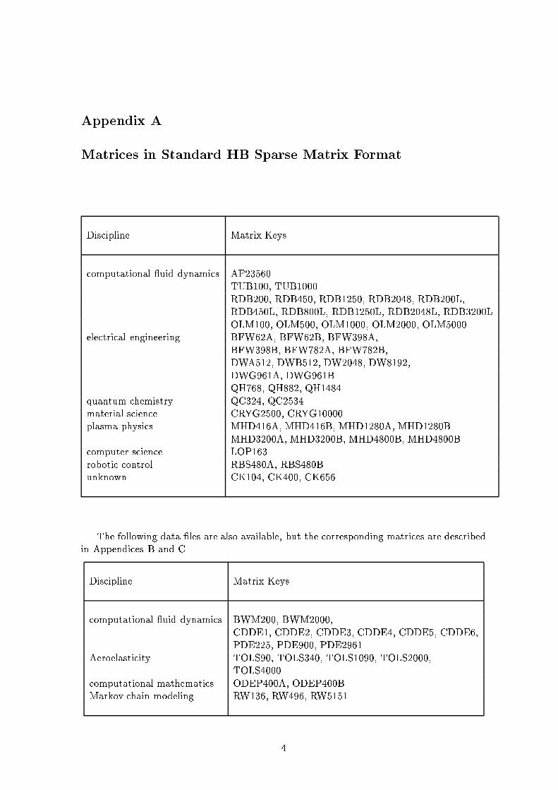
Appendix AMatrices in Standard HB Sparse Matrix FormatDiscipline Matrix Keyscomputational uid dynamics AF23560TUB100, TUB1000RDB200, RDB450, RDB1250, RDB2048, RDB200L,RDB450L, RDB800L, RDB1250L, RDB2048L, RDB3200LOLM100, OLM500, OLM1000, OLM2000, OLM5000electrical engineering BFW62A, BFW62B, BFW398A,BFW398B, BFW782A, BFW782B,DWA512, DWB512, DW2048, DW8192,DWG961A, DWG961BQH768, QH882, QH1484quantum chemistry QC324, QC2534material science CRYG2500, CRYG10000plasma physics MHD416A, MHD416B, MHD1280A, MHD1280BMHD3200A, MHD3200B, MHD4800B, MHD4800Bcomputer science LOP163robotic control RBS480A, RBS480Bunknown CK104, CK400, CK656The following data �les are also available, but the corresponding matrices are describedin Appendices B and C.Discipline Matrix Keyscomputational uid dynamics BWM200, BWM2000,CDDE1, CDDE2, CDDE3, CDDE4, CDDE5, CDDE6,PDE225, PDE900, PDE2961.Aeroelasticity TOLS90, TOLS340, TOLS1090, TOLS2000,TOLS4000.computational mathematics ODEP400A, ODEP400B.Markov chain modeling RW136, RW496, RW5151.4

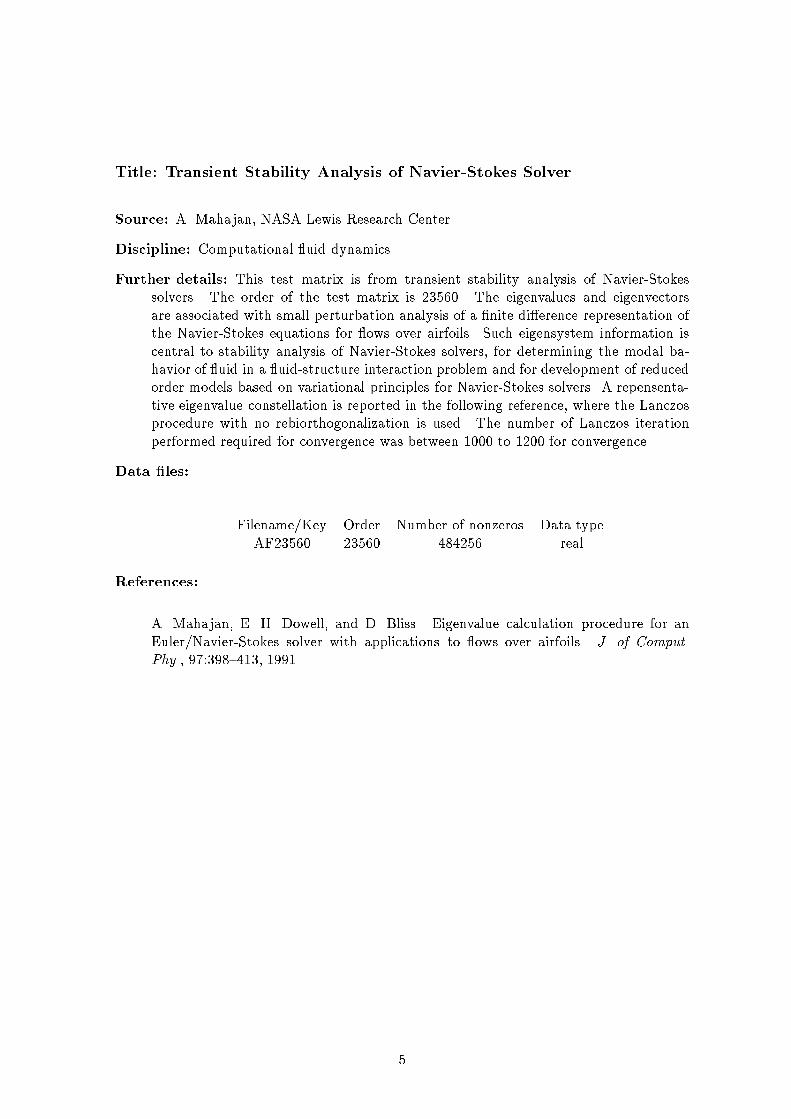
Title: Transient Stability Analysis of Navier-Stokes SolverSource: A. Mahajan, NASA Lewis Research CenterDiscipline: Computational uid dynamicsFurther details: This test matrix is from transient stability analysis of Navier-Stokessolvers. The order of the test matrix is 23560. The eigenvalues and eigenvectorsare associated with small perturbation analysis of a �nite di�erence representation ofthe Navier-Stokes equations for ows over airfoils. Such eigensystem information iscentral to stability analysis of Navier-Stokes solvers, for determining the modal ba-havior of uid in a uid-structure interaction problem and for development of reducedorder models based on variational principles for Navier-Stokes solvers. A repensenta-tive eigenvalue constellation is reported in the following reference, where the Lanczosprocedure with no rebiorthogonalization is used. The number of Lanczos iterationperformed required for convergence was between 1000 to 1200 for convergence.Data �les: Filename/Key Order Number of nonzeros Data typeAF23560 23560 484256 realReferences:A. Mahajan, E. H. Dowell, and D. Bliss. Eigenvalue calculation procedure for anEuler/Navier-Stokes solver with applications to ows over airfoils. J. of Comput.Phy., 97:398{413, 1991.

5

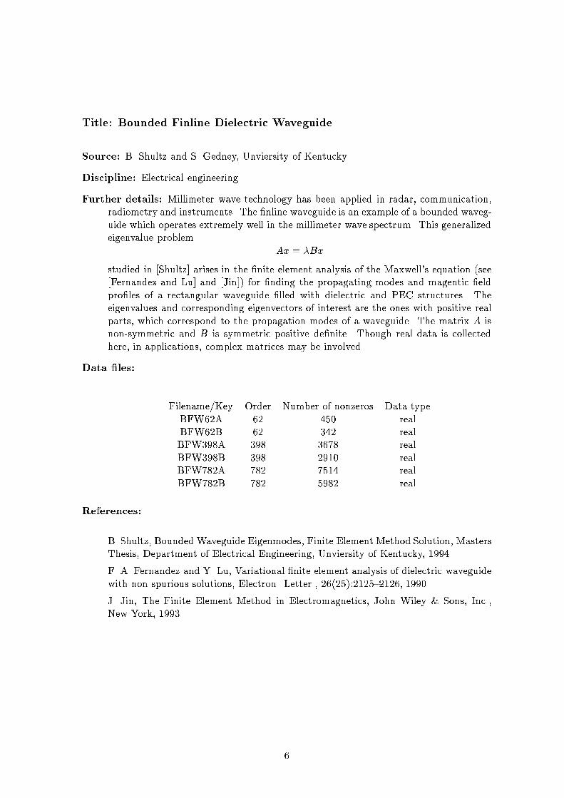
Title: Bounded Finline Dielectric WaveguideSource: B. Shultz and S. Gedney, Unviersity of KentuckyDiscipline: Electrical engineeringFurther details: Millimeter wave technology has been applied in radar, communication,radiometry and instruments. The �nline waveguide is an example of a bounded waveg-uide which operates extremely well in the millimeter wave spectrum. This generalizedeigenvalue problem Ax = �Bxstudied in [Shultz] arises in the �nite element analysis of the Maxwell's equation (see[Fernandez and Lu] and [Jin]) for �nding the propagating modes and magentic �eldpro�les of a rectangular waveguide �lled with dielectric and PEC structures. Theeigenvalues and corresponding eigenvectors of interest are the ones with positive realparts, which correspond to the propagation modes of a waveguide. The matrix A isnon-symmetric and B is symmetric positive de�nite. Though real data is collectedhere, in applications, complex matrices may be involved.Data �les: Filename/Key Order Number of nonzeros Data typeBFW62A 62 450 realBFW62B 62 342 realBFW398A 398 3678 realBFW398B 398 2910 realBFW782A 782 7514 realBFW782B 782 5982 realReferences:B. Shultz, Bounded Waveguide Eigenmodes, Finite Element Method Solution, MastersThesis, Department of Electrical Engineering, Unviersity of Kentucky, 1994.F. A. Fernandez and Y. Lu, Variational �nite element analysis of dielectric waveguidewith non spurious solutions, Electron. Letter., 26(25):2125{2126, 1990.J. Jin, The Finite Element Method in Electromagnetics, John Wiley & Sons, Inc.,New York, 1993.6

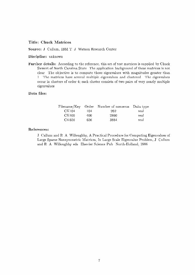
Title: Chuck MatricesSource: J. Cullum, IBM T. J. Watson Research CenterDiscipline: unknownFurther details: According to the reference, this set of test matrices is supplied by ChuckSiewert of North Carolina State. The application background of these matrices is notclear. The objective is to compute those eigenvalues with magnitudes greater than1. The matrices have several multiple eigenvalues and clustered. The eigenvaluesoccur in clusters of order 4; each cluster consists of two pairs of very nearly multipleeigenvalues.Data �les: Filename/Key Order Number of nonzeros Data typeCK104 104 992 realCK400 400 2860 realCK656 656 3884 realReferences:J. Cullum and R. A. Willoughby, A Practical Procedure for Computing Eigenvalues ofLarge Sparse Nonsymmetric Matrices, In Large Scale Eigenvalue Problem, J. Cullumand R. A. Willoughby eds. Elsevier Science Pub. North-Holland, 1986.

7

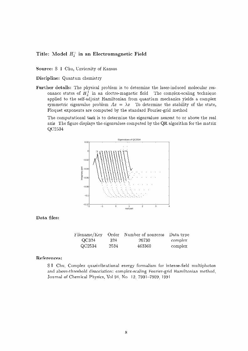
Title: Model H+2 in an Electromagnetic FieldSource: S. I. Chu, Unviersity of KansasDiscipline: Quantum chemistryFurther details: The physical problem is to determine the laser-induced molecular res-onance states of H+2 in an electro-magnetic �eld. The complex-scaling techniqueapplied to the self-adjoint Hamiltonian from quantium mechanics yields a complexsymmetric eigenvalue problem Ax = �x. To determine the stability of the state,Floquet exponents are computed by the standard Fourier-grid method.The computational task is to determine the eigenvalues nearest to or above the realaxis. The �gure displays the eigenvalues computed by the QR algorithm for the matrixQC2534.−2 −1 0 1 2 3 4

−0.12

−0.1

−0.08

−0.06

−0.04

−0.02

0

0.02

real part

imag

inar

y pa

rt

Eigenvalues of QC2534

Data �les: Filename/Key Order Number of nonzeros Data typeQC324 324 26730 complexQC2534 2534 463360 complexReferences:S.I. Chu, Complex quasivibrational energy formalism for intense-�eld multiphotonand above-threshold dissociation: complex-scaling Fourier-grid Hamiltonian method,Journal of Chemical Physics, Vol.94, No. 12, 7901{7909, 1991.8

Title: DI�usion Model Study for Crystal Growth SimulationSource: C. Yang, Rice UniversityDiscipline: Material ScienceFurther details This is a large nonsymmetric standard eigenvalue problem that arisesfrom the stability analysis of a crystal growth problem. To determine the stabil-ity of the interfacial crystallization of a piece of solid crystal solidifying into someundercooled melt, solutions of the following equations are sought.1�2 + �2�@2U@�2 + @2U@�2 + 2P��@U@� � � @U@� �� = �U;�11 + �2 �@U@� + 4P 2N + 2P (N + � @N@� )� = �N;U = 2PN at � = 1:Zero Dirichlet boundary condition is imposed at in�nity. The variable U in the aboveequations represents the temperature perturbation of the liquid, and N describes theinterface perturbation in a transformed (parabolic) coordinate system. The constantP is the Peclet number. The second equation is satis�ed only at the interface � = 1.Eigenvalues with largest real parts are of interest. They indicate the growth or decay ofthe initial disturbance at the solid-liquid interface. A change of variable is used to mapthe partial di�erential equation from an in�nite domain to a �nite box [0; 1]� [1; 2].The matrix eigenvalue problem follows from discretization using the standard secondorder �nite di�erence formulae. The Peclet number used here is P = 0:05.Data �les: Filename/Key Order Number of nonzeros Data typeCRYG2500 2500 12349 realCRYG10000 10000 49699 realReferences:C. Yang, D. C. Sorensen, D. I. Meiron and B. Wedeman, Numerical Computation ofthe Linear Stability of the Di�usion Model for Crystal Growth Simulation, TechnicalReport, TR96-04, Department of Comp & Applied Mathematics, Rice University,1996.9

Title: Square Dielectric WaveguideSource: H. Dong, Unviersity of MinnesotaDiscipline: Electrical engineeringFurther details: Dielectric channel waveguide problems arise in many integrated circuitapplications. Finite di�erence discretization of the governing Helmholtz equation forthe magnetic �eld H , r2Hx + k2n2(x; y)Hx = �2Hx;r2Hy + k2n2(x; y)Hy = �2Hy;leads to the nonsymmetric eigenvalue problem of the form C11 C12C21 C22 ! HxHy ! = �2 B11 B22 ! HxHy !where C11 and C22 are �ve- or tri-diagonal matrices, C12 and C21 are (tri-) diago-nal matrices, and B11 and B22 are nonsingular diagonal matrices. This generalizedeigenvalue problem is reduced to a standard eigenvalue problem Ax = x�, whereA = B�1C, since B is diagonal.The computational task is to determine the right most eigenvalues and their corre-sponding eigenvectors. In some cases, there are eigenvalues with negative real partseveral orders of magnitude larger than the desired eigenvalues with positive real part.This problem presents a challenge to existing numerical methods.Data �les: Filename/Key Order Number of nonzeros Data typeDWA512 512 2480 realDWB512 512 2500 realDW2048 2048 10114 realDW8192 8192 41746 realNote that DWA512 and DWB512 are the matrices of same order which correspond todi�erent parameter values.References:H. Dong, A. Chronopoulos, J. Zou and A. Gopinath, Vectorial integrated �nite-di�erence analysis of dielectric waveguides, private communication, 1993A. Galick, T. Kerhoven and U. Ravaioli, Iterative solution of the eigenvalue prob-lem for a dielectric waveguid, IEEE Trans. Microwave Theory Tech. vol. MTT-40,pp.699{705, 1992. 10

Title: Dispersive Waveguide StructuresSource: S. Gedney and U. D. Navsariwala, Unviersity of KentuckyDiscipline: Electrical engineeringFurther details: This is a complex symmetric eigenvalue problem Ax = �Bx, where bothA and B are complex and symmetric, but not Hermitian. Moreover, the matrices Aand B are of the forms A11 00 0 ! and B11 B12B21 B22 ! ;respectively. In the work of Tan and Pan, it is shown that the eigenvalue problemis derived from using the edge element method to solve the waveguide problem ofconductors with �nite conductivity and cross section in a lossy dielectric media. Thematrix size can easily reach a few thousands.The subblock matrix A11 is 705 by 705, and banded. The computational task is to�nd the eigenvalues with the smallest positive real parts.Data �les: Filename/Key Order Number of nonzeros Data typeDWG961A 961 3405 complexDWG961B 961 10591 complexReferences:J. Tan and G. Pan, A new edge element analysis of dispersive waveguiding structures,IEEE trans. on microwave theory and tech. Vol.43, No.11, pp.2600{2607, Nov. 1995.S. Gedney and U. D. Navsariwala, personal communication, 199611

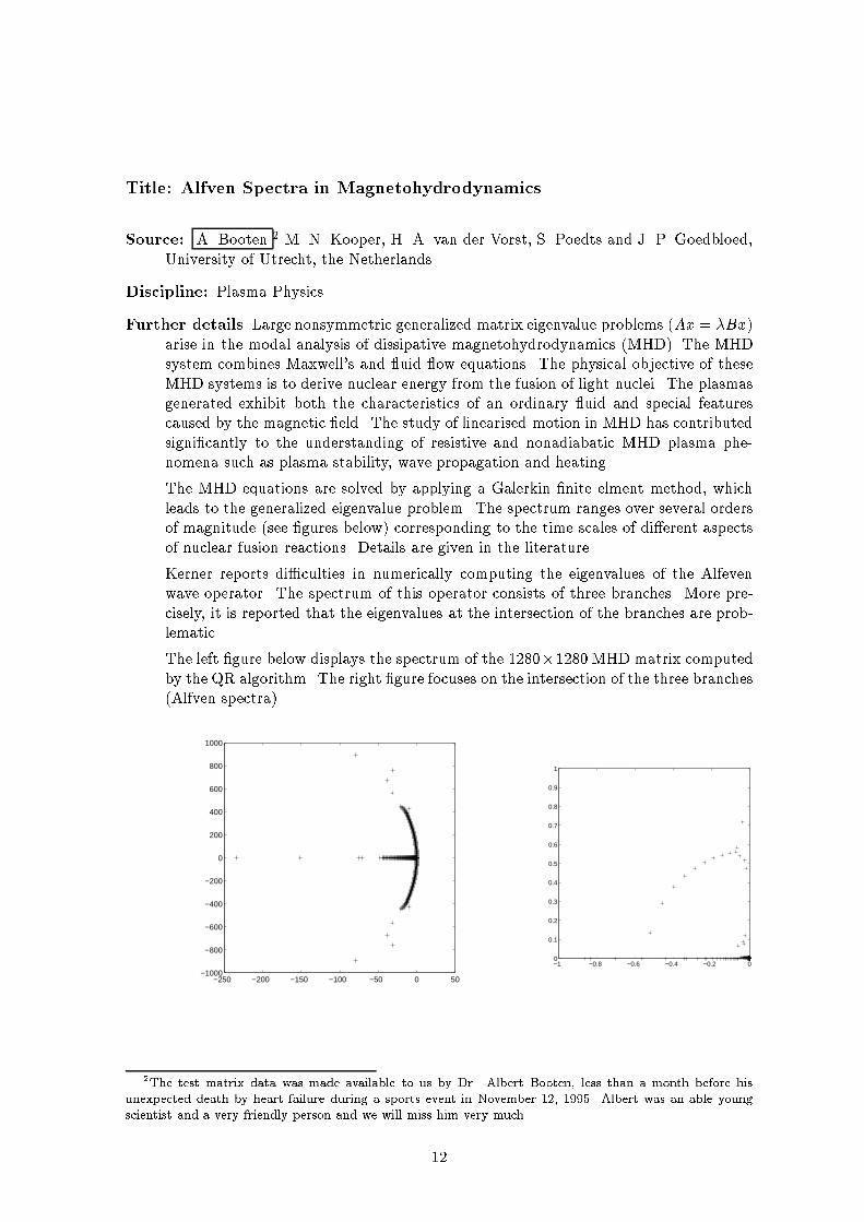
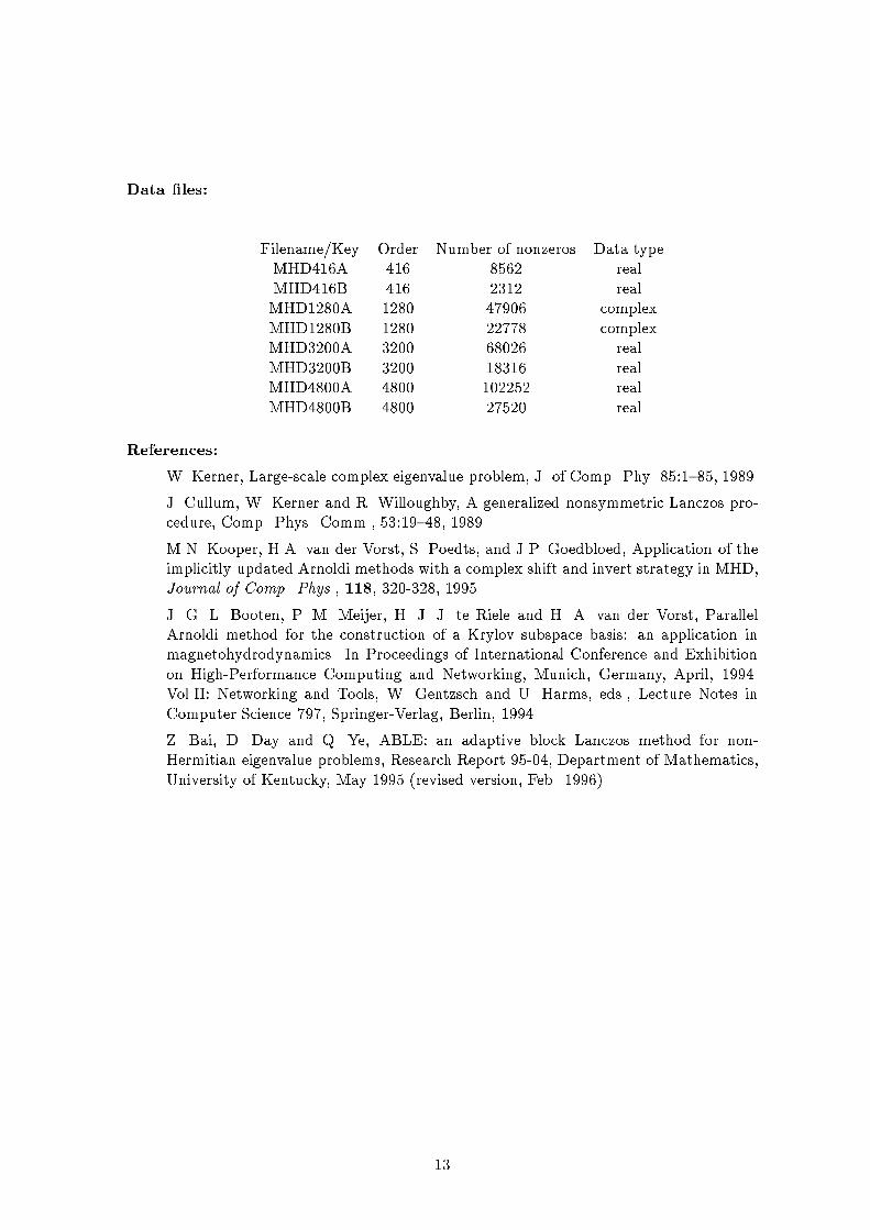
Title: Alfven Spectra in MagnetohydrodynamicsSource: A. Booten 2 M. N. Kooper, H. A. van der Vorst, S. Poedts and J. P. Goedbloed,University of Utrecht, the Netherlands.Discipline: Plasma PhysicsFurther details Large nonsymmetric generalized matrix eigenvalue problems (Ax = �Bx)arise in the modal analysis of dissipative magnetohydrodynamics (MHD). The MHDsystem combines Maxwell's and uid ow equations. The physical objective of theseMHD systems is to derive nuclear energy from the fusion of light nuclei. The plasmasgenerated exhibit both the characteristics of an ordinary uid and special featurescaused by the magnetic �eld. The study of linearised motion in MHD has contributedsigni�cantly to the understanding of resistive and nonadiabatic MHD plasma phe-nomena such as plasma stability, wave propagation and heating.The MHD equations are solved by applying a Galerkin �nite elment method, whichleads to the generalized eigenvalue problem. The spectrum ranges over several ordersof magnitude (see �gures below) corresponding to the time scales of di�erent aspectsof nuclear fusion reactions. Details are given in the literature.Kerner reports di�culties in numerically computing the eigenvalues of the Alfevenwave operator. The spectrum of this operator consists of three branches. More pre-cisely, it is reported that the eigenvalues at the intersection of the branches are prob-lematic.The left �gure below displays the spectrum of the 1280�1280 MHD matrix computedby the QR algorithm. The right �gure focuses on the intersection of the three branches(Alfven spectra).−250 −200 −150 −100 −50 0 50

−1000

−800

−600

−400

−200

0

200

400

600

800

1000

−1 −0.8 −0.6 −0.4 −0.2 00

0.1

0.2

0.3

0.4

0.5

0.6

0.7

0.8

0.9

1

2The test matrix data was made available to us by Dr. Albert Booten, less than a month before hisunexpected death by heart failure during a sports event in November 12, 1995. Albert was an able youngscientist and a very friendly person and we will miss him very much.12

Data �les: Filename/Key Order Number of nonzeros Data typeMHD416A 416 8562 realMHD416B 416 2312 realMHD1280A 1280 47906 complexMHD1280B 1280 22778 complexMHD3200A 3200 68026 realMHD3200B 3200 18316 realMHD4800A 4800 102252 realMHD4800B 4800 27520 realReferences:W. Kerner, Large-scale complex eigenvalue problem, J. of Comp. Phy. 85:1{85, 1989.J. Cullum, W. Kerner and R. Willoughby, A generalized nonsymmetric Lanczos pro-cedure, Comp. Phys. Comm., 53:19{48, 1989M.N. Kooper, H.A. van der Vorst, S. Poedts, and J.P. Goedbloed, Application of theimplicitly updated Arnoldi methods with a complex shift and invert strategy in MHD,Journal of Comp. Phys., 118, 320-328, 1995.J. G. L. Booten, P. M. Meijer, H. J. J. te Riele and H. A. van der Vorst, ParallelArnoldi method for the construction of a Krylov subspace basis: an application inmagnetohydrodynamics. In Proceedings of International Conference and Exhibitionon High-Performance Computing and Networking, Munich, Germany, April, 1994.Vol.II: Networking and Tools, W. Gentzsch and U. Harms, eds., Lecture Notes inComputer Science 797, Springer-Verlag, Berlin, 1994.Z. Bai, D. Day and Q. Ye, ABLE: an adaptive block Lanczos method for non-Hermitian eigenvalue problems, Research Report 95-04, Department of Mathematics,University of Kentucky, May 1995 (revised version, Feb. 1996).13

Title: Quebec Hydroelectric Power SystemKey: QH882Source: Deo Ndereyimana, Quebec, CanadaDiscipline: Power systems simulationsFurther details: This set of matrices is from the application of the Hydro-Quebec powersystems' small-signal model. In the application, one wants to compute all eigenvaluesa + ib in a box of the complex plane. Speci�cally, amin < a < amax and in general,amin = �300 and amax = 300. bmin < b < bmax and in general, bmin = 0 andbmax = 2� 60�. Note that the matrices are highly unbalanced.Data �les: Filename/Key Order Number of nonzeros Data typeQH768 768 2934 realQH882 882 3354 realQH1484 1484 6110 realReferences:Deo Ndereyimana, personal communication, 1994

14

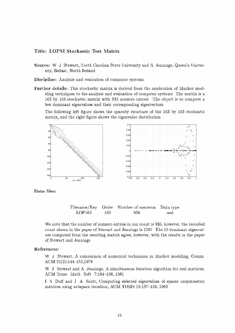
Title: LOPSI Stochastic Test MatrixSource: W. J. Stewart, North Carolina State University and A. Jennings, Queen's Univer-sity, Belfast, North Ireland.Discipline: Analysis and evaluation of computer systemsFurther details: This stochastic matrix is derived from the application of Markov mod-eling techniques to the analysis and evaluation of computer systems. The matrix is a163 by 163 stochastic matrix with 935 nonzero entries. The object is to compute afew dominant eigenvalues and their corresponding eigenvectors.The following left �gure shows the sparsity structure of the 163 by 163 stochasticmatrix, and the right �gure shows the eigenvalue distribution.0 50 100 150

0

20

40

60

80

100

120

140

160

nz = 934-0.8 -0.6 -0.4 -0.2 0 0.2 0.4 0.6 0.8 1

-0.1

-0.08

-0.06

-0.04

-0.02

0

0.02

0.04

0.06

0.08

0.1

Data �les: Filename/Key Order Number of nonzeros Data typeLOP163 163 936 realWe note that the number of nonzero entries in our count is 936, however, the recordedcount shown in the paper of Stewart and Jennings is 1207. The 15 dominant eigenval-ues computed from the resulting matrix agree, however, with the results in the paperof Stewart and Jennings.References:W. J. Stewart, A comparison of numerical techniques in Markov modeling, Comm.ACM 21(2):144{152,1978.W. J. Stewart and A. Jennings, A simultaneous iteration algorithm for real matrices,ACM Trans. Math. Soft. 7:184{198, 1981.I. S. Du� and J. A. Scott, Computing selected eigenvalues of sparse unsymmetricmatrices using subspace iteration, ACM TOMS 19:137{159, 1993.15

Title: Forward Kinematics for the Stewart platform of RoboticsSource: H. Ren, University of California at BerkeleyDiscipline: Robotic ControlFurther details: The Stewart platform, also called left hand, is a parallel manipulatorwith six prismatic joints connecting two rigid bodies, or platforms. The base platformis considered �xed while the top platform, or end-e�ector, is moving in 3-dimensionalspace, controlled by the lenghts of joints. Parallel robots are especially useful whenhigh sti�ness and position precision are predominant requirements. The platform hasone degree of freedom per joint; the position and orientation of the top platform isspeci�ed by six parameters, namely three for the orientation and three for the positionin 3D space. The forward kinematics assumes that the leg lengths are known and thedisplacement of the top platform is to be found. The algrbraic problem reduces tothe solution of a well-constrained system of polynomial equations. By using (sparse)resultant method, solving the system of polynomial equations reduces to solving thegeneralized eigenproblem Ax = �Bx. The computational task is to compute the realeigenvalues and the corresponding eigenvectors (most of the eigenvalues are complex).Though the given model problem is of order 480, eigenvalue problems with thousandsof unknowns commonly arise in this �eld.It is requested to compute the real eigenvalues and the corresponding eigenvectors,although most of the eigenvalues are complex. It is desired to solve such matrixeigenvalue problem of order a few thousands.Data �les: Filename/Key Order Number of nonzeros Data typeRBS480A 480 17088 realRBS480B 480 17088 realReferences:D. Manocha and J. Canny, MultiPolynomial Resultant Algorithms, Computer ScienceDivision Report, University of California, Berkeley, 1993I. Emiris, Sparse Elimination and Applications in Kinematics, Ph.D. thesis, ComputerScience Division, University of California at Berkeley, 1993.16

Title: Tubular Reactor ModelSource: K. Meerbergen and D. Roose, Katholieke Universiteit Leuven, BelgiumDiscipline: computational uid dynamicsFurther details: The conservation of reactant and energy in a homogeneous tube of lengthL in dimensionless form is modeled byLv dydt = � 1Pem @2y@X2 + @y@X +Dy exp( � T�1);Lv dTdt = � 1Peh @2T@X2 + @T@X + �(T � T0)� BDy exp( � T�1);where y and T represent concentration and temperature and 0 � X � 1 denote thespatial coordinate. The boundary conditions are y0(0) = Pemy(0), T 0(0) = PehT (0),y0(1) = 0 and T 0(1) = 0. Central di�erences are used to discretize in space. ForxT = [y1; T1; y2; T2; : : : ; yN=2; TN=2], the equations can be written as _x = f(x). Theparameters in the di�erential equation are set to Pem = Peh = 5; B = 0:5; =25; � = 3:5 and D = 0:2662. One seeks the rightmost eigenvalues of the Jacobi matrixA = @f=@x. A is a banded matrix with bandwidth 5.Data �les: Filename/Key Order Number of nonzeros Data typeTUB100 100 396 realTUB1000 1000 3996 realReferences:R. F. Heinemann and A. B. Poore, Multiplicity, stability, and oscillatory dynamics ofa tubular reactor, Chem. Eng. Sci. 36:1411-1419, 1981T. J. Garratt, The numerical detection of Hopf bifurcations in large systems arisingin uid mechanics, PhD thesis, University of Bath, UK, 1991K. Meerbergen and D. Roose, Matrix transformation for computing rightmost eigen-values of large sparse nonsymmetric matrices, Report TW 206, Department of Com-puter Science, Katheolieke Universiteit Leuven, Belgium, 1994 (revised April 1995).17

Title: The Olmstead modelSource: K. Meerbergen, Katholieke Universiteit Leuven, BelgiumDiscipline: HydrodynamicsFurther details: The Olmstead model represents the ow of a layer of viscoelastic uidheated from below. The equations are@u@t = (1� C) @2v@X2 + C @2u@X2 +Ru� u3B@v@t = u� vwith boundary conditions u(0) = u(1) = 0 and v(0) = v(1) = 0. u represents thespeed of the uid and v is related to viscoelastic forces. The equation was discretisedwith central di�erences with grid size h = 1=(N=2). After discretization the equationcan be written as _x = f(x) with xT = [u1; v1; u2; v2; : : : ; uN=2; vN=2]. One seeks therightmost eigenvalues of the Jacobi matrix A = @f=@x with parameters B = 2,C = 0:1 and R = 4:7.Subroutine: FORTRAN calling sequences for forming matrix-vector Jx and JTxData �les: Filename/Key Order Number of nonzeros Data typeOLM100 100 396 realOLM500 500 1996 realOLM1000 1000 3996 realOLM2000 2000 7996 realOLM5000 5000 19996 realReferences:W. E. Olmstead, W. E. Davis, S. H. Rosenblat and W. L. Kath, Bifurcation withmemory, SIAM J. Appl. Math. 46:171{188, 1986K. Meerbergen and A. Spence, A spectral transformation for �nding complex eigenval-ues of large sparse nonsymmetric matrices, Report TW 219, Department of ComputerScience, Katheolieke Universiteit Leuven, Belgium, 1994K. Meerbergen and D. Roose, Matrix transformation for computing rightmost eigen-values of large sparse nonsymmetric matrices, Report TW 206, Department of Com-puter Science, Katheolieke Universiteit Leuven, Belgium, 1994 (revised April 1995).18

Title: Reaction-di�usion Brusselator ModelSource: K. Meerbergen, Katholieke Universiteit Leuven, Belgium and A. Spence, Univer-sity of Bath, UK.Discipline: Chemical engineeringFurther details: The equations@u@t = DuL2 @2u@X2 + @2u@Y 2!� (B + 1)u+ u2v + C@v@t = DvL2 @2v@X2 + @2v@Y 2!� u2v +Bufor u and v 2 (0; 1) � (0; 1) with homogeneous Dirichlet boundary conditions forma 2D reaction-di�usion model where u and v represent the concentrations of tworeactions. The equations are discretized with central di�erences with grid size hu =hv = 1=(n + 1) with n = (N=2)1=2. For xT = [u1;1; v1;1; u1;2; v1;2; : : : ; un;n; vn;n], thedisretized equations can be written as _x = f(x). One wants to compute the rightmosteigenvalues of the Jacobi matrix A = @f=@x. Where the parameters B = 5:45; C =2; Du = 0:004; Dv = 0:008. The parameter L is chosen di�erent.Data �les: Filename/Key Order Number of nonzeros Data type LRDB200 200 1120 real 0.5RDB450 450 2580 real 0.5RDB1250 1250 7300 real 0.5RDB2048 2048 12032 real 0.5RDB200L 200 1120 real 1.0RDB450L 450 2580 real 1.0RDB800L 800 4640 real 1.0RDB1250L 1250 7300 real 1.0RDB2048L 2048 12032 real 1.0RDB3200L 3200 18880 real 1.0References:B. D. Hassard, N. Kazarino� and Y. H. Wan, Theory and Applications of Hopf Bi-furcation, Cambridge University Press, Cambridge, 1981K. Meerbergen and A. Spence, A spectral transformation for �nding complex eigenval-ues of large sparse nonsymmetric matrices, Report TW 219, Department of ComputerScience, Katheolieke Universiteit Leuven, Belgium, 199419

Appendix BMatrices in Matrix-Vector Multiplication FormatTitle Subroutine NamesBrusselator wave model in chemical reaction MVMBWMModel 2-D convection-di�usion di�erential operator MVMMCDGrcar matrix MVMGRCIsing model of ferromagnetic materials MVMISGModel eigenvalue problem of ODE MVMODEMarkov chain modeling (random walk) MVMRWKTolosa matrix MVMTLS

20

Title: Brusselator wave model in chemical reactionSubroutine name: MVMBWMSource: Y. Saad, University of MinnesotaDiscipline: Chemical engineeringFurther details: This problem models the concentration waves for reaction and transportinteraction of chemical solutions in a tubular reactor. The concentrations x(t; z) andy(t; z) of two reacting and di�using components are modeled by the system@x@t = �1L2 @2x@2z + f(x; y); (1)@y@t = �2L2 @2y@2z + g(x; y); (2)with the initial conditions x(0; z) = x0(z); y(0; z) = y0(z) and the Dirichlet boundaryconditions x(t; 0) = x(t; 1) = x�; y(t; 0) = y(t; 1) = y�, where 0 � z � 1 is the spacecoordinate along the tube, and t is time. Raschman et al considered in particular theso-called Brusselator wave model in whichf(x; y) = �� (� + 1)x+ x2y; g(x; y) = �x� x2y:Then, the above system admits the trivial stationary solution x� = �, y� = �=�. Inthis problem one is primarily interested in the existence of stable periodic solutions tothe system as the bifurcation parameter L varies. This occurs when the eigenvaluesof largest real parts of the Jacobian of the right hand side of (1) and (2), evaluated atthe steady station solution, is purely imaginary. For the purpose of verifying this factnumerically, one �rst needs to discretize the equations with respect to the variable zand compute the eigenvalues with largest real parts of the resulting discrete Jacobian.If we discretize the interval [0; 1] using n interior points with the mesh size h =1=(m+1). Then the discretized Jacobian of the system is a 2� 2 block matrix of theform A = �1T + (� � 1)I �2I��I �2T � �2I !where T = tridiagf1;�2; 1g, �1 = 1h2 �1L2 and �2 = 1h2 �2L2The exact eigenvalues of J are known since there exists a quadratic relation betweenthe eigenvalues of the matrix A and those of the classical di�erence matrix T =tridiagf1;�2; 1g. The following segment is the Matlab M-�le for computing the 2meigenvalues of A:h = 1/(m+1); tau1 = delta1/(h*L)^2; tau2 = delta2/(h*L)^2;for j=1:m,eigofT(j) = -2*(1- cos(pi*j*h) ); % eigenvalues of Tend;for j=1:m,coeff(1) = 1;coeff(2) = alpha^2 - (beta - 1) - (tau1+tau2)*eigofT(j);21

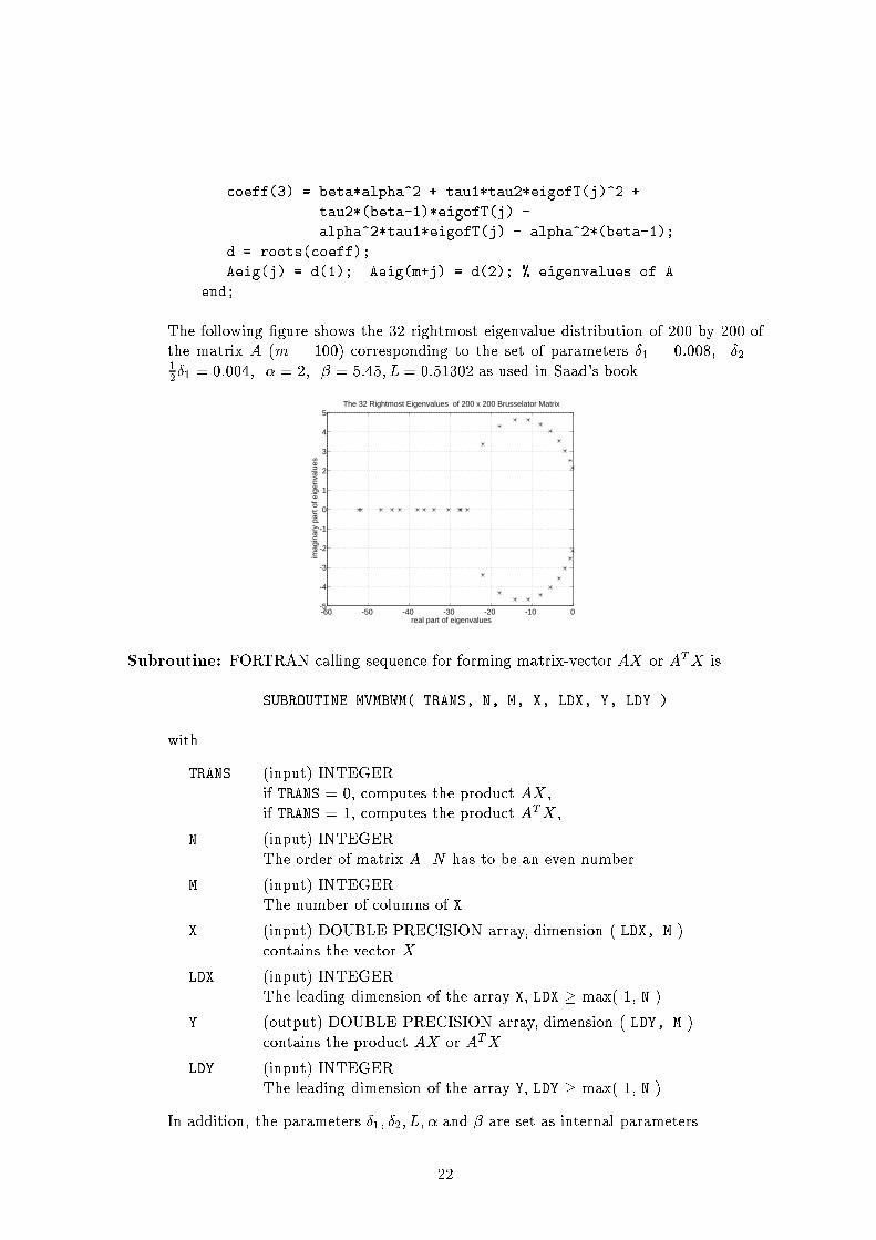
coeff(3) = beta*alpha^2 + tau1*tau2*eigofT(j)^2 + ...tau2*(beta-1)*eigofT(j) - ...alpha^2*tau1*eigofT(j) - alpha^2*(beta-1);d = roots(coeff);Aeig(j) = d(1); Aeig(m+j) = d(2); % eigenvalues of Aend;The following �gure shows the 32 rightmost eigenvalue distribution of 200 by 200 ofthe matrix A (m = 100) corresponding to the set of parameters �1 = 0:008; �2 =12�1 = 0:004; � = 2; � = 5:45; L= 0:51302 as used in Saad's book.-60 -50 -40 -30 -20 -10 0-5

-4

-3

-2

-1

0

1

2

3

4

5

real part of eigenvalues

imag

inar

y pa

rt o

f eig

enva

lues

The 32 Rightmost Eigenvalues of 200 x 200 Brusselator Matrix

Subroutine: FORTRAN calling sequence for forming matrix-vector AX or ATX isSUBROUTINE MVMBWM( TRANS, N, M, X, LDX, Y, LDY )withTRANS (input) INTEGERif TRANS = 0, computes the product AX ,if TRANS = 1, computes the product ATX ,N (input) INTEGERThe order of matrix A. N has to be an even number.M (input) INTEGERThe number of columns of X.X (input) DOUBLE PRECISION array, dimension ( LDX, M )contains the vector X .LDX (input) INTEGERThe leading dimension of the array X, LDX � max( 1, N ).Y (output) DOUBLE PRECISION array, dimension ( LDY, M )contains the product AX or ATX .LDY (input) INTEGERThe leading dimension of the array Y, LDY � max( 1, N ).In addition, the parameters �1; �2; L; � and � are set as internal parameters.22

Data �les: Filename/Key Order Number of nonzeros Data typeBW200 200 796 realBW2000 2000 7996 realReferences:P. Raschman, M. Kubicek and M. Maros, Waves in distributed chemical systems: ex-periments and computations, P. J. Holmes ed., New Approaches to Nonlinear Prob-lems in Dynamics - Proceedings of the Asilomar Conference Ground, Paci�c Grove,California 1979. The Engineering Foundation, SIAM, pp.271{288, 1980.Y. Saad, Numerical Methods for Large Eigenvalue Problems, Halsted Press, Div. ofJohn Wiley & Sons, Inc., New York, 1992

23

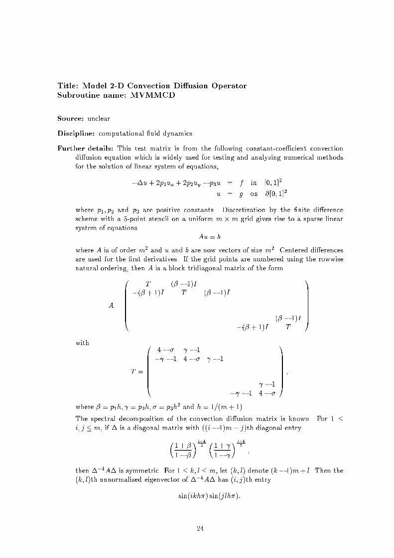
Title: Model 2-D Convection Di�usion OperatorSubroutine name: MVMMCDSource: unclearDiscipline: computational uid dynamicsFurther details: This test matrix is from the following constant-coe�cient convectiondi�usion equation which is widely used for testing and analyzing numerical methodsfor the solution of linear system of equations,��u+ 2p1ux + 2p2uy � p3u = f in [0; 1]2u = g on @[0; 1]2where p1; p2 and p3 are positive constants. Discretization by the �nite di�erencescheme with a 5-point stencil on a uniform m �m grid gives rise to a sparse linearsystem of equations Au = bwhere A is of order m2 and u and b are now vectors of size m2. Centered di�erencesare used for the �rst derivatives. If the grid points are numbered using the rowwisenatural ordering, then A is a block tridiagonal matrix of the formA = 0BBBBBBB@ T (� � 1)I�(� + 1)I T (� � 1)I. . . . . . . . .. . . . . . (� � 1)I�(� + 1)I T 1CCCCCCCAwith T = 0BBBBBBB@ 4� � � 1� � 1 4� � � 1. .. . . . . . .. . . . . . � 1� � 1 4� � 1CCCCCCCA ;where � = p1h; = p2h; � = p3h2 and h = 1=(m+ 1).The spectral decomposition of the convection di�usion matrix is known. For 1 �i; j � m, if � is a diagonal matrix with ((i� 1)m+ j)th diagonal entry�1 + �1� �� i�12 �1 + 1� � j�12 ;then ��1A� is symmetric. For 1 � k; l � m, let (k; l) denote (k� 1)m+ l. Then the(k; l)th unnormalized eigenvector of ��1A� has (i; j)th entrysin(ikh�) sin(jlh�):24

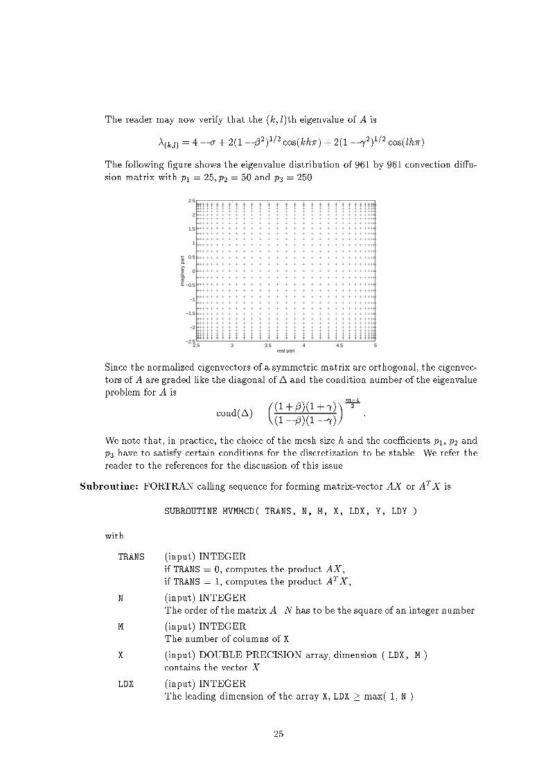
The reader may now verify that the (k; l)th eigenvalue of A is�(k;l) = 4� � + 2(1� �2)1=2 cos(kh�) + 2(1� 2)1=2 cos(lh�)The following �gure shows the eigenvalue distribution of 961 by 961 convection di�u-sion matrix with p1 = 25; p2 = 50 and p3 = 250.2.5 3 3.5 4 4.5 5

−2.5

−2

−1.5

−1

−0.5

0

0.5

1

1.5

2

2.5

real part

imag

inar

y pa

rt

Since the normalized eigenvectors of a symmetric matrix are orthogonal, the eigenvec-tors of A are graded like the diagonal of � and the condition number of the eigenvalueproblem for A is cond(�) = �(1 + �)(1 + )(1� �)(1� )�m�12 :We note that, in practice, the choice of the mesh size h and the coe�cients p1, p2 andp3 have to satisfy certain conditions for the discretization to be stable. We refer thereader to the references for the discussion of this issue.Subroutine: FORTRAN calling sequence for forming matrix-vector AX or ATX isSUBROUTINE MVMMCD( TRANS, N, M, X, LDX, Y, LDY )withTRANS (input) INTEGERif TRANS = 0, computes the product AX ,if TRANS = 1, computes the product ATX ,N (input) INTEGERThe order of the matrix A. N has to be the square of an integer number.M (input) INTEGERThe number of columns of X.X (input) DOUBLE PRECISION array, dimension ( LDX, M )contains the vector X .LDX (input) INTEGERThe leading dimension of the array X, LDX � max( 1, N ).25

Y (output) DOUBLE PRECISION array, dimension ( LDY, M )contains the product AX or ATX .LDY (input) INTEGERThe leading dimension of the array Y, LDY � max( 1, N ).In addition, p1, p2 and p3 are set as internal parameters.Data �les:Elman and Streit tested preconditioners for linear systems on six convection-di�usionmatrices arising on a 31 by 31 grid. Note that when p1 and p2 are large compared tothe grid size, the local error in the discretization is signi�cant. Also note that whenp1 and p2 are large the solution, u, forms boundary layers which are not practical toresolve using regular grids. The matrices correspond to the following choices of p1,p2and p3.Filename/Key Order Number of nonzeros Data type (p1; p2; p3)CDDE1 961 4681 real (1,2,30)CDDE2 961 4681 real (25,50,30)CDDE3 961 4681 real (1,2,80)CDDE4 961 4681 real (25,50,80)CDDE5 961 4681 real (1,2,250)CDDE6 961 4681 real (25,50,250)References:H. C. Elman and R. L Streit, Polynomial iteration for nonsymmetric inde�nite linearsystems, Lec. Notes in Math. Vol. 1230, J. P. Hennart, ed. Numerical AnalysisProceedings, Gauuajsato, Mexico, Springe Verlag, 1984.Y. Saad, Variations on Arnoldi's method for computing eigenelements of large unsym-metric matrices, Lin. Alg. Appl. 34:269{295, 1980.Z. Bai and G. W. Stewart, SRRIT { A FORTRAN subroutine to calculator the dom-inant invariant subspaces of a nonsymmetric matrix, Comp. Sci. Dept. Tech. Rep.TR-2908, Univ. of Maryland, MD, April 1992, (submitted to ACM TOMS).Z. Jia, Some numerical methods for large unsymmetric eigenproblems, Ph.D. thesis,The faculty of Mathematics, University of Bielefeld, Germany, Feb. 1994.R. B. Lehoucq, Analysis and implementation of an implicitly Restarted Arnoldi It-eration, Ph.D thesis, Department of Computational and Applied Methematics, RiceUniversity, TR95-13, May 1995.26

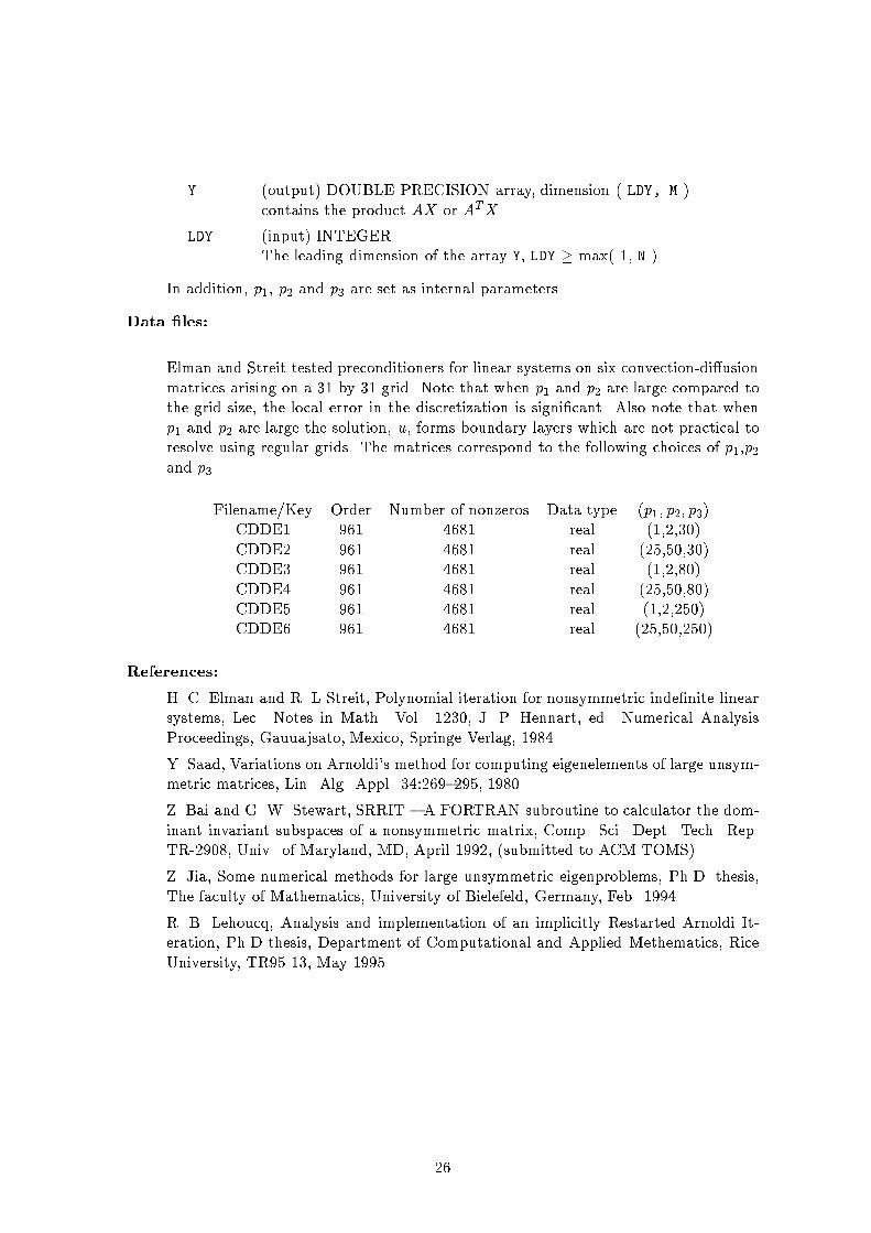
Title: Grcar MatrixSubroutine name: MVMGRCSource: J. Grcar, Sandia National Lab.Discipline: numerical linear algebraFurther details: An n� n Grcar matrix is a nonsymmetric Toeplitz matrix:A = 0BBBBBBBBBBBBB@ 1 1 1 1�1 1 1 1 1�1 1 1 1 1. . . . . . . . . . . . . . .�1 1 1 1 1�1 1 1 1�1 1 1�1 1 1CCCCCCCCCCCCCAThe matrix has sensitive eigenvalues. The following �gures are the eigenvalue distri-bution of 100 by 100 Grcar matrix A and AT , computed by QR algorithm in Matlab.0 0.2 0.4 0.6 0.8 1 1.2 1.4 1.6 1.8

−2.5

−2

−1.5

−1

−0.5

0

0.5

1

1.5

2

2.5

0 0.2 0.4 0.6 0.8 1 1.2 1.4 1.6 1.8−2.5

−2

−1.5

−1

−0.5

0

0.5

1

1.5

2

2.5

Subroutine: FORTRAN calling sequence for forming matrix-vector AX or ATX isSUBROUTINE MVMGRC( TRANS, N, M, X, LDX, Y, LDY )withTRANS (input) INTEGERif TRANS = 0, computes the product AX ,if TRANS = 1, computes the product ATX ,N (input) INTEGERThe order of the matrix A.M (input) INTEGERThe number of columns of X.X (input) DOUBLE PRECISION array, dimension ( LDX, M )contains the vector X . 27

LDX (input) INTEGERThe leading dimension of the array X, LDX � max( 1, N ).Y (output) DOUBLE PRECISION array, dimension ( LDY, M )contains the product AX or ATX .LDY (input) INTEGERThe leading dimension of the array Y, LDY � max( 1, N ).References:J. Grcar, Operator coe�cient methods for linear equations, Sandia National Lab.Rep. SAND89-8691, Nov. 1989.N.M. Nachtigal, L. Reichel and L.N. Trefethen, A hybrid GMRES algorithm for non-symmetric linear systems, SIAM J. Matrix Anal. Appl., 13 (1992), pp. 796-825.N. J. Higham, A collection of test matrices in MATLAB, ACM Trans. Math. Softw.17:289{305, 1991.

28

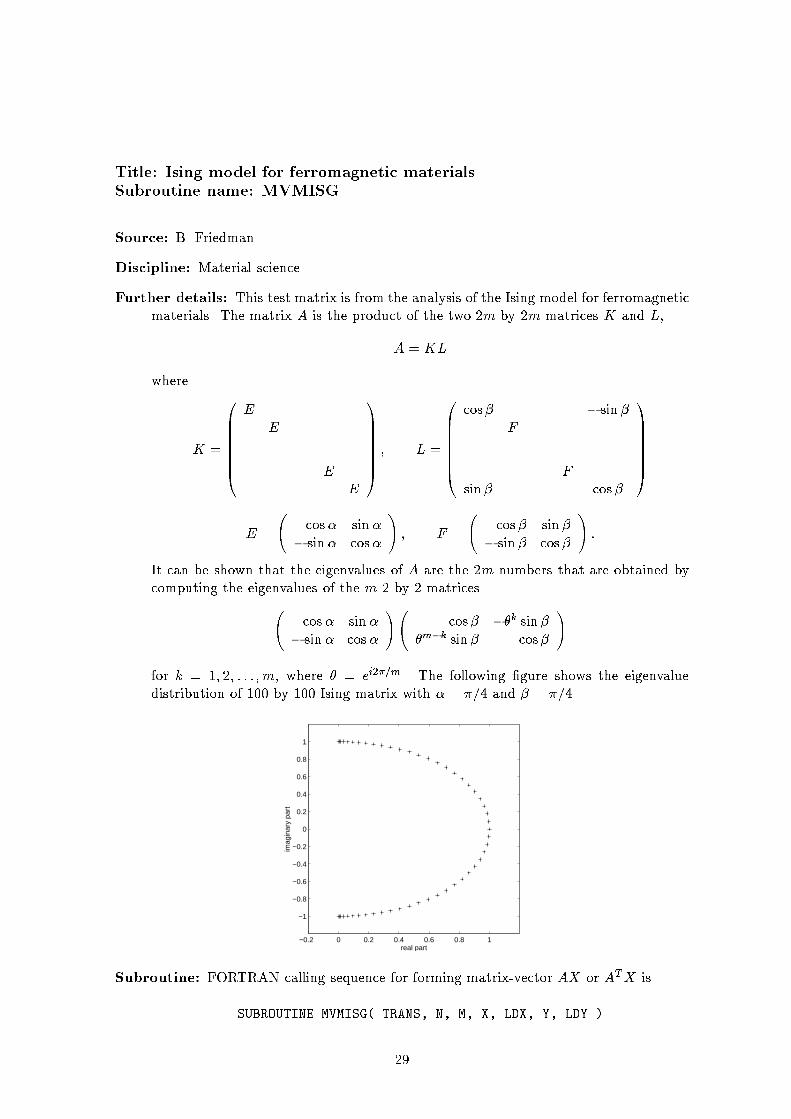
Title: Ising model for ferromagnetic materialsSubroutine name: MVMISGSource: B. FriedmanDiscipline: Material scienceFurther details: This test matrix is from the analysis of the Ising model for ferromagneticmaterials. The matrix A is the product of the two 2m by 2m matrices K and L,A = KLwhere K = 0BBBBBB@ E E . . . E E 1CCCCCCA ; L = 0BBBBBB@ cos� � sin �F . . . Fsin � cos � 1CCCCCCAE = cos� sin�� sin � cos� ! ; F = cos � sin �� sin � cos � ! :It can be shown that the eigenvalues of A are the 2m numbers that are obtained bycomputing the eigenvalues of the m 2 by 2 matrices cos� sin �� sin � cos� ! cos� ��k sin ��m�k sin � cos� !for k = 1; 2; : : : ; m, where � = ei2�=m. The following �gure shows the eigenvaluedistribution of 100 by 100 Ising matrix with � = �=4 and � = �=4−0.2 0 0.2 0.4 0.6 0.8 1

−1

−0.8

−0.6

−0.4

−0.2

0

0.2

0.4

0.6

0.8

1

real part

imag

inar

y pa

rt

Subroutine: FORTRAN calling sequence for forming matrix-vector AX or ATX isSUBROUTINE MVMISG( TRANS, N, M, X, LDX, Y, LDY )29

withTRANS (input) INTEGERif TRANS = 0, computes the product AX ,if TRANS = 1, computes the product ATX ,N (input) INTEGERThe order of the matrix A. N has to be an even number.M (input) INTEGERThe number of columns of X.X (input) DOUBLE PRECISION array, dimension ( LDX, M )contains the vector X .LDX (input) INTEGERThe leading dimension of the array X, LDX � max( 1, N ).Y (output) DOUBLE PRECISION array, dimension ( LDY, M )contains the product AX or ATX .LDY (input) INTEGERThe leading dimension of the array Y, LDY � max( 1, N ).In addition, � and � are set as internal parameters.References:B. Kaufman, Crystal statistics II, Phys. Rev. 76, pp.1232, 1949.B. Friedman, Eigenvalues of Composite matrices, Proc. Cambridge Philos. Soc. 57,pp.37-49, 1961M. Marcus and H. Minc, A survey of Matrix Theory and matrix inequalities, Doveredition, New York, 1992.Afternotes:This Ising model was proposed to explain properties of ferromagnets but since thenit has found application to topics in chemistry and biology as well as physics. Forany reader unfamiliar with the model an excellent introduction is [B. A. Cipra, AnIntroduction to the Ising Model, American Mathematical Monthly, 94:937{959, 1987].A numerical method for approximating the leading eigenvalues of 2D Ising modelsusing a transfer matrix of order 2n with n = 30 is reported in [B. Parlett and W.Heng, The Method of Minimal Representations in 2D Ising Model Calculations, J.Comp. Phy. 114, pp.257{264, 1994].We plan to include the transfer matrix in the future version of this collection.30

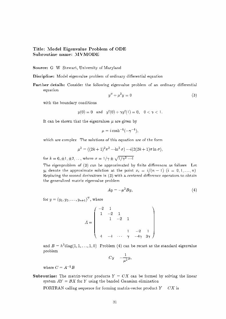
Title: Model Eigenvalue Problem of ODESubroutine name: MVMODESource: G. W. Stewart, University of MarylandDiscipline: Model eigenvalue problem of ordinary di�erential equation.Further details: Consider the following eigenvalue problem of an ordinary di�erentialequation y00 + �2y = 0 (3)with the boundary conditionsy(0) = 0 and y0(0) + y0(1) = 0; 0 < < 1:It can be shown that the eigenvalues � are given by� = i cosh�1(� �1);which are complex. The solutions of this equation are of the form�2 = ((2k+ 1)2�2 � ln2 �)� i(2(2k+ 1)� ln �);for k = 0;�1;�2; : : :, where � = 1= �p1= 2 � 1.The eigenproblem of (3) can be approximated by �nite di�erences as follows. Letyi denote the approximate solution at the point xi = i=(n + 1) (i = 0; 1; : : : ; n).Replacing the second derivatives in (3) with a centered di�erence operators to obtainthe generalized matrix eigenvalue problemAy = ��2By; (4)for y = (y1; y2; : : : ; yn+1)T, whereA = 0BBBBBBBB@ �2 11 �2 11 �2 1.. . . . . . . .1 �2 14 �1 � � � �4 3 1CCCCCCCCAand B = h2diag(1; 1; : : : ; 1; 0). Problem (4) can be recast as the standard eigenvalueproblem Cy = � 1�2 y;where C = A�1B.Subroutine: The matrix-vector products Y = CX can be formed by solving the linearsystem AY = BX for Y using the banded Gaussian elimination.FORTRAN calling sequence for forming matrix-vector product Y = CX is31

SUBROUTINE MVMODE( N, M, X, LDX, Y, LDY )withN (input) INTEGERThe order of the matrix C.M (input) INTEGERThe number of columns of X.X (input) DOUBLE PRECISION array, dimension ( LDX, M )contains the vector X .LDX (input) INTEGERThe leading dimension of the array X, LDX � max( 1, N ).Y (output) DOUBLE PRECISION array, dimension ( LDY, M )contains the product CX .LDY (input) INTEGERThe leading dimension of the array Y, LDY � max( 1, N ).In addition, is set as an internal parameters.2N workspace is required for the banded Gaussian elimination. As a default value,3*2001 workspace is set internally. As a result, N should be less and equal to 2001.Otherwise, user should set a larger workspace.Data �les: In the data �les, = 1=100.Filename/Key Order Number of nonzeros Data typeODEP400A 400 1201 realODEP400B 400 399 realReferences:G. W. Stewart, SRRIT { A FORTRAN subroutine to calculator the dominant invari-ant subspaces of a real matrix, Comp. Sci. Dept. Tech. Rep. TR-514, Univ. ofMaryland, College Park, Nov. 1978.Z. Bai and G. W. Stewart, SRRIT { A FORTRAN subroutine to calculator the dom-inant invariant subspaces of a nonsymmetric matrix, Comp. Sci. Dept. Tech. Rep.TR-2908, Univ. of Maryland, MD, April 1992, (submitted to ACM TOMS).32

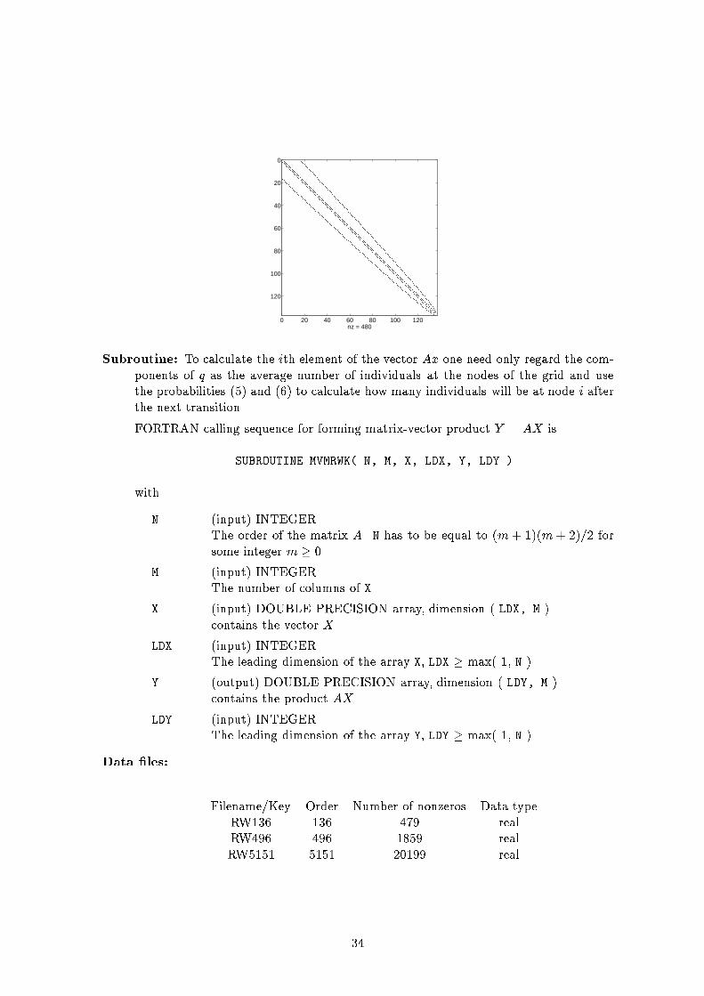
Title: Markov Chain Transition MatrixSubroutine name: MVMRWKSource: G. W. Stewart, University of MarylandDiscipline: Probability theory and its applicationsFurther details: Consider a random walk on an (m+1)�(m+1) triangular grid, illustratedbelow for m = 6. 6 �5 � �4 � � �3 � � � �2 � � � � �1 � � � � � �0 � � � � � � �j=i 0 1 2 3 4 5 6The points of the grid are labeled (j; i); (i= 0; : : : ; m; j = 0; : : : ; m�i): From the point(j; i), a transition may take place to one of the four adjacent points (j + 1; i); (j; i+1); (j � 1; i); (j; i� 1). The probability of jumping to either of the nodes (j � 1; i) or(j; i� 1) is pd(j; i) = j + im (5)with the probability being split equally between the two nodes when both nodes areon the grid. The probability of jumping to either of the nodes (j+ 1; i) or (j; i+ 1) ispu(j; i) = 1� pd(j; i): (6)with the probability again being split when both nodes are on the grid.If the (m+ 1)(m+ 2)=2 nodes (j; i) are numbered 1; 2; : : : ; (m+ 1)(m+ 2)=2 in somefashion, then the random walk can be expressed as a �nite Markov chain with tran-sition matrix A of order n = (m + 1)(m+ 2)=2 consisting of the probabilities akl ofjumping from node l to node k (A is actually the transpose of the usual transitionmatrix; see [Feller]).We are primarily interested in the steady state probabilities of the chain, which isordinarily the appropriately scaled eigenvector corresponding to the eigenvalue unity.The following plot shows the sparsity pattern of the resulted random walk matrix oforder 136 (i.e. m = 15).33

0 20 40 60 80 100 120

0

20

40

60

80

100

120

nz = 480Subroutine: To calculate the ith element of the vector Ax one need only regard the com-ponents of q as the average number of individuals at the nodes of the grid and usethe probabilities (5) and (6) to calculate how many individuals will be at node i afterthe next transition.FORTRAN calling sequence for forming matrix-vector product Y = AX isSUBROUTINE MVMRWK( N, M, X, LDX, Y, LDY )withN (input) INTEGERThe order of the matrix A. N has to be equal to (m+ 1)(m+ 2)=2 forsome integer m � 0.M (input) INTEGERThe number of columns of X.X (input) DOUBLE PRECISION array, dimension ( LDX, M )contains the vector X .LDX (input) INTEGERThe leading dimension of the array X, LDX � max( 1, N ).Y (output) DOUBLE PRECISION array, dimension ( LDY, M )contains the product AX .LDY (input) INTEGERThe leading dimension of the array Y, LDY � max( 1, N ).Data �les: Filename/Key Order Number of nonzeros Data typeRW136 136 479 realRW496 496 1859 realRW5151 5151 20199 real34

References:W. Feller, An introduction to probability theory and its applications, John Wiley,New York, 1961G. W. Stewart, SRRIT { A FORTRAN subroutine to calculator the dominant invari-ant subspaces of a real matrix, Comp. Sci. Dept. Tech. Rep. TR-514, Univ. ofMaryland, College Park, Nov. 1978.Y. Saad, Numerical methods for large eigenvalue problems. Halsted Press, Div. ofJohn Wiley & Sons, Inc., New York, 1992.I. S. Du� and J. A. Scott, Computing selected eigenvalues of sparse unsymmetricmatrices using subspace iteration, ACM TOMS 19:137-159, 1993Z. Bai and G. W. Stewart, SRRIT { A FORTRAN subroutine to calculator the dom-inant invariant subspaces of a nonsymmetric matrix, Comp. Sci. Dept. Tech. Rep.TR-2908, Univ. of Maryland, MD, April 1992 (submitted to ACM TOMS).

35

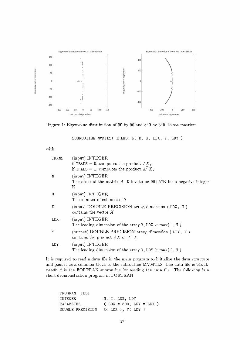
Title: Tolosa MatrixSubroutine name: MVMTLSSource: S. Godet-Thobie, CERFACS and C. B�es, Aerospatiale, FranceDiscipline: AeroelasticityFuture details: The Tolosa matrix arises in the stability analysis of a model of an airplanein ight. The interesting modes of this system are described by complex eigenvalueswhose imaginary parts lie in a prescribed frequency range. The task is to compute theeigenvalues with largest imaginary parts. The problem has been analyzed at CER-FACS (Centre Europeen de Recherche et de Formation Avancee en Calcul Scienti�que)in cooperation with the Aerospatiale Aircraft Division3.The matrix is a sparse 5� 5 block matrix of order n = 90+5k for an integer k >= 0.When n = 90, each block is of dimension 18� 18 andA = 0BBBBB@ 0 I 0 0 0X1 X2 X3 X4 X50 I L1 0 00 I 0 L2 00 I 0 0 L3 1CCCCCAwhere Li = �iI , i = 1; 2; 3, and Xi and �i are given data. When n > 90,A = 0BBBBB@ 0 I 0 0 0Y1 Y2 Y3 Y4 Y50 I L1 0 00 I 0 L2 00 I 0 0 L3 1CCCCCAwhere Y1 = X1 00 diag(xi) ! ; xi = �!2i ; i = 1; : : : ; m� 18;Y2 = X2 00 diag(yi) ! ; yi = �2�i!i; i = 1; : : : ; m� 18;Yi = Xi 00 0 ! ; i = 3; 4; 5;and !i = 150 + 6i; �i = c1i+ c2; c1 = :299n=5� 18 ; c2 = 0:001� c1:The following fugures show the eigenvalue distribution of Tolosa matrices of orders 90and 340.Subroutine: FORTRAN calling sequence for forming matrix-vector AX or ATX is3Tolosa is the latin name of Toulouse, France, the location of CERFACS.36

-150

-100

-50

0

50

100

150

-150 -100 -50 0 50 100 150

*

*

*

*

*

*

*

*

*

*

*

*

*

*

*

*

*

*

*

*

*

*

*

*

*

*

*

*

*

*

*

*

*

*

*

*

* ****************** ***************** ******************

real part of eigenvalues

imag

inar

y pa

rt o

f ei

genv

alue

s

Eigenvalue Distribution of 90 x 90 Tolosa Matrix

-400

-200

0

200

400

-400 -200 0 200 400

******************************************************************************************************************************************************

*

*

*

*

*

*

*

*

*

*

*

*

*

*

*

*

*

*

*

*

*

*

*

*

*

*

*

*

*

*

*

*

*

*

*

*

*

*

*

*

*

*

*

*

*

*

*

*

*

*

*

*

*

*

*

*

*

*

*

*

*

*

*

*

*

*

*

*

*

*

*

*

*

*

*

*

*

*

*

*

*

*

*

*

*

*

*

*

*

*

*

*

*

*

*

*

*

*

*

*

*

*

*

*

*

*

*

*

*

*

*

*

*

*

*

*

*

*

*

*

*

*

*

*

*

*

*

*

*

*

*

*

**********************************************************

real part of eigenvalues

imag

inar

y pa

rt o

f ei

genv

alue

s

Eigenvalue Distribution of 340 x 340 Tolosa Matrix

Figure 1: Eigenvalue distribution of 90 by 90 and 340 by 340 Tolosa matricesSUBROUTINE MVMTLS( TRANS, N, M, X, LDX, Y, LDY )withTRANS (input) INTEGERif TRANS = 0, computes the product AX ,if TRANS = 1, computes the product ATX ,N (input) INTEGERThe order of the matrix A. N has to be 90+5*K for a negative integerK.M (input) INTEGERThe number of columns of X.X (input) DOUBLE PRECISION array, dimension ( LDX, M )contains the vector X .LDX (input) INTEGERThe leading dimension of the array X, LDX � max( 1, N ).Y (output) DOUBLE PRECISION array, dimension ( LDY, M )contains the product AX or ATX .LDY (input) INTEGERThe leading dimension of the array Y, LDY � max( 1, N ).It is required to read a data �le in the main program to initialize the data structureand pass it as a common block to the subroutine MVMTLS. The data �le is block.readb.f is the FORTRAN subroutine for reading the data �le. The following is ashort deomonstration program in FORTRAN.. PROGRAM TESTINTEGER N, I, LDX, LDYPARAMETER ( LDX = 500, LDY = LDX )DOUBLE PRECISION X( LDX ), Y( LDY )37

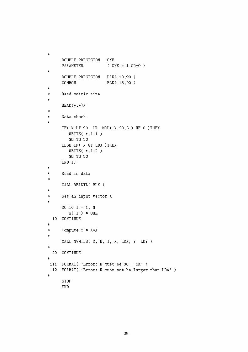
* DOUBLE PRECISION ONEPARAMETER ( ONE = 1.0D+0 )* DOUBLE PRECISION BLK( 18,90 )COMMON BLK( 18,90 )** Read matrix size* READ(*,*)N** Data check* IF( N.LT.90 .OR. MOD( N-90,5 ).NE.0 )THENWRITE( *,111 )GO TO 20ELSE IF( N.GT.LDX )THENWRITE( *,112 )GO TO 20END IF** Read in data* CALL READTL( BLK )** Set an input vector X* DO 10 I = 1, NX( I ) = ONE10 CONTINUE** Compute Y = A*X* CALL MVMTLS( 0, N, 1, X, LDX, Y, LDY )* 20 CONTINUE*111 FORMAT( 'Error: N must be 90 + 5K' )112 FORMAT( 'Error: N must not be larger than LDA' )* STOPEND 38

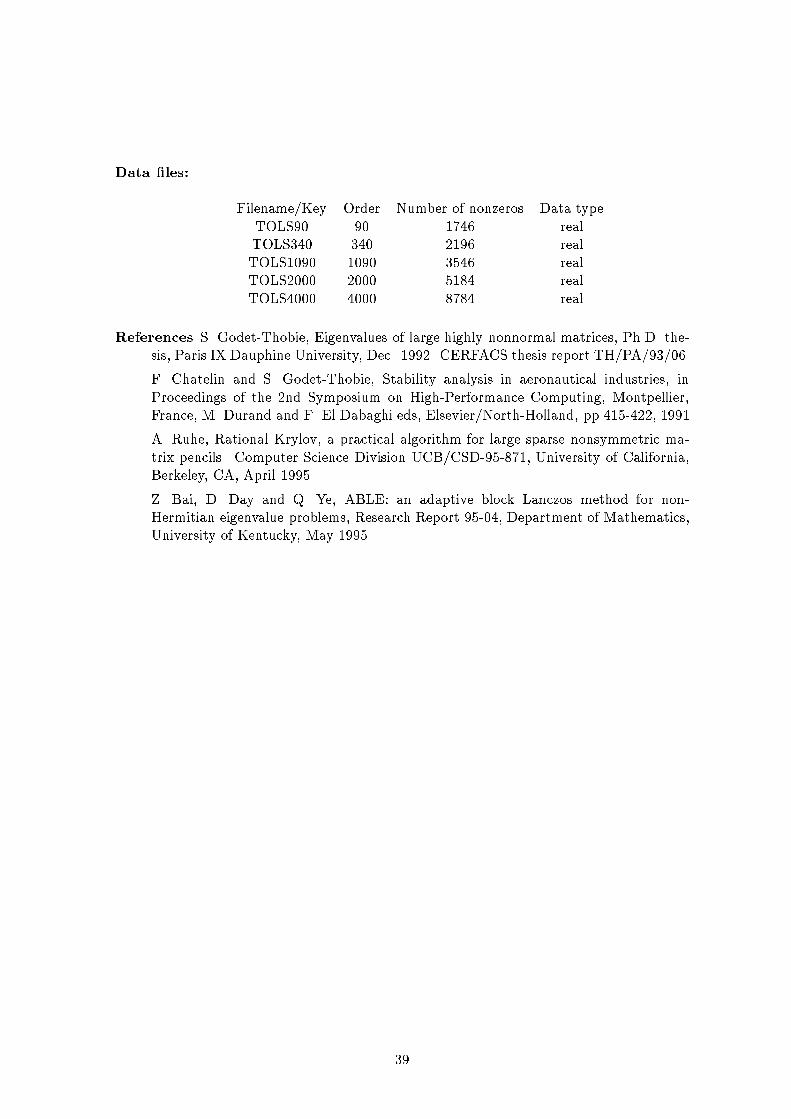
Data �les: Filename/Key Order Number of nonzeros Data typeTOLS90 90 1746 realTOLS340 340 2196 realTOLS1090 1090 3546 realTOLS2000 2000 5184 realTOLS4000 4000 8784 realReferences S. Godet-Thobie, Eigenvalues of large highly nonnormal matrices, Ph.D. the-sis, Paris IX Dauphine University, Dec. 1992. CERFACS thesis report TH/PA/93/06.F. Chatelin and S. Godet-Thobie, Stability analysis in aeronautical industries, inProceedings of the 2nd Symposium on High-Performance Computing, Montpellier,France, M. Durand and F. El Dabaghi eds, Elsevier/North-Holland, pp.415-422, 1991A. Ruhe, Rational Krylov, a practical algorithm for large sparse nonsymmetric ma-trix pencils. Computer Science Division UCB/CSD-95-871, University of California,Berkeley, CA, April 1995.Z. Bai, D. Day and Q. Ye, ABLE: an adaptive block Lanczos method for non-Hermitian eigenvalue problems, Research Report 95-04, Department of Mathematics,University of Kentucky, May 1995

39

Appendix CMatrices in Subroutine FormatTitle Subroutine NamesRandom Sparse Matrix MATRANModel elliptic Partial Di�erential Equation MATPDE

40

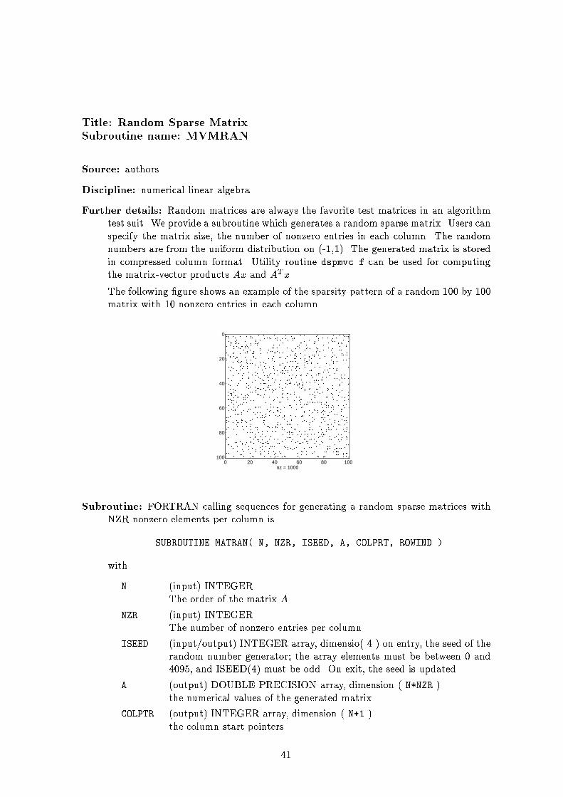
Title: Random Sparse MatrixSubroutine name: MVMRANSource: authorsDiscipline: numerical linear algebraFurther details: Random matrices are always the favorite test matrices in an algorithmtest suit. We provide a subroutine which generates a random sparse matrix. Users canspecify the matrix size, the number of nonzero entries in each column. The randomnumbers are from the uniform distribution on (-1,1). The generated matrix is storedin compressed column format. Utility routine dspmvc.f can be used for computingthe matrix-vector products Ax and ATx.The following �gure shows an example of the sparsity pattern of a random 100 by 100matrix with 10 nonzero entries in each column.0 20 40 60 80 100

0

20

40

60

80

100

nz = 1000Subroutine: FORTRAN calling sequences for generating a random sparse matrices withNZR nonzero elements per column isSUBROUTINE MATRAN( N, NZR, ISEED, A, COLPRT, ROWIND )withN (input) INTEGERThe order of the matrix A.NZR (input) INTEGERThe number of nonzero entries per column.ISEED (input/output) INTEGER array, dimensio( 4 ) on entry, the seed of therandom number generator; the array elements must be between 0 and4095, and ISEED(4) must be odd. On exit, the seed is updated.A (output) DOUBLE PRECISION array, dimension ( N*NZR )the numerical values of the generated matrix.COLPTR (output) INTEGER array, dimension ( N+1 )the column start pointers.41

ROWIND (output) INTEGER array, dimension ( N*NZR )The row indices.References:LAPACK random number generator DLARAN is used to generate random numbers.

42

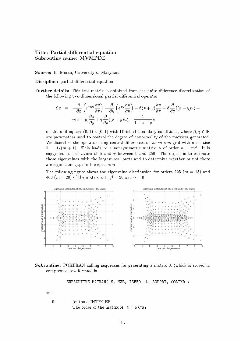
Title: Partial di�erential equationSubroutine name: MVMPDESource: H. Elman, University of MarylandDiscipline: partial di�erential equationFurther details: This test matrix is obtained from the �nite di�erence discretization ofthe following two-dimensional partial di�erential operatorLu = � @@x �e�xy @u@x�� @@y �exy @u@y�+ �(x+ y)@u@x + � @@x((x+ y)u) + (x+ y)@u@y + @@y ((x+ y)u) + 11 + x+ yuon the unit square (0; 1)� (0; 1) with Dirichlet boundary conditions, where �; 2 IRare parameters used to control the degree of nonormality of the matrices generated.We discretize the operator using central di�erences on an m�m grid with mesh sizeh = 1=(m + 1). This leads to a nonsymmetric matrix A of order n = m2. It issuggested to use values of � and between 0 and 250. The object is to estimatethose eigenvalues with the largest real parts and to determine whether or not thereare signi�cant gaps in the spectrum.The following �gure shows the eigenvalue distribution for orders 225 (m = 15) and400 (m = 20) of the matrix with � = 20 and = 0.0 1 2 3 4 5 6 7 8 9

-4

-3

-2

-1

0

1

2

3

4

real part of eigenvalues

imag

inar

y pa

rt o

f eig

enva

lues

Eigenvalue Distribution of 225 x 225 Model PDE Matrix

0 1 2 3 4 5 6 7 8 9-3

-2

-1

0

1

2

3

real part of eigenvalues

imag

inar

y pa

rt o

f eig

enva

lues

Eigenvalue Distribution of 400 x 400 Model PDE Matrix

Subroutine: FORTRAN calling sequences for generating a matrix A (which is stored incompressed row format) isSUBROUTINE MATRAN( N, NZR, ISEED, A, ROWPRT, COLIND )withN (output) INTEGERThe order of the matrix A. N = NX*NY.43

NX (input) INTEGERThe number of mesh points in the X-axisNY (input) INTEGERThe number of mesh points in the Y-axisA (output) DOUBLE PRECISION array, dimension ( NZ )the numerical values of the generated matrix, where the number ofnonzero elements NZ = NX*NY + (NX-1)*NY*2 + NX*(NY-1)*2.ROWPTR (output) INTEGER array, dimension ( N+1 )the row start pointers.COLIND (output) INTEGER array, dimension ( N*NZR )The column indices.RHS (output) DOUBLE PRECISION array, dimension ( N )The right hand side of the linear system of equation Ax = f .In addition, � and are set as internal parameters, which may be altered.The utility routine dspmvr.f can be used for computing the matrix-vector productsAx and ATx.Data �les: Filename/Key Order Number of nonzeros Data typePDE225 225 1065 realPDE900 900 4380 realPDE2961 2961 14585 realReferences:H. Elman, Iterative Methods for Large Sparse Nonsymmetric Systems of Linear Equa-tions. PhD thesis, Yale University, New Haven, CT, 1982.J. Cullum and R. A. Willoughby, A Practical Procedure for Computing Eigenvalues ofLarge Sparse Nonsymmetric Matrices, In Large Scale Eigenvalue Problem, J. Cullumand R. A. Willoughby eds. Elsevier Science Pub. North-Holland, 1986.R. W. Freund, M. H. Gutknecht, and N. M. Nachtigal. An implementation of thelook-ahead Lanczos algorithm for non-Hermitian matrices. SIAM J. Sci. Comput.,14:137{158, 1993.44

Appendix C: List of Utility Routinesdprtmt.f FORTRAN subroutine for writing a real sparse matrix in the standard HBsparse format. It is assumed that the matrix is stored in the compressedcolumn format.zprtmt.f complex version of dprtmt.f .dreadm.f FORTRAN subroutine for reading a real sparse matrix which is in standardHB sparse format.zreadm.f complex version of dreadm.f .dreadhb.c C subroutine for reading a real sparse matrix which is in standard HB sparseformat.dm2hb.m Matlab M-�le for writing a real sparse matrix in the standard HB sparseformat.zm2hb.m complex version of dm2hb.m .dspmvc.f FORTRAN subroutine for computing the matrix-vector product Ax or ATx,it is assumed that A is stored in compressed column format.zspmvc.f complex version of dspmvc.f.dspmvr.f FORTRAN subroutine for computing the matrix-vector product Ax or ATx,it is assumed that A is stored in compressed row format.zspmvr.f complex version of dspmvr.f.mvm2hb.f FORTRAN program to illustrate that if one has a matrix-vector productsubroutine, how to write it in the standard HB sparse matrix format.In addition, �le hb2matlabinfo provides information how to get software from MathWorkto read a HB sparse matrix format into Matlab.45