Embed Size (px)
Citation preview
Collateralized Debt Obligations: Structuring, Pricing and Risk Analysis
Mark DavisImperial College London
and
Hanover Square Capital
Institute of Actuaries, 19 March 2003

Agenda
Overview• Motivation• Structure• Risk Engineering
Cash Flow• Waterfall structure• Cash flow vs. Synthetic• Funded vs. unfunded
Default risk analysis• Moodys diversity scores• Bionomial expansion technique• Dynamic models
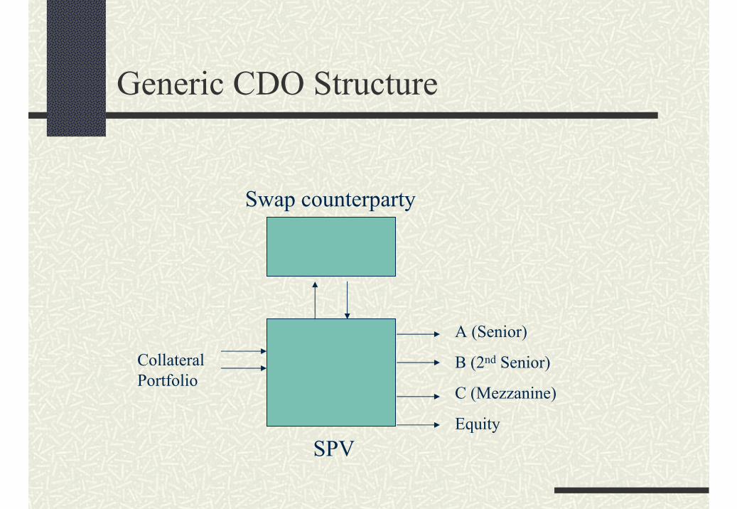
Generic CDO Structure
A (Senior)
B (2nd Senior)
C (Mezzanine)
Equity
CollateralPortfolio
Swap counterparty
SPV
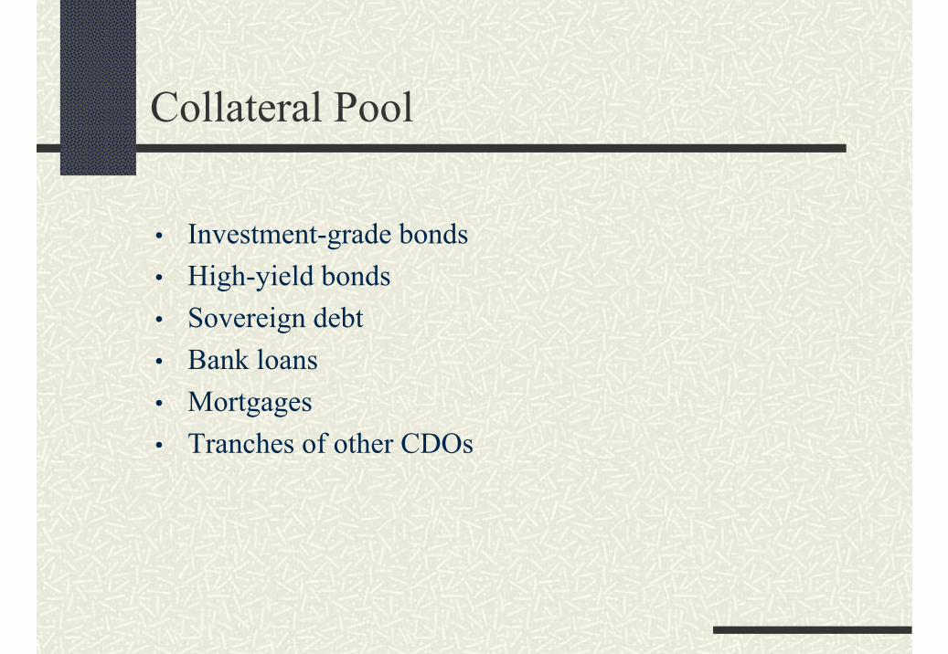
Collateral Pool
• Investment-grade bonds• High-yield bonds• Sovereign debt• Bank loans• Mortgages• Tranches of other CDOs
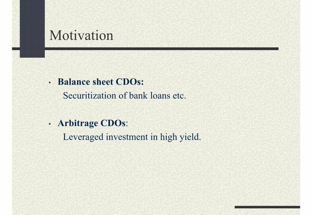
Motivation
• Balance sheet CDOs:Securitization of bank loans etc.
• Arbitrage CDOs:Leveraged investment in high yield.
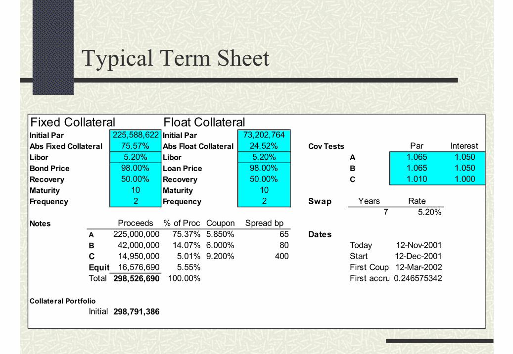
Typical Term Sheet
Fixed Collateral Float CollateralInitial Par 225,588,622 Initial Par 73,202,764Abs Fixed Collateral 75.57% Abs Float Collateral 24.52% Cov Tests Par InterestLibor 5.20% Libor 5.20% A 1.065 1.050Bond Price 98.00% Loan Price 98.00% B 1.065 1.050Recovery 50.00% Recovery 50.00% C 1.010 1.000Maturity 10 Maturity 10Frequency 2 Frequency 2 Swap Years Rate
7 5.20%Notes Proceeds % of Proc Coupon Spread bp
A 225,000,000 75.37% 5.850% 65 DatesB 42,000,000 14.07% 6.000% 80 Today 12-Nov-2001C 14,950,000 5.01% 9.200% 400 Start 12-Dec-2001Equit 16,576,690 5.55% First Coupo 12-Mar-2002Total 298,526,690 100.00% First accru 0.246575342
Collateral PortfolioInitial 298,791,386
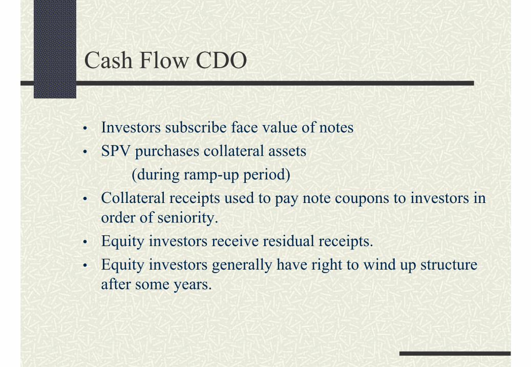
Cash Flow CDO
• Investors subscribe face value of notes• SPV purchases collateral assets
(during ramp-up period)• Collateral receipts used to pay note coupons to investors in
order of seniority.• Equity investors receive residual receipts.• Equity investors generally have right to wind up structure
after some years.
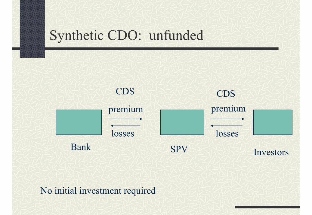
Synthetic CDO: unfunded
premium
lossesBank
premium
losses
InvestorsSPV
No initial investment required
CDS CDS
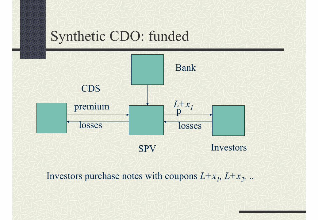
Synthetic CDO: funded
premium
lossesplosses
Bank
SPV
Investors purchase notes with coupons L+x1, L+x2, ..
L+x1
CDS
Investors

Waterfall structure
FeesSwap paymentsClass A interestMaturing collateral redeems class A notes, then class B ..Further redemption of class A notes to meet coverage testsClass B interest……Subordinate fees to collateral managerResidual receipts to equity note holders
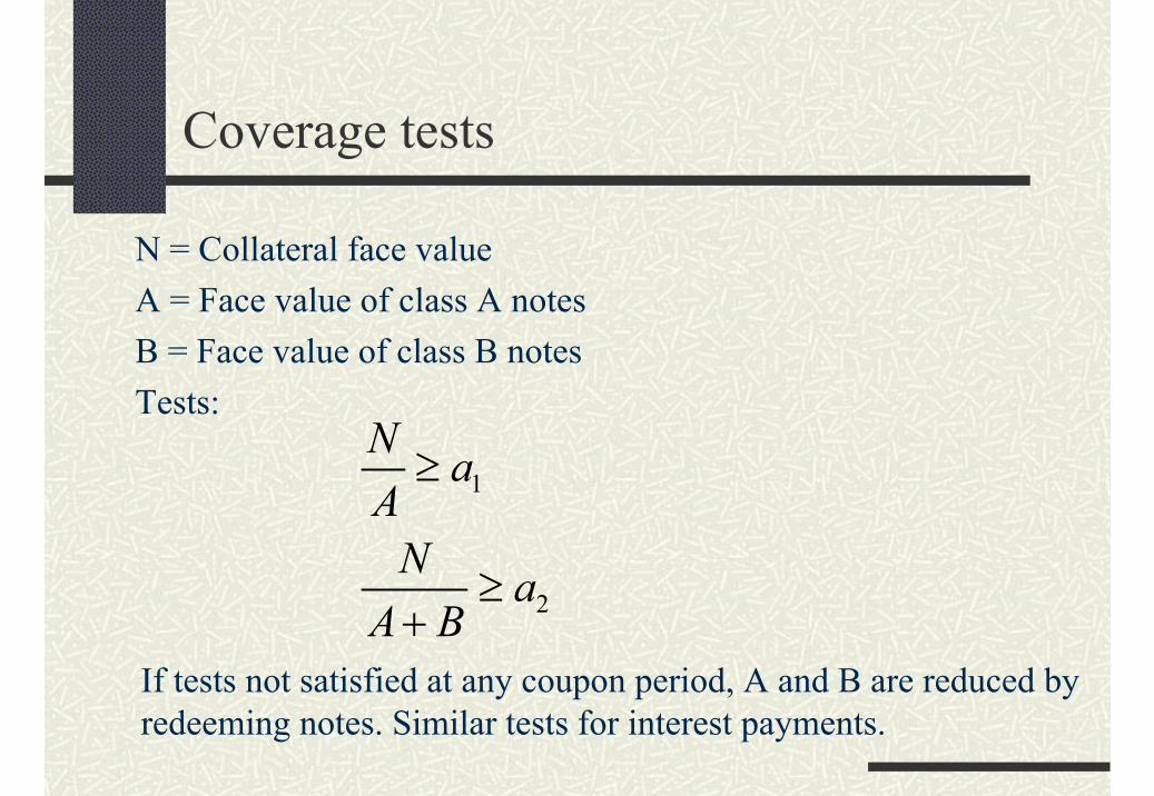
Coverage tests
N = Collateral face valueA = Face value of class A notesB = Face value of class B notesTests:
1
2
N aA
N aA B
≥
≥+
If tests not satisfied at any coupon period, A and B are reduced by redeeming notes. Similar tests for interest payments.
Default and Recovery
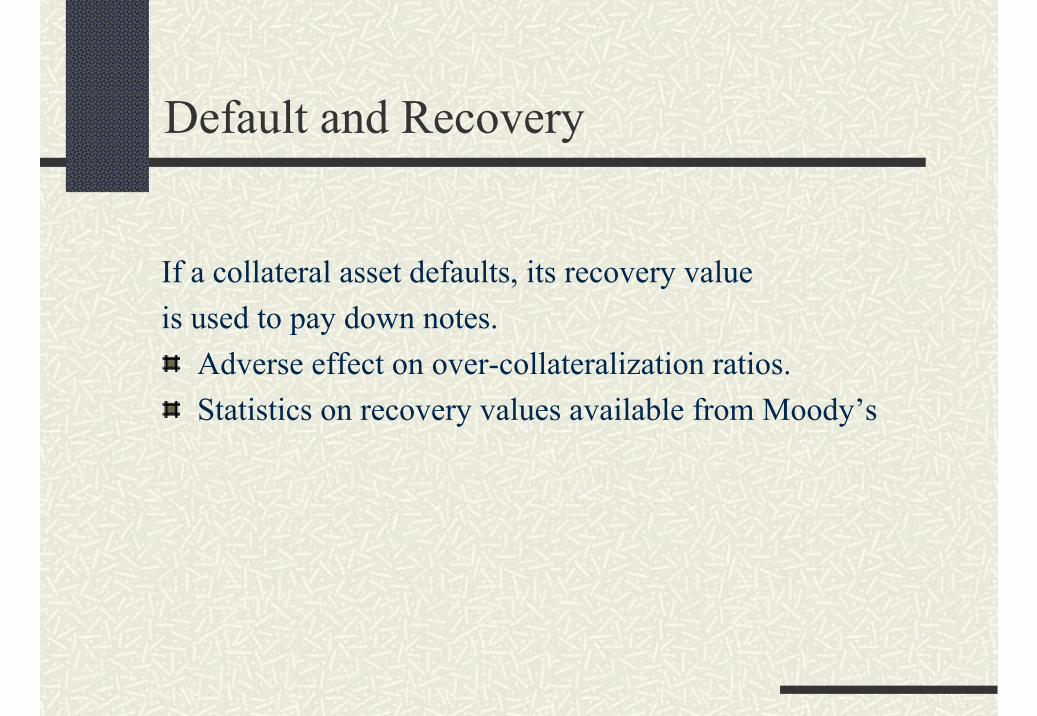
If a collateral asset defaults, its recovery valueis used to pay down notes.
Adverse effect on over-collateralization ratios. Statistics on recovery values available from Moody’s
Interest rate swap
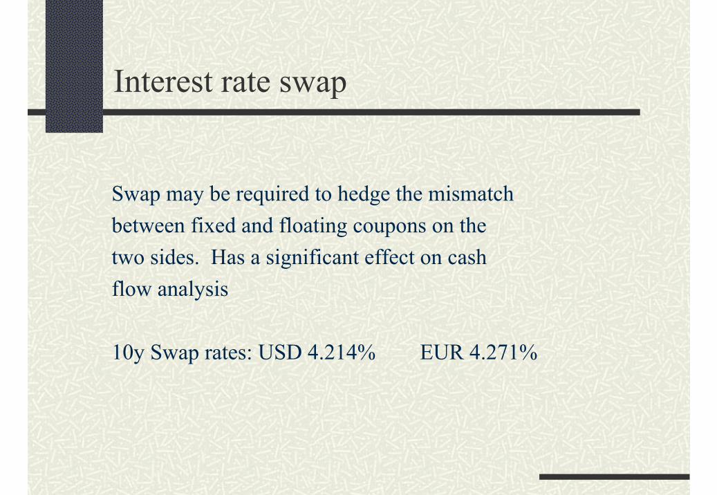
Swap may be required to hedge the mismatchbetween fixed and floating coupons on the two sides. Has a significant effect on cashflow analysis
10y Swap rates: USD 4.214% EUR 4.271%
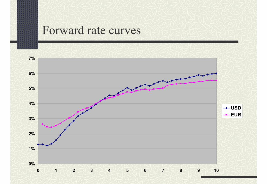
Forward rate curves
0%
1%
2%
3%
4%
5%
6%
7%
0 1 2 3 4 5 6 7 8 9 10
USDEUR
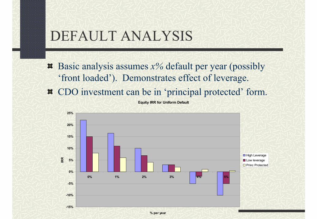
DEFAULT ANALYSIS
Basic analysis assumes x% default per year (possibly ‘front loaded’). Demonstrates effect of leverage. CDO investment can be in ‘principal protected’ form.
Equity IRR for Uniform Default
-15%
-10%
-5%
0%
5%
10%
15%
20%
25%
0% 1% 2% 3% 4% 5%
% per year
IRR
High LeverageLow leveragePrinc Protected
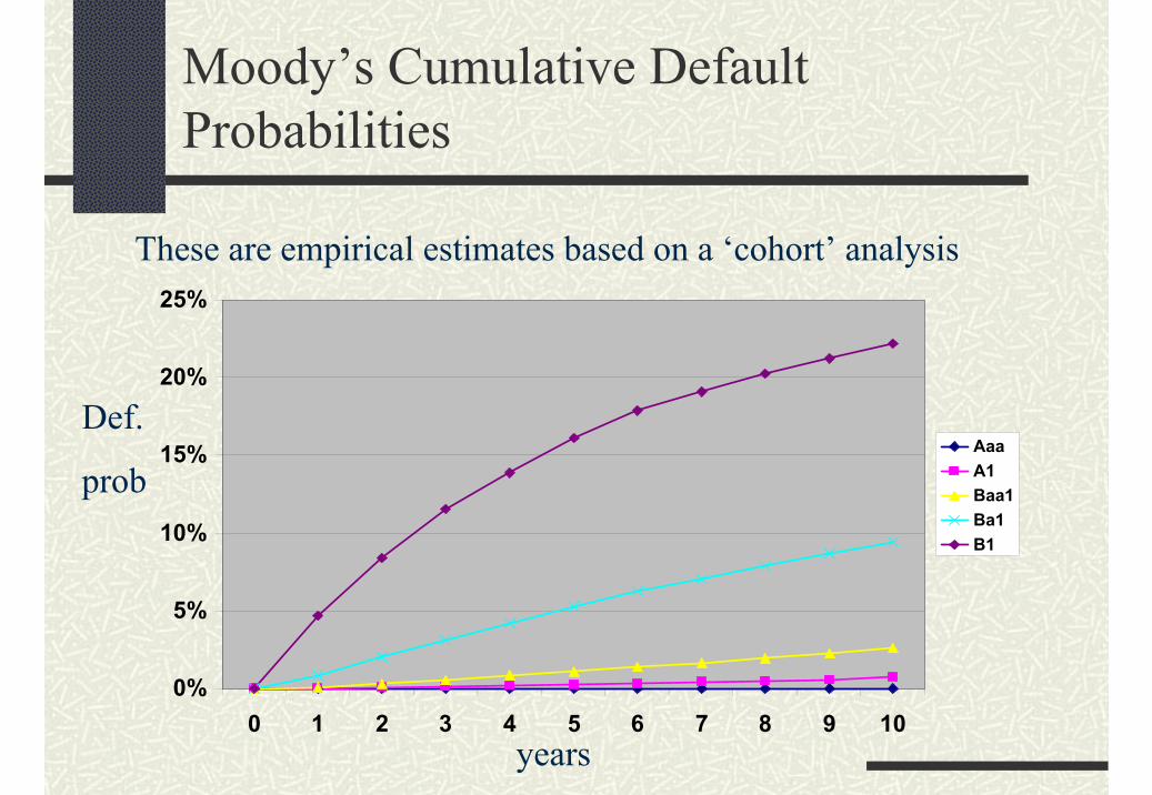
Moody’s Cumulative Default Probabilities
These are empirical estimates based on a ‘cohort’ analysis
0%
5%
10%
15%
20%
25%
0 1 2 3 4 5 6 7 8 9 10
AaaA1Baa1Ba1B1
years
Def.
prob
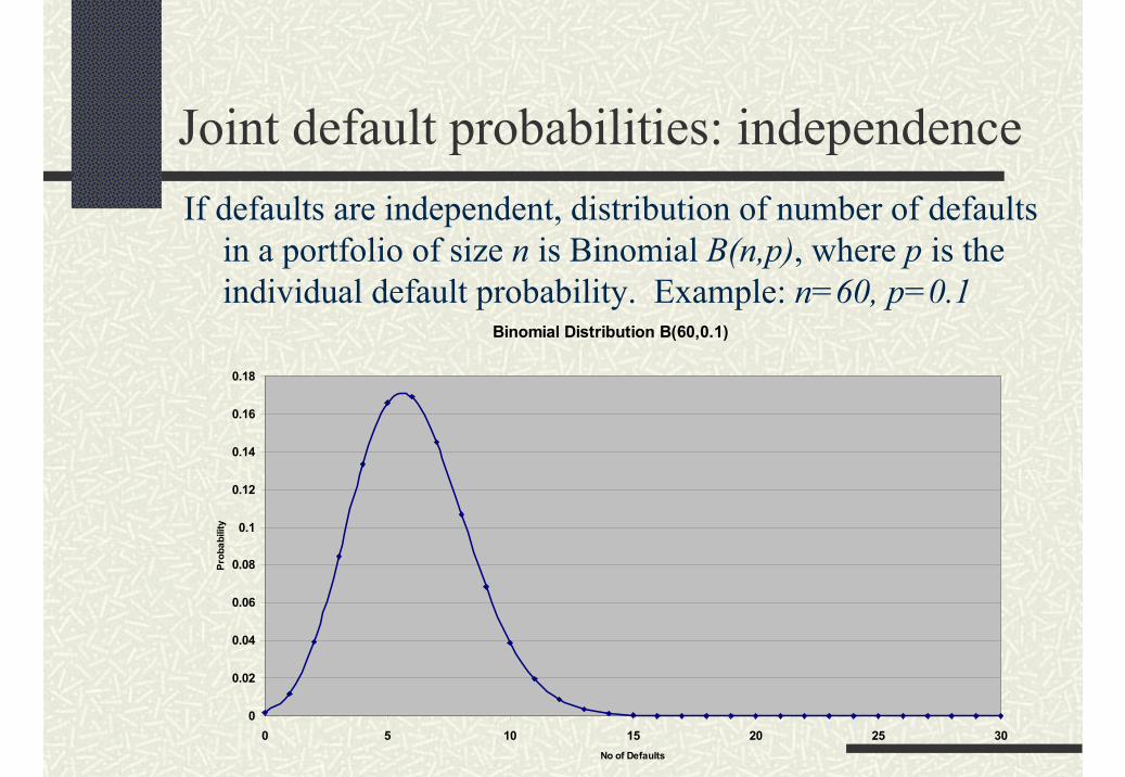
Joint default probabilities: independenceIf defaults are independent, distribution of number of defaults
in a portfolio of size n is Binomial B(n,p), where p is the individual default probability. Example: n=60, p=0.1
Binomial Distribution B(60,0.1)
0
0.02
0.04
0.06
0.08
0.1
0.12
0.14
0.16
0.18
0 5 10 15 20 25 30No of Defaults
Prob
abili
ty

Moody’s Binomial Expansion Technique
Start with a portfolio of M bonds, each (for simplicity) having the same notional value X. Each issuer is classified into one 32 industry classes. The portfolio is deemed equivalent to a portfolio of M’<M Independent bonds, each having notion value XM/M’. M’ is the diversity score, determined from the following table:
ind

Diversity score table
4.0102.65
3.792.34
3.582.03
3.271.52
3.061.01
Diversity score
No. of firms in same industry
Diversity score
No. of firms in same industry
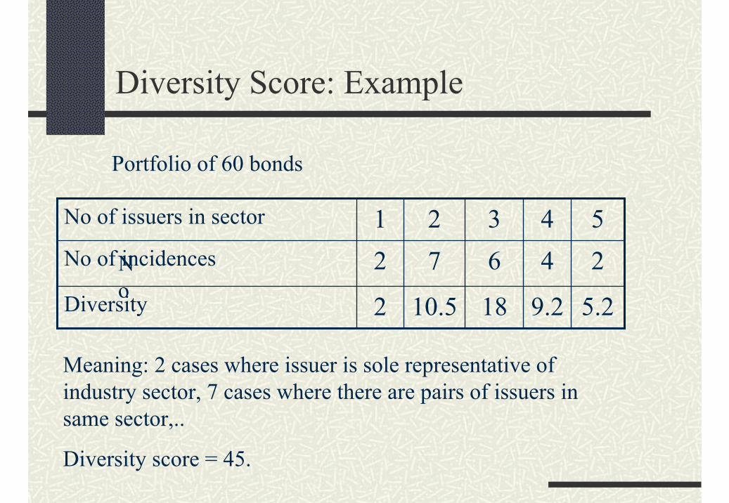
Diversity Score: Example
Portfolio of 60 bonds
No
5.29.21810.52Diversity
24672No of incidences
54321No of issuers in sector
Meaning: 2 cases where issuer is sole representative of industry sector, 7 cases where there are pairs of issuers in same sector,..
Diversity score = 45.
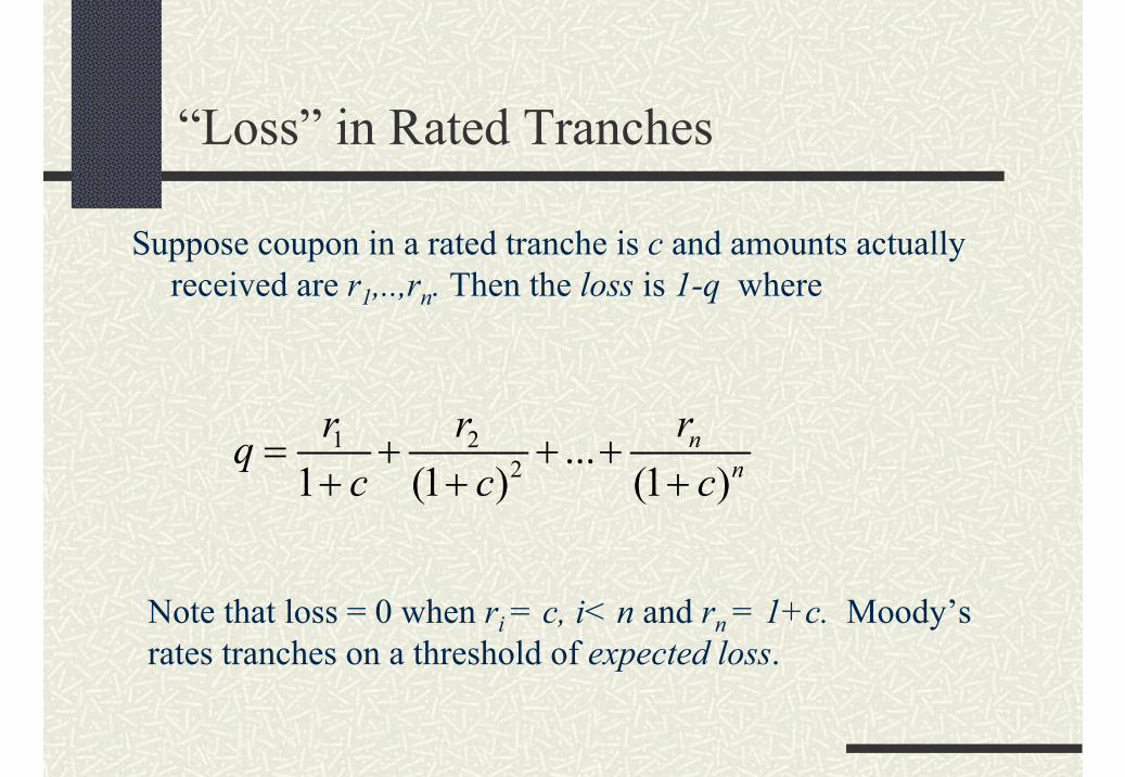
“Loss” in Rated Tranches
Suppose coupon in a rated tranche is c and amounts actually received are r1,..,rn. Then the loss is 1-q where
1 22 ...
1 (1 ) (1 )n
n
rr rqc c c
= + + ++ + +
Note that loss = 0 when ri = c, i< n and rn = 1+c. Moody’s rates tranches on a threshold of expected loss.
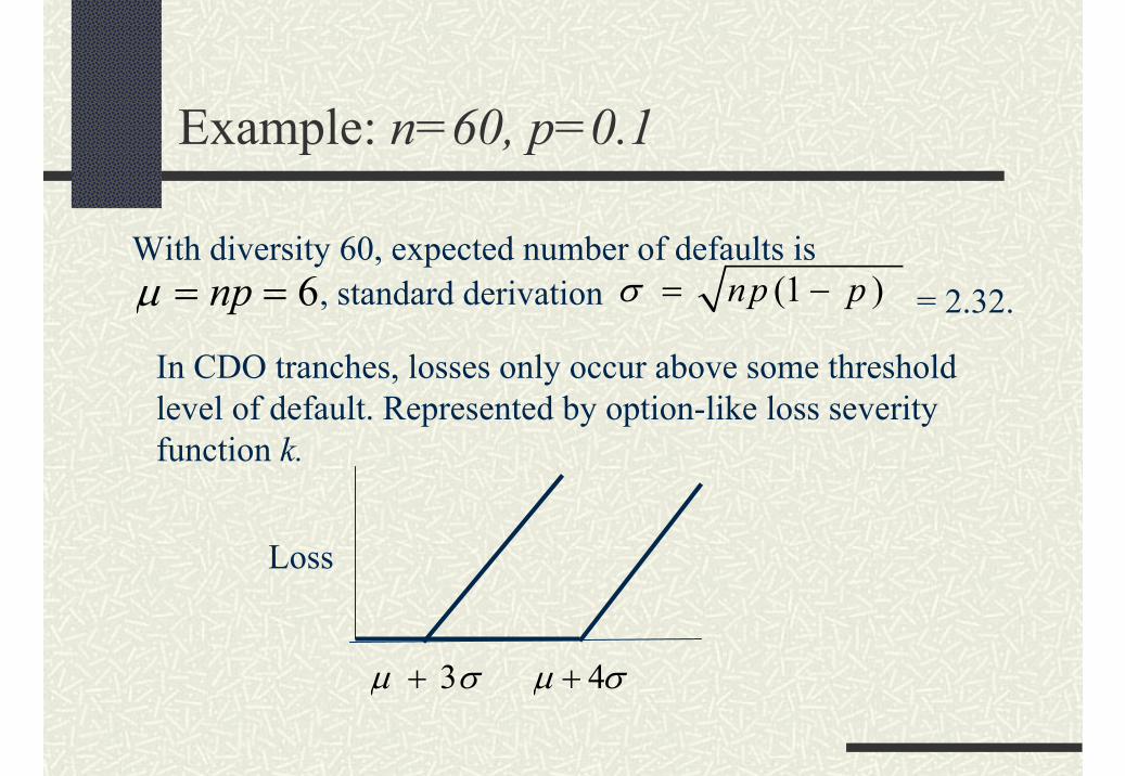
Example: n=60, p=0.1
With diversity 60, expected number of defaults is(1 ) np pσ = −, standard derivation 6npµ = = = 2.32.
In CDO tranches, losses only occur above some threshold level of default. Represented by option-like loss severity function k.
Loss
4µ σ+3µ σ+
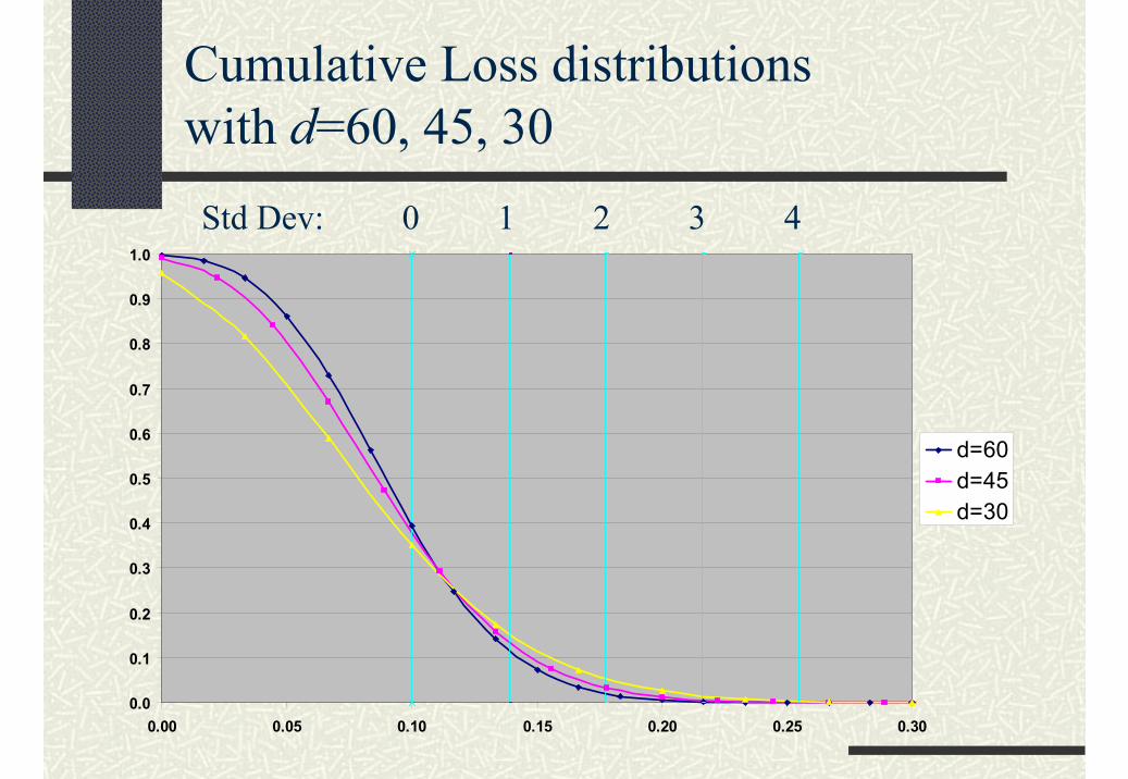
Cumulative Loss distributions with d=60, 45, 30Std Dev: 0 1 2 3 4
0.0
0.1
0.2
0.3
0.4
0.5
0.6
0.7
0.8
0.9
1.0
0.00 0.05 0.10 0.15 0.20 0.25 0.30
d=60d=45d=30
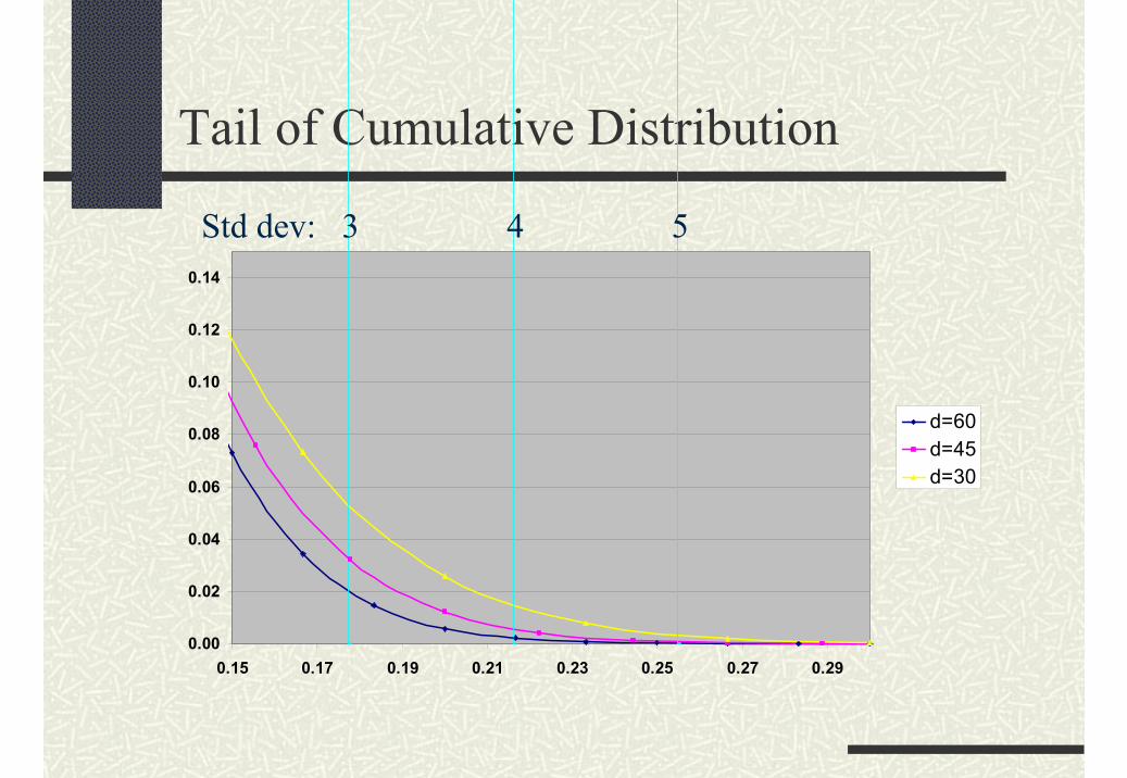
Tail of Cumulative Distribution
0.00
0.02
0.04
0.06
0.08
0.10
0.12
0.14
0.15 0.17 0.19 0.21 0.23 0.25 0.27 0.29
d=60d=45d=30
Std dev: 3 4 5
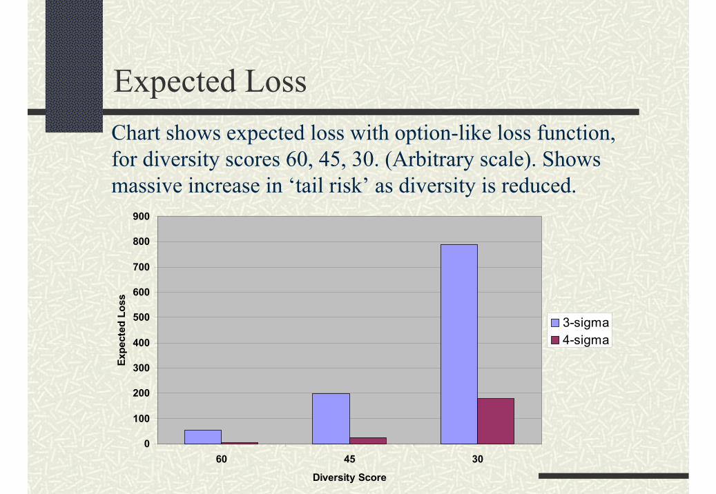
Expected LossChart shows expected loss with option-like loss function, for diversity scores 60, 45, 30. (Arbitrary scale). Shows massive increase in ‘tail risk’ as diversity is reduced.
0
100
200
300
400
500
600
700
800
900
60 45 30
Diversity Score
Expe
cted
Los
s
3-sigma4-sigma
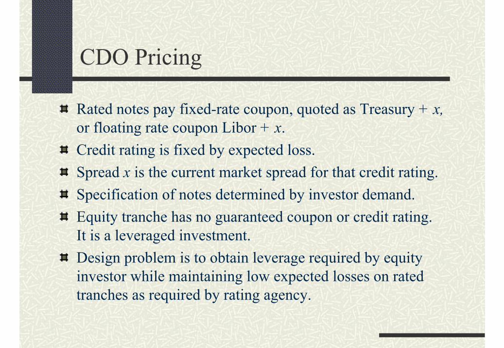
CDO Pricing
Rated notes pay fixed-rate coupon, quoted as Treasury + x, or floating rate coupon Libor + x.Credit rating is fixed by expected loss.Spread x is the current market spread for that credit rating.Specification of notes determined by investor demand.Equity tranche has no guaranteed coupon or credit rating. It is a leveraged investment.Design problem is to obtain leverage required by equity investor while maintaining low expected losses on rated tranches as required by rating agency.
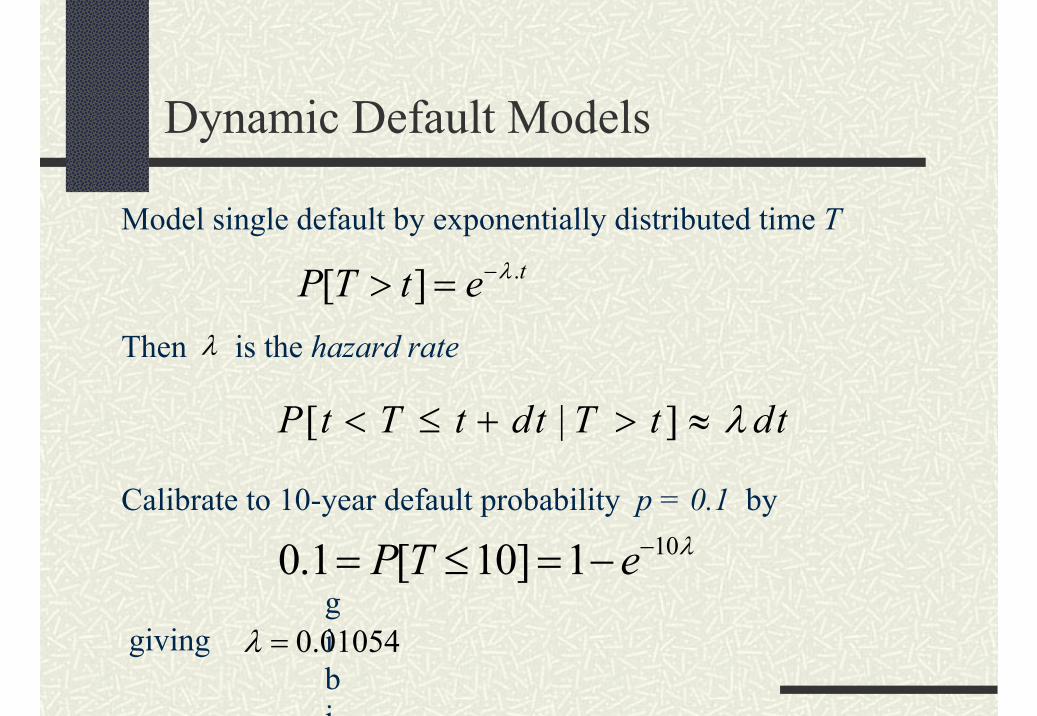
Dynamic Default Models
Model single default by exponentially distributed time T
Then is the hazard rate
Calibrate to 10-year default probability p = 0.1 by
.[ ] tP T t e λ−> =
[ | ]P t T t dt T t dtλ< ≤ + > ≈
100.1 [ 10] 1P T e λ−= ≤ = −gibi
giving 0.01054λ =
λ
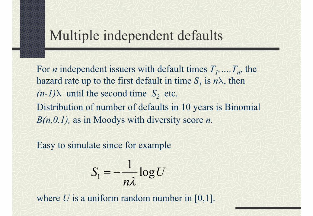
Multiple independent defaults
For n independent issuers with default times T1,…,Tn, thehazard rate up to the first default in time S1 is nλ, then(n-1)λ until the second time S2 etc. Distribution of number of defaults in 10 years is Binomial B(n,0.1), as in Moodys with diversity score n.
Easy to simulate since for example
where U is a uniform random number in [0,1].
11 logS U
nλ= −
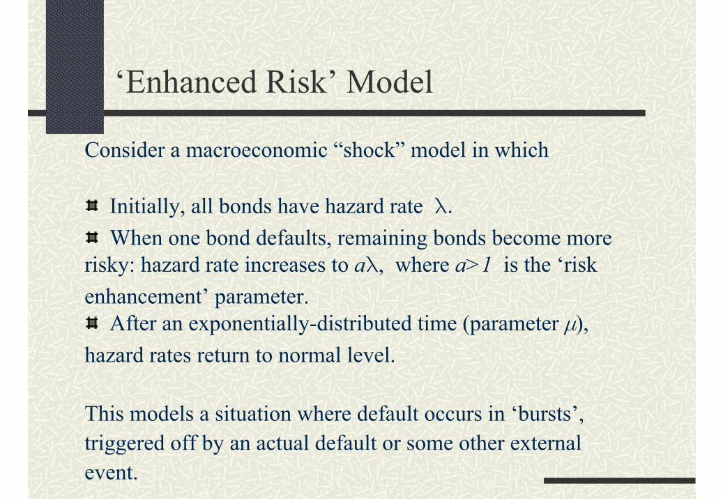
‘Enhanced Risk’ Model
Consider a macroeconomic “shock” model in which
Initially, all bonds have hazard rate λ. When one bond defaults, remaining bonds become more
risky: hazard rate increases to aλ, where a>1 is the ‘risk enhancement’ parameter.
After an exponentially-distributed time (parameter µ), hazard rates return to normal level.
This models a situation where default occurs in ‘bursts’, triggered off by an actual default or some other external event.

Markov Process Specification
Enhanced risk model is Markov process on state spaceE = {(i,j): i=0, 1; j=0,1,…,n}. Index i=0 represents ‘normal risk’ and i=1 represents ‘enhanced risk’. Transition rates between states are shown on next slide.
Simulation is simple because sojourn times in each stateare exponential – same relation with uniform randomnumbers as before.
Computation of distributions and expectations only involves solving ordinary differential equations.
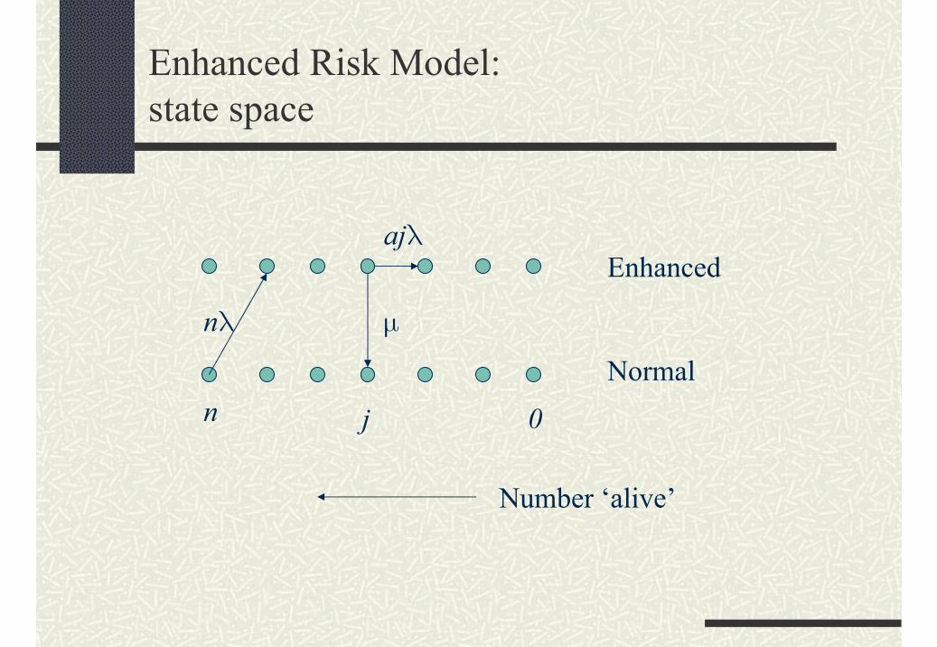
Enhanced Risk Model:state space
n 0j
Enhanced
Normal
nλ µ
ajλ
Number ‘alive’
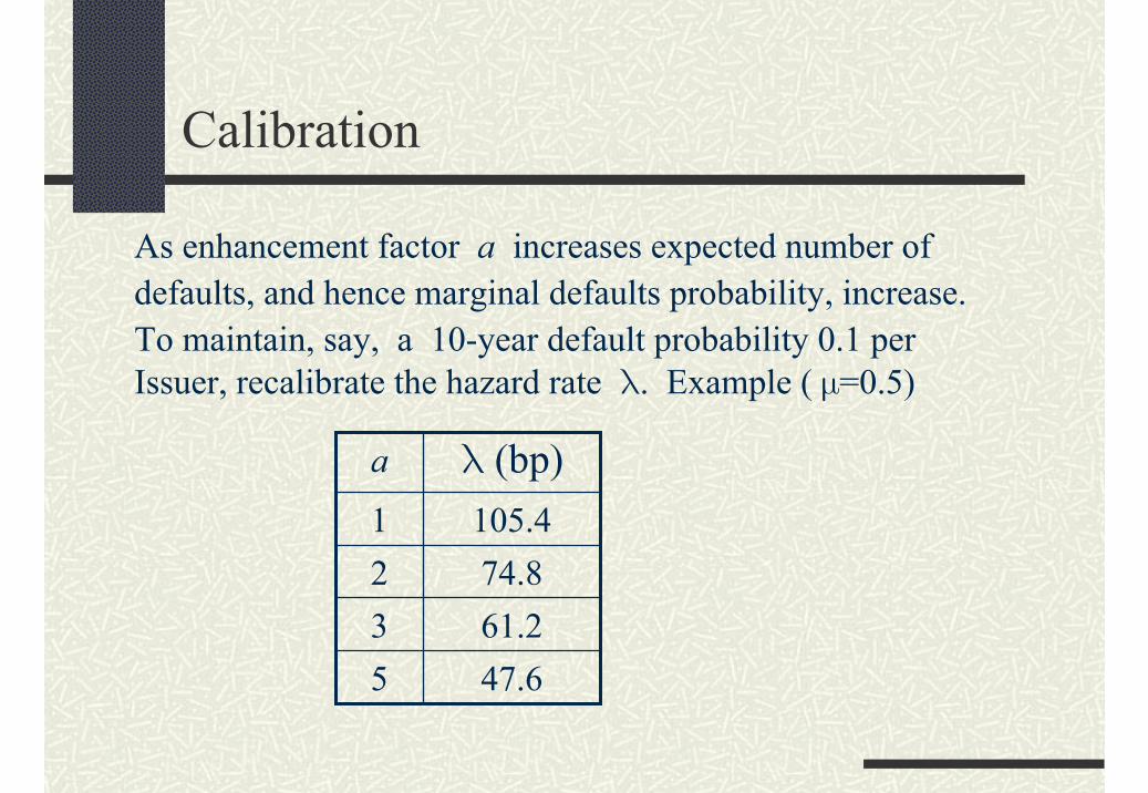
Calibration
As enhancement factor a increases expected number of defaults, and hence marginal defaults probability, increase.To maintain, say, a 10-year default probability 0.1 per Issuer, recalibrate the hazard rate λ. Example ( µ=0.5)
47.6561.2374.82105.41
λ (bp)a
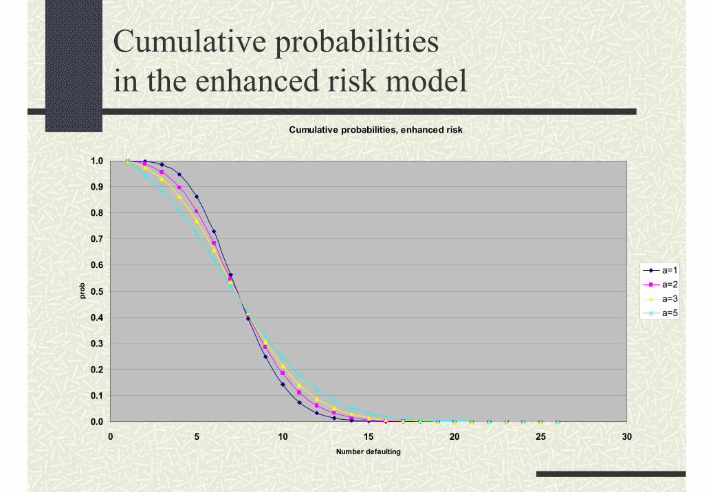
Cumulative probabilitiesin the enhanced risk model
Cumulative probabilities, enhanced risk
0.0
0.1
0.2
0.3
0.4
0.5
0.6
0.7
0.8
0.9
1.0
0 5 10 15 20 25 30Number defaulting
prob
a=1a=2a=3a=5
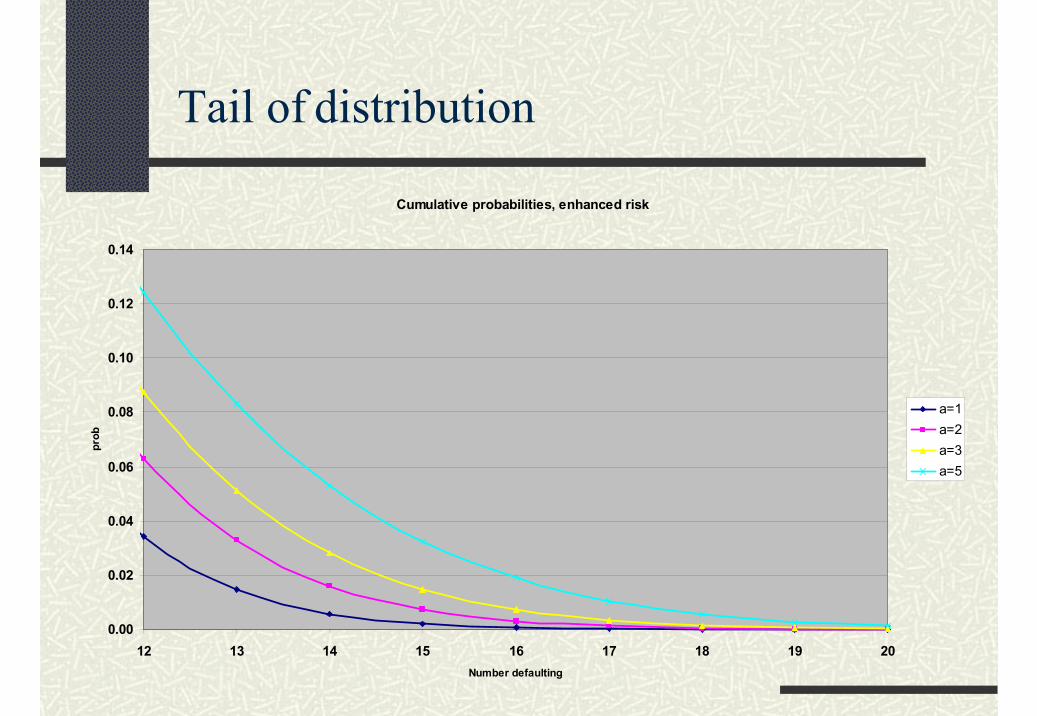
Cumulative probabilities, enhanced risk
0.00
0.02
0.04
0.06
0.08
0.10
0.12
0.14
12 13 14 15 16 17 18 19 20Number defaulting
prob
a=1a=2a=3a=5
Tail of distribution
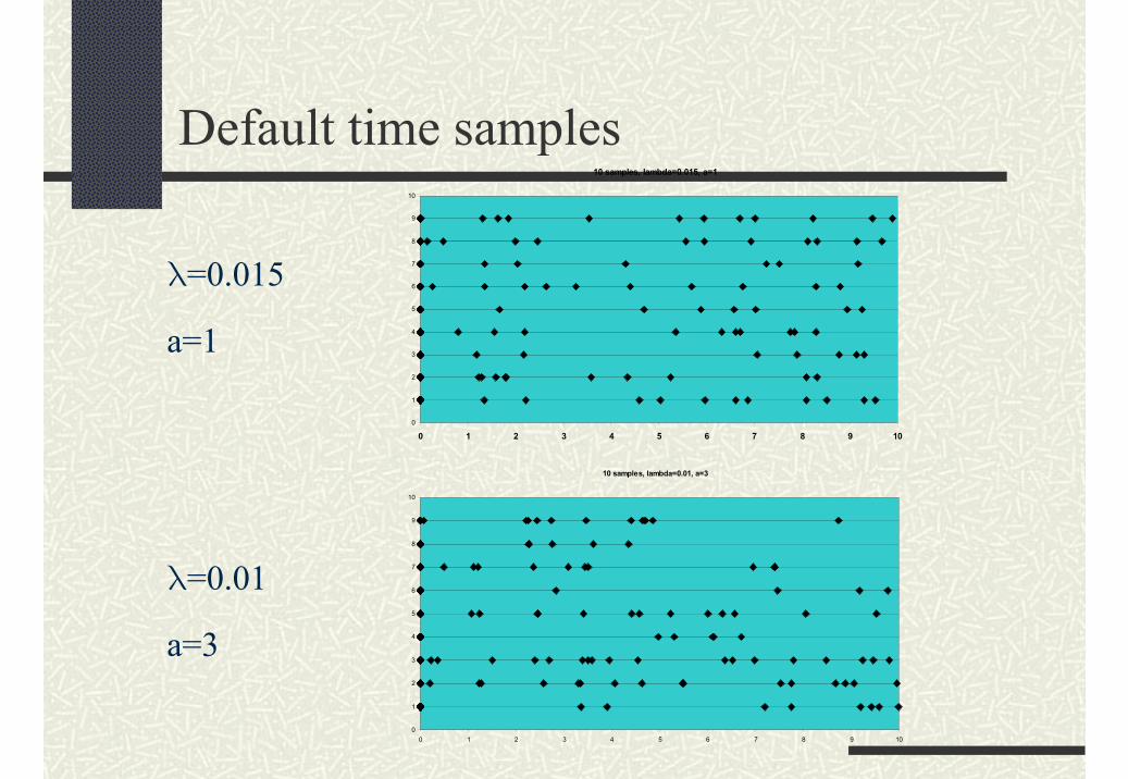
Default time samples10 samples, lambda=0.015, a=1
0
1
2
3
4
5
6
7
8
9
10
0 1 2 3 4 5 6 7 8 9 10
λ=0.015
a=1
λ=0.01
a=3
10 samples, lambda=0.01, a=3
0
1
2
3
4
5
6
7
8
9
10
0 1 2 3 4 5 6 7 8 9 10
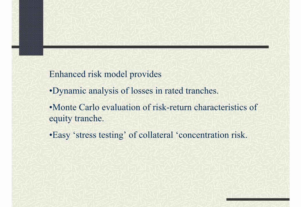
Enhanced risk model provides
•Dynamic analysis of losses in rated tranches.
•Monte Carlo evaluation of risk-return characteristics of equity tranche.
•Easy ‘stress testing’ of collateral ‘concentration risk.
Summary
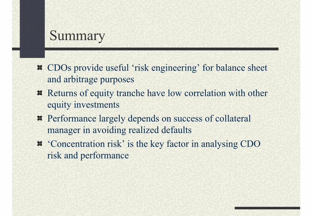
CDOs provide useful ‘risk engineering’ for balance sheet and arbitrage purposesReturns of equity tranche have low correlation with other equity investmentsPerformance largely depends on success of collateral manager in avoiding realized defaults‘Concentration risk’ is the key factor in analysing CDO risk and performance
References
CDO Handbook, J.P. Morgan Global Structured Finance Research, May 2001, www.morganmarkets.comMark Davis and Violet Lo, Modelling default correlation in bond portfolios, in Mastering Risk Volume 2: Applications, ed. Carol Alexander, Financial Times Prentice Hall 2001, pp 141-151, www.ic.ac.uk/~mdavis