Collateral Reuse and Business Cycle

Hyejin Park∗

Last updated: November 1, 2016

Abstract

I study the dynamics of an economy relying on collateral reuse subject toaggregate uncertainty that collateral chains might fail. In the model, collat-eral reuse has two opposing effects: it helps financing additional investment bymaking scarce collateral support multiple loans at once; but it might lead tomismatch between collateral and an investment opportunity in the event thatintermediaries in the middle of collateral chains fail. In such circumstances,I discuss how individual reuse decisions, collateral allocations, and aggregateoutput vary: (i) across different temporary unexpected shocks; (ii) across dif-ferent persistent shocks. The analysis shows that: the size of crisis can begreater and the speed of recovery can be faster as a shock is worse; continuedbad shocks might lead to a greater increase in output once the recession ends,and conversely, continued good shocks might lead to a greater decrease in out-put once the boom ends. These results shed light on the discussion on how toregulate rehypothecation after the financial crisis.

1 Introduction

At the center of the financial crisis, there were failures of large dealer banks thatintermediated in the market for over-the-counter (OTC) derivatives and repurchaseaggrements (repos). Examples are the bankruptcy of Lehman Brothers and BearSterns. The failures of these banks were prompted and accelerated by runs of theirclients. For example, as Lehman Brothers headed towards bankruptcy, hedge funds

∗Department of Economics, University of Illinois at Urbana-Champaign. E-mail:park354@illinois.edu. I thank my advisor Charles M. Kahn for his advice and guidance. I alsothank Dan Bernhardt, Jorge Lemus, and Guillermo Marshall for helpful comments and sugges-tions.

1

who were concerned about the solvency of their dealer banks – these also includedmajor dealer banks such as Morgan Stanley and Goldman Sachs – raced to withdrawtheir assets from these banks, shifting them into other commercial banks deemedsafer, thereby weakening the banks’ capital position.

The concerns of these hedge funds over the solvency of the dealer banks wererooted in the deepest part of the business of these banks: rehypothecation, a practicein which banks reuse or repledge parts of their clients’ collateral to support their ownloans. Before the crisis, this collateral reuse was a prevalently used technique of dealerbanks to raise extra liquidity. After the failure of Lehman Brothers, however, manyclients of these dealer banks, especially, hedge funds, were concerned about losingaccess to their collateral,1 and did not allow the banks to reuse their collateral.2 Sincethen, collateral reuse has received extensive attention as an important factor thatcontributed the severity of the crisis. In particular, the need to study the economiceffects of this practice has been emphasized.3

This paper studies the role of collateral reuse in the business cycle. In this paper,I ask the following questions: When is collateral reuse more likely to occur? Howdoes a shock that increases the risk of failure by dealer banks (that is, the probabilitythat the banks default having repledged their clients’ collateral to the other parties)initiate fluctuations in aggregate output? How does the shock affect the individuals’preferences over collateral reuse? When do the borrowers agree with reusing theircollateral? What would be the effects of these agents’ choices of collateral reuse onoutput dynamics and the speed of recovery after adverse shock?

To answer these questions, I build a dynamic model in which collateral reuseworks as a channel that transmits a temporary shock to the macro economy. The

1This is because in most case, if a bank defaults having repledged their clients’ collateral, thatcollateral will be seized by third parties to whom the bank repledged it. For example, hedge fundsthat used Lehman Brothers such as GLG Partners, Amber Capital and Ramius were not able toaccess the assets of $40 billion held by the European branch of Lehman Brothers (Mackintosh,2008), and Olivant, the investment company that used Lehman Brothers could not participate invoting at UBS’s shareholder meeting since its 700 miliion pound shares in UBS were tied up atLehman (Farrell, 2008).

2Singh (2010) reports that the value of rehypothecatable assets that Morgan Stanley receivedfrom its clients decreased from $953 million in May 2008 (the peak) to $294 million in Nov 2008.Over the same period, the decrease in the amount of rehypothecatable collateral by Goldman Sachsand Merrill Lynch are about 66% and 38%, respectively.

3However, there are still differences in the regulation of collateral reuse across countries. Forexample, problems stemming from rehypothecation failure are more severe in Europe than in the US,since in Europe, especially in the UK, there was no limit on the amount that can be rehypothecatedby broker-dealers, but in the US, SEC rule 15c3-3 restricts the amount of client assets that can berehypothecated to no more than 140% of the value of the client’s liability.

2

aggregate output generally depends on the relative size of two trade-off effects ofcollateral reuse: (1) a positive effect that additional investment activities can befinanced by reusing collateral; and (2) a negative effect that collateral might end upwith the wrong hands (who does not have technology to use that collateral efficiently)in the event that the intermediary in the middle of the collateral chain defaults.

It is noteworthy that the intermediary’s risk of failure tends to be countercyclical– the risk of default of the dealer banks is low in booms and high in recessions.Therefore, in booms, the positive effect to increase liquidity supply tends to exceedthe negative effect to cause collateral misallocation, increasing overall level of output;and the opposite happens recessions.

For the same reason, if there is an unexpected shock that increases the risk offailure of the intermediary, the cost of misallocating collateral tends to outweighthe benefits of financing additional projects, causing aggregate output to decrease.More importantly, the shock can have another indirect effect on the output dynamicsby altering individual choice over collateral reuse: the initial pledgor can forbid itscounterparty from reusing its collateral if the risk of losing collateral seems too high.

Therefore, there are two possible scenarios after the shock: (i) If the shock isrelatively small, the borrower will continue allowing collateral reuse. As a result,the size of the crisis at the time of the shock will be relatively small, but it tends befollowed by a long economic downturn. The downturn reflects that allowing collateralreuse at the time of the shock increases misallocation of collateral in the future, sothat the aggregate output remains below its previous steady state until the collateralis re-allocated back to its most efficient uses; (ii) If the shock is relatively large, theborrower will be reluctant to allow collateral reuse. As a result, the size of the crisiswill be relatively large since additional productive investments cannot be financed.However, the speed of recovery will be faster, because precluding collateral reuseat the time of the shock has a positive effect of decreasing collateral misallocation,thereby increasing the speed of recovery – aggregate output can be even greaterthan its previous steady state, provided that there exists initially a (small) positiveprobability of misallocating collateral before the shock.

Next, I contrast outcomes across different persistent shocks, one history of shocksis uniformly better than another. I show that as a good state continues, borrowersallow collateral reuse more frequently, and misallocation of collateral increases, sow-ing the seeds for a greater decrease in output when the boom ends. Conversely, asbad state continues, collateral reuse occurs less frequently, misallocation of collateraldecreases, setting the stage for greater increase in output when the recession ends.

The paper starts with a simple discrete-time, infinite horizon model with a contin-uum of ex-ante identical agents. At the beginning of each period each agent receives

3

either an investment opportunity that requires cash as input to produce more cashat the end of the period, or cash that can be consumed or used as inputs for theinvestment. Thus, no one can have both the investment opportunity and cash atthe same time – there is a mismatch between production opportunity and inputs.In addition, I assume that the probability of investment oppportunities is persistent:if an agent receives an investment opportunity today, he is more likely to have aninvestment opportunity tomorrow than an agent who does not receive one today –this persistency of the roles as borrowers and lenders is typical in the repo markets.

In this setting, a project can be undertaken only if cash holders provide fundingto the project’s owner. However, the future return of the project may not be enoughto guarantee repayment of the loan, and borrowing only backed by the future returnof the project may not be feasible. For example, such limited pledgeability of theborrower could reflect moral hazard: he might want to divert the funding that hereceived for his private benefit. In such circumstance, requiring the borrower to postother valuable assets (which might be separate from the project) as collateral canincrease credit; it gives the borrower incentive to repay the loan to avoid forfeitingit.4

I assume that there is a long-term indivisible asset that delivers a constant divi-dend for an infinite period that can serve as collateral – one can think of this asset asa perpetuity. Thus, when agents cannot store cash (or they have limited capacity tostore cash), only this asset can be used as collateral in this simple setting. I assumethat the collateral asset is scarce in the sense that the total asset endowment is lessthan the cash endowment, following the emprical results shown by Krishnamurthyand Vissing-Jorgensen (2013) and Greenwood et al. (2010).

Based on these assumptions, at any given point of time, there are four types ofagents: those who have both an investment opportunity and collateral (denoted bytype AZ), those who have only an investment opportunity (type A0), those who havecash and collateral (type CZ), and those who have only cash (type C0). I assumethat each agent can hold one collateral asset at most, and only the cash holders whodo not hold collateral (that is, type C0) can participate in collateralized lending.One the other side, only type AZ agents will become borrowers.5 Then, I assumethat type AZ agents are randomly matched with type C0 agents and they optimallychoose the size of loan and repayment.

4In general, collateral plays two important roles as hostage and as insurance, as explained byMills and Reed (2012). For ease of exposition, I focus on the role of collateral as hostage in thissimple setting.

5Agents type A0 ‘cannot’ borrow since they do not have collateral asset, and agents type CZ‘do not want’ to borrow since they do not have projects.

4

The contracting problem between type AZ and type C0 agents within a singleperiod is like that in the two-agent model in Kahn and Park (2016), in which theoptimal collateralized debt contract maximizes the borrower’s utility subject to theincentive constraint of the borrower and the rationality constraint of the lender.Then, based on the analysis in a single period, I characterize the steady state ofthis economy, and study the comparative statics of the steady state to show how theequilibrium mass of types depends on the persistency of investment opportunities –with more focus on the mass of type AZ, since this is a critical variable determiningthe number of projects that can be financed.

Next, I extend the model to three agents to incorporate the possibility of reusingcollateral. Each period, type AZ agents enter into a collateralized debt contract withthe intermediary, who subsequently enters a collateralized debt contract with type C0agents, by reusing the collateral received from type AZ agents – a typical example ofthe intemediary is broker-dealer bank such as Lehman Brothers, Bear Sterns, and soon. The optimal contract within a single period then can be obtained by backwardinduction, and the steady state can be found by using the same approach in thebaseline model.

The model shows that the possibility of collateral reuse by the intemediary de-livers the two main effects mentioned earlier: it allows for additional productiveinvestment by the intermediary, but it may lead to mismatch between collateral andproduction in the event that the collateral chain fails. I assume that the probabilityof the failure to return collateral is exogenously given, and I analyze the fluctuationsin output when there is a negative temporary shock that increases this probabilityof losing collateral. I find that there are the two possible paths after the shock: onein which the borrowers allow collateral reuse at the time of the shock and another inwhich they preclude it. I find that the size of crisis tends to be bigger in the formercase, but the recovery speed tends to be faster in the latter case.

I intend to extend the model to introduce an asset market each period, so thattype AZ agents who lose the collateral can purchase the collateral from type CZagents (or type C0 agents if they have collateral after the failure of the intermediary).I expect that the main results will be untouched, as long as the asset market is notfrictionless, and so the collateral misallocated due to the negative shock will not bepromptly returned to agents with investment opportunities.

The structure of the paper is as follows. Section 2 builds the simple dynamicmodel of collateralized lending between two agents. Section 3 adds in the intermedi-ary to incorporate the possibility of collateral reuse. Section 4 introduces a shock andstudy the output dynamics. Section 5 provides numerical examples of the dynamics.The final section concludes.

5

2 Simple Two Agent Model – without Collateral

Reuse

In this section I describe the baseline model with two agents in which a borrowerhas to post his valuable asset as collateral to the lender in order to receive fundingfor his productive investment. I then extend the model to three agents in which theintermediary can repledge his borrowers’ collateral to the third party.

2.1 Setting

Time is descrete with an infinite horizon and each period is indexed by t. Thereare two types of agents, borrowers and lenders. Both agent types are risk neutral witha common discount factor β ∈ (0, 1). An agent can become either an entrepreneuror a cash investor in each period, depending on his endowment in that period: hemight have an investment opportunity but has no cash, or he might be endowed withcash but has no investment opportunity.

The investment opportunity requires cash as an input to produce more cash atthe end of the period, yielding R > 1 units of cash per unit of input. This impliesthat it is potentially useful to transfer cash from a cash holder to an entrepreneur’sproject.

However, the entrepreneur has the option to divert the funds that he borrowedfor his private benefit (‘absconding’ as in Calomiris and Kahn (1991)). The privatebenefit from diverting is b per unit of funds diverted, which is assumed to be nottransferable. If this benefit from diverting is sufficiently large, without any externalmeans of forcing repayment of the loan, cash holders would not be willing to providecash to entrepreneurs.

One simple way to restore credit in such circumstances is to make the borrowerpost other valuable assets (which might be separate from this project) as collateral.I assume that the borrower has one unit of indivisible asset which yields one unitof cash at the end of each period – one can think of this asset as a perpetuity withconstant dividends. With the borrower’s asset in hand, the lender is now assuredthat the borrower will repay the loan, since the borrower has now an incentive torepay to avoid forfeiting the collateral (and so, collateral acts like a hostage)6

In this setting, there are two types of goods: the collateral asset and cash. Iassume that cash is not storable, depreciating completely if not consumed imme-diately. In contrast, the collateral asset is storable, producing constant dividends

6In general, collateral also provides a lender with recourse to collect revenue by liquidating itin the event that the borrower defaults, that is, collateral can play an insurance role.

6

forever (and this durability renders the asset acceptable as collateral). I assume thateach agent can store only one unit of the collateral asset, that is, each agent has alimited capacity of storage. In addition, I assume that the asset is endowed to agentsonly in the initial period, t = 0, and so the total amount of the asset is fixed in allperiods. Lastly, I assume that the asset market is not available, and it is not possiblefor the agents to buy or sell the asset (in future research, I will extend the model toallow for an asset market in which they can trade the asset).

Investment opportunities arrive randomly. I assume that the probability of re-ceiving an investment opportunity in the next period depends on the state of anagent in the current period; if an agent has an investment opportunity today, thenhe will have an investment opportunity again tomorrow with probability p, and withsymmetry, if that person does not have an investment opportunity today, he will notreceive an investment opportunity with probability p. When p > 1

2, the investment

opportunity is persistent.As a result, there are two state variables: (1) an agent has an investment oppor-

tunity or not (have cash instead of the investment opportunity); and (2) an agenthas the collateral asset or not. This implies that at any given point of time thereare four types of agents: those who have both the investment opportunity and thecollateral asset, denoted by type “AZ,” those who have the investment opportunitybut do not have the collateral asset, type “A0,” those who do not have the invest-ment opportunity but have the collateral asset, type “CZ,” and lastly, those whohave neither the investment opportunity nor the collateral asset, type “C0.”

Note that only agents who have both the investment opportunity and the asset(type AZ) can undertake the investment, because an agent is able to borrow fundingfor his project only if he can post collateral. I assume that only type C0 agents whodo not hold the asset can participate in the collateralized lending market, while typeCZ agents remain outside of the market and consume the cash endowment at thattime – one can interpret that they have already hold the asset and have no capacitiyto hold the borrower’s collateral.

Then, type AZ and C0 agents are randomly matched each other in each periodand optimally choose the condition of the collateralized debt contracts. To facilitateanalysis, I assume that in any period t, the mass of type AZ agents (borrowers),denoted by MAZt, is less than the mass of type C0 agents (lenders), denoted byMC0t. This means that and type AZ agents can always borrow cash.

Assumption 1. MAZt ≤MC0t for all t.

Combining all the assumptions so far, the evolution of the distribution of typescan be represented as follows.

7

MAZt+1

MA0t+1

MCZt+1

MC0t+1

=

p 0 1− p 00 p 0 1− p

1− p 0 p 00 1− p 0 p

MAZt

MA0t

MCZt

MC0t

(1)

where p ∈ (0.5, 1].

2.2 Optimal Contract within a Single Period

I now solve for the optimal short-term collateralized debt contract between typeAZ and type C0 agents within a single period. This single period model builds onthe framework in Kahn and Park (2016) in which the optimal collateralized debtcontract solves the borrower’s incentive problem. Following their approach, I focuson the case in which the optimal contract satisfies the incentive constraint of theborrower, that is, the optimal contract induces the borrower not to divert the fundshe receives (the conditions for this to be the optimal choice are provided in Kahnand Park (2016)).

The timing is as follows:

• At the beginning of each period, an investment opportunty randomly arrives toeach agent. If an agent has the investment opportunity (becomes type A), heborrows funds IA for his investment from a cash investor who has a sufficientlylarge amount of cash by posting collateral (provided that he has the collateralasset at that time) and promises to pay an amount XA in exchange for receivingthe collateral at the end of the period.

• At the end of the period, the investment yields the outcome RIA (provided thatthe borrower does not divert the funds he receives) and the borrower receivesthe collateral back in return for paying the lender the prearranged amount XA.

The value of holding the collateral asset might differ between different types. Idenote the value of the asset for agent type s by Vs where s ∈ {AZ,A0, CZ,C0}.For simplicity, for the single-period analysis, I assume that these value functions aregiven (I will show that these values are endogenously determined in the next section).Finally, I assume that the borrower holds all bargaining power (that is, the lendingmarket is competitive).

Then, taking the value of holding collateral for the borrower VAZ and the lenderVC0 as given, the optimal contract (IA, XA) solves,

maxIA,XA

RIA −XA + {1 + β[pVAZ + (1− p)VCZ ]} (2)

8

subject to

RIA −XA + {1 + β[pVAZ + (1− p)VCZ ]} ≥ bIA (ICB)

XA − IA ≥ 0 (IRL)

The objective function is the borrower’s utility. The term RIA is the return from theinvestment, the term XA is the repayment in exchange for receiving the collateral, 1is the dividend from the collateral in the current period, and β[pVAZ + (1 − p)VCZ ]is the expected value of the collateral to the borrower: the value of the collateralbecomes VAZ if he receive an investment opportunity andVCZ if he does not receivean investment opportunity, and p is the probability of receiving an investment op-portunity again in the next period.

The first constraint (ICB) is the incentive constraint of the borrower: the lefthand side is the profit if he fulfills the obligation and the right hand side is theprivate benefit if he diverts the funds. The second constraint (IRL) is the partici-pation constraint for the lender that his profit from lending cannot be less than thereservation value which is set to be zero.

Under the assumption that R > 1, the linearity of the problem ensures thatboth contraints (ICB) and (IRL) bind at the optimum. Solving these two equationssimultaneously yields the optimal contract in a single period.

Lemma 1. Suppose the value function of the borrower VAZ and the lender VCA aregiven exogenously. The optimal contract within a single period is given by a pair(IA, XA) such that

IA = XA =1 + β[pVAZ + (1− p)VCZ ]

b+ 1−R. (3)

To implement this contract, the collateral has to be more valuable to the borrowerthan it is to the lender, so that the borrower wants to retrieve it from the lender expost, that is,

1 + β[pVAZ + (1− p)VCZ ] > 1 + β[pVCZ + (1− p)VAZ ] (4)

The left hand side is the value of the collateral to the borrower and the right handside is the value of the collateral to the lender. Rearranging the terms, this can berewritten as follows.

(2p− 1)(VAZ − VCZ) > 0 (5)

Thus, if VAZ > VCZ (which will turn out to hold in equilibrium in the next section),

9

this condition implies that the borrower wants to retrieve the collateral only if 2p−1 > 0, that is, investment opportunities are persistent. Thus, I make the followingassumption.

Assumption 2. p ∈(

12, 1].

2.3 Stationary Equilibrium

Based on the single-period analysis I now solve for a stationary equilibrium andprovide comparative statics at the steady state. To begin, I define an equilibrium ofthis dynamic economy as follows.

Definition 1. A stationary equilibrium is a profile (IA, XA,MAZ ,MA0,MCZ ,MC0)that satisfies:

• (IA, XA) is the optimal contract within a single period in Lemma 1

• (MAZ ,MA0,MCZ ,MC0) is a stationary distribution for (MAZt ,MA0t ,MCZt ,MC0t)in Equation (1) that remains constant over time.

2.3.1 Stationary Distribution of Agent Types

First, I solve for the stationary distribution of agent types, (MAZ ,MA0,MCZ ,MC0),that satisfies Assumption 1 and Equation (1). For illustration, I assume that the ini-tial distribution is given as follows.

Assumption 3. The initial distribution of agent types (MAZ0 ,MA00 ,MCZ0 ,MC00)satisfies

– MA00 +MC00 ≥MAZ0 +MCZ0 (scarcity of collateral)

– MC00 +MCZ0 ≥MAZ0 +MA00 (scarcity of investment opportunities)

– MC00 ≥MAZ0

First, MA00 + MC00 ≥ MAZ0 + MCZ0 states that the mass of cash holders, typeA0 and C0, exceeds the mass of collateral holders, type AZ and CZ, implying thatcollateral is scarce. Second, MC00 + MCZ0 ≥ MAZ0 + MA00 states that the massof agents without investment opportunities, type C, exceeds the mass of agentswith investment opportunities, type A, implying that investment opportunities arescarce. Lastly, MC00 ≥ MAZ0 states that the number of lenders exceeds the numberof borrowers.

10

Under Assumption 1 and 3 and using Equation (1), I can show that the distri-bution of agent types evolves over time as follows.7

Lemma 2. Under Assumption 3, the mass of each agent type in period t is givenby,

MAZt =1

2[1 + (2p− 1)t]Z (6)

MA0t = 1−MC0t = 1− 1

2[1 + (2p− 1)t] (7)

MCZt = Z −MAZt = Z − 1

2[1 + (2p− 1)t]Z (8)

MC0t =1

2[1 + (2p− 1)t] (9)

and Assumption1 holds,

MAZt =1

2[1 + (2p− 1)t]Z <

1

2[1 + (2p− 1)t] = MC0t ∀t (10)

Then, it immediately follows that the limiting distribution for (MAZt ,MA0t ,MCZt ,MC0t)in Lemma 2 is the stationary distribution of agent types.

Corollary 1. Suppose Assumption 3 holds. In the unique stationary distribution ofagent types

MAZ = MCZ =1

2Z, MA0 = MC0 =

1

2. (11)

2.3.2 Value Functions

Next, I solve for the value functions of each type. First, the value function oftype C agent (the lender) is given by

VCZ = 1 + β[pVCZ + (1− p)VAZ ] (12)

Here, 1 is the dividend from the asset and the remaining terms are the expected valueof the collateral for a cash holder: with probability p, he has only cash again and thevalue of the asset becomes VCZ , and with probability 1 − p, he has an investmentopportunity and the value of the asset becomes VAZ .

7Recall that to apply Equation (1), the distribution must satisfy Assumption 1. In the proof, Iverify that the solution indeed satisfies Assumption 1, so that Equation (1) holds.

11

The value function of type A agent (the borrower) is given by,

VAZ = maxIA,XA

RIA −XA + {1 + β[pVAZ + (1− p)VCZ ]} (13)

where IA and XA are given in Lemma 1. As mentioned earlier, RIA − XA is thenet gain from the investment after paying the loan, and 1 is the dividend from thecollateral and the remaing terms reflect the expected value of the collateral to theborrower.

Then, solving the two equations (12) and (13) simultaneously reveals that thevalue functions take the following forms.

Lemma 3. The value function of type A agent (the borrower) and type C agent (thelender) are given by,

VAZ =γ[1− β(2p− 1)]

1− β{p+ γ[p− β(2p− 1)]}(14)

VCZ =1− βγ(2p− 1)

1− β{p+ γ[p− β(2p− 1)]}(15)

where γ ≡ b1+b−R > 1.

From this result, it follows that the value function of the borrower is greaterthan that of the lender. Intuitively, this is because the borrower has an option touse the collateral efficiently that the lender does not have, and the borrower has allthe bargaining power. Moreover, this gap between the valuations on the collateralincreases when the arrival of investment opportunities is more persistent; the valuefunction of the borrower increases in p and that of the lender decreases in p.

Corollary 2 (Comparative Statics on the Value Functions).

VAZ > VCZ ,∂VAZ∂p

> 0, and∂VCZ∂p

< 0 (16)

Finally, I find the unique stationary equilibrium in this economy.

Proposition 1. Suppose Assumption 2 and 3 hold. There exists a unique stationaryequilibrium (IA, XA,MAZ ,MA0,MCZ ,MC0). In this equilibrium,

- (IA, XA) solves the single-period problem in Lemma 1

- (MAZ ,MA0,MCZ ,MC0) is as in Corollary 1

12

3 Extended Model: Collateral Chain

I now extend the baseline model with two agents to three agents by adding anintermediary who can reuse his borrower’s collateral to finance his own loan. Thegoal is to study how collateral reuse affects the liquidity provision to the invest-ment activities and the allocation of the collateral asset in the economy, determiningaggregate output.

3.1 Setting

There are three agents: an entrepreneur, an intermediary, and a cash holder,all risk-neutral. The entrepreneur and the cash holder can trade only through theintemediary and there is no market for trading the collateral asset. One can interpretthe enterpreneur and the cash investor as clients of the intermediary on opposite sides– for example, hedge funds and money market mutual funds of large dealer banks.8

As in the baseline model, the same single-period problem repeats every period,and each period is divided into three subperiods as follows:

• At the beginning of each period, an agent becomes an entrepreneur or a cashholder depending on his endowment in that period, as described in the baselinemodel. The entrepreneur’s project requires an immediate input to produceoutcomes at the end of the period, and he borrows funding for it from theintermediary by posting collateral.

• Next the intermediary has an investment opportunity as well, but he has nocash available to fund his project. However, if the borrower has allowed theintemediary to reuse his collateral in advance, the intermediary borrows fund-ing for his project by transferring the borrower’s collateral to the cash holdertemporarily until the borrower repays the loan.

• At the end of the period, both projects mature. If the intermediary’s projectsucceeds, he recovers the borrower’s collateral from the cash holder, and returnsit to the borrower in exchange for receiving the payment. However, if theintermediary’s project fails, the cash holder seizes the collateral, and it cannotbe returned to the borrower.

8This assumption can be relaxed to the case in which the market for the collateral asset isavailable, but the main results of this paper will not be altered as long as participating to thismarket is costly (for example, trading the asset in the market might involve some transaction costs,or there is a delay to enter the market).

13

The optimal contract in the first subperiod between the entrepreneur and theintermediary resembles the one in the single period in the baseline model, except thatboth parties now consider the possibility of reusing collateral by the intermediaryin the future (and the associated benefits or costs) when they make a deal. Forsimplicity, I assume that at any given point of time, there is a large number ofintermediaries who live only one period – and cares only about short-term profit –and if the intermediary defaults, he exits the market immediatly and is replenishedby a new intermediary.

As in the two-player model, entrepreneurs and cash holders share the same dis-count factor β ∈ (0, 1). I also assume that the investment opportunity arrives ran-domly to both agents and the initial endowment of collateral is scarce and is limitedto only a part of the entire population. Hence, at any given point of time, there arefour agent types, AZ, A0, CZ, and C0.

The distribution of agent types evolves over time according to the transition rulesdescribed in Equation (1). One important difference from the baseline model is thattransition probabilities are now affected by the possibility of default by intermedi-aries. If an intermediary fails having repledged the entrepreneur’s collateral, thecollateral will be seized by the cash holder (who becomes type CZ now) and notreturned to the entrepreneur (who was type AZ initially). In this event, the mass oftype A0 and CZ agents (who do not have both an investment opportunity or cashsimultaneously) will increase. As a result, the mismatch between collateral and theinvestment opportunity would be greater than it was in the baseline model.

As in the baseline model, I first solve for the optimal contract within a singleperiod. I then solve for the stationary equilibrium and provide comparative staticsat the equilibrium.

3.2 Optimal Contract within a Single Period

I solve for the optimal contract within a single period as in the baseline model.Note that two contracts arise sequentially: one is the contract between the en-trepreneur (denoted by A) and the intermediary (denoted by B), and another isthe contract between the intermediary and the cash holder (denoted by C).9 Then,the optimal contract can be obtained via backward induction. First, I solve the con-tracting problem between B and C in the second stage taking the contract betweenA and B as given. I then solve for the contracting problem between A and B in thefirst stage.

9To be precise, the entrepreneur is a type AZ agent and the cash holder is type C0 agent. Tosave space, I abuse notation, writing AZ by A and C0 by C.

14

3.2.1 Contract between Intermediary and Cash Holder in the SecondStage

I first solve the optimal contract between the intemediary (B) and the cash holder(C) in the second subperiod. Suppose B has an investment opportunity after havingprovided funding for his borrower A’s project. Since his (cash) endowment has beencompletely deplenished, he needs to raise funding for his project from the outside.

I assume that B’s project requires an immediate input to produce outcomes atthe end of the period. It yields Y > 1 per unit of inputs if successful and 0 ifunsuccessful. The probability of success is given by θ ∈ (0, 1) where the expectedreturn exceeds the cost.

Assumption 4. θY > 1.

However, the return from B’s project is not pledgeable and so borrowing solelybacked by the future return of the project is not feasible.

Remark. In general, the collateralized debt contract between A and B caninvolve two aspects of collateral as incentive and insurance. In the interest of clarity,I focus solely on the insurance role of collateral in the contract between B and C,while I focus solely on the incentive role of collateral in the contract between A andB (so that the contract between A and B is the same as in the baseline model).

At this point, the only way that B can raise funding is by posting the collateralreceived from his borrower, A, to cash holder C – of course, B can reuse it only ifA allowed him to reuse it. In this section, I assume that collateral reuse is allowed,and solve for the associated optimal contract.

Before describing the contracting problem between B and C, I denote the contractbetween A and B in the first subperiod by (IA, XA) where IA is the amount that Aborrowed from B and XA is the amount that A promised to repay in return for hiscollateral. For simplicity, I assume that all the bargaing power goes to a borrower inall cases.

Then, taking the contract terms (IA, XA) between A and B in the first subperiodas given, the optimal collateralized debt contract between B and C is given by a pair(IB, XB) that solves

maxIB ,XB

θ(Y IB −XB +XA) (17)

subject to

θXB + (1− θ)VC ≥ IB (IRC)

VC ≥ XB (PB)

15

The objective function is the expected utility of B from undertaking the project byreusing A’s collateral; θ is the probability of success of B’s project; Y IB is the grossreturn from the project; XB is the payment in exchange of retrieving A’s collateral;and XA is the payment received from A in exchange for returning the collateral toA.

The first constraint (IRC) is C’s particiapation constraint which implies that theexpected revenue from the collateralized lending (on the right hand side) must notbe less than the amount of funding he provided (on the left hand side). The secondconstraint (PB) is the resource constraint which states that any promise of B, XB,that exceeds the value of collateral to the lender, VC is not credible to C.10 I willshow that the value functions of C, VC , are determined endogenously later on.

Then, Assumption 4 and the linearity of the problem imply that both contraintsbind at the optimum. Solving these two equations simultaneously, I can obtain theoptimal contract between B and C in the second stage as follows.

Lemma 4. Suppose Assumption 4 holds and the value function of A and C is ex-ogenously given by VA and VC. Taking the contract between A and B in the firststage, (IA, XA), as given, the optimal contract between B and C in the second stage,(IB, XB), is given by

IB = XB = VC (18)

Hence, in this simple setting, the optimal collateralized loan for B is solely de-termined by the value of the collateral to C, and this is mainly because of theassumptions that the contract between B and C concerns only the insurance aspectof collateral and C does not know about the contract between A and B.

3.2.2 Contract between Entrepreneur and Intermediary in the First Stage

Next, I solve for the optimal contract between the entrepreneur (A) and theintermediary (B) in the first subperiod. The contracting problem between A and Bfollows the two agent model that concentrates on the incentive aspect of collateral.The only difference from the previous model is that the preknowledge about thepossibility of reusing collateral by B in the future may affect the contractual problembetween A and B.

10Here, I implicitly assume that C does not know the terms of contract between A and B,including the amount that B would receive from A by returning the collateral, that is XA, and soB cannot pledge XA even in the case that XA is greater than VC (the other cases not covered inthis paper are addressed in Kahn and Park (2016)).

16

Following the approach in the two agent model, the optimal contract between Aand B, (IA, XA),solves

maxIA,XA

RIA + θ{1 + β[pVA + (1− p)VC ]−XA} (19)

subject to

RIA + θ{1 + β[pVA + (1− p)VC ]−XA} ≥ bIA (ICA)

θ(Y IB −XB +XA) ≥ IA (IRB)

The objective function is the entrepreneur’s payoff from undertaking the projectwith collateralized borrowing; RIA is the gross return from the project as before; θis the probability that A receives the collateral from B; XA is the amount paid toB in exchange for receiving the collateral; and1 is the dividend from collateral andβ[pVAZ + (1 − p)VCZ ] is the expected value of the collateral to A as before. Notethat if B defaults, A cannot retrieve the collateral but at the same time, he does notneed to pay the loan.

The first constraint (ICA) is the incentive constraint of A which states that Afinds it less profitable diverting funding for his own personal benefits than exertingefferts. The second constraint is the participation constraint of B, which can berewritten,

θ(Y IB −XB +XA) = θ(Y − 1)VC + θXA ≥ IA (IRB)

where the equality holds by Lemma 4.Then, under Assumption 4, the linearity of the problem ensures that both con-

traints (ICA) and (IRB) bind at the optimum. Solving these two equations simul-taneously yields the optimal contract between A and B.

Lemma 5. Suppose Assumption 4 holds and the value function of A and C is givenby VA and VC. The optimal contract between A and B in the first stage, (IA, XA), isgiven by

IA = θ1 + β[pVA + (1− p)VC ] + (Y − 1)VC

1 + b−R(20)

XA =1 + β[pVA + (1− p)VC ] + (b−R)(Y − 1)VC

1 + b−R(21)

17

3.3 Stationary Equilibrium

As before, I next solve for a stationary equilibrium and provide comparativestatics at the steady state.

Definition 2. A stationary equilibrium is a profile (IA, XA, IB, XB,MAZ ,MA0,MCZ ,MC0)that satisfies:

• (IA, XA, IB, XB) solves the single-period problem in Lemma 4 and 5.

• (MAZ ,MA0,MCZ ,MC0) is the stationary distribution of agent types consistentwith the agents’ optimization problem.

3.3.1 Stationary Distribution of Types of the Agents

For illustration, I assume that the initial distribution of agent types satisfiesAssumption 3. As in the baseline model, collateral is scarce relative to cash (MAZ =Z < MC0 = 1) and the initial allocation of collateral is efficient (MA00 = MCZ0 = 0).

Under Assumption 1, the mass of each type of agent evolves over time as followsMAZt+1

MA0t+1

MCZt+1

MC0t+1

=

pθ + (1− p)(1− θ) 0 1− p 0

(2p− 1)(1− θ) p 0 1− p(1− p)θ + p(1− θ) 0 p 0−(2p− 1)(1− θ) 1− p 0 p

MAZt

MA0t

MCZt

MC0t

(22)

where p ∈(

12, 1]

by Assumption 2. Due to the probability of default by the interme-diary, 1−θ, there is now more mismatch of collateral and the investment each period.That is, there are more transitions to type A0 and type ZC, than the baseline model.Then, the mass of each type of agent in period t is given as follows.

Lemma 6. Under Assumption??, the mass of each type of agent in period t is givenby

MAZt =

{(1− p)

[1− (2p− 1)tθt

1− (2p− 1)θ

]+ (2p− 1)tθt

}Z (23)

MA0t = MAt −MAZt (24)

MCZt = Z −MAZt = Z −{

(1− p)[

1− (2p− 1)tθt

1− (2p− 1)θ

]+ (2p− 1)tθt

}Z (25)

MC0t = MCt −MCZt (26)

18

where

MAt ≡MAZt +MA0t =1

2

{[1 + (2p− 1)t]Z + [1− (2p− 1)t]

}(27)

MCt ≡ CAZt + CA0t =1

2

{[1− (2p− 1)t]Z + [1 + (2p− 1)t]

}(28)

and Assumption1 holds

MAZt =1

2[1 + (2p− 1)t]Z <

1

2[1 + (2p− 1)t] = MC0t ∀t (29)

Then, it immediately follows that the limiting distribution for (MAZt ,MA0t ,MCZt ,MC0t)in Lemma 6 becomes the stationary distribution of agent types.

Corollary 3. Suppose Assumption 3 holds. There exists a unique stationary distri-bution of types of the agent (MAZ ,MA0,MCZ ,MC0) such that

MAZ =1− p

1− (2p− 1)θZ (30)

MA0 = MA −MAZ =1

2(Z + 1)− 1− p

1− (2p− 1)θZ (31)

MCZ =p− (2p− 1)θ

1− (2p− 1)θZ (32)

MC0 = MC −MCZ =1

2(Z + 1)− p− (2p− 1)θ

1− (2p− 1)θZ (33)

where MA ≡MAZ +MA0 = 12(Z + 1) and MC ≡MCZ +MC0 = 1

2(Z + 1). And, these

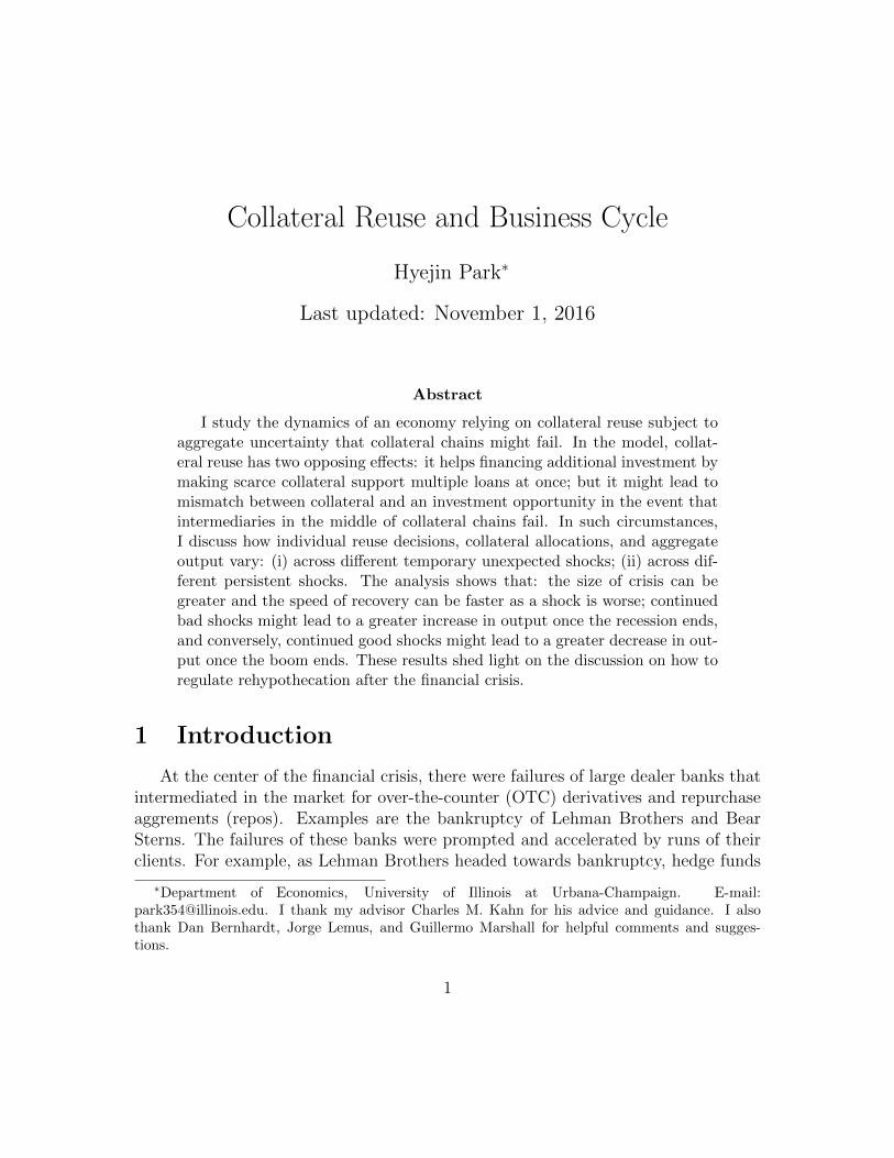
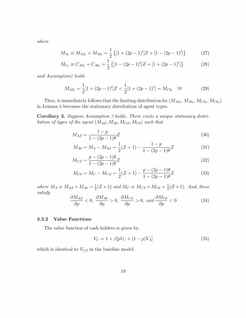
satisfy∂MAZ

∂p< 0,

∂MA0

∂p> 0,

∂MCZ

∂p> 0, and

∂MC0

∂p< 0 (34)

3.3.2 Value Functions

The value function of cash holders is given by,

VC = 1 + β[pVC + (1− p)VA] (35)

which is identical to VCZ in the baseline model.

19

��� ��� ��� ��� ��� ������

���

���

���

���

�

������������������������

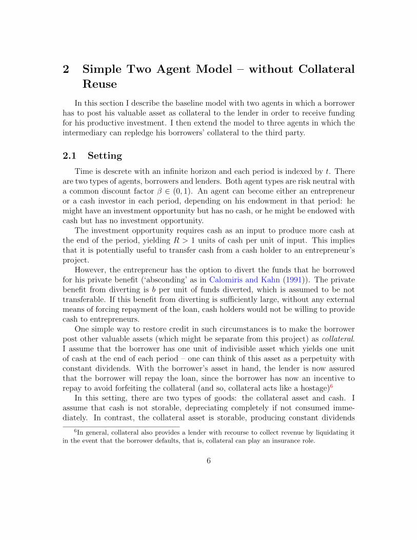
(a) when θ = 0.8 and Z = 1

��� ��� ��� ��� ��� ������

���

���

���

���

θ

������������������������

(b) when p = 0.85 and Z = 1

Figure 1: Comparative Statics of the Steady State Distribution of Types with respectto p (left) and θ (right)

The value function of entrepreneurs is given by,

VA = maxIA,XA

RIA + θ[−XA + {1 + β[pVA + (1− p)VC ]}] (36)

where IA and XA are as in Lemma 5 .Solving these equations (35) and (36) simultaneously reveals that the value func-

tions of entrepreneurs (A) and cash holders (C) take the following forms.

Lemma 7. The value function of enterpreneurs (A) and cash holders (C) are givenby,

VA =γθ[Y − β(2p− 1)]

1− β{p+ γθ[p+ (1− p)(Y − 1)− β(2p− 1)]}(37)

VC =1− γθβ(2p− 1)

1− β{p+ γθ[p+ (1− p)(Y − 1)− β(2p− 1)]}(38)

where γ ≡ b1+b−R > 1.

From this lemma, comparative statics follow immediately.

Corollary 4 (Comparative Statics on the Value Functions).

VA > VC (39)

20

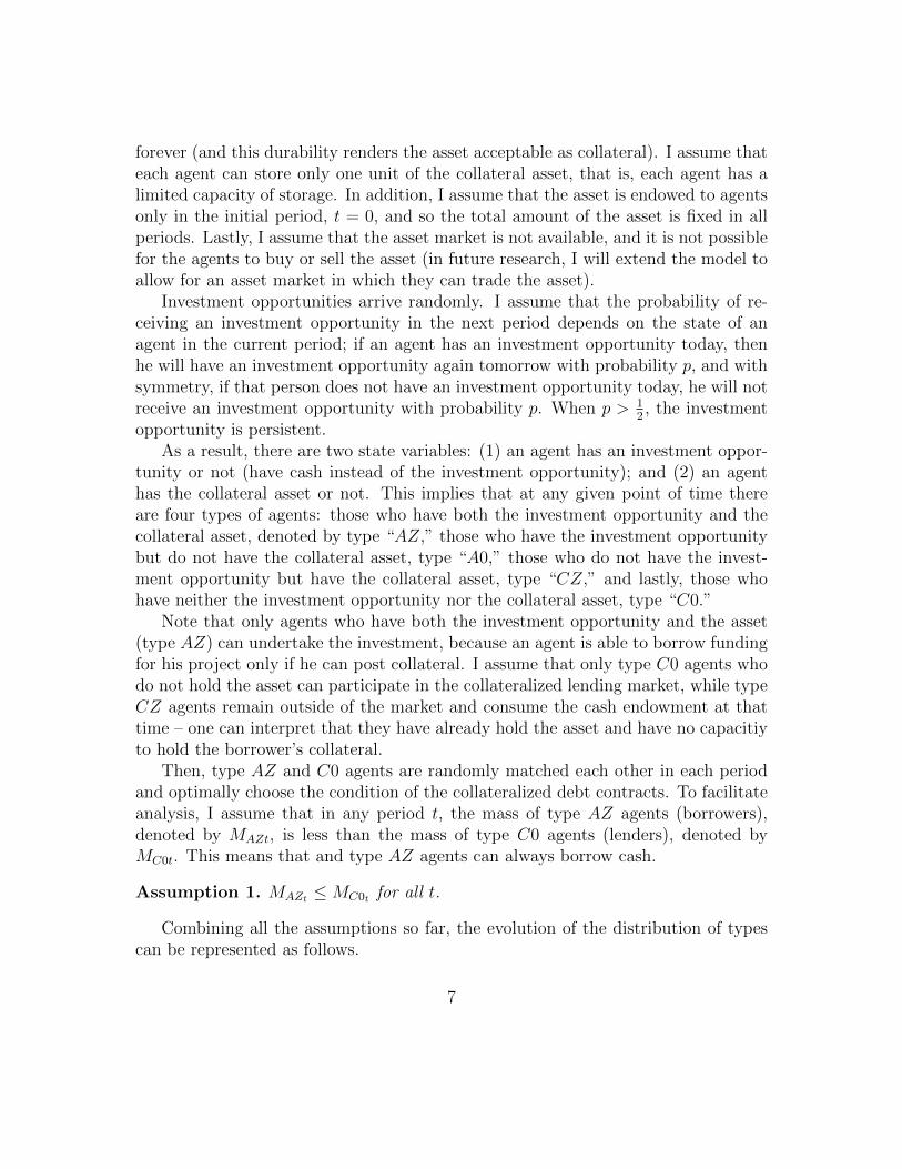
0.5 0.6 0.7 0.8 0.9 1.0

0

5

10

15

20

25

30

35

p

VA,Vc

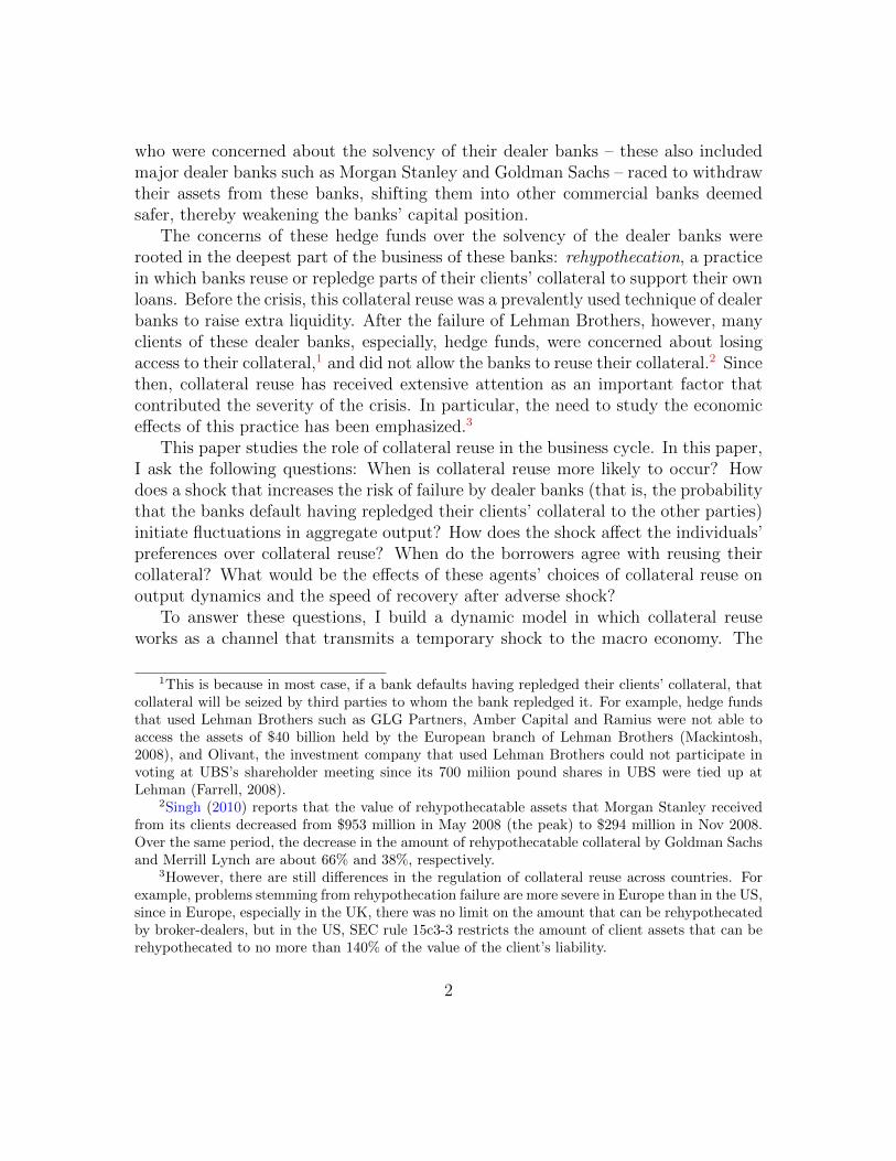
(a) VA and VC when Y < 2− β

0.5 0.6 0.7 0.8 0.9 1.0

2

3

4

5

6

p

VA,Vc

(b) VA and VC when Y > 2− β

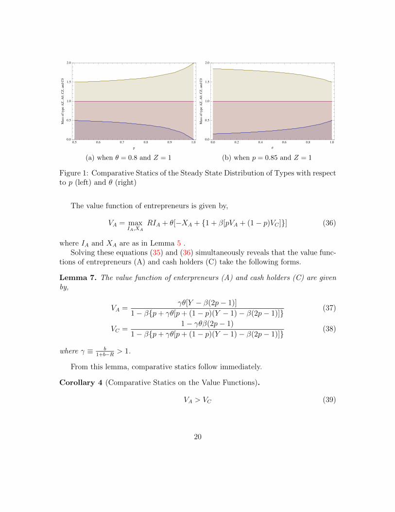
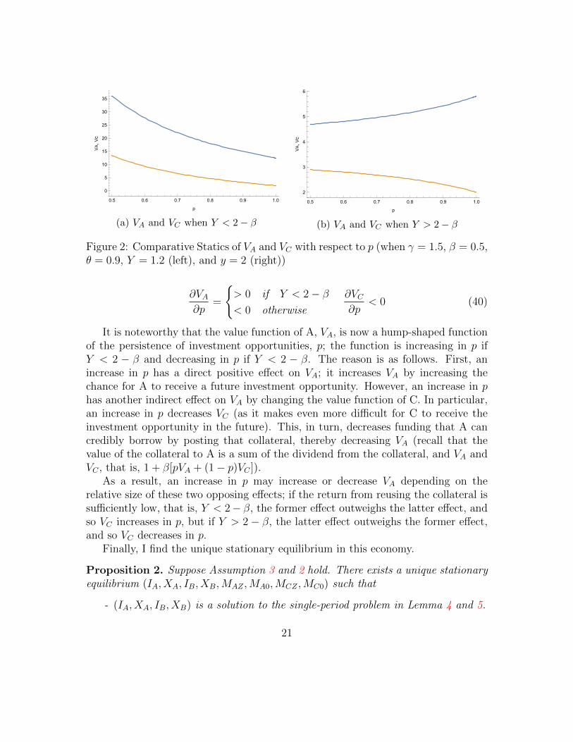
Figure 2: Comparative Statics of VA and VC with respect to p (when γ = 1.5, β = 0.5,θ = 0.9, Y = 1.2 (left), and y = 2 (right))

∂VA∂p

=

{> 0 if Y < 2− β< 0 otherwise

∂VC∂p

< 0 (40)

It is noteworthy that the value function of A, VA, is now a hump-shaped functionof the persistence of investment opportunities, p; the function is increasing in p ifY < 2 − β and decreasing in p if Y < 2 − β. The reason is as follows. First, anincrease in p has a direct positive effect on VA; it increases VA by increasing thechance for A to receive a future investment opportunity. However, an increase in phas another indirect effect on VA by changing the value function of C. In particular,an increase in p decreases VC (as it makes even more difficult for C to receive theinvestment opportunity in the future). This, in turn, decreases funding that A cancredibly borrow by posting that collateral, thereby decreasing VA (recall that thevalue of the collateral to A is a sum of the dividend from the collateral, and VA andVC , that is, 1 + β[pVA + (1− p)VC ]).

As a result, an increase in p may increase or decrease VA depending on therelative size of these two opposing effects; if the return from reusing the collateral issufficiently low, that is, Y < 2− β, the former effect outweighs the latter effect, andso VC increases in p, but if Y > 2− β, the latter effect outweighs the former effect,and so VC decreases in p.

Finally, I find the unique stationary equilibrium in this economy.

Proposition 2. Suppose Assumption 3 and 2 hold. There exists a unique stationaryequilibrium (IA, XA, IB, XB,MAZ ,MA0,MCZ ,MC0) such that

- (IA, XA, IB, XB) is a solution to the single-period problem in Lemma 4 and 5.

21

- (MAZ ,MA0,MCZ ,MC0) is in Corollary 3,

3.4 Choice of Collateral Reuse

Up to this point, I have assumed that B (an intermediary) can always reuse A’scollateral whenever he has an investment opportunity. In practice, however, theborrower (A in this model) has the right to restrict B’s ability to reuse his collateral,and if the risk of losing the collateral and the cost of recovering it are too high,he may want to preclue B’s ability to reuse collateral. I now investigate how theprobability of losing collateral by intermediary B, 1− θ, affects entrepreneur’s (A’s)decisions on whether to allow reusing collateral or not.

Proposition 3. An enterpreneur’s (A’s) decision on whether to allow reusing col-lateral or not depends on the risk of intermediaries’ failure 1− θ as follows:

- he allows collateral reuse if

1− θ < 1− β(2p− 1)

1− β(2p− 1) + (Y − 1)[1− γβ(2p− 1)](41)

and does not allow it, otherwise.

As mentioned earlier, allowing the intermediary (B) to reuse collateral reduces theopportunity costs of keeping the collateral. This, in turn, benefits the enterpreneur(A) since the intermediary now would be willing to provide more funding. Forexample, if the return from the intermediary’s project Y increases, the right handside of Equation 41 increases, and the entrepreneur is more likely to allow collateralreuse. However, allowing the collateral reuse exposes the entrepreneur to the risk oflosing collateral if the intermediary fails. For example, if the probability of defaultsof the intermediary, 1 − θ, increases, the left hand side of Equation 41 increases,and the entrepreneur is less willing to allow collateral reuse. As a result, whether toallow the intermediary to reuse collateral or not depends on the benefits and costsit delivers to the entrepreneur.

4 Dynamics

4.1 The Effect of Temporary Shocks on Output Dynamics

In this section I introduce a shock that increases the risk of default by the in-termediary and investigate its effect on output dynamics. I find that even when

22

magnitudes of shocks are almost the same, the output dynamics triggered by themcan be significantly different depending the agents’ choice over the collateral reuse –whether the borrower continues allowing his counterparty to reuse his collateral ornot in response to the shock.

To be specific, this section addresses the following questions: when does a shockinduce agents to continue to allow the collateral reuse or preclude it?; how does theallocation of collateral change over time in these two cases?; and how does the sizeof the crisis and the speed of recovery differ between these two cases?

It reveals that an adverse shock increases the mismatch between collateral and in-vestment opportunities, decreasing aggregate output. Furthermore, there is anotherindirect effect of the shock on the output dynamics by altering agents’ preferencesover collateral reuse. If the agents continue to allow collateral reuse, the size of thecrisis will be relatively small, but it leads to a long economic downturn by increasingthe mismatch of collateral and investment opportunities in the future. In contrast, ifthe agents discontinue to allow collateral reuse, the size of the crisis will be relativelylarge, but it helps the economy to recover fast by reducing the mismatch of collateraland investment opportunities in the future.

Formally, I begin with a steady-state economy in which collateral reuse is allowedas in Proposition 2.11 Suppose there is a temporary shock that increases the proba-bility of failure of the intermediary in period t; in other words, after the shock, theprobability of success of B’s project falls from θ to (1−∆)θ where ∆ ∈ (0, 1).

Given that the shock is temporary, for a given set of parameters (β, γ, θ, p, Y ), Ican find the range of ∆ in which the borrower allows collateral reuse or not at thetime of the shock.

Lemma 8. Suppose there is a temporary negative shock ∆ in period t. The borrowerallows the collateral reuse in that period only if ∆ satisfies,

(1−∆)θ <1 + β[pVA + (1− p)VC ]

1 + β[pVA + (1− p)VC ] + (Y − 1)VC(42)

where VA and VC are as in Proposition 2.

That is, the borrower will be more cautious to allow collateral reuse as the riskof failure of the intermediary increases, that is, as ∆ increases. It is noteworthy thatthe cutoff in Lemma 8 is different from that in Proposition 3. This is because that

11Dynamics when collateral reuse is not allowed are uninteresting since the collateral is segregatedfrom the counterparty risk, and the aggregate output varies only with the shocks on the borrowers’side.

23

the shock is temporary, and so the value functions VA and VC in this case will remainthe same as in Proposition 2.

The questions is then: how does this borrower’s choice affect the efficient allo-cation of collateral? That is, how does it affect the degree of matching betweencollateral and the investment opportunity? Formally, this can be measured by themass of each type of the agents: an increase in the mass of type AZ implies that morecollateral are associated with the investment opportunity (and vice versa), while anincrease in the mass of type CZ or A0 implies that more collateral and the invest-ment opportunity are mismatched each other. The next proposition illustrates theevolution of the mass of each type of the agents after the shock under these tworegimes.

Proposition 4 (The Allocation of Collateral after the Shock). Suppose there is anagative shock ∆ in period t.

• If ∆ satisfies the condition in Lemma 8, the borrower in period t allows col-lateral reuse, and the mass of each type of the agents in period T ≥ t evolvesaccording to

MAZT = [1−∆(2p− 1)T−tθT−t]MAZ (43)

MA0T =1

2(Z + 1)−MAZT (44)

MCZT = MCZ + ∆(2p− 1)T−tθT−tMAZ (45)

MC0T =1

2(Z + 1)−MCZT (46)

• If ∆ does not satisfy the condition in Lemma 8, the borrower in period t forbidscollateral reuse, and the mass of each type of the agents at T ≥ t evolvesaccording to

MAZT =

{[1 + ∆(2p− 1)(1− θ)]MAZ if T = t+ 1

[1 + ∆(2p− 1)T−tθT−t−1(1− θ)]MAZ if T ≥ t+ 2(47)

MA0T =1

2(Z + 1)−MAZT (48)

MCZT =

{MCZ −∆(2p− 1)(1− θ)MAZ if T = t+ 1

MCZ −∆(2p− 1)T−tθT−t−1(1− θ)MAZ if T ≥ t+ 2(49)

MC0T =1

2(Z + 1)−MCZT (50)

24

where the distribution of types of the agents at t = T is given by the stationarydistribution, (MAZ ,MA0,MCZ ,MC0) as in Proposition 2.

When the borrower continues to allow collateral reuse in period t, the mass oftype AZ in period t+1 falls from its previous steady state level, MAZ , to [1−∆(2p−1)θ]MAZ , but then it starts to increase and converges to its previous steady statelevel as the effect of the shock disappears. At that same time, the mass of type A0and CZ move in the opposite direction of the mass of type AZ.

When the borrower does not allow collateral reuse in period t, however, the massof type AZ in period t+ 1 rises from MAZ to [1 + ∆(2p− 1)(1− θ)]MAZ at t+ 1, butthen it starts to decrease and converges to MAZ as the effect of the shock disappearsand the collateral reuse is allowed again. Similarly, the mass of type A0 and CZmove in the opposite direction of that of type AZ during this period.

To summarize, continuing collateral reuse at the time of the shock increases themismatch between collateral and the investment in the subsequent periods, whilestopping the collateral reuse at the time of the shock decreases it.

Then, the natural question is: what are the implication of the collateral allocation(or misallocation) for output dynamics? And, how does the borrower’s choice overcollateral reuse affect the speed of recovery after the shock?

Proposition 5 (The Output Dynamics after the Shock). Suppose there is a negativeshock ∆ in period t.

• If ∆ satisfies the condition in Lemma 8, the borrower in period t allows collat-eral reuse, and aggregate output in period T ≥ t, denoted by YT , is determinedas follows.

YT =

{[RIA([1−∆]θ) + (1−∆)θY IB([1−∆]θ)]MAZT if T = t

[RIA(θ) + θY IB(θ)]MAZT if T ≥ t+ 1(51)

where IA(·) and IB(·) are as in Lemma 4 and 5, and MAZT is the mass of typeAZ in period T when the collateral reuse is allowed in period t as in Proposition4.

• If ∆ does not satisfy the condition in Lemma 8, the borrower in period t doesnot allow the collateral reuse, and the aggregate output in period T ≥ t isdetermined as follows.

YT =

{RIA(1)MAZT if T = t

[RIA(θ) + θY IB(θ)]MAZT if T ≥ t+ 1(52)

25

where IA(1) is the special case of IA(·) when θ = Y = 1, IA(·) and IB(·) areas in Lemma 4 and 5, and MAZT is the mass of type AZ in period T when thecollateral reuse is not allowed in period t as in Proposition 4.

First, it is noteworthy that the aggregate output is generated from the initialborrower A’s project and the intermediary B’s project: A’s project has a gross returnof RIA and B’s prject has an expected gross return of θY IB, and the mass of typeAZ, MAZ , determines the number of A’s project (and also the number of B’s projectif the collateral is reused).

If the collateral reuse is allowed in period t, the additional project of B is funded,and so the size of crisis will be relatively small, that is, drop in YT will be small–though the funding for A’s project decreases from IA(θ) to IA([1 − ∆]θ) –, butallowing the collateral reuse at the time of the shock has a negative effect to increasethe collateral misallocation in the subsequent periods, that is, decreases MAZT forT ≥ t+ 1, and so the recovery will be slow.

In contrast, if the collateral reuse is not allowed in period t, B’s project cannotbe funded, and so the size of crisis will be relatively large, but discontinuing thecollateral reuse at the time of the shock has a positive effect to increase MAZT forT ≥ t + 1, and so the recovery will be faster compared to the previous case whencontinuing the collateral reuse in period t.

Therefore, Proposition 5 suggests that even magnitudes of shocks are almostthe same, the output dynamics triggered by them might be significantly differentdepending on the borrower’s choice of the collateral reuse at the time of the shock.

4.2 Stochastic Aggregate Shocks

I now consider the possibility that aggregate shocks randomly arrive. I assumethat the counterparty shock θ follows a two-state Markov chain where θ ∈ {θL, θH}with θL ≤ θH and let

πij = Pr(θt+1 = θj|θt = θi) i, j ∈ {H,L}. (53)

That is, πLL and πHH capture the persistence of bad and good states: higher πLLand πHH , greater persistence in bad and good states, respectively. If πLL or πHHequals 1, the state remains to be either θL or θH forever, once reached (and, it boilsdown to the previous case with no persistent aggregate shocks).

26

4.2.1 Equilibrium

As in the previous analysis, in equilibrium, the entrepreneurs’ collateral reusedecision in any period t maximizes expected payoff given a state θt ∈ {θL, θH}, theoptimal single-period contract (IA(θt), Xt(θt), IB(θt), XB(θt)) as in Lemma 4 and 5,and a present value of holding on collateral to the next period,

∑j∈{H,L} πij[pVA(θj)+

(1− p)VC(θj)]. And this determines the evolution of the distribution of types of theagents over time along any path of aggregate shocks (θ1, θ2, . . .). As a result, theequilibrium consists of the optimal decision rule on collateral reuse, the optimalsingle-period contract, the value functions of each type of the agents, and the distri-bution of types of the agents over time that is consistent with the optimization byagents.

First, the value function of entrepreneurs (A) is given by,

VA(θi) ≡ max

{RIA(θi) + θi

[1 + β

∑j∈{H,L}

πij[pVA(θj) + (1− p)VC(θj)]−XA(θi)],

RIA + 1 + β∑

j∈{H,L}

πij[pVA(θj) + (1− p)VC(θj)]− XA

}(54)

where (IA(θi), XA(θi)) are in Proposition 2 and (IA, XA) ≡ (IA(θ = 1, Y = 1), XA(θ =1, Y = 1)). The first term means the value of allowing collateral reuse and the secondterm means the value of not allowing collateral reuse at state θi. This shows thatenterpreneurs choose whether to allow collateral reuse or not to allow it optimally.And the value function of cash holders (C) is given by,

VC(θi) ≡ 1 + β∑

j∈{H,L}

πij[(1− p)VA(θj) + pVC(θj)] (55)

The evolution of the distribution of types that are consistent with the collateralreuse decisions is given by,MAZt+1

MA0t+1

MCZt+1

MC0t+1

=

λt[pθt + (1− p)(1− θt)] + (1− λt)(1− p) 0 1− p 0

λt[(2p− 1)(1− θt)] p 0 1− pλt[(1− p)θt + p(1− θt)] + (1− λt)(1− p) 0 p 0

−λt[(2p− 1)(1− θt)] 1− p 0 p

MAZt

MA0t

MCZt

MC0t

(56)

where θt ∈ {θL, θH}, p ∈(

12, 1]

as in Assumption 2, and λt ∈ {0, 1} where λt = 1means that collateral reuse is allowed and λt = 0 means that collateral reuse is not

27

allowed.If πLL or πHH equals 1, the state θL or θH is absorbing in the sense that it is

never left once reached.12 Then, with the state constant over time, the mass ofentrepreneurs with collateral, MAZ , converges to either (1−p)Z

1−θH(2p−1)or Z

2(where Z is

the initial endowment of collateral), the mass of enterpreneurs with collateral inducedby an arbitrarily long sequence of θ = θH and θ = θL, respectively – by assumptionabove, if θ = θL, collateral reuse does not occur, so that MAZ is independent of θ.

Let M{θτ}tτ=0AZt

(MAZ0) denote the mass of entrepreneurs with collateral t periodsafter following sequence of states {θτ}tτ=0, starting from the mass MAZ0 . Then itleads to the following lemma immediately.

Lemma 9. Suppose Assumption 3 holds. For θ ∈ {θL, θH}, if collateral reuse isallowed only when θ = θH , then,

(i) The interval[

(1−p)Z1−θH(2p−1)

, Z2

]is absorbing in the sense that given any initial

MAZ0 ∈[

(1−p)Z1−θH(2p−1)

, Z2

], for any sequence of states {θτ}tτ=0, M

{θτ}tτ=0AZt

(MAZ0) ∈[(1−p)Z

1−θH(2p−1), Z

2

](ii) For any MAZ0 /∈

[(1−p)Z

1−θH(2p−1), Z

2

],

limt→∞

Prob

({{θτ}tτ=0

∣∣∣∣M{θτ}tτ=0AZt

(MAZ0) ∈[

(1− p)Z1− θH(2p− 1)

,Z

2

]})= 1

4.2.2 Effects of Prolonged Shocks on Output Dynamics

Here, I focus on the case in which enterpreneurs allows collateral reuse if θ = θHand do not allow it if θ = θL, that is, the decision on collateral reuse depends onthe state of the economy. I study the impact of persistence of aggregate shocks –that is, either good (θH) or bad (θL) states continues for a long time – on the outputdynamics.

Specifically, I contrast the output dynamics in two economies that start from thesame state, but one is followed by a prolonged period of good states (θH , θH , . . . , θH)and another is followed by a prolonged period of bad states, (θL, θL, . . . , θL). Theanalysis is complicated by the fact that adverse shocks θL reduce the incentive forentrepreneurs to allow collateral reuse which decreases funding provided to the in-vestment opportunities. However, the persistence of adverse shocks may also raise

12The analysis here closely follows Bergin and Bernhardt (2008).

28

the future outputs since not allowing collateral reuse mitigates the misallocationof collateral, in other words, decreases the mismatch of collateral and investmentopportunities.

I characterize the evolution of the distribution of types of the agents and theaggregate output when a shock θ persists for a long period of time.

Proposition 6. For θ ∈ {θL, θH} and for MAZt−1 ∈[

(1−p)Z1−θ(2p−1)

, Z2

],

1. If θt−1 = θH , so that collateral reuse occurs in period t− 1;

(i) If a good shock arrives in period t, θt = θH , and continues until t + τ ,then the mass of entrepreneurs with collateral (type AZ) falls throughout,MAZt−1 > MAZt > . . . > MAZt+τ , so that aggregate output falls throughout:Yt−1 > Yt > Yt+1 > . . . > Yt+τ .

(ii) If a bad shock arrives in period t , θt = θL, and continues until t+ τ , thenMAZt−1 > MAZt < MAZt+1 < . . . < MAZt+τ , so that aggregate output firstfalls and then rises: Yt−1 > Yt < Yt+1 < . . . < Yt+τ .

2. If θt−1 = θL, so that collateral reuse does not occur in period t− 1;

(i) If θt = θH , and continues until t+τ , then MAZt−1 < MAZt > . . . > MAZt+τ ,so that aggregate output first rises and then falls: Yt−1 < Yt > Yt+1 > . . . >Yt+τ .

(ii) If θt = θL, and continues until t + τ , then MAZt−1 < MAZt < MAZt+1 <. . . < MAZt+τ , so that aggregate output rises throughout: Yt−1 < Yt <Yt+1 < . . . < Yt+τ .

This result shows that, with two aggregate shocks, {θL, θH}, a prolonged period ofgood states increases misallocation between collateral and investment opportunities(that is, increases MAZ), which, in turn, decreases output during the period of goodstates (as in 1-(i) and 2-(i) above). In contrast, a prolonged period of bad statesdecreases misallocation between collateral and investment opportunities, leading toa growth in output during the period of bad states (as in 1-(ii) and 2-(ii) above).It is noteworthy that this result also offers an empirical prediction that economieswith a longer history of downturn has a better allocation of collateral, and thus willproduce greater output, once the economy has recovered.

29

5 Numerical Examples

I assume that the economy is initially at the steady state described in Proposition2. I set the discount rate β = 0.5. The other paraters are R = 1, b = 2 (and so,γ ≡ b

1+b−R = 1), Y = 2, θ = 0.95 (that is, the probability that the intermediarymight default is 5 percent), and Z = 0.9 (the total endowment of the collateral assetis less than the endowment of cash at any given point of time, that is, collateral isscarce).

Then I check that these parameters are consistent with the incentives of theagents. First, parameters satify the condition in Proposition 3, and so the borrowerallows collateral reuse in the steady state. Second, the parameters satisfy the ex postparticipation condition for the intermediary; θ[(Y − 1)VC +XA] > XA where the lefthand size is the expected profit if the intermediary reuses collateral and the righthand side is that if he does not reuse the collateral and just holds on to it. In otherwords, the parameters guarantee that the intemediary wants to reuse collateral expost.

In period 3 I introduce temporary negative shocks ∆ that decrease the probabilityof success of the intermediary from θ to (1 − ∆)θ, and study the evolution of themass of agent types and the aggregate output dynamics after the shock. I select∆ = 0.35 and ∆ = 0.36 to make the sizes of these shocks as similar as possible.

When the size of the shock is ∆ = 0.35, the decrease in the probability of successof the intermediary is relatively small, and the parameters still satisfy the condition inProposition 3, implying that the borrower allows collateral reuse even after the shock.When the size of the shock is ∆ = 0.36, however, the decrease in the probability ofsuccess of the intermediary is relatively large, and the parameters no longer satisfythe condition in Proposition 3, implying that the borrower does not allow collateralreuse after the shock. Lastly, in both cases, the intermediary wants to reuse collateralex post, i.e., θ[(Y − 1)VC +XA] > XA holds for both ∆ = 0.35 and ∆ = 0.36.

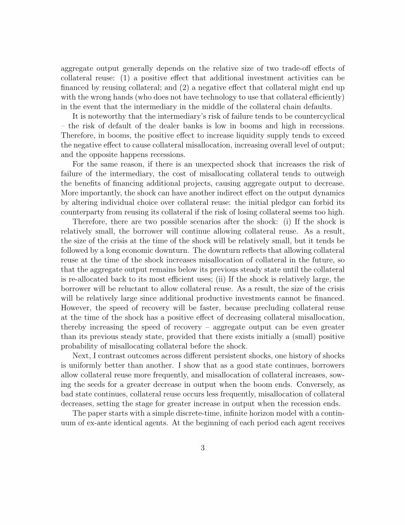
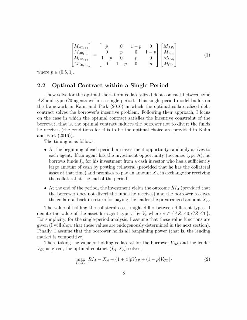
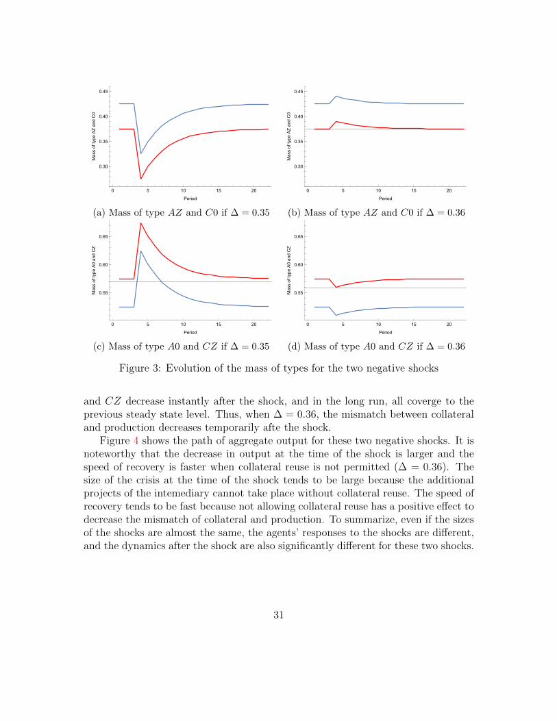
Figure 3 illustrates the evolution of distribution of types of the agents for thesetwo negative shocks. When ∆ = 0.35, as shown in Proposition 4, due to continuingcollateral reuse at the time of the shock, the mass of type AZ and C0 decreasesinstantly, but in the long run, both converge to the previous steady state level sincethe shock is temporary. On the other hand, the mass of type A0 and CZ increasesinstantly, but in the long run, both also converge to the steady state level. Thus, when∆ = 0.35, the mismatch between collateral and production increases temporarilyafter the shock.

In contrast, when ∆ = 0.36, the borrower forbids collateral reuse at the time ofthe shock, and the mass of type AZ and C0 increase, while the mass of type A0

30

0 5 10 15 20

0.30

0.35

0.40

0.45

Period

MassoftypeAZandC0

(a) Mass of type AZ and C0 if ∆ = 0.35

0 5 10 15 20

0.30

0.35

0.40

0.45

Period

MassoftypeAZandC0

(b) Mass of type AZ and C0 if ∆ = 0.36

0 5 10 15 20

0.55

0.60

0.65

Period

MassoftypeA0andCZ

(c) Mass of type A0 and CZ if ∆ = 0.35

0 5 10 15 20

0.55

0.60

0.65

Period

MassoftypeA0andCZ

(d) Mass of type A0 and CZ if ∆ = 0.36

Figure 3: Evolution of the mass of types for the two negative shocks

and CZ decrease instantly after the shock, and in the long run, all coverge to theprevious steady state level. Thus, when ∆ = 0.36, the mismatch between collateraland production decreases temporarily afte the shock.

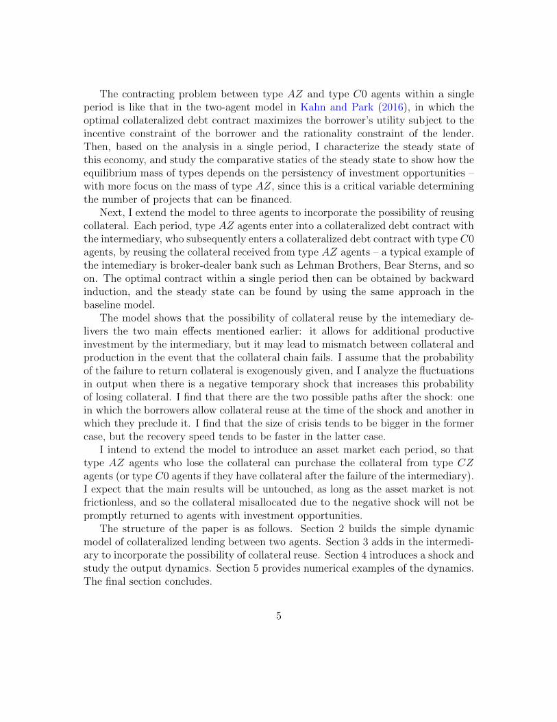
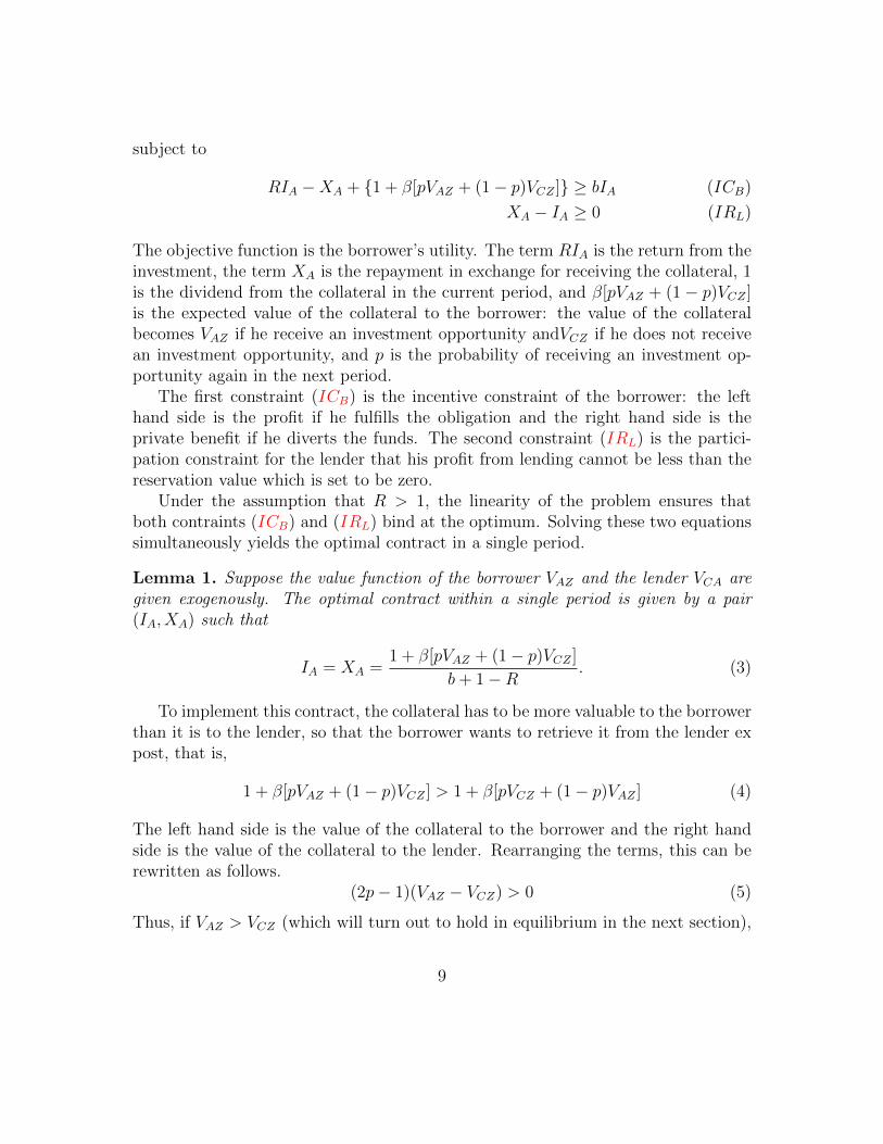
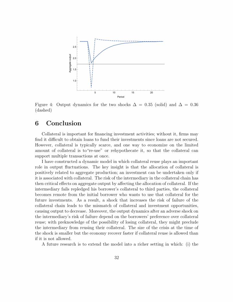
Figure 4 shows the path of aggregate output for these two negative shocks. It isnoteworthy that the decrease in output at the time of the shock is larger and thespeed of recovery is faster when collateral reuse is not permitted (∆ = 0.36). Thesize of the crisis at the time of the shock tends to be large because the additionalprojects of the intemediary cannot take place without collateral reuse. The speed ofrecovery tends to be fast because not allowing collateral reuse has a positive effect todecrease the mismatch of collateral and production. To summarize, even if the sizesof the shocks are almost the same, the agents’ responses to the shocks are different,and the dynamics after the shock are also significantly different for these two shocks.

31

5 10 15 20

1.0

1.5

2.0

2.5

Period

Aggregateoutput

Figure 4: Output dynamics for the two shocks ∆ = 0.35 (solid) and ∆ = 0.36(dashed)

6 Conclusion

Collateral is important for financing investment activities; without it, firms mayfind it difficult to obtain loans to fund their investments since loans are not secured.However, collateral is typically scarce, and one way to economize on the limitedamount of collateral is to“re-use” or rehypothecate it, so that the collateral cansupport multiple transactions at once.

I have constructed a dynamic model in which collateral reuse plays an importantrole in output fluctuations. The key insight is that the allocation of collateral ispositively related to aggregate production; an investment can be undertaken only ifit is associated with collateral. The risk of the intermediary in the collateral chain hasthen critical effects on aggregate output by affecting the allocation of collateral. If theintermediary fails repledged his borrower’s collateral to third parties, the collateralbecomes remote from the initial borrower who wants to use that collateral for thefuture investments. As a result, a shock that increases the risk of failure of thecollateral chain leads to the mismatch of collateral and investment opportunities,causing output to decrease. Moreover, the output dynamics after an adverse shock onthe intermediary’s risk of failure depend on the borrowers’ preference over collateralreuse; with preknowledge of the possibility of losing collateral, they might precludethe intermediary from reusing their collateral. The size of the crisis at the time ofthe shock is smaller but the economy recover faster if collateral reuse is allowed thanif it is not allowed.

A future research is to extend the model into a richer setting in which: (i) the

32

borrowers have heterogeneous preferences of holding collateral, and so the choices ofallowing collateral reuse might differ across the borrowers; (ii) the asset market isavailable, and the borrower who lose collateral can repurchase it from the market,but as long as the asset market has frictions the misallocation of collateral if thecollateral chain fails will have a prolonged effect on output.

A Proofs

Proof of Corollary 2. Lemma 3 implies that

VAZ − VCZ =γ − 1

1− β{p+ γ[p− β(2p− 1)]}> 0

since γ ≡ b1+b−R > 1.

Similarly, Lemma 3 implies that

∂VAZ∂p

=γβ(1− β)(γ − 1)

(1− β{p+ γ[p− β(2p− 1)]})2> 0

and∂VCZ∂p

=−β(1− βγ)(γ − 1)

(1− β{p+ γ[p− β(2p− 1)]})2< 0

Proof of Corollary 4. From Lemma 7, one can show

VA − VC =γθY − 1

1− β{p+ γθ[p+ (1− p)(Y − 1)− β(2p− 1)]}> 0

since γθY > 1.Similarly, using Lemma 3, one can show

∂VA∂p

=γβ(2− β − Y )(γθY − 1)

(1− β{p+ γθ[p+ (1− p)(Y − 1)− β(2p− 1)]})2=

{> 0 if Y < 2− β< 0 otherwise

and∂VC∂p

=−β(1− βγθ)(γθY − 1)

(1− β{p+ γθ[p+ (1− p)(Y − 1)− β(2p− 1)]})2< 0

33

Proof of Lemma 6. First, note that the mass of type A and C, that is, MAt ≡MAZt+MA0t and MCt ≡MCZt +MC0t follows a first order Markov chain,[

MAt+1

MCt+1

]=

[p 1− p

1− p p

] [MAt

MCt

](57)

This implies that

MAt =1

2

{[1 + (2p− 1)t]MA0 + [1− (2p− 1)t]MC0

}(58)

MCt =1

2

{[1− (2p− 1)t]MA0 + [1 + (2p− 1)t]MC0

}(59)

Second, provided that MAZt ≤MC0t for all t, the mass of type AZ, A0, CZ, andC0 evolves over time as follows,

MAZt+1

MA0t+1

MCZt+1

MC0t+1

=

pθ + (1− p)(1− θ) 0 1− p 0

(2p− 1)(1− θ) p 0 1− p(1− p)θ + p(1− θ) 0 p 0−(2p− 1)(1− θ) 1− p 0 p

MAZt

MA0t

MCZt

MC0t

(60)

Rearranging the terms and using the fact that MAZt + MCZt ≡ MAZ0 + MCZ0 ,the equations can be written as functions of the initial distributions, MAt , MCt , andMAZt only;

MAZt+1 = (1− p)(MAZ0 +MCZ0) + (2p− 1)θMAZt (61)

MA0t+1 = pMAt + (1− p)MCt − [(1− p)(MAZ0 +MCZ0) + (2p− 1)θMAZt ] (62)

MCZt+1 = p(MAZ0 +MCZ0)− (2p− 1)θMAZt (63)

MC0t+1 = (1− p)MAt + pMCt − [p(MAZ0 +MCZ0)− (2p− 1)θMAZt ] (64)

where

MAZt = (1− p)[

1− (2p− 1)tθt

1− (2p− 1)θ

](MAZ0 +MCZ0) + (2p− 1)tθtZ (65)

MAt =1

2

{[1 + (2p− 1)t]MA0 + [1− (2p− 1)t]MC0

}(66)

MCt =1

2

{[1− (2p− 1)t]MA0 + [1 + (2p− 1)t]MC0

}(67)

Lastly, I want to show that MAZt ≤ MC0t for all t. I begin to show that this

34

holds for t = 1. By Assumption 3,

MAZ1 = (1− p)(MAZ0 +MCZ0) + (2p− 1)θMAZ0

MC01 = (1− p)MA0 + pMC0 − [p(MAZ0 +MCZ0)− (2p− 1)θMAZ0 ]

implying,

MC01 −MAZ1 = (1− p)MA0 + pMC0 − (MAZ0 +MCZ0)

=1

2[MA00 +MC00 − (MAZ0 +MCZ0)]

+

(p− 1

2

)[MC00 +MCZ0 − (MA00 +MAZ0)]

≥ 0

where the inequality holds by Assumption 2 and 3.Next, I want to show that if MAZt ≤ MC0t holds, MAZt+1 ≤ MC0t+1 also holds.

Since MAZt ≤MC0t ,

MAZt+1 = (1− p)(MAZ0 +MCZ0) + (2p− 1)θMAZt

MC0t+1 = (1− p)MAt + pMCt − [p(MAZ0 +MCZ0)− (2p− 1)θMAZt ]

implying,

MC0t+1 −MAZt+1 = (1− p)MAt + pMCt − (MAZ0 +MCZ0)

= (1− p)1

2

{[1 + (2p− 1)t]MA0 + [1− (2p− 1)t]MC0

}+ p

1

2

{[1− (2p− 1)t]MA0 + [1 + (2p− 1)t]MC0

}− (MAZ0 +MCZ0)

=1

2[1− (2p− 1)t+1]MA0 +

1

2[1 + (2p− 1)t+1]MC0 − (MAZ0 +MCZ0)

=1

2[MA00 +MC00 − (MAZ0 +MCZ0)] +

1

2(2p− 1)t+1(MC0 −MA0)

≥ 0

where the inequality is by Assumption 2 and 3.

35

B Heterogeneity in Cost of Losing Collateral

I now relax the assumption that all collateral yield the same fixed dividend. Sup-pose collateral may yields a random dividend, h ∈ [1, h] where F (h) is distributionfunction of h. I assume that h (which will be realized at the end of a period) isknown to owners of the collateral (and also to the intermediary if the owners borrowfunds against the collateral13) at the beginning of the period. Here, h represents thedifferences in costs of losing collateral; if h is large, the collatearal owner would beunwilling to allow collateral reuse since he cannot collect h if it is lost, and for thesimilar reason, if h is small, he would be willing to allow collateral reuse.

To characterize the equilibrium in such case, I begin with the single period prob-lem as before. Taking h as given, optimal contract (IA, XA) between the entrepreneur(A) and the intermediary (B) solves

maxIA,XA

RIA + θ{h+ β[pVA + (1− p)VC ]−XA} (68)

subject to

RIA + θ{h+ β[pVA + (1− p)VC ]−XA} ≥ bIA (ICAh)

θ(Y IB −XB +XA) ≥ IA (IRBh)

The objective function is the entrepreneur’s payoff from undertaking the projectwith collateralized borrowing as before, when dividend of collateral is h. Constraint(ICAh) and (IRBh) is the incentive constraint of the entrepreneur and the partici-pation constraint of the intermediary, respectively. In particular, constraint (IRBh)can be rewritten,

θ(Y IB −XB +XA) = θ(Y − 1)VC + θXA ≥ IA (IRBh)

where the equality follows from that the optimal contract between the intermediary(B) and the cash holder (C) satisfies14

IB = XB = VC ≡∫ h

1

hdF (h) + β[(1− p)VA + pVC ].

13One may think that the intermediary can evaluate the value of the underlying collateral.14Again, I assume that C does not know h nor the contract terms between A and B.

36

Then, the optimal contract (IA(h), XA(h)) is given by,

IA(h) = θh+ β[pVA + (1− p)VC ] + (Y − 1)VC

1 + b−R(69)

XA(h) =h+ β[pVA + (1− p)VC ] + (b−R)(Y − 1)VC

1 + b−R(70)

and the expected utility of entrepreneur (when collateral is reused) is given by,

UA(h) ≡ RIA(h) + θ{h+ β[pVA + (1− p)VC ]−XA(h)}. (71)

In addition, the entrepreneur chooses whether to allow collateral reuse or not bycomparing this to the utility if he does not allow collateral reuse. And, the utilitywhen collateral is not reused can be computed by substituting θ = 1 and Y = 1 toUA(h) above,

UA(h) ≡ RIA(h; θ = 1, Y = 1)+θ{h+β[pVA+(1−p)VC ]−XA(h; θ = 1, Y = 1)} (72)

Comparing the utility UA(h) and UA(h) yields the cutoff h∗ at which the en-trepreneur is indifferent between allowing collateral reuse and not allowing it.

h∗ =θ

1− θ(Y − 1)VC − β[pVA + (1− p)VC ]. (73)

And the value fuction of the entrepreneur VA and that of the cash holder VC aregiven by,

VA ≡∫ h∗

1

U(h)dF (h) +

∫ h

h∗U(h)dF (h) (74)

= γ

{θ

∫ h∗

1

hdF (h) +

∫ h

h∗hdF (h) + β[θF (h∗) + 1− F (h∗)][pVA + (1− p)VC ]

(75)

+ θF (h∗)(Y − 1)VC

}(76)

VC ≡∫ h

1

hdF (h) + β[(1− p)VA + pVC ] (77)

In summary, the value functions VA and VC are the solutions to the followingsystem of equations.

37

Lemma 10. Suppose h is a random variable distributed over the interval [1, h], witha distribution function F . The value functions VA and VC satisfy,

VA = γ

{θ

∫ θ1−θ (Y−1)VC−β[pVA+(1−p)VC ]

1

hdF (h) +

∫ h

θ1−θ (Y−1)VC−β[pVA+(1−p)VC ]

hdF (h)

(78)

+ β

[1− (1− θ)F

(θ

1− θ(Y − 1)VC − β[pVA + (1− p)VC ]

)][pVA + (1− p)VC ]

(79)

+ θF

(θ

1− θ(Y − 1)VC − β[pVA + (1− p)VC ]

)(Y − 1)VC

}(80)

VC =

∫ h

1

hdF (h) + β[(1− p)VA + pVC ] (81)

Next, I solve for a stationary distribution of types. I assume that the initialdistribution satisfies Assumption 3.

Note that type AZ agents allow collateral reuse only if h < h∗ = θ1−θ (Y − 1)VC −

β[pVA + (1− p)VC ]. If Assumption 1 holds, the mass of each type then evolves overtime as follows.MAZt+1

MA0t+1

MCZt+1

MC0t+1

=

p[1− (1− θ)F (h∗)] + (1− p)(1− θ)F (h∗) 0 1− p 0

(2p− 1)(1− θ)F (h∗) p 0 (1− p)(1− p)[1− (1− θ)F (h∗)] + p(1− θ)F (h∗) 0 p 0

−(2p− 1)(1− θ)F (h∗) 1− p 0 p

MAZt

MA0t

MCZt

MC0t

(82)

References

Andolfatto, D., Martin, F. M., and Zhang, S. (2015). Rehypothecation and liquidity.FRB St Louis Paper No. FEDLWP2015-003.

Bergin, J. and Bernhardt, D. (2008). Industry dynamics with stochastic demand.The RAND Journal of Economics, 39(1):41–68.

Bernanke, B. and Gertler, M. (1989). Agency costs, net worth, and business fluctu-ations. The American Economic Review, pages 14–31.

38

Biais, B., Heider, F., and Hoerova, M. (2015). Risk-sharing or risk-taking? counter-party risk, incentives and margins. Journal of Finance, Forthcoming.

Bolton, P. and Oehmke, M. (2015). Should derivatives be privileged in bankruptcy?The Journal of Finance, 70(6):2353–2394.

Bottazzi, J.-M., Luque, J., and Pascoa, M. R. (2012). Securities market theory:Possession, repo and rehypothecation. Journal of Economic Theory, 147(2):477–500.

Brunnermeier, M. K. and Pedersen, L. H. (2009). Market liquidity and fundingliquidity. Review of Financial studies, 22(6):2201–2238.

Calomiris, C. W. and Kahn, C. M. (1991). The role of demandable debt in structuringoptimal banking arrangements. The American Economic Review, pages 497–513.

Duffie, D., Scheicher, M., and Vuillemey, G. (2015). Central clearing and collateraldemand. Journal of Financial Economics, 116(2):237–256.

Eren, E. (2014). Intermediary funding liquidity and rehypothecation as determinantsof repo haircuts and interest rates. In 27th Australasian Finance and BankingConference.

Geanakoplos, J. (2010). The leverage cycle. In NBER Macroeconomics Annual 2009,Volume 24, pages 1–65. University of Chicago Press.

Gertler, M., Kiyotaki, N., et al. (2010). Financial intermediation and credit policyin business cycle analysis. Handbook of monetary economics, 3(3):547–599.

Gertler, M., Kiyotaki, N., and Queralto, A. (2012). Financial crises, bank risk expo-sure and government financial policy. Journal of Monetary Economics, 59:S17–S34.

Gorton, G. and Metrick, A. (2012). Securitized banking and the run on repo. Journalof Financial economics, 104(3):425–451.

Gorton, G. and Ordonez, G. (2014). Collateral crises. The American EconomicReview, 104(2):343–378.

Greenwood, R. M., Hanson, S. G., and Stein, J. C. (2010). A comparative-advantageapproach to government debt maturity. Harvard Business School Finance WorkingPaper, (1680604).

39

Holmstrom, B. and Tirole, J. (1996). Private and public supply of liquidity. Technicalreport, National Bureau of Economic Research.

Holmstrom, B. and Tirole, J. (2011). Inside and outside liquidity. MIT press.

Infante, S. (2014). Money for nothing: The consequences of repo rehypothecation.Available at SSRN, (2460979).

Kahn, C. M. and Park, H. (2016). Collateral, rehypothecation, and efficiency. UIUCWorking Paper.

Kiyotaki, N. and Moore, J. (1995). Credit cycles. Technical report, National Bureauof Economic Research.

Krishnamurthy, A. and Vissing-Jorgensen, A. (2013). Short-term debt and financialcrises: What we can learn from us treasury supply. unpublished, NorthwesternUniversity, May.

Lee, J. (2015). Collateral circulation and repo spreads. Available at SSRN 2548209.

Mills, D. C. and Reed, R. R. (2008). Default risk and collateral in the absence ofcommitment. Available at SSRN 1148963.

Mills, Jr., D. C. and Reed, R. R. (2012). Default risk and collateral in the absenceof commitment. manuscript.

Monnet, C. (2011). Rehypothecation. Business Review, Federal Reserve Bank ofPhiladelphia, (Q4):18–25.

Moore, J. (2011). Leverage stacks and the financial system. Ross Prize Lecture.

Muley, A. (2016). Collateral reuse in shadow banking and monetary policy. MITWorking Paper.

Singh, M. (2010). The sizable role of rehypothecation in the shadow banking system.IMF Working Papers.

Singh, M. (2011). Velocity of pledged collateral: analysis and implications. IMFWorking Papers, pages 1–24.

Singh, M. (2014). Collateral and Financial Plumbing. Risk Books.

40