Collateral Equilibrium∗

John Geanakoplos William R. Zame

Yale University UCLA

Abstract Much of the lending in modern economies is secured by some form

of collateral: residential and commercial mortgages and corporate bonds are

familiar examples. This paper builds an extension of general equilibrium

theory that incorporates durable goods, collateralized securities and the pos-

sibility of default to argue that the reliance on collateral to secure loans and

the particular collateral requirements chosen by the social planner or by

the market have a profound impact on prices, allocations, the structure of

markets, and the efficiency of market outcomes. These findings provide in-

sights into housing and mortgage markets, including the sub-prime mortgage

market.

August 29, 2010

∗Earlier versions of this paper circulated under the titles “Collateral, Default and Market Crashes”

and “Collateral and the Enforcement of Intertemporal Contracts.” We thank Pradeep Dubey and

seminar audiences at British Columbia, Caltech, Harvard, Illinois, Iowa, Minnesota, Penn State,

Pittsburgh, Rochester, Stanford, UC Berkeley, UCLA, USC, Washington University in St. Louis, the

NBER Conference Seminar on General Equilibrium Theory and the Stanford Institute for Theoreti-

cal Economics for comments. Financial support was provided by the Cowles Foundation (Geanako-

plos), the John Simon Guggenheim Memorial Foundation (Zame), the UCLA Academic Senate

1 Introduction

Recent events in financial markets provide a sharp reminder that much of the lending

in modern economies is secured by some form of collateral: residential and commercial

mortgages are secured by the mortgaged property itself, corporate bonds are secured

by the physical assets of the firm, collateralized mortgage obligations and debt obli-

gations and other similar instruments are secured by pools of loans that are in turn

secured by physical property. The total of such collateralized lending is enormous: in

2007, the value of U.S. residential mortgages alone was roughly $10 trillion and the

(notional) value of collateralized credit default swaps was estimated to exceed $50

trillion. The reliance on collateral to secure loans is so familiar that it might be easy

to forget that it is a relatively recent innovation: extra-economic penalties such as

debtor’s prisons, indentured servitude, and even execution were in widespread use in

Western societies into the middle of the 19th Century.

Reliance on collateral to secure loans — rather than on extra-economic penalties

— avoids the moral and ethical issues of imposing penalties in the event of bad luck,

the cost of imposing penalties, and the difficulty of finding the defaulter in order to

impose penalties at all. Penalties represent a pure deadweight loss: to the borrower

who defaults, to the lender who suffers the default, and to society as a whole. The

reliance on collateral, which simply transfers resources from one owner to another,

is intended to avoid this deadweight loss.1 This paper argues, however, that the

reliance on collateral – and the particular levels of collateral chosen (by the planner

or by the market) – have a profound effect on prices, on allocations, on the structure

of financial institutions, and especially on the efficiency of market outcomes. In

particular collateral requirements limit both borrowing and lending and distort both

Committee on Research (Zame), and the National Science Foundation (Geanakoplos, Zame). Any

opinions, findings, and conclusions or recommendations expressed in this material are those of the

authors and do not necessarily reflect the views of any funding agency.1In practice, seizure of collateral may involve deadweight losses of its own.

choices and prices. Moreover, although lower collateral requirements make it easier to

borrow to buy goods they also increase competition between borrowers for the very

same goods

To make these points, we formulate an extension of intertemporal general equilib-

rium theory that incorporates durable goods, collateral and the possibility of default.

To focus the discussion, we restrict attention to a pure exchange framework with

two dates but many possible states of nature (representing the uncertainty at time

0 about exogenous shocks at time 1). As is usual in general equilibrium theory, we

view individuals as anonymous price-takers; for simplicity, we use a framework with

a finite number of agents and divisible loans.2

Central to the model is that the definition of a security must now include not just

its promised deliveries but also the collateral required to back that promise; the same

promise backed by a different collateral constitutes a different security and might

trade at a different price. We assume that collateral is held and used by the borrower

and that forfeiture of collateral is the only consequence of default; in particular, there

are no penalties for default other than forfeiture of the collateral, and there is no

destruction of property in the seizure of collateral. As a result, borrowers will always

deliver the minimum of what is promised and the value of the collateral. Lenders,

knowing this, need not worry about the identity of the borrowers but only about the

value of the collateral. Our model requires that each security be collateralized by

a distinct bundle of physical goods; residential mortgages (in the absence of second

liens) provide the canonical example of such securities.

2Anonymity and price-taking might appear strange in an environment in which individuals might

default. In our context, however, individuals will default when the value of promises exceeds the

value of collateral and not otherwise; thus lenders do not care about the identity of borrowers,

but only about the collateral they bring. The assumption of price-taking might be made more

convincing by building a model that incorporates a continuum of individuals, and the realism of the

model might be enhanced by allowing for indivisible loans, but doing so would complicate the model

without qualitatively changing the conclusions.

2

Although default is suggestive of disequilibrium, our model passes the basic test

of consistency: under the hypotheses on agent behavior and foresight that are stan-

dard in the general equilibrium literature, equilibrium always exists (Theorem 1).

The existence of equilibrium rests on the fact that collateral requirements place an

endogenous bound on short sales. (The reader will recall that it is the possibility

of unbounded short sales that leads to non-existence of equilibrium in the standard

model of general equilibrium with incomplete markets.)

The familiar models of Walrasian equilibrium (WE) and of general equilibrium with

incomplete markets (GEI) tacitly assume that all agents keep all their promises, but

ignore the question of why agents should keep their promises; implicitly the familiar

models assume that there are infinite penalties for breaking promises – so that agents

always keep their promises and always make promises that they will be able to keep.

We compare collateral equilibrium (CE) to Walrasian equilibrium and to general

equilibrium with incomplete markets as a way of seeing how equilibrium changes

when we make the opposite assumption: that borrowers have no incentive to repay

beyond the desire to retain the collateral and that the only recourse for the lender is

to confiscate the collateral. Modulo some assumptions we find that whenever CE is is

not equivalent to GEI there are distortions in security prices and commodity prices,

which can be identified as a liquidity wedge and a collateral value (Theorem 2), and

that whenever CE is not equivalent to WE it is Pareto suboptimal. (Theorem 3).

These ideas are introduced in a simple mortgage market (Example 1) in which CE

is surprisingly complicated. We compute collateral equilibrium as a function of the

wealth distribution and collateral requirements and identify parameter regions where

CE is Pareto optimal and coincident with WE and GEI and parameter regions where

it is not; in the latter regions we identify distortions. We also show that the welfare

impact of collateral requirements is ambiguous: lower collateral requirements make

it possible for buyers to hold more houses but create more competition for the same

3

houses, thereby driving up the prices.3

Adding uncertainty to our simple mortgage market (Examples 2, 3) allows us to

make a number of additional points. A striking point is that collateral requirements

that lead to default (with positive probability) in equilibrium may (ex ante) Pareto

dominate collateral requirements that do not lead to default. Moreover, if securities

offering the same promise but backed by different collateral requirements are offered,

the market may choose a collateral requirement that leads to default (with posi-

tive probability). This suggests an important implication for the subprime mortgage

market that seems to have been ignored: even if it is true that defaults on subprime

mortgages led to a crash ex post, such mortgages might have been Pareto improving

ex ante. Finally, even if all possible securities are offered, only a few may be actively

traded; in particular, the market may be endogenously incomplete. Whether the mar-

ket always chooses efficient collateral requirements - or more generally, an efficient

set of securities – or whether it can sometimes be welfare improving for government

to restrict collateral requirements or security offerings is a question to which we do

not have an answer. We do show, however, that government action can improve

social welfare only if it alters terminal prices (Theorem 4). Hence any valid welfare-

based argument for regulation of down-payment requirements would seem to require

that regulators can correctly forecast the price changes that would accompany such

regulation.

3This seems relevant to a complete understanding of U.S. housing and mortgage markets over

the last hundred years. Before World War I, mortgage down payment requirements were typically

on the order of 50%. The rise of Savings and Loan institutions, later the VHA and FHA – and

most recently the sub-prime mortgage market – have all made it easier for (some) consumers to

obtain mortgages with much lower down payment requirements. Lower down payment requirements

increase competition and drive up housing prices, so some (perhaps very substantial) portion of

the boom in housing prices may have over this period should presumably be ascribed to these

institutional changes in mortgage markets, rather than to a change in fundamentals. (Contrast

Mankiw and Weil (1989).)

4

When all lending must be collateralized, the supply of collateral becomes an im-

portant financial constraint. If collateral is in short supply the necessity of using

collateral to back promises creates incentives to create collateral and to stretch ex-

isting collateral. The state can (effectively) create collateral by issuing bonds that

can be used as collateral and by promulgating law and regulation that make it easier

to seize goods used as collateral.4,5 The market’s attempts to stretch collateral have

driven much of the financial engineering that has rapidly accelerated over the last

three-and-a-half decades (beginning with the introduction of mortgage-backed secu-

rities in the early 1970’s) and that has been designed specifically to stretch collateral

by making it possible for the same collateral to be used several times: allowing agents

to collateralize their promises with other agents’ promises (pyramiding) and allowing

the same collateral to back many different promises (tranching). These two innova-

tions are at the bottom of the securitization and derivatives boom on Wall Street,

and have greatly expanded the scope of financial markets. We address these issues in

a companion paper Geanakoplos and Zame (2010).

Following a brief discussion of related literature (below), Section 2 presents the

model and Section 3 presents the existence theorem (Theorem 1). Our simple mort-

gage market (Example 1) is presented in Section 4. Section 5 identifies (Theorem 2)

the distortion when collateral equilibrium differs from GEI as arising from a liquidity

4The home mortgage market in Israel provides an interesting example. Historically, government

regulation made it easy to seize owner-occupied homes on which the mortgage was in default,

but difficult to seize renter-occupied homes, providing an incentive for owners near default to rent

their homes to close relatives at below-market prices. As a consequence of the difficulty of seizure,

down payment requirements frequently exceeded 50% of the sale price and mortgages were difficult

to obtain. In the 1980’s, changes in government regulations made it easier to seize renter-occupied

homes. As a consequence, down payment requirements fell to levels comparable to the U.S. mortgage

market and mortgages became much easier to obtain.

5Similarly, state regulations concerning seizure can have an enormous influence on bankruptcies;

see Lin and White (2001) and Fay, Hurst, and White (2002) for instance.

5

wedge and collateral value. Section 6 shows that efficient collateral equilibrium is

Walrasian (Theorem 3). Section 7 adds uncertainty to the simple mortgage market

(Examples 2, 3) to show that both the social planner and the market may choose

collateral requirements that lead to default and that, at least in some circumstances,

the market chooses efficiently (Theorem 4). Section 8 concludes. The (long) proof of

Theorem 1 (existence) is relegated to the Appendix.

Literature

Hellwig (1981) provides the first theoretical treatment of collateral and default in

a market setting; the focus of that work is on the extent to which the Modigliani–

Miller irrelevance theorem survives the possibility of default. Dubey, Geanakoplos,

and Zame (1995), Geanakoplos (1997) and Geanakoplos and Zame (1997, 2002) (the

last of which are forerunners of the present work), provide the first general treatments

of a market in which deliveries on financial securities are guaranteed by collateral re-

quirements. Araujo, Pascoa, and Torres-Martinez (2002) use a version of the same

model to show that collateral requirements rule out the possibility of Ponzi schemes

in infinite-horizon models, and hence eliminate the need for the transversality require-

ments that are frequently imposed (Magill and Quinzii, 1994; Hernandez and Santos,

1996; Levine and Zame, 1996). Araujo, Fajardo, and Pascoa (2005) expand the model

to allow borrowers to set their own collateral levels, and Steinert and Torres-Martinez

(2007) expand the model to accommodate security pools and tranching.

Dubey, Geanakoplos, and Shubik (2005) is a seminal work in a somewhat different

literature, which treats extra-economic penalties for default. (In that particular pa-

per, extra-economic penalties are modeled as direct utility penalties; when penalties

are sufficiently severe, that model reduces to the standard model in which enforcement

is perfect — and costless, because penalties are never imposed in equilibrium). One of

the central points of that paper, and of Zame (1993), which uses a very similar model,

6

is that the possibility of default may promote efficiency (a point that is made here, in

a different way, in Example 2). Kehoe and Levine (1993) builds a model in which the

consequences of default are exclusion from trade in subsequent financial markets, but

these penalties constrain borrowing in such a way that there is no equilibrium default.

Sabarwal (2003) builds a model which combines many of these features: securities

are collateralized, but the consequences of default may involve seizure of other goods,

exclusion from subsequent financial markets and extra-economic penalties, as well as

forfeiture of collateral. Kau, Keenan, and Kim (1994) provide a dynamic model of

mortgages as options, but ignore the general equilibrium interrelationship between

mortgages and housing prices.

Bernanke, Gertler, and Gilchrist (1996) and Holmstrom and Tirole (1997) are sem-

inal works in a quite different literature that focuses on asymmetric information be-

tween borrowers and lenders as the source of borrowing limits.

A substantial empirical literature examines the effect of bankruptcy and default

rules (especially with respect to mortgage markets) on consumption patterns and

security prices. Lin and White (2001), Fay, Hurst, and White (2002), Lustig and

Nieuwerburgh (2005) and Girardi, Shapiro, and Willen (2008) are closest to the

present work.

2 Model

As in the canonical model of securities trading, we consider a world with two dates;

agents know the present but face an uncertain future. At date 0 (the present) agents

trade a finite set of commodities and securities. Between date 0 and date 1 (the

future) the state of nature is revealed. At date 1 securities pay off and commodities

are traded again.

7

2.1 Time & Uncertainty

There are two dates 0 and 1, and S possible states of nature at date 1. We frequently

refer to 0, 1, . . . , S as spots.

2.2 Commodities, Spot Markets & Prices

There are L ≥ 1 commodities available for consumption and trade in spot markets

at each date and state of nature; the commodity space is RL(1+S) = RL × RLS. A

bundle x ∈ RL(1+S) is a claim to consumption at each date and state of the world. For

x ∈ RL(1+S) and indices s, `, xs is the bundle specified by x in sport s and xs` is the

quantity of commodity ` specified in spot s. We write δs` ∈ RL for the commodity

bundle consisting of one unit of commodity ` in spot s and nothing else. If x ∈ RL+

then (x, 0) ∈ RL(1+S) is the bundle in which x is consumed at date 0 and nothing is

consumed at date 1. Similarly, if (x1, . . . , xS) ∈ RLS then (0, (x1, . . . , xS)) ∈ RL(1+S)

is the bundle in which xs is consumed in state s and nothing is consumed at date 0.

We write x ≥ y to mean that xs` ≥ ys` for each s, `; x > y to mean that x ≥ y and

x 6= y; and x� y to mean that xs` > ys` for each s, `.

We depart from the usual intertemporal models by allowing for the possibility that

goods are durable. If x0 ∈ RL is consumed (used) at date 0 we write Fs(x0) for what

remains in state s at date 1. We assume the map F : S×RL → RL is continuous and

is linear and positive in consumption. The commodity 0` is perishable if F (δ0`) ≡ 0

and durable otherwise. It may be helpful to think of F as being analogous to a

production function – except that inputs to production can also be consumed.

For each s, there is a spot market for consumption at spot s. Prices at each spot

lie in RL++, so RL(1+S)

++ is the space of spot price vectors. For p ∈ RL(1+S), ps is the

vector of prices in spot s and ps` is the price of commodity ` in spot s.

8

2.3 Consumers

There are I consumers (or types of consumers). Consumer i is described by a con-

sumption set, which we take to be RL(1+S)+ , an endowment ei ∈ RL(1+S)

+ , and a utility

function ui : RL(1+S)+ → R.

2.4 Collateralized Securities

A collateralized security (security for short) is a pair A = (A, c); A : S×RL(1+S)++ → R+

is a continuous function, the promise or face value (denominated in units of account)

and c ∈ RL+ is the collateral requirement. In principle, the promise in state s may

depend on prices ps in state s and prices p0 at date 0 and even on prices ps′ in other

states. The collateral requirement c is a bundle of date 0 commodities; an agent

wishing to sell one share of (A, c) must hold the commodity bundle c. (Recall that

selling a security is borrowing.)

In our framework, the collateral requirement is the only means of enforcing promises.6

Hence, if agents optimize, the delivery per share of security (A, c) in state s will not

be the face value As(p) but rather the minimum of the face value and the value of

the collateral in state s:

Del((A, c), s, p) = min{As(p), ps · Fs(c)}

The delivery on a portfolio θ = (θ1, . . . , θJ) ∈ RJ is

Del(θ, s, p) =∑

j

θjDel((Aj, cj); s, p)

We take as given a family of J securities A = {(Aj, cj)}. (The number J of

securities might be very large.) Because deliveries never exceed the value of collateral,

we assume without loss of generality that Fs(cj) 6= 0 for some s. (Securities that fail

this requirement will deliver nothing; in equilibrium the price of such securities will

6Loans with this property are frequently called no recourse loans.

9

be 0 and trade in such securities will be irrelevant.) It is notationally convenient to

distinguish between security purchases and sales; we typically write ϕ, ψ ∈ RJ+ for

portfolios of security purchases and sales, respectively.7 We assume that buying and

selling prices for securities are identical; we write q ∈ RJ+ for the vector of security

prices. An agent who sells the portfolio ψ ∈ RJ+ will have to hold (and will enjoy) the

collateral bundle Coll(ψ) =∑ψjcj.

Our formulation allows for nominal securities, for real securities, for options and for

complicated derivatives. For ease of exposition, our examples focus on real securities.

2.5 The Economy

An economy (with collateralized securities) is a tuple E = 〈(ei, ui),A〉, where (ei, ui) is

a finite family of consumers and A = {(Aj, cj)} is a family of collateralized securities.

(The set of commodities and the durable goods technology are fixed, so are suppressed

in the notation.) Write e =∑ei for the social endowment. The following assumptions

are always in force:

• Assumption 1 e+ (0, F (e0)) � 0

• Assumption 2 For each consumer i: ei > 0

• Assumption 3 For each consumer i:

(a) ui is continuous and quasi-concave

(b) if x ≥ y ≥ 0 then ui(x) ≥ ui(y)

(c) if x ≥ y ≥ 0 and xs` > ys` for some s 6= 0 and some `, then ui(x) > ui(y)

(d) if x ≥ y ≥ 0, x0` > y0`, and commodity 0` is perishable, then ui(x) > ui(y)

The first assumption says that all goods are represented in the aggregate (keeping in

mind that some date 1 goods may only come into being when date 0 goods are used).

7In principle, agents might go long and short in the same security, although in the present

framework there is no reason why they should do so.

10

The second assumption says that individual endowments are non-zero. The third as-

sumption says that utility functions are continuous, quasi-concave, weakly monotone,

strictly monotone in date 1 consumption of all goods and in date 0 consumption of

perishable goods.8

2.6 Budget Sets

Given a set of securities A, commodity prices p and security prices q, a consumer with

endowment e must make plans for consumption, for security purchases and sales, and

for deliveries against promises. In view of our earlier comments, we assume that

deliveries are precisely the minimum of promises and the value of collateral, so we

suppress the choice of deliveries. We therefore define the budget set B(p, q, e,A) to

be the set of plans (x, ϕ, ψ) that satisfy the budget constraints at date 0 and in each

state at date 1 and the collateral constraint at date 0:

• at date 0

p0 · x0 + q · ϕ ≤ p0 · e0 + q · ψ

x0 ≥ Coll(ψ)

In words: expenditures for date 0 consumption and security purchases do not

exceed income from endowment and from security sales, and date 0 consumption

includes collateral for all security sales.

• in state s

ps · xs + Del(ψ, s, p) ≤ ps · es + ps · Fs(x0) + Del(ϕ, s, p)

In words: expenditures for state s consumption and for deliveries on promises do

not exceed income from endowment, from the return on date 0 durable goods,

and from collections on others’ promises.

8We do not require strict monotonicity in durable date 0 goods because we want to allow for

the possibility that claims to date 1 consumption are traded at date 0; of course, such claims would

typically provide no utility at date 0.

11

If these conditions are satisfied, we frequently say that the portfolio (ϕ, ψ) finances

x at prices p, q.9

Note that if security promises in each state depend only on commodity prices in

that state and are homogeneous of degree 1 in those commodity prices – in particular,

if securities are real (promise delivery of the value of some commodity bundle) –

then budget constraints depend only on relative prices. In general, however, budget

constraints may depend on price levels as well as on relative prices.

2.7 Collateral Equilibrium

A collateral equilibrium for the economy E = 〈(ei, ui),A〉 consists of commodity prices

p ∈ RL(1+S)++ , security prices q ∈ RJ

+ and consumer plans (xi, ϕi, ψi) satisfying the usual

conditions:

• Commodity Markets Clear 10

∑xi =

∑ei +

∑F (ei

0)

• Security Markets Clear ∑ϕi =

∑ψi

• Plans are Budget Feasible

(xi, ϕi, ψi) ∈ B(p, q; ei,A)

• Consumers Optimize

(x, ϕ, ψ) ∈ B(p, q, ei,A) ⇒ ui(x) ≤ ui(xi)9Agents know date 0 prices but must forecast date 1 prices. Our equilibrium notion implicitly

incorporates the requirement that forecasts be correct, so we take the familiar shortcut of suppressing

forecasts and treating all prices as known to agents at date 0. See Barrett (2000) for a model in

which forecasts might be incorrect.

10As in a production economy, the market clearing condition for commodities incorporates the

fact that some date 1 commodities come into being from date 0 activities.

12

2.8 Walrasian Equilibrium

As noted in the Introduction, it is useful to compare/contrast collateral equilibrium

(CE) with Walrasian equilibrium (WE) and general equilibrium with incomplete mar-

kets (GEI). Here and in the next subsection we record the formalizations of the lat-

ter notions in the present durable goods framework. Throughout, we maintain a

fixed structure of commodities and preferences: in particular, date 0 commodities are

durable and Fs(x0) is what remains in state s if the bundle x0 is consumed at date 0.

A durable goods economy is a family 〈(ei, ui)〉 of consumers, specified by endow-

ments and utility functions. We use notation in which a purchase at date 0 conveys

the rights to what remains at date 1; hence if commodity prices are p ∈ R(1+S)L++ , the

Walrasian budget set for a consumer whose endowment is e is

BW (e, p) = {x ∈ RL(1+S)+ : p · x ≤ p · e+ p · (0, F (x0))}

A Walrasian equilibrium consists of commodity prices p and consumption choices xi

such that

• Commodity Markets Clear∑xi =

∑ei +

∑(0, F (ei

0))

• Plans are Budget Feasible

xi ∈ BW (ei, p)

• Consumers Optimize

yi ∈ BW (ei, p) ⇒ ui(yi) ≤ ui(xi)

2.9 GEI

In the familiar GEI model, as in our collateral model, goods are traded on spot

markets but only securities are traded on intertemporal markets. In the GEI context

13

a security is a claim to units of account at each future state s as a function of prices;

D : S × RL(1+S) × RL → R. A GEI economy is a tuple 〈(ei, ui), {Dj}〉 of consumers

and securities.

To maintain the parallel with our collateral framework, we keep security purchases

and sales separate. Given commodity spot prices p ∈ RL(1+S)++ and security prices

q ∈ RJ , the budget set BGEI(p, q, e, {Dj}) for a consumer with endowment e consists

of plans (x, ϕ, ψ) (x ∈ RL(1+S)+ is a consumption bundle; ϕ, ψ ∈ RJ

+ are portfolios of

security purchases and sales, respectively) that satisfy the budget constraints at date

0 and in each state at date 1:

• at date 0

p0 · x0 + q · ϕ ≤ p0 · e0 + q · ψ

• in state s

ps · xs +∑

j

ψjDjs(p) ≤ ps · es + ps · (0, Fs(x0)) +

∑j

ϕjDjs(p)

Note that the GEI budget set differs from the collateral budget set in that there is

no collateral requirement at date 0 and security deliveries coincide with promises.

A GEI equilibrium consists of commodity spot prices p ∈ RL(1+S)++ , security prices

q ∈ RJ , and plans (xi, ϕi, ψi) such that:

• Commodity Markets Clear∑xi =

∑ei +

∑F (ei

0)

• Security Markets Clear ∑ϕi =

∑ψi

• Plans are Budget Feasible

(xi, ϕi, ψi) ∈ B(ei, p, q, {Dj})

14

• Consumers Optimize

(x, φ, ψ) ∈ B(ei, p, q, {Dj}) ⇒ ui(x) ≤ ui(xi)

3 Existence of Collateral Equilibrium

Under the maintained assumptions discussed in Section 2, collateral equilibrium al-

ways exists; we relegate the (long) proof to the Appendix.

Theorem 1 (Existence) Under the maintained assumptions, every economy admits

a collateral equilibrium.

This may seem a surprising result, because we allow for real securities, options,

derivatives and even more complicated non-linear securities; in the standard model of

incomplete financial markets, the presence of any of these securities may be incom-

patible with existence of equilibrium.11 In our framework, however, the requirement

that security sales be collateralized places an endogenous bound on short sales. As

in Radner (1972), a bound on short sales eliminates the discontinuity in budget sets

that gives rise to non-existence and thus guarantees the existence of equilibrium.12

4 Price Distortion: Collateral Value, Liquidity Wedge

As we will show, if CE does not reduce to GEI then some CE prices must deviate

from what they would be in GEI, and in a particular way. We identify the deviation

in commodity prices as a “collateral value” and the deviation in security prices as a

“liquidity wedge”.

11See Hart (1975) for the seminal example of non-existence of equilibrium with real securities,

Duffie and Shafer (1985) and Duffie and Shafer (1986) for generic existence with real securities, and

Ku and Polemarchakis (1990) for robust examples of non-existence of equilibrium with options.

12Araujo, Pascoa, and Torres-Martinez (2002) exploit a similar idea to show that collateral re-

quirements rule out Ponzi schemes in markets with an infinite horizon.

15

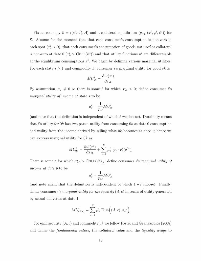
Fix an economy E = 〈(ei, ui),A〉 and a collateral equilibrium 〈p, q, (xi, ϕi, ψi)〉 for

E . Assume for the moment that that each consumer’s consumption is non-zero in

each spot (xis > 0), that each consumer’s consumption of goods not used as collateral

is non-zero at date 0 (xi0 > Coll(ψi)) and that utility functions ui are differentiable

at the equilibrium consumptions xi. We begin by defining various marginal utilities.

For each state s ≥ 1 and commodity k, consumer i’s marginal utility for good sk is

MU isk =

∂ui(xi)

∂xsk

By assumption, xs 6= 0 so there is some ` for which xis` > 0; define consumer i’s

marginal utility of income at state s to be

µis =

1

ps`

MU is`

(and note that this definition is independent of which ` we choose). Durability means

that i’s utility for 0k has two parts: utility from consuming 0k at date 0 consumption

and utility from the income derived by selling what 0k becomes at date 1; hence we

can express marginal utility for 0k as:

MU i0k =

∂ui(xi)

∂x0k

+S∑

s=1

µis [ps · Fs(δ

0k)]

There is some ` for which xi0` > Coll(ψi)0`; define consumer i’s marginal utility of

income at date 0 to be

µi0 =

1

p0`

MU i0`

(and note again that the definition is independent of which ` we choose). Finally,

define consumer i’s marginal utility for the security (A, c) in terms of utility generated

by actual deliveries at date 1

MU i(A,c) =

S∑s=1

µis Del

((A, c), s, p

)For each security (A, c) and commodity 0k we follow Fostel and Geanakoplos (2008)

and define the fundamental values, the collateral value and the liquidity wedge to

16

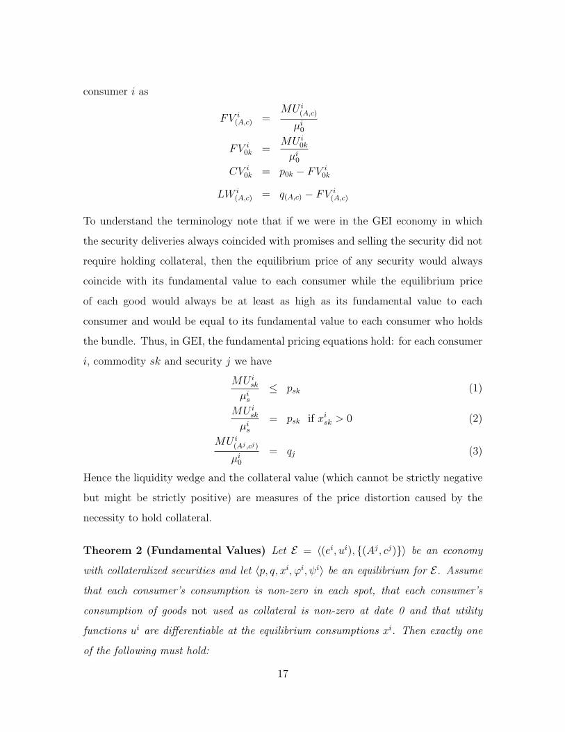
consumer i as

FV i(A,c) =

MU i(A,c)

µi0

FV i0k =

MU i0k

µi0

CV i0k = p0k − FV i

0k

LW i(A,c) = q(A,c) − FV i

(A,c)

To understand the terminology note that if we were in the GEI economy in which

the security deliveries always coincided with promises and selling the security did not

require holding collateral, then the equilibrium price of any security would always

coincide with its fundamental value to each consumer while the equilibrium price

of each good would always be at least as high as its fundamental value to each

consumer and would be equal to its fundamental value to each consumer who holds

the bundle. Thus, in GEI, the fundamental pricing equations hold: for each consumer

i, commodity sk and security j we have

MU isk

µis

≤ psk (1)

MU isk

µis

= psk if xisk > 0 (2)

MU i(Aj ,cj)

µi0

= qj (3)

Hence the liquidity wedge and the collateral value (which cannot be strictly negative

but might be strictly positive) are measures of the price distortion caused by the

necessity to hold collateral.

Theorem 2 (Fundamental Values) Let E = 〈(ei, ui), {(Aj, cj)}〉 be an economy

with collateralized securities and let 〈p, q, xi, ϕi, ψi〉 be an equilibrium for E. Assume

that each consumer’s consumption is non-zero in each spot, that each consumer’s

consumption of goods not used as collateral is non-zero at date 0 and that utility

functions ui are differentiable at the equilibrium consumptions xi. Then exactly one

of the following must hold:

17

(i) Fundamental value pricing holds and the CE is a GEI: each consumer finds

that all date 0 commodities he holds and all securities are priced at their fun-

damental values and 〈p, q, xi, ϕi, ψi〉 is a GEI for the incomplete markets econ-

omy 〈(ei, ui), {Dj}〉 (where Dj is the security whose deliveries are Dj(s, p) =

Del((Aj, cj), s, p)); or

(ii) Fundamental value pricing fails and the CE is not a GEI: some consumer i

finds a strictly positive liquidity wedge for some security (Aj, cj) and also finds

a strictly positive collateral value for some good 0k for which cj0k > 0. If in

addition consumer i sells (Aj, cj) then fundamental values pricing fails for both

security (Aj, cj) and the good 0k.

Proof As we have noted, the budget and market-clearing conditions for CE imply

those for GEI. Because utility functions are quasi-concave, in order that the given

CE reduce to GEI it is thus necessary and sufficient that the fundamental pricing

equations (1), (2), (3) hold for each consumer i, commodity sk and security j. If the

given CE does not reduce to GEI then at least one of these equations must fail; we

must show that the failure(s) are of the type(s) specified.

Note that the left hand sides of the fundamental pricing equations (1), (2), (3)

are just what we have defined as the fundamental values. Because any agent can

always consume less of some good that she does not use as collateral and use the

additional income to buy more of any good or of any security, both commodity prices

and security prices must weakly exceed fundamental value for every agent.

Now consider a security (Aj, cj) that is sold at equilibrium and some agent i who

sells it. Agent i can always reduce or increase all his holding of the collateral bundle

cj and the amount ψij of the security that he sells by a common common infinitesi-

mal fraction ε without violating the collateral constraints, moving the resulting rev-

enue into or out of consumption that is not used as collateral. Because the agent

is optimizing at equilibrium, this marginal move must yield zero marginal utility.

18

Keeping in mind that µi0 is agent i’s marginal utility for income at date 0 yields

MU icj −MU i(Aj ,cj) = µi

0(p · cj − qj), and dividing by µi0 yields

FV icj − FV i

(Aj ,cj) = p · cj − qj

Rearranging yields

p · cj − FV icj = qj − FV i

(Aj ,cj)

As we have already noted, commodity prices are always weakly above fundamental

values, so p · cj > FV icj exactly when p0k > FV i

0k for some commodity 0k for which

cj0k > 0. We conclude that agent i finds a liquidity wedge for the security (Aj, cj) he

sells if and only if he finds a collateral value for some commodity that is part of the

collateral cj. The price for each good an agent consumes but does not use entirely

as collateral in date 0 or consumes in any spot at date 1 must equal its fundamental

value to him. Hence if no agent i is selling a security with a liquidity wedge, then

every good is priced at its fundamental value to every agent who holds it.

If there do not exist a security (Aj, cj) and agent i who sells (Aj, cj) and finds

both a liquidity wedge and collateral value, the only remaining distortion possibility

is that there is some security (Aj′ , cj′) that is not sold at equilibrium and some agent

i who finds a liquidity wedge for (Aj′ , cj′). Agent i could have increased his sales of

the security while buying the necessary collateral. Hence there must be a collateral

value to him of some good in cj′(which he might not be holding in equilibrium). This

completes the proof.

Theorem 2 may seem at odds with Kiyotaki and Moore (1997), who show that

prices of collateral goods may be below fundamental values. However, Kiyotaki and

Moore (1997) do not make the natural assumption that we have made: that date 0

consumptions include goods not pledged as collateral.

19

4.1 Collateral Value and Efficient Markets

Theorem 2 tells us that, at a collateral equilibrium, there are two possibilities. The

first is that no agent would choose to sell more of any security if s/he did not have to

put up the collateral (but were still committed to the same deliveries), then collateral

equilibrium reduces to GEI (with appropriately defined securities payoffs). In that

situation, the collateral requirement does not lead to a different equilibrium than

GEI – but it does play the important role of endogenizing security payoffs. The

second is that if some agent would choose to sell more of any security if s/he did not

have to put up the collateral (but were still committed to the same deliveries). then

collateral equilibrium does not reduce to GEI and fundamental value pricing fails for

at least one agent and one security; moreover, if the agent is selling that security,

then fundamental value pricing fails for at least one durable good as well.

The latter conclusion contradicts the standard efficient markets hypothesis of asset

pricing. In particular, durable assets – houses or companies – that yield exactly the

same payoffs can trade at different prices if one is more easily used as collateral. This

seems an especially important point in a setting in which some investors are unin-

formed or unsophisticated. A central implication of the efficient markets hypothesis

is that, in equilibrium, prices “level the playing field” for uninformed/unsophisticated

investors: it is not necessary for investors to know or understand everything about an

asset because everything relevant will be revealed by its price. However, as Theorem

2 shows, if an uninformed/unsophisticated investor buys some asset – a house or a

company – that has a high collateral value, trusting that it is priced correctly by

the market and hence will yield the usual risk adjusted expected return, then that

investor might be sadly disappointed if he does not leverage his purchase by taking

out a big loan against the house.

20

4.2 Collateral Value and Endogenous Securities

How does the scarcity of collateral manifest itself in equilibrium? If collateral is the

only reason for delivery, then the aggregate value of promises traded cannot exceed the

aggregate value of collateral – but the desired level of promises might be much higher.

How, in equilibrium, are agents (collectively) restrained from making more promises?

(As long as agents are consuming positive amounts of food in equilibrium, any one of

them could borrow more by buying collateral and using it to back a promise.) The

answer is that collateral must be held at a price exceeding its fundamental value. A

promise will not be traded if its liquidity wedge is smaller than the corresponding

collateral value. And this collateral value tends to limit the amount an agent wants

to sell of any promise, because the more he sells, the more collateral he must hold, so

the smaller the liquidity wedge becomes and the higher the collateral value becomes

(assuming fixed prices and diminishing marginal utility).

As in Geanakoplos (1997), the scarcity of collateral rations promises, and thus

endogenizes securities payoffs – beyond its role in default. Potential loans must com-

pete for the same collateral and loans with small liquidity wedges relative to collateral

value will not be traded in equilibrium at all – even though they are available and

priced by the market. For example, an Arrow security (that promises delivery in only

one state) might provide large gains to trade (in the sense that its liquidity wedge

may be large relative to its price) but have a small market price if there are many

states in which the promised delivery is zero, so that the liquidity wedge it provides

is smaller still. In that circumstance, a bigger promise might create a bigger liquidity

wedge, using the same collateral, and thus completely choke off trade in the Arrow

security. Example 3 in Section 7 illustrates just this point (among others).

21

5 A Simple Mortgage Market

In this section we offer a simple example that illustrates the working of our model and

some of the points described in the Introduction, and suggests some of the general

results that follow.

Example 1 [A Mortgage Market] Consider a world with no uncertainty (S = 1).

There are two goods at each date: food F which is perishable and housing H which

is perfectly durable. There are two consumers (or two types of consumers, in equal

numbers); endowments and utilities are:

e1 = (18− w, 1; 9, 0) u1 = x0F + x0H + x1F + x1H

e2 = (w, 0; 9, 0) u2 = log x0F + 4x0H + x1F + 4x1H

We take w ∈ (0, 18) as a parameter. (Consumer 1 finds food and housing to be

perfect substitutes and has constant marginal utility of consumption; Consumer 2

finds date 0 housing and date 1 housing to be perfect substitutes, likes housing more

than Consumer 1, but has decreasing marginal utility for date 0 food.)

As a benchmark, we begin by recording the unique Walrasian equilibrium 〈p, x〉

(leaving the simple calculations to the reader). If we normalize so that p0F = 1 then

equilibrium prices , consumptions and utilities are:

p0F = 1 , p1F = 1 , p0H = 8 , p1H = 4

x1 = (17, 0; 18− w, 0) u1 = 35− w

x2 = (1, 1;w, 1) u2 = 8 + w

(Consumer 2 likes housing much more than Consumer 1 and is rich in date 1, so,

whatever her date 0 endowment, she buys all the date 0 housing – borrowing from

her date 1 endowment if necessary, and of course repaying if she does so.) Note that

individual equilibrium utilities depend on w, but total utility is always 43 – which is

the level it must be at any Pareto efficient allocation in which both agents consume

22

food in date 1. (Both agents have constant marginal utility of 1 for date 1 food, so

utility is transferable in the range where both consume date 1 food.)

In the GEI world, in which securities always deliver precisely what they promise

and security sales do not need to be collateralized, the Walrasian outcome will again

obtain when there are at least as many independent securities as states of nature –

here, at least one security whose payoff is never 0.

However, in the world of collateralized securities, no agent can make guarantees

to pay without offering collateral, and Walrasian outcomes need not obtain. To the

extent Consumer 2 can use housing as collateral, she will be able to buy more housing

with borrowed money. However, competition will then raise the price of housing. We

can trace out the effects of these opposite forces across the range of security promises

(equivalently, collateral requirements).

We assume that only one security (Aα, c) = (αp1F , δ0H) is available for trade; (Aα, c)

promises the value of α units of food in date 1 and is collateralized by 1 unit of date

0 housing.13 We take w ∈ (0, 18) and α ∈ [0, 4] as parameters. (As we shall show,

p1H = 4 in every equilibrium. Thus, if α > 4 an agent who sells (Aα, c) will default,

delivery will be 4 rather than α and equilibrium will coincide with equilibrium when

α = 4.)

The nature of collateral equilibrium depends on the parameters w, α. It is conve-

13We have chosen a formulation in which the security promise and collateral requirement are

specified exogenously and the security price is determined endogenously. In the context of home

mortgages, a more familiar formulation would specify the security price and the down payment

requirement exogenously and have the interest rate (hence the security promise) be determined

endogenously. Of course, the two formulations are equivalent: the down payment requirement d,

interest rate r, house price p0H , security price qα and promise α are related by the obvious equations:

d =p0H − qα

p0H, r =

α− qα

qα

23

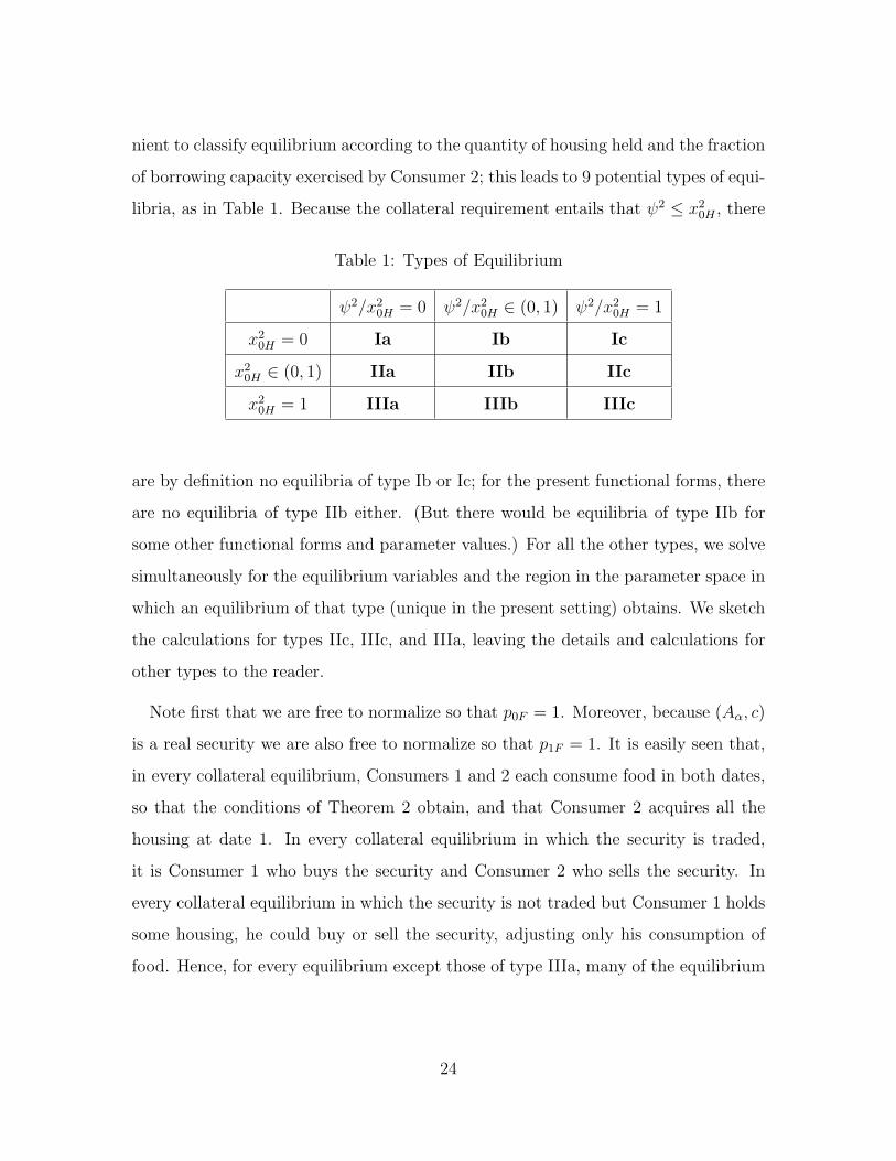
nient to classify equilibrium according to the quantity of housing held and the fraction

of borrowing capacity exercised by Consumer 2; this leads to 9 potential types of equi-

libria, as in Table 1. Because the collateral requirement entails that ψ2 ≤ x20H , there

Table 1: Types of Equilibrium

ψ2/x20H = 0 ψ2/x2

0H ∈ (0, 1) ψ2/x20H = 1

x20H = 0 Ia Ib Ic

x20H ∈ (0, 1) IIa IIb IIc

x20H = 1 IIIa IIIb IIIc

are by definition no equilibria of type Ib or Ic; for the present functional forms, there

are no equilibria of type IIb either. (But there would be equilibria of type IIb for

some other functional forms and parameter values.) For all the other types, we solve

simultaneously for the equilibrium variables and the region in the parameter space in

which an equilibrium of that type (unique in the present setting) obtains. We sketch

the calculations for types IIc, IIIc, and IIIa, leaving the details and calculations for

other types to the reader.

Note first that we are free to normalize so that p0F = 1. Moreover, because (Aα, c)

is a real security we are also free to normalize so that p1F = 1. It is easily seen that,

in every collateral equilibrium, Consumers 1 and 2 each consume food in both dates,

so that the conditions of Theorem 2 obtain, and that Consumer 2 acquires all the

housing at date 1. In every collateral equilibrium in which the security is traded,

it is Consumer 1 who buys the security and Consumer 2 who sells the security. In

every collateral equilibrium in which the security is not traded but Consumer 1 holds

some housing, he could buy or sell the security, adjusting only his consumption of

food. Hence, for every equilibrium except those of type IIIa, many of the equilibrium

24

variables can be determined quickly from first order conditions. In particular:

MU21H

p1H

=MU2

1F

p1F

(4)

MU10F

p0F

=MU1

(Aα,c)

qα(5)

It follows from (4) that p1H = 4. Because α ∈ [0, 4], the date 1 value of collateral

(weakly) exceeds the promise Aα, so Del(Aα, p) = α; hence MU1(Aα,c) = α. Now (5)

implies that qα = α. Summarizing: for all w ∈ (0, 18), all α ∈ [0, 4], and in every

equilibrium except those of type IIIa we have

p0F = 1 , p1F = 1 , p1H = 4 , qα = α , ψ1 = 0 , ϕ2 = 0 (6)

We begin by analyzing equilibrium of type IIc. Consumer 1 holds food and housing

at date 0, so he can trade housing for food or vice versa. Thus we have the first order

condition:

MU10F

p0F

=MU1

0H

p0H

(7)

Consumer 1 enjoys 1 util from living in the house at date 0 and 4 more utils by selling

the house at date 1 to buy 4 units of date 1 food. Hence MU10H = 5 and p0H = 5.

To solve for the remaining equilibrium variables we use Consumer 2’s date 0 first

order conditions – but the correct first order conditions may not be obvious. Because

Consumer 2 holds food and housing at date 0, it might appear by analogy with the

first order conditions for Consumer 1 that

MU20F

p0F

=MU2

0H

p0H

(8)

MU20F

p0F

=MU2

(Aα,c)

qα(9)

Consumer 2 enjoys 4 utils from living in the house at each date, so MU20H = 8. In

view of our earlier calculations, it follows from (8) that MU20F = 8/5 and from (9)

that MU20F = 1, which is nonsense.

25

The error in this analysis is that (8) and (9) are not the correct first order conditions

for Consumer 2. Consumer 2 can borrow against date 1 income by selling the security,

but selling the security requires holding collateral. By assumption, at equilibrium

x20H = ψ2, so Consumer 2 is exercising all of her borrowing power; hence she cannot

hold less housing without simultaneously divesting herself of some of the security and

cannot sell more of the security without simultaneously acquiring more housing.

The correct first order conditions for Consumer 2 take borrowing and collateral

constraints into account. On the one hand, buying an additional infinitesimal amount

ε of housing costs p0Hε, but of this cost αε can be borrowed by selling α units of

the security, using the additional housing as collateral, so the net payment is only

(p0H − α)ε. However, doing this will require repaying the loan in date 1, so the

additional utility obtained will not be 8ε but rather (8 − α)ε. On the other hand,

selling an additional ε units of food generates income of p0F ε at a utility cost of

MU20F ε. Hence the correct first order condition for Consumer 2 is not (8), but rather

1

x20F

=MU2

0F

p0F

=8− α

p0H − α=

8− α

5− α(10)

Consumer 2’s date 0 budget constraint is

(5− α)x20H + x2

0F = w (11)

Solving yields

x20F =

5− α

8− α, x2

0H =w − 5−α

8−α

5− α

From this we can solve for all the equilibrium consumptions and utilities

x1 =

(18− 5− α

8− α, 1−

w − 5−α8−α

5− α; 9 + α

[w − 5−α

8−α

5− α

]+ 4

[1−

w − 5−α8−α

5− α

], 0

)u1 = 32− w

x2 =

(5− α

8− α,w − 5−α

8−α

5− α; 9− α

[w − 5−α

8−α

5− α

]− 4

[1−

w − 5−α8−α

5− α

], 1

)

u2 = 8 + log(5− α)− log(8− α) +

(8− α

5− α

)w

26

(By definition, ψ2 = x20H and ϕ1 = ψ2.) Finally, the region in which equilibria are of

type IIc is defined by the requirement that x20H ∈ (0, 1), so

Region IIc =

{(w, α) :

5− α

8− α< w <

(5− α)(9− α)

8− α

}In equilibria of type IIIc, x2

0H = 1 and ψ2/x20H = 1 so Consumer 1 no longer holds

housing in date 0, and we cannot guess in advance what the price of housing will be

in period 0, but must solve for it along with the other variables. Reasoning as above,

we see that Consumer 2’s date 0 first-order condition and budget constraint are

8− α

p0H − α=

1

x20F

p0H − α+ x20F = w

Solving yields:

p0H = α+

(8− α

9− α

)w

x1 =

(18− w

9− α, 0; 9 + α, 0

)u1 = 27 + α− w

9− α

x2 =

(w

9− α, 1; 9− α, 1

)u2 = log

(w

9− α

)+ 17− α

The region in which equilibria are of type IIIc is determined by the requirements

that it be optimal for Consumer 2 to borrow the maximum amount possible, whence

x0F ≤ 1, and that Consumer 1 not wish to buy housing, whence p0H ≥ 5. Putting

these together yields:

Region IIIc =

{(w,α) :

(5− α

8− α

)(9− α) ≤ w ≤ (9− α)

}In region IIIa, the security is not traded but Consumer 2 holds all the housing and

some food at date 0, so Consumer 2 must be rich enough at date 0 to buy all the

27

housing without borrowing, and must be indifferent to trading date 0 food for date 0

housing or for the security. Her first order conditions and budget constraint at date

0 are:

MU2(A,c)

qα=

MU20F

p0F

(12)

MU20F

p0F

=MU2

0H

p0H

(13)

1 · x20F + p0H · 1 = w (14)

Solving yields

p0H =8w

9, x2

0F =w

9, qα =

αw

9

At these prices, Consumer 1 would like to sell the security, but is deterred from doing

so by the requirement to hold (expensive) collateral. Equilibrium consumptions and

utilities are:

x1 = (26− w, 0; 9, 0)

u1 = 35− w

x2 = (w

9, 1; 9, 1)

u2 = log(w

9

)+ 17

Finally, region IIIa is defined by the requirement that Consumer 2 be rich enough to

buy all the housing at date 0:

Region IIIa = {w : w ≥ 9}

Figure 1 depicts the various equilibrium regions and the price of housing in the

various regions; we summarize below, showing p0H , q (the prices that are not identical

across regions), consumptions and utilities in the non-empty regions. (We suppress

portfolio holdings.)

28

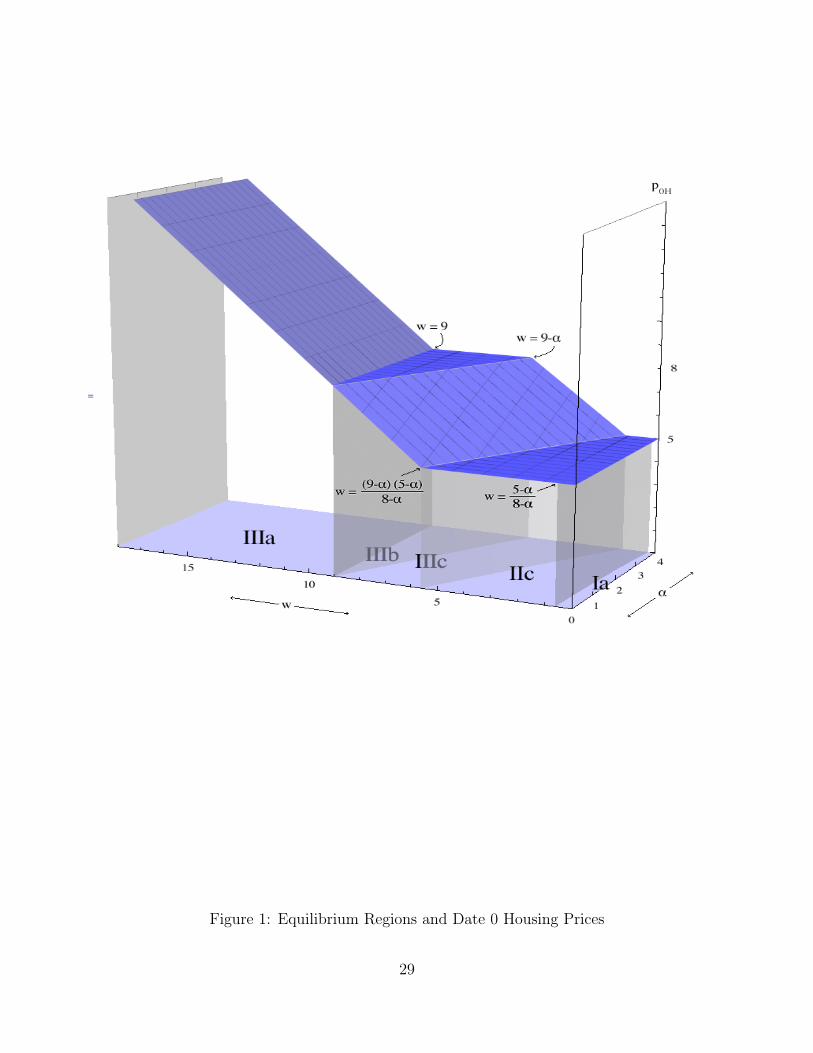
Figure 1: Equilibrium Regions and Date 0 Housing Prices

29

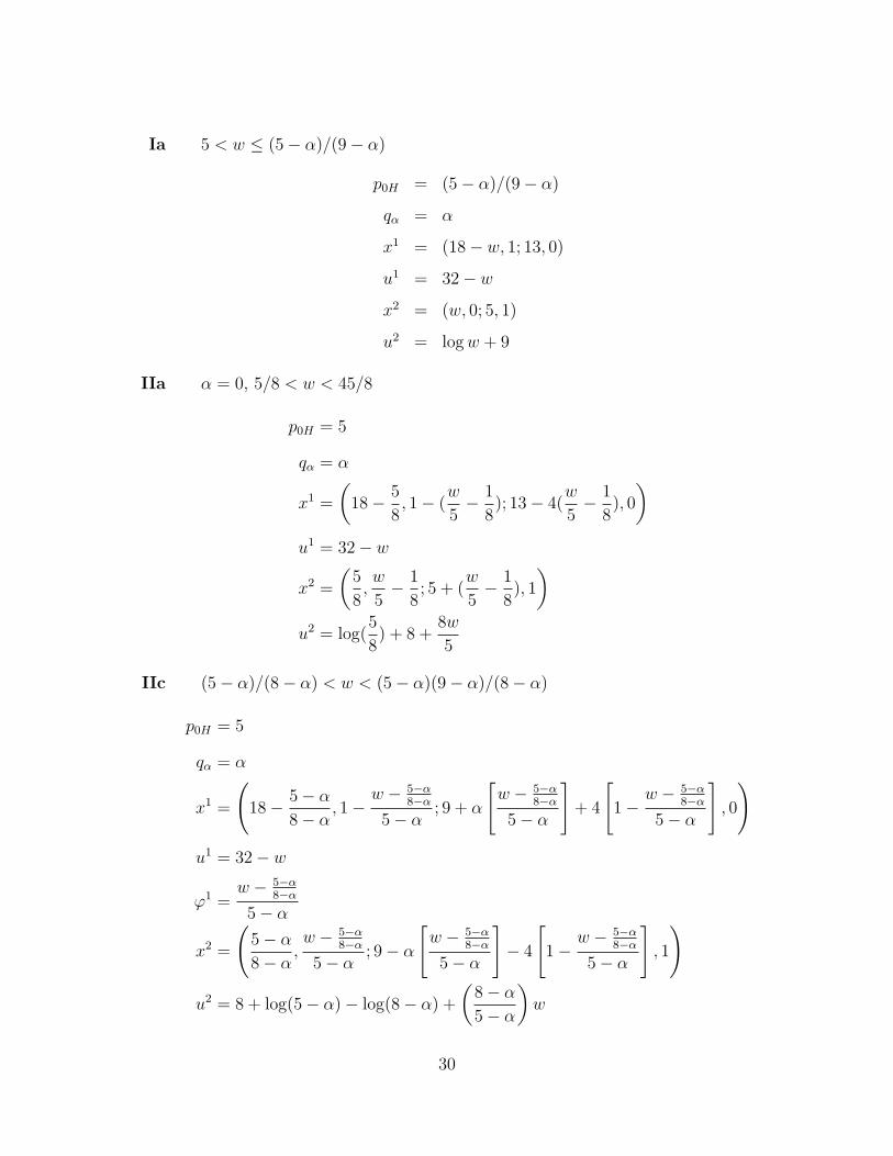
Ia 5 < w ≤ (5− α)/(9− α)

p0H = (5− α)/(9− α)

qα = α

x1 = (18− w, 1; 13, 0)

u1 = 32− w

x2 = (w, 0; 5, 1)

u2 = logw + 9

IIa α = 0, 5/8 < w < 45/8

p0H = 5

qα = α

x1 =

(18− 5

8, 1− (

w

5− 1

8); 13− 4(

w

5− 1

8), 0

)u1 = 32− w

x2 =

(5

8,w

5− 1

8; 5 + (

w

5− 1

8), 1

)u2 = log(

5

8) + 8 +

8w

5

IIc (5− α)/(8− α) < w < (5− α)(9− α)/(8− α)

p0H = 5

qα = α

x1 =

(18− 5− α

8− α, 1−

w − 5−α8−α

5− α; 9 + α

[w − 5−α

8−α

5− α

]+ 4

[1−

w − 5−α8−α

5− α

], 0

)u1 = 32− w

ϕ1 =w − 5−α

8−α

5− α

x2 =

(5− α

8− α,w − 5−α

8−α

5− α; 9− α

[w − 5−α

8−α

5− α

]− 4

[1−

w − 5−α8−α

5− α

], 1

)

u2 = 8 + log(5− α)− log(8− α) +

(8− α

5− α

)w

30

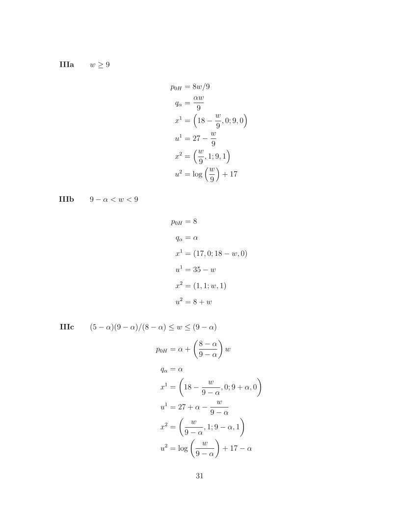
IIIa w ≥ 9

p0H = 8w/9

qα =αw

9

x1 =(18− w

9, 0; 9, 0

)u1 = 27− w

9

x2 =(w

9, 1; 9, 1

)u2 = log

(w9

)+ 17

IIIb 9− α < w < 9

p0H = 8

qα = α

x1 = (17, 0; 18− w, 0)

u1 = 35− w

x2 = (1, 1;w, 1)

u2 = 8 + w

IIIc (5− α)(9− α)/(8− α) ≤ w ≤ (9− α)

p0H = α+

(8− α

9− α

)w

qα = α

x1 =

(18− w

9− α, 0; 9 + α, 0

)u1 = 27 + α− w

9− α

x2 =

(w

9− α, 1; 9− α, 1

)u2 = log

(w

9− α

)+ 17− α

31

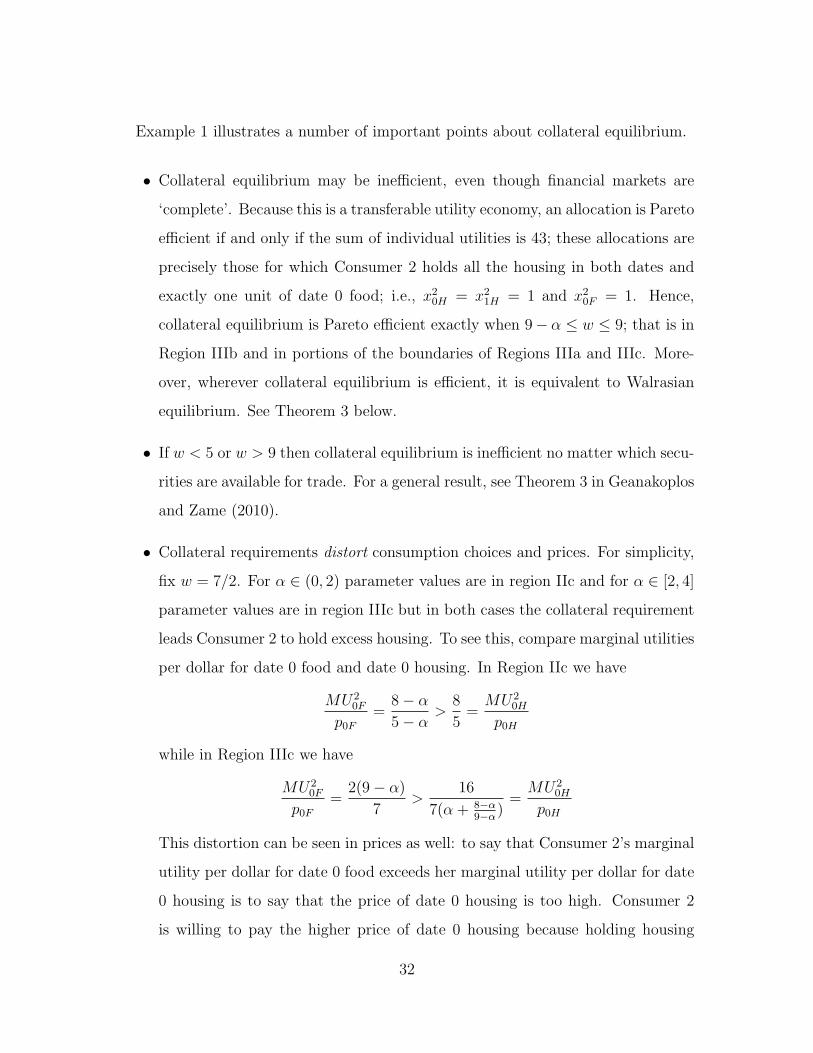
Example 1 illustrates a number of important points about collateral equilibrium.

• Collateral equilibrium may be inefficient, even though financial markets are

‘complete’. Because this is a transferable utility economy, an allocation is Pareto

efficient if and only if the sum of individual utilities is 43; these allocations are

precisely those for which Consumer 2 holds all the housing in both dates and

exactly one unit of date 0 food; i.e., x20H = x2

1H = 1 and x20F = 1. Hence,

collateral equilibrium is Pareto efficient exactly when 9− α ≤ w ≤ 9; that is in

Region IIIb and in portions of the boundaries of Regions IIIa and IIIc. More-

over, wherever collateral equilibrium is efficient, it is equivalent to Walrasian

equilibrium. See Theorem 3 below.

• If w < 5 or w > 9 then collateral equilibrium is inefficient no matter which secu-

rities are available for trade. For a general result, see Theorem 3 in Geanakoplos

and Zame (2010).

• Collateral requirements distort consumption choices and prices. For simplicity,

fix w = 7/2. For α ∈ (0, 2) parameter values are in region IIc and for α ∈ [2, 4]

parameter values are in region IIIc but in both cases the collateral requirement

leads Consumer 2 to hold excess housing. To see this, compare marginal utilities

per dollar for date 0 food and date 0 housing. In Region IIc we have

MU20F

p0F

=8− α

5− α>

8

5=MU2

0H

p0H

while in Region IIIc we have

MU20F

p0F

=2(9− α)

7>

16

7(α+ 8−α9−α

)=MU2

0H

p0H

This distortion can be seen in prices as well: to say that Consumer 2’s marginal

utility per dollar for date 0 food exceeds her marginal utility per dollar for date

0 housing is to say that the price of date 0 housing is too high. Consumer 2

is willing to pay the higher price of date 0 housing because holding housing

32

enables her to borrow; that is, she derives a collateral value from housing as

well as a consumption value. Similarly, Consumer 2 finds the marginal utility

per dollar for date 0 food to be higher than the marginal utility of making the

payments on the security; the price of the security is “too high” as well – she

experiences a liquidity wedge.

• As we have shown in Theorem 2 above, in every region where CE 6= GEI, some

consumer experiences a collateral value and liquidity wedge. In Regions IIc

and IIIc this is Consumer 2. In the portion of Region IIIa where w > 9, it is

Consumer 1 who experiences collateral values and a liquidity wedge, although

Consumer 1 neither holds housing nor sells the security.

• The effects of collateral requirements on welfare are subtle. Again, fix w = 7/2.

Increases in α (equivalently, decreases in the down payment requirement) make

it possible for consumers of type 2 to access more date 1 wealth. For α ∈ [0, 2),

this makes it possible for consumers of type 2 to afford more housing; the net

result is Pareto improving. For α ∈ [2, 4], however, consumers of type 2 already

own all the available houses, so increasing α only leads to more competition

among them, which serves only to drive up the price of date 0 housing (from

p0H = 5 when α = 2 to p0H = 34/5 when α = 4). This price increase makes

Consumers of type 1 better off but makes Consumers of type 2 worse off.

6 Efficiency

We close the circle of ideas around distortion by showing that, modulo technical

assumptions, efficient collateral equilibria are Walrasian.

Theorem 3 (Efficient Collateral Equilibria are Walrasian) Let E = 〈(ei, ui),A〉

be an economy with collateralized securities and let 〈p, q, xi, ϕi, ψi〉 be an equilibrium

33

for E. Assume as in Theorem 2 that each consumer’s equilibrium consumption is non-

zero in each spot, that each consumer’s consumption of goods not used as collateral is

non-zero at date 0, that utilities are differentiable at equilibrium consumptions, and

that at least one consumer’s consumption of every good is strictly positive. If the col-

lateral equilibrium allocation (xi) is a Pareto optimal allocation and we define prices

π by πs` = MUhs`/µ

h0 , then 〈π, xi〉 is a Walrasian equilibrium for the economy 〈ei, ui〉.

Proof There is no loss in assuming that all the contracts (Aj, cj) are traded in the

equilibrium; otherwise we can simply delete non-traded contracts without disturbing

the equilibrium.

Assume that consumer h’s consumption of every good is strictly positive. If agent

i is buying the contract (Aj, cj) then qj = FV ij (otherwise i should have bought

more or less of this contract). Whether or not consumer h had been a buyer of this

contract, we must have qj = FV hj , for otherwise h could buy a little of (Aj, cj) or sell

a little to one of the buyers i of (Aj, cj) (keeping in mind that there must be buyers,

since every contract is traded), making or receiving payment of value qj in date 0

goods that i is consuming at date 0, and delivering in each state s a tiny bit more in

value than Del((Aj, cj), s, p) in goods i is consuming in equilibrium. (This is feasible

because h is consuming strictly positive amounts of all goods, and so can make the

deliveries by reducing his consumption.) This would make both h and i better off,

which would contradict Pareto efficiency. As in the proof of Theorem 2 it follows that

for all goods k, p0k = FV h0k ≡ π0k. And of course from the fact that h is optimizing

in the collateral equilibrium and chose positive consumption of each good, it must be

that ps is proportional to πs for all s ≥ 1.

To see that 〈π, x〉 must be a Walrasian equilibrium, choose aj ∈ RL(1+S) so that

qj = −p0 · aj0 and Del((Aj, cj), s, p) = ps · aj

s for all s ≥ 1. Because qj = FV hj , it

follows that π · aj = 0, and hence that for each agent i, xi ∈ BW (ei, π). Since (xi) is

a Pareto efficient allocation, 〈π, x〉 must be a Walrasian equilibrium.

34

7 Default, Crashes and Welfare

This Section makes a number of related points. The first point is that default —

although suggestive of inefficiency — may be welfare enhancing.14 More precisely, as

Example 2 shows, levels of collateral that are socially optimal may lead to default

with positive probability. The second point is that there is a link between collateral

requirements and future prices. Lower collateral requirements lead buyers to take

on more debt; the difficulties of servicing this debt can lead to reduced demand and

lower prices — even to crashes — in the future. Importantly, such a crash occurs

precisely because lower collateral requirements encourage borrowers to take on more

debt than they can service. As Example 2 also shows, despite such crashes, lower

collateral requirements may be welfare enhancing. The third point is that although

the set of securities available for trade is given exogenously as part of the data of

the model, the set of securities that are actually traded is determined endogenously

at equilibrium. Thus, we may view the financial structure of the economy as chosen

by the competitive market. As Example 3 shows, the market may choose levels

of collateral that lead to default with positive probability, and this choice may be

efficient; even if all possible securities are available for trade, the market may choose

an incomplete set to actually be traded at equilibrium. Theorem 4 identifies a context

in which the market choice of securities (in particular collateral levels) is necessarily

efficient.

Example 2 (Default and Crashes) We construct a variant on Example 1. Rather

than present a full-blown analysis in the style of Example 1, we fix endowments and

take only the security promise as a parameter, which makes it easier to focus on the

points of interest.

There are two states of nature and two goods: Food, which is perishable, and

14A similar point has been made, in different contexts, by Zame (1993), Sabarwal (2003) and

Dubey, Geanakoplos, and Shubik (2005).

35

Housing, which is durable. There are two (types of) consumers, with endowments

and utility functions:

e1 = (29/2, 1; 9, 0; 9, 0)

u1 = x0F + x0H + (1/2)(x1F + x1H) + (1/2)(x2F + 3x2H)

e2 = (7/2, 0; 9, 0; 5/2, 0)

u2 = log x0F + 4x0H + (1/2)(x1F + 4x1H) + (1/2)(x2F + 4x2H)

Consumer 1 has constant marginal utility of consumption for food and housing at each

date/state; Consumer 2 has constant marginal utility for housing at each date/state

but decreasing marginal utility for date 0 food; both consumers view the states as

equally likely. Note the only differences from Example 1 are that Consumer 1 likes

housing better in state 2 and Consumer 2 is poor in state 2 – the ’bad’ state.

Suppose that a single security – a mortgage – Aα = (αp1F , αp2F ; δ0H), promising

the value of α units of food and collateralized by 1 unit of housing, is available for

trade; we take α ∈ [0, 4] as a parameter.15 (Equivalently, we could consider securities

that promise to deliver the value of one unit of food and are collateralized by 1/α

units of housing.) We distinguish four regions; in each there is a unique equilibrium.

In Region I, α is sufficiently small that Consumer 2 cannot borrow enough to buy all

the housing at date 0, but buys the remaining housing in date 1. In Region II, α is

large enough that Consumer 2 can buy all the housing at date 0 but small enough

that she will be able to honor her promises in both states at date 1 and retain all the

housing at date 1. In Region III, Consumer 2 will honor her promises but will not

be able to retain all the housing. In Region IV, Consumer 2 will default. Finally, at

the boundary of Regions II and III, equilibrium consumptions are determinate but

prices are indeterminate. The calculations in Regions I, II are almost identical to

those in Example 1; the calculations for Regions III, IV follow the same method with

the appropriate changes to incorporate default.

15As before, the case α > 4 reduces to the case α = 4.

36

• Region I: α ∈ [0,2)

Consumers 1 and 2 both hold date 0 housing; Consumer 2 borrows as much as

she can in date 0 and honors her promises in both states at date 1.

p = (1, 5; 1, 4; 1, 4)

qα = α

x1 =

(18− 5− α

8− α, 1− 7

2(5− α)+

1

8− α; 9 + α, 0; 9 + α, 0

)x2 =

(5− α

8− α,

7

2(5− α)− 1

8− α; 9− α, 1;

5

2− α, 1

)• Region II: α ∈ [2,5/2)

Consumer 2 holds all the housing at both dates; Consumer 2 borrows as much

as she can in date 0 and honors her promises in both states at date 1.

p =

(1, α+

(8− α

9− α

)(7

2

); 1, 4; 1, 4

)qα = α

x1 =

(18− 7

2(9− α), 0; 9 + α, 0; 9 + α, 0

)x2 =

(7

2(9− α), 1; 9− α, 1;

5

2− α, 1

)• Boundary between Regions II, III: α = 5/2

Consumer 2 holds all the housing at both dates; Consumer 2 borrows as much

as she can in date 0; Consumer 2 honors her promises in both states at date

1. In the bad state, Consumer 2 holds all the housing and no food so p2H is

37

indeterminate.

p =

(1,

5

2+

(7

2

)(11

13

); 1, 4; 1, p2H

)p2H ∈ [3, 4]

qα = α

x1 =

(18− 7

13, 0;

23

2, 0;

23

2, 0

)x2 =

(7

13, 1;

13

2, 1; 0, 1

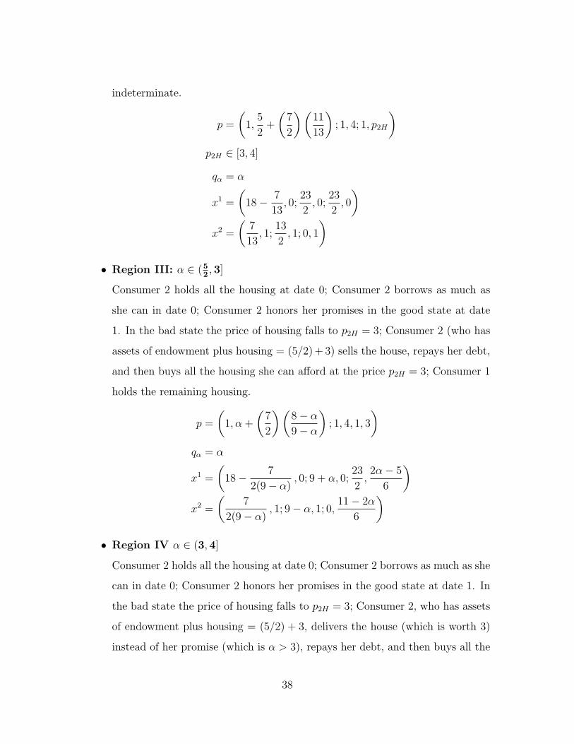
)• Region III: α ∈ (5

2,3]

Consumer 2 holds all the housing at date 0; Consumer 2 borrows as much as

she can in date 0; Consumer 2 honors her promises in the good state at date

1. In the bad state the price of housing falls to p2H = 3; Consumer 2 (who has

assets of endowment plus housing = (5/2) +3) sells the house, repays her debt,

and then buys all the housing she can afford at the price p2H = 3; Consumer 1

holds the remaining housing.

p =

(1, α+

(7

2

)(8− α

9− α

); 1, 4, 1, 3

)qα = α

x1 =

(18− 7

2(9− α), 0; 9 + α, 0;

23

2,2α− 5

6

)x2 =

(7

2(9− α), 1; 9− α, 1; 0,

11− 2α

6

)• Region IV α ∈ (3,4]

Consumer 2 holds all the housing at date 0; Consumer 2 borrows as much as she

can in date 0; Consumer 2 honors her promises in the good state at date 1. In

the bad state the price of housing falls to p2H = 3; Consumer 2, who has assets

of endowment plus housing = (5/2) + 3, delivers the house (which is worth 3)

instead of her promise (which is α > 3), repays her debt, and then buys all the

38

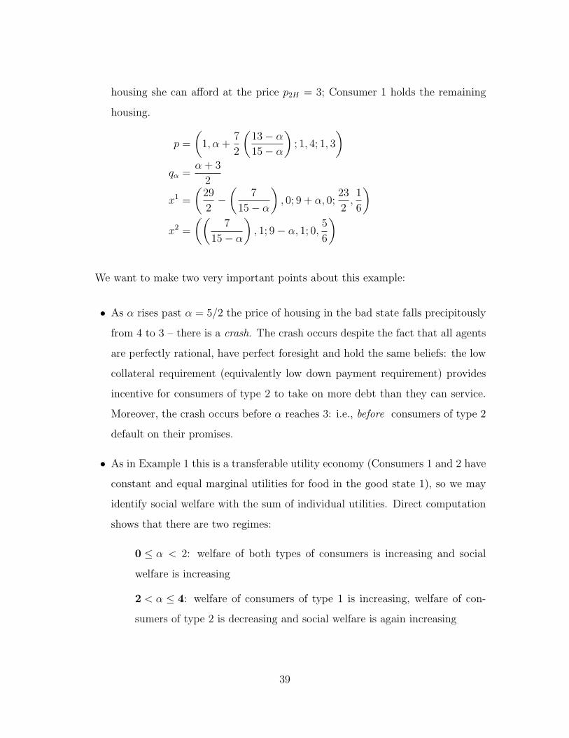
housing she can afford at the price p2H = 3; Consumer 1 holds the remaining

housing.

p =

(1, α+

7

2

(13− α

15− α

); 1, 4; 1, 3

)qα =

α+ 3

2

x1 =

(29

2−(

7

15− α

), 0; 9 + α, 0;

23

2,1

6

)x2 =

((7

15− α

), 1; 9− α, 1; 0,

5

6

)

We want to make two very important points about this example:

• As α rises past α = 5/2 the price of housing in the bad state falls precipitously

from 4 to 3 – there is a crash. The crash occurs despite the fact that all agents

are perfectly rational, have perfect foresight and hold the same beliefs: the low

collateral requirement (equivalently low down payment requirement) provides

incentive for consumers of type 2 to take on more debt than they can service.

Moreover, the crash occurs before α reaches 3: i.e., before consumers of type 2

default on their promises.

• As in Example 1 this is a transferable utility economy (Consumers 1 and 2 have

constant and equal marginal utilities for food in the good state 1), so we may

identify social welfare with the sum of individual utilities. Direct computation

shows that there are two regimes:

0 ≤ α < 2: welfare of both types of consumers is increasing and social

welfare is increasing

2 < α ≤ 4: welfare of consumers of type 1 is increasing, welfare of con-

sumers of type 2 is decreasing and social welfare is again increasing

39

In particular, social welfare attains its maximum when α = 4, so collateral

levels that lead to a crash (and to default) – with probability 1/2 – are socially

efficient.

When α > 3, it seems natural to think of the security Aα as a sub-prime mortgage,

so we might draw the moral that subprime mortgages can improve social welfare.

In our framework, the set of securities available for trade is given exogenously, but

the set actually traded is determined endogenously at equilibrium. Because the former

set might be very large (conceptually, all conceivable securities might be offered) we

can view the security market structure itself as determined by the action of the

competitive market. As we see below, the result can be an endogenously incomplete

security market (even when a complete set of securities is available for trade) and to

default at equilibrium (even when securities that do not lead to default are available

for trade).

Example 3 (Which Securities are Traded?) We maintain the entire structure

of Example 2, except that some set {(Aj, cj)} of securities is available for trade. To

be consistent with our framework, we assume the set of available securities is finite,

but, at least conceptually, we might imagine that all possible collateral requirements

are offered. Because only housing is durable, we assume that only housing is used as

collateral; there is no loss in normalizing so that cj = δ0H for each j.

In this setting, only Consumer 2 will sell securities (borrow); we assert that Con-

sumer 2 will sell only that security which offers her the largest liquidity wedge. (If

more than one security offers Consumer 2 the largest liquidity wedge, Consumer 2

might sell any or all of them.) To see this, suppose that at equilibrium Consumer 2

sells (Aj, cj) but that LW 2(Ak,ck)

> LW 2(Aj ,cj). Because both securities require the same

collateral Consumer 2 could sell ε fewer shares of (Aj, cj) and ε more shares of (Ak, ck)

without violating her collateral constraint. The definition of liquidity wedge means

40

that this change would strictly improve Consumer 2’s utility, which would contradict

the requirement that Consumer 2 optimizes at equilibrium.

Because liquidity wedges depend on the equilibrium prices and consumptions, it is

not in general possible to order a priori the liquidity wedges of given securities and

hence to know which securities will be traded and which will not be. Instead, we

analyze two particularly interesting scenarios.

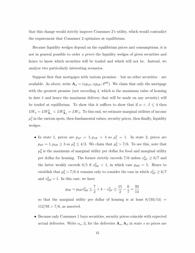
Suppose first that mortgages with various promises – but no other securities – are

available. As above, write Aα = (αp1F , αp2F ; δ0H). We claim that only the mortgage

with the greatest promise (not exceeding 4, which is the maximum value of housing

in date 1 and hence the maximum delivery that will be made on any security) will

be traded at equilibrium. To show this it suffices to show that if α < β ≤ 4 then

LWα = LW 2Aα

< LW 2Aβ

= LWβ. To this end, we estimate marginal utilities of income

µ2s in the various spots, then fundamental values, security prices, then finally, liquidity

wedges.

• In state 1, prices are p1F = 1, p1H = 4 so µ21 = 1. In state 2, prices are

p2F = 1, p2H ≥ 3 so µ22 ≤ 4/3. We claim that µ2

0 > 7/6. To see this, note that

µ20 is the maximum of marginal utility per dollar for food and marginal utility

per dollar for housing. The former strictly exceeds 7/6 unless x20F ≥ 6/7 and

the latter weakly exceeds 8/5 if x20H < 1, in which case p0H = 5. Hence to

establish that µ20 > 7/6 it remains only to consider the case in which x2

0F ≥ 6/7

and x20H = 1. In this case, we have

p0H = p0Hx20H ≤ 7

2+ 4− x2

0F ≤15

2− 6

7=

93

14

so that the marginal utility per dollar of housing is at least 8/(93/14) =

112/93 > 7/6, as asserted.

• Because only Consumer 1 buys securities, security prices coincide with expected

actual deliveries. Write αs, βs for the deliveries Aα,Aβ in state s so prices are

41

qα = (1/2)(α1 + α2) and qβ = (1/2)(β1 + β2).

• The definitions, the above estimates and some algebra yield(1

2

)LWβ − LWα = [qβ −

(1

2

)(µ2

1β1 + µ22β2)]− [qα −

(1

2

)(µ2

1α1 + µ22α2)]

=

(1

2

){[(β1 + β2)− (β1 + µ2

2β2)]− [(α1 + α2)− (α1 + µ22α2)]

}=

(1

2

)[(µ2

0 − 1)(β1 − α1) + (µ20 − µ2

2)(β2 − α2)]

>

(1

12

)[(β1 − α1)− (β2 − α2)

]Because the delivery on any security will be the minimum of its promise and

the value of collateral if follows that α1 = α, β1 = β and β − α ≥ (β2 − α2).

Hence LWβ − LWα > 0, as asserted.

In particular, if A4 – the mortgage with the largest promise – is offered, then only

this mortgage will be traded, even though (as shown above), this leads to default in

equilibrium.

Now suppose that all possible securities are offered. We assert that in equilibrium

only those securities (with collateral δ0H) whose deliveries are 4 in state 1 and 3 in

state 2 will actually be traded, and that equilibrium commodity prices and consump-

tions coincide with the equilibrium when only the security A4 above is traded. To see

this fix an equilibrium. First suppose the security B is traded and that Del1B < 4.

Let B′ be any security with the same collateral and state 2 promise (hence delivery) as

B, but which promises (hence delivers) 4 units of account in state 1. Arguing exactly

as above, we see that B′ offers Consumer 2 (the only seller of B) a strictly greater

liquidity wedge than does B. Hence Consumer 2 would strictly prefer to sell B′ rather

than B, which is a contradiction. We conclude that if B is traded then Del1B = 4.

Now suppose two securities B1,B2 are traded, that Del1B1 = Del1B

2 = 4 and that

β1 = Del2B1 < Del2B

2 = β2. Arguing as before, we see that Consumer 2’s date 0

42

first-order conditions require:

8− 12(4 + β1)

p0H − 12(4 + β1)

=1

x0F

=8− 1

2(4 + β2)

p0H − 12(4 + β2)

This entails β1 = β2 which is a contradiction, so we conclude that all securities traded

at equilibrium have the same deliveries: 4 in state 1 and β ≤ 4 in state 2. If β > 3

we can argue exactly as in Example 2 to show that default will occur in state 2 and

hence p2H = 3, whence delivery will be only 3, a contradiction. If β < 3 arguing as

before shows that at equilibrium p2H = 4 whence any security whose delivery is 4 in

state 1 and β′ in state 2, with β < β′ < 3, will offer Consumer 2 a greater liquidity

wedge. This is again a contradiction, so we conclude that only those securities (with

collateral δ0H) whose deliveries are 4 in state 1 and 3 in state 2 will actually be traded.

It follows immediately that equilibrium commodity prices and consumptions coincide

with the equilibrium when only the security A4 (see Example 2) is traded.

Note that even though all possible securities are available, the set of securities

that are traded at equilibrium is endogenously incomplete. Note in particular that

Arrow securities are not traded, even though they are available, because they make

extremely inefficient use of the available collateral.

In the two scenarios analyzed in Example 3, the market chooses socially efficient

promises – even though those promises may lead to default. Characterizing situations

when the market does or does not choose socially efficient sets of securities – or at least

Pareto undominated sets of securities – seems an important and difficult question, to

which we do not know the answer. (Indeed, because multiple equilibria are possible,

it is not entirely clear precisely how to formulate the question.) However, we can give

an unambiguous answer about Pareto domination in at least one important case: if

date 1 prices do not depend on the choices of securities.

Theorem 4 (Constrained Optimality) Every set of collateral equilibrium plans

is Pareto undominated among all sets of plans that:

43

(a) are socially feasible;

(b) given whatever date 0 decisions are assigned, respect each consumer’s budget set

at every state s at date 1 at the given equilibrium prices;

(c) call for deliveries on securities that are the minimum of the promise and the

value of collateral.

Proof of Theorem 4 Let 〈p, q, (xi, ϕi, ψi)〉 be an equilibrium, and suppose that

(xi, ϕi, ψi) is a family of plans meeting the given conditions that Pareto dominates

the equilibrium set of plans. By assumption, all the alternative plans are feasible,

meet the budget constraints at each state at date 1, and call for deliveries that are

the minumum of promises and the value of collateral, Optimality of the equilibrium

plans at prices p, q means, therefore, that all the alternative plans (xi, ϕi, ψi) fail the

budget constraints at date 0. Because the alternative set of plans is socially feasible,

summing over consumers yields a contradiction.

In particular, prohibiting trade in certain securities – for example, those that are

leveraged above some threshold – cannot lead to a Pareto improvement unless date

1 prices change; if date 1 prices do not change, the market chooses the security

structure efficiently. In an environment or model in which only one good is available

for consumption at date 1, collateral equilibrium is always constrained efficient and

the market chooses the security structure efficiently; compare Kilenthong (2006).

8 Some Comparative Statics

Examples 1, 2, 3 illustrate some important comparative statics conclusions but only

in particular settings with particular parameters. It seems desirable to identify other

settings in which comparative statics conclusions can be reached. However, it is noto-

riously difficult to derive robust comparative statics theorems in general equilibrium

44

theory; it becomes harder when markets are incomplete and harder still when col-

lateral is involved. Here we introduce a particular class of models in which some

comparative statics conclusions are possible. The models we use assume quasi-linear

utility functions (in each state); this eliminates income effects and all the relative

price changes that might occur as the natural result of income effects, allowing more

precise predictions. The absence of income effects also allows us to isolate changes

that occur even in the absence of income effects and the attendant price changes.

Of course one must bear in mind that sometimes these price changes are the most

interesting aspects of the comparative statics, and they will be absent in our models.

We consider economies in which utility functions are separable across time/states/goods

and quasi-linear in a “money” good. It is convenient to number so that there are 1+L

goods 0, 1, . . . , L available in each spot and usem to denote good 0, the money good; a

typical consumption vector is (m,x) = (m0, x0;m1, x1, . . . ,ms, xs). We assume utility

functions enjoy the following properties:

• Utility functions are separable across time/states/goods and quasi-linear in the

money good:

ui(m,x) = m0 +L∑

`=1

ui0`(x0`) + δi

S∑s=1

γis

[ms +

L∑`=1

uis`(xs`)

]

Here, (γis) is a probability distribution on states of nature and δi is a discount

factor (which will serve us as a proxy for liquidity).

• For each s, ` 6= 0 the function uis` is smooth, has strictly positive first derivative

and strictly negative second derivative, and satisfies the Inada condition

limxs`→0

duis`

dxs`

= ∞

We assume that each security is collateralized by a single good (and there is no loss

in assuming that each collateral requirement is a single unit of the relevant good) and

that security promises in each state depend only on prices in that state. We focus

45

attention entirely on interior equilibria in which every agent consumes a positive

amount of each good in each spot, and we assume that the price of the money good

is equal to 1 in every spot.16

With these assumptions, interior equilibria of these economies can be characterized

very simply. For each state s 6= 0 and as ∈ RL++, define

Ws(as) = Ws(as1, ..., asL) = max{xi

s:P

i xis≤as}

∑i

uis(x

is)

Given our assumptions, Ws is smooth. Moreover, for all k, i we have:

∂W (a)

∂ask

=∂ui

s(xis)

∂xsk

for every agent i, where the xis are the allocations that solve the maximization defining

Ws. For s ≥ 1, set as =∑

h[ehs + Fs(e

h0)] and define commodity prices to be psk =

∂Ws(as)∂ask

for all k and consumptions to be the corresponding solutions xis. For each

security (Aj, cj), we can then deduce the equilibrium delivery, and for each agent i

and commodity k we can define the durable value of k

Dsj = Del((Aj, cj), s, p) = min(Asj(ps), ps · Fs(cj))

dik = δi

∑s

γisps · Fs(δ0k)

We can also deduce the price of each security as the maximum that anybody would

pay to buy it:

qj = maxh

δh∑

s

γhsDsj

This in turn allows us to define the liquidity wedge of any security j to any agent i

LW ij = qj − δi

∑s

γisDsj

16The Inada conditions guarantee that equilibrium consumption of non-money goods will be

strictly positive in each state. Instead of assuming that consumption of the money good is strictly

positive in each spot, we could assume that the money good could be consumed in either positive

or negative amounts.

46

By Theorem 2, the collateral value of k to any agent i must be the maximum liquidity

wedge over contracts using k as collateral

CV ik = max

{j:cjk=1}[qj − δi

∑s

γisDsj]

This in turn permits us to compute the collateral plus future value of any good k to

any agent i

V ik = CV i

k + dik = max

{j:cjk=1}[qj − δi

∑s

γisDsj] + δi

∑s

γisps · Fs(δ0k)

Finally, for any a0 ∈ RL++, define

W0(a0) = W0(a01, ..., a0L) = max{xi

0:P

i xi0≤a0}

∑i

[ui0(x

i0) + V i · xi

0]

Given our assumptions, W0 is differentiable and

∂W0(a)

∂a0`

=∂ui

0(xi0)

∂x0`

+ V i`

for every agent i and commodity `, where the xi0 are the allocations that solve the

maximization defining W. For s ≥ 1, take a0 =∑

h eh0 and take equilibrium price

p0k = ∂W0(a)∂a0k

for all k and take the equilibrium consumptions to be the corresponding

solutions xi0.

This still leaves the security trades and m allocations to specify. Every holder i of a

durable good k with a positive collateral value to him will sell a corresponding number

of securities with the maximal liquidity wedge. The purchases of these securities

can be divided arbitrarily among the agents who are indifferent to buying them.

Afterward the mis can be uniquely assigned so that every agent balances his budget

in every state. When initial endowments eism of the m good are sufficiently high, this

leaves us with an allocation of positive values for the mis.

Lemma If endowments eism are sufficiently large then there is a unique collateral

equilibrium; consumptions, commodity prices and security prices are defined by the

equations above.

47

8.1 Collateral Value, Leverage and Asset Prices

Geanakoplos (2003) argues by example that, as leverage increases, security prices

rise. An important part of the argument is an income effect: When cash constrained

buyers are given access to more loans, they can spend more money on assets, driving

up their prices. Even if the buyers had positive consumption, and were thus choosing

not to spend more on assets in the original equilibrium, the loans would allow them

to increase consumption. Assuming diminishing marginal utility, the increased con-

sumption increases the fundamental value of the assets to them, and so they would

spend part of the loan on the assets and increase their prices. This logic is illustrated

by Example 1 in Section 5.

In the current context, this income effect logic is completely absent (in interior

equilibria). However, as noted in Fostel-Geanakoplos (2008), there is still a connection

between raising (lowering) collateral requirements and decreasing (increasing) asset

prices that operates through the collateral value.

Theorem 5 (Leverage and Security Pricing) Fix the unique interior collateral

equilibrium with commodity prices p for an economy satisfying the assumptions above.

If leverage on some commodity ` is reduced by replacing some securities (Aj, cj)

which use commodity 0` as collateral by securities (A′j, c

′j) with the same collateral

but smaller promises, then in the interior equilibrium for the new economy, the price

of the commodity 0` does not rise: p′0` ≤ p0`. If, in the original economy the commod-

ity 0` had positive collateral value to some agent i∗, and deliveries are strictly reduced

for all securities using 0` as collateral, then the price of the commodity 0` strictly

falls: p′0` < p0`.

Proof Note that in the new economy q′j = 1(1+εj)

qj and for all i, LV ′ij = 1

(1+εj)LV i

j .

Hence V ′i` ≤ V i

` for all i. Some agent i must be consuming at least as much of ` at

48

state 0 in the new economy as in the old, hence by diminishing marginal utility of `

p′` =dui

0`(x′i0 )

dxi0`

+ V ′i` ≤ dui

0`(xi0)

dxi0`

+ V i` = p`

If all leverage on ` is similarly reduced, then we deduce in addition that CV ′i∗` < CV i∗

`

and thus V ′i∗` < V i∗

` . If i∗ consumes at least as much of ` in state 0 in the new economy,

then we deduce from the above equation with i∗ = i that p′` < p`. If i∗ consumes

strictly less of ` in state 0 in the new equilibrium then there is some other agent i

who consumes stricty more; then because ui0` displays strictly diminishing marginal

utility and V ′i` ≤ V i

` , the result follows.

8.2 Flight to Collateral

Fostel and Geanakoplos (2008) argue by example that, as liquidity conditions de-

teriorated, goods/assets which could serve as collateral will fall less in value than

goods/assets which could not serve as collateral – so there would be a “flight to col-

lateral”. This argument provides an explanation of why treasury bonds did not lose

as much value as corporate bonds in the crisis of 2008 that stands in contrast to the

usual “flight to quality” explanation based on shifts in risk aversion. We can illustrate

flight to collateral in the present class of economies.

The good m in our TU economy is the catch-all for other uses of liquidity. As m0

becomes more valuable to an agent relative to future ms, he becomes more anxious

to get his hands on money now; he can be said to be more liquidity needy. The

next theorem shows that when this happens, all goods with durable value go strictly

down in value except those goods that are perfect collateral, i.e. which can be used

to promise their full future value.

Theorem 6 (Flight to Collateral) Fix the interior collateral equilibrium for an

economy satisfying the assumptions above. Suppose that in the equilibrium some agent

i∗ is not the unique buyer of any security. Consider a new economy identical to the

49

old except that i∗ becomes more liquidity constrained, in the sense that δ′i∗< δi∗.

Consider any good 0`′ and suppose i∗ is selling at least one security which uses 0`′ as

collateral

• If `′ is not a perfect collateral (that is, for all securities j that i∗ sells and that

use `′ as collateral there is at least one state s in which that Asj(ps) < ps·Fs(cj)),

then the price of 0`′ is strictly lower in the new economy: p′0`′ < p′0`′.

• If `′ is a perfect collateral (that is, for all securities j that i∗ sells and that use

`′ we have Asj(ps) ≥ ps · Fs(cj)), then the price of 0` will be the same in the

new economy: p′0`′ < p′0`′.

Proof Note first that since i∗ is not the unique buyer of any security in the old

equilibrium, the new security prices of traded securities are exactly the same as the

old security prices (though untraded securities, for which i∗ may have had the uniquely

highest valuation, may have gone down in value). Furthermore, the durable value of

`′ falls for i∗, because in some state it has positive value and is now discounted more,

and though the collateral value of `′ for i∗ might also rise, it cannot rise enough

to offset it, so V ′i∗`′ < V i∗

`′ . Hence by the argument in the proof of Proposition 1,

p′0`′ < p0`′ . On the other hand, the collateral value of ` to i∗ does rise just enough to

offset its fall in durable value to i∗, so V ′i` = V i

` for all i. Hence p′0` = p0`.

8.3 Liquidity, Leverage, and Asset Pricing

We shall now show that when an agent requires more liquidity needs he will seek

higher leverage. Define the loan-to-value an agent i uses in purchasing a commodity

0k as

LTV i0k =

∑{j:cj

0k>0} ψijqj

p0kxi0k

50

Theorem 7 (Liquidity and Leverage) Assume the hypotheses of Theorem 6 and

that 0`′ gives i∗ strictly positive collateral value in the old equilibrium. Then the loan-

to-value that i∗ uses to buy 0`′ will be strictly higher in the new equilibrium than in

the old equilibrium.

Proof First we shall show that if agent i∗ uses `′ as collateral to back a loan j′ in

the new equilibrium and used `′ as collateral to back a loan j in the old equilibrium,

then q′j′ ≥ qj. From Proposition 2 we already know that q′j′ = qj′ and q′j = qj, hence

LW ′i∗j′ = q′j′ − δ′i

∗∑s

γi∗

s D′sj′ = qj′ − δ′i

∗∑s

γi∗

s Dsj′

LW ′i∗j = q′j − δ′i

∗∑s

γi∗

s Dsj = qj − δ′i∗∑

s

γi∗

s Dsj

LW i∗

j′ = qj′ − δi∗∑

s

γi∗

s Dsj′

LW i∗

j = qj − δi∗∑

s

γi∗

s Dsj

From the same hypothesis on which loans i∗ used `′ to back, we must have LW ′i∗j′ ≥

LW ′i∗j and LW i∗

j ≥ LW i∗

j′ , which implies that

LW ′i∗j′ − LW i∗

j′ ≥ LW ′i∗j − LW i∗

j

(δi∗ − δ′i∗)∑

s

γi∗

s Dsj′ ≥ (δi∗ − δ′i∗)∑

s

γi∗

s Dsj∑s

γi∗

s Dsj′ ≥∑

s

γi∗

s Dsj

From LW ′i∗j′ ≥ LW ′i∗

j we conclude that indeed q′j′ ≥ qj.

From the fact that `′ had positive collateral value (and therefore by Proposition 2

has even higher collateral value in the new equilibrium) we know that i∗ would not

hold `′ without borrowing against it. So in both the old equilibrium∑

{j:cj`′>0} ψij =

xi0`′ and in the new equilibrium

∑{j:cj`′>0} ψ

′ij = x′i0`′ . We conclude that i∗ borrows at

least as much money against each unit he holds of `′ in the new equilibrium as he did

in the old. From Proposition 2 we already know that p′0`′ < p0`′ . Thus after cancelling

51

the common term, the numerator of LTV i∗

`′ is at least as big in the new equilibrium

as in the old, and the denominator is strictly smaller.

Theorems 6 and 7 might explain why economists seem to have long missed the effect

of leverage on asset pricing demonstrated in Theorem 5. Taken together, Theorems 6

and 7 imply that an agent’s growing need for liquidity will tend to drive down asset

prices at the same time it drives up his desired leverage, so we might expect to see a

liquidity induced correlation between higher leverage and lower asset prices.

9 Conclusion

Collateral requirements are almost omnipresent in modern economies, but the effects

of these collateral requirements have received little attention except in circumstances

where there is actual default. This paper argues that collateral requirements have

important effects on every aspect of the economy — even when there is no default.

Collateral requirements inhibit lending, limit borrowing, and distort consumption

decisions.

When all lending must be collateralized, the supply of collateral becomes an im-

portant financial constraint. If collateral is in short supply the necessity of using

collateral to back promises creates incentives to create collateral and to stretch ex-

isting collateral. The state can (effectively) create collateral by issuing bonds that

can be used as collateral and by promulgating law and regulation that make it easier

to seize goods used as collateral.17 The market’s attempts to stretch collateral have

driven much of the financial engineering that has rapidly accelerated over the last

three-and-a-half decades (beginning with the introduction of mortgage-backed secu-

rities in the early 1970’s) and that has been designed specifically to stretch collateral

by making it possible for the same collateral to be used several times: allowing agents

17Similarly, state regulations concerning seizure can have an enormous influence on bankruptcies;

see Lin and White (2001) and Fay, Hurst, and White (2002) for instance.

52

to collateralize their promises with other agents’ promises (pyramiding) and allowing

the same collateral to back many different promises (tranching). These two innova-

tions are at the bottom of the securitization and derivatives boom on Wall Street,

and have greatly expanded the scope of financial markets. We address many of these

issues in a companion paper Geanakoplos and Zame (2010) that expands the model

presented here to allow for pyramiding, pooling and tranching. That work charac-

terizes those efficient allocations that can be supported in equilibrium when financial

innovation is possible but borrowing must be collateralized; a central finding is that

robust inefficiency is an inescapable possibility.

The model offered here abstracts away from transaction costs, informational asym-

metries and many other frictions that play an important role in real markets. It also

restricts attention to a two-date world, and so does not address issues such as default

at intermediate dates. All these are important questions for later work.

References

Araujo, A., J. Fajardo, and M. Pascoa (2005): “Endogenous Collateral,”

Journal of Mathematical Economics, 41, 439–462.

Araujo, A., M. Pascoa, and J. Torres-Martinez (2002): “Collateral Avoids

Ponzi Schemes in Incomplete Markets,” Econometrica, 70, 1613–1638.

Bernanke, B., M. Gertler, and S. Gilchrist (1996): “The Financial Acceler-

ator and the Flight to Quality,” Review of Economics and Statistics, 78, 1–15.

Debreu, G. (1959): Theory of Value. New Haven: Yale University Press.

Dubey, P., J. Geanakoplos, and M. Shubik (2005): “Default and Punishment

in a General Equilibrium Model with Incomplete Markets,” Econometrica, 73, 1–

37.

53

Dubey, P., J. Geanakoplos, and W. R. Zame (1995): “Collateral, Default and

Market Crashes,” Cowles Foundation Discussion Paper.

Duffie, D., and W. Shafer (1985): “Equilibrium in Incomplete Markets, I: A

Basic Model of Generic Existence,” Journal of Mathematical Economics, 14, 285–

300.

(1986): “Equilibrium in Incomplete Markets, II: Generic Existence in

Stochastic Economies,” Journal of Mathematical Economics, 15, 199–216.

Elul, R. (1999): “Effectively Complete Equilibria – A Note,” Journal of Mathemat-

ical Economics, 32, 113–119.

(2005): “The Economics of Asset Securitization,” Federal Reserve Bank of

Philadalphia Business Review, pp. 16–25.

Fay, S., E. Hurst, and M. White (2002): “The Household Bankruptcy Decision,”

American Economic Review, 92, 706–718.

Fostel, A., and J. Geanakoplos (2008): “Leverage Cycles and the Anxious

Economy,” American Economic Review, 98, 1211–1244.

Geanakoplos, J. (1997): “Promises, Promises,” in The Economy as an Evolving

Complex System, II, ed. by W. A. et al. Reading, MA: Addison-Wesley.

Geanakoplos, J., and W. R. Zame (2010): “Securitization and Tranching,”

Discussion paper, UCLA.

Girardi, K., A. Shapiro, and P. Willen (2008): “Subprime Outcomes: Risky

Mortgages, Homeownership Experiences, and Foreclosures,” Federal Reserve Bank

of Boston Working Paper.

Hart, O. (1975): “On the Optimality of Equilibrium when the Market Structure is

Incomplete,” Journal of Economic Theory, 11, 418–443.

54

Hellwig, M. F. (1981): “Bankruptcy, Limited Liability and the Modigliani-Miller

Theorem,” American Economic Review, 72, 155–170.

Holmstrom, B., and J. Tirole (1997): “Financial Intermediation, Loanable

Funds and the Real Sector,” Quarterly Journal of Economics, 112, 663–692.

Kau, J., D. Keenan, and T. Kim (1994): “Default Probabilities for Mortgages,”

Journal of Urban Economics, 35, 278–296.

Kehoe, T., and D. K. Levine (1993): “Debt Constrained Asset Markets,” Review

of Economic Studies, 60, 865–888.

Kilenthong, W. T. (2006): “Collateral Premia and Risk Sharing under Limited

Commitment,” UC Santa Barbara Working Paper.

Kiyotaki, N., and J. Moore (1997): “Credit Cycles,” Journal of Political Econ-

omy, 105, 211–248.

Ku, A., and H. Polemarchakis (1990): “Options and Equilibrium,” Journal of

Mathematical Economics, 19, 107–112.

Lin, E., and M. White (2001): “Bankruptcy and the Market for Mortgage and

Home Improvement Loans,” Journal of Urban Economics, 50, 138–162.

Lustig, H., and S. V. Nieuwerburgh (2005): “Housing Collateral, Consumption

Insurance and Risk Premia: an Empirical Perspective,” Journal of Finance, 60,

1167–1219.

Mankiw, G., and D. Weil (1989): “The Baby Boom, the Baby Bust, and the

Housing Market,” Regional Science and Urban Economics, 19, 235–258.

Radner, R. (1972): “Existence of Equilibrium of Plans, Prices and Price Expecta-

tions in a Sequence of Markets,” Econometrica, 40, 289–303.

55

Sabarwal, T. (2003): “Competitive Equilibria With Incomplete Markets and En-

dogenous Bankruptcy,” Contributions to Theoretical Economics, 3.

Steinert, M., and J. P. Torres-Martinez (2007): “General Equilibrium in

CLO Markets,” Journal of Mathematical Economics, 43, 709–734.

Zame, W. R. (1993): “Efficiency and the Role of Default when Security Markets

are Incomplete,” American Economic Review, 83, 1142–1164.

Appendix: Proof of Theorem 1

Proof In constructing an equilibrium for E = ((ei, ui),A), we must confront the

possibility that security promises, and hence deliveries, may be 0 at some commodity

spot prices.18 (An option to buy gold at $400/ounce will yield 0 in every state if the

the spot price of gold never exceeds $400/ounce.) Because of this, the argument is a

bit delicate. We construct, for each ρ > 0, an auxiliary economy Eρ in which security

promises are bounded below by ρ; in these auxiliary economies, equilibrium security

prices will be different from 0. We then construct an equilibrium for E by taking

limits as ρ→ 0.

For each s = 0, 1, . . . , S, choose and fix an arbitary price level βs > 0. (Because

promises are functions of prices, choosing price levels is not the same thing as choosing

price normalizations, and we do not assert that equilibrium is independent of the price

levels — only that for every set of price levels there exists an equilibrium.) Write

∆s = {(ps`) ∈ RL++ :

∑`

ps` = βs}

∆ = ∆0 × . . .×∆S

18Non-trivial collateral requirements imply that if promises are not 0 then deliveries cannot be 0

either.

56

Write 10 = (1, . . . , 1) ∈ RL+ and define

Q = {q ∈ RJ+ : 0 ≤ qj ≤ 2β010 · cj}

We construct equilibria (for the auxiliary economies and then for our original econ-

omy) with commodity prices in ∆ and security prices in Q.

For each ρ > 0, define an security (Aρj, cj) whose promise is Aρj = Aj + ρ. Let

Aρ = {(Aρ1, c1) . . . , (AρJ , cJ)}. Define the auxiliary economy Eρ = 〈(ei, ui),Aρ〉, so

Cρ differs from E only in that security promises have been increased by ρ in every

state and for all spot prices.

We first construct truncated budget sets and demand and excess demand corre-

spondences in this auxiliary economy. By assumption, collateral requirements for

each security are non-zero. Choose a constant µ so large that, for each j,

µcj 6≤ e0

(Thus, to sell µ units of the security Aρj would require more collateral than is actually

available to the entire economy.) For each (p, q) ∈ ∆×Q and each consumer i, define

the truncated budget set

Bi0(p, q) = {π ∈ Bi(p, q, eiAρ) : 0 ≤ ϕij ≤ µI , 0 ≤ ψij ≤ µI for each j}

and the individual truncated demand correspondence

di(p, q) = {π = (x, ϕ, ψ) ∈ Bi0(p, q) : π is utility optimal in Bi

0(p, q)}

(Note that truncated demand exists at every price (p, q), because we bound security

purchases and sales. Absent such a bound, demands would certainly be undefined

at some prices. For instance, if qj = 2β010 · cj, agents could sell Aρj for enough to

finance the purchase of its collateral requirement cj, so there would be an unlimited

arbitrage. Bounding security sales bounds the arbitrage.) Write

D(p, q) =∑

di(p, q)

57

for the aggregate demand correspondence.

For each plan π, we define security excess demand and commodity excess demands

zs(π) in each spot :

za(π) = ϕ− ψ

zs(π) = xs − es

Write

z(π) = (z0(π), . . . , zS(π); za(π)) ∈ RL(1+S) × RJ

and define the aggregate excess demand correspondence

Z : ∆×Q → RL(1+S) × RJ

Z(p, q) = z(D(p, q))

It is easily checked that Z(p, q) is non-empty, compact, and convex for each p, q

and that the correspondence Z is upper hemi-continuous. Because consumptions

security sales are bounded, Z is also bounded below. Because utility functions are

monotone, a familiar argument (Debreu (1959)) shows that Z satisfies the usual

boundary condition:

||Z(p, q)|| → ∞ as (p, q) → bdy∆×Q

(It doesn’t matter which norm we use.)

Now fix ε > 0, and set

∆ε = {p ∈ ∆ : ps` ≥ ε for each s, `}

Because Z is an upper hemi-continuous correspondence, it is bounded on ∆ε×Q; set

Zε = {z ∈ RL(1+S) × RJ : ||z|| ≤ sup(p,q)∈∆ε×Q

||Z(p, q)||}

58

Define the correspondence

F ε : ∆ε ×Q× Zε → ∆ε ×Q× Zε

F ε(p, q, z) = argmax {(p∗, q∗) · z : (p∗, q∗) ∈ ∆ε ×Q} × Z(p, q)

For prices (p, q) ∈ ∆×Q and a vector of excess demands z ∈ RL(1+S) × RJ , (p, q) · z

is the value of excess demands. We caution the reader that, in this setting, Walras’

law need not hold for arbitrary prices: the value of excess demand need not be 0. We

shall see, however, that the value of excess demand is 0 at the prices we identify as

candidate equilibrium prices

Our construction guarantees that F ε is an upper-hemicontinuous correspondence,

with non-empty, compact convex values. Kakutani’s theorem guarantees that F ε has

a fixed point. We assert that for some ε0 > 0 sufficiently small, the correspondences

F ε, 0 < ε < ε0 have a common fixed point . To see this, write Gε ⊂ ∆ε × Q × Zε for

the set of all fixed points of F ε; Gε is a non-empty compact set. We show that for

some ε0 > 0 sufficiently small, the sets Gε are nested and decrease as ε decreases;

that is, Gε1 ⊂ Gε2 whenever 0 < ε1 < ε2 < ε0.

To see this, note first that security deliveries are bounded, because deliveries never

exceed the value of collateral. Hence individual expenditures at budget feasible plans

(and in particular at plans in the truncated demand set) are bounded, independent

of prices (because income from endowments is bounded, security prices and sales are

bounded, and security purchases and deliveries are bounded). Choose an upper bound

M > 0 on individual expenditures at budget feasible plans. Because commodity

demands are non-negative, individual excess demands are bounded below; choose a

lower bound −R < 0 on individual exess demands.

Because excess demand is the sum of individual demands less the sum of endow-

ments, it follows that if z ∈ Z(p, q) then

(p, q) · z ≤ MI

zs` ≥ −RI for each commodity s`

59

A familiar argument (based on strict monotonicity of preferences) shows that if

commodity prices tend to the boundary of ∆ then aggregate commodity excess de-

mand blows up. If the price of some security tends to 0 but the value of its collateral

does not, then deliveries on that security do not tend to 0, whence demand for that

security and consequent aggregate commodity excess demand again blow up. Hence

we can find ε0 > 0 such that if (p, q) ∈ ∆ × Q, z ∈ Z(p, q), and ps0`0 < ε0 for some

spot s0 and commodity `0 then there is some spot s1 and commodity `1 such that

zs1`1 >1

βs1 − (L− 1)ε

[MI + εR(L− 1) + (max

sβs)RI

](15)

We assert that if 0 < ε < ε0 then Gε ⊂ ∆ε0 × Q × Zε0 . To see this, suppose that

(p, q, z) ∈ Gep and p /∈ ∆ε0 . Define p ∈ ∆ by

ps` =

ε if s = s0, ` 6= `0

βs − (L− 1)ε if s = s0, ` = `0

βs/L otherwise

Direct calculation using equation (15) shows that (p, 0) · z > MI, which is a contra-

diction. We conclude that p ∈ ∆ε0 and hence that (p, q, z) ∈ Gε0 as desired.

The definition of F ε implies that if 0 < ε1 < ε2 and Gε1 ⊂ ∆ε2 ×Q× Zε2 then

Gε1 ⊂ Gε2 . Hence, for 0 < ε < ε0 the sets Gε are nested and decrease as ε decreases.

A nested family of non-empty compact sets has a non-empty intersection so we may

define the non-empty set G:

G =⋂ε<ε0

Gε

Let (p, q, z) ∈ G; we assert that z = 0 and that p, q constitute equilibrium prices for

the economy Eρ.

We first show that excess security demand za = 0. If the excess demand for security

j were strictly positive, the requirement that (p, q) maximize the value of excess

demand would imply that qj is as big as possible: qj = 2β010·cj. But then agents could

sell Aρj for enough to finance the purchase of the collateral requirement, whence the

60

excess demand for Aρj would be negative, a contradiction. We conclude that security

excess demand must be non-positive. If the excess demand for security j were strictly

negative, the requirement that (p, q) maximize the value of excess demand would

imply that qj is as small as possible: qj = 0. But if the price of Aρj were 0 then every

agent would wish to buy it because its delivery would be min{ρ, ps · Fs(cj)} > 0.

Hence the excess demand for Aρj must be positive, a contradiction.19 We conclude

that za = 0.

We show next that Walras’ law holds for the prices p, q and the excess demand z:

(p, q) · z = 0. To see this, choose individual demands πi ∈ di(p, q) with the property

that the corresponding aggregate excess demand is z:

Z(∑

πi) = z

For each agent i, the plan πi lies in the budget set at prices (p, q), so the date 0

expenditure required to carry out the plan πi is no greater than the value of date 0

endowment. Because utility is strictly monotone in date 0 perishable commodities and

in all commodities in state s, optimization implies that all individuals spend all their

income at date 0, so we conclude that the date 0 expenditure required to carry out the

plan πi is precisely equal to the value of date 0 endowment. Put differently, the value

of date 0 excess demand is 0 for each individual. Summing over all individuals, we

conclude that the value of date 0 aggregate excess demand is 0: p0 ·z0+q ·za = 0. Now

consider any state s ≥ 1 at date 1. For individual i, we can argue exactly as above to

conclude that the value of individual excess demand is equal to the net of deliveries

on purchases and sales of securities. Thus, the value of aggregate excess demand in

state s is the net of deliveries on aggregate purchases and sales of securities. However,

za = 0 so aggregate purchases and sales of securities are equal. We conclude that the

value of aggregate excess demand in state s is 0. Summing over all spots we conclude

that (p, q) · z = 0, as asserted.

19Note that we could not obtain this conclusion in the original economy, because, at the prices

(p, q) the security Aj might promise 0 in every state.

61

We show next that z = 0. If not, Walras’ law entails that excess demand for some

commodity is positive; say zs0`0 > 0. Define commodity prices p by:

ps` =

ps` if s 6= s0

ε if s = s0, ` 6= `0

1− (L− 1)ε if s = s0, ` = `0

Because (p, q) · z = 0 and zs0`0 > 0, (p, q) · z will be strictly positive if ε is small

enough. However, this would contradict our assumption that (p, q, z) ∈ G and hence

is a fixed point of F ε for every sufficiently small ε. We conclude that z = 0. It is

clear that the prices p, q and plans (πi) identified above constitute an equilibrium for

the economy Eρ.

It remains to construct an equilibrium for the original economy E . To this end,

let p(ρ), q(ρ), (πi(ρ)) be equilibrium prices and plans for Eρ and let ρ → 0. By

construction, prices and plans lie in bounded sets, so we may choose a sequence

(ρn) → 0 for which the corresponding prices and plans converge; let the limits be

p, q, (πi). Commodity prices p do not lie on the boundary of ∆ (for otherwise the

excess demands at prices p(ρn), q(ρn) would be unbounded, rather than 0). It follows

that πi(ρ) is utility optimal in consumer i’s budget set at prices (p, q). Because the

collection of plans (πi) is the limit of collections of socially feasible plans, it follows that

they are socially feasible and hence that the artificial bounds on security purchases

and sales do not bind at the prices p, q. Hence p, q, (πi) constitute an equilibrium for

E .

62