Collateral, Debt Capacity, and Corporate Investment: Evidencefrom a Natural Experiment

Jie Gan∗†

Abstract

This paper examines how a shock to collateral value, caused by asset market fluctuations,influences the debt capacities and investments of firms. Using a source of exogenous variation incollateral value provided by the land market collapse in Japan, I find a large impact of collateralon the corporate investments of a large sample of manufacturing firms. For every 10 percentdrop in collateral value, the investment rate of an average firm is reduced by 0.8 percentagepoint. Further, exploiting a unique data set of matched bank-firm lending, I provide directevidence on the mechanism by which collateral affects investment. In particular, I show thatcollateral losses results in lower debt capacities: firms with greater collateral losses are lesslikely to sustain their banking relationships and, conditional on lending being renewed, theyobtain a smaller amount of bank credit. Moreover, the collateral channel is independent of thecontemporaneous influence of worsened bank financial conditions.

∗I thank Tim Adam, Kalok Chan, Sudipto Dasgupta, Vidhan Goyal, Yasushi Hamao, Takeo Hoshi, ChristopherJames, Wei Jiang, Stewert Myers, Raghu Rajan, David Scharfstein, Sheridan Titman, William Wheaton, TakeshiYamada, and seminar participants at MIT, the NBER Summer Institute, the HKUST Finance Symposium, andthe Western Finance Association meeting for their comments and suggestions. I am particularly grateful to theanonymous referee whose insightful and constructive comments have substantially improved the paper. I also thankYoshiaki Ogura and Carol Tse for excellent research assistance and the Center on Japanese Economy and Businessat the Columbia Business School for a faculty research grant.

†Department of Finance, School of Business and Management, Hong Kong University of Science and Technology,Clear Water Bay, Kowloon, Hong Kong. Email: jgan@ust.hk; Tel: 852 2358 7665; Fax: 852 2358 1749.

Collateral, Debt Capacity, and Corporate Investment: Evidencefrom a Natural Experiment

Abstract

This paper examines how a shock to collateral value, caused by asset market fluctuations,influences the debt capacities and investments of firms. Using a source of exogenous variation incollateral value provided by the land market collapse in Japan, I find a large impact of collateralon the corporate investments of a large sample of manufacturing firms. For every 10 percentdrop in collateral value, the investment rate of an average firm is reduced by 0.8 percentagepoint. Further, exploiting a unique data set of matched bank-firm lending, I provide directevidence on the mechanism by which collateral affects investment. In particular, I show thatcollateral losses results in lower debt capacities: firms with greater collateral losses are lesslikely to sustain their banking relationships and, conditional on lending being renewed, theyobtain a smaller amount of bank credit. Moreover, the collateral channel is independent of thecontemporaneous influence of worsened bank financial conditions.

I. Introduction

This paper investigates how a shock to collateral value, caused by asset market fluctuations, influ-

ences the debt capacities and investments of firms. It makes two contributions to the literature.

First, using detailed data at both firm and loan levels, it identifies and quantifies, for the first

time, the economy-wide impact of a large decline in the asset markets on firms’ debt capacities and

investment decisions. Second, it provides new evidence on whether and how financing frictions,

inversely measured by the firms’ abilities to collateralize, affect corporate investment. Overall, the

evidence highlights the importance of external credit constraints in transmitting booms and busts

in the asset markets, particularly the property market, to the real economy.

In recent years, asset markets around the world have experienced large swings in prices. As

a result, there have been increasing concerns among academics and policy makers about the real

consequences of asset market bubbles. A sizable theoretical literature, dating back as far as Fisher

(1933), suggests that there is a “collateral channel” through which the burst of a bubble in asset

markets might affect the real economy: a large decline in asset markets adversely affects the value

of collaterizable assets which hurts a firm’s credit-worthiness and thus reduces its debt capacity; a

lower debt capacity, in turn, leads to reduced investment and output (e.g., Bernanke and Gertler

1989, 1990, Kiyotaki and Moore 1997). This “collateral channel” is potentially important, because

bank loans, the dominant source of external financing in all countries (Mayer, 1990), are typi-

cally backed by collateral. However, despite a strong belief among the theoretical literature about

the importance of the collateral channel, there has been little empirical work that identifies and

quantifies its full economic impact. This paper is an effort to fill this gap.

An analysis of the role of collateral also contributes to our understanding of how capital market

imperfections, and the resulting financing frictions, might affect the investment behavior of firms.

Financing frictions are not directly observable to empirical researchers. Following an influential

paper by Fazzari et al. (1988), researchers have focused on firms’ reliance on internal funds and

interpreted the observed investment responses to cash flow as evidence of financial constraints

(see Hubbard, 1998, for a survey). Recent research, however, has raised serious questions both

about the interpretation of observed investment-cash flow sensitivity and about the validity of using

investment-cash flow sensitivity to measure financial constraints in the first place (e.g., Kaplan and

Zingales, 1997 and 2000; Alti, 2003; and Gomes, 2001). Examining investment responses to a

2

shock to collateral value provides a new test of the effect of financial constraints on investments.

To the extent that collateral can mitigate the informational asymmetries and agency problems in

external financing relationships, a firm’s ability to collateralize reflects the frictions it faces in raising

external funds and serves as a better measure of the degree of financial constraints. Further, due to

the natural link between collateral and bank lending, it is possible to pin down the mechanism by

which financing frictions affect investment, which rules out alternative interpretations of observed

investment responses to collateral.

Japan’s experience in the early 1990s provides an ideal experiment to shed light on both of these

questions. In Japan, corporate borrowing is traditionally collateralized by land. Between 1991 and

1993, land prices in Japan dropped by 50%, a shock that was unambiguously exogenous to any

individual firm. Since firms suffered losses in collateral proportionate to their land holdings prior

to the shock, their pre-shock land holdings can serve as an exogenous instrument to measure the

change in the value of collateral. This focus on cross sectional variations in collateral is important

because, while this economic shock can also affect firms’ investment opportunities, its influence

is systematic and should be uncorrelated with firms’ idiosyncratic land holdings. Moreover, it is

difficult to argue that land holdings prior to the shock (in 1989) were strongly associated with

information about investment opportunity in the post-shock period (1994-98), which was more

than five years later.1

The Japanese setting also allows me to further pin down causality using a unique sample of

matched loans between publicly traded firms and their banks. These data allow me to investigate

how losses in collateral value are related to lower debt capacities and explore whether the presence

of other factors that may mitigate the frictions in external financing, e.g., durable banking rela-

tionships, would weaken the effect of a shock to collateral. This test is particularly meaningful in

the Japanese setting because Japanese firms are well known for their close banking relationships.

A positive association between collateral value and debt capacity detected in this sample is strong

evidence of the importance of the collateral channel. The main challenge here lies in the fact that

banking relationships are not randomly assigned. Therefore, there might be unobserved bank char-

acteristics that simultaneously affect credit availability and bank-firm relationships. For example,

firms with more land holdings might have borrowed from banks that prefer to extend loans secured1This identifying strategy is similar in spirit to Blanchard, Lopez-de-Silanes, and Shleifer (1994), Lamont (1997)

and, recently, Rauh (2004) in their studies of investment responses to cash flow shocks. An added advantage of theJapan setting is that it has an economy-wide shock that allows a large sample estimation.

3

by land. If these same banks later run into trouble, one may observe a spurious relationship be-

tween land holdings and reduced bank credit. The matched sample of bank-firm lending allows

me to fully control for unobserved bank characteristics. In particular, because one bank may lend

to multiple firms with varying levels of land holdings, I can examine whether, after the shock, the

same bank lends less to firms with larger land holdings, through bank fixed effects.

To estimate the effect of the exogenous shock to collateral value on firms’ investment decisions,

I study a large sample of publicly traded manufacturing firms over the five-year period after the

land price collapse. I find a strong collateral-damage effect: losses in collateral value reduce a firm’s

borrowing capacity and the firm responds by cutting back on its investments. Such an effect is

economically significant: for every 10 percent drop in land value, the investment rate is reduced by

0.8 percentage point.

As further evidence of causality, I find that collateral losses lead to lower debt capacities of

firms. All else equal, firms that suffer greater collateral losses are less likely to sustain their

banking relationships and, conditional on lending being renewed, they obtain a smaller amount

of bank credit. Moreover, the collateral channel is independent of the contemporaneous influence

of worsened bank financial conditions. To my knowledge, this is the first study that provides direct

evidence on the mechanism through which collateral influences investment, using a matched sample

of bank-firm lending.

The Japanese experience has implications for the U.S. and other countries. Around the world,

collateral plays an important role in bank lending. For example, nearly 70% of all commercial and

industrial loans in the U.S. are made on a secured basis (Berger and Udell, 1990). In Germany

and the United Kindom, the percentages are similar (e.g., Harhoff and Korting, 1998; Binks et

al.). An important form of collateral is real estate (e.g., World Bank Survey, 2005 and Davydenko

and Franks, 2005).2 Given the recent booms in property markets around the world, Japan’s expe-

rience in the 1990s is particularly valuable. It suggests that, while durable banking relationships

may mitigate the effect of a decline in collateral value, the collateral channel remains powerful in

transmitting a decline in the property market into the real economy.2For example, according to the World Bank Investment Climate Survey of 28,000 firms in 58 emerging markets,

real estate constitutes 50% of firms’ collateral (see http://iresearch.worldbank.org/ics/jsp/index.jsp). Tests in Hurstand Lusardi (2004) suggest that real estate is an important source of collateral for entrepreneurial firms in the U.S.Davydenko and Franks (2005) report that real estate is the most widely used collateral in Germany and the U.K.

4

The collateral channel also has important implications for the transmission of monetary policy.3

According to the “balance-sheet channel,” a tightening of monetary policy through higher interest

rate impairs collateral value and thus the net worth of certain borrowers, making them less credit-

worthy and diminishing their ability to borrow (e.g., see Bernanke and Gertler, 1995; and Bernanke

et al., 1996). The findings in this paper support this view of monetary transmission. This issue is

of considerable concern in the current U.S. policy debates. To the extent that findings about the

investment behavior of industrial firms is indicative of the spending behavior of consumers, this

paper suggests that, if the raising of rates by the Federal Reserve burst the bubble in the housing

market, it would be difficult for U.S. consumers to continue to borrow against their home values to

fuel consumption, which can result in a larger-than-expected economic contraction.

The remainder of this paper is organized as follows. Section 2 describes why the land-market

collapse in Japan in the early 1990s provides a good natural experiment. Section 3 describes the

data. Section 4 presents evidence of the effects of a shock to collateral value on investments. Section

5 presents evidence of the effects of collateral losses on firms’ debt capacities. Section 6 discusses

the generality of the Japanese experience. Finally, Section 6 concludes the paper.

II. The Land-Price Collapse In Japan in the Early 1990s

The Japanese economy in the second half of the 1980s is frequently characterized as a “bubble”

economy by analysts (e.g., Cargill, Hutchison, and Ito, 1997; The Economist, July 9, 1994 and

March 19, 1998). Land prices in Japan almost tripled in the second half of the 1980s. At its peak

in 1990, the market value of all the land in Japan, according to several estimates, was four times

the land value of the United States, which is 25 times Japan’s size (Cargill, Hutchison, and Ito,

1997). The boom was followed by an equally sharp fall in the early 1990s. Between March 1990 and

the end of 1993, the land price dropped by almost one half.4 Meanwhile, stock prices experienced

a similar pattern of boom and bust.

While detecting the “bubble” is beyond the scope of this study, there is evidence suggesting

that the boom in the equity and land markets cannot be justified by fundamentals. For example,

French and Poterba (1991) reports that none of the usual suspects, including accounting differences,

changes in required stock returns or growth expectations, can explain the movements of stock prices3 I thank the referee for pointing out this important implication of the paper.4Land prices dropped by between 3%-5% each year from 1994 to 1999 (Bernanke, 2000).

5

and price-earning ratios in Japan in the late 1980s and earlier 1990s. French and Poterba (1991) also

report that the run-up in the land market cannot be fully justified by increases in rent. In particular,

the value-to-rent ratios in the Japanese land market in the 1980s behaved like price-earning ratios

in the Japanese stock market, suggesting a deviation of land prices from fundamentals.5

In Japan, banks traditionally extend loans only on a secured basis backed by some kind of

collateral (Shimizu, 1992).6 According to Shimzu (1992), the monetary authority also encourages

banks to stick to the collateralization principle through periodic bank examinations. The most

important collateral is land.7 In fact, a significant fraction of business investments is financed by

long-term intermediated loans that require collateral (e.g., Kwon, 1998 and Hibara, 2001). This

institutional feature mitigates the concern as to who collaterizes and whether collateral proxies for

firm quality.8

Between 1990 and 1993, land in Japan lost roughly half of its value, which provides an excellent

setting to test for the effect of collateral on investment. This setting resolves the two empirical

difficulties commonly encountered in this type of study. First, due to a lack of a secondary market

for collateralizable assets such as machinery and inventory, collateral value may not be observable.

In Japan, land is traditionally used as collateral and, since there is a secondary market for land,

land value is observable. The second difficulty is that collateral may be endogenous to investment.

When firms make investments, they build plants and purchase machines, all of which can serve as

collateral. Therefore, reverse causality may (spuriously) lead to an observed investment response

to collateral. In addition, increased investment opportunity enhances profitability and thus the5Evidence on whether or not the asset-market crash was anticipated is mixed. On the one hand, the monetary

authorities were fully aware of, and concerned about, asset inflation. From May 31, 1989 to the end of 1989, theBank of Japan raised the discount rates several times, from 2.5 percent to 4.25 percent. The Ministry of Financealso introduced several measures to slow down land-price inflation, such as raising land-related taxes and controllinglending to the real estate sector. On the other hand, contemporary press accounts indicate that the depth andrapidity of the drop surprised the public both in Japan and around the world.

6Some researchers propose that unsecured loans collide with the Japanese social custom of never (openly) judgingothers (Shibata, 1995). In preparing for a departure from the doctrine of land collateral after the land prices collapsed,one major city bank classified its clients into three categories: those who qualified for unsecured loans, those whoseborrowing had to be personally guaranteed, and those whose requests for loans would be declined. Client corporationswere so upset to learn that they could be put in the second and third categories that the system was not implemented(Shibata, 1995).

7Loans are classified into three categories: loans with collateral, with third party guarantees, and unsecured loans.Among collateralized loans, more than 70% is backed by land (Bank of Japan).

8The theoretical banking literature has not reached a consensus on the circumstances under which bankers grantsecured loans. On one hand, Besanko and Thakor (1987) and Boot, Thakor, Udell (1991) suggest that collateralcan be used as a signal of borrowers’ (good) quality. On the other hand, Rajan and Winton (1998) propose thatcollateral, along with covenants, improves the creditor’s incentive to monitor and banks demand more collateral whenthe firm is close to distress. These differences, however, becomes unimportant for the Japan setting as everyone putsup collateral.

6

market value of existing collateral, which, given the possible measurement errors in investment

opportunity, may also result in a spurious relationship between collateral and investment. The

almost 50% drop in land prices between 1990 and 1993 is unambiguously exogenous to the cash flow

or profitability for any one individual firm. During the collapse, firms lost collateral proportionate

to their land holding prior to the shock; therefore the pre-shock land holding provides an exogenous

measure of the change in collateral value. Finally, in Japan, the Development Bank of Japan makes

available a unique sample of matched loans between lenders and borrowers including all publicly

traded firms and banks. These data allow me to identify the effect of collateral losses on firms’

borrowing capacities, which provides direct evidence on the mechanism through which collateral

affects investment.9

It is worth noting that obtaining an accurate estimate of declines in land value is never easy.

Most available land price series are based on appraisals, which may not accurately reflect market

value. However, market transaction data also suffer from some well-known flaws. For example,

they usually do not control for property types or quality (e.g., size, location, or attributes) and

may suffer from a sample-selection bias. A distinct feature of my experiment is that it does not

depend on an accurate estimate of land prices: with a 50% drop in land prices, any variations due

to estimation error or location are of second order. Therefore, land holding prior to the shock is a

reasonably clean measure of cross-sectional losses in collateral value. Later I check the robustness

of the results to regional variations in land prices using price data in the 47 prefectures.

III. The Data

The data mainly come from the Development Bank of Japan (DBJ). The DBJ database contains

detailed accounting data on all non-financial firms listed on various stock exchanges from 1956 to

1998. Other data sources include NIKKEI NEEDS for share prices and the wholesale price index

(WPI) for prices of output and investment goods.

The DBJ database has several advantages over NIKKEI NEEDS, a popular database for

Japanese studies. First, it provides a detailed breakdown of five depreciable capital goods, as

well as asset specific gross and current period depreciation, which enables a more accurate calcu-9Some Japan experts have recognized that land price appreciation in the 1980s was related to the high rate of

investment (see Kashyap, Scharfstein, and Weil, 1993 and Ogawa and Suzuki, 1999). This paper differs from thesestudies in two important aspects. First, I explicitly deal with the endogeneity issues using a natural experiment.Second, I document the mechanism through which collateral affects investment using detailed loan-level data.

7

lation of the replacement cost of capital and the investment rate net of asset sale. This is why

Japanese data have been used frequently in tests of investment models (e.g., Hayashi and Inoue

1991). Second, and more importantly, the DBJ database specifies for each firm the amount of

long-term loans from each lender. According to Kwon (1998) and Hibara (2001), long-term loans

are strongly associated with Japanese fixed investments and are typically backed by land. These

data therefore can be used to examine whether firms with larger land holdings, while exhibiting

drops in investments, also experienced reduced borrowing capacity.

Following Hayashi and Inoue (1991), I apply different physical depreciation rates to construct

the capital stock by the perpetual inventory method (see the Appendix for details).10 Worth

mentioning is that Japanese law permits firms to carry land at historical rather than market value

and, as a non-depreciable asset, the book value of land is a very poor measure of the physical land

owned by the firm and its market value. To construct the market value of land, I again apply the

perpetual inventory method as described in Hayashi and Inoue (1991), which involves a long time

series of land prices and firms’ book value of land back to the 1960s (see the Appendix for details).

The sample contains all manufacturing firms in the DBJ database. I drop firms that do not have

enough data to construct a capital-stock measure or have missing stock price data, firms that were

involved in mergers and acquisitions between 1989 and 1998, and, if a firm changes its accounting

period, the year in which such a change occurs.11 The final sample contains 847 firms. Table I

presents the sample summary statistics. Column (1) of Table I displays the main firm characteristics

after the shock for the period between 1994 and 1998. The average investment rate for Japanese

firms during this period is heavily right-skewed with the median (0.09) being only about half of

mean (0.24). Depending on the conditional distribution, the conventional ordinary-least-square

(OLS) regression may not be the suitable model for the analysis of investment behavior.

To further investigate the characteristics and investment behaviors of firms that held lots of land

prior to the shock, I divide the sample into land-holding companies and non-land-holding companies.

Land-holding companies are those with market values of land to the replacement cost of capital

above the top quartile of the industry. The remaining firms in the sample are classified as non-land-10There has been numerous procedures in the literature for estimating capital stock and Tobin’s q. The most well

known methods for Japanese data are from Hoshi and Kashyap (1990) and Hayashi and Inoue (1991). Their methodsdiffer mostly because of their available data. As the data in this paper matches that in Hayashi and Inoue (1991), Ifollow their methodology.11The Japanese fiscal year ends in March. However, many firms file late in the year. I define the fiscal year for a

particular observation as the previous year if the firm filed before or in June, and as the current year if the firm filesafter June.

8

holding companies and serve as the control group. Columns (2) and (3) of Table summarize the

characteristics of the land-holding companies and the control group. All the variables are adjusted

by the industry median. Land-holding companies are significantly smaller, have more cash stock

and fewer future investment opportunities. They also have less debt, but rely significantly more on

bank debt. On average, their investment rates are not significantly different from the control group.

As indicated earlier, investment rates are skewed. The median should be a more efficient measure of

the location of investments. Interestingly, according to the median, land-holding companies invest

significantly less than the control group, consistent with the collateral hypothesis.

IV. Collateral Effects on Corporate Investment

This section investigates whether losses in collateral value, caused by the real estate collapse,

affect firms’ investment behavior. I hypothesize a collateral-damage effect: the shock reduces firms’

collateral value and thus their borrowing capacities, which is translated into lower investment rates.

One might, however, propose an alternative story. Suppose that there were two companies,

A and B, in the same industry and that company A had more land than company B before the

shock. After the shock, although the collateral value of company A is much less, it should still have

more collateral than company B. This larger collateral should enable company A to make more

investments. It is helpful here to examine what happened to the additional land at company A

prior to the shock. The first possibility is that company A used its additional land to borrow more

and thus to invest more before the shock. If this is the case, comparison of investment rates should

be made after controlling for the investment levels prior to the shock. This is because, after the

shock, banks would be hesitant to extend the same amount of credit and, as a result, the firm would

invest less relative to its investment prior to the shock. The second possibility is that company

A did not borrow more than company B, either because it decided to kept the additional debt

capacity unused or because company B had other forms of collateral (such as plant and machinery)

that allowed it to borrow as much as company A. The former suggests that one needs to control

for leverage, because, as leverage increases, the firm is more likely to pledge land as collateral. In

the latter case, since other collateral did not suffer the same loss as did land, one would expect my

original story holds. As is discussed in more detail later, I find that my results are robust to adding

leverage and pre-shock investment level as controls.

9

In addition to the collateral-damage effect, it is possible that, as firms with larger land holdings

face more binding financing constraints, they have to rely more on internally generated cash. Thus,

land-holding companies may have higher investment sensitivities to internal liquidity. Therefore, I

estimate the base-line model as follows:

I/K = a+bq+cCASH/K+dLand/Kpre+eCASH/K ∗LANDCO+ f Industry Dummies (1)

I/K is the fixed investments normalized by the beginning-period replacement cost of capital. q is

Tobin’s q measured as the total market value of the firm excluding market value of land divided

by the replacement cost of capital (excluding land).12 CASH/K is internal liquidity with two

measures: the cash flow (defined as income after taxes plus depreciation) and the cash stock (cash

and short-term securities at the beginning of the sample period in 1993), since the effect of an

extra dollar of funds should be the same, independent of whether it enters the firm in this period

or in an earlier period.13 Both measures are normalized by the capital stock. Land/Kpre is the

market value of land in 1989 normalized by the replacement cost of capital. LANDCO is a dummy

variable indicating whether or not a company is a land-holding company; it equals 1 if the firm

had Land/Kpre greater than the top industry quartile and 0 otherwise. Industry dummies control

for differences in land-holding patterns due to industry-specific production technologies.14 As it is

difficult to know how long it takes for the collateral effect to show up in investment behavior, I

examine the average investment rate after the shock, between 1994 and 1998, the end of year of

the DBJ database. All the independent variables except cash stock are also averaged across years.

The coefficient d captures the collateral-damage effect; e captures the differential investment-cash

flow sensitivity of land holding companies.

The last coefficient, e, deserves a special note. Its sign is ex ante ambiguous. On the one hand,12 I exclude land from q calculation to minimize the effect of the land-price collapse on q. The results are qualitatively

similar if I include land in q.13 I use lagged cash stock to reduce potential endogeneity issues. Cash reserves are endogenous for two reasons.

On one hand, they are a residual financial variable: the firms invested heavily in land may be depleted in cash.This source of endogeneity is less problematic because although the correlations among variables complicate things,intuitively this endogeneity problem would bias the coefficient downwards. On the other hand, as pointed out byOpler, Pinkowitz, Stulz, and Williamson (1999), cash stock reflects firms’ financial decisions. For example, land-holding companies, being more financially constrained after the shock, may tend to pile up more cash in anticipationof future investments. I measure cash stock as the sum of the cash stock prior to the shock (year-end 1990) and cashflows between 1991 and 1993. This new measure of cash stock excludes the effects of past investments and financialdecisions. I find the results remain qualitatively the same.14For example, a computer maker may own much less land than a ship builder simply because making computers

does not require a lot of land. If I do not control for the industry fixed effects, I may attribute the differences ininvestments between these two firms to collateral even if it is purely due to industry wide shocks.

10

to the extent that firms with larger pre-shock land holdings have to rely more on internal cash to

finance their investment projects, this interaction term is expected to be positive. Recent literature,

however, has raised serious doubt about this interpretation. For example, Kaplan and Zingales

(1997) show that the validity of differential investment-cash flow sensitivities hinges on the sign

of the second-order derivative of investment, which is indeterministic depending on the curvature

of the production and cost functions. Moreover, Alti (2003) and Gomes (2001) demonstrate that

investment-cash flow sensitivity may exists even without financing frictions. On the other hand,

recent work on corporate liquidity demand suggests that, during recessions, firms may save a larger

proportion of cash in anticipation of future financing constraints (Almeida et al., 2004 and Dasgupta

and Sengupta, 2004). Thus land-holding companies may have lower or even negative investment-

cash flow sensitivities. Therefore, while it may be worthwhile to control for the structural differences

in investment responses to internal liquidity between the two groups of firms, the results should

be interpreted with caution. The difficulty in interpreting the internal liquidity effects actually

highlights the importance of looking beyond investment-cash flow sensitivity in testing for the

effects of financing constraints on corporate investment.

A well-documented problem in estimating an investment equation is the measurement error

resulting from using average q in place of marginal q.15 This paper explicitly deals with this

problem in two ways. First, by research design, I exploit a source of variation in collateral value that

is plausibly uncorrelated with investment opportunities. Specifically, I measure loss in collateral

value with pre-shock land holdings and focus on how these holdings affect post-shock investments.

Unless the land holdings prior to the shock (in 1989) are strongly associated with information about

investment opportunities in the after shock period (1994-98), which is more than five years later,

mis-measurement of q is less of a problem. Later, I will check the robustness of the results by only

using information in the collateral measure that is orthogonal to variables related to firm quality and

/or investment opportunities. Second, I do not simply infer causality from the investment equation.15See Erickson and Whited (2000) for an excellent discussion of measurement-error problems of Tobin’s q. The

literature has suggested several ways to deal with this problem. Some researchers estimate the Euler equation, whichmeasures a firm’s intertemporal first-order condition for investments, to avoid measuring Tobin’s q directly (Whited,1992; and Bond and Meghir, 1994). Some others use the VAR model to forecast the future profitability (Gilchristand Himmelberg, 1995). Both the Euler equation and VAR methods require extensive time-series data. As mysample period is four years after the shock, a major structural changes, it is not feasible to implement these methods.Cummins et al. (1999) use analysts’ earnings forecasts to construct the expected returns to investments. As analystcoverage is limited among Japanese firms, this method is not feasible for my sample. Erickson and Whited (2000)propose a measurement error-consistent GMM estimator which can be applied to some cross-sectional data withcertain conditional distribution of q. As is discussed later, my data does not satisfy this requirement.

11

Rather, I explicitly examine the mechanism through which collateral influences investment, using a

unique data set of matched bank-firm lending. These additional tests help me rule out alternative

interpretations of the observed investment responses to the collateral shock.

A related issue is on how the stock price collapse might have affected the tests. Similar to land

prices, the stock prices in Japan also experienced a boom and bust from the second half of the

1980s to the early 1990s. A collapse in stock prices is reflected in firms’ q. If one believes that q is a

reasonable control for marginal product of capital, it is already included in the estimation. However,

a number of studies have pointed out, both theoretically and empirically, that investments respond

to both the fundamental and the non-fundamental components in stock prices (e.g., Morck, Shleifer

and Vishny, 1990; Blanchard, Rhee, and Summers, 1993; Stein, 1996; Chirinko and Schaller, 2001;

Baker, Stein, Wurgler, 2003; Goyal and Yamada, 2003). In the Japanese setting, the bust in the

equity market is largely a correction to the boom in the second half of the 1980s, after which the

non-fundamental component in stock prices is mostly gone (Goyal and Yamada, 2003). As my

sample period is after the correction, q should mostly reflects the fundamental component.16

Regarding the estimation technique, recall that in Panel A of Table I, the investment rate is

right-skewed, with the median being only about one-third of the mean. When I estimate Equation

(1) by using an ordinary-least-squares (OLS) regression, I find that the distribution of the residual is

still skewed, suggesting that the OLS estimators are not efficient. Therefore, I estimate the median

or least absolute distance (LAD) regressions. LAD minimizes that sum of the absolute deviations

rather the sum of the squared deviations and thus is less sensitive to the tails of the distribution

or to outliers. Additionally, since for skewed data the median is generally a more efficient measure

of the center of the data than the mean, the precision of the estimates will also increase.17 Unless

otherwise specified, the standard errors are calculated based on the method suggested by Koenker

and Bassett (1982).16Of course this implicitly assumes that the non-fundamental component in q is greater or equal to zero. What

if equity prices reflect a pessimism sentiment after the bust? If this sentiment affects the land-holding companiesmore than the control group, the negative relationship between land holding prior to the shock and investments maybe driven by the fact that land-holding is a proxy for the pessimistic sentiment in q. This, however, does not seemto be the case because, compared with the control group, land-holding companies on average experienced a lowerpercentage drop in q (15% v. 47%).17For an overview of LAD and quantile regressions in economics research, see Koenker and Hallock (2001). Koener

and Bassett (1978) show that the regression median is more efficient than the least squares estimator in the linearmodel for any distribution for which the median is more efficient than the mean in the location model.

12

A. Basic Results

Table II shows a significant collateral-damage effect. As shown in columns (1) and (2) of Table II,

the coefficient on pre-shock land holding, Land/Kpre, is, as expected, negative and significant at

the 1% level. The coefficients on the interaction terms between the land-holding company dummy

and the two measures of internal liquidity (cash flow and cash stock) are positive and significant

at the 1% level, which is consistent with the conjecture that land holding companies, facing tighter

financial constraints, rely more on internally generated funds. However, given the controversy

over investment-cash flow sensitivities, this interpretation should be taken with caution. In the

remaining of this paper, I focuses on the investment responses to the collateral shock.

In column (3) of Table II, I control for the timing of the land purchase. All else equal, firms

that purchased land immediately before the burst of the bubble would suffer larger collateral losses.

I include as an independent variable the % Recent Purchase, which is the proportion of land (in

market value) that was purchased from 1988 to 1990, and its interaction with the land-holding

company dummy. The coefficient on % Recent Purchase is positive but not statistically significant

but the interaction term is significantly negative (1% level). This suggests that a firm’s investments

are affected by recent purchase only if its total land holding is high, which is not surprising as the

borrowing capacity depends on the total amount of collateral. Moreover, firms that purchased lots

of land may have done so because they plan to undertake investments, which might explain the

positive sign and the high standard error in the coefficient estimate of % Recent Purchase. The

negative interaction term indicates that even if the land purchase is for future investments, firms

are not able to actually undertake these investments if their overall collateral positions are severely

damaged.

In column (4) of Table II, I examine how leverage affects the estimation. This is motivated by

two considerations. First, Lang, Ofek, and Stulz (1996) find that future growth and investment

are negatively related to leverage, particularly for firms with low Tobin’s q and high debt ratios.

If land-holding companies are more leveraged, they may invest less not because of collateral but

because of high leverage. Second, as discussed earlier, firms that have pledged more of their land

as collateral would be more affected by the shock. I thus create a dummy variable indicating

firms with debt relative to its land landing in 1989 above the top quartile (High Debt-to-Land

dummy) and let it interact with pre-shock landholding. As reported in column (4) of Table II, this

13

interaction term is, as expected, significantly negative (10% level). Leverage itself has a positive

but insignificant coefficient, probably because in an economy where debt is the dominating source

of financing, leverage may also proxy for lending relationships and/or firm quality.

Lastly, I control for investment prior to the shock (column (5) of Table II). This does not

change any of the earlier findings, suggesting that, relative to their investment levels prior to the

shock, firms with more land holdings invest less. Notice that, although pre-shock investment has a

significant coefficient, it contributes little to the overall fit of the regression model, with the Pseudo

R2 virtually unchanged.

Given the statistically significant estimates of collateral effects, it is important to check whether

these estimates imply economically meaningful magnitudes. I compare the investment rates of two

hypothetical firms. One is a median firm with every control variable at the median; the other is

identical in all dimensions except that it had land holding in 1989 at the 75th percentile (which

is 12.2 percentage point above the median). According to the baseline estimation in column (1)

of Table II, the higher land holding has a direct effect of reducing the investment rate by 1.6

percentage point (−0.128∗0.122). Given that the median firm has an investment rate of 9%, this isa non-trivial effect since it implies a 18% reduction in investment rates. My estimates also suggest

a significant sensitivity of investment to asset-market movements: for every 10 percent drop in land

prices, the investment rate of an average firm (with Land/Kpreof 67%) is reduced by 0.8 percentage

point (= −0.128 ∗ 67% ∗ 10%).

B. Further Analysis

B.1. Is Land Holding Merely A Proxy For Firm Quality?

An alternative interpretation of the earlier results is, if investment opportunities are not fully

controlled for by Tobin’s q or cash flow, land holding contains additional (negative) information

about growth opportunities. Recall, however, that in the above tests I measure changes in collateral

value using land holdings prior to the shock (in 1989), which are not likely to be strongly correlated

with information about investment opportunities more than five years later in the post-shock period

(1994-98). Nevertheless, this alternative interpretation deserves some consideration because, as

shown in Table I, land-holding companies tend to be smaller and with fewer growth opportunities.

Two tests are useful in ruling out the above interpretation. The first is the test in which the

investment rate prior to the shock is controlled for (column (7) of Table II). If land holding is a

14

proxy for firm quality, land-holding companies may have always invested less. Therefore, controlling

the pre-shock investment level should have driven away the effects of collateral. Recall that adding

pre-shock investment as the additional control does not change the main findings, suggesting that

it is not likely that land holding is picking up firm quality.

In the second test, I include in the regression additional variables that are commonly used to

reflect firm quality, that is, sales growth,18 the gross margin (defined as operating income over sales)

and size (log of assets), all measured in 1989. This way I only use information in the pre-shock land

holding that is not related to firm quality in assessing the effect of collateral on investment. The

results are reported in columns (1) and (2) of Table III. There are not any qualitative changes from

the earlier results.19 These robustness checks, combined with the lending tests in Section V., which

identifies the mechanism through which collateral affects investment, suggest that mis-measurement

in q is not a serious concern in my tests.

B.2. Does Group Affiliation Make a Difference?

Japanese corporate finance is characterized by a main bank system. I examine whether group

affiliation has any impact on the collateral effects. I use Dodwell Marketing Consultant’s Industrial

Groupings in Japan to classify whether a firm belongs to a corporate group or a Keiretsu.

At an aggregate level, a slightly lower proportion of land-holding companies have group affilia-

tions (42% v. 33%). I estimate Equation (1) separately for group and non-group affiliated firms and

report the results in columns (3) and (4) of Table III. Interestingly, the collateral effects only exist

for non-group firms. This result is consistent with the findings by Hoshi, Kashyap, and Scharfstein

(1990) that main banks are effective in supporting client firms when they are in financial difficulty.

However, such a benefit seems to come at a cost of efficiency: the investments of group affiliated18Similar to Shin and Stulz (1998), I try both one-year and three-year sales growth, which produces similar results.

I report only the results from the three-year sales growth.19 I also try to run the tests using the measurement-error consistent GMM estimator proposed by Erickson and

Whited (2000). This method requires the conditional distribution q be skewed. However, none of the models incolumns (4)-(7) of Table II passes the ”pre-test” (an identification test) at the recommended 0.05 level (p-values are0.065 for column (3) and above 0.20 for columns (4) and (5)). For the model that marginally passes the identificationtest (column (3) of Table II), the Erickson-whited GMM estimator yields qualitatively similar results to those reportedin Table II. But the null of the J-test of overidentifying restrictions is strongly rejected (p-values ranging from 0.000 to0.004 for GMM3-GMM5). This is probably because the skewness of conditional distribution of q is small, consistentwith the pre-test being only marginally passed. A close-to-zero skewness leads to not so independent momentconditions and thus near-singular weighting matrix which, when inverted, blows up the J statistics (Cochrane, 1996),which suggests again that the data is not suitable for the their procedure. Almeida and Campello (2004) report asimilar sampling difficulty: in their sample only three (three-year) windows during a 30 year (1971-2001) period passthe pre-tests.

15

firms are less responsive to Tobin’s q (significant at 1% level).

These findings shed light on the recent debate on the benefit of the main bank system in Japan

(Hoshi and Kashyap, 2001). Allegedly, close affiliation with a bank helps to avoid adverse selection

and mitigate moral hazard problems. However, in light of the non-performing loan problem that

emerged in the 1990s, scholars have recognized that the keiretsu system also has its costs and they

questioned if the supposed benefits of main banking actually accrue to the firm. For example,

Weinstein and Yafeh (1998) argue that banks, using their market power, push loans to client firms

and cause firms to invest inefficiently. More radically, Miwa and Ramseyer (2002) in an article

titled “The Fable of keiretsu,” argue that keiretsu simply never existed, but rather ... began as a

figment of the academic imagination, and they remain that today.”

To check the robustness of the results to alternative classifications of keiretsu firms, I perform

the tests based on another popular publication Keiretsu no Kenkyu published by the Keizai Chosa

Kyokai (Economic Survey Association).20 The results on the effect of group affiliation disappear:

there is not any difference in collateral effects between group and non-group firms. Given the

controversy on the existence of the main bank system and the sensitivity of the results to the

classification schemes, the effect of group-affiliation should be interpreted with caution.

B.3. Overinvestment or Underinvestment?

Theoretical work on the collateral channel predicts underinvestment due to collateral losses (e.g.,

Bernanke and Gertler, 1989 and 1990; Kiyotaki and Moore, 1997). Jensen (1986) and others,

however, have argued that if managers prefer growth over profitability, they may invest free cash

flow in negative net-present-value projects. Under this view, land holding companies may have taken

advantage of the price run-up in the 1980s and borrowed excessively to finance pet projects. The

reduced investments after the collapse is simply a correction to the overinvestment problem. Note

that although this hypothesis changes the interpretation, it does not negate the effect of collateral

on firm investments. Nevertheless, this issue is important because it relates to our understanding

of both the recession in Japan in the 1990s in particular and the real effect of collateral on the

macro economy in general.20Both Keiretsu no Kenkyu and Dodwell publications classify Keiretsu firms based loan structure, bank share-

holding, and historical factors. Dodwell’s definition of group firms is narrower than Keiretsu no Kenkyu and arestabler over time. Using the Dodwell classification, less than 4% of the firms in the sample switch into or out of theirgroups over a 13-year period.

16

I distinguish between these two hypotheses in two ways. First, I compare the behavior of those

firms with good investment prospects and those without. The overinvestment theory predicts that

firms with poor investment opportunities would be hurt more because their investment expenditure

depends more on collateral value rather than on the availability of good projects. Therefore, I create

a dummy variable indicating whether a firm’s average Tobin’s q during the sample period 1994 -

1998 is below the industry median and let it interact with the pre-shock land-holding in Equation

(1). Its coefficient is expected to be negative according to the overinvestment theory. Column (5)

of Table III reports the regression results. The interaction term between the low-q dummy and

Land/Kpre is positive but insignificant, which is inconsistent with the overinvestment hypothesis.

In the second test, I explore whether collateral affect major investments, a type of investment

that is less likely to be influenced by the agency problems. Using the differential estimates from 90

percentile (major investments) and 25 percentile (ordinary investments) quantile regressions, I find

that the firm’s collateral position does affect major investments (unreported), which is supportive

of an underinvestment story. 21

Hayashi and Prescott (2002) argue that Japanese firms do not seem to be financially constrained

as they hold much more cash than the U.S. firms and small firms have steadily increased their cash

holding since 1996. They point out a slowdown in total factor productivity growth as the main

reason for Japan’s “lost decade of growth.” Cash holding, however, is endogenous. Theoretical work

has shown that in a multi-period setting, an improved liquidity position may make a firm more

conservative in its investment choices, if it anticipates being constrained in the future (Dasgupta and

Sengupta, 2003). Recent empirical evidence that financially constrained firms save a bigger fraction

of their cash balances in recessions is supportive of this view (Almeida, Campello, and Weisbach,

2004). The results in this paper, however, are not inconsistent with Hayashi and Prescott’s view.

As the shock reduces firms’ ability to lend due to losses in collateral value, to the extent that

they have to cut back on investment in technologies that improves productivity, the total factor

productivity in the economy would be lowered.

C. Robustness Checks

The evidence presented so far suggests a strong influence of collateral on firm investment decisions.

This section adds additional controls to the model to test the robustness of this finding and the21The detailed results are available from the author upon request.

17

accuracy of my assumptions.

C.1. Investments prior to the shock

I examine how land holdings affect firm investments during the land price inflation period between

1986 and 1989. At that time, firms with more land might have taken advantage of the increased

collateral value and invested more. Using a different data source (NEEDs database), Kashyap,

Scharfstein, and Weil (1993) report that the average investment rate between 1986 and 1998 is

positively related to land holding. As noted earlier, there is an endogeneity issue in estimating

an investment equation with lagged land holdings. Nevertheless, as a robustness check, this test

may help to confirm the collateral effects on investments. I examine the response of the average

investment rate between 1986 and 1989 to land holding in 1985 after controlling for Tobin’s q and

internal liquidity and find that, consistent with Kashyap, et. al. (1993), the coefficient on land

holding to be significantly positive (not reported).

C.2. Regional variations of land prices

So far, the tests implicitly assume that firms’ land holdings are subject to the same price shock.

This may not hold given that there are variations in price decreases across regions. While regional

variation in price drops is of second order given the size of the shock, it is worth checking the

robustness of my findings. Therefore, I collect data on land prices in all the 47 prefectures in Japan

and incorporate a location-specific loss factor (based on firm location) in the estimation.22 None of

the earlier results change (not reported). Although the problem can be completely resolved only if

data on the exact locations of different parcels of land owned by firms is available, if both tests yield

qualitatively the same results, it probably means that land location does not play an important

role in the estimation.

Arguably, land prices may differ even within a prefecture, e.g., depending on the purpose of

land (residential, commercial, and industrial). However, this should not be a concern, since my

sample only contains manufacturing firms and I have controlled for the industry effect by including

industrial dummies in all the regressions.22 I am grateful to Ritsuko Yamazaki at the Ministry of Finance in Japan and Bill Wheaton at MIT for their help

on this data.

18

C.3. Other robustness checks

Other robustness checks include alternative measures of land holding and definitions of the sample

period. The earlier results are robust to measures of land holding as market value of land over

total market value of the firm and over the total book value of assets; to the alternative cutoff for

land-holding companies at the industry median (rather than the top quartile); to the alternative

definition of the sample period as between 1994 and 1997; and to an additional control of firms’

access to the bond market (the definition of this variable will be discussed in more detail in the

lending tests in the next section).

V. Collateral Effects on Corporate Borrowing

So far, I have presented evidence of collateral effects on firms’ investment decisions. While the tests

are designed to deal with the endogeneity problem, the interpretation of the observed investment

responses to collateral would be more convincing if evidence on the mechanism through which the

shock to collateral influences investment can be provided. In particular, does the loss of collateral

reduce firms’ ability to obtain external funds and particularly bank lending? Would the presence

of other factors, e.g., durable banking relationships, weaken the effect of collateral losses? Is the

collateral channel independent of the effect of banks’ (worsened) financial conditions? The Japan

setting is particularly suited to this test, given that Japanese firms are well known for their close

relationships with their banks. If I find a significant collateral effect on corporate borrowing in

Japan, it is strong evidence of the presence and importance of collateral in credit availability and

thus investment.

A. Model Specifications

If banking relationships are randomly assigned, one can simply compare whether firms with more

land holdings face less available credit than those with less land holdings. Banking relationships,

however, are not random and there might be unobserved bank characteristics that simultaneously

affect credit availability and selection of bank-firm relationships. For example, firms that prefer

to store more land may have formed banking relationships with banks that prefer to grant loans

secured by land. If these ”land-loving” banks later had to cut back lending due to the collapse

in land prices, one may observe a (spurious) relation between land holding and credit availability.

19

This problem can not be resolved by simply adding control variables related to bank healthiness,

such as credit ratings or bank capital for at least two reasons. First, bank healthiness is endogenous

and depends critically on client firms’ performance. Second, some of the bank characteristics that

affect both credit availability and banking relationships may not be observable.

I deal with this difficulty by using a sample of matched firm-bank lending data. This data

tracks, for any given bank, its lending to multiple firms with different levels of land holdings.

Therefore, I can examine whether the same bank would grant fewer loans to firms with larger land

holdings and more loans to those with smaller land holdings. In a regression framework, I control

for the (observable and unobservable) characteristics of the lenders through bank fixed effects. In

particular, I estimate the following equation:

Lendingij = a+ b Firm characteristics+ c Relationship characteristics+ dLand/Kprei + uj . (2)

Similar to the investment analysis, I look at average lending for the period of 1994-98. Subscript i

indexes firms; j indexes banks. Lendingij is a measure of lending from bank j to firm i between 1994

and 1998, which I will discuss shortly. Land/Kpre is the market value of land in 1989 normalized

by capital stock, and uj is the bank fixed effect. The coefficient d captures the collateral-damage

effect.

I measure the availability of credit using the log of a firm’s long-term borrowing from a particular

bank between 1994 and 1998 normalized by the average borrowing from the same bank during the

five years prior to the shock (1984-89). This focus on long-term borrowing is, as discussed earlier,

due to the fact that long-term loans are strongly associated with fixed investment in Japan (e.g.,

Hibara, 2001). The contractual features of long-term loans necessarily mean that the loan balances

adjust slower than desired by the lender. Therefore, after loan demand is controlled for, a large loan

balance can arise both from the lender’s willingness to lend and from lending decisions in the past.

Normalizing loan balances by those in earlier years helps separate out the effect of prior lending

decisions. It is worth noting that using the amount of bank lending to measure credit availability

implicitly assumes that the amount of debt used is the amount of debt available to the firm. This

assumption is defensible for two reasons. First, on the firm’s side, firms generally face tighter credit

constraints due to their collateral losses. On the lender’s side, after the collapse of stock and land

prices, banks, facing mounting non-performing loans and severe losses in their security holdings,

20

had to tighten credit.

With regard to firm control variables, I include Tobin’s q to control for investment need. I also

control for cash flow and cash stock. The effect of cash flow, however, is not an exte clear. To

the extent that it reflects future profitability, it measures the demand for credit. However, if firms

follow a pecking-order financial policy, higher cash flow reduces loan demand. Other firm controls

in the regressions are firm size (measured as the log of assets) and industry dummies.

I include in the regressions a set of variables reflecting the strength of the lending relationship

in the ten years (1984-1993) prior to my sample period. Table V presents the summary statistics of

relationship-related variables. The first dimension of the relationship is its duration, which reflects

the private information the lender has about the firm. Petersen and Rajan (1994) and Berger and

Udell (1995) demonstrate explicitly that firms with long-term relationships receive more credit from

banks and pay lower interest rates on loan commitments.

My second measure of the strength of the relationship is how concentrated the firm’s borrowing

is (measured as the natural log of the number of banks). Firms may concentrate their borrowing

with a lender to reduce overall monitoring costs and and cement their relationships (Petersen and

Rajan, 1994). On the other hand, concentration also increases the lender’s information monopoly

and creates “hold-up” costs. Sharpe (1990) and Rajan (1992) argue that firms can avoid these

hold-up costs by establishing relationships with another bank. From Table V, it is clear that the

firms in my sample borrow from multiple banks. During the ten-year period between 1984 and

1993 prior to the sample period, the firms borrowed from 16 banks on average with a median of 14

banks. The firms, however, do not spread their borrowing evenly across all banks. They on average

borrowed about one-third from a single institution. Even firms with over 20 lenders concentrated

about one-fourth of their borrowing with its largest lender. Therefore, I also include a dummy

variable indicating whether the bank was the firm’s biggest lender at least once from 1984 to 1993.

Another way to mitigate the “hold-up” problem is for the lender to take an equity stake that

allows her to share future surpluses with the borrower. While prohibited in some countries, it is

common for Japanese banks to hold equity in client firms. Therefore, the third dimension of the

relationship is the percentage of equity stake that the bank has in the firm. Lastly, the institutional

setting in Japan suggests that main banks obtain additional information of the group-affiliated

firms. Therefore, I include a dummy variable indicating whether the bank is the firm’s main bank.

21

In my sample, of all the firm-bank pairs in 1989, about 18% did not have a lending relationship

during the after-shock period between 1994 and 1998.23 To correct for the potential survivorship

bias, I estimate a selection model using Heckman’s (1979) two-stage regressions. The first stage

is a probit regression on whether the relationship survived; the second stage is an ordinary-least-

squares regression on the log of loan growth. To the extent that the credit allocation is a two-step

process in which the bank first makes a decision as to whether or not to lend and then makes

a decision as to how much to lend, the selection model provides insight to both decisions. In

addition, the firm characteristics prior to the shock is more likely to affect the first lending/ no-

lending decision whereas the contemporaneous firm characteristics tend to affect the second decision

more. Therefore, in the first-stage regression, firm controls are measured in 1989, which naturally

serve as instruments to help identify the lending equation. The results are presented in Table VI.

B. Findings

Column (1a) of Table VI reports the first-stage probit regression results. The dependent variable

equals one if the relationship remains after the shock and zero otherwise. The independent variables

are measured at the end of 1989. Relationship variables are important in determining the change

in loan renewals. Duration, being a big lender to the firm, and equity stake all increase the chance

of loan renewal significantly (1% level). Probably because I have already controlled for different

aspects of the lending relationship, the coefficient on the main-bank dummy is not statistically

significant. Somewhat surprisingly, the coefficient on Tobin’s q is significantly negative. This is

probably because, due to the well-documented long-run reversal of stock prices, when the stock

market collapsed in the late 1980s, firms that enjoyed the boom the most and therefore had higher

q’s may have experienced bigger drops in stock prices. Therefore, a higher q in the late 1980s may

indicate a lower q in the post-shock period, all else equal. Cash stock has a negative sign (significant

at the 10% level), suggesting that cash stock reduces financing need. Lastly, there is a significant

effect of collateral damage on the lender’s decision regarding whether to continue a relationship

(10% level). All else equal, firms suffered larger collateral losses were less likely to have their loans

renewed. Interestingly, firms with more recent land purchases have a greater chance of continued

relationships, probably reflecting that the loans made for the land purchase have not been paid off.23 I deleted from the sample firm-bank pairs that ended between 1990-93 because these relationship may have been

terminated due to reasons other than the collapse in land prices. The results are qualitatively similar if I keep theseobservations in the sample.

22

The second-stage OLS regression is estimated based on the subgroup of firm-bank observations

that have positive loan balances. The results are in column (1b) of Table VI. The coefficient on

the inverse Mills ratio is significant, indicating that the sample-selection bias does have an impact

on the estimation. Collateral-damage effect is significant in credit allocation, that is, firms with

larger collateral losses receive less funds, as indicated by the significantly negative coefficient on

Land/Kpre (1% level). Among the relationship variables, equity stake is still significantly positive.

Duration, however, is significantly negative. This could be reflecting that some of the loans granted

earlier have been paid back. Notably, the coefficient on Tobin’s q is insignificant. This seems to be

consistent with media reports that Japanese banks are protective of their weak clients with whom

they have good relationships and q becomes relative unimportant in the credit allocation decisions.

An alternative intepretation of the above results is that land-holding companies borrowed less

from banks not because of the collateral but because they had more access to other sources of

financing, say the public bond market. In Japan before 1990, access to the public debt market was

highly regulated and issuing firms had to meet certain accounting criteria. In November 1990, all

the official restrictions were dropped. However, firms still need at least an investment grade (i.e., a

rating equivalent to S&P’s BBB rating or higher) to issue public debt.24 In general, larger and more

profitable companies had more access to the public bond market (Hoshi and Kashyap, 2001). Recall

from Table I that land-holding companies tend to be smaller than the control group. Therefore,

it is less likely that their lower loan growth results from their lower demand for loans due to their

borrowing from alternative sources. Nevertheless, to further check this hypothesis, I measure a

firm’s accessibility to the public debt market based on the rating agencies’ accounting criteria for

an investment grade as reported by Hoshi and Kashyap (2001). I code a dummy variable indicating

whether a firm met these criteria at least once during 1994-1998 and include it in the estimation.25

It turns out that access to bond markets does not alter any of the earlier results qualitatively.

Firms with bond eligibility have higher chance of loan renewal (1% level), suggesting that they

are more desirable customers to banks and that, during bad times, firms do not terminate lending

relationships even if they have access to alternative sources of financing. However, the overall24According to Hoshi and Kashyap (2001), the accounting criteria based on which the government restricted public

bond issuance before 1990 were similar to the criteria that rating agencies use to grant an investment grade. In thatsense, despite the deregulation, the “actual” criteria for bond issuance stay largely the same.25Note that this is a relatively less restrictive cutoff. As the official restrictions are lifted, firms can issue bond

whenever they get an investment grade, whereas prior to 1990 government may have required the issuer to meet thecriteria during the several years prior to the actual issuance. However, the results on collateral effects are robust tothe alternative cutoffs of meeting the criteria 3 or 4 times out of 5 years.

23

impact of bond market access on lending is insignificant, as shown in the second stage regression.26

To examine the economic significance of the results, again consider a median firm and an

identical except for a land holding at the 75th percentile. The marginal impact of land holding

on the probability of loan continuation evaluated at the median is -0.066. Thus the probability

of continued relationship is 0.8% (= −0.066 ∗ 0.122) lower for the 75th percentile firm, which ismoderate compared to the unconditional probability of relationship survival (82%). However, the

overall impact of real estate exposure on the loan growth is significant: the 75th percentile firm is

expected to have a growth rate that is 6 percentage points (= 0.494 ∗ 0.122) lower than that is forthe median firm. This magnitude is clearly economically important.

Finally, it is worth noting that, while this paper emphasizes tighter credit constraints due to the

land-price collapse as a contributing factor to the economic decline in Japan in the 1990s, it does

not rule out other explanations. For example, Hoshi and Kashyap (2004) and Peek and Rosengren

(2005) report that Japanese banks “ever-green” their loans and misallocate funds to weak firms.

Indeed total domestic bank lending did not decline till mid-1990s. However, this pattern is likely to

be driven by lending to firms in the real estate sector which steadily increased from the early 1990s

till 1998. Lending to the manufacturing firms, which is the focus of my lending tests, started to

decline as soon as the bubble burst. To the extent that banks over-lent to other more problematic

firms, such as firms in the real estate sector, the “ever-greening” incentive at banks may have

exacerbated the impact of the collateral channel on the manufacturing firms.

C. Re-examining the Collateral Channel with Bank Controls

While the above results provide evidence of the workings of a collateral channel through reduced

borrowing capacity, I cannot completely rule out the possibility that, as the burst of the bubble

also damages the banks’ financial conditions (e.g., through their lending to the real estate sector),

the influence of collateral on investment is due to banks’ losses on their real estate loans that are

correlated with the firms’ collateral losses.27 This possibility deserves serious consideration, as the

bank and the firm may own real estate that is geographically proximate or they have a similar taste

for land.

In fact, both a lending channel (through banks’ financial conditions) and a collateral channel26Consistent with this result, in an unreported test, I find that adding bond eligibility in the investment equation

does not change the main results and bond eligibility itself is not statistically significant.27 I thank the referee for pointing out this possibility and suggesting the tests below.

24

(through firms’ collateral losses) are likely to be at work. Therefore, it is important to control for

investment cutback that is due to the bank’s financial conditions, so that one could be sure that the

collateral channel identified in this paper does not simply pick up the effect of a lending channel.

Recall that, while Japanese firms borrow from multiple lenders, they source one-third of their

borrowing from the top lender. Therefore, I control for the financial condition of the top lender,

using two measures. The first is the bank’s lending to the real estate sector in 1989. As shown in

Table IV, the banks on average have 5.5% assets in real estate loans. When land prices dropped

by half, many of these loans went bad which hurt bank health significantly. Arguably, the impact

of such losses on the bank’s ability to lend should depend on how well it is capitalized. Therefore,

I also control for the bank’s capital ratio in 1989.

For all the firms in the matched lending data, I identify their top lenders and then match with

the DBJ financial data.28 I re-estimate the investment equation adding the two bank controls.

As shown in columns (1)-(4) of Table VI, the two variables related to the top lender’s financial

conditions are both statistically significant with the expected signs. Meanwhile, the collateral effects

remain unchanged, suggesting that the collateral and the lending channels have their independent

influences on firm investments.

One remaining concern is that the bank’s financial health is not fully captured in their real estate

loans and / or capital positions. To mitigate the concern, I add bank dummies to the investment

equation and thus control for both observed and unobserved bank characteristics. The results are

presented in columns (5)-(8) of Table VI. The collateral effects remain qualitatively the same.

These results, combined with the earlier results on bank lending, help pin down the causality of

a collateral effect. That is, the collateral channel works through firms’ reduced borrowing capacity

and is independent of the effect of banks’ financial conditions.

VI. Discussions

While the Japan experiment provides a unique setting to test the collateral channel, it is useful to

discuss, at this point, how the findings may apply to other settings. It should be noted that the

Japanese experiment utilizes a very unusual economic environment with a shock of an extraordinary28The sample size drops to 472 firms during this matching. However, there does not seem to be any systematic

pattern in the firms dropped. Indeed, the earlier results can be reproduced (i.e., both the magnitudes of the maincoefficients and their significant levels) in this smaller sample. In the interest of brevity, I do not report these resultsbut they are available upon request.

25

size. Although its exact relation is hard to estimate due to the rare occurrences of bubbles, the

marginal impact of collateral losses may depend on the size of the bubble. Therefore, while the

results in this paper are very useful to predict a directional collateral channel after the burst of

bubbles, the exact magnitude should not be simply extrapolated.

It is also worth noting that, according to the measures in La Porta et al. (1998), Japan has a

relative strong creditor rights protection. Moreover, despite the occasional press reports that some

borrowers hired yakuza (gangsters) to sit on properties which made it hard for banks to collect on

some commercial real estate collateral, the overall quality of law enforcement in Japan ranks among

the top across all countries. For example, it takes only 60 days to enforce a standard debt contract

in Japan, whereas the world average is 234 days and the average for countries with the English

law original (which has better enforcement in general) is 176 days (La Porta et al., 2003). Secured

creditor rights and their enforcement may explain, at least partially, the dominance of bank finance

and the economic growth in Japan.

While this strengthens the argument for using the Japan setting to test for a collateral channel,

an understanding of the relationship between creditor rights and use of collateral is helpful in

assessing the applicability of the Japanese experience. Such a relationship, however, is not clear cut

and unfortunately there is a lack of research on this regard. On the one hand, one may hypothesize

that a lack of creditor rights would discourage the use of collateral and the banks may not lend at

all. On the other hand, it is possible that weak creditor rights make lenders more risk average and

thus more likely to demand collateral since this is at least something that they could hope to get

hold of in case of a default. In any case, it seems reasonable to argue that, conditional on loans

being granted, they are likely to be collateralized with or without secured creditor rights. This is

consistent with the popularity of secured loans around the world. Base on these considerations,

one might expect that the lessons learned from the Japanese experience are quite general.

VII. Conclusions

When the bubble in the Japanese land market burst in the 1990s, the value of collateralizable assets

plummeted. This effect was especially pronounced among firms with larger land holding prior to

the shock. This paper demonstrates that the bursting of this asset bubble had an enormous impact

on investment behavior and credit allocation.

26

The empirical setting is ideal because it does not suffer from the problems that normally plague

these types of studies. Exploiting an exogenous variation in the change of collateral value, I find

that collateral significantly affects investment decisions of firms in the manufacturing sector. The

effect is large: for an average firm, every 10 percentage drop in land value implies a 0.8 percentage

point reduction in investment rate. Bank lending provides further evidence on the mechanism

through which shocks to collateral affect investments. Using matched firm-bank data and hence

controlling for possible endogenous selection of banking relationships, I find a significant collateral

effect on bank credit allocation. That is, firms with greater collateral losses are less likely to sustain

their banking relationships and, conditional on loan renewal, they obtain a small amount of bank

credit. Additionally, the collateral channel remain unchanged after the influence of worsened bank

financial conditions is controlled for.

This study also has macroeconomic implications. The effect of collateral can be cumulative: as

many collateralizable assets are also inputs into a firm’s production process, a drop in investment

decreases future revenues, which further reduces the firm’s collateral value and thus its invest-

ments (Kiyotaki and Moore, 1997 and Kashyap, Scharfstein, and Weil, 1993). This feedback effect

generates credit cycles and amplifies the decline in the asset markets.29

Overall, the results highlight an economically significant collateral channel through which ex-

treme movements in asset markets are transmitted to the real economy. As real estate is an

important form of collateral world-wide and the property markets around the world have experi-

enced unprecedented booms in recent years, Japan’s experience in the 1990s is particularly relevant.

It suggests that the collateral channel can be powerful in transmitting a decline in the property

market into the real economy.29This credit-multiplier effect has been employed by Almeida and Campello (2004) and Braun and Larrain (2004)

in their studies of investment-cash flow sensitivities and the effect of financial development on short-run fluctuationsin production, respectively.

27

A. Appendix

This Appendix describes the calculation of replacement cost of capital and market value of land

for the firms in my sample.

A. Replacement Cost of Capital

The perpetual inventory calculation is carried out separately for each of the five types of capital

goods (land is calculated separately as described in A.2). Let Ki,t be the real stock of asset i at

the beginning of period t, Pi,t the corresponding tax-unadjusted price at the beginning of year t,

and δi,t the asset-specific depreciation rate. Then, the perpetual inventory recursion is based on

the relationship

Pi,tKi,t+1 = (1− σi,t)Pi,tKi,t +NOMIi,t, (A.1)

or, alternatively,

Ki,t+1 = (1− σi,t)Ki,t +NOMIi,tPi,t

, (A.2)

where NOMIi,t is nominal investment in asset i during period t valued at beginning of period t

price. The recursion is started for all asset types in 1961, or the first year the firm enters the data

set. To start the recursion, Pi,0Ki,0 is assumed equal to the beginning of period book value in 1961

of the corresponding asset type as listed on the firms balance sheet at the end of 1960 (or the year

after the firm is listed if later than 1960). The key is to determine nominal investment, NOMI,

for each asset type:

NOMIi,t = KNBi,t+1 −KNBi,t +DEPi,t, (A.3)

where KNBi,t is the book value of the net stock of asset i during time t, DEPi,t is accounting

depreciation on asset i during period t. Due to data availability, NOMIi,t is calculated in different

ways depending on the time period. For more details, see Hayashi and Inoue (1991) and McGuire

(2001).

28

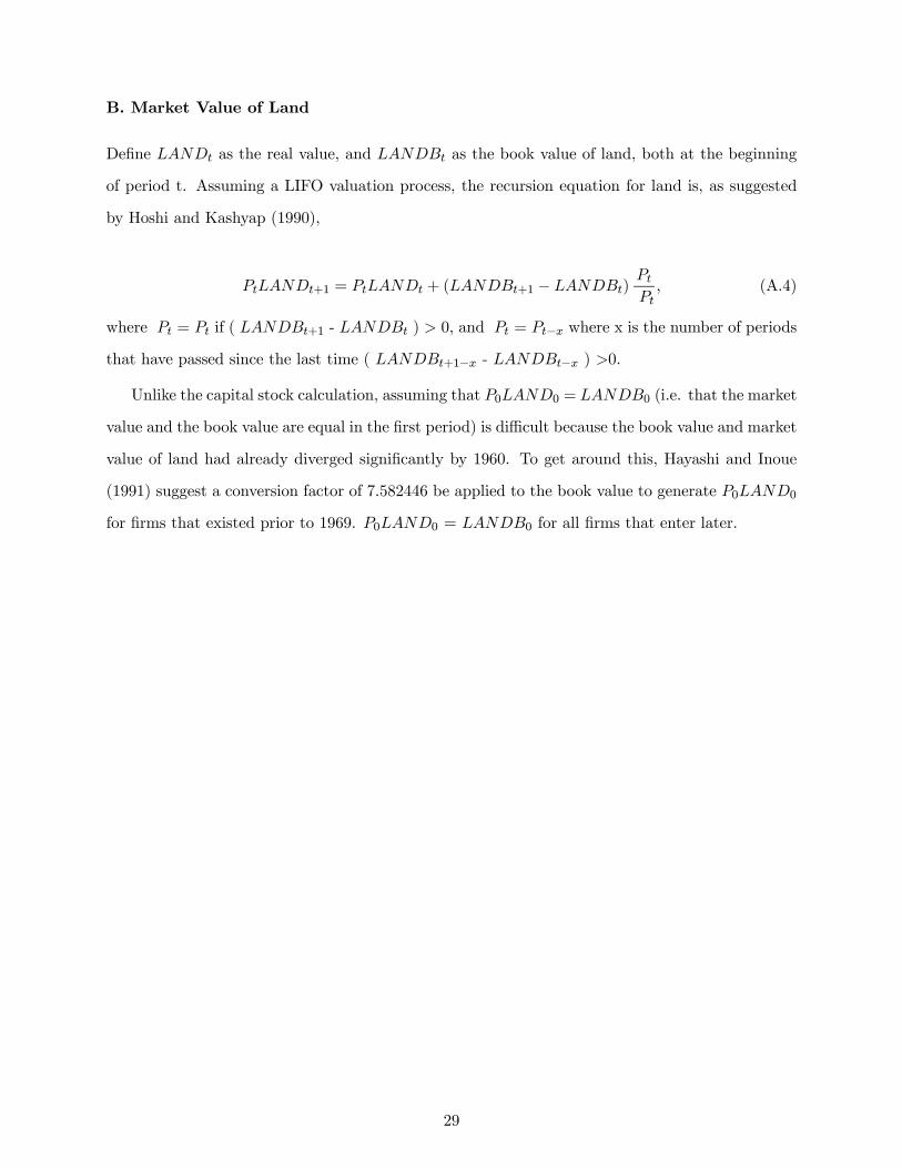
B. Market Value of Land

Define LANDt as the real value, and LANDBt as the book value of land, both at the beginning

of period t. Assuming a LIFO valuation process, the recursion equation for land is, as suggested

by Hoshi and Kashyap (1990),

PtLANDt+1 = PtLANDt + (LANDBt+1 − LANDBt) PtPt, (A.4)

where Pt = Pt if ( LANDBt+1 - LANDBt ) > 0, and Pt = Pt−x where x is the number of periods

that have passed since the last time ( LANDBt+1−x - LANDBt−x ) >0.

Unlike the capital stock calculation, assuming that P0LAND0 = LANDB0 (i.e. that the market

value and the book value are equal in the first period) is difficult because the book value and market

value of land had already diverged significantly by 1960. To get around this, Hayashi and Inoue

(1991) suggest a conversion factor of 7.582446 be applied to the book value to generate P0LAND0

for firms that existed prior to 1969. P0LAND0 = LANDB0 for all firms that enter later.

29

REFERENCES

Alti, Aydogan, 2003, How sensitive is investment to cash flow when financing is frictionless?

Journal of Finance 58: 707-722.

Almeida, H. and M. Campello, 2004, Financial constraints, asset tangibility, and corporate

investment, New York University and University of Illinois Working Paper.

Almeida, H., M. Campello, and M. Weisbach, 2004, The cash flow sensitivity of cash, Journal

of Finance 59: 1777-1804.

Baker, M., J. Stein, J. Wurgler, 2003, When does the market matter? stock price and the

investment of equity-dependent firms, forthcoming, Quarterly Journal of Economics.

Berger, A. and G. Udell, 1995, Relationship lending and lines of credit in small firm finance,

Journal of Business 68: 351-381.

Berger, A. and G. Udell, 1990, Collateral, loan quality, and bank risk, Journal of Monetary

Economics 25, 21-42.

Bernanke, B., 2000, Japanese monetary policy: a case of self-induced paralysis?”, in R. Mikitani

and A. Posen, eds., Japan’s Financial Crisis and its Parallels to U.S. Experience, Institute for

International Economics.

Bernanke, B. and M. Gertler, 1989, Agency costs, net worth, and business fluctuations, Amer-

ican Economic Review 79, 14-31.

Bernanke, B. and M. Gertler, 1990, Financial fragility and economic performance, Quarterly

Journal of Economics 105, 87-114.

Bernanke, B. and M. Gertler, 1995, Inside the black box: the credit channel of monetary policy

transmission, Journal of Economics Perspective 9: 27-48.

Bernanke, B., M. Gertler, and S. Gilchrist, 1996, The financial accelerator and the flight to

quality, Review of Economics and Statistics 78: 1-15.

Besanko, D., Thakor, A., Competition, collateral, and sorting equilibria in the credit market,

International Economic Review 28: 671-89.

Braun, M. and B. Larrain, 2004, Finance and the business cycle: international, inter-industry

evidence, The Journal of Finance, forthcoming.

Binks, M., C. Ennew, and G. Reed, 1988, Small business and banks: a two nation perspective,

30

prepared for the Forum of Private Business, UK and the National Federation of Independent

Business, USA.

Blanchard, O., F. Lopez-de-Silanes, and A. Shleifer, 1994, What do firms do with cash windfalls?

Journal of Financial Economics 36: 337-360.

Blanchard, O., C. Rhee, and L. Summers, 1993, The stock market, profit, and investment,

Quaterly Journal of Economics 108: pp. 115-136.

Bond, S. and C. Meghir, 1994, Dynamic investment models and the firm’s financial policy,

Review of Economic Studies 61: 197-222.

Boot, A., A. Thakor, and G. Udell, 1991, Secured lending and default risk: equilibrium analysis,

policy implications, and empirical results, Economic Journal 101,458-472.

Cargill, T., M. Hutchison, T. Ito, 1997, The political economy of Japanese monetary policy.

Cambridge and London: MIT Press.

Chirinko, R. and H. Schaller, 2001, Business fixed investment and ”bubbles”: the Japanese

case, American Economic Review 91: 663-680.

Cochrane, J., 1996, A cross-sectional test of an investment-based asset pricing model, Journal

of Political Economy 104: 572-612.

Cummins, J., K. Hassett, and S. Oliner, 1999, Investment behavior, observable expectations,

and internal funds, mimeo, New York University.

Dasgupta, S. and K. Sengupta, 2004, Financial constraints, hurdle rates, and investment ac-

tivity: implication from a multi-period model, Hong Kong University of Science and Technology

Working Paper.

Davydenko, S. and J. Franks, 2005, Do bankruptcy code matter? A study of defaults in France,

Germany, and the UK, London Business School Working Paper.

Djankov, S., R. La Porta, F. Lopez-de-Silanes, A. Shleifer, 2003, Courts, Quarterly Journal of

Economics 118 : 453-517.

Economist, The, 1994, Capital cost, July 9.

Economist, The, 1998, The Japan puzzle, March 19.

Erickson, T., and T. Whited, 2000, Measurement error and the relationship between investment

and q, Journal of Political Economy 108, 1027-1057.

31

Fazzari, S., G. Hubbard, and B. Petersen, 1988, Financing constraints and corporate investment,

Brooking Papers of Economic Activities, 141-195.

French, K., and J. Poterba, 1991, Were Japanese stock prices too high? Journal of Financial

Economics 29, 337-363.

Fisher, I., 1933, The debt-deflation theory of great depressions, Econometrica 4, 337-357.

Gilchrist and Himmelberg, 1995, Evidence on the role of cash flow for investment, Journal of

Monetary Economics 36, 541-572.

Gomes, J., 2001, Financing investment, American Economic Review 91, 1263-1258.

Goyal V. and T. Yamada, 2003, Asset price shocks, financial constraints, and investment:

evidence from Japan, forthcoming, Journal of Business.

Harhoff, D. and T. Korting, 1998, Lending relationship in Germany — empirical evidence from

survey data, Journal of Banking and Finance 22, 1317-53.

Hayashi, F. and T. Inoue, 1991, The relation between firm growth and Q with multiple capital

goods: theory and evidence from panel data on Japanese firms, Econometrica 59: 731-53.

Hayashi, F. and E. Prescott, 2002, The 1990s in Japan: A lost decade, Review of Economic

Dynamics 5: 206-236.

Heckman, J., 1979, Sample selection bias as a specification error, Econometrica 47: 153-62.

Hibara, Nobu, 2001, What happens in banking crisis? Moral hazard v. credit crunch. Columbia

University Dissertation.

Hoshi, T. and A. Kashyap, 2001, Corporate Financing and Governance in Japan (MIT Press,

Cambridge, MA).

Hoshi, T. and A. Kashyap, 1990, Evidence on q and investment for Japanese firms, Journal of

the Japanese and International Economies 4: 371-400.

Hoshi, T., A. Kashyap, and D. Scharfstein, 1991, Corporate structure, liquidity, and investment:

evidence from Japanese industrial groups, Quarterly Journal of Economics 106: 33-60.

Hoshi, T., A. Kashyap, and D. Scharfstein, 1990, The role of banks in reducing the costs of

financial distress, Journal of Financial Economics 27: 67-88.

Hubbard, R. G., 1998, Capital market imperfections and investment, Journal of Economic

Literature 36: 193-225.

32

Hurst, E. and Lusardi A., 2004, Liquidity constraints, household wealth, and entrepreneurship,

Journal of Political Economy 112: 319-47.

Jensen, M., 1986, Agency costs of free cash flow, corporate finance and takeovers, American

Economic Review Papers and Proceedings 76: 323-29.

Jensen, M. and W. Meckling, 1976, Theory of the firm: managerial behavior, agency costs and

capital structure, Journal of Financial Economics 3, 305-60.

Kaplan, S. and L. Zingales, 1997, Do investment-cash flow sensitivities provide useful measures

of financing constraints? Quarterly Journal of Economics 112: 169-215.

Kaplan, S. and L. Zingales, 2000, Investment-cash flow sensitivities are not useful measures of

financing constraints, Quarterly Journal of Economics 115: 707-12.

Kashyap, S, O. Lamont, and J. Stein, 1994, Credit conditions and the cyclical behavior of

inventories, Quarterly Journal of Economics 109: 565-92.

Kashyap, A., D. Scharfstein, and D. Weil, 1993, The high price of land and the low cost of

capital: theory and evidence from Japan, MIT working paper.

Kiyotaki, N. and J. Moore, 1997, Credit cycles, Journal of Political Economy 105: 211-248.

Kiyotaki, N. and K. West, 1996, Business fixed investment and the recent business cycle in

Japan, National Bureau of Economic Research Working Paper 5546.

Koenker, R. and G. Bassett Jr., 1982, Robust tests for heteroscedasticity based on regression

quantiles, Econometrica 50, 43-61.

Koenker, R. and G. Bassett Jr., 1978, Regression quantiles, Econometrica 46, 33-50.

Koenker, R. and K. Hallock, 2001, Quantile regression, Journal of Economic Perspectives 15,

143-156.

Kwon, Eunkyung, 1998, Monetary policy, land prices, and collateral effects on economic fluc-

tuations: evidence from Japan, Journal of the Japanese and International Economies 12, 175-203.

La Porta, R., F. Lopez-de-Silanes, A. Shleifer, and R. Vishny, 1998, Law and finance, Journal

of Political Economy 106 (6), 1113—1155.

Lamont, O., 1997, Cash flow and investment: Evidence from internal capital markets, Journal

of Finance 52: 83-109.

Lang, L., E. Ofek, and R. Stulz, 1996, Leverage, investment, and firm growth, Journal of

33

Financial Economics 40: 3-29.

Mayer, C., 1990, Financial systems, corporate finance, and economic development, in R.G.

Hubbard, eds., Asymmetric Information, Corporate Finance and Investment, University of Chicago

Press, Chicago, pp. 307-332.

McGuire, P., 2001, Investment-cash flow sensitivity and bond eligibility: new evidence from

Japan, Ph.D. Dissertation, University of Michigan.

Miwa, Y. and M. Ramseyer, 2002, The fable of the keiretsu, Journal of Economics and Man-

agement Strategy 11: 169-224.

Morck, R., R. Vishny, and A. Shleifer, 1990, The stock market and investment: is the market

a sideshow? Brookings Papers on Economic Activity.

Ogawa, K. and K. Suzuki, 2000, Demand for bank loans and investment under borrowing con-

straints: A panel study of Japanese firm data, Journal of the Japanese and International Economies

14: 1-21.

Opler, Pinkowitz, Stulz, and Williamson, 1999, The determinants and implications of corporate

cash holdings, Journal of Financial Economics 52: 3-46.

Petersen, M. and R. Rajan, 1994, The benefits of lending relationships: evidence from small

business data, Journal of Finance 49, 3-37.

Rajan, R., 1992, Insiders and outsiders: the choice between informed and arm’s length debt,

Journal of Finance 47, 1367-1400.

Rajan, R. and A. Winton, 1995, Covenants and Collateral as Incentive to Monitor, Journal of

Finance 50, 1113-1146.

Rauh, J., 2004, Investment and financing constraints: Evidence from the funding of pension

plans, MIT Working Paper.

Sharpe, S., 1990, Asymmetric information, bank lending and implicit contracts: a stylized model

of customer relationships, Journal of Finance 45, 1069-1087.

Shibata, Y., 1995, Coming soon, a whole new bank credit system for Japan. Global Finance,

August, 58-59.

Shimizu, Y., 1992, Problems in the Japanese financial system in the early 1990s, Hitotsubashi

Journal of Commerce and Management 27: 27-49.

34

Shin, H., R. Stulz, 1998, Are internal capital markets efficient? Quarterly Journal of Economics,

113: 531-52.

Stein, J., 1996, Rational capital budgeting in an irrational world, Journal of Business 69: 429-

455.

Stiglitz, J. and A. Weiss, 1981, Credit rationing in markets with imperfect information, Amer-

ican Economic Review 71, 393-410.

Stulz, R. and H. Johnson, 1985, An analysis of secured debt, Journal of Financial Economics

14, 501-512.

Wall Street Journal, The, 2005, Mailbag: the housing market, June 1.

Weinstein, D. and Y. Yafeh, 1998, On the costs of a bank-centered financial system: evidence

from the changing main bank relations in Japan, The Journal of Finance 53, 635-672.

Whited, 1992, Debt, liquidity constraints, and corporate investment, Journal of Finance 47,

1425-1459.

35

Table I. Summary Statistics

Raw statistics The Whole Sample Land-holding companies The Control Group

(1) (2) (3)Sales ($mil) 165.47 37.58*** 149.95

(48.62) (-5.79)*** (15.04)Cash flow / K 0.08 0.17 0.00

(0.03) (-0.01) (-0.01)Cash / K 1.23 1.94** 0.24

(0.55) (0.26)*** (-0.03)EBDIT / Total assets 0.03 -0.01* 0.00

(0.03) (0.00) (0.00)I / K 0.24 0.46 0.07

(0.09) (0.01)** (0.02)Debt / Total assets 0.12 0.00** 0.02

(0.11) (-0.01)*** -0.01Bank debt / Debt 0.56 -0.02*** -0.10

(0.59) (0.03)*** (-0.11)Tobin's q 0.99 0.06*** 0.35

(0.74) (-0.15)*** (0.12)Number of firms 847 212 635

This table presents descriptive statistics on various firm characteristics in Japan. Column (1)presents the whole-sample summary statistics averaged over the sample period between 1994 and1998. Columns (2) and (3) present the industry-adjusted statistics (adjusted by the median) for thesub-samples of land-holding companies and the control group. The table presents the mean of eachcharacteristic, with the median in the parentheses. Land-holding companies are defined as thecompanies with market value of land to total replacement cost of capital above the industry topquartile. The remaining firms serve as the control group. Significance levels for the differencebetween the landholdingcompanies and the control groups are based on two-tailed tests; significanceat the 1%, 5%, and 10% levels is indicated by ***, **, and *, respectively.

Statistics adjusted by the industry median

36

(1) (2) (3) (4) (5) Cash flow / K 0.415*** 0.216*** 0.142*** 0.126*** 0.146***

(0.021) (0.024) (0.033) (0.032) (0.039) q 0.019*** 0.005*** 0.019*** 0.019*** 0.019***

(0.000) (0.000) (0.000) (0.000) (0.001)Land / Kpre -0.128*** -0.165*** -0.142*** -0.153*** -0.138***

(0.017) (0.016) (0.024) (0.023) (0.028)Cash flow * Landco 0.569*** 0.717*** 0.759*** 0.783*** 0.761***

(0.021) (0.025) (0.034) (0.033) (0.040)Cash/K 0.027*** 0.023*** 0.027*** 0.022***

(0.004) (0.005) (0.005) (0.006)Cash * Landco 0.102*** 0.169*** 0.162*** 0.160***

(0.004) (0.005) (0.005) (0.007)% Recent purchase 0.002 0.039 0.014

(0.042) (0.041) (0.051)% Recent purchase * Landco -0.708*** -0.759*** -0.752***

(0.109) (0.105) (0.126)Leverage 0.008 0.01

(0.033) (0.040)Land / Kpre * High Debt-to-Land -0.025* -0.019

(0.015) (0.018)I_Kpre 0.019***

(0.006)Industry dummies Yes Yes Yes Yes YesNumber of observations 824 751 708 708 708Psuso R2 0.137 0.243 0.311 0.312 0.312

Collateral Effects on Fixed Investments: Basic ResultsTable II.

This table presents the effect of loss of collateral on firm investments based on Least Absolute Distance(LAD) Regressions. The dependent variable I/K is the average investment rate (defined as fixedinvestments over the beginning-of-period capital stock) between 1994 and 1998. Cash flow / K is cashflow over the beginning-of-period capital stock. q is Tobin's average q, Land/Kpre is the market value ofland over the replacement cost of capital in 1989. Landco is a dummy variable equal to 1 if Land/Kpre is above the top industry quartile and 0 otherwise. Cash/K is the cash stock over the beginning-of-periodcapital stock at the end of 1993. % Recent purchase is the proportion of land (in market value) purchasedduring 1988-1990. High Debt-to-Land is a dummyvariable indicating firms with debt over market value ofland in 1989 above the top quartile. I / Kpre is the investment rate prior to the shock in 1989. Standarderrors are based on the asymptotic variance in Koenker and Bassett (1982) and are presented inparentheses.

37

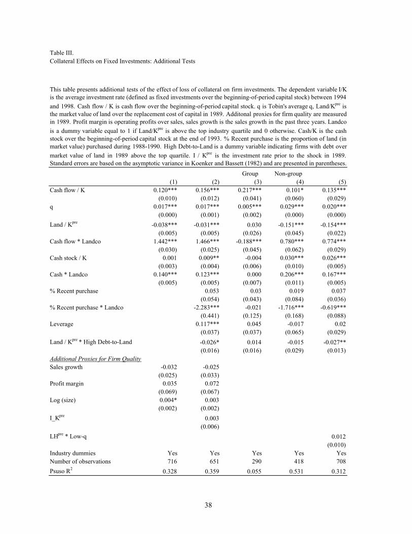
Group Non-group(1) (2) (3) (4) (5)

Cash flow / K 0.120*** 0.156*** 0.217*** 0.101* 0.135***(0.010) (0.012) (0.041) (0.060) (0.029)

q 0.017*** 0.017*** 0.005*** 0.029*** 0.020***(0.000) (0.001) (0.002) (0.000) (0.000)

Land / Kpre -0.038*** -0.031*** 0.030 -0.151*** -0.154***(0.005) (0.005) (0.026) (0.045) (0.022)

Cash flow * Landco 1.442*** 1.466*** -0.188*** 0.780*** 0.774***(0.030) (0.025) (0.045) (0.062) (0.029)

Cash stock / K 0.001 0.009** -0.004 0.030*** 0.026***(0.003) (0.004) (0.006) (0.010) (0.005)

Cash * Landco 0.140*** 0.123*** 0.000 0.206*** 0.167***(0.005) (0.005) (0.007) (0.011) (0.005)

% Recent purchase 0.053 0.03 0.019 0.037(0.054) (0.043) (0.084) (0.036)

% Recent purchase * Landco -2.283*** -0.021 -1.716*** -0.619***(0.441) (0.125) (0.168) (0.088)

Leverage 0.117*** 0.045 -0.017 0.02(0.037) (0.037) (0.065) (0.029)

Land / Kpre * High Debt-to-Land -0.026* 0.014 -0.015 -0.027**(0.016) (0.016) (0.029) (0.013)

Additional Proxies for Firm QualitySales growth -0.032 -0.025

(0.025) (0.033)Profit margin 0.035 0.072

(0.069) (0.067)Log (size) 0.004* 0.003

(0.002) (0.002)I_Kpre 0.003

(0.006)LHpre * Low-q 0.012

(0.010)Industry dummies Yes Yes Yes Yes YesNumber of observations 716 651 290 418 708Psuso R2 0.328 0.359 0.055 0.531 0.312

Table III.Collateral Effects on Fixed Investments: Additional Tests

This table presents additional tests of the effect of loss of collateral on firm investments. The dependent variable I/Kis the average investment rate (defined as fixed investments over the beginning-of-period capital stock) between 1994and 1998. Cash flow / K is cash flow over the beginning-of-period capital stock. q is Tobin's average q, Land/Kpre isthe market value of land over the replacement cost of capital in 1989. Additonal proxies for firm quality are measuredin 1989. Profit margin is operating profits over sales, sales growth is the sales growth in the past three years. Landcois a dummy variable equal to 1 if Land/Kpre is above the top industry quartile and 0 otherwise. Cash/K is the cashstock over the beginning-of-period capital stock at the end of 1993. % Recent purchase is the proportion of land (inmarket value) purchased during 1988-1990. High Debt-to-Land is a dummy variable indicating firms with debt overmarket value of land in 1989 above the top quartile. I / Kpre is the investment rate prior to the shock in 1989.Standard errors are based on the asymptotic variance in Koenker and Bassett (1982) and are presented in parentheses.

38

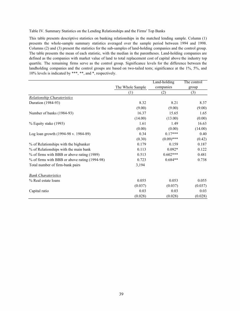
Table IV. Summary Statistics on the Lending Relationships and the Firms' Top Banks

The Whole SampleLand-holding

companiesThe control

group(1) (2) (3)

Relationship CharateristicsDuration (1984-93) 8.32 8.21 8.37

(9.00) (9.00) (9.00)Number of banks (1984-93) 16.37 15.65 1.65

(14.00) (13.00) (0.00)% Equity stake (1993) 1.61 1.49 16.63

(0.00) (0.00) (14.00)Log loan growth (1994-98 v. 1984-89) 0.34 0.17*** 0.40

(0.30) (0.09)*** (0.42)% of Relationships with the bigbanker 0.179 0.159 0.187% of Relationships with the main bank 0.113 0.092* 0.122% of firms with BBB or above rating (1989) 0.513 0.602*** 0.481% of firms with BBB or above rating (1994-98) 0.723 0.684** 0.738Total number of firm-bank pairs 3,194

Bank Charateristics% Real estate loans 0.055 0.053 0.055

(0.037) (0.037) (0.037) Capital ratio 0.03 0.03 0.03

(0.028) (0.028) (0.028)

This table presents descriptive statistics on banking relationships in the matched lending sample. Column (1)presents the whole-sample summary statistics averaged over the sample period between 1994 and 1998.Columns (2) and (3) present the statistics for the sub-samples of land-holding companies and the control group.The table presents the mean of each statistic, with the median in the parentheses. Land-holding companies aredefined as the companies with market value of land to total replacement cost of capital above the industry topquartile. The remaining firms serve as the control group. Significance levels for the difference between thelandholding companies and the control groups are based on two-tailed tests; significance at the 1%, 5%, and10% levels is indicated by ***, **, and *, respectively.

39

Table VCollateral Effects on Corporate Borrowing

(1a) (1b) (2a) (2b)Probit OLS Probit OLS

Relationship CharacteristicsDuration (1984-89) 0.193*** -0.421*** 0.193*** -0.403***

(0.013) (0.040) (0.013) (0.038)Number of banks (1984-89) 0.007 -0.015 0.017 -0.024

(0.078) (0.079) (0.078) (0.078)Bigbanker (1984-89) 0.457*** -0.082 0.454*** -0.060

(0.097) (0.083) (0.096) (0.082)Equity ownership 0.094*** 0.033* 0.094*** 0.039**

(0.021) (0.019) (0.021) (0.019)Main Bank 0.113 -0.120 0.123 -0.112

(0.102) (0.089) (0.103) (0.089)Access to Bond Market 0.131*** -0.039

(0.050) (0.063)Firm CharacteristicsLog of assets -0.044 -0.041 -0.039 -0.041

(0.032) (0.032) (0.032) (0.032)q -0.106*** 0.001 -0.112*** 0.001

(0.023) (0.002) (0.023) (0.002)Cash flow/K 0.144** 0.103 0.131* 0.103

(0.067) (0.131) (0.067) (0.130)Cash/K -0.025* -0.017 -0.023* -0.017

(0.013) (0.022) (0.013) (0.021)Collateral Related VariablesLand/Kpre -0.240* -0.487*** -0.294** -0.494***

(0.135) (0.187) (0.132) (0.188)% Recent purchase 4.100*** 1.051 4.154*** 1.265*

(1.050) (0.729) (1.072) (0.732)% Recent purchase * Landco 1.026 -3.570 1.133 -3.507

(3.043) (3.387) (3.140) (3.407)Inverse Mills Ratio -1.247*** -1.022**

(0.472) (0.454)Number of observations 3191 2626 3191 2626Psuso R2 / R2 0.162 0.300 0.164 0.300

This table presents the effectof collateral losses on bank lending based on Heckman two-stage regressions. The first stageis a probit regression. The dependent variable is a dummy variable indicating the survival of the lending relationship. q isTobin's average q. Cash flow/K is cash flow over the beginning-of-periodcapital stock. Cash/K is the cash stock over thecapital stock at the end of 1993. Duration is the number of years that the firm-bank pair had positive loan balances. Bigbanker is whether the bank served as the firm's largest lender at least once. Main bank is a dummy variable equals to 1 ifthe bank is also the firm's main bank and zero otherwise. Equity ownership is the percent of shares owned by the bank.Number of banks is the number of banks with which the firm had lending relationships. Land/Kpre is the market value ofland over the capital stock in 1990. Landco is a dummy variable equals to 1 if Land/Kpre is above the top quartile in theindustry and 0 otherwise. Robust standard errors are presented in parentheses.

40

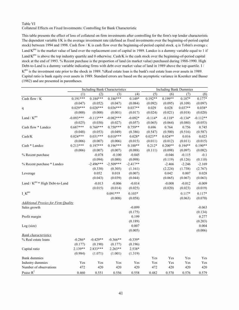
(1) (2) (3) (4) (5) (6) (7) (8) Cash flow / K 0.191*** 0.184*** 0.186*** 0.149* 0.192** 0.199** 0.187* 0.177*

(0.047) (0.052) (0.047) (0.084) (0.092) (0.095) (0.109) (0.097) q 0.029*** 0.028*** 0.036*** 0.037** 0.029 0.028 0.037** 0.038*

(0.000) (0.000) (0.001) (0.017) (0.024) (0.021) (0.018) (0.020) Land / Kpre -0.093*** -0.113*** -0.082*** -0.092* -0.114* -0.118* -0.134* -0.112**

(0.025) (0.030) (0.027) (0.057) (0.065) (0.064) (0.080) (0.053) Cash flow * Landco 0.687*** 0.760*** 0.750*** 0.759** 0.696 0.764 0.756 0.745

(0.048) (0.053) (0.049) (0.386) (0.547) (0.500) (0.516) (0.587) Cash/K 0.024*** 0.031*** 0.018*** 0.028* 0.023** 0.024** 0.016 0.023

(0.006) (0.007) (0.006) (0.015) (0.011) (0.012) (0.011) (0.015) Cash * Landco 0.213*** 0.197*** 0.196*** 0.188** 0.212* 0.200** 0.194** 0.190**

(0.006) (0.007) (0.007) (0.088) (0.111) (0.098) (0.097) (0.082) % Recent purchase -0.078 -0.100 -0.045 -0.046 -0.115 -0.1

(0.094) (0.088) (0.098) (0.119) (0.126) (0.110) % Recent purchase * Landco -2.496*** -2.509*** -2.417** -2.466 -2.246 -2.169

(0.338) (0.305) (1.161) (2.224) (1.738) (2.767) Leverage 0.052 0.018 (0.007) 0.042 0.007 0.028

(0.043) (0.039) (0.044) (0.065) (0.067) (0.063) Land / Kpre * High Debt-to-Land -0.013 -0.006 -0.014 -0.008 -0.012 -0.009

(0.015) (0.014) (0.025) (0.020) (0.023) (0.019) I_Kpre 0.091*** 0.103* 0.117* 0.117*

(0.008) (0.058) (0.063) (0.070) Additional Proxies for Firm QualitySales growth -0.099 -0.063

(0.175) (0.134) Profit margin 0.199 0.277

(0.189) (0.203) Log (size) 0.007 0.004

(0.005) (0.006) Bank characteristics% Real estate loans -0.286* -0.429** -0.366** -0.339*

(0.177) (0.190) (0.177) (0.196) Capital ratio 2.139** 2.833*** 2.263** 2.538*

(0.984) (1.071) (1.001) (1.319) Bank dummies Yes Yes Yes YesIndustry dummies Yes Yes Yes Yes Yes Yes Yes YesNumber of observations 472 420 420 420 472 420 420 420Psuso R2 0.460 0.551 0.556 0.558 0.482 0.570 0.576 0.579

Including Bank Characteristics Including Bank Dummies

This table presents the effect of loss of collateral on firm investments after controlling for the firm's top lender characteristicThe dependent variable I/K is the average investment rate (defined as fixed investments over the beginning-of-period capital stock) between 1994 and 1998. Cash flow / K is cash flow over the beginning-of-period capital stock. q is Tobin's average qLand/Kpre is the market value of land over the replacement cost of capital in 1989. Landco is a dummy variable equal to 1 if Land/Kpre is above the top industry quartile and 0 otherwise. Cash/K is the cash stock over the beginning-of-period capital stock at the end of 1993. % Recent purchase is the proportion of land (in market value) purchased during 1988-1990. High Debt-to-Land is a dummy variable indicating firms with debt over market value of land in 1989 above the top quartile. I / Kpre is the investment rate prior to the shock in 1989. %Real estate loan is the bank's real estate loan over assets in 1989. Capital ratio is bank equity over assets in 1989. Standard errors are based on the asymptotic variance in Koenker and Basset(1982) and are presented in parentheses.

Table VICollateral Effects on Fixed Investments: Controlling for Bank Characteristic

41