Collaborative Place ModelsBerk KapiciogluFoursquare Labs

berk.kapicioglu@gmail.com

David S. RosenbergYP Mobile Labs

david.davidr@gmail.com

Robert E. SchapirePrinceton University

schapire@cs.princeton.edu

Tony JebaraColumbia University

jebara@cs.columbia.edu

AbstractA fundamental problem underlying location-basedtasks is to construct a complete profile of users’spatiotemporal patterns. In many real-world set-tings, the sparsity of location data makes it diffi-cult to construct such a profile. As a remedy, wedescribe a Bayesian probabilistic graphical model,called Collaborative Place Model (CPM), which in-fers similarities across users to construct completeand time-dependent profiles of users’ whereaboutsfrom unsupervised location data. We apply CPMto both sparse and dense datasets, and demonstratehow it both improves location prediction perfor-mance and provides new insights into users’ spa-tiotemporal patterns.

1 Introduction1

During the last couple of years, positioning devices that mea-sure and record our locations have become ubiquitous. Themost common positioning device, the smartphone, is pro-jected to be used by a billion people in the near future [Davie,2012]. This surge in positioning devices has increased theavailability of location data, and provided scientists with newresearch opportunities, such as building location-based rec-ommendation systems [Hao et al., 2010; Zheng et al., 2010;2009], analyzing human mobility patterns [Brockmann et al.,2006; Gonzalez et al., 2008; Song et al., 2010], and modelingthe spread of diseases [Eubank et al., 2004].

A fundamental problem underlying many location-basedtasks is modeling users’ spatiotemporal patterns. For exam-ple, a navigation application that has access to traffic condi-tions can warn the user about when to depart, without requir-ing any input from the user, as long as the application canaccurately model user’s destination. Similarly, a restaurantapplication can provide a list of recommended venues, evenreserve them while space is still available, by modeling theprobable locations the user might visit for lunch.

One of the challenges in building such models is thesparsity of location datasets. Due to privacy considerations[Wernke et al., 2012] and high energy consumption of posi-tioning hardware [Oshin et al., 2012], location datasets con-

1Supplements are available at http://www.berkkapicioglu.com.

0 1000 2000 3000 40000

20

40

60

80

100

Number of observations per user (dense dataset)Mean: 1172.2, Median: 1114.0

Number of observations

Nu

mb

er

of

use

rs

0 200 400 600 800 10000

1000

2000

3000

4000

Number of observations per user (sparse dataset)Mean: 107.3, Median: 74.0

Number of observations

Nu

mb

er

of

use

rs

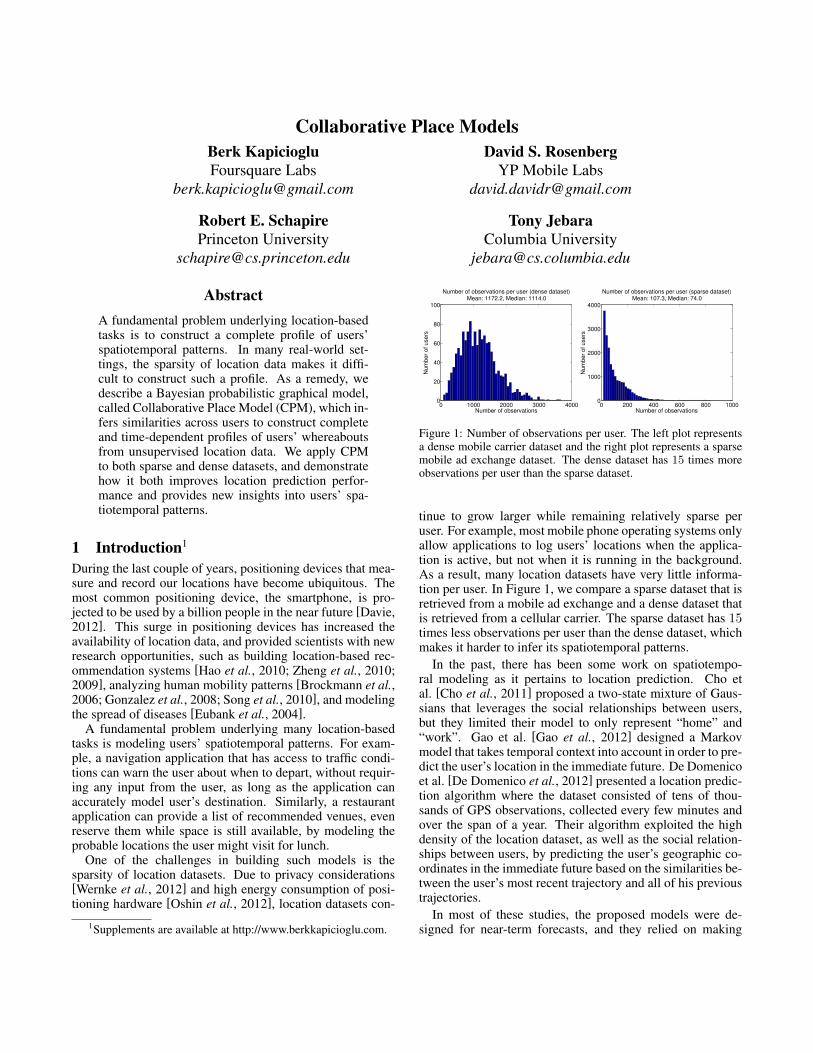
Figure 1: Number of observations per user. The left plot representsa dense mobile carrier dataset and the right plot represents a sparsemobile ad exchange dataset. The dense dataset has 15 times moreobservations per user than the sparse dataset.

tinue to grow larger while remaining relatively sparse peruser. For example, most mobile phone operating systems onlyallow applications to log users’ locations when the applica-tion is active, but not when it is running in the background.As a result, many location datasets have very little informa-tion per user. In Figure 1, we compare a sparse dataset that isretrieved from a mobile ad exchange and a dense dataset thatis retrieved from a cellular carrier. The sparse dataset has 15times less observations per user than the dense dataset, whichmakes it harder to infer its spatiotemporal patterns.

In the past, there has been some work on spatiotempo-ral modeling as it pertains to location prediction. Cho etal. [Cho et al., 2011] proposed a two-state mixture of Gaus-sians that leverages the social relationships between users,but they limited their model to only represent “home” and“work”. Gao et al. [Gao et al., 2012] designed a Markovmodel that takes temporal context into account in order to pre-dict the user’s location in the immediate future. De Domenicoet al. [De Domenico et al., 2012] presented a location predic-tion algorithm where the dataset consisted of tens of thou-sands of GPS observations, collected every few minutes andover the span of a year. Their algorithm exploited the highdensity of the location dataset, as well as the social relation-ships between users, by predicting the user’s geographic co-ordinates in the immediate future based on the similarities be-tween the user’s most recent trajectory and all of his previoustrajectories.

In most of these studies, the proposed models were de-signed for near-term forecasts, and they relied on making

predictions based on the most recent observations. However,there are many real-world applications where the test exam-ple and the most recent training example are temporally apart,and for all purposes, statistically independent. For such pre-dictions, a model that relies on the most recent observationswould not suffice; instead, the model would need to make pre-dictions based on the user’s global spatiotemporal patterns.

In addition to the work listed above, researchers have alsostudied spatiotemporal modeling as it pertains to the detectionof significant places and routines. Eagle and Pentland [Ea-gle and Pentland, 2009] applied eigendecomposition to theReality Mining dataset, where all locations were already la-beled as “home” or “work”, and extracted users’ daily rou-tines. Farrahi and Gatica-Perez [Farrahi and Perez, 2011]used the same dataset, but extracted the routines using LatentDirichlet Allocation (LDA) instead of eigendecomposition.Liao et al. [Liao et al., 2005; 2007] proposed a hierarchicalconditional random field to identify activities and significantplaces from the users’ GPS traces, and since their algorithmwas supervised, it required locations to be manually labeledfor training. In contrast to previous work, our model doesnot require labeled data; instead, it relies only on user IDs,latitudes, longitudes, and time stamps.

In this paper, we propose a new Bayesian probabilisticgraphical model, called Collaborative Place Model (CPM),which recovers the latent spatiotemporal structure underly-ing unsupervised location data by analyzing patterns sharedacross all users. CPM is a generalization of the BayesianGaussian mixture model (GMM), and assumes that each useris characterized by a varying number of place clusters, whosespatial characteristics, such as their means and covariances,are determined probabilistically from the data. However, un-like GMM, CPM also assigns users weakly similar temporalpatterns; ones which do not force different users to have thesame place distribution during the same weekhour.

The spatiotemporal patterns extracted by CPM are helpfulin leveraging both sparse and dense datasets. In case of sparsedata, the model infers a user’s place distribution at a particu-lar weekhour, even if the user has not been observed duringthat weekhour before. In case of dense data, sampling biasusually yields fewer observations for certain hours (e.g. usersmake more phone calls during day time than after midnight),and the model successfully infers the user’s behavior duringthese undersampled hours. In both cases, the model combinesthe globally shared temporal patterns with user’s own spa-tiotemporal patterns and constructs a customized, complete,and time-dependent profile of the user’s locations.

Aside from its quantitative benefits, CPM also providesqualitative insights about the universal temporal patterns ofhuman populations. Even though the model is given no priorinformation about the relationship between weekhours, it suc-cessfully extracts temporal clusters such as the hours spentduring morning commute, work, evening commute, leisuretime after work, and sleeping at night.

The paper proceeds as follows. In Section 2, we provide aformal description of CPM. In Section 3, we derive the infer-ence algorithms. In Section 4, we demonstrate our model ontwo real location datasets. We conclude in Section 5.

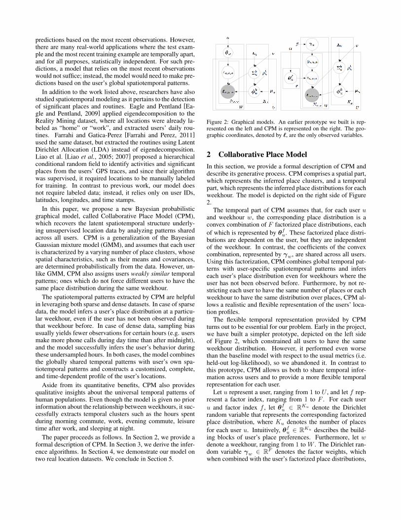
Figure 2: Graphical models. An earlier prototype we built is rep-resented on the left and CPM is represented on the right. The geo-graphic coordinates, denoted by �, are the only observed variables.

2 Collaborative Place ModelIn this section, we provide a formal description of CPM anddescribe its generative process. CPM comprises a spatial part,which represents the inferred place clusters, and a temporalpart, which represents the inferred place distributions for eachweekhour. The model is depicted on the right side of Figure2.

The temporal part of CPM assumes that, for each user uand weekhour w, the corresponding place distribution is aconvex combination of F factorized place distributions, eachof which is represented by θf

u. These factorized place distri-butions are dependent on the user, but they are independentof the weekhour. In contrast, the coefficients of the convexcombination, represented by γw, are shared across all users.Using this factorization, CPM combines global temporal pat-terns with user-specific spatiotemporal patterns and inferseach user’s place distribution even for weekhours where theuser has not been observed before. Furthermore, by not re-stricting each user to have the same number of places or eachweekhour to have the same distribution over places, CPM al-lows a realistic and flexible representation of the users’ loca-tion profiles.

The flexible temporal representation provided by CPMturns out to be essential for our problem. Early in the project,we have built a simpler prototype, depicted on the left sideof Figure 2, which constrained all users to have the sameweekhour distribution. However, it performed even worsethan the baseline model with respect to the usual metrics (i.e.held-out log-likelihood), so we abandoned it. In contrast tothis prototype, CPM allows us both to share temporal infor-mation across users and to provide a more flexible temporalrepresentation for each user.

Let u represent a user, ranging from 1 to U , and let f rep-resent a factor index, ranging from 1 to F . For each useru and factor index f , let θf

u ∈ RKu denote the Dirichletrandom variable that represents the corresponding factorizedplace distribution, where Ku denotes the number of placesfor each user u. Intuitively, θf

u ∈ RKu describes the build-ing blocks of user’s place preferences. Furthermore, let wdenote a weekhour, ranging from 1 to W . The Dirichlet ran-dom variable γw ∈ RF denotes the factor weights, whichwhen combined with the user’s factorized place distributions,

yields the user’s place distribution for weekhour w.At a high level, the generative process proceeds as follows.

The variable γw generates yu,w,n, the factor assignment foruser u and observation n at weekhour w, and the factor as-signment generates the place assignment zu,w,n from the fac-torized place distribution θyu,w,n

u . The place assignment is inturn used to sample the observed coordinates �u,w,n from thecorresponding place cluster.

The place clusters, whose means and covariances areunique to each user, are modeled by the spatial part of CPM.Intuitively, we expect each place cluster to correspond to lo-cations such as “home”, “work”, and “gym”. Given a user uand a place index k, each place cluster is characterized by abivariate normal distribution, with mean φk

u and covarianceΣk

u. The observed coordinates � are considered to be noisyobservations sampled from these place clusters.

Our model uses conjugate priors because of the compu-tational advantages they provide in Bayesian inference. Forthe random variables θf

w and γw, the prior is a symmet-ric Dirichlet with concentration parameter α > 0, whereDirichletK (α) denotes the K-dimensional distribution. Forthe random variables associated with the place clusters, φk

u

and Σku, the prior is a normal-inverse-Wishart (NIW) distri-

bution. Λ ∈ R2×2 is a positive definite scale matrix, ν>1indicates the degrees of freedom, and together they define thedistribution over the covariance matrix. The parameter µu iscustomized for each user u and is computed as the mean ofthe user’s historical locations. The parameter puk is set suchthat the prior covariance of the place mean (i.e. prior covari-ance of φk

u) is very large.In location datasets, a user sometimes logs locations that

are one-offs and are not representative of the user’s regular lo-cation profile. To ensure that such outliers do not affect howthe model infers the user’s regular place clusters, we desig-nate the last place, place Ku, as a special outlier place and setits covariance’s prior mean (i.e. prior mean of ΣKu

u ), as de-termined by ΛKu , to be very large. As for the covariance ofregular clusters, we set the remaining scale matrices, Λ−Ku ,such that each coordinate of the covariance’s prior mean hasa standard deviation of 150 meters. This is a reasonable sizefor a place cluster, as it is large enough to encapsulate boththe potential inaccuracies of location hardware and the inher-ent noise in the users’ locations, but small enough to ensurethat each place cluster corresponds to a single intuitive place,such as “home” or “work”.

Let N denote the normal distribution and IW denote theinverse-Wishart distribution. Let DirichletK (·) denote a sym-metric Dirichlet if its parameter is a scalar and a generalDirichlet if its parameter is a vector. The generative processof CPM is described in more formal terms below. Furthertechnical details about the distributions we use in our modelcan be found in the supplement.

1. For each weekhour w, draw a distribution over factorsγw ∼ DirichletF (β).

2. For each user u and factor f , draw a factorized placedistribution θf

u ∼ DirichletKu (α).3. For each user u and place k,

(a) Draw a place covariance Σku ∼ IW (Λk, ν).

(b) Draw a place mean φku ∼ N

�µu,

Σku

puk

�.

4. For each user u, weekhour w, and observation index n,

(a) Draw a factor assignmentyu,w,n ∼ Categorical(γw).

(b) Draw a place assignmentzu,w,n ∼ Categorical(θyu,w,n

u ).(c) Draw a location

�u,w,n ∼ N (φzu,w,nu ,Σzu,w,n

u ).

3 InferenceIn this section, we derive our inference algorithm, and wepresent our derivation in multiple steps. First, we derive acollapsed Gibbs sampler to sample from the posterior distri-bution of the categorical random variables conditioned on theobserved geographic coordinates. Second, we derive the con-ditional likelihood of the posterior samples, which we useto determine the sampler’s convergence. Third, we deriveformulas for approximating the posterior expectations of thenon-categorical random variables conditioned on the poste-rior samples. Finally, in the last step, we combine all theprevious derivations to construct a simple algorithm for ef-ficient posterior inference. We state the main results below.The proofs are provided in the supplement.

In Lemmas 1 and 2, we describe the collapsed Gibbs sam-pler for variables z and y, respectively. Given a vector x andan index k, let x−k indicate all the entries of the vector ex-cluding the one at index k. We assume that i = (u,w, n)denotes the index of the variable that will be sampled. First,we state the posterior probability of z.

Lemma 1. The unnormalized probability of zi conditionedon the observed location data and remaining categoricalvariables is

p�zi = k | yi = f, z−i,y−i, �

�

∝ tvuk−1

��i | µu

k ,Λ

ku (p

uk + 1)

puk (vuk − 1)

��α+ mk,f

u,·�.

The parameters vuk , µuk , Λ

ku, and puk are defined in the proof. t

denotes the bivariate t-distribution and mk,fu,· denotes counts,

both of which are defined in the supplement.

Next, we state the posterior probability of y.

Lemma 2. The unnormalized probability of yi conditionedon the observed location data and remaining categoricalvariables is

p�yi = f | zi = k,y−i, z−i, �

�

∝ α+ mk,fu,·

Kuα+ m·,fu,·

�βw,f + m·,f

·,w�,

where the counts mk,fu,· , m·,f

u,·, and m·,f·,w are defined in the

supplement.

In Lemma 3, we describe the conditional log-likelihoods ofthe posterior samples conditioned on the observed geograph-ical coordinates. We use these conditional log-likelihoodsto determine the sampler’s convergence. Later in the paper,when we present the algorithm for posterior inference, wewill use these conditional likelihoods to determine the algo-rithm’s convergence. Let Γ denote the gamma function, letΓ2 denote the bivariate gamma function, and let |·| denote thedeterminant.Lemma 3. The log-likelihood of the samples z and y condi-tioned on the observations � is

log p (z,y | �) =

W�

w=1

F�

f=1

logΓ�βw,f +m·,f

·,w�

+

U�

u=1

F�

f=1

− logΓ�αKu +m·,f

u,·�

+

U�

u=1

F�

f=1

Ku�

k=1

logΓ�α+mk,f

u,·�

+

�U�

u=1

Ku�

k=1

�logΓ2

�vuk2

�−mk,·

u,· log π

��

+

�U�

u=1

Ku�

k=1

�− vuk

2log

���Λk

u

���− log puk

��+ C,

where C denotes the constant terms. The counts m·,f·,w, m·,f

u,·,mk,·

u,·, and mk,fu,· are defined in the supplement. The parame-

ters vuk , Λk

u, and puk are defined in the proof.In Lemmas 1 and 2, we described a collapsed Gibbs sam-

pler for sampling the posteriors of the categorical randomvariables. In Lemma 4, we show how these samples, denotedas y and z, can be used to approximate the posterior expecta-tions of γ, θ, φ, and Σ.Lemma 4. The expectations of γ, θ, φ, and Σ given theobserved geographical coordinates and the posterior samplesare

γw,f = E [γw,f | y, z, �] = βw,f +m·,f·,w

�f

�βw,f +m·,f

·,w

� ,

θfu,k = E�θfu,k | y, z, �

�=

α+mk,fu,·

Kuα+m·,fu,·

,

φk

u = E�φk

u | y, z, ��= µu

k ,

Σk

u = E�Σk

u | y, z, ��=

Λk

u

vuk − 3.

Counts m·,f·,w, mk,f

u,· , and m·,fu,· are defined in the supplement.

Parameters µuk , Λ

k

u, and vuk are defined in the proof.Finally, we combine our results to construct an algorithm

for efficient posterior inference. The algorithm uses Lemmas

Algorithm 1 Collapsed Gibbs sampler for CPM.Input: Number of factors F , number of places Ku, hyperpa-

rameters α, β, ν, pk, Λk, and µu.1: Initialize y and z uniformly at random.2: Initialize mk,f

u,· , m·,fu,·, m·,f

·,w, mk,·u,·, Su

k , and P uk based on

y and z.3: while the log-likelihood in Lemma 3 has not

converged do4: Choose index i = (u,w, n) uniformly at random.5: mzi,yi

u,· ← mzi,yiu,· − 1, m·,yi

u,· ← m·,yiu,· − 1,

m·,yi·,w ← m·,yi

·,w − 1.6: Sample yi with respect to Lemma 2.7: mzi,yi

u,· ← mzi,yiu,· + 1, m·,yi

u,· ← m·,yiu,· + 1,

m·,yi·,w ← m·,yi

·,w + 1.8: Choose index i = (u,w, n) uniformly at random.9: mzi,yi

u,· ← mzi,yiu,· − 1, mzi,·

u,· ← mzi,·u,· − 1,

Suzi ← Su

zi − �i, P uzi ← P u

zi − �i�Ti .

10: Sample zi with respect to Lemma 1.11: mzi,yi

u,· ← mzi,yiu,· + 1, mzi,·

u,· ← mzi,·u,· + 1,

Suzi ← Su

zi + �i, P uzi ← P u

zi + �i�Ti .

12: Compute γ, θ, φ, and Σ using Lemma 4.13: return γ, θ, φ, and Σ.

1 and 2 to implement the collapsed Gibbs sampler, Lemma 3to determine convergence, and Lemma 4 to approximate theposterior expectations. The sufficient statistics are defined inthe supplement.

4 ExperimentsIn this section, we demonstrate the performance of CPMon two real-world location datasets, a dense cellular carrierdataset and a sparse mobile ad exchange dataset, both ofwhich are depicted in Figure 1.

We start by describing how we set up the experiments.Each data point consists of a user ID, a local time, and ge-ographic coordinates represented as latitudes and longitudes.First, we check if a user has logged multiple observations dur-ing the same hour, and if so, we replace these observationswith their geometric median, computed using Weiszfeld’s al-gorithm. Since geometric median is a robust estimator, thisstep removes both noisy and redundant observations. Then,we sort the datasets chronologically, and for each user, splitthe user’s data points into 3 partitions: earliest 60% is addedto the training data, middle 20% to the validation data, andfinal 20% to the test data. After preprocessing, both datasetscontain approximately 2 million data points, the dense datasetcontains 1394 users, and the sparse dataset contains 19247users. Furthermore, since the temporal gap between the train-ing data and the test data ends up being at least a week apart,our datasets become inappropriate for models that make near-term forecasts based on the most recent observations.

We train our model in two stages. In the first stage, we de-termine both the optimal number of places for each user (i.e.Ku) and the optimal setting for each spatial hyperparameter(i.e. ν, pk, Λk, and µu). To do so, we extract the spatialpart of CPM into a GMM and train a different GMM for all

1 2 3 4 5 6 7 8 9 10

!16.38

!16.36

!16.34

!16.32

!16.3

!16.28

Test log!likelihood (dense dataset)

Number of components

Log!

likelih

ood

1 2 3 4 5 6 7 8 9 10

!16.52

!16.5

!16.48

!16.46

!16.44

!16.42

Test log!likelihood (sparse dataset)

Number of components

Log!

likelih

ood

200 400 600 800 100036

38

40

42

44

46

48

Distance (m)

Acc

ura

cy (

%)

Test accuracy (sparse dataset)

CPMGMM

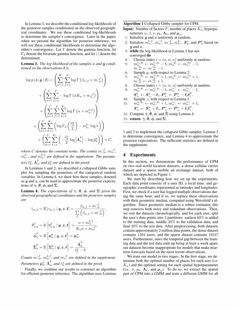
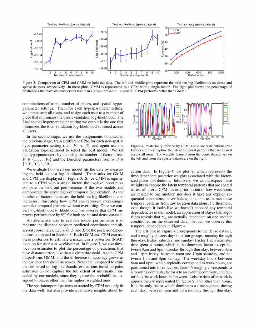
Figure 3: Comparison of CPM and GMM on held-out data. The left and middle plots represent the held-out log-likelihoods on dense andsparse datasets, respectively. In these plots, GMM is represented as a CPM with a single factor. The right plot shows the percentage ofpredictions that have distance errors less than a given threshold. In general, CPM performs better than GMM.

combinations of users, number of places, and spatial hyper-parameter settings. Then, for each hyperparameter setting,we iterate over all users, and assign each user to a number ofplace that minimizes the user’s validation log-likelihood. Thefinal spatial hyperparameter setting we output is the one thatminimizes the total validation log-likelihood summed acrossall users.

In the second stage, we use the assignments obtained inthe previous stage, train a different CPM for each non-spatialhyperparameter setting (i.e. F , α, β), and again use thevalidation log-likelihood to select the best model. We setthe hyperparameters by choosing the number of factors fromF ∈ {1, . . . , 10} and the Dirichlet parameters from α,β ∈{0.01, 0.1, 1, 10}.

We evaluate how well our model fits the data by measur-ing the held-out test log-likelihood. The results for GMMand CPM are displayed in Figure 3. Since GMM is equiva-lent to a CPM with a single factor, the log-likelihood plotscompare the held-out performance of the two models anddemonstrate the advantages of temporal factorization. As thenumber of factors increases, the held-out log-likelihood alsoincreases, illustrating how CPM can represent increasinglycomplex temporal patterns without overfitting. Once we con-vert log-likelihood to likelihood, we observe that CPM im-proves performance by 8% for both sparse and dense datasets.

An alternative way to evaluate model performance is tomeasure the distance between predicted coordinates and ob-served coordinates. Let γ, θ, φ, and Σ be the posterior expec-tations computed in Section 3. Both GMM and CPM can usethese posteriors to estimate a maximum a posteriori (MAP)location for user u at weekhour w. In Figure 3, we use theselocation estimates to plot the percentage of predictions thathave distance errors less than a given threshold. Again, CPMoutperforms GMM, and the difference in accuracy grows asthe distance threshold increases. Note that compared to eval-uations based on log-likelihoods, evaluations based on pointestimates do not capture the full extent of information en-coded by our models, since they ignore the probabilities as-signed to places other than the highest weighted ones.

The spatiotemporal patterns extracted by CPM not only fitthe data well, but also provide qualitative insights about lo-

0 24 48 72 96 120 144 1680

0.2

0.4

0.6

0.8

1

Weekhours

Pro

babili

ty

123456789

0 24 48 72 96 120 144 1680

0.2

0.4

0.6

0.8

1

Weekhours

Pro

babili

ty

12345678910

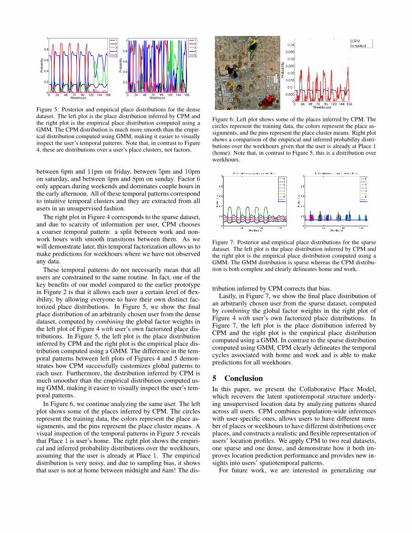
Figure 4: Posterior γ inferred by CPM. These are distributions overfactors and they capture the latent temporal patterns that are sharedacross all users. The weights learned from the dense dataset are onthe left and from the sparse dataset are on the right.

cation data. In Figure 4, we plot γ, which represents thetime-dependent posterior weights associated with the factor-ized place distributions. Intuitively, we would expect theseweights to capture the latent temporal patterns that are sharedacross all users. CPM has no prior notion of how weekhoursare related to one another, nor does it have any explicit se-quential constraints; nevertheless, it is able to extract thesetemporal patterns from raw location data alone. Furthermore,even though it looks like we haven’t encoded any temporaldependencies in our model, an application of Bayes ball algo-rithm reveals that γw are actually dependent on one anotherconditioned on the observed data. In fact, we observe thistemporal dependency in Figure 4.

The left plot in Figure 4 corresponds to the dense dataset,and it roughly clusters days into four groups: monday throughthursday, friday, saturday, and sunday. Factor 1 approximatestime spent at home, which is the dominant factor except be-tween 8am and 8pm monday through thursday, between 8amand 11pm friday, between noon and 10pm saturday, and be-tween 1pm and 8pm sunday. The weekday hours between8am and 6pm, which typically correspond to work hours, arepartitioned into three factors: factor 5 roughly corresponds toa morning commute, factor 4 to an evening commute, and fac-tor 3 to the work hours in between. Leisure time after work isapproximately represented by factor 2, and other than home,it is the only factor which dominates a time segment duringeach day: between 5pm and 8pm monday through thursday,

0 24 48 72 96 120 144 1680

0.2

0.4

0.6

0.8

1

Weekhours

Pro

babili

ty

12345

0 24 48 72 96 120 144 1680

0.2

0.4

0.6

0.8

1

Weekhours

Pro

babili

ty

12345

Figure 5: Posterior and empirical place distributions for the densedataset. The left plot is the place distribution inferred by CPM andthe right plot is the empirical place distribution computed using aGMM. The CPM distribution is much more smooth than the empir-ical distribution computed using GMM, making it easier to visuallyinspect the user’s temporal patterns. Note that, in contrast to Figure4, these are distributions over a user’s place clusters, not factors.

between 6pm and 11pm on friday, between 5pm and 10pmon saturday, and between 4pm and 8pm on sunday. Factor 6only appears during weekends and dominates couple hours inthe early afternoon. All of these temporal patterns correspondto intuitive temporal clusters and they are extracted from allusers in an unsupervised fashion.

The right plot in Figure 4 corresponds to the sparse dataset,and due to scarcity of information per user, CPM choosesa coarser temporal pattern: a split between work and non-work hours with smooth transitions between them. As wewill demonstrate later, this temporal factorization allows us tomake predictions for weekhours where we have not observedany data.

These temporal patterns do not necessarily mean that allusers are constrained to the same routine. In fact, one of thekey benefits of our model compared to the earlier prototypein Figure 2 is that it allows each user a certain level of flex-ibility, by allowing everyone to have their own distinct fac-torized place distributions. In Figure 5, we show the finalplace distribution of an arbitrarily chosen user from the densedataset, computed by combining the global factor weights inthe left plot of Figure 4 with user’s own factorized place dis-tributions. In Figure 5, the left plot is the place distributioninferred by CPM and the right plot is the empirical place dis-tribution computed using a GMM. The difference in the tem-poral patterns between left plots of Figures 4 and 5 demon-strates how CPM successfully customizes global patterns toeach user. Furthermore, the distribution inferred by CPM ismuch smoother than the empirical distribution computed us-ing GMM, making it easier to visually inspect the user’s tem-poral patterns.

In Figure 6, we continue analyzing the same user. The leftplot shows some of the places inferred by CPM. The circlesrepresent the training data, the colors represent the place as-signments, and the pins represent the place cluster means. Avisual inspection of the temporal patterns in Figure 5 revealsthat Place 1 is user’s home. The right plot shows the empiri-cal and inferred probability distributions over the weekhours,assuming that the user is already at Place 1. The empiricaldistribution is very noisy, and due to sampling bias, it showsthat user is not at home between midnight and 8am! The dis-

Figure 6: Left plot shows some of the places inferred by CPM. Thecircles represent the training data, the colors represent the place as-signments, and the pins represent the place cluster means. Right plotshows a comparison of the empirical and inferred probability distri-butions over the weekhours given that the user is already at Place 1(home). Note that, in contrast to Figure 5, this is a distribution overweekhours.

Figure 7: Posterior and empirical place distributions for the sparsedataset. The left plot is the place distribution inferred by CPM andthe right plot is the empirical place distribution computed using aGMM. The GMM distribution is sparse whereas the CPM distribu-tion is both complete and clearly delineates home and work.

tribution inferred by CPM corrects that bias.Lastly, in Figure 7, we show the final place distribution of

an arbitrarily chosen user from the sparse dataset, computedby combining the global factor weights in the right plot ofFigure 4 with user’s own factorized place distributions. InFigure 7, the left plot is the place distribution inferred byCPM and the right plot is the empirical place distributioncomputed using a GMM. In contrast to the sparse distributioncomputed using GMM, CPM clearly delineates the temporalcycles associated with home and work and is able to makepredictions for all weekhours.

5 ConclusionIn this paper, we present the Collaborative Place Model,which recovers the latent spatiotemporal structure underly-ing unsupervised location data by analyzing patterns sharedacross all users. CPM combines population-wide inferenceswith user-specific ones, allows users to have different num-ber of places or weekhours to have different distributions overplaces, and constructs a realistic and flexible representation ofusers’ location profiles. We apply CPM to two real datasets,one sparse and one dense, and demonstrate how it both im-proves location prediction performance and provides new in-sights into users’ spatiotemporal patterns.

For future work, we are interested in generalizing our

model using the hierarchical Dirichlet process, such thattraining is simplified and the number of places for each useris learned more efficiently.

References[Brockmann et al., 2006] D. Brockmann, L. Hufnagel, and

T. Geisel. The scaling laws of human travel. Nature,439(7075):462–465, January 2006.

[Cho et al., 2011] Eunjoon Cho, Seth A. Myers, and JureLeskovec. Friendship and mobility: user movement inlocation-based social networks. In Proceedings of the17th ACM SIGKDD international conference on Knowl-edge discovery and data mining, KDD ’11, pages 1082–1090, New York, NY, USA, 2011. ACM.

[Davie, 2012] William R. Davie. Telephony, pages 251–264.Focal Press, 2012.

[De Domenico et al., 2012] Manlio De Domenico, AntonioLima, and Mirco Musolesi. Interdependence and pre-dictability of human mobility and social interactions. InProceedings of the Nokia Mobile Data Challenge Work-shop in conjunction with International Conference on Per-vasive Computing, 2012.

[Eagle and Pentland, 2009] Nathan Eagle and Alex S. Pent-land. Eigenbehaviors: identifying structure in routine.Behavioral Ecology and Sociobiology, 63(7):1057–1066,May 2009.

[Eubank et al., 2004] Stephen Eubank, Hasan Guclu, V. S.Anil Kumar, Madhav V. Marathe, Aravind Srinivasan,Zoltan Toroczkai, and Nan Wang. Modelling diseaseoutbreaks in realistic urban social networks. Nature,429(6988):180–184, May 2004.

[Farrahi and Perez, 2011] Katayoun Farrahi and Daniel G.Perez. Discovering routines from large-scale human loca-tions using probabilistic topic models. ACM Trans. Intell.Syst. Technol., 2(1), January 2011.

[Gao et al., 2012] Huiji Gao, Jiliang Tang, and Huan Liu.Mobile location prediction in spatio-temporal context. InProceedings of the Nokia Mobile Data Challenge Work-shop in conjunction with International Conference on Per-vasive Computing, 2012.

[Gonzalez et al., 2008] Marta C. Gonzalez, Cesar A. Hi-dalgo, and Albert-Laszlo Barabasi. Understanding indi-vidual human mobility patterns. Nature, 453(7196):779–782, June 2008.

[Hao et al., 2010] Qiang Hao, Rui Cai, Changhu Wang,Rong Xiao, Jiang M. Yang, Yanwei Pang, and Lei Zhang.Equip tourists with knowledge mined from travelogues. InProceedings of the 19th international conference on Worldwide web, WWW ’10, pages 401–410, New York, NY,USA, 2010. ACM.

[Liao et al., 2005] Lin Liao, Dieter Fox, and Henry Kautz.Location-based activity recognition. In In Advances inNeural Information Processing Systems (NIPS, pages 787–794, 2005.

[Liao et al., 2007] Lin Liao, Dieter Fox, and Henry Kautz.Extracting places and activities from GPS traces using hi-erarchical conditional random fields. Int. J. Rob. Res.,26(1):119–134, January 2007.

[Oshin et al., 2012] T. O. Oshin, S. Poslad, and A. Ma.Improving the Energy-Efficiency of GPS based locationsensing smartphone applications. In Trust, Security andPrivacy in Computing and Communications (TrustCom),2012 IEEE 11th International Conference on, pages 1698–1705. IEEE, June 2012.

[Song et al., 2010] Chaoming Song, Zehui Qu, NicholasBlumm, and Albert-László Barabási. Limits of pre-dictability in human mobility. Science, 327(5968):1018–1021, February 2010.

[Wernke et al., 2012] Marius Wernke, Pavel Skvortsov,Frank Dürr, and Kurt Rothermel. A classification of lo-cation privacy attacks and approaches. pages 1–13, 2012.

[Zheng et al., 2009] Yu Zheng, Lizhu Zhang, Xing Xie, andWei Y. Ma. Mining interesting locations and travel se-quences from GPS trajectories. In Proceedings of the 18thinternational conference on World wide web, WWW ’09,pages 791–800, New York, NY, USA, 2009. ACM.

[Zheng et al., 2010] Vincent W. Zheng, Yu Zheng, Xing Xie,and Qiang Yang. Collaborative location and activity rec-ommendations with GPS history data. In Proceedingsof the 19th international conference on World wide web,WWW ’10, pages 1029–1038, New York, NY, USA, 2010.ACM.