Collaborative Multi-View Denoising

Lei Zhang1∗

, Shupeng Wang1 , Xiaoyu Zhang1, Yong Wang1, Binbin Li1, Dinggang Shen2, andShuiwang Ji3

1Institute of Information Engineering, Chinese Academy of Sciences, Beijing 100093, China2Department of Radiology and BRIC, University of North Carolina, Chapel Hill, NC 27599

3School of Electrical Engineering and Computer Science, Washington State University, Pullman, WA 99164zhanglei1,wangshupeng,zhangxiaoyu,wangyong,libinbin@iie.ac.cn,dgshen@med.unc.edu,sji@eecs.wsu.edu

ABSTRACT

In multi-view learning applications, like multimedia analysisand information retrieval, we often encounter the corruptedview problem in which the data are corrupted by two differ-ent types of noises, i.e., the intra- and inter-view noises. Thenoises may affect these applications that commonly acquirecomplementary representations from different views. There-fore, how to denoise corrupted views from multi-view datais of great importance for applications that integrate andanalyze representations from different views. However, theheterogeneity among multi-view representations brings a sig-nificant challenge on denoising corrupted views. To addressthis challenge, we propose a general framework to jointlydenoise corrupted views in this paper. Specifically, aim-ing at capturing the semantic complementarity and distri-butional similarity among different views, a novel Heteroge-neous Linear Metric Learning (HLML) model with low-rankregularization, leave-one-out validation, and pseudo-metricconstraints is proposed. Our method linearly maps multi-view data to a high-dimensional feature-homogeneous spacethat embeds the complementary information from differen-t views. Furthermore, to remove the intra- and inter-viewnoises, we present a new Multi-view Semi-supervised Collab-orative Denoising (MSCD) method with elementary trans-formation constraints and gradient energy competition toestablish the complementary relationship among the hetero-geneous representations. Experimental results demonstratethat our proposed methods are effective and efficient.

CCS Concepts

•Information systems → Data mining; •Computing

methodologies → Machine learning;

Keywords

Multi-view; denoising; heterogeneity; metric learning

∗Corresponding Author.

Permission to make digital or hard copies of all or part of this work for personal orclassroom use is granted without fee provided that copies are not made or distributedfor profit or commercial advantage and that copies bear this notice and the full cita-tion on the first page. Copyrights for components of this work owned by others thanACM must be honored. Abstracting with credit is permitted. To copy otherwise, or re-publish, to post on servers or to redistribute to lists, requires prior specific permissionand/or a fee. Request permissions from permissions@acm.org.

KDD ’16, August 13-17, 2016, San Francisco, CA, USA

c© 2016 ACM. ISBN 978-1-4503-4232-2/16/08. . . $15.00

DOI: http://dx.doi.org/10.1145/2939672.2939811

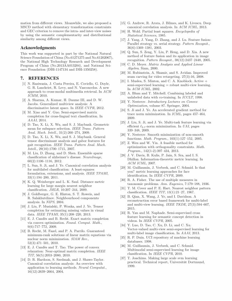
View X View Y

Multi-view

Datum

Inter-view

Noise

Mono-view

Datum

View X

Intra-view

Noise

Multi-view

Datum

Multi-view

Datum

Multi-view

Datum

Mono-view

Datum

Mono-view

Datum

Mono-view

Datum

Correlation

Correlation

Correlation

Correlation

Figure 1: Intra-View Noise and Inter-View Noise.

1. INTRODUCTIONWith the rapid development of modern information tech-

nology, a large number of high-tech digital products appearin real world. The multi-view data produced by these elec-tronic equipments become available in various fields, includ-ing medical diagnosis, webpage classification, and multime-dia analysis. These multi-view data show heterogeneouscharacteristics of low-level features and the correlation ofhigh-level semantics.

Generally, due to inappropriate data processing, man-made mistakes, random events, and the like, not all instancesare a prefect reflection of objective reality, resulting in thecorrupted views of multi-view data. Rather, the corruptedview problem in multi-view learning is essentially differentfrom single-view one. The reason is that multi-view dataare always corrupted by two different types of noise. Onerefers to the intra-view noise that makes the instances fromdifferent categories in the same view grouped together whilekeeping the samples of the same class away from each oth-er simultaneously. The other represents the noise existingamong different views, i.e., the inter-view noise, leading tofalse complementary relationship among the heterogeneousrepresentations of the same object. For example, as shown inFig.1, the existence of intra-view noise causes the zebra pho-to is incorrectly grouped with the tiger images; additionally,the unmatched white tiger picture is wrongly correlated withthe Siberian tiger image from man-made mistakes, leadingto intra-view noise.

More notably, these noise levels are high enough to affectthe performance of multi-view data, leading to false classi-fication, clustering, retrieval and analysis. Thus before ex-tracting vital information from multi-view data or next levelof processing, it is essential to denoise them to improve thequality of multi-view data for a more accurate and rigorousassessment [1, 2, 3, 4, 5]. Furthermore, to the best of our k-

∗

Zebra

Tiger

Feature 1Feature 2

Feature 3

Feature 4

Feature 1

Feature 2

Feature 3

Feature 4

Feature 5

Zebra

View X View Y

Tiger

Semantic Complementarity

Distributional Similarity

Figure 2: Complementarity and Distributivity Re-

straints on Multi-View Data.

nowledge, no existing efforts have focused on denoising thecorrupted views of multi-view data. Consequently, the above-mentioned applications face great challenge in the real world.Thus, it is necessary to develop an effective denoising methodfor multi-view corrupted data.

However, it is a challenging task to denoise the corruptedviews of multi-view data. First of all, since different viewsspan heterogeneous low-level feature spaces, there is no ex-plicit correspondence among the heterogeneous representa-tions from different views. For example, in the Alzheimer’sDisease Neuroimaging Initiative (ADNI) [6] database, ob-jects not only have Positron Emission Tomography (PET)scan, but also own Magnetic Resonance Imaging (MRI) mea-surement. Therefore, to denoise the corrupted views ofmulti-view data, an issue to be first addressed is to learna couple of heterogeneous metrics through multi-view un-corrupted data to capture the semantic complementarity a-mong different views.

Meanwhile, for multi-view data, it can be assumed as illus-trated in Fig. 2 that they are under both complementarityand distributivity constraints. The complementarity con-straint refers to the semantic complementarity among differ-ent views that makes much more the complementary infor-mation from different views fully contained in the multi-viewdata. Unlike the complementarity constraint, the distribu-tivity constraint takes high distributional similarity whichcan group the samples of the same class from the same viewtogether. Hence, another issue we need further to deal withfor denoising corrupted views is to refine multi-view corrupt-ed data under both the complementarity and distributivityconstraints.

1.1 Main ContributionsThe key contributions of this paper are highlighted as fol-

lows:

• A general framework for denoising the corrupted viewsof multi-view data is proposed to obtain the complexrepresentations for multi-view data. In this frame-work, multiple heterogeneous linear metrics are learnedto build a bridge between multiple heterogeneous low-level feature spaces.

• We propose a novel Heterogeneous Linear Metric Learn-ing (HLML) model, which linearly maps multiple het-erogeneous low-level feature spaces to a high-dimensionalfeature-homogeneous one, to capture the semantic com-plementarity and distributional similarity among dif-

ferent views. To the best of our knowledge, no otherexisting efforts have focused on this type of mapping.

• A new Multi-view Semi-supervised Collaborative De-noising (MSCD) method with elementary transforma-tion constraints and Gradient Energy Competition (GEC)criterion is proposed to remove the intra- and inter-view noise. It is worth to note that no similar methodhas been proposed in the past.

1.2 OrganizationThe remainder of this paper is organized as follows: We

present a general framework for denoising the corruptedviews of multi-view data in Section 2.1. In Section 2.2, anovel Heterogeneous Linear Metric Learning (HLML) mod-el is developed for correlating different views. We builda new Multi-view Semi-supervised Collaborative Denoising(MSCD) method to remove the intra- and inter-view noisesunder both complementarity and distributivity constraintsin Section 2.3. Furthermore, Section 3 provides two efficien-t algorithms to solve the proposed framework. Section 4gives a broad overview of some related works. Experimentalresults and analyses are reported in Section 5. Section 6concludes this paper.

1.3 NotationsWe establish some notations to be used throughout this

paper in Table 1.

Table 1: Notations

Notation Description

Vx View XVy View Y

XU ∈ Rn1×dx Uncorrupted samples in Vx

YU ∈ Rn1×dy Uncorrupted samples in Vy

LU ∈ Rn1×m Label indicator matrix

xi ∈ Rdx The i-th sample from Vx

yi ∈ Rdy The i-th sample from Vy

n1 Number of uncorrupted instancesdx Dimensionality of Vx

dy Dimensionality of Vy

m Number of labels(xi, yi) The i-th multi-view datum

XC ∈ Rn2×dx Corrupted representations in Vx

YC ∈ Rn2×dy Corrupted representations in Vy

n2 Number of corrupted instances|| · ||F Frobenius norm|| · ||

∗Trace norm

〈·, ·〉 Inner product of matrices

Sk×k+ Positive semi-definite matrices

f(·) Gradient of smooth function f(·)| · | Absolute value

Ik ∈ Rk×k Identity matrix

2. COLLABORATIVE MULTI-VIEW

DENOISINGHere we propose a general framework to denoise the cor-

rupted views of multi-view data. To facilitate the under-standing of our proposed framework, Fig. 3 gives an overallillustration of the proposed framework. More details arepresented in the following subsections.

Multi-View Heterogeneous Uncorrupted Data

x1

x2

x3

x4

x5

x6

y1

y2

y3

y4

y5

y6

XU YU

Correlation

Correlation

Correlation

Correlation

Correlation

Correlation

View X View Y

Multi-View Heterogeneous Corrupted Data

Linear

Transformation

Collaborative

Denoising

Heterogeneous Linear Metric Learning

Tiger

Zebra

Tiger

Zebra

View YView X

Metric

Metric

Metric

Metric

Metric

Metric

Heterogeneous

Complementary

x1

x2

x3

y1

y2

y3

y4

y5

y6

x6

x4

x5

y7

y8

y9

y10

x7

x8

x9

x10

XC YC

Inter-View Noise

Inter-View Noise

Inter-View Noise

Correlation

Intra-View Noise Intra-View Noise

Multi-view Semi-supervised Collaborative Denoising

View X View Y

After Denoising

x7

x8

x10

x9

y9

y8

y7

y10

Before Denoising

High-dimensional Feature-homogeneous Space

y9

y7

x7

x8

x9

y8x10

y10

Pu

sh

Switch

Switch

Figure 3: The proposed framework for collaborative multi-view denoising.

2.1 Overview of the Proposed FrameworkWe provide an overview of the proposed formulations by

using the example in Fig.3. In this example, a set of multi-view data consists of View X and View Y . There are a cer-tain amount of multi-view uncorrupted data such as (x1, y1).However, some multi-view data are corrupted. For instance,the zebra representations x9 and y10 are wrongly groupedinto the tiger category, and the co-occurring heterogeneousrepresentations in the multi-view data (x7, y7), (x8, y8), and(x9, y9) have incorrect complementary relationships.

To denoise the corrupted views of multi-view data, multi-ple heterogeneous linear metrics are learned by HLMLmodelto build a high-dimensional feature-homogeneous subspaceamong multiple heterogeneous low-level feature spaces inthe proposed framework. Specifically, to fully exploit thesemantic complementarity and distributional similarity a-mong different views, multiple heterogeneous linear metricsA and B are learned using the multi-view uncorrupted da-ta XU and YU to eliminate the heterogeneity across them.Thus, a feature-homogeneous subspace is obtained, in whichthe correlated representations from different views are cou-pled together to capture much more complementary infor-mation from different views. At the same time, the samplesof the same class from the same view can be grouped to-gether while keeping the instances from different categoriesaway from each other simultaneously. For example, the ze-bra heterogeneous representations x6 and y6 are matchedtogether to capture much more complementary informationfrom different views. Furthermore, the tiger co-occurringheterogeneous representations (x1, y1), (x2, y2), and (x3, y3)and the zebra co-occurring heterogeneous representations(x4, y4), (x5, y5), and (x6, y6) are grouped together respec-

tively to mine the distributional similarity among differentviews.

Meanwhile, by exploiting multiple heterogeneous metricslearned by HLML model, the intra-view noises existing inthe multi-view corrupted data XC and YC are removed byMSCD model to a large extent in the feature-homogeneousspace on the basis of both semantic complementarity anddistributional similarity among different views. Moreover,the MSCD method utilizes the proposed elementary trans-formation constraints based on GEC criterion to establishthe complementary relationship among the heterogeneousrepresentations of the same object according to the learnedmultiple heterogeneous metrics. The constraints will switchthe positions of corresponding representations in the cor-rupted matrix XC and YC to eliminate the inter-view noises.For instance, the zebra representation x9 in the View X ispulled out the group composed of the tiger representationsx7 and x8; besides, the zebra representation y10 in the ViewY is pushed closer to the cluster consisting of the zebra rep-resentations to remove intra-view noise; and the zebra repre-sentations y7 and y9 in the View Y are switched respectivelyto match the appropriate representations to eliminate inter-view noise effectively. After denoising, the heterogeneousrepresentations from different views are correctly matchedand grouped together in the feature-homogeneous space.

2.2 The Proposed HLML ModelIn the following, a novel multi-view metric learning method

is developed for capturing both semantic complementarityand distributional similarity among different views in thissubsection. Our work is motivated by a few prior stud-ies. Recently, Sun et al [7] have proved that the homo-geneous transformations can significantly capture the com-

plementarity among different views. Moreover, Weinberg-er et al [8] have pointed out that the pseudo-metric basedon Mahalanobis distance can be used to effectively elimi-nate the intra-view noise. Furthermore, Goldberger et al[9] have proved that the Mahalnobis distance metric basedon leave-one-out validation can exploit the characteristics ofsample distribution to improve the performance of classifi-cation. Additionally, Liu et al [10] have pointed out that therank is a powerful tool to capture between-class differencesin the matrix case. Nevertheless, “rank(•)” is not a convexfunction, which leads to the difficulty in finding the optimalsolution. Fortunately, Candes and Recht [11], Recht et al[12], and Candes and Tao [13] have theoretically justifiedthat the trace norm of a matrix can be used to approximatethe rank of the matrix.

Following the above-mentioned strong theoretical support-s [7, 8, 9, 10, 11, 12, 13], we propose a novel HLML modelwith low-rank regularization, leave-one-out validation, andpseudo-metric constraints to learn multiple heterogeneouslinear transformations for multi-view data, as shown in Fig.4.Particularly, the existing uncorrupted heterogeneous repre-sentations XU and YU are utilized in HLML model to learnmultiple well-defined pseudo-metrics A and B to mine thedistributional similarity among different views. Then, tomake transformed data MU and RU maximally linearly sep-arable, it is essential to impose the low-rank regularizationon the transformed data. As a consequence, the heteroge-neous representations are linearly projected into a feature-homogeneous space, in which the correlated representationsfrom different views are coupled together to capture the se-mantic complementarity among different views.

More specifically, the new distance metrics are defined asfollows to learn a Mahalanobis distance:

DMX(xi, xj) = (xi − xj)

TMX(xi − xj), (1)

DMY(yi, yj) = (yi − yj)

TMY (yi − yj), (2)

where MX = ATA and MY = BTB are two positive semi-definite matrices. Thus, the linear transformations A andB can be applied to each pair of co-occurring heterogeneousrepresentations (xi, yi).

Assuming CtX and Ct

Y be the sample sets of t-th class fromthe views Vx and Vy , respectively. We define each sample xi

or yi selects another sample yj or xj in another view as itsneighbor with the probability pij or qij . By using a softmaxunder the Euclidean distance in the transformed feature-homogeneous space, pij and qij are defined as follows:

pij =exp(− ‖ Axi −Byj ‖2)∑k exp(− ‖ Axi −Byk ‖2)

, (3)

qij =exp(− ‖ Byi − Axj ‖2)∑k exp(− ‖ Byi − Axk ‖2)

. (4)

Under this definition, we can compute the probabilities piand qi that the sample i will be correctly classified:

pi =∑

xi∈CtX

& yj∈CtY

pij , (5)

qi =∑

yi∈CtY

& xj∈CtX

qij , (6)

Uncorrupted

Representations XU

Heterogeneous Matrix

Uncorrupted

Representations YU

Heterogeneous Matrix

Pseudometric Matrix

Linear

Transformation A

Linear

Transformation B

Class 1

Class 2

Linearly-Separable

Representations MU

Feature-Homogenous Matrix

Pseudometric Matrix

Rank

Rank

Linearly-Separable

Representations RU

Class 1

Class 2

Feature-Homogenous Matrix

Figure 4: Heterogeneous Linear Metric Learning.

Then the proposed approach can be formulated as follows:

Ψ1 :minA,B

‖ XUA− YUB ‖2F −αg(A,B) + βh(A,B)

s.t. ATA 0 and BTB 0,(7)

where A ∈ Rdx×k, B ∈ R

dy×k, k is the dimensionality ofthe feature-homogeneous subspace, the positive semidefiniteconstraints ATA 0 and BTB 0 are added into the opti-mization to ensure a well-defined pseudo-metric, and α andβ are two trade-off parameters. The first term in the ob-jective function is used to capture the semantic complemen-tarity among different views. The motivation of introducingthe leave-one-out validation g(A,B)

g(A,B) =∑

pi +∑

qi, (8)

consisting of the classification accuracies of different views isto mine the distributional similarity among different views.In addition, the third term h(A,B) in the objective function

h(A,B) =‖ XUA ‖∗ + ‖ YUB ‖∗, (9)

is a low-rank regularization based on trace norm to maketransformed data MU and RU carrying more between-classdifferences information.

It is worth to note that no similar numerical method hasbeen yet proposed. Our proposed HLML model is greatly d-ifferent from well-known kernel methods [14, 15] without anexplicit high-dimensional projection and classical linear al-gorithms [7, 16] to reduce dimensionality. HLML can linear-ly project the multi-view data into a feature-homogeneousspace of even higher dimensions. That is to say, k may begreater than both dx and dy, i.e., k ≥ max(dx, dy).

Furthermore, the Parallel Feature Fusion Strategy (PFFS)[17, 18] is adopted to establish the common representations.The details is as follows: for the i-th pair of heterogeneousrepresentations (xi, yi), we can obtain their own Homoge-neous Correlated Representations (HCR) with the optimalA∗ and B∗ by:

µxi= A∗Txi and µyi = B∗T yi. (10)

Consequently, we can obtain a Complex Representations(CR) µi in the feature-homogeneous subspace based on µxi

and µyi :

µi = (µxi+ µyi)/2. (11)

In Section 3.1, an efficient algorithm is proposed to solvethe problem Ψ1.

Figure 5: Multi-view Semi-supervised Collaborative

Denoising.

2.3 The Proposed MSCD ModelIn the above subsection, we have built a high-dimensional

feature-homogeneous space by multiple learned heteroge-neous linear metrics to capture both semantic complemen-tarity and distributional similarity among different views.Furthermore, to eliminate the intra- and inter-view noise,it is essential to recover the complementary relationship a-mong the heterogeneous representations of the same objectin the multi-view corrupted data on the basis of the learnedheterogeneous metrics.

In [19], it has been pointed out that an elementary rowtransformation matrix can be used to exchange any rows ofa matrix. Additionally, Rubinstein et al [20] have proposedrecently a forward-looking energy function that measuresthe effect of seam carving on the retargeted image, not theoriginal one. They have shown how the new measure canbe used in either graph cut or dynamic programming anddemonstrated the effectiveness of their contributions on sev-eral images and video sequences. Moreover, it has been tes-tified in [21] by Muslea et al that the robust performanceof multi-view learning depends on interleaving active andsemi-supervised learning on the basis of view correlation.Furthermore, Blum and Mitchell [22] have proved that for aproblem with two views the target concept can be learnedbased on a few labeled and many unlabeled examples, pro-vided that the views are compatible and heterogeneous.

Based on the above-mentioned strong theoretical supports[19, 20, 21, 22], we propose a new MSCD model with elemen-tary transformation constraints and GEC criterion to elimi-nate the intra- and inter-view noises according to the learnedsemantic complementarity and distributional similarity a-mong different views in Section 2.2. As shown in Fig.5,MSCD model eliminates the intra- and inter-view noises bymeans of semi-supervised learning. It firstly makes use ofthe uncorrupted linearly-separable representations MU andRU with labels to learn a decision matrix W . Then throughthe learned elementary row transformation matrices T andH , MSCD switches the positions of the noise-corrupted sam-ples in the matrices MC and RC ; meanwhile, the decisionmatrix W is applied to predict the classification of the un-labeled noisy representations MC and RC to establish thecomplementary relationship among the heterogeneous rep-resentations of the same object.

Specifically, let (A∗, B∗) be the optimal solutions of the

problem Ψ1. Then the proposed approach can be formulatedas follows:

Ω1 :

minT,H,W

‖ TMCW −HRCW ‖2F +

γ ‖

[MU

RU

]W −

[LU

LU

]‖2F +τ ‖ W ‖2F

s.t. T,H ∈ En2and W TW =I,

(12)

where T∈Rn2×n2 and H∈Rn2×n2 are two elementary rowtransformation matrices, W ∈ R

k×m is a decision matrix,MC = XCA

∗ and RC = YCB∗ are the noise-corrupted ma-

trices in ViewX and View Y , respectively, MU = XUA∗ and

RU = YUB∗ are the uncorrupted linearly-separable repre-

sentations in the feature-homogeneous space, En2∈ R

n2×n2

is a set of elementary row transformation matrices, and γand τ are two regularization parameters. The first term inthe objective function takes advantage of the learned W ,T , and H to recover the complementary relationship amongthe heterogeneous representations of the same object. Thesecond term in the objective function is a linear least squareloss to learn an excellent decision matrix W using the uncor-rupted linearly-separable representations MU and RU withlabels. The goal of imposing the orthogonal constraints onW is to effectively remove the correlations among differ-ent classes. The motivation of introducing the elementarytransformation constraints is to ensure the matrices T andH be two standard elementary row transformation matricesto switch the positions of the noise-corrupted samples in thematrices MC and RC .

Recently, the gradient energy measure has been widelyused in dynamic programming and demonstrated its effec-tiveness on graph cut or seam carving[20]. Based on theabove strong theoretical supports, we propose a GradientEnergy Competition (GEC) criterion to build an elemen-tary row transformation matrix.

In detail, in a gradient matrix G obtained by gradient de-scent method, every internal element Gij is connected to itsfour neighbors Gi−1,j , Gi+1,j , Gi,j−1, and Gi,j+1. Followingthe ℓ1-norm gradient magnitude energy [20], we define thebetween-sample energy Ebs of Gij in the vertical directionas

Ebs =∂

∂xG =| G(i+ 1, j)−G(i, j) | +

| G(i, j)−G(i− 1, j) |,(13)

and the within-sample energy Ews in the horizontal directionas

Ews =∂

∂yG =| G(i, j + 1)−G(i, j) | +

| G(i, j) −G(i, j − 1) | .(14)

The global energy of Gij can be obtained via Ebs and Ews:

Eglobe = δ ∗ Ebs + (1− δ) ∗ Ews, (15)

where δ is a trade-off parameter. We use Eq.(15) to compute

Gradient Matrix G

Between-Sample

Energy Ebs

Within-Sample

Energy Ews

Gi-1,j

Gi,j-1 Gi,j Gi,j+1

Gi+1,j

Competition Circulation

Energy Matrix E

Winner

Row Transformation T

Elementary Matrix

Figure 6: Gradient Energy Competition.

Algorithm 1: Heterogeneous Linear Metric Learning (HLML)

Input: F (·), D(·), h(·), Z0=[AZ0BZ0

], β, XU , YU ,γ1 > 0, t0=1, and max−iter.

Output: Z∗.1: Define Fγ,S(Z)=D(S)+〈D(S), Z−S〉+γ‖Z−S‖2F /2+

βh(Z)2: Set AZ1

= AZ0and BZ1

= BZ0.

3: for i =1,2,· · ·,max−iter do4: Set ai = (ti−1 − 1)/ti−1.5: Compute ASi

= (1 + αi)AZi− αiAZi−1

.6: Compute BSi

= (1 + αi)BZi− αiBZi−1

.7: Set Si = [ASi

BSi].

8: Compute ASD(ASi

) and BSD(BSi

).9: while (true)

10: Compute AS = ASi− AS

D(ASi)/γi.

11: Compute [AZi+1] = PSP(AS).

12: Compute BS = BSi− BS

D(BSi)/γi.

13: Compute [BZi+1] = PSP(BS).

14: Set Zi+1 = [AZi+1BZi+1

].15: if F (Zi+1) ≤ Fγi,Si

(Zi+1), then break;16: else Update γi = γi × 2.17: end-if18: end-while

19: Update ti =(1+

√1+4t2i−1

)/2, γi+1=γi.

20: end-for21: Set Z∗ = Zi+1.

global energy of every element in the matrix G, and then anenergy matrix E can be obtained. Furthermore, the globalenergies of every element in the matrix E are compared. Asshown in Fig.6, the winner which owns the greatest energywill be set to 1, the rest of the elements in the same rowand column to 0. And the cycle repeats until a standardelementary transformation matrix T is established. It isworth to note that no similar method has been yet proposed.

Section 3.2 presents an efficient algorithm to compute theoptimum for the problem Ω1.

3. EFFICIENT ALGORITHMS FOR THE

PROPOSED FRAMEWORKHere we provide two efficient algorithms to solve the pro-

posed framework. Specifically, an iterative algorithm forsolving the HLML model Ψ1 (see Section 2.2) is presentedin the Section 3.1. Moreover, the Section 3.2 shows how tosolve the MSCD model Ω1 proposed in Section 2.3.

3.1 An Efficient Solver for Ψ1

For notational simplicity, we denote the optimization prob-lem Ψ1 in Eq.(7) by:

minZ∈C

F (Z) = D(Z) + βh(Z), (16)

where D(·) = ‖ · ‖2F − αg(·) is a smooth objective function,Z=[AZ BZ ] symbolically represents the optimization vari-ables, and C is the closed and separately convex domain withrespect to each variable:

C = Z|ATZAZ 0, BT

ZBZ 0. (17)

As D(·) is continuously differentiable with Lipschitz contin-

uous gradient L [23]:

‖D(Zx)−D(Zy)‖F ≤ L‖Zx−Zy‖F ,∀Zx, Zy ∈C, (18)

thus it is appropriate to adopt the Accelerated ProjectedGradient (APG) [23, 24, 25] method to solve Eq.(16).

The APG algorithm is a first-order gradient method, whichcan accelerate each gradient step on the feasible solutionto obtain an optimal solution when minimizing a smoothfunction [26]. This method will construct a solution pointsequence Zi and a searching point sequence Si, whereeach Zi is updated from Si.

Note that, in the APG algorithm, the Euclidean projec-tion of a given point s onto the convex set C can be definedby:

projC(s) = arg minz∈C

‖z − s‖2F /2. (19)

Weinberger et al. proposed a Positive Semi-definite Projec-tion (PSP) [8] to minimize a smooth function while remain-ing positive semi-definite constraints. Then we can use thePSP to solve the problem in Eq.(19).

Finally, when applying the APG method for solving theproblem in Eq.(16), the projection Z = [AZ BZ ] of a givenpoint S = [AS BS ] onto the set C is defined by:

projC(S) = arg minZ∈C

‖Z − S‖2F /2. (20)

By combining APG and PSP, we can solve the problem inEq.(20). The details are given in Algorithm 1.

Algorithm 2: Energy

Input: G ∈ Rn, δ.

Output: an energy matrix E ∈ Rn.

1: for i =1,2,· · ·,n do2: for j =1,2,· · ·,n do3: if i−1≤0 && i+1≤n && j−1≤0 && j+1≤n4: Ebs = |Gi+1,j −Gi,j |, Ews = |Gi,j+1 −Gi,j |.5: elseif i−1≤0 && i+1≤n && j−1>0 && j+1≤n6: Ebs = |Gi+1,j −Gi,j |.7: Ews = |Gi,j+1 −Gi,j |+ |Gi,j −Gi,j−1|.8: elseif i−1≤0 && i+1≤n && j−1>0 && j+1>n9: Ebs = |Gi+1,j −Gi,j |, Ews = |Gi,j −Gi,j−1|.10: elseif i−1>0 && i+1≤n && j−1≤0 && j+1≤n11: Ebs = |Gi+1,j −Gi,j |+ |Gi,j −Gi−1,j |.12: Ews = |Gi,j+1 −Gi,j |.13: elseif i−1>0 && i+1≤n && j−1>0 && j+1≤n14: Ebs = |Gi+1,j −Gi,j |+ |Gi,j −Gi−1,j |.15: Ews = |Gi,j+1 −Gi,j |+ |Gi,j −Gi,j−1|.16: elseif i−1>0 && i+1≤n && j−1>0 && j+1>n17: Ebs = |Gi+1,j −Gi,j |+ |Gi,j −Gi−1,j |.18: Ews = |Gi,j+1 −Gi,j |.19: elseif i−1>0 && i+1>n && j−1≤0 && j+1≤n20: Ebs = |Gi,j −Gi−1,j |, Ews = |Gi,j+1 −Gi,j |.21: elseif i−1>0 && i+1>n && j−1>0 && j+1≤n22: Ebs = |Gi,j −Gi−1,j |.23: Ews = |Gi,j+1 −Gi,j |+ |Gi,j −Gi,j−1|.24: elseif i−1>0 && i+1>n && j−1>0 && j+1>n25: Ebs = |Gi,j −Gi−1,j |, Ews = |Gi,j −Gi,j−1|.26: end-if27: Compute Eij = δ ∗Ebs + (1− δ) ∗Ews.28: end-for29: end-for

3.2 An Efficient Solver for Ω1

This subsection provides an efficient algorithm to solvethe model Ω1 proposed in Section 2.3. Similarly, the opti-mization problem Ω1 can be simplified as:

minZ∈Q

Q(Z), (21)

where Q(·) = ‖ · ‖2F is a smooth objective function, Z =[TZ HZ WZ ] symbolically represents the optimization vari-ables, and Q is the closed domain set with respect to eachvariable:

Q = Z|TZ ∈ En2,HZ ∈ En2

, and W TZ WZ = I. (22)

Similarly, as Q(·) is continuously differentiable with Lips-chitz continuous gradient L [23] in the Eq.(18), it is alsoappropriate to adopt the Accelerated Projected Gradient(APG) [23] method to solve the problem in Eq.(21).

In like manner, we can define the Euclidean projection ofa given point s onto the closed set Q in the APG algorithmas:

projQ(s) = arg minz∈Q

‖z − s‖2F /2, (23)

To solve the Eq.(23), we use the proposed GEC criterion inSection 2.3 to project the approximate solution of the prob-lem into the elementary transformation constraint Q. Twonew functions Energy(·) and Competition(·) are designedin this subsection to implement the GEC criterion.

The proposed function Energy(·) in Algorithm 2 will com-pute the global energy of every internal element in the gra-dient matrix G obtained by gradient descent method onthe basis of the position of each element according to E-q.(13,14,15). Thus, an energy matrix E can be obtained.

In addition, we also develop a Competition(·) function inAlgorithm 3 to establish a standard elementary transforma-tion matrix according to the energy matrix E produced byAlgorithm 2.

Algorithm 3: Competition

Input: E ∈ Rn.

Output: Z ∈ Rn.

1: Build a zero matrix Z ∈ Rn.

2: for i =1,2,· · ·,n do3: Find the row and column coordinates r and c of

the maximum value of the matrix E.4: Set Zr,c = 1.5: Replace the other components of r-th row and

c-th column in the matrix E with 0.6: end-for

Note that the orthogonality constraints are included in E-q.(21). Recently, the Gradient Descent Method with Curvi-linear Search (GDMCS) [27] proposed by Wen and Yin caneffectively deal with these difficulties. Thus, we can use theGDMCS to preserve the orthogonality of a given point s inEq.(21). By combining APG, Algorithm 2 and 3, and GDM-CS, we can solve the problem in Eq.(21). The details aregiven in Algorithm 4, where the function Schmidt(·) [19]denotes the GramSchmidt process.

4. RELATED WORKThis section reviews some related works. We begin by

discussing some prior methods for mining the correlationbetween different views in multi-view learning. And then s-

Algorithm 4: Multi-view Semi-supervised CollaborativeDenoising (MSCD)

Input: Q(·), TZ0=In, HZ0

=In, WZ0, Z0=[TZ0

HZ0WZ0

],δ, γ1 > 0, t0=1, τ1, 0 < ρ = [ρ1 ρ2] < 1, and max−iter.Output: Z∗.1: Define Qγ,S(Z)=Q(S)+〈Q(S),Z−S〉+γ‖Z−S‖2F /2.2: Compute [WZ0

] = Schmidt(WZ0).

3: Set TZ1= TZ0

, HZ1= HZ0

, and WZ1= WZ0

.4: for i =1,2,· · ·,max−iter do5: Set ai = (ti−1 − 1)/ti−1.6: Compute TSi

= (1 + αi)TZi− αiTZi−1

.7: Compute HSi

= (1 + αi)HZi− αiHZi−1

.8: Compute WSi

= (1 + αi)WZi− αiWZi−1

.9: Set Si = [TSi

HSiWSi

].10: Derive TS

Q(TSi),HS

Q(HSi), andWS

Q(WSi).

11: while (true)

12: Compute TS = −TSQ(TSi

)/γi.

13: Compute [TZi+1] = Energy(TS , δ).

14: Compute [TZi+1] = Competition(TZi+1

).

15: Compute HS = −HSQ(HSi

)/γi.

16: Compute [HZi+1] = Energy(HS).

17: Compute [HZi+1] = Competition(HZi+1

).

18: Compute WS = WSi− WS

Q(WSi)/γi.

19: Compute [WZi+1] = Schmidt(WS).

20: Compute [WZi+1] = GDMCS(WZi+1

, τ1, ρ).21: Set Zi+1 = [TZi+1

HZi+1WZi+1

].22: if Q(Zi+1) ≤ Qγi,Si

(Zi+1), then break;23: else Update γi = γi × 2.24: end-if25: end-while

26: Update ti =(1+

√1+4t2i−1

)/2, γi+1=γi.

27: end-for28: Set Z∗ = Zi+1.

ome representative linear metric learning technologies formono-view data are investigated to show the correlation be-tween them and our proposed work. Finally, some multi-view semi-supervised learning algorithms to bootstrap clas-sifiers in each view are studied.

4.1 Feature Homogeneous MethodsTo eliminate the heterogeneity across different views, many

feature homogeneous techniques based on Subspace Learn-ing (SL) [7, 16, 14, 15] have been proposed recently.

CCA (Canonical Correlation Analysis) [7] and PLS (Par-tial Least Squares) [16] are two classical statistical analysistechniques for modeling correlation between sets of observedvariables. They both compute low-dimensional embeddingof sets of variables simultaneously. The main difference ofthem is that CCA maximizes the correlation between vari-ables in the embedded space, while PLS maximizes theircovariance. Kernel CCA (KCCA) [14] offers a nonlinearalternative solution for CCA by implicitly mapping multi-view data into a high-dimensional feature-homogeneous s-pace. Unlike KCCA, Deep CCA (DCCA) in [15] does notrequire an inner product, which provides a flexible nonlinearalternative to KCCA.

4.2 Linear Metric LearningMany representative metric learning algorithms, such as

Large Margin Nearest Neighbors (LMNN) [8], InformationTheoretic Metric Learning (ITML) [28], Neighborhood Com-ponent Analysis (NCA) [9], Logistic Discriminative MetricLearning (LDML) [29], and Linear Discriminant Analysis(LDA) [30], are based on linear transformation and distancemetric.

Weinberger et al. [8] proposed a linear metric learning al-gorithm called LMNN based Mahalanobis distance [8] for k-Nearest Neighbors (kNN) [31] classification. ITML [28] usesa one to one correspondence between the Mahalanobis dis-tance to minimize the differential relative entropy betweentwo multivariate Gaussians under constraints on a distancefunction. NCA [9] is another linear metric learning methodto find a distance metric that maximizes the performanceof kNN classification, measured by Leave-One-Out (LOO)validation. A logistic discriminant approach based marginalprobability named LDML was presented by Guillaumin etal. [29] to learn a metric from a set of labelled image pairs.LDA [30] is widely used as a form of linear preprocessingfor pattern classification, which is operated in a supervisedsetting and uses the class labels of the inputs to derive in-formative linear projections.

4.3 Multi-View Semi-Supervised LearningRecently, some researchers have investigated many semi-

supervised learning methods [21, 32, 33, 34] to deal withvarious multi-view problems.

Muslea et al. pointed out in [21] that the robustnessof multi-view learning came from the combination of semi-supervised and active learning. In [32], Qian et al. presenteda joint learning framework based on reconstruction error,namely Semi-Supervised Dimension Reduction for Multi-label and Multi-view Learning (SSDR-MML), to performoptimization for dimension reduction and label inferencein multi-label and multi-view learning settings. Yan andNaphade [33] proposed a novel multi-view semi-supervisedlearning algorithm called Semi-supervised Cross Feature Learn-ing (SCFL) for detecting the video semantic concepts, whichcan handle additional views of unlabeled data even whenthese views were absent from the training data. A Multi-View Vector-Valued Manifold Regularization (MV3MR) al-gorithm was developed in [34] to integrate multiple featuresfrom different views in the learning process of the vector-valued function.

5. EXPERIMENTAL EVALUATIONIn this section, we evaluate and analyze the effectiveness

of the proposed formulations and algorithms for denoisingthe corrupted views of multi-view data.

5.1 DatasetsOur experiments are conducted on three publicly available

multi-view datasets, namely, UCI Multiple Features (UCIMFeat) [35], COREL 5K [36], and Alzheimer’s Disease Neu-roimaging Initiative (ADNI) [6].

5.2 Experimental SetupNote that all the data are normalized to unit length. Each

dataset is randomly separated into a training set and a testset. The training samples account for 80 percent of eachoriginal dataset, and the remaining ones act as the test data.Such a partition of each dataset is repeated five times andthe average performance is reported. In the training and

test sets, 10 percent of multi-view data have corrupted view(We rearrange the corresponding relationships among thesemulti-view data in random order, and corrupt them by whiteGaussian noise.).

Some key parameters of all the methods in our experi-ments are tuned using the 5-fold cross-validation based onthe AUC (area under the receiver operating characteristiccurve) on the training set. Particularly, the LIBSVM clas-sifier serves as the benchmark for the tasks of classificationin the experiments.

5.3 Comparison of Feature Homogeneous Al-gorithms

Since the proposed HLML model and other classical fea-ture homogeneous methods such as CCA [7], PLS [16], KC-CA [14], and DCCA [15] are based on subspace learning,we compare their classification performance to show the im-portance of mining the distributional similarity among d-ifferent views. Here, the dimensionality k of the feature-homogeneous space is specified by min(dx, dy) for CCA andPLS. For KCCA and DCCA, we tune the dimensionalityk on the candidate set i × 200|i = 1, 2, 3, · · · , 10, andGaussian kernel is used in KCCA. The dimensionality k ofthe feature-homogeneous subspace is set to max(dx, dy) inHLML, and the trade-off parameters α and β are tuned onthe sets 10i|i = −2,−1, 0, 1, 2..

Due to their inherent limitations, PLS and CCA can on-ly project the multi-view data into a low-dimensional spaceaccording to Eq.(11) without the full consideration of dis-tributional similarity among different views. Therefore, thefeature-homogeneous spaces learned by PLS and CCA maycontain much more noise, which groups the instances fromdifferent categories together while keeping the samples ofthe same class away from each other simultaneously. Ad-ditionally, KCCA and DCCA offer an alternative solutionby nonlinearly mapping the multi-view data into a feature-homogeneous space. However, it is very difficult for KCCAand DCCA to capture much distributional information with-out leave-one-out validation and low-rank regularization.

Table 2: Classification Performance of Feature Ho-

mogeneous Methods in terms of AUC

MethodDataset

UCI MFeat COREL 5K ADNI

CCA 0.7936 0.5376 0.7519PLS 0.8016 0.5597 0.7846

KCCA 0.6371 0.5738 0.8096DCCA 0.8494 0.5393 0.8196HLML 0.9536 0.7213 0.8339

The proposed HLML model linearly maps multiple het-erogeneous low-level feature spaces to a high-dimensionalfeature-homogeneous one using pseudo-metric constraints.As shown in Table 2, the superiority of HLML over CCA,PLS, KCCA, and DCCA in the classification performance isquite clear. For example, nearly 20 percent gain is achievedfor the COREL 5K dataset. It means that HLML can learnthe distributional similarity among different views more ef-fectively than CCA, PLS, KCCA, and DCCA.

Number of samples

20% 40% 60% 80% 100%0.5

0.55

0.6

0.65

0.7

0.75HLML LMNN ITML NCA LDA

Figure 7: Comparisons of Classification Perfor-

mance of Metric Learning Methods.

5.4 Analysis of Metric Learning MethodsTo validate the heterogeneous metrics learned by the pro-

posed HLML method, we analyze HLML on the task of clas-sification with other four representative and state-of-the-artmetric learning methods such as LMNN [8], ITML [28], N-CA [9], and LDA [30]. This experiment is conducted in thelarger COREL 5K dataset. We randomly sample data inthe ratio 20%, 40%, 60%, 80%, 100% from the training setas the training instances and fix the testing set. For LMNN,ITML, NCA, and LDA, the experiment settings follow theoriginal works [8, 28, 9, 30], respectively. ITML uses iden-tity matrix as initial metric matrix. Moreover, we used thecodes provided by the authors for LMNN, ITML, and NCA.

Similar to LMNN and ITML, the proposed HLML mod-el is also a metric method based on Mahalanobis distance.But the major difference of HLML with the other model-s lies in that it fully takes into account the distributionalsimilarity among different views. In addition, though NCAalso use leave-one-out validation to exploit the characteris-tics of sample distribution, the correlation among hetero-geneous representations in multi-view data is not utilizedfully. Moreover, since LDA is originally developed for han-dling mono-view problem, it can only learn some limiteddistributional information among different views.

We can see from Fig.7 that HLML is superior to othermetric learning methods in classification performance. Thisobservation further confirms that HLML can effectively cap-ture both semantic complementarity and distributional simi-larity among different views. Furthermore, with the increas-ing of training sample, the performance of HLML will im-prove. Thus, HLML also has some limitations that it need acertain number of existing samples to learn a set of excellentmetrics.

5.5 Comparison of Multi-View Semi-SupervisedLearning

In essence, like SSDR-MML [32], SCFL [33], and MV3MR[34], the proposed MSCD model is also a multi-view semi-supervised learning method using both labeled and unla-beled data simultaneously. But the explicit difference ofMSCD from the former models lies in that it fully takes in-to account the semantic complementarity among differentviews. So the latter will be more favorable to reduce intre-view noise for reestablishing the complementary relationshipamong heterogeneous representations.

To validate this point, we first use HLML to project the

multi-view data into a feature-homogeneous space and thenapply SSDR-MML, SCFL, MV3MR, and MSCD to denoisecorrupted view. The performances of the classifiers learnedby MSCD and other methods are compared in three multi-view dataset. For MSCD, the elementary row transforma-tion matrices T and H are set to identity matrices. We tunethe regularization parameters γ and τ on the set 10i| =−2,−1, 0, 1, 2. The parameter δ in GEC criterion (see E-q.(15)) is specified by 0.1. The decision matrix W ∈Rk×m

is randomly initialized. The regularization parameter λ inSSDR-MML is set to 1, and following the original work [32],the maximization of learning success measure is adopted todetermine the importance of each label. For SCFL [33],SVMLight [37] serves as the underlying classifier where thelinear kernel is applied for View Vx and the RBF kernel forView Vy. The parameter setting in MV3MR is the same asin its original reference [34]. Additionally, we also comparethe classification performances of the methods in each itera-tion round in COREL 5K dataset to verify the convergenceof the proposed MSCD algorithm.

Table 3: Classification Performance of SSDR-MML,

SCFL, MV3MR and MSCD in terms of AUC

MethodDataset

UCI MFeat COREL 5K ADNI

SSDR-MML 0.7371 0.6738 0.8039SCFL 0.8494 0.6393 0.8172

MV3MR 0.7826 0.6857 0.8169MSCD 0.9149 0.7087 0.8219

As shown in Table 3, the superiority of MSCD over SSDR-MML, SCFL, and MV3MR in the classification performanceis quite clear. This result shows that, in contrast to thecompared approaches, MSCD is effective on reducing intre-view noise. Moreover, it can be observed from Fig.8 thatMSCD shows an obvious advantage over the other methodsin every iteration and converges as well. This observationindicates that the MSCD is superior to other multi-viewsemi-supervised learning methods in rebuilding the semanticcomplementarity among different views.

6. CONCLUSIONIn this paper, we have investigated the corrupted views

problem in multi-view learning. We developed a gener-al framework to denoise corrupted views to obtain CR formulti-view data. Within this framework, multiple hetero-geneous linear metrics are learned by the proposed HLMLmodel with pseudo-metric constraints, leave-one-out valida-tion, and low-rank regularization to unfold the shared infor-

Number of iteration

0 50 100 150 200

AU

C

0.50

0.55

0.60

0.65

0.70

0.75SSDR-MML SCFL MV3MR MSCD

Figure 8: Comparison in each iteration round.

mation from different views. Meanwhile, we also proposed aMSCD method with elementary transformation constraintsand GEC criterion to remove the intra- and inter-view noisesby using the semantic complementarity and distributionalsimilarity among different views.

Acknowledgments

This work was supported in part by the National NaturalScience Foundation of China (No.61271275 and No.61202067),the National High Technology Research and DevelopmentProgram of China (No.2013AA013204), and National Sci-ence Foundation (DBI-1147134 and DBI-1350258).

7. REFERENCES[1] N. Rasiwasia, J. Costa Pereira, E. Coviello, G. Doyle,

G. R. Lanckriet, R. Levy, and N. Vasconcelos. A newapproach to cross-modal multimedia retrieval. In ACM

ICMM, 2010.

[2] A. Sharma, A. Kumar, H. Daume III, and D. W.Jacobs. Generalized multiview analysis: Adiscriminative latent space. In IEEE CVPR, 2012.

[3] M. Xiao and Y. Guo. Semi-supervised matrixcompletion for cross-lingual text classification. InAAAI, 2014.

[4] D. Tao, X. Li, X. Wu, and S. J. Maybank. Geometricmean for subspace selection. IEEE Trans. Pattern

Anal. Mach. Intell., 31(2):260–274, 2009.

[5] D. Tao, X. Li, X. Wu, and S. J. Maybank. Generaltensor discriminant analysis and gabor features forgait recognition. IEEE Trans. Pattern Anal. Mach.

Intell., 29(10):1700–1715, 2007.

[6] M. Liu, D. Zhang, and D. Shen. Ensemble sparseclassification of alzheimer’s disease. NeuroImage,60(2):1106–1116, 2012.

[7] L. Sun, S. Ji, and J. Ye. Canonical correlation analysisfor multilabel classification: A least-squaresformulation, extensions, and analysis. IEEE TPAMI,33(1):194–200, 2011.

[8] K. Q. Weinberger and L. K. Saul. Distance metriclearning for large margin nearest neighborclassification. JMLR, 10:207–244, 2009.

[9] J. Goldberger, G. E. Hinton, S. T. Roweis, andR. Salakhutdinov. Neighbourhood componentsanalysis. In NIPS, 2004.

[10] J. Liu, P. Musialski, P. Wonka, and J. Ye. Tensorcompletion for estimating missing values in visualdata. IEEE TPAMI, 35(1):208–220, 2013.

[11] E. J. Candes and B. Recht. Exact matrix completionvia convex optimization. Found. Comput. Math.,9(6):717–772, 2009.

[12] B. Recht, M. Fazel, and P. A. Parrilo. Guaranteedminimum-rank solutions of linear matrix equations vianuclear norm minimization. SIAM Rev.,52(3):471–501, 2010.

[13] E. J. Candes and T. Tao. The power of convexrelaxation: Near-optimal matrix completion. IEEETIT, 56(5):2053–2080, 2010.

[14] D. R. Hardoon, S. Szedmak, and J. Shawe-Taylor.Canonical correlation analysis: An overview withapplication to learning methods. Neural Computat.,16(12):2639–2664, 2004.

[15] G. Andrew, R. Arora, J. Bilmes, and K. Livescu. Deepcanonical correlation analysis. In ACM ICML, 2013.

[16] H. Wold. Partial least squares. Encyclopedia of

Statistical Sciences, 1985.

[17] J. Yang, J. Yang, D. Zhang, and J. Lu. Feature fusion:Parallel strategy vs. serial strategy. Pattern Recognit.,36(6):1369–1381, 2003.

[18] Q. Sun, S. Zeng, Y. Liu, P. Heng, and D. Xia. A newmethod of feature fusion and its application in imagerecognition. Pattern Recognit., 38(12):2437–2448, 2005.

[19] C. D. Meyer. Matrix Analysis and Applied Linear

Algebra. Siam, 2000.

[20] M. Rubinstein, A. Shamir, and S. Avidan. Improvedseam carving for video retargeting. 27(3):16, 2008.

[21] I. Muslea, S. Minton, and C. A. Knoblock. Active +semi-supervised learning = robust multi-view learning.In ACM ICML, 2002.

[22] A. Blum and T. Mitchell. Combining labeled andunlabeled data with co-training. In ICCLT, 1998.

[23] Y. Nesterov. Introductory Lectures on Convex

Optimization, volume 87. Springer, 2004.

[24] S. Ji and J. Ye. An accelerated gradient method fortrace norm minimization. In ICML, pages 457–464,2009.

[25] J. Liu, S. Ji, and J. Ye. Multi-task feature learning viaefficient ℓ2,1-norm minimization. In UAI, pages339–348, 2009.

[26] Y. Nesterov. Smooth minimization of non-smoothfunctions. Math. Program., 103(1):127–152, 2005.

[27] Z. Wen and W. Yin. A feasible method foroptimization with orthogonality constraints. Math.

Program., 142(1-2):397–434, 2013.

[28] J. V. Davis, B. Kulis, P. Jain, S. Sra, and I. S.Dhillon. Information-theoretic metric learning. InACM ICML, 2007.

[29] M. Guillaumin, J. Verbeek, and C. Schmid. Is thatyou? metric learning approaches for faceidentification. In IEEE CVPR, 2009.

[30] R. A. Fisher. The use of multiple measures intaxonomic problems. Ann. Eugenics, 7:179–188, 1936.

[31] T. M. Cover and P. E. Hart. Nearest neighbor patternclassification. IEEE TIT, 13(1):21–27, 1967.

[32] B. Qian, X. Wang, J. Ye, and I. Davidson. Areconstruction error based framework for multi-labeland multi-view learning. IEEE TKDE, 27(3):594–607,2015.

[33] R. Yan and M. Naphade. Semi-supervised crossfeature learning for semantic concept detection invideos. In IEEE CVPR, 2005.

[34] Y. Luo, D. Tao, C. Xu, D. Li, and C. Xu.Vector-valued multi-view semi-supervised learning formulti-label image classification. In AAAI, 2013.

[35] R. P. Duin. UCI repository of machine learningdatabases. 1998.

[36] M. Guillaumin, J. Verbeek, and C. Schmid.Multimodal semi-supervised learning for imageclassification. In IEEE CVPR, 2010.

[37] T. Joachims. Making large scale svm learningpractical. Technical report, Universitat Dortmund,1999.