Collaborative-Adversarial Pair (CAP) Programming

Collaborative-Adversarial Pair (CAP) Programming

by

Rajendran Swamidurai

A dissertation submitted to the Graduate Faculty of Auburn University

in partial fulfillment of the requirements for the Degree of

Doctor of Philosophy

Auburn, Alabama December 18, 2009

Keywords: Collaborative-adversarial pair programming, CAP, pair programming, PP, collaborative programming, agile development, test driven development, empirical software

Engineering

Copyright 2009 by Rajendran Swamidurai

Approved by

David A. Umphress, Associate Professor of Computer Science and Software Engineering James Cross, Professor of Computer Science and Software Engineering

Dean Hendrix, Associate Professor of Computer Science and Software Engineering

ii

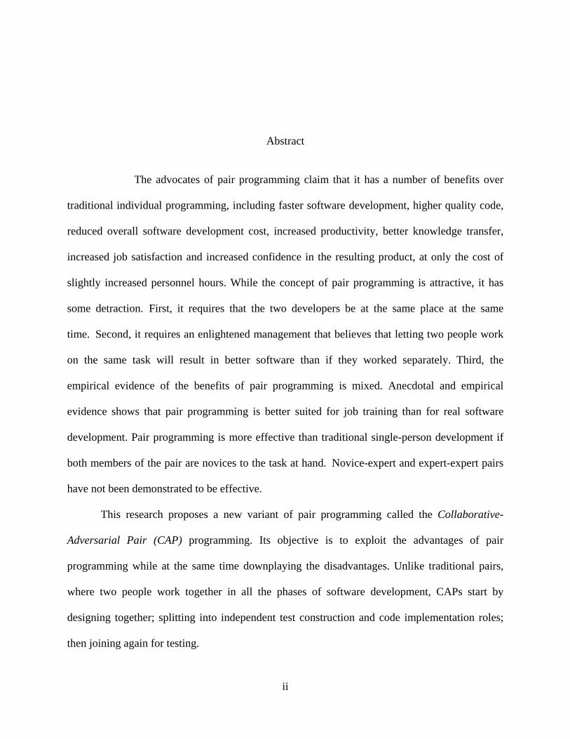
Abstract

The advocates of pair programming claim that it has a number of benefits over

traditional individual programming, including faster software development, higher quality code,

reduced overall software development cost, increased productivity, better knowledge transfer,

increased job satisfaction and increased confidence in the resulting product, at only the cost of

slightly increased personnel hours. While the concept of pair programming is attractive, it has

some detraction. First, it requires that the two developers be at the same place at the same

time. Second, it requires an enlightened management that believes that letting two people work

on the same task will result in better software than if they worked separately. Third, the

empirical evidence of the benefits of pair programming is mixed. Anecdotal and empirical

evidence shows that pair programming is better suited for job training than for real software

development. Pair programming is more effective than traditional single-person development if

both members of the pair are novices to the task at hand. Novice-expert and expert-expert pairs

have not been demonstrated to be effective.

This research proposes a new variant of pair programming called the Collaborative-

Adversarial Pair (CAP) programming. Its objective is to exploit the advantages of pair

programming while at the same time downplaying the disadvantages. Unlike traditional pairs,

where two people work together in all the phases of software development, CAPs start by

designing together; splitting into independent test construction and code implementation roles;

then joining again for testing.

iii

Two empirical experiments were conducted during the Fall 2008 and Spring 2009

semesters to validate CAP against traditional pair programming and individual programming.

Forty two (42) volunteer students, undergraduate seniors and graduate students from Auburn

University’s Software Process class, participated in the studies. The subjects used Eclipse and

JUnit to perform three programming tasks with different degrees of complexity. The subjects

were randomly divided into three experimental groups: individual (Solo) programming group,

pair programming (PP) group and collaborative adversarial pair (CAP) programming group in

the ratio of 1:2:2. The results of this experiment point in favor of CAP development

methodology and do not support the claim that pair programming in general reduces the overall

software development time or increase the program quality or correctness.

iv

To

My wife Uma

and

My guru Dr. David Ashley Umphress

v

Acknowledgments

I consider completing this dissertation to be the greatest accomplishment of my life thus

far. This is a result of sacrifices and encouragement by full many individuals. Although it would

not be possible for me to list them all, I would like to mention a handful without whom this

accomplishment would have remained a dream.

It is with deep sense of gratitude that I acknowledge my indebtedness to my Ph.D.

committee members; in particular, my advisor Dr. David A. Umphress. He has been a wise and

dependable mentor and an exemplary role model in helping me achieve my professional goals.

Dr. Umphress has always given me invaluable guidance, support and enthusiastic

encouragement. Heartfelt thanks are also extended to other committee members, Dr. James Cross

and Dr. Dean Hendrix for their suggestions and guidance which has greatly improved the quality

of my work.

Special thanks goes to all forty two students (fall 2008 and spring 2009 software process

class) who participated in the control experiments. I would also like to thank all the

professors/teachers who have taught me (right from kindergarden to this date) and under whom I

have worked as a Teaching Assistant at Auburn. The inspiration I have drawn from my long list

of friends, right from my childhood to this date, deserves a special acknowledgement. From the

bottom of my heart, I want to thank my parents, my in laws and my extended family for their

love and support. Lastly, I would also like to thank my wife Mrs. Uma Rajendran, my son,

Soorya Gokulan and my daughter Sneha for their love, support and unstinting faith.

vi

Table of Contents

Abstract ......................................................................................................................................... ii

Acknowledgments......................................................................................................................... v

List of Tables ............................................................................................................................. viii

List of Figures .............................................................................................................................. ix

List of Abbreviations ................................................................................................................. xiii

Chapter 1: Introduction ............................................................................................................... 1

Chapter 2: Literature Review ....................................................................................................... 4

2.1. Pair Programming .................................................................................................... 4

2.2. Pair Programming Experiments ............................................................................... 9

2.3. The Pairing Activity ............................................................................................... 23

2.4. The Effect of Pair Programming on Software Development Phases ..................... 35

Chapter 3: Research Description .............................................................................................. 41

3.1. The CAP Process ................................................................................................... 41

Chapter 4: Applied Results and Research Validation ............................................................... 51

4.1. Subjects .................................................................................................................. 51

4.2. Experimental Tasks ................................................................................................ 51

4.3. Hypotheses ............................................................................................................. 52

4.4. Cost ........................................................................................................................ 53

vii

4.5. Program Correctness .............................................................................................. 54

4.6. Experiment Procedure ............................................................................................ 54

4.7. Results .................................................................................................................... 57

4.8. Observations .......................................................................................................... 99

Chapter 5: Applied Results and Research Validation ............................................................. 102

5.1. Conclusions .......................................................................................................... 102

5.2. Future Work ......................................................................................................... 104

References ............................................................................................................................... 105

Appendix A ............................................................................................................................. 111

Appendix B ............................................................................................................................. 113

viii

List of Tables

Table 2.1: Summary of Pair Programming Experiments ........................................................... 19

Table 2.2: Summary of Pair Programming Experiments Results ............................................... 22

Table 2.3: When to Pair Program ............................................................................................... 25

Table 2.4: Effects of Software Processes on PP ......................................................................... 33

Table 2.5: Effects of Programming Languages on PP ............................................................... 34

Table 2.6: Effects of Software Development Methods on PP .................................................... 34

Table 2.7: Summary of Pair Design Experiments ...................................................................... 37

Table 4.1: Total Software Development Time ........................................................................... 62

Table 4.2: Coding Time .............................................................................................................. 64

Table 4.3: The number of test cases passed ................................................................................ 67







Table 4.10: Summary of Control Experiments and their Results ............................................... 98

ix

List of Figures

Figure 2.1: Pair Programming Time Line ..................................................................................... 7

Figure 2.2: The DaimlerChrysler C3 work area ......................................................................... 28

Figure 2.3: Pair Programming Workplace Layout ..................................................................... 29

Figure 2.4: RoleModel Software Workstation Layout .............................................................. 29

Figure 2.5: Conventional Environment....................................................................................... 30

Figure 2.6: Rearranged Environment for Better Role Switching ............................................... 30

Figure 2.7: “Circle table” for pair programming ....................................................................... 31

Figure 3.1: CAP Development Activity ..................................................................................... 42

Figure 3.2: CAP Development Cycle ........................................................................................ 44

Figure 3.3: Collaborative-Adversarial Pairs (CAP) .................................................................... 44

Figure 3.4: Build Code / Unit Implementation in CAP ............................................................. 44

Figure 3.5: A Class-Responsibility-Collaborator (CRC) index card ......................................... 45

Figure 3.6: Unit Test Environment ............................................................................................ 48

Figure 4.1: Experimental Setup .................................................................................................. 56

Figure 4.2: Experimental Procedure .......................................................................................... 56

Figure 4.3: Q-Q Plot of Residuals (Dynamic Pairs Total Software Development Time) ......... 58

Figure 4.4: Q-Q Plot of Residuals (Dynamic Pairs Coding Time) ............................................. 59

Figure 4.5: Test for Normality (Dynamic Pairs Total Software Development Time) ............... 59

Figure 4.6: Test for Normality (Dynamic Pairs Coding Time) ................................................. 59

x

Figure 4.7: Box plot (Dynamic Pairs Total Software Development Time) ............................... 60

Figure 4.8: Box plot (Dynamic Pairs Coding Time) .................................................................. 60

Figure 4.9: Average Total Software Development Time (Dynamic Pairs) ............................... 62

Figure 4.10: Total Software Development Time (Dynamic Pairs) ............................................. 63

Figure 4.11: t-Test Results (Dynamic Pairs Total Software Development Time) ..................... 63

Figure 4.12: Average Coding Time (Dynamic Pairs) ................................................................ 65

Figure 4.13: Box plot (Dynamic Pairs Coding Time) ................................................................ 65

Figure 4.14: t-Test Results (Dynamic Pairs Coding Time) ....................................................... 66

Figure 4.15: The number of test cases passed (Dynamic Pairs) ................................................ 67

Figure 4.16: Q-Q Plot of Residuals (Static Pairs Total Software Development Time) ............. 68

Figure 4.17: Q-Q Plot of Residuals (Static Pairs Coding Time) ................................................ 69

Figure 4.18: Test for Normality (Static Pairs Total Software Development Time) .................. 70

Figure 4.19: Test for Normality (Static Pairs Coding Time) ..................................................... 70

Figure 4.20: Box plot (Static Pairs Total Software Development Time) ................................... 70

Figure 4.21: Box plot (Static Pairs Coding Time) ..................................................................... 71

Figure 4.22: Average Total Software Development Time (Static Pairs) ................................... 73

Figure 4.23: Total Software Development Time (Static Pairs) ................................................. 73

Figure 4.24: t-Test Results (Static Pairs Total Software Development Time) .......................... 74

Figure 4.25: Average Coding Time (Static Pairs) ...................................................................... 75

Figure 4.26: Box plot (Static Pairs Coding Time) ...................................................................... 76

Figure 4.27: Wilcoxon Mann-Whitney U test Results (Static Pairs Coding Time) ................... 76

Figure 4.28: Q-Q Plot of Residuals (Combined CAP Vs PP Total Software Development Time)

..................................................................................................................................................... 77

xi

Figure 4.29: Q-Q Plot of Residuals (Combined CAP Vs PP Coding Time) ............................. 78

Figure 4.30: Test for Normality (Combined CAP Vs PP Total Software Development Time) 78

Figure 4.31: Test for Normality (Combined CAP Vs PP Coding Time) ................................... 79

Figure 4.32: Box plot (Combined CAP Vs PP Total Software Development Time) ................ 79

Figure 4.33: Box plot (Combined CAP Vs PP Coding Time) .................................................... 80

Figure 4.34: Average Total Software Development Time (Combined CAP Vs PP) ................. 81

Figure 4.35: Box Plot (Combined CAP Vs PP Total Software Development Time) ................ 82

Figure 4.36: t-Test Results (Combined CAP Vs PP Total Software Development Time) ........ 83

Figure 4.37: Average Coding Time (Combined CAP Vs PP) ................................................... 84

Figure 4.38: Box plot (Combined CAP Vs PP Coding Time) ................................................... 85

Figure 4.39: Wilcoxon Mann-Whitney U test Result (Combined CAP Vs PP Coding Time) .. 85

Figure 4.40: Q-Q Plot of Residuals (CAP Vs IP Total Software Development Time) ............. 86

Figure 4.41: Q-Q Plot of Residuals (CAP Vs IP Coding Time) ................................................ 87

Figure 4.42: Test for Normality (CAP Vs IP Total Software Development Time) ................... 87

Figure 4.43: Test for Normality (CAP Vs IP Coding Time) ..................................................... 88

Figure 4.44: Box plot (CAP Vs IP Total Software Development Time) ................................... 88

Figure 4.45: Box plot (CAP Vs IP Coding Time) ..................................................................... 89

Figure 4.46: Average Total Software Development Time (CAP Vs IP) .................................... 90

Figure 4.47: Total Software Development Time (CAP Vs IP) .................................................. 91

Figure 4.48: t-Test Results (CAP Vs IP Total Software Development Time) ........................... 92

Figure 4.49: Average Coding Time (CAP Vs IP) ....................................................................... 93

Figure 4.50: Box plot (CAP Vs IP Coding Time) ..................................................................... 94

Figure 4.51: t-Test Results (CAP Vs IP Coding Time) .............................................................. 94

xii

Figure 4.52: Average Software Development Time for Static PP and Dynamic PP .................. 99

Figure 4.53: Average Software Development Time for Static CAP and Dynamic CAP ........ 100

xiii

List of Abbreviations

ANOVA Analysis of variance

BF Brown and Forsythe's variation of Levene's test

C3 Chrysler Comprehensive Compensation

CAP Collaborative-Adversarial Pair Programming

CRC Class Responsibility Collaborator

CSP Collaborative Software Process

GLM General Linear Models

GUI Graphical User Interface

IDE Integrated Development Environment

IP Individual Programming

J2EE Java 2 Platform, Enterprise Edition

JDK Java Development Kit

LOC Lines of Code

OO Object Oriented

PP Pair Programming

PSP Personal Software Process

Q-Q Quintile-Quartile

SAS Statistical Analysis Software

TDD Test Driven Development

xiv

UML Unified Modeling Language

XP Extreme Programming

1

1. INTRODUCTION

One of the popular, emerging, and most controversial topics in the area of Software

Engineering in the recent years is pair programming. Pair programming (PP) is a way of

inspecting code as it is being written. Its premise – that of two people, one computer – is that

two people working together on the same task will likely produce better code than one person

working individually. In pair programming, one person acts as the “driver” and the other person

acts as the “navigator.” The driver is responsible for typing code; the navigator is responsible for

reviewing the code. In a sense, the driver addresses operational issues of implementation and the

observer keeps in mind the strategic direction the code must take.

Though the history of pair programming stretches to punched cards, it gained prominence

in the early 1990’s. It became popular after the publication in 1999 of Extreme Programming

Explained by Kent Beck, where it was noted as one of the 12 key practices promoted by Extreme

Programming (XP) [Beck 2000]. In recent years, industry and academia have turned their

attention and interest toward pair programming [Arisholm et al. 2007, Canfora et al. Dec06] and

it has been widely accepted as an alternative to traditional individual programming [Muller

2005].

The advocates of pair programming claim that it has many benefits over traditional

individual programming, including faster software development, higher quality code, reduced

overall software development cost, increased productivity, better knowledge transfer, increased

2

job satisfaction and increased confidence in their work, only at the cost of slightly increased

personnel hours [Arisholm et al. 2007].

While the concept of pair programming is attractive, it has some detraction. First, it

requires that the two developers be at the same place at the same time. This is frequently not

realistic in busy organizations where developers may be matrixed concurrently to a number of

projects. Second, it requires an enlightened management that believes that letting two people

work on the same task will result in better software than if they worked separately. This is a

significant obstacle since software products are measured more by tangible properties, such as

the number of features implemented, than by intangible properties, such as the quality of the

code. Third, the empirical evidence of the benefits of pair programming is mixed: the works of

Judith Wilson et al. [Wilson et al. 1993], John Nosek [Nosek 1998], Laurie Williams [Williams

et al. 2000], Charlie McDowell et al. [McDowell et al. 2002], and Xu and Rajlich [Xu et al.

2006] support the costs and benefits of pair programming; experiments by Nawrocki and

Wojciechowski [Nawrocki et al. 2001], Jari Vanhanen and Casper Lassenius [Vanhanen et al.

2005], Erik Arisholm et al. [Arisholm et al. 2007], Matevz Rostaher and Marjan Hericko

[Rostaher et al. 2002], and Hanna Hulkko and Pekka Abrahamson [Hulkko et al. 2005] show that

statistically there is no significant difference between the pair programming and solo

programming.

Don Wells and Trish Buckley [Wells et al. 2001], Kim Lui and Keith Chan [Lui et al.

2006] and Erik Arisholm et al. [Arisholm et al. 2007] show that pair programming is more

effective than traditional single-person development if both members of the pair are novices to

the task at hand. Novice-expert and expert-expert pairs have not been demonstrated to be

effective. According to Karl Boutin [Boutin 2000] many developers are forced to abandon pair

3

programming due to lack of resources (e.g. due to small team size). He also observed that

abandoning the pair programming in the middle of the project hindered the integration of new

modules to the existing project.

This research proposes a new variant of pair programming called the Collaborative-

Adversarial Pair (CAP) programming. Its objective is to exploit the advantages of pair

programming while at the same time downplaying the disadvantages. Unlike traditional pairs,

where two people work together in all the phases of software development, CAPs start by

designing together; splitting into independent test construction and code implementation roles;

then joining again for testing.

4

2. LITERATURE REVIEW

2.1. Pair Programming

Pair programming is a programming technique in which two people program all

production code in a single machine using one keyboard and one mouse. The members of each

pair are assigned two different roles. One partner with keyboard and mouse, known as driver1,

types and thinks about the best way to implement the current method in hand and the other

partner, known as navigator or observer, watches or reviews the code being typed, looking for

errors and thinks strategically about the feasibility of the overall approach, additional test cases

to be addressed and the way to simplify the whole system in order to overcome the current

problem [Beck 2000].

The following are some of the key points highlighted in the pair programming literature:

• Paring is dynamic and the people have to pair with different people in the morning and

evening sessions. A programmer can pair with anyone in the development team [Beck

2000].

• Along with writing the code for test cases, the pairs also evolve the system’s design. Pairs

add value to almost all the stages of the system development including analysis,

implementation, and testing [Beck 2000].

1 There were no specific names given for the two partners by Kent Beck in his “Extreme Programming Explained”. The names driver and navigator were originally used by Laurie Williams in her article called “Integrating pair programming into a software development process” [Williams 2001].

5

• The driver and observer are full partners and they exchange their roles quite often [Martin

2003, Wake 2002].

• The pair programming activity provides a means for real-time problem solving and real-

time quality assurance [Pressman 2005].

• Pair programming is a social skill, not a technical skill. It has to be practiced with the

people who already know how to do it [Wells 2001].

• Pair programming is not an activity in which one person programs and other person

simply watches. Moreover, pair programming is not a tutoring activity in which the

experienced partner teaches to the inexperienced ones. It is a conversation between two

people understand together and trying to do simultaneous activity (analysis, design,

implement, or test) [Beck 2000].

Even though the terms collaborative programming (CP) and pair programming (PP) are

interchangeably used in literature, they are not the same. There are two fundamental differences

between them. First there is no working protocol exclusively specified for collaborative

programming; whereas, pair programming has a well defined working protocol which prescribes

to continuously overlapping reviews and the creation of artifacts. Second, pair programming

team is strictly restricted to two people and there is no such restriction for collaborative

programming team; it may contain two or more people [Canfora et al. 2007].

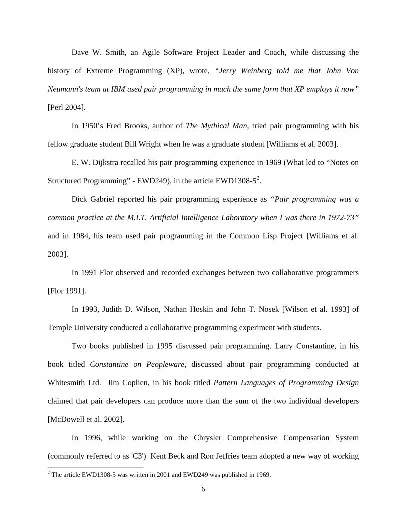
2.1.1. Pair Programming History

The history of pair programming dates back to punched cards in the early 1940s when

Von Neumann worked with IBM. But pair programming became popular only after Kent Beck

published “Extreme Programming Explained” in 1999. The timeline of pair programming is

discussed below:

6

Dave W. Smith, an Agile Software Project Leader and Coach, while discussing the

history of Extreme Programming (XP), wrote, “Jerry Weinberg told me that John Von

Neumann's team at IBM used pair programming in much the same form that XP employs it now”

[Perl 2004].

In 1950’s Fred Brooks, author of The Mythical Man, tried pair programming with his

fellow graduate student Bill Wright when he was a graduate student [Williams et al. 2003].

E. W. Dijkstra recalled his pair programming experience in 1969 (What led to “Notes on

Structured Programming” - EWD249), in the article EWD1308-52.

Dick Gabriel reported his pair programming experience as “Pair programming was a

common practice at the M.I.T. Artificial Intelligence Laboratory when I was there in 1972-73”

and in 1984, his team used pair programming in the Common Lisp Project [Williams et al.

2003].

In 1991 Flor observed and recorded exchanges between two collaborative programmers

[Flor 1991].

In 1993, Judith D. Wilson, Nathan Hoskin and John T. Nosek [Wilson et al. 1993] of

Temple University conducted a collaborative programming experiment with students.

Two books published in 1995 discussed pair programming. Larry Constantine, in his

book titled Constantine on Peopleware, discussed about pair programming conducted at

Whitesmith Ltd. Jim Coplien, in his book titled Pattern Languages of Programming Design

claimed that pair developers can produce more than the sum of the two individual developers

[McDowell et al. 2002].

In 1996, while working on the Chrysler Comprehensive Compensation System

(commonly referred to as 'C3') Kent Beck and Ron Jeffries team adopted a new way of working 2 The article EWD1308-5 was written in 2001 and EWD249 was published in 1969.

7

which is currently known as the Extreme Programming (XP), which employed pair programming

as one of the core principles [Anderson et al. 1998].

Randall W. Jensen, Software Technology Support Center, Hill Air Force Base, reported

his pair programming experience in 1996 as “The undergraduate experience led me to propose

an experiment in the application of what we called two-person programming teams. The term

pair programming had not been coined at that time” [Jensen 2003]3.

In 1998, John T. Nosek, Temple University, Philadelphia, conducted collaborative

programming (similar to pair programming) experiment [Nosek 1998].

In 1999 Kent Beck published Extreme Programming Explained in 1999; pair

programming is the one of the 12 core practices introduced in Extreme Programming [Beck

2000], familiarly known as XP.

Figure 2.1: Pair Programming Time Line

3 The paper was actually published only in 2003.

8

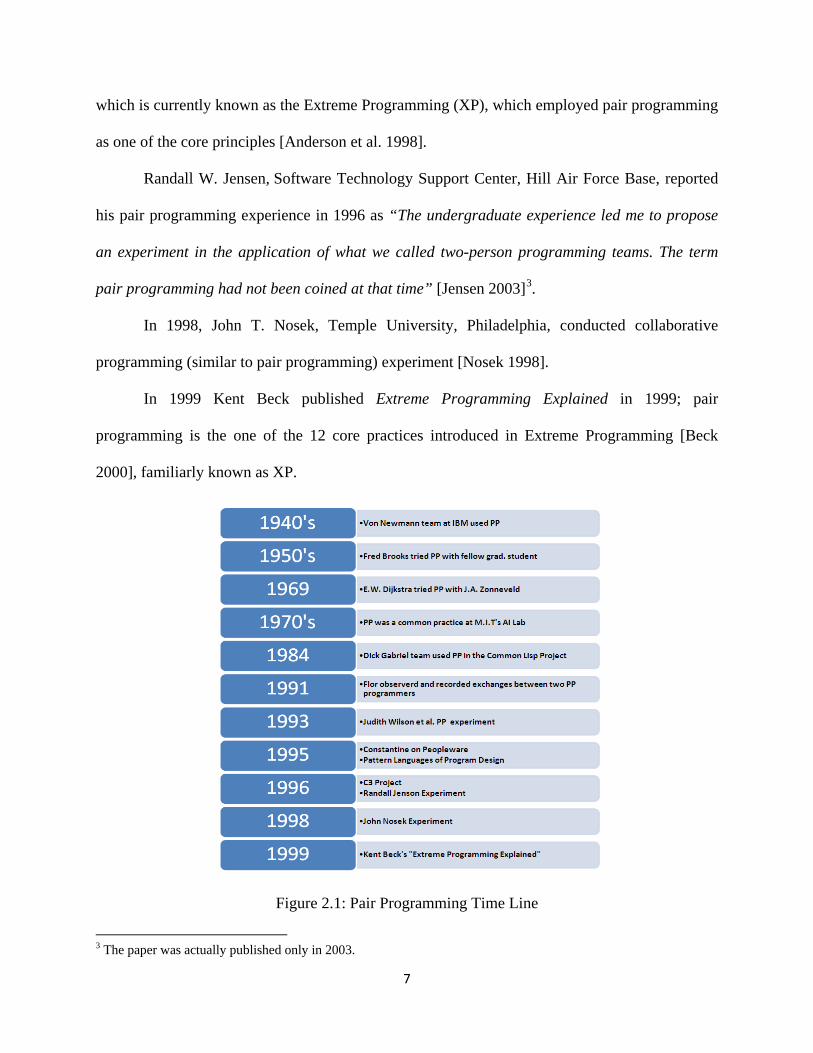
2.1.2. Benefits of Pair Programming

The proponents of pair programming claim that the pair programming software

development provides the following benefits over the traditional individual software

development:

• Increases software quality

• Increases productivity

• Increases design quality

• Increases program correctness

• Provides constant design and code review

• Reduces overall software development time and cost

• Helps in Team building, knowledge transfer and learning

• Enhances job satisfaction and confidence

• Helps in solving complex problems

• Reduces the effort need to develop a piece of code

• Reduces risk of project failures

• Reduces staffing risks

2.1.3. Drawbacks of Pair Programming

While the literature lists several benefits of pair programming, the detractors assert that

pair programming has the following drawbacks:

• Doubles the developers required and development cost

• Increases the software development time

• Quality improvement also in question

• Not suitable for very large projects

9

• Suitable only for novice-novice pairs

• It is very intense

• It is good for job training, not for professional software development

• Bringing out personality conflicts and clashes between developers

• Coding styles, ego, or intimidation would only slow the developers down

• Programming is a solidarity activity

• Experienced programmers may refuse to share

2.2. Pair Programming Experiments

This section includes 12 out of 35 published collaborative and pair programming

experiments and case studies in which (1) a comparison was made between pair programming

and individual programming, and (2) evaluates one or more of the software metrics, namely

program development time/cost, productivity (LOC/hr), program correctness (program

readability and functionality), and job satisfaction. The remaining 23 experiments or case studies

which did not include pairs verses individual comparison, software metrics evaluation and/or

coding phase of the software development process were excluded in this section. For more

information please see Appendix A, which lists all the pair programming experiments and case

studies published so far and the reason why the experiment or case study was excluded from the

analysis.

2.2.1. Judith Wilson et al. Experiment [Wilson et al 1993]

In 1993, Judith D. Wilson, Nathan Hoskin and John T. Nosek of Temple University

conducted a collaborative programming experiment with 34 upper division undergraduate

students of a database course (two sections). 14 students from the first section acted as the

10

control groups (individuals) and 20 students in the second section were randomly grouped into

10 experimental (pairs) groups. The task was solving a “traffic light signal problem” in 60

minutes using Pascal, C, dBase III, or pseudo code.

The purpose of the study was to investigate: (1) readability and functionality of the

solution, (2) confidence and enjoyment of the work, and (3) students in which group earn high

grades. The results of the experiment were: (1) pairs produced slightly better readable and

functional codes, (2) pairs expressed more confidence and enjoyment, and (3) ability had little

effect on pair performance, i.e. high grade is significantly associated with individuals, but not

with pairs.

The experiment indicates that collaboration helps novice programmers, collaboration

helps solve informal problems, and collaboration helps students master analytical skills required

to analyze and model problems.

2.2.2. The Nosek Experiment [Nosek 1998]

John T. Nosek, Temple University, Philadelphia, conducted a collaborative programming

experiment in 1998 using 15 full-time system programmers. The subjects were divided into 5

control groups (individuals) and 5 experimental groups (pairs) on a truly random basis. The task

was to write a database consistency-check script in the C programming language in 45 minutes

on an X-window system.

The aim of the experiment was to find: (1) readability and functionality of the solution,

(2) average problem solving time, (3) confidence and enjoyment of the work, and (4) how

experienced programmers perform as compared to less experienced programmers. The results of

the experiment were: (1) pairs programs were more readable and functional, (2) pairs took more

11

time on average, (3) pairs expressed more confidence and enjoyment of their job, and (4)

experienced programmers performed better than inexperienced ones.

The experiment indicates that collaboration improves problem solving process and

improves programmer’s performance.

2.2.3. Laurie Williams’s Experiment [Williams et al. 2000]

Laurie Williams from University of Utah conducted a Pair Programming experiment in

1999 with 41 advanced undergraduate students in a Software Engineering course. The subjects

were divided into 13 control groups (individuals) and 14 experimental groups (pairs). The

individuals used Humphrey's Personal Software Process (PSP) and the pairs used Williams’

Collaborative Software Process (CSP) to complete their tasks. The subjects were not selected

randomly; instead, they were picked from among the 35 that initially indicated a preference for

working collaboratively. The students were asked to code four class projects4 over 6 weeks time,

which was part of their course curriculum. The first project was used as Pair-Jelling5 (initial

adjustment) experiment.

The aim of the study was to find: (1) number of test cases passed, (2) average problem

solving time, (3) number of defects in the programs, and (4) job satisfaction. The results of the

experiment were: (1) pairs programs passed more test cases than individuals, (2) pairs spent 15%

more time on average to solve a problem, (3) pairs code had 15% fewer defects than individuals,

and (4) pairs expressed more job satisfaction.

4 Programs size and programming language used were not mentioned in the paper. 5 Tuckman’s model (see Appendix B for more detail about Tuckman’s model) is known as Pair Jelling in the pair programming literature [Lui et al. 2006]

12

2.2.4. Nawrocki and Wojciechowski Experiment [Nawrocki et al. 2001]

Jerzy Nawrocki and Adam Wojciechowski from the Poznan University of Technology

conducted a pair programming experiment in the 1999/2000 winter semester using 21 students.

The 21 subjects were randomly divided into three groups of 6, 5 and 5 in such a way that the

average GPA of each group was the same. The first group used Watts Humphrey’s Personal

Software Process (PSP), the second and third groups used Extreme Programming (XP) as their

development process. The individual group which used XP was called XP1 and the pairs group

which used XP was called XP2. The students were asked to solve four C/C++ programs ranges

between 150 and 400 LOC.

The aim of the study was to compare Extreme Programming (XP) with the Watts

Humphrey’s Personal Software Process (PSP). The results of the experiment were: (1) there was

no difference in time between XP1 and XP2 groups, (2) pair programming was more predictable

than other two approaches, (3) XP1 was the most efficient programming technology, and (4)

there was no difference between PSP and XP2.

The experiment indicates that experimentation and test-oriented thinking reduces

development time, pair programming with Extreme Programming (XP) was not efficient, XP1

was more efficient than PSP, pair programming was more predictable than individual

programming, and rework for XP2 was slightly smaller compared with other two approaches.

2.2.5. Charlie McDowell et al. Experiment [McDowell et al. 2002]

In 2000/01, Charlie McDowell, Linda Werner, Heather Bullock and Julian Fernald from

the University of California, Santa Cruz studied the effects of Pair Programming in an

introductory programming course with approximately 600 students. A total of 172 students from

the fall 2000 section were divided into 86 pairs (experimental group) and 141 students from the

13

spring 2001 section were used as control group (individuals). The students were asked to

complete 5 programming assignments6.

The aim of the study was to find the effects of PP on performance in the course. The

results of the experiment were: (1) pair programming improves program quality in terms of

functionality and program readability, and (2) pair programming did not help the students learn

their course material and independently apply their knowledge to new programs.

2.2.6. Rostaher and Hericko Experiment [Rostaher et al. 2002]

In 2002, Matevz Rostaher and Marjan Hericko from Slovenia conducted a pair

programming experiment using 16 professional programmers. The 16 subjects were divided into

4 control groups (individuals) and 6 experimental groups (pairs) based upon their programming

experience. The programmers were asked to develop a simple insurance contract administration

system using six small stories in Smalltalk and its integrated development environment (IDE).

The purpose of the experiment was to get the time spent in percentage on each activity by

the programmers, based on their experience level. The results of the experiment were: (1) there

was no difference in average time spent by individuals and pairs, (2) experiment results did not

favor pair programming.

The experiment indicates that acceptance tests must be written before the development,

and refactoring caused more problems for programmers than did tests.

2.2.7. Muller Experiments [Muller 2005]

Matthias M. Muller, University of Karlsruhe, Germany conducted two experiments to

compare pair programming with peer review. The first experiment was conducted in 2002; in

2003 the same experiment was repeated with 38 computer science students. The 38 subjects were

6 Assignment sizes and programming languages are not mentioned

14

divided into 23 control groups (individuals) called review groups and 19 experimental groups

(pairs). In the review group, an individual programmer developed the program, compiled it, had

it reviewed by an unknown reviewer, and then conducted the testing. In the pair programming

group, all the development activities were carried out by two programmers sitting in front of the

same computer. The students were asked to solve polynomial and shuffle-puzzle problems using

Java on both occasions.

The purpose of the study was to find the cost of pair programming and peer review

methods. The results of the experiment were: (1) there was no difference in program correctness,

and (2) for a similar level of correctness there was no difference in development cost.

The experiment indicates that pair and individual programmers can be interchanged in

terms of cost.

2.2.8. Vanhanen and Lassenius Experiment [Vanhanen et al. 2005]

In 2004, Jari Vanhanen and Casper Lassenius, Helsinki University of Technology,

Finland conducted a pair programming experiment using 10 computer science students. The 10

subjects were randomly divided into 2 control groups (individuals) and 3 experimental groups7

(pairs). For a given requirement specification each team was asked to develop a distributed,

multiplayer casino system within 400 hours using J2EE technologies.

The purpose of the experiment was to investigate pair programming effects, namely

productivity, defects, design quality, knowledge transfer, and enjoyment of work at the

development team level. The results of the experiment were: (1) the productivity of pairs was

29% less than individuals, (2) pairs code contained 8% fewer defects, but after delivery pairs had

more defects, (3) pairs programs were less functional than individual’s programs, (4) pairs

7 In the middle of the project one pair abandoned pair programming without notice because they considered it inefficient.

15

design quality was slightly better than individuals, (5) knowledge transfer among pairs was

better, and (6) pairs expressed less job satisfaction.

The experiment indicates that pair programming did not help in solving complex tasks;

pair programming helped programmers in finding and fixing errors; and fewer defects in

programs and better knowledge transfer among pairs indicates that pair programming may

decrease further development costs of the system.

2.2.9. Hulkko and Abrahamsson Experiments [Hulkko et al. 2005]

Hanna Hulkko and Pekka Abrahamsson from Finland conducted two case studies on pair

programming in 2004. In the first case study, master’s students were the subjects and in the

second case study, master’s students as well as research scientists were the subjects. There were

4 to 6 teams in each control group (individuals) and in each experimental group (pairs), and they

were asked to develop four different projects sizes ranging from 3700 to 7700 LOC using the

Mobile-D8 development process. The first project was developing Internet application using Java

and JSP, and the remaining three were mobile application development using Mobile Java and

Symbian C++.

The purpose of the study was to find the impact of pair programming on product quality.

The results of the experiment were: (1) there was no difference in productivity between pairs and

individuals, (2) pair programming is more suitable for learning and complex tasks, (3) the code

produced by pair programming had lower adherence to coding standard, (4) readability of the

programs were better in pairs code, and (4) there was no difference in program correctness

between pairs and individuals.

8 Mobile-D is an agile development approach developed by Pekka Abrahamsson et al [Abrahamsson et al. 2004]. In this approach development practices are based on Extreme Programming, method scalability is based on Crystal methodologies, and life-cycle coverage is based on Rational Unified Process.

16

The experiment indicates that pair programming did not provide the benefits claimed in

the pair programming literature, and that productivity of pair programming was not consistently

high.

2.2.10. Muller Experiment [Muller 2006]

Matthias M. Muller, University of Karlsruhe, Germany conducted a pair programming

experiment using 18 computer science students. The 18 subjects were randomly divided into 8

control groups (individuals) and 5 experimental groups (pairs). Due the difficult programming

task two individuals did not complete coding, so the modified control group was only 6

individuals. The students were asked to design, code and test an elevator control system using

the Java programming language. Both the control and the experimental groups were initially

paired for the design phase. Once the design was completed with a partner, the control group

students were asked to code and test independently.

The primary purpose of the study was to find the impact of the pair design phase on pair

programming and solo programming. The results of the experiment were: (1) there was no

difference in program correctness, and (2) for a similar level of correctness there was no

difference in development cost.

The experiment indicates: (1) there is no difference in development cost for both pair and

individual programming, if similar level of program correctness is needed and (2) since the

probability of building wrong solution is much lower for pairs, the pair programming process can

be replaced by a pair design phase followed by a solo implementation phase.

2.2.11. Xu and Rajlich Experiment [Xu et al. 2006]

Shaochun Xu from Algoma University College, Laurentine University and Vaclav

Rajlich from Wayne State University conducted a pair programming case study using 12

17

students. The control group was formed using 4 undergraduate computer science students from

Algoma University College and the experimental group was formed using 8 undergraduate

computer science students from Wayne State University. In Feb 2005, two pairs completed their

work and the other two pairs completed their work in Jun 2005. All four individuals completed

their work in Feb 2006.

The participants were asked to develop an application which computes bowling scores.

The pairs were asked to develop the program using the Eclipse Java IDE along with Junit. There

were no such restrictions for the individuals, so two of the four individuals used Eclipse and the

remaining two individuals used Text Pad with the JDK. The pairs were asked to use Extreme

Programming (XP) and Test Driven Development (TDD); whereas the individuals were asked to

use the traditional Waterfall process.

The primary purpose of the study was to investigate the effect of Extreme Programming

and Test Driven Development on game development. The results of the experiment were: (1) the

productivity for pairs was very high compared with individuals, (2) pairs program had better

design than individuals, (3) pairs wrote better quality code than individuals, and (4) pairs

programs passed more test cases than individuals.

The experiment indicates that game developers can benefit from a XP-like approach,

which includes pair programming.

2.2.12. Erick Arisholm et al. Experiment [Arisholm et al. 2007]

Erick Arisholm, Hans Gallis, Tore Dyba, and Dag I.K. Sjoberg conducted a pair

programming experiment using 295 professional programmers from Norway, Sweden, and the

UK. This was a two-phase experiment: the first phase, the individual programming phase, was

conducted in 2001 using 99 programmers and the second phase, the pair programming phase,

18

was conducted in 2004 and 2005 using 196 (98 pairs) programmers. The programmers were

grouped into three categories, namely junior, intermediate, and senior based on an assessment of

their Java programming experience by their project managers. The programmers were asked to

add 4 new features to an existing coffee machine application using professional Java tools.

The primary purpose of the study was to evaluate pair programming with respect to

system complexity and programmer expertise. The results of the experiment were: (1) there was

no difference in development time between pairs and individuals, (2) there was no difference in

program correctness between pair and individual programs, and (3) pairs required more effort

than individuals to add new features.

The experiment indicates that the effect of pair programming on duration, effort and

correctness depends on system complexity and not on programmer’s expertise. The juniors were

the beneficiaries from the pair programming and there was no benefit for intermediates and

seniors from pair programming.

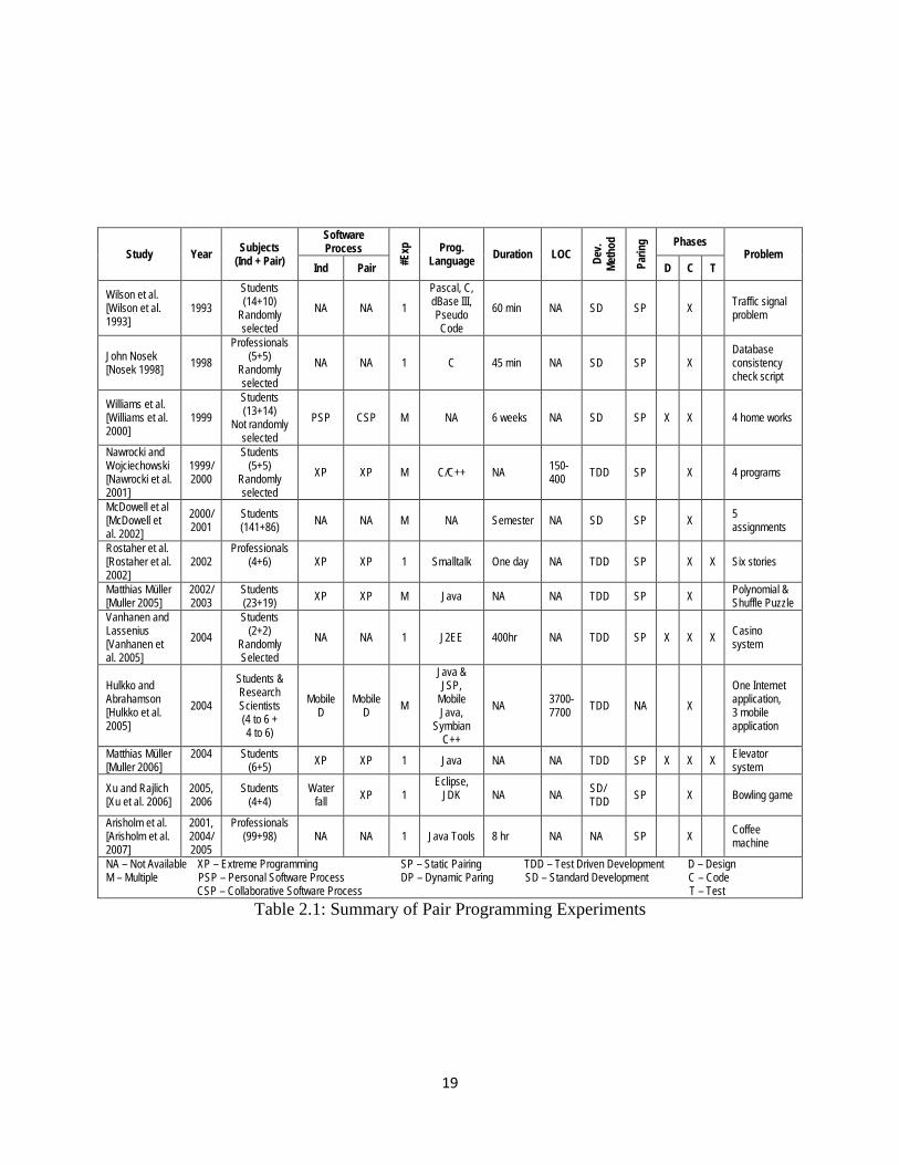
2.2.13. Summary of PP Experiments

Twelve pair programming experiments have been discussed in section 2.2.1 through

2.2.12. A synopsis of these experiments highlighting the name and year of the experiment,

number of participants in the experiment, software process used, number of problems solved,

programming language used, duration of experiment, lines of code, development methodology

used, phases paired, and the experimental problem solved is shown in table 2.1.

19

Study Year Subjects (Ind + Pair)

Software Process

#Exp

Prog. Language Duration LOC De

v.

Meth

od

Parin

g Phases Problem

Ind Pair D C T

Wilson et al. [Wilson et al. 1993]

1993 Students (14+10)

Randomly selected

NA NA 1 Pascal, C, dBase III, Pseudo Code

60 min NA SD SP X Traffic signal problem

John Nosek [Nosek 1998] 1998

Professionals (5+5)

Randomly selected

NA NA 1 C 45 min NA SD SP X Database consistency check script

Williams et al. [Williams et al. 2000]

1999 Students (13+14)

Not randomly selected

PSP CSP M NA 6 weeks NA SD SP X X 4 home works

Nawrocki and Wojciechowski [Nawrocki et al. 2001]

1999/ 2000

Students (5+5)

Randomly selected

XP XP M C/C++ NA 150- 400 TDD SP X 4 programs

McDowell et al [McDowell et al. 2002]

2000/ 2001

Students (141+86) NA NA M NA Semester NA SD SP X 5

assignments

Rostaher et al. [Rostaher et al. 2002]

2002 Professionals

(4+6)

XP XP 1 Smalltalk One day NA TDD SP X X Six stories

Matthias Müller [Muller 2005]

2002/ 2003

Students (23+19) XP XP M Java NA NA TDD SP X Polynomial &

Shuffle Puzzle Vanhanen and Lassenius [Vanhanen et al. 2005]

2004 Students

(2+2) Randomly Selected

NA NA 1 J2EE 400hr NA TDD SP X X X Casino system

Hulkko and Abrahamson [Hulkko et al. 2005]

2004

Students & Research Scientists (4 to 6 + 4 to 6)

Mobile D

Mobile D M

Java & JSP,

Mobile Java,

Symbian C++

NA 3700- 7700 TDD NA X

One Internet application, 3 mobile application


2004

Students (6+5) XP XP 1 Java NA NA TDD SP X X X Elevator

system

Xu and Rajlich [Xu et al. 2006]

2005, 2006

Students (4+4)

Water fall XP 1

Eclipse, JDK

NA NA SD/

TDD SP X Bowling game

Arisholm et al. [Arisholm et al. 2007]

2001, 2004/ 2005

Professionals (99+98)

NA NA 1 Java Tools 8 hr NA NA SP X Coffee

machine

NA – Not Available XP – Extreme Programming SP – Static Pairing TDD – Test Driven Development D – Design M – Multiple PSP – Personal Software Process DP – Dynamic Paring SD – Standard Development C – Code CSP – Collaborative Software Process T – Test

Table 2.1: Summary of Pair Programming Experiments

20

Programming efficiency or productivity is the measure of Line of Code (LOC) produced

per hour per programmer. Nawrocki and Wojciechowski [Nawrocki et al. 2001], Vanhanen and

Lassenius [Vanhanen et al. 2005] and Hulkko and Abrahamson [Hulkko et al. 2005] show that

the productivity of the pair programmers was not more than the individual programmers

productivity; the only exception to this is the Xu and Rajlich [Xu et al. 2006] experiment.

John Nosek [Nosek 1998], Williams et al. [Williams et al. 2000], Nawrocki and

Wojciechowski [Nawrocki et al. 2001], Rostaher et al. [Rostaher et al. 2002], Matthias Müller

[Muller 2005], Xu and Rajlich [Xu et al. 2006], and Arisholm et al. [Arisholm et al. 2007] show

that the time taken by the pair programmers to complete a task was more than the time taken by

the individual programmers. Moreover, Nawrocki and Wojciechowski [Nawrocki et al. 2001]

and Rostaher et al. [Rostaher et al. 2002] show that pairs took almost double the time than

individual programmers.

The defect density is measured in terms of number of test cases passed [Williams et al.

2000, Xu et al. 2006] and/or relative defect density (defects/KLOC) [Williams et al. 2000,

Hulkko et al. 2005]. Williams et al. [Williams et al. 2000] and Xu and Rajlich [Xu et al. 2006]

show that the number of test cases passed by pairs programs were higher than individual

programmers. Matthias Müller [Muller 2005] shows that programs written by pair groups and

review groups have similar level of correctness. Arisholm et al. [Arisholm et al. 2007] report that

the pairs did not produce more correct programs than individuals. Vanhanen and Lassenius

[Vanhanen et al. 2005] report that after coding and unit testing the programs written by pairs had

less defects; whereas, after the system testing and bug fixing the programs written by pairs had

more defects than individuals.

21

Williams et al. [Williams et al. 2000] report that pairs programs had less defect density,

but Hulkko and Abrahamson [Hulkko et al. 2005] show that pairs produced code with more

defect density.

Wilson et al. [Wilson et al. 1993] and John Nosek [Nosek 1998] measure the code quality

in terms of its functionality, the number of software components contained in the program, and

readability, the number of comments the program contains; whereas, Xu and Rajlich [Xu et al.

2006] measured the code quality in terms of its elegances and readability.

Xu and Rajlich [Xu et al. 2006] show that the programs written by pairs were more

readable and elegance, but Wilson et al. [Wilson et al. 1993] and John Nosek [Nosek 1998] show

that statistically there was no significant difference in readability between the individual and pair

programmers codes.

With respect to functionality the John Nosek [Nosek 1998] experiment shows that pair

programs were more functional, whereas, in the Wilson et al. [Wilson et al. 1993] experiment,

the individual programmers programs were more functional than pairs.

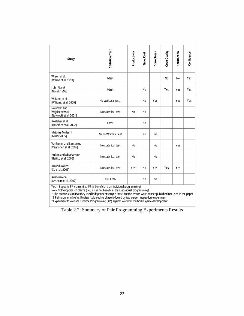
Based on the post experiment survey the experimenters calculate the programmer’s job

satisfaction and confidence on their work. John Nosek [Nosek 1998], Williams et al. [Williams

et al. 2000], Vanhanen and Lassenius [Vanhanen et al. 2005], Xu and Rajlich [Xu et al. 2006]

and Wilson et al. [Wilson et al. 1993] show that pairs expressed their satisfaction over pair

programming. Wilson et al. [Wilson et al. 1993], John Nosek [Nosek 1998], and Williams et al.

[Williams et al. 2000] show that pairs expressed their confidence on their work when using pair

programming. The results of the above mentioned experiments with respect to the efficacy of

pair programming are shown in table 2.2.

22

Study

Stat

istica

l Tes

t

Prod

uctiv

ity

Tim

e /Co

st

Corre

ctne

ss

Code

Qua

lity

Satis

fact

ion

Conf

iden

ce

Wilson et al. [Wilson et al. 1993] t-test No No Yes

John Nosek [Nosek 1998] t-test No Yes Yes Yes

Williams et al. [Williams et al. 2000] No statistical test† No Yes Yes Yes


No statistical test No No

Rostaher et al. [Rostaher et al. 2002] t-test No

Matthias Müller†† [Muller 2005] Mann-Whitney Test No No

Vanhanen and Lassenius [Vanhanen et al. 2005] No statistical test No No Yes

Hulkko and Abrahamson [Hulkko et al. 2005] No statistical test No No

Xu and Rajlich* [Xu et al. 2006] No statistical test Yes No Yes Yes Yes

Arisholm et al. [Arisholm et al. 2007] ANCOVA No No

Yes – Supports PP claims (i.e., PP is beneficial than Individual programming) No – Not Supports PP claims (i.e., PP is not beneficial than Individual programming) † The authors claim that they used independent sample t-test, but the results were neither published nor used in the paper †† Pair programming Vs Review (solo coding phase followed by two person inspection) experiment * Experiment to validate Extreme Programming (XP) against Waterfall method in game development

Table 2.2: Summary of Pair Programming Experiments Results

23

2.3. The Pairing Activity

While much of the literature explains what pair programming is, it fails to answer some

key questions:

• When to pair program?

• How to form pairs?

• How frequently partners have to switch their roles?

• When to exchange the partners?

• What the working environment should look like?

• Who owns the task at hand – the pair or a person?

• Who owns the code?

• Whether Extreme Programming or pair programming denies specialists?

• What is the role of programming languages and tools in pair programming?

2.3.1. When to Pair Program?

John Nosek [Nosek 1998] suggests that pair programming might be preferred over

individual programming in situations like (1) speeding up development – if the organization

wants to bring its product earlier to market for it to gain an edge over its competitors and (2)

improving software quality – to produce a high quality product, which has very high profit

margin. Thus pair programming is preferred when the organization need to develop high quality

products in short time. Matthias Muller [Muller 2005] suggests that pair programming is a viable

option for developing software with fewer failures.

Judith Wilson et al. [Wilson et al. 1993], Don Wells and Trish Buckley [Wells et al.

2001], Kim Lui and Keith Chan [Lui et al. 2006], and Erik Arisholm et al. [Arisholm et al. 2007]

observe that novice programmers benefit from pair programming. Don Wells and Trish Buckley

24

[Wells et al. 2001] observe that novice-novice pairs work better than expert-novice pairs,

because the novices feel that they are not intimidated and demoralized. Moreover the novices

learned from each other while solving the problem. Don Wells and Trish Buckley [Wells et al.

2001] also suggest that people with equal experience should pair in order to achieve significant

productivity and morale.

Studies by Jari Vanhanen and Casper Lassenius [Vanhanen et al. 2005] and Hanna

Hulkko and Pekka Abrahamsson [Hulkko et al. 2005] show that pair programming helps in

transferring the knowledge about the system among the team members; meaning, it enhances

training.

Studies by Hanna Hulkko and Pekka Abrahamsson [Hulkko et al. 2005], Erik Arisholm

et al. [Arisholm et al. 2007], Benedicenti and Paranjape [Benedicenti et al. 2001], Becker-Pechau

et al. [Pechau et al.2003] and Gittins et al. [Gittins et al. 2001] show that pair programming is

useful with complex tasks. Moreover, Erik Arisholm et al. [Arisholm et al. 2007] suggest that

pair programming is effective when assigning complex maintenance tasks to junior

programmers. Jari Vanhanen and Casper Lassenius [Vanhanen et al. 2005], on the other hand,

show that pair programming does not help in solving complex tasks.

Xu and Rajlich quote Kent Beck [Beck 2000] as stating “that pair programming (or XP)

is not suitable for very large projects” [Xu et al. 2006].

Ambu and Gianneschi [Ambu et al. 2003] suggest that pair programming is not suitable

with tight deadlines.

Pair programming is not possible if the development team size is small [Boutin 2000].

Karl Boutin [Boutin 2000] reported that in his research and development lab the developers were

forced to abandon pair programming due to lack of resources (i.e. due to small team size). At the

25

same time Kent Beck [Beck 2000] suggests that XP is not possible when the development team

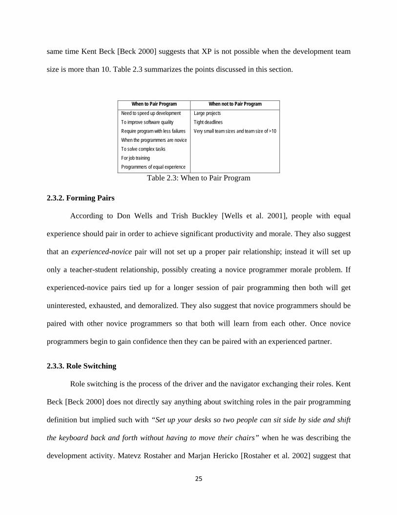
size is more than 10. Table 2.3 summarizes the points discussed in this section.

When to Pair Program When not to Pair Program

Need to speed up development To improve software quality Require program with less failures When the programmers are novice To solve complex tasks For job training Programmers of equal experience

Large projects Tight deadlines Very small team sizes and team size of >10

Table 2.3: When to Pair Program

2.3.2. Forming Pairs

According to Don Wells and Trish Buckley [Wells et al. 2001], people with equal

experience should pair in order to achieve significant productivity and morale. They also suggest

that an experienced-novice pair will not set up a proper pair relationship; instead it will set up

only a teacher-student relationship, possibly creating a novice programmer morale problem. If

experienced-novice pairs tied up for a longer session of pair programming then both will get

uninterested, exhausted, and demoralized. They also suggest that novice programmers should be

paired with other novice programmers so that both will learn from each other. Once novice

programmers begin to gain confidence then they can be paired with an experienced partner.

2.3.3. Role Switching

Role switching is the process of the driver and the navigator exchanging their roles. Kent

Beck [Beck 2000] does not directly say anything about switching roles in the pair programming

definition but implied such with “Set up your desks so two people can sit side by side and shift

the keyboard back and forth without having to move their chairs” when he was describing the

development activity. Matevz Rostaher and Marjan Hericko [Rostaher et al. 2002] suggest that

26

role switching rhythm (the high frequency of role switching, more than 20 times per day, and

short phases of uninterrupted activity, 5 minutes in average) is essential for test-first pair

programming.

According to William Wake [Wake 2002], role switching can be done every couple of

minutes or a few times an hour. Robert Martin suggests that whenever the driver gets tired or

stuck, the navigator should take over the driver’s job. This is normally happens several times an

hour.

Matevz Rostaher and Marjan Hericko [Rostaher et al. 2002] observed that role switching

occurred 21 times per day on average for all programmers and 42 times per day on average for

experienced programmers. They also observed that uninterrupted activity lasted 5 minutes in

average for all programmers and 3 minutes for experienced programmers. Lippert et al. [Lippert

et al. 2001] observed that the physical working environment (seating arrangement) plays a

crucial part in role switching. Conventional seating arrangement hinders the frequent role

switching. Once the seating is rearranged, pairs switch their roles more frequently (the seating

arrangement is discussed more detail in section 2.3.5).

2.3.4. Partner Exchange

The main idea behind rotating developers among different pairs is to spread the system

knowledge to every member of the development team.

Kent Beck [Beck 2000] says “Paring is dynamic”, meaning, people have to pair with

different people in the morning and evening sessions, and a programmer can pair with anyone in

the development team. William Wake [Wake 2002] suggests that the developers have to

exchange their partners every day and some developers will exchange their partners more often

depending upon the situation. Robert Martin [Martin 2003] suggests that every member of the

27

development team should try all the activities of the current iteration and that he/she has to

partner with every member in the team. He also suggests that every programmer has to work in

at least in two different pairs.

2.3.5. Workplace Layout

To emphasize the importance of the workplace layout for pair programming’s success in

DaimlerChrysler C3 project, Kent Beck [Beck 2000] writes “I was brought in because of my

knowledge of Smalltalk and objects, and the most valuable suggestion I had was that they should

rearrange the furniture”.

According to Kent Beck [Beck 2000], a reasonable work place is important for any

project’s success. Kent Beck [Beck 2000] and Lippert et al. [Lippert et al. 2001] suggest that the

physical environment (i.e., the desk and seating arrangement) plays a critical role in pair

programming. This was confirmed by the result of the survey conducted by Laurie Williams and

Robert Kessler [Williams et al. 2000b] in which 96% of the programmers agreed that proper

workplace layout was critical to their pair programming success. Lippert et al. [Lippert et al.

2001] also observed that the conventional seating arrangement hindered the frequent role

switching, and once the seating was rearranged, the pairs switched their roles more frequently.

For the success of pair programming, developers need to communicate with their partners

and with other members of the team as well [Beck 2000, Williams et al. 2003]. The pair

programming layout must be arranged in such a way that it allows inter-pair and intra-pair

communications.

28

Kent Beck [Beck 2000] defines the working environment for pair programming as

follows:

“Common office layouts don't work well for XP. Putting your computer in a corner, for example, doesn't work, because it is impossible for two people to sit side-by-side and program. Ordinary cubicle wall heights don't work well—walls between cubicles should be half-height or eliminated entirely. At the same time, the team should be separated from other teams”. “One big room with little cubbies around the outside and powerful machines on tables in the middle is about the best environment I know”.

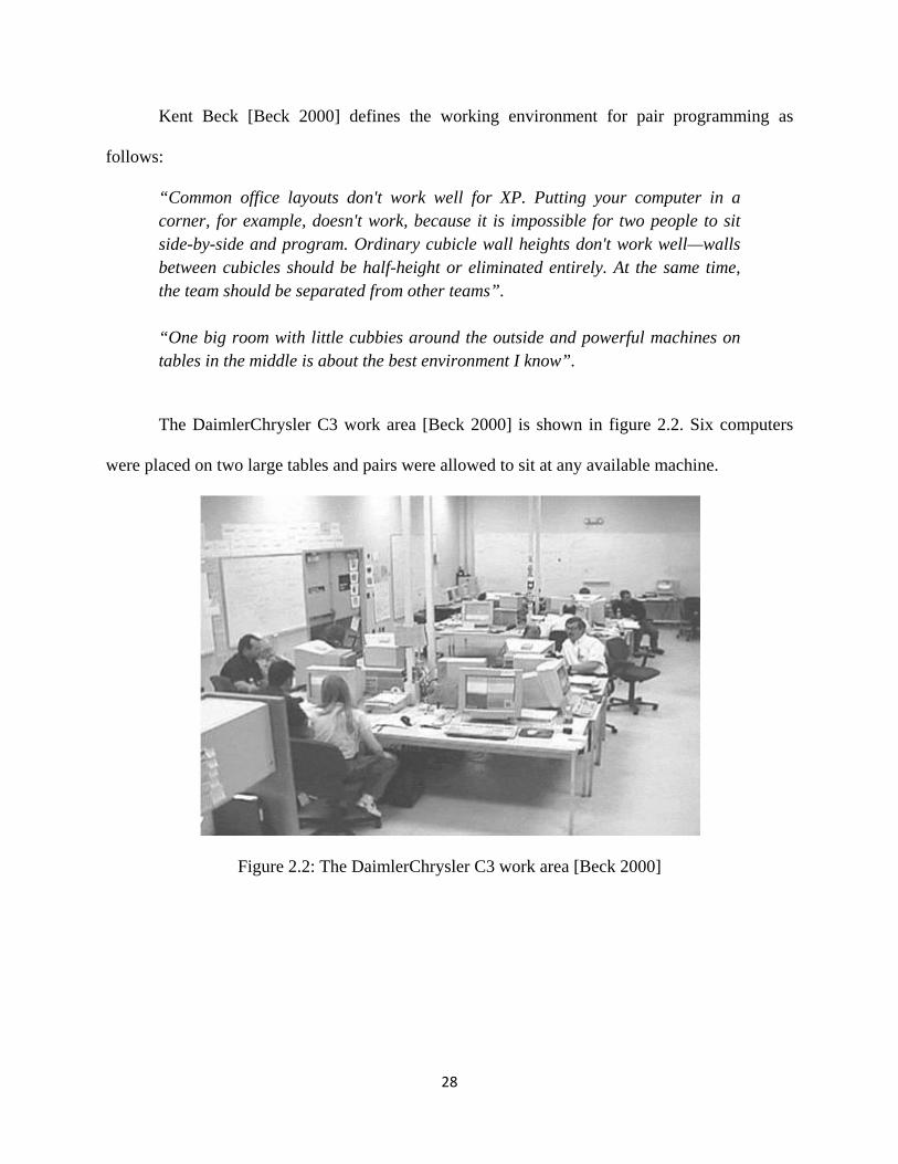
The DaimlerChrysler C3 work area [Beck 2000] is shown in figure 2.2. Six computers

were placed on two large tables and pairs were allowed to sit at any available machine.

Figure 2.2: The DaimlerChrysler C3 work area [Beck 2000]

29

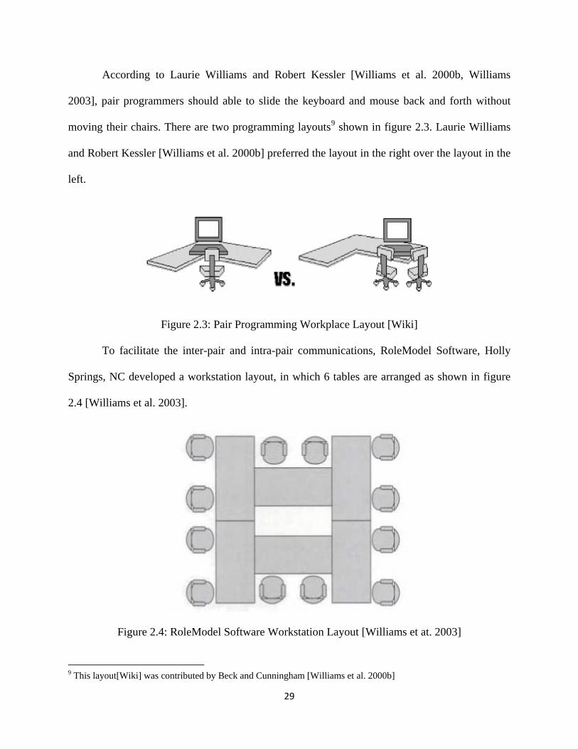
According to Laurie Williams and Robert Kessler [Williams et al. 2000b, Williams

2003], pair programmers should able to slide the keyboard and mouse back and forth without

moving their chairs. There are two programming layouts9 shown in figure 2.3. Laurie Williams

and Robert Kessler [Williams et al. 2000b] preferred the layout in the right over the layout in the

left.

Figure 2.3: Pair Programming Workplace Layout [Wiki]

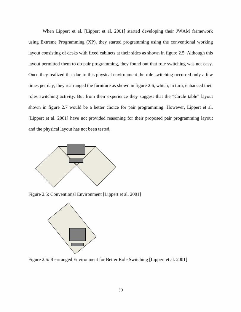
To facilitate the inter-pair and intra-pair communications, RoleModel Software, Holly

Springs, NC developed a workstation layout, in which 6 tables are arranged as shown in figure

2.4 [Williams et al. 2003].

Figure 2.4: RoleModel Software Workstation Layout [Williams et at. 2003]

9 This layout[Wiki] was contributed by Beck and Cunningham [Williams et al. 2000b]

30

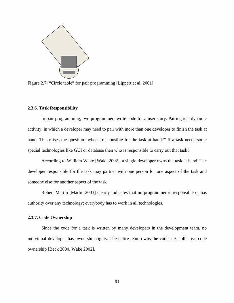
When Lippert et al. [Lippert et al. 2001] started developing their JWAM framework

using Extreme Programming (XP), they started programming using the conventional working

layout consisting of desks with fixed cabinets at their sides as shown in figure 2.5. Although this

layout permitted them to do pair programming, they found out that role switching was not easy.

Once they realized that due to this physical environment the role switching occurred only a few

times per day, they rearranged the furniture as shown in figure 2.6, which, in turn, enhanced their

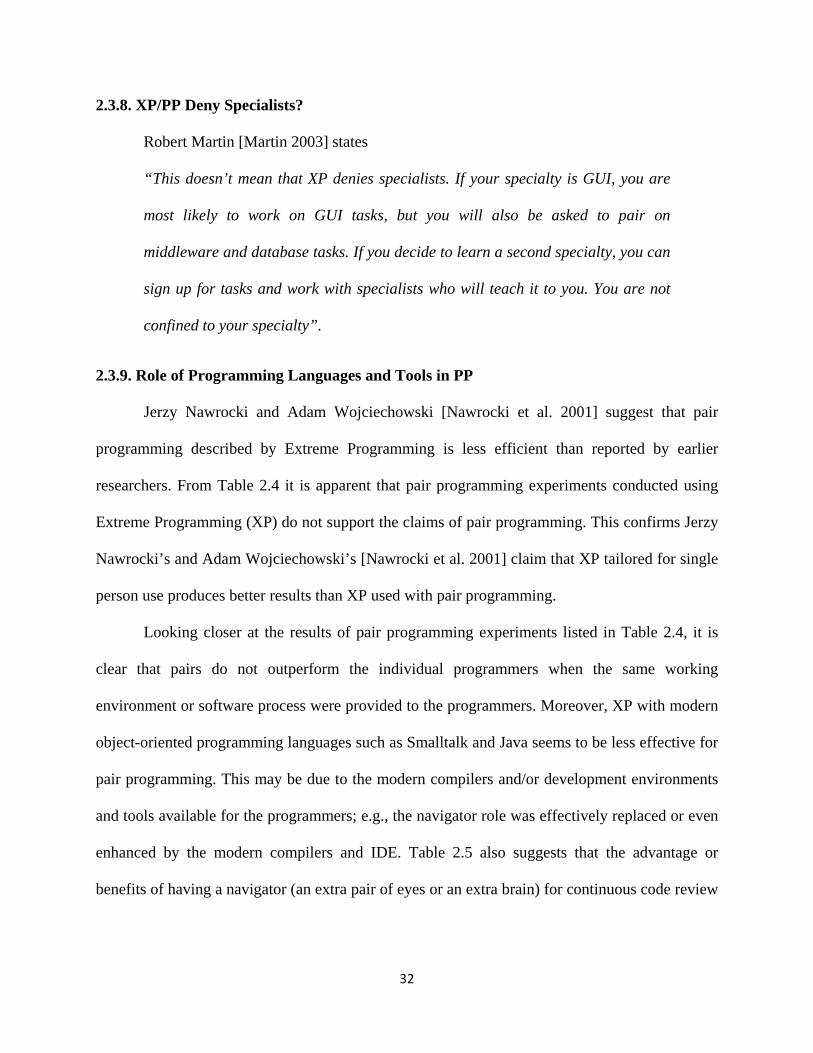
roles switching activity. But from their experience they suggest that the “Circle table” layout

shown in figure 2.7 would be a better choice for pair programming. However, Lippert et al.

[Lippert et al. 2001] have not provided reasoning for their proposed pair programming layout

and the physical layout has not been tested.

Figure 2.5: Conventional Environment [Lippert et al. 2001]

Figure 2.6: Rearranged Environment for Better Role Switching [Lippert et al. 2001]

31

Figure 2.7: “Circle table” for pair programming [Lippert et al. 2001]

2.3.6. Task Responsibility

In pair programming, two programmers write code for a user story. Pairing is a dynamic

activity, in which a developer may need to pair with more than one developer to finish the task at

hand. This raises the question “who is responsible for the task at hand?” If a task needs some

special technologies like GUI or database then who is responsible to carry out that task?

According to William Wake [Wake 2002], a single developer owns the task at hand. The

developer responsible for the task may partner with one person for one aspect of the task and

someone else for another aspect of the task.

Robert Martin [Martin 2003] clearly indicates that no programmer is responsible or has

authority over any technology; everybody has to work in all technologies.

2.3.7. Code Ownership

Since the code for a task is written by many developers in the development team, no

individual developer has ownership rights. The entire team owns the code, i.e. collective code

ownership [Beck 2000, Wake 2002].

32

2.3.8. XP/PP Deny Specialists?

Robert Martin [Martin 2003] states

“This doesn’t mean that XP denies specialists. If your specialty is GUI, you are

most likely to work on GUI tasks, but you will also be asked to pair on

middleware and database tasks. If you decide to learn a second specialty, you can

sign up for tasks and work with specialists who will teach it to you. You are not

confined to your specialty”.

2.3.9. Role of Programming Languages and Tools in PP

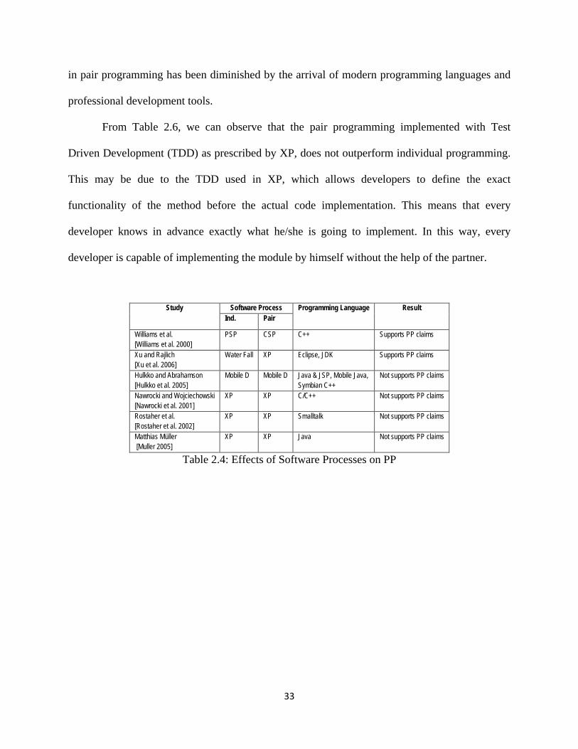
Jerzy Nawrocki and Adam Wojciechowski [Nawrocki et al. 2001] suggest that pair

programming described by Extreme Programming is less efficient than reported by earlier

researchers. From Table 2.4 it is apparent that pair programming experiments conducted using

Extreme Programming (XP) do not support the claims of pair programming. This confirms Jerzy

Nawrocki’s and Adam Wojciechowski’s [Nawrocki et al. 2001] claim that XP tailored for single

person use produces better results than XP used with pair programming.

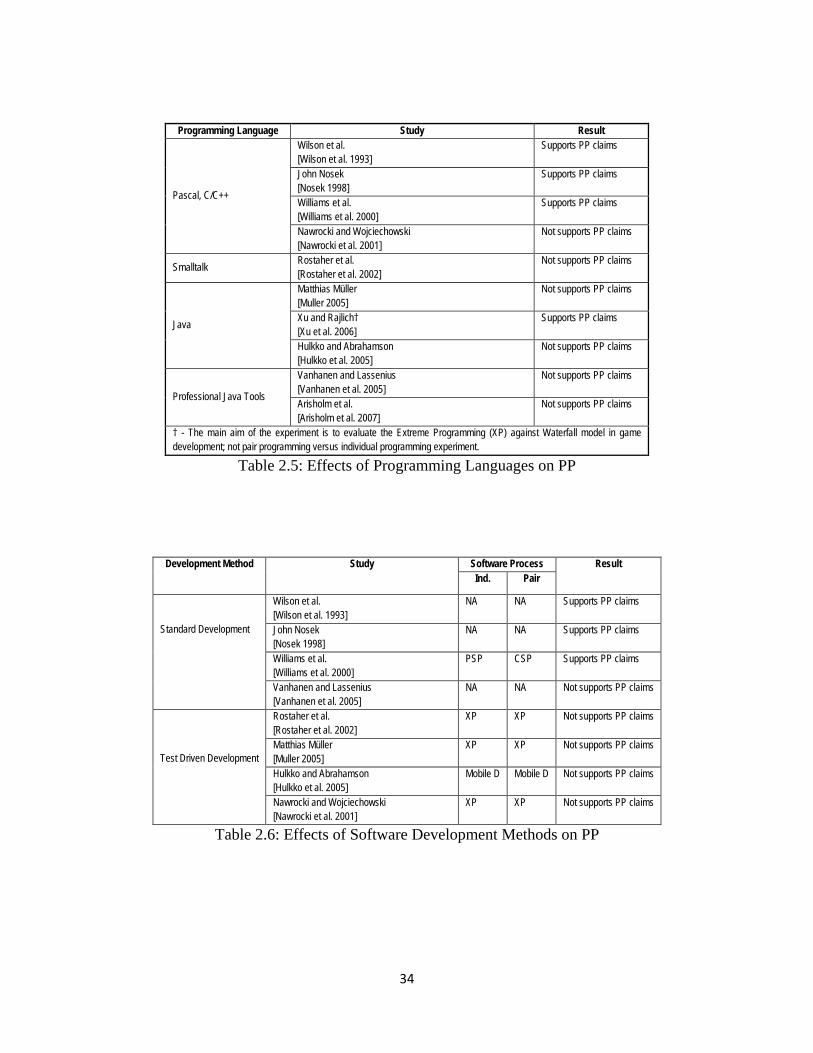
Looking closer at the results of pair programming experiments listed in Table 2.4, it is

clear that pairs do not outperform the individual programmers when the same working

environment or software process were provided to the programmers. Moreover, XP with modern

object-oriented programming languages such as Smalltalk and Java seems to be less effective for

pair programming. This may be due to the modern compilers and/or development environments

and tools available for the programmers; e.g., the navigator role was effectively replaced or even

enhanced by the modern compilers and IDE. Table 2.5 also suggests that the advantage or

benefits of having a navigator (an extra pair of eyes or an extra brain) for continuous code review

33

in pair programming has been diminished by the arrival of modern programming languages and

professional development tools.

From Table 2.6, we can observe that the pair programming implemented with Test

Driven Development (TDD) as prescribed by XP, does not outperform individual programming.

This may be due to the TDD used in XP, which allows developers to define the exact

functionality of the method before the actual code implementation. This means that every

developer knows in advance exactly what he/she is going to implement. In this way, every

developer is capable of implementing the module by himself without the help of the partner.

Study Software Process Programming Language Result Ind. Pair


PSP CSP C++ Supports PP claims

Xu and Rajlich [Xu et al. 2006]

Water Fall XP Eclipse, JDK Supports PP claims


Mobile D Mobile D Java & JSP, Mobile Java, Symbian C++

Not supports PP claims


XP XP C/C++ Not supports PP claims


XP XP Smalltalk Not supports PP claims


XP XP Java Not supports PP claims

Table 2.4: Effects of Software Processes on PP

34

Programming Language Study Result

Pascal, C/C++


Supports PP claims

John Nosek [Nosek 1998]

Supports PP claims


Supports PP claims



Smalltalk Rostaher et al. [Rostaher et al. 2002]


Java



Xu and Rajlich† [Xu et al. 2006]

Supports PP claims



Professional Java Tools

Vanhanen and Lassenius [Vanhanen et al. 2005]


Arisholm et al. [Arisholm et al. 2007]


† - The main aim of the experiment is to evaluate the Extreme Programming (XP) against Waterfall model in game development; not pair programming versus individual programming experiment.

Table 2.5: Effects of Programming Languages on PP

Development Method Study Software Process Result Ind. Pair

Standard Development


NA NA Supports PP claims

John Nosek [Nosek 1998]

NA NA Supports PP claims


PSP CSP Supports PP claims

Vanhanen and Lassenius [Vanhanen et al. 2005]

NA NA Not supports PP claims

Test Driven Development


XP XP Not supports PP claims




Mobile D Mobile D Not supports PP claims



Table 2.6: Effects of Software Development Methods on PP

35

2.4. The Effect of Pair Programming on Software Development Phases

One of the basic requirements of pair programming is that all production code must be

programmed by pairs, which, in turn, doubles the developers required to complete a project and

also almost doubles the development cost. Unquestionably this is a waste of resource; though the

proponents of pair programming claim that “pair programming increases initial development

time but saves time in the long run because there are fewer defects” [Cockburn et al. 2000]. Up

to now there is no empirical evidence for their claim. Because the amount of skill required to

carry out the various phases of software process are different, there is no guarantee that pair

programming will produce the same results in all the phases. The results of the Hanna Hulkko

and Pekka Abrahamson [Hulkko et al. 2005] case studies suggest that pair programming was

more useful in the beginning of the project and that the pair programming effort steadily

decreased in the subsequent iterations and again increased in the final iteration (defect correction

after system test).

The main aim of this section is to explore whether pairing up of developers is required in

all the phases of software development, or if there an alternate way to minimize the pair-up times

between these developers, in order to maximize the resource utilization and reduce the

development cost.

2.4.1. Pair Design

Due to the asymmetrical nature of the design and code phases, we cannot expect all the

benefits of pair-coding to apply to pair-design as well [Canfora et al. Sep 06]. Various studies

highlight the benefits of pair-design. According to Laurie Williams et al. [Williams et al. 2000],

pair-analysis and pair-design are more critical than pair-implementation, and pair-analysis and

36

pair-design are critical for pair success. They also state that “It is doubtless true that two brains

are better than one when performing analysis and design”.

Emilio Bellini et al. [Bellini et al. 2005] reveal that pair-design was more predictable than

individual design and helped the developers to understand the system while developing it. This

learned knowledge about the system can help developers in developing the project with less

rework.

The pair-design experiment conducted by Gerardo Canfora et al. [Canfora et al. Sep 06]

in September 2006, suggests that pair-design will also produce all anticipated benefits of pair-

coding. Their experimental results show that pairs produced better design in less time than

individuals. Moreover, with respect to effort and quality, the pair design was more predictable

than individual design (i.e. the standard deviation of pair metrics was smaller than the one of

solos). They also suggest that the industry can use pair design in critical situations and also in

situations with short deadlines, lack of resources, and lack of skilled personnel. The pair design

experiment conducted by Gerardo Canfora et al. [Canfora et al. Dec 06] in December 2006,

suggests that pair design slows down the task but improves quality. They also found that the

quality of pair design was more predictable (i.e. the standard deviation obtained by pairs was

smaller than the one of solos) than individual design quality.

Matthias M. Muller [Muller 2006] conducted a pair programming experiment using 18

computer science students. The 18 subjects were randomly divided into 8 control groups

(individuals) and 5 experimental groups (pairs). The students were asked to design, code and test

an elevator control system using Java. Both control and experimental groups were initially paired

for the design phase. Once the design was completed with the partner, the control group students

were asked to code and test independently. The results show that the costly pair programming

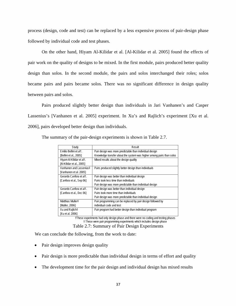
37

process (design, code and test) can be replaced by a less expensive process of pair-design phase

followed by individual code and test phases.

On the other hand, Hiyam Al-Kilidar et al. [Al-Kilidar et al. 2005] found the effects of

pair work on the quality of designs to be mixed. In the first module, pairs produced better quality

design than solos. In the second module, the pairs and solos interchanged their roles; solos

became pairs and pairs became solos. There was no significant difference in design quality

between pairs and solos.

Pairs produced slightly better design than individuals in Jari Vanhanen’s and Casper

Lassenius’s [Vanhanen et al. 2005] experiment. In Xu’s and Rajlich’s experiment [Xu et al.

2006], pairs developed better design than individuals.

The summary of the pair-design experiments is shown in Table 2.7.

Study Result Emilio Bellini et al†. [Bellini et al., 2005]

Pair design was more predictable than individual design Knowledge transfer about the system was higher among pairs than solos

Hiyam Al-Kilidar et al†. [Al-Kilidar et al., 2005]

Mixed results about the design quality

Vanhanen and Lassenius‡ [Vanhanen et al. 2005]

Pairs produced slightly better design than individuals

Gerardo Canfora et al†. [Canfora et al., Sep 06]

Pair design was better than individual design Pairs took less time than individuals Pair design was more predictable than individual design

Gerardo Canfora et al†. [Canfora et al., Dec 06]

Pair design was better than individual design Pairs took more time than individuals Pair design was more predictable than individual design

Matthias Muller‡ [Muller, 2006]

Pair programming can be replaced by pair design followed by individual code and test

Xu and Rajlich‡ [Xu et al. 2006]

Pair program had better design than individual program

†These experiments had only design phase and there were no coding and testing phases ‡ These were pair programming experiments which includes design phase

Table 2.7: Summary of Pair Design Experiments

We can conclude the following, from the work to date:

• Pair design improves design quality

• Pair design is more predictable than individual design in terms of effort and quality

• The development time for the pair design and individual design has mixed results

38

• Pair programming can be replaced with pair design phase followed by individual code

and test phases in order to reduce cost.

2.4.2. Pair Coding

The pair-coding in Extreme Programming is almost nothing but pair programming itself.

Laurie Williams and Robert Kessler [Williams et al., 2000] claim that pair-analysis and pair-

design is more critical than pair-implementation. They also report that for simple and routine

work, pairs split the work and do it individually in a more effective manner than when they work

as pairs. In addition to this, the programmers report that for detail-oriented tasks, such as GUI

drawing, the partners in the pair do not help much.

Many researchers including Williams et al. [Williams et al. 2000], Muller and Tichy

[Muller et at. 2001], Lui and Chen [Lui et al. 2003], Hulkko and Abrahamsson [Hulkko et al.

2005], and Erik Arisholm et al. [Arisholm et al. 2007] report that pair programming is useful

only for complex tasks and not useful for simple and routine tasks.

With respect to program quality (in terms of functionality and readability), pair

programming experiments show mixed results. Wilson et al. [Wilson et al. 1993], John Nosek

[Nosek 1998], McDowell et al [McDowell et al. 2002], and Xu and Rajlich [Xu et al. 2006]

show that pairs produced better quality code than individuals; whereas Vanhanen and Lassenius

[Vanhanen et al. 2005] and Hulkko and Abrahamson [Hulkko et al. 2005] show that individuals

produced better quality code than pairs.

Regarding program correctness (i.e. number of test cases passed), again, pair

programming experiments registered mixed results. Williams et al. [Williams et al. 2000] and Xu

and Rajlich [Xu et al. 2006] show that pairs programs pass more test cases; whereas, Matthias

Müller [Muller 2005], Hulkko and Abrahamson [Hulkko et al. 2005], Matthias Müller [Muller

39

2006], and Arisholm et al. [Arisholm et al. 2007] show that there is no difference in program

correctness between pair and individual programs.

Almost all experiments show that pairs spend more time than individuals, which

indicating that pair-coding is a rather slow and expensive technology.

The conclusion of pair-coding is,

• Pair coding phase is not as important as pair design phase

• Pair coding is slow and expensive

• Pair coding is useful only for complex tasks not for simple and/or routine tasks

• Empirical evidence is mixed regarding program quality

• Empirical evidence is mixed regarding program correctness

2.4.3. Pair Testing

Laurie Williams et al. [Williams et al., 2000] claim that pair-testing is the least critical

phase in the pair programming process and that pairs can split up to run test cases on two

computers as long as defects are identified.

Hulkko and Abrahamson [Hulkko et al, 2005] show that the relative amount of effort

spent on the defect correction phase (performed after system test) of the project is very high.

Jari Vanhanen and Casper Lassenius [Vanhanen et al., 2005] observed that pairs write

code with fewer defects, but are less careful in system testing. They also suggest that unless the

pairs do careful system testing, the benefits (fewer defects) they obtain in coding phase of pair

programming will be lost. Pairs delivered system with more defects as compared with individual

programmers. This is due to the reason that individuals found and removed more defects before

delivery than pairs.

40

2.5. Alternatives to Traditional Pair Programming [Confer 2009]

Collaborative-Adversarial Pair (CAP) programming is a variant of the pair programming

concept advocated by many agile techniques. CAP was developed at Auburn University several

years ago as part of a commercial cell-phone software project. In 2003, Dr. David Umphress

were asked by Rocket Mobile, Inc., a west-coast firm that specializes in cell phone software

development, to reverse engineer one of their BREW products and rewrite it in JME. The effort

was directed by Dr. David Umphress and the team consisted of two doctoral students – Brad

Dennis and William "Amos" Confer – who each had six or seven years of industrial software

development experience. The team purposely adopted an XP-like process because they believed

that it gives them the greatest visibility into the project, and because it allowed them to deliver

the product to the customer in increments for reliability testing. The team quickly determined

that pair programming was not working. Both developers were highly independent and felt they

each knew best how to build the code. Too, they worked different parts of the day: one

developer was a morning person and the other was a night person. They overlapped two hours a

day, at best. The team evolved over the first month of the project the idea of the collaborative-

adversarial pair as the most realistic way we could produce reliable software. After the initial

development, Amos and Dr Chapman used it in the senior capstone design course that is part of

the Bachelor of Software Engineering and Bachelor of Wireless Engineering. The Collaborative-

Adversarial Pair (CAP) programming process employed a synchronize-and-stabilize approach to

development.

41

3. RESEARCH DESCRIPTION

The primary purpose of this research is to create and/or formally define a stable and

reliable agile software development methodology called Collaborative-Adversarial Pair (CAP)

programming. We see CAP as an alternative to traditional pair programming in situations where

pair programming is not beneficial or is not possible to practice.

The primary objectives of this research are:

• To identify the pair-programming process, as well as the effectiveness, advantages, and

disadvantages of pairs.

• To define the Collaborative-Adversarial Pair (CAP) process whose objective is to exploit

the advantages of pair programming while at the same time downplaying its

disadvantages.

• To evaluate Collaborative-Adversarial Pair (CAP) programming against pair

programming and traditional individual programming in terms of productivity,

correctness and job satisfaction.

3.1. The CAP Process [Umphress 2008]

The Collaborative-Adversarial Pair (CAP) programming process employs a synchronize-and-

stabilize approach to development. As shown in Figure 3.1, the features are grouped into

prioritized feature sets then build the sets in a series of software cycles, one set per cycle.

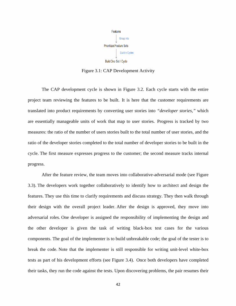
42

Figure 3.1: CAP Development Activity

The CAP development cycle is shown in Figure 3.2. Each cycle starts with the entire

project team reviewing the features to be built. It is here that the customer requirements are

translated into product requirements by converting user stories into “developer stories,” which

are essentially manageable units of work that map to user stories. Progress is tracked by two

measures: the ratio of the number of users stories built to the total number of user stories, and the

ratio of the developer stories completed to the total number of developer stories to be built in the

cycle. The first measure expresses progress to the customer; the second measure tracks internal

progress.

After the feature review, the team moves into collaborative-adversarial mode (see Figure

3.3). The developers work together collaboratively to identify how to architect and design the

features. They use this time to clarify requirements and discuss strategy. They then walk through

their design with the overall project leader. After the design is approved, they move into

adversarial roles. One developer is assigned the responsibility of implementing the design and

the other developer is given the task of writing black-box test cases for the various

components. The goal of the implementer is to build unbreakable code; the goal of the tester is to

break the code. Note that the implementer is still responsible for writing unit-level white-box

tests as part of his development efforts (see Figure 3.4). Once both developers have completed

their tasks, they run the code against the tests. Upon discovering problems, the pair resumes their

43

adversarial positions: the tester verifies that the test cases are valid and the implementer repairs

the code and adds a corresponding regression unit test. In some cases, the test cases are not valid

and are, themselves, fixed by the tester.

At the conclusion of the test phase, the team moves to a post mortem step. Here, the

team (including the project manager) reviews the source code and the test cases. The purpose of

the review is to 1) ensure the test cases are comprehensive and 2) identify portions of the code

that are candidates for refactoring and not to find bugs; so the team does not walk through the

code at a statement-by-statement level. This has been found to be so tedious that the participants

quickly become numb to any problems. It is assumed that the majority of defects are caught in

the blackbox functional tests or in the whitebox unit tests. Any gaps in test cases are captured as

additional developer stories; refactoring tasks are done likewise. These developer stories receive

a high enough priority that they are among the first tasks completed in the subsequent software

development cycle.

A new development cycle begins again by following the post mortem step.

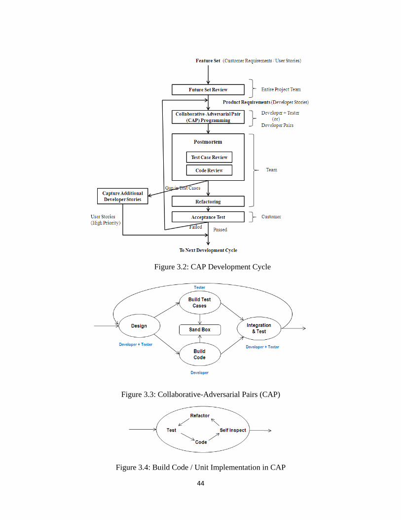
44

Figure 3.2: CAP Development Cycle

Figure 3.3: Collaborative-Adversarial Pairs (CAP)

Figure 3.4: Build Code / Unit Implementation in CAP

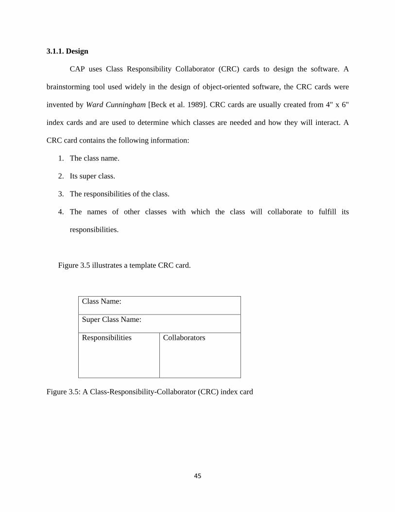
45

3.1.1. Design

CAP uses Class Responsibility Collaborator (CRC) cards to design the software. A

brainstorming tool used widely in the design of object-oriented software, the CRC cards were

invented by Ward Cunningham [Beck et al. 1989]. CRC cards are usually created from 4" x 6"

index cards and are used to determine which classes are needed and how they will interact. A

CRC card contains the following information:

1. The class name.

2. Its super class.

3. The responsibilities of the class.

4. The names of other classes with which the class will collaborate to fulfill its

responsibilities.

Figure 3.5 illustrates a template CRC card.

Class Name:

Super Class Name:

Responsibilities Collaborators

Figure 3.5: A Class-Responsibility-Collaborator (CRC) index card

46

3.1.2. Black Box Test Cases

In functional testing (or behavioral testing), every program is considered to be a function

that maps values from its input domain to values in its output range. The functional testing is also

called black box testing, because testing does not depend on the content or implementation of the

function. Black box testing is completely based on the external specifications (i.e. inputs and

outputs) of the function and is usually data driven.

With functional testing, test cases are developed only from external descriptions of the

software, including specifications, requirements, and design. The functional test cases have the

following two distinct advantages:

1. They are independent from software implementation. Implementation changes do not

affect the test cases and vice-versa.

2. They can be developed in parallel with the implementation, which, in turn, reduces the

overall project development interval.

The functional test cases may suffer from the following two drawbacks:

1. There may be a redundancy in the developed test cases.

2. There can be a probability that portions of the software may be untested.

3.1.3. Unit Implementation

Implementation refers to programming and is intended to satisfy the requirements in the

manner specified by the detailed design. Unit (or software component or module) refers to the

smallest part of the implementation that will be separately maintained. Normally a unit or

software component is a set of collaborating classes. In some cases, a component may contain a

single class. The unit implementation procedure in CAP is given below, which follows the Test-

Driven Development (TDD) approach:

47

1. Write a test unit

2. Compile the test.

• It should fail to compile because the code that the test calls has not been

implemented

3. Implement the methods/write code

• Refactor first if necessary

• Do not compile yet

• Follow the coding standard

• Code in a manner that is easiest to verify

4. Self-inspect the code.

• Do not compile/execute yet

• Be convinced that the code does the required job (the compiler will never do this

because it merely checks the syntax).

• Fill out the code inspection checklist

• Record the time and defect logs

5. Compile the code

• Repair syntax defects

• Record time and defect log

6. Run the test and see it pass.

7. Refactor for clarity and to remove duplication

8. Repeat from the top

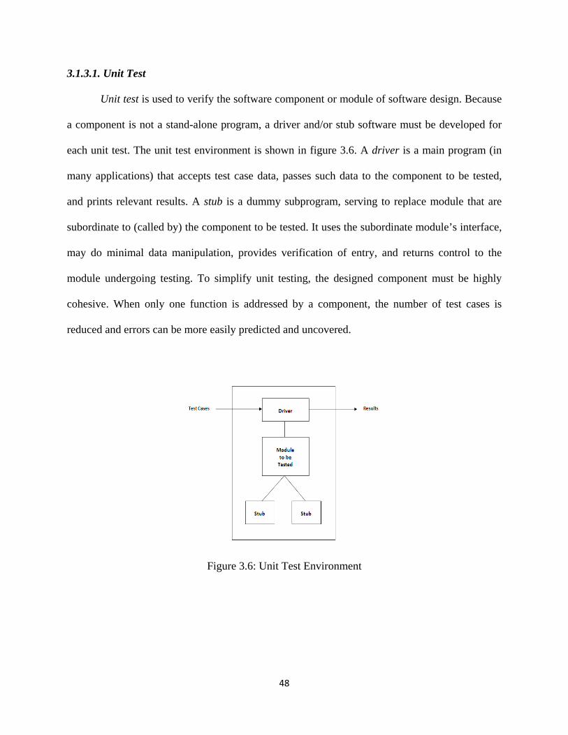
48

3.1.3.1. Unit Test

Unit test is used to verify the software component or module of software design. Because

a component is not a stand-alone program, a driver and/or stub software must be developed for

each unit test. The unit test environment is shown in figure 3.6. A driver is a main program (in

many applications) that accepts test case data, passes such data to the component to be tested,

and prints relevant results. A stub is a dummy subprogram, serving to replace module that are

subordinate to (called by) the component to be tested. It uses the subordinate module’s interface,

may do minimal data manipulation, provides verification of entry, and returns control to the

module undergoing testing. To simplify unit testing, the designed component must be highly

cohesive. When only one function is addressed by a component, the number of test cases is

reduced and errors can be more easily predicted and uncovered.

Figure 3.6: Unit Test Environment

49

3.1.4. Testing in CAP Vs PP

The pair programming methodology uses the white box testing strategy, which has the

following drawbacks:

1. Since the white box test cases are developed from program source code, there is no way

to recognize whether all the specified behaviors are implemented or not.

2. It is very difficult to employ white-box testing on purchased or contracted software

because its internal structure is unknown.

On the other hand, the black box techniques alone are not sufficient enough to identify all

the test cases; indeed, both white box and black box approaches are needed. By combining the

black box and white box testing techniques, we will get the following benefits:

1. The redundancy and gaps problems of black box testing can be recognized and resolved.

2. White box testing aids in identifying behaviors that are not in the specification (such as a

virus). This will never be revealed by black box functional testing.

The CAP testing procedure judiciously combines the functional (black box) and

structural (white box) testing to provide the confidence of functional testing and the

measurement of structural testing.

3.1.5. Refactoring

Refactoring is the process of changing software’s internal structure, in order to improve

design and readability and reduce bugs, without changing its observable behavior. Martin Fowler

[Fowler 1999] suggests that refactoring has to be done in three situations: when adding new

function to the software, when fixing a bug, and when we review the code (i.e., whenever new

idea arises at the time for code review or when the code is identified as being too complex). The

50

first two cases will be covered by the refactoring session of the unit implementation. Since CAP

incorporates the code review session after integration and test, an additional refactoring phase is

necessary. Refactoring also helps developers to review someone else’s code and helps the code

review process to have more concrete results [Fowler 1999].

51

4. APPLIED RESULTS AND RESEARCH VALIDATION

Two empirical experiments were conducted during fall 2008 and spring 2009 to validate

CAP against traditional pair programming and individual programming. The subjects used

Eclipse and JUnit to perform three programming tasks with different degrees of complexity.

4.1. Subjects

Forty two (42) volunteer students from the Software Process class, a combined class of

undergraduate seniors and graduate students, participated in the study. All participants had

already taken software modeling and design (using UML) and computer programming courses

such as C, C++ and Java. Out of fourteen students, 11 students had 1 to 5 years of industrial

programming experience, two had no or less than one year programming experience, and one

student had more than 5 years programming experience. Four students had prior pair

programming experience.

4.2. Experimental Tasks

The subjects were asked to solve the following three programming problems in Java

(Test Driven Development using Eclipse):

Problem1: Write a program which reads a text file and displays the name of the file, the total number of occurrences of a user-input string the total number of non-blank lines in the file, and the count the number of lines of code according to the LOC Counting Standard used in PSP, Personal Software Process [Humphrey 2005]. You may assume that the source code adheres to the LOC Coding Standard. This assignment should not determine if the coding standard has been followed. The program should be capable of sequentially processing multiple files by repeatedly

52

prompting the user for file names until the user enters a file name of "stop". The program should issue the message, "I/O error", if the file is not found or if any other I/O error occurs.

Problem2: Write a program to list information (name, number of methods, type, and

LOC) of each proxy in a source file. The program should also produce an LOC count of the entire source file. Your program should accept as input the name of a file that contains source code. You are to read the file and count the number of lines of code according to our LOC Counting Standard. You may assume that the source code adheres to the LOC Coding Standard. This assignment should not determine if the coding standard has been followed. The exact format of the application-user interaction is up to you.

• A "proxy" is defined as a recognizable software component. Classes are typical proxies in an object-oriented systems; subprograms are typical proxies in traditional functionally-decomposed systems.

• If you are using a functionally-decomposed (meaning, non-OO) approach, the number of methods for each proxy will be "1". If you are using an OO approach, the number of methods will be a count of the methods associated with an object.

Probelm3: Write a program to calculate the planned number of lines of code given the estimated lines of code (using PSP’s PROBE Estimation Script). Your program should accept as input the name of a file. Each line of the file contains four pieces of information separated by a space: the name of a project and its estimated LOC (LOCe), planned LOC (LOCp), and actual LOC (LOCa). Read this file and echo the data to the output device. Accept as input from the keyboard a number which represents the estimated size (E) of a new project. Output the calculations of each decision and the responding planned size (P), as well as the PROBE decision designation (A, B, or C) used to calculate P. For each decision, indicate why it is/isn't valid. The exact format of the application-user interaction is up to you.

• Your software should gracefully handle error conditions, such as non-existent files and invalid input values.

• Round P up to the nearest multiple of 10.

4.3. Hypotheses

H01 (Time/CostOverall): The overall software development cost of CAP is equal or higher

than PP in average.

Ha1 (Time/CostOverall): The overall software development cost of CAP is less than PP in

average.

H02 (Time/CostOverall): The overall software development cost of CAP is equal or higher

than individual programming in average.

53

Ha2 (Time/CostOverall): The overall software development cost of CAP is less than

individual programming in average.

H03 (Time/CostCoding): The cost of CAP coding phase is equal or higher than the cost of

PP coding phase in average.

Ha3 (Time/CostCoding): The cost of CAP coding phase is less than cost of PP coding

phase in average.

H04 (Time/CostCoding): The cost of CAP coding phase is equal or higher than the cost of

individual programming coding phase in average.

Ha4 (Time/CostCoding): The cost of CAP coding phase is less than cost of individual

programming coding phase in average.

H05 (Correctness): The number acceptance tests failed in CAP is equal or higher than

the number of acceptance tests failed in PP in average.

Ha5 (Correctness): The number acceptance tests failed in CAP is less than the number of

acceptance tests failed in PP in average.

4.4. Cost

To study the cost of overall software development, we compared the total development

time, measured in minutes, of all the phases. Both pair programming (PP) and individual

programming (IP) consisted of design, coding and test phases; whereas, the CAP consisted of

test case development phase in addition to the PP phases. The IP, PP and CAP total software

development costs were calculated as per the following formulas:

= TimeDesign + TimeCoding + TimeTest

= 2* (TimeDesign + TimeCoding + TimeTest)

= 2* (TimeDesign + TimeTest) + TimeCoding + TimeTestCaseDevelopment

54

To study the cost of coding phase, we compared the coding time, measured in minutes, of

the coding phase. The IP, PP and CAP coding phase costs were calculated as per the following

formulas.

= TimeCoding

= 2* (TimeCoding)

= TimeCoding

4.5. Program Correctness

To study the program correctness, the number of post-development test cases, black-box

test cases developed from the specifications, passed by programs developed by IP group, PP

group and CAP group were compared.

4.6. Experiment Procedure

1. Consent Process: At the beginning of the course both in fall 2008 and in spring 2009 the

IRB (Auburn University Institutional Review Board) approved informed consent for the

project was handed out and students were given the chance to volunteer to participate.

The researcher provided information to students about the project, handed out consent

forms, answered any questions students raised by the students, and requested that the

forms be returned the following class; so students had at least one intervening day to

review all aspects of consent. The researcher returned the following class and answered

the questions, if any, and collected the consent forms.

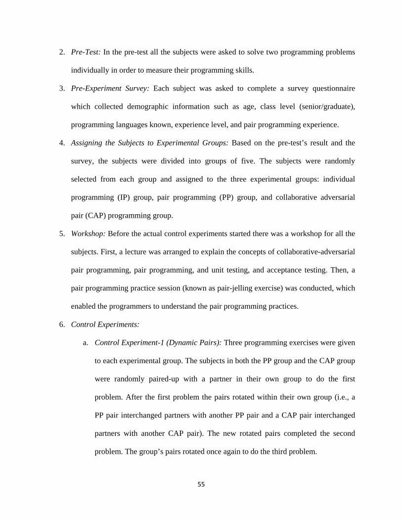
55

2. Pre-Test: In the pre-test all the subjects were asked to solve two programming problems

individually in order to measure their programming skills.

3. Pre-Experiment Survey: Each subject was asked to complete a survey questionnaire

which collected demographic information such as age, class level (senior/graduate),

programming languages known, experience level, and pair programming experience.

4. Assigning the Subjects to Experimental Groups: Based on the pre-test’s result and the

survey, the subjects were divided into groups of five. The subjects were randomly

selected from each group and assigned to the three experimental groups: individual

programming (IP) group, pair programming (PP) group, and collaborative adversarial

pair (CAP) programming group.

5. Workshop: Before the actual control experiments started there was a workshop for all the

subjects. First, a lecture was arranged to explain the concepts of collaborative-adversarial

pair programming, pair programming, and unit testing, and acceptance testing. Then, a

pair programming practice session (known as pair-jelling exercise) was conducted, which

enabled the programmers to understand the pair programming practices.

6. Control Experiments:

a. Control Experiment-1 (Dynamic Pairs): Three programming exercises were given

to each experimental group. The subjects in both the PP group and the CAP group

were randomly paired-up with a partner in their own group to do the first

problem. After the first problem the pairs rotated within their own group (i.e., a

PP pair interchanged partners with another PP pair and a CAP pair interchanged

partners with another CAP pair). The new rotated pairs completed the second

problem. The group’s pairs rotated once again to do the third problem.

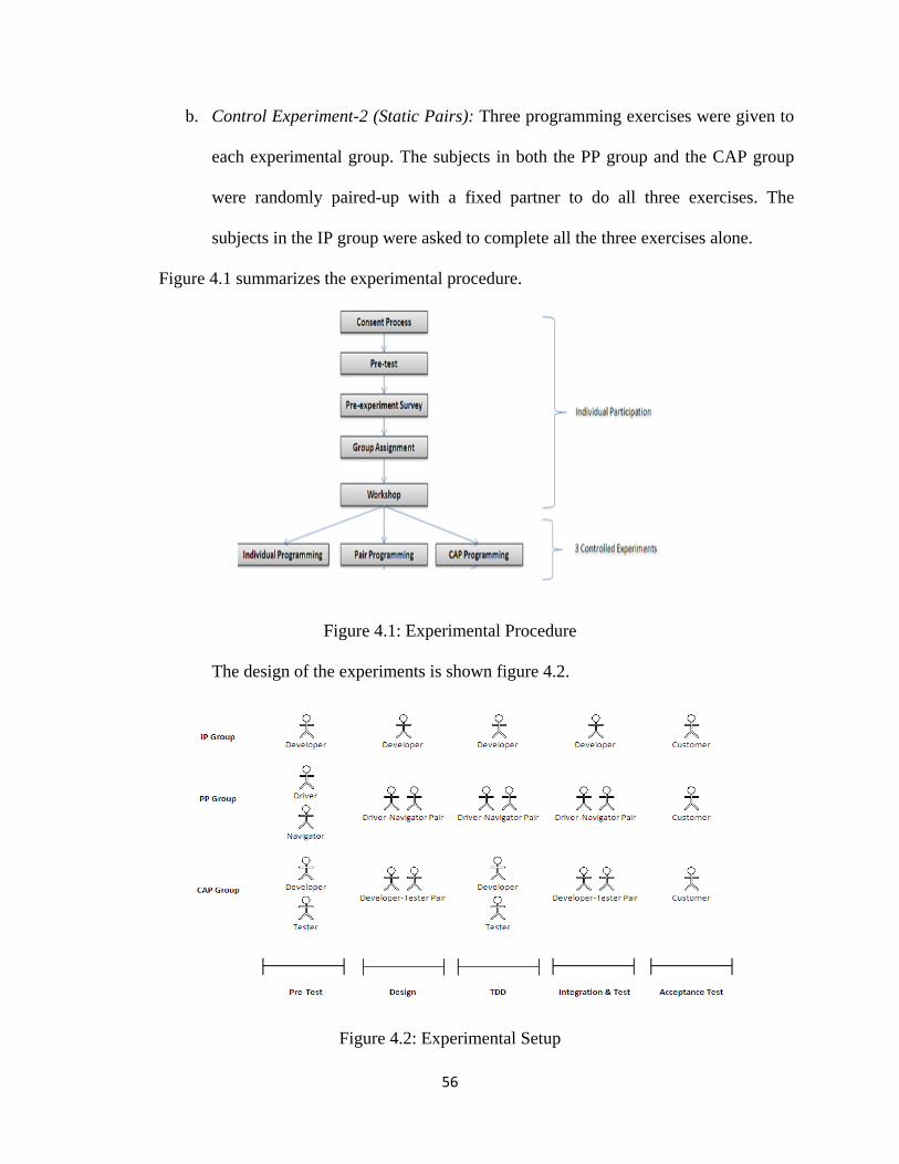
56

b. Control Experiment-2 (Static Pairs): Three programming exercises were given to

each experimental group. The subjects in both the PP group and the CAP group

were randomly paired-up with a fixed partner to do all three exercises. The

subjects in the IP group were asked to complete all the three exercises alone.

Figure 4.1 summarizes the experimental procedure.

Figure 4.1: Experimental Procedure

The design of the experiments is shown figure 4.2.

Figure 4.2: Experimental Setup

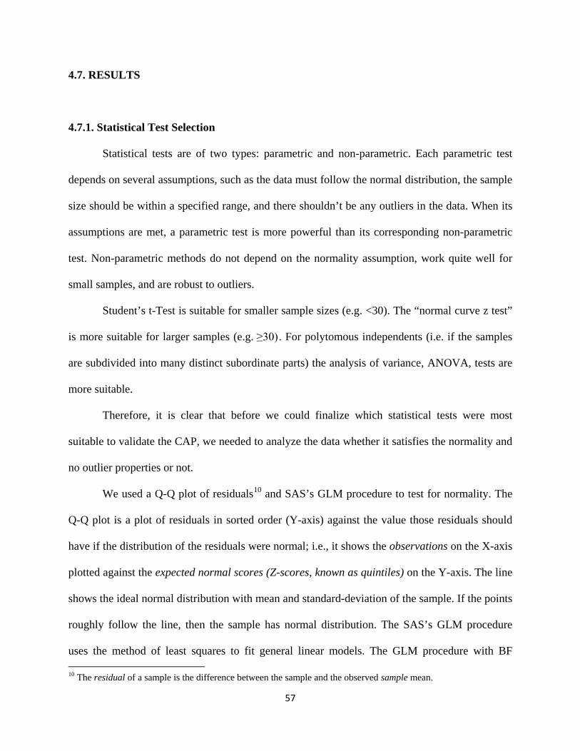
57

4.7. RESULTS

4.7.1. Statistical Test Selection

Statistical tests are of two types: parametric and non-parametric. Each parametric test

depends on several assumptions, such as the data must follow the normal distribution, the sample

size should be within a specified range, and there shouldn’t be any outliers in the data. When its

assumptions are met, a parametric test is more powerful than its corresponding non-parametric

test. Non-parametric methods do not depend on the normality assumption, work quite well for

small samples, and are robust to outliers.

Student’s t-Test is suitable for smaller sample sizes (e.g. <30). The “normal curve z test”

is more suitable for larger samples (e.g. ≥30). For polytomous independents (i.e. if the samples

are subdivided into many distinct subordinate parts) the analysis of variance, ANOVA, tests are

more suitable.

Therefore, it is clear that before we could finalize which statistical tests were most

suitable to validate the CAP, we needed to analyze the data whether it satisfies the normality and

no outlier properties or not.

We used a Q-Q plot of residuals10 and SAS’s GLM procedure to test for normality. The

Q-Q plot is a plot of residuals in sorted order (Y-axis) against the value those residuals should

have if the distribution of the residuals were normal; i.e., it shows the observations on the X-axis

plotted against the expected normal scores (Z-scores, known as quintiles) on the Y-axis. The line

shows the ideal normal distribution with mean and standard-deviation of the sample. If the points

roughly follow the line, then the sample has normal distribution. The SAS’s GLM procedure

uses the method of least squares to fit general linear models. The GLM procedure with BF 10 The residual of a sample is the difference between the sample and the observed sample mean.

58

(Brown and Forsythe’s variation of Levene’s test) option allows us to test the normality of the

sample.

We used a box plot to identify outliers, i.e., data points which are numerically distant

from the rest of the data. In a box plot the outliers are indicated using circles.

4.7.2. Empirical Experiment-1 (Dynamic Pairs-Fall 2008) Test Results

4.7.2.1. Test for Normality

Figures 4.3 and 4.4 show the Q-Q plot of residuals for the total software development

time and coding time, respectively. The points on the Q-Q plots of residuals lie nearly on the

straight line, which indicates that both the total software development time and the coding time

data follows normal distribution.

Figure 4.3: Q-Q Plot of Residuals (Dynamic Pairs Total Software Development Time)

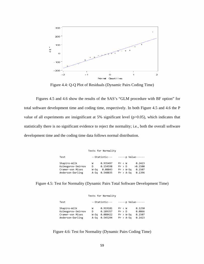
59

Figure 4.4: Q-Q Plot of Residuals (Dynamic Pairs Coding Time)

Figures 4.5 and 4.6 show the results of the SAS’s “GLM procedure with BF option” for

total software development time and coding time, respectively. In both Figure 4.5 and 4.6 the P

value of all experiments are insignificant at 5% significant level (p>0.05), which indicates that

statistically there is no significant evidence to reject the normality; i.e., both the overall software

development time and the coding time data follows normal distribution.

Tests for Normality

Test --Statistic--- -----p Value------

Shapiro-Wilk W 0.935497 Pr < W 0.2423 Kolmogorov-Smirnov D 0.154598 Pr > D >0.1500 Cramer-von Mises W-Sq 0.08843 Pr > W-Sq 0.1507 Anderson-Darling A-Sq 0.548835 Pr > A-Sq 0.1396

Figure 4.5: Test for Normality (Dynamic Pairs Total Software Development Time)

Tests for Normality


Shapiro-Wilk W 0.919181 Pr < W 0.1250 Kolmogorov-Smirnov D 0.189357 Pr > D 0.0866 Cramer-von Mises W-Sq 0.088422 Pr > W-Sq 0.1507 Anderson-Darling A-Sq 0.545294 Pr > A-Sq 0.1423

Figure 4.6: Test for Normality (Dynamic Pairs Coding Time)

60

4.7.2.2. Outliers

The box plots for the total software development time and coding time are given in

Figures 4.7 and 4.8 respectively. There are no circles in Figures 4.7 and 4.8, which indicates that

there are no outliers either in PP’s overall software development time and coding time or in

CAP’s overall software development time and coding time.

Figure 4.7: Box plot (Dynamic Pairs Total Software Development Time)

Figure 4.8: Box plot (Dynamic Pairs Coding Time)

CAP PP

100

200

300

400

500

600

ttime

indicator

CAP PP

0

100

200

300

400

500

ctime

indicator

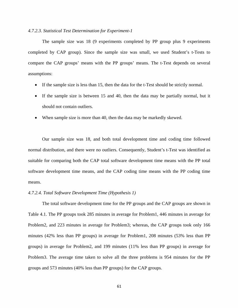
61

4.7.2.3. Statistical Test Determination for Experiment-1

The sample size was 18 (9 experiments completed by PP group plus 9 experiments

completed by CAP group). Since the sample size was small, we used Student’s t-Tests to

compare the CAP groups’ means with the PP groups’ means. The t-Test depends on several

assumptions:

• If the sample size is less than 15, then the data for the t-Test should be strictly normal.

• If the sample size is between 15 and 40, then the data may be partially normal, but it

should not contain outliers.

• When sample size is more than 40, then the data may be markedly skewed.

Our sample size was 18, and both total development time and coding time followed

normal distribution, and there were no outliers. Consequently, Student’s t-Test was identified as

suitable for comparing both the CAP total software development time means with the PP total

software development time means, and the CAP coding time means with the PP coding time

means.

4.7.2.4. Total Software Development Time (Hypothesis 1)

The total software development time for the PP groups and the CAP groups are shown in

Table 4.1. The PP groups took 285 minutes in average for Problem1, 446 minutes in average for

Problem2, and 223 minutes in average for Problem3; whereas, the CAP groups took only 166

minutes (42% less than PP groups) in average for Problem1, 208 minutes (53% less than PP

groups) in average for Problem2, and 199 minutes (11% less than PP groups) in average for

Problem3. The average time taken to solve all the three problems is 954 minutes for the PP

groups and 573 minutes (40% less than PP groups) for the CAP groups.

62

Method Problem1 Problem2 Problem3 CAP-G1 180 275 120 CAP-G2 148 189 273 CAP-G3 171 160 204 Average 166 208 199 PP-G1 250 488 272 PP-G2 342 346 256 PP-G3 264 504 140

Average 285 446 223 Table 4.1: Total Software Development Time (Dynamic Pairs)

Figure 4.9 shows the average time taken by PP groups and CAP groups for the total

software development for the given three problems.

Figure 4.9: Average Total Software Development Time (Dynamic Pairs)

The box plot in Figure 4.10 shows the total time taken by all 18 pairs (3x3 programs

completed by PP groups and 3x3 programs completed by CAP groups). The boxes contain 50%

of the data points, the line between lower border and box contain 25% of data points, and the line

between the box and upper border contain another 25% data points. The plus mark in the plot

(box) indicates the mean value and the horizontal line in the middle of the box indicates the

median value. The plot indicates that all the nine CAP programs took less time than the mean

value of the PP programs.

166 208 199285

446

223

0100200300400500

P1 P2 P3

CAP

PP

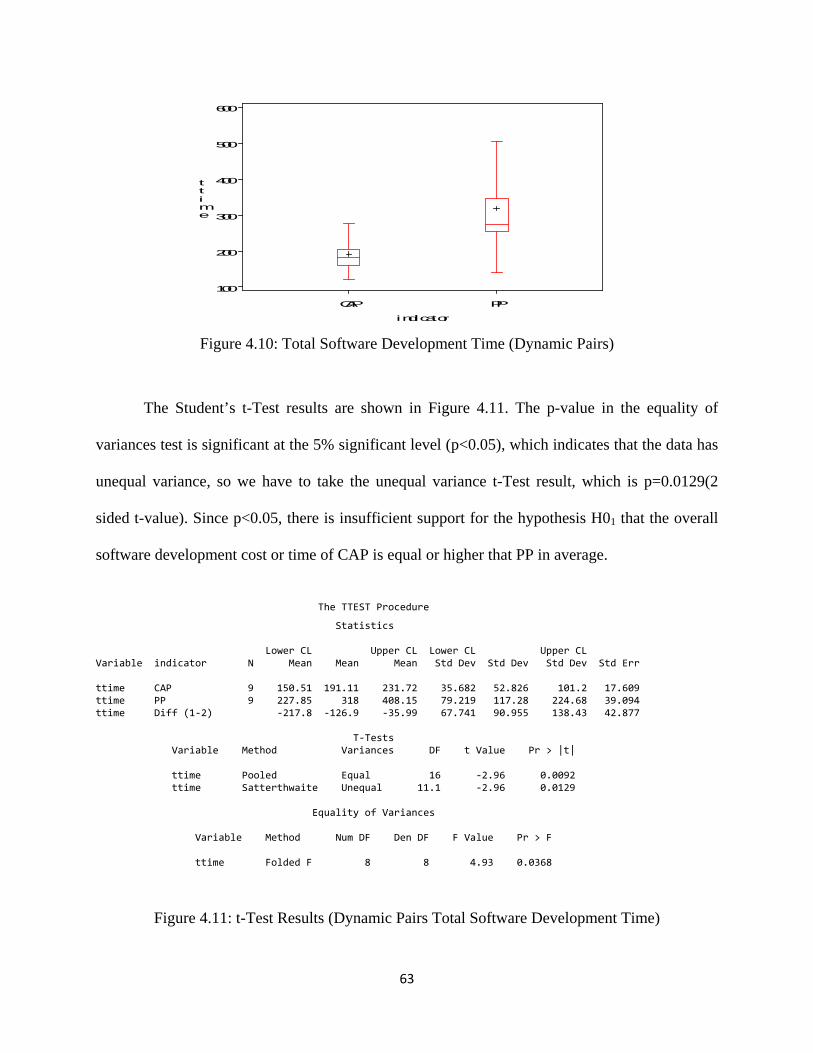
63

Figure 4.10: Total Software Development Time (Dynamic Pairs)

The Student’s t-Test results are shown in Figure 4.11. The p-value in the equality of

variances test is significant at the 5% significant level (p<0.05), which indicates that the data has

unequal variance, so we have to take the unequal variance t-Test result, which is p=0.0129(2

sided t-value). Since p<0.05, there is insufficient support for the hypothesis H01 that the overall

software development cost or time of CAP is equal or higher that PP in average.

The TTEST Procedure

Statistics Lower CL Upper CL Lower CL Upper CL Variable indicator N Mean Mean Mean Std Dev Std Dev Std Dev Std Err ttime CAP 9 150.51 191.11 231.72 35.682 52.826 101.2 17.609 ttime PP 9 227.85 318 408.15 79.219 117.28 224.68 39.094 ttime Diff (1-2) -217.8 -126.9 -35.99 67.741 90.955 138.43 42.877 T-Tests Variable Method Variances DF t Value Pr > |t| ttime Pooled Equal 16 -2.96 0.0092 ttime Satterthwaite Unequal 11.1 -2.96 0.0129 Equality of Variances Variable Method Num DF Den DF F Value Pr > F ttime Folded F 8 8 4.93 0.0368

Figure 4.11: t-Test Results (Dynamic Pairs Total Software Development Time)

CAP PP

100

200

300

400

500

600

ttime

indicator

64

Decision: Reject H01 in favor of Ha1 since p-value < α (α=0.05). Thus we have sufficient

statistical evidence to conclude that the overall software development cost or time of CAP is less

than PP in average.

4.7.2.5. Coding Time (Hypothesis 3)

The coding time for the PP groups and the CAP groups are shown in Table 4.2. The PP

groups took 192 minutes in average for Problem1, 371 minutes in average for Problem2, and 170

minutes in average for Problem3; whereas, the CAP groups took only 65 minutes (66% less than

PP groups) in average for Problem1, 52 minutes (86% less than PP groups) in average for

Problem2, and 79 minutes (54% less than PP groups) in average for Problem3. The average time

taken to solve all the three problems is 733 minutes for PP groups and 196 minutes (73% less

than PP groups) for CAP groups.


Average 192 371 170 Table 4.2: Coding Time (Dynamic Pairs)

Figure 4.12 shows the average time taken by PP groups and CAP groups for the coding

phase of the software development for the given three problems.

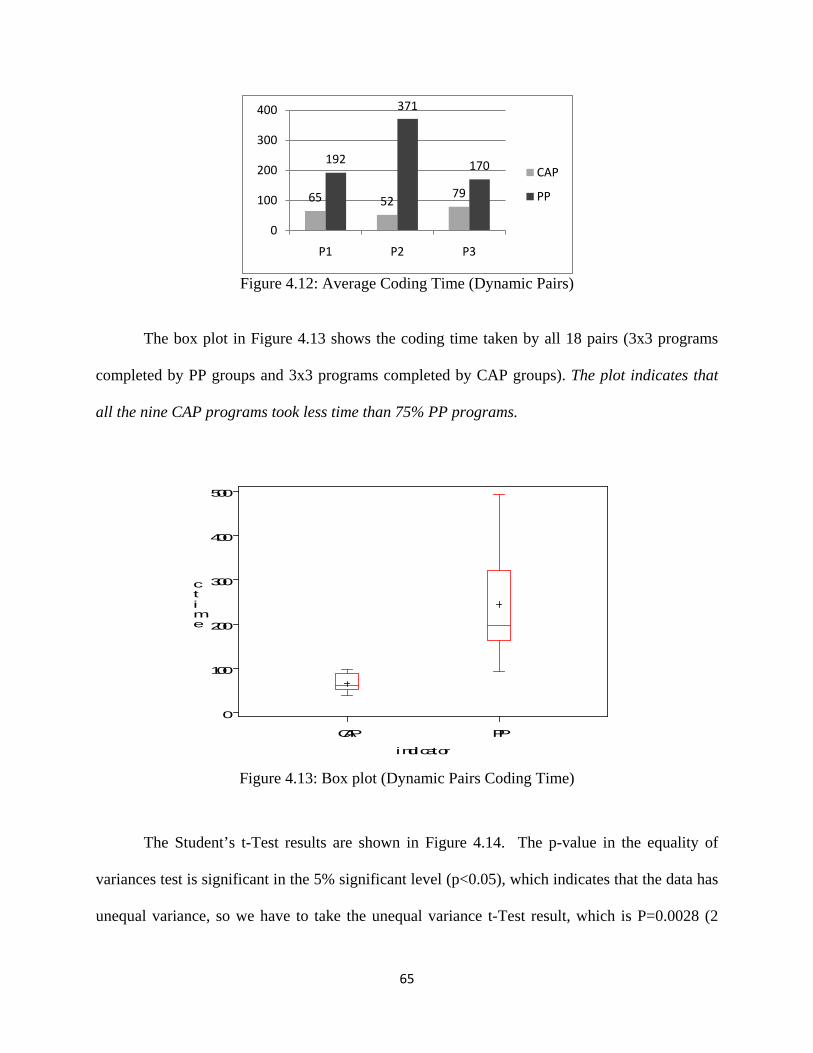
65

Figure 4.12: Average Coding Time (Dynamic Pairs)

The box plot in Figure 4.13 shows the coding time taken by all 18 pairs (3x3 programs

completed by PP groups and 3x3 programs completed by CAP groups). The plot indicates that

all the nine CAP programs took less time than 75% PP programs.

Figure 4.13: Box plot (Dynamic Pairs Coding Time)


variances test is significant in the 5% significant level (p<0.05), which indicates that the data has

unequal variance, so we have to take the unequal variance t-Test result, which is P=0.0028 (2

65 5279

192

371

170

0

100

200

300

400

P1 P2 P3

CAP

PP

CAP PP

0

100

200

300

400

500

ctime

indicator

66

sided t-value). Since P<0.05, there is insufficient support for the hypothesis H03 that the cost of

the CAP coding phase is equal or higher that PP coding phase in average.

The TTEST Procedure Statistics Lower CL Upper CL Lower CL Upper CL Variable indicator N Mean Mean Mean Std Dev Std Dev Std Dev Std Err ctime CAP 9 48.133 65.333 82.534 15.115 22.377 42.87 7.4591 ctime PP 9 146.56 244.22 341.89 85.821 127.06 243.41 42.352 ctime Diff (1-2) -270.1 -178.9 -87.72 67.942 91.226 138.84 43.004 T-Tests Variable Method Variances DF t Value Pr > |t| ctime Pooled Equal 16 -4.16 0.0007 ctime Satterthwaite Unequal 8.5 -4.16 0.0028 Equality of Variances Variable Method Num DF Den DF F Value Pr > F ctime Folded F 8 8 32.24 <.0001

Figure 4.14: t-Test Results (Dynamic Pairs Coding Time)


statistical evidence to conclude that the cost of CAP coding phase is less than the cost of PP

coding phase in average.

4.7.2.6. Program Correctness (Hypothesis 5)

The number of post-development test cases passed by the PP group programs and the

CAP group programs are shown in Table 4.3 and Figure 4.15. The acceptance tests were

conducted by a disinterested party. Specifically, a graduate teaching assistant for the introductory

Java course was recruited to do this. The tester was not involved in any other way with the

experiment. The total numbers of test cases passed by the PP groups was 13, 17, and 29 for

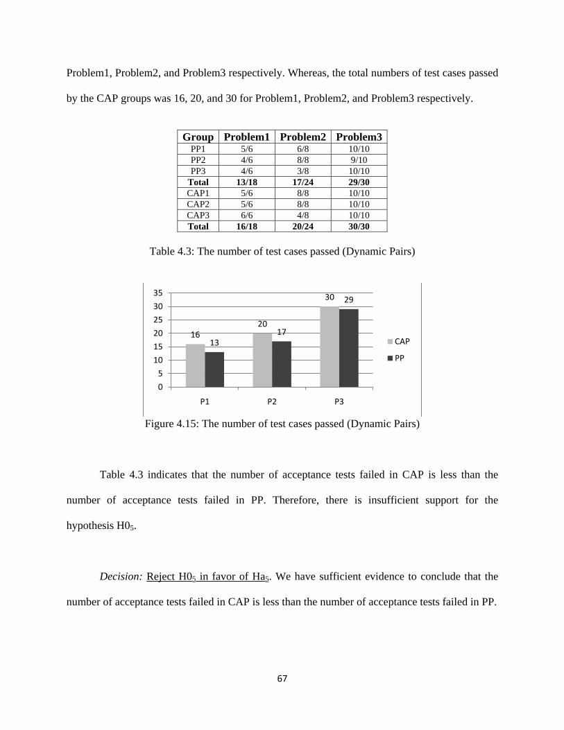
67

Problem1, Problem2, and Problem3 respectively. Whereas, the total numbers of test cases passed

by the CAP groups was 16, 20, and 30 for Problem1, Problem2, and Problem3 respectively.

Group Problem1 Problem2 Problem3

PP1 5/6 6/8 10/10 PP2 4/6 8/8 9/10 PP3 4/6 3/8 10/10

Total 13/18 17/24 29/30 CAP1 5/6 8/8 10/10 CAP2 5/6 8/8 10/10 CAP3 6/6 4/8 10/10 Total 16/18 20/24 30/30

Table 4.3: The number of test cases passed (Dynamic Pairs)

Figure 4.15: The number of test cases passed (Dynamic Pairs)

Table 4.3 indicates that the number of acceptance tests failed in CAP is less than the

number of acceptance tests failed in PP. Therefore, there is insufficient support for the

hypothesis H05.

Decision: Reject H05 in favor of Ha5. We have sufficient evidence to conclude that the

number of acceptance tests failed in CAP is less than the number of acceptance tests failed in PP.

1620

30

1317

29

0

5

10

15

20

25

30

35

P1 P2 P3

CAP

PP

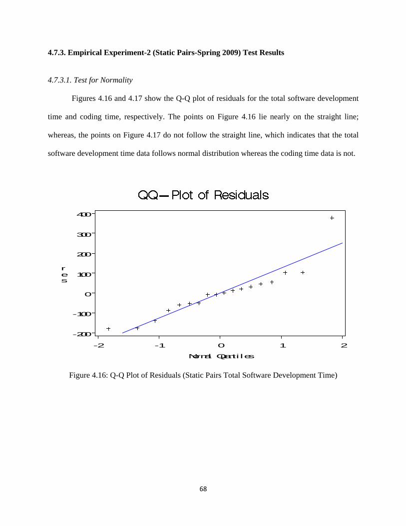
68

4.7.3. Empirical Experiment-2 (Static Pairs-Spring 2009) Test Results



time and coding time, respectively. The points on Figure 4.16 lie nearly on the straight line;

whereas, the points on Figure 4.17 do not follow the straight line, which indicates that the total

software development time data follows normal distribution whereas the coding time data is not.

Figure 4.16: Q-Q Plot of Residuals (Static Pairs Total Software Development Time)

-2 -1 0 1 2

-200

-100

0

100

200

300

400

res

Normal Quanti les

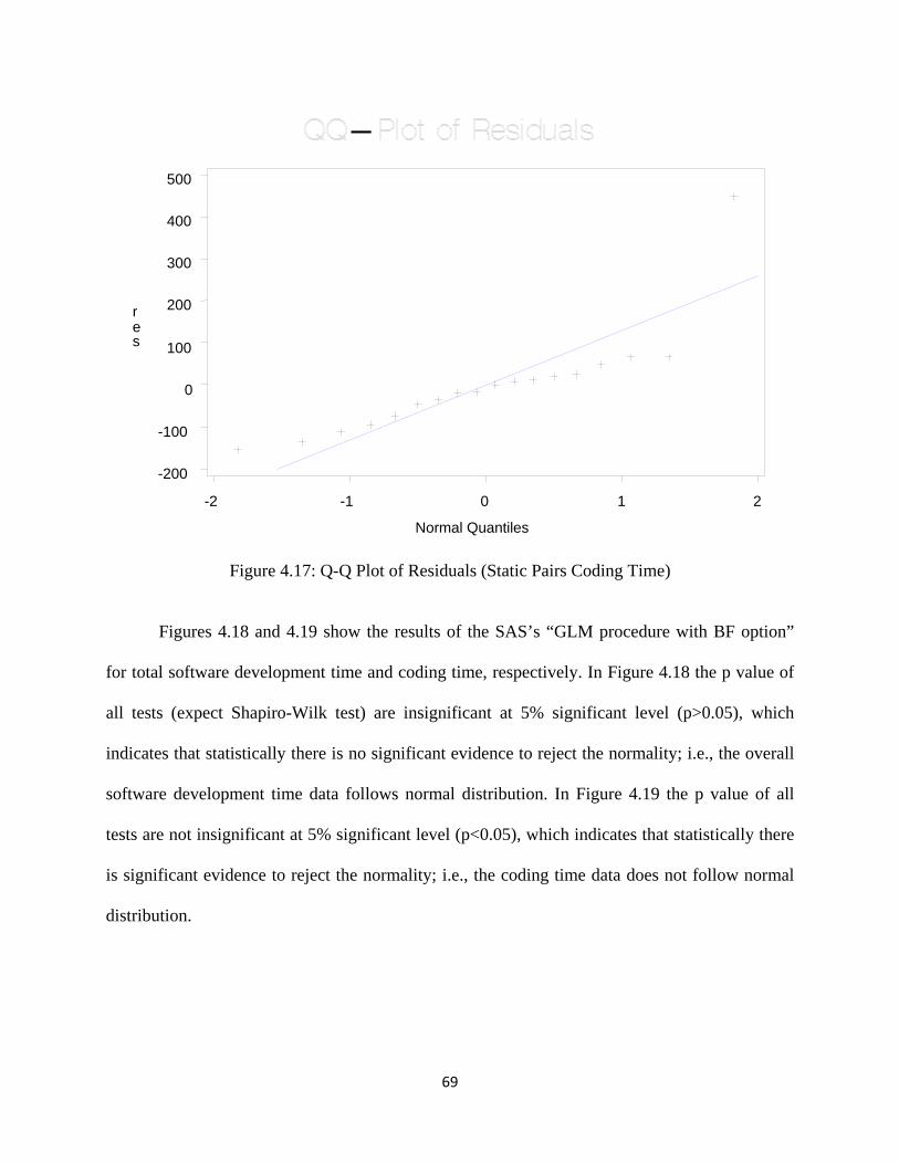
69

Figure 4.17: Q-Q Plot of Residuals (Static Pairs Coding Time)

Figures 4.18 and 4.19 show the results of the SAS’s “GLM procedure with BF option”

for total software development time and coding time, respectively. In Figure 4.18 the p value of

all tests (expect Shapiro-Wilk test) are insignificant at 5% significant level (p>0.05), which

indicates that statistically there is no significant evidence to reject the normality; i.e., the overall

software development time data follows normal distribution. In Figure 4.19 the p value of all

tests are not insignificant at 5% significant level (p<0.05), which indicates that statistically there

is significant evidence to reject the normality; i.e., the coding time data does not follow normal

distribution.

-2 -1 0 1 2

-200

-100

0

100

200

300

400

500

r e s

Normal Quantiles

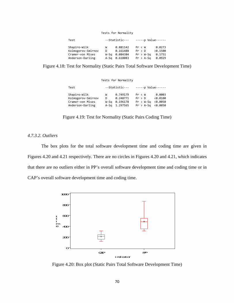
70

Tests for Normality



Figure 4.18: Test for Normality (Static Pairs Total Software Development Time)

Tests for Normality


Shapiro-Wilk W 0.749179 Pr < W 0.0003 Kolmogorov-Smirnov D 0.248771 Pr > D <0.0100 Cramer-von Mises W-Sq 0.196178 Pr > W-Sq <0.0050 Anderson-Darling A-Sq 1.297565 Pr > A-Sq <0.0050

Figure 4.19: Test for Normality (Static Pairs Coding Time)

4.7.3.2. Outliers


Figures 4.20 and 4.21 respectively. There are no circles in Figures 4.20 and 4.21, which indicates

that there are no outliers either in PP’s overall software development time and coding time or in


Figure 4.20: Box plot (Static Pairs Total Software Development Time)

CAP PP

0

200

400

600

800

1000

ttime

indicator

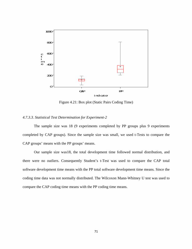
71

Figure 4.21: Box plot (Static Pairs Coding Time)

4.7.3.3. Statistical Test Determination for Experiment-2

The sample size was 18 (9 experiments completed by PP groups plus 9 experiments

completed by CAP groups). Since the sample size was small, we used t-Tests to compare the

CAP groups’ means with the PP groups’ means.

Our sample size was18, the total development time followed normal distribution, and

there were no outliers. Consequently Student’s t-Test was used to compare the CAP total

software development time means with the PP total software development time means. Since the

coding time data was not normally distributed. The Wilcoxon Mann-Whitney U test was used to

compare the CAP coding time means with the PP coding time means.

CAP PP

0

200

400

600

800

1000

ctime

indicator

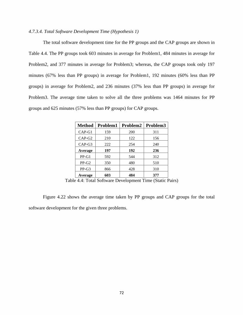
72


The total software development time for the PP groups and the CAP groups are shown in

Table 4.4. The PP groups took 603 minutes in average for Problem1, 484 minutes in average for




Problem3. The average time taken to solve all the three problems was 1464 minutes for PP

groups and 625 minutes (57% less than PP groups) for CAP groups.


Average 603 484 377 Table 4.4: Total Software Development Time (Static Pairs)



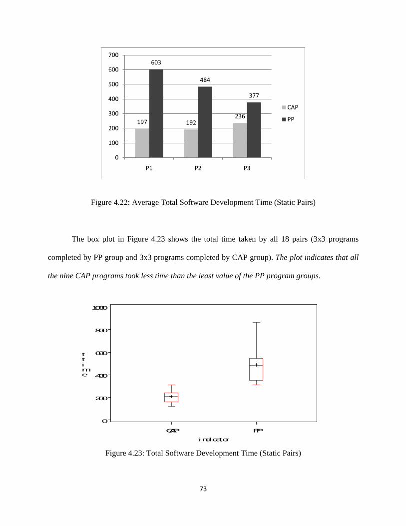
73

Figure 4.22: Average Total Software Development Time (Static Pairs)


completed by PP group and 3x3 programs completed by CAP group). The plot indicates that all

the nine CAP programs took less time than the least value of the PP program groups.

Figure 4.23: Total Software Development Time (Static Pairs)

197 192236

603

484

377

0

100

200

300

400

500

600

700

P1 P2 P3

CAP

PP

CAP PP

0

200

400

600

800

1000

ttime

indicator

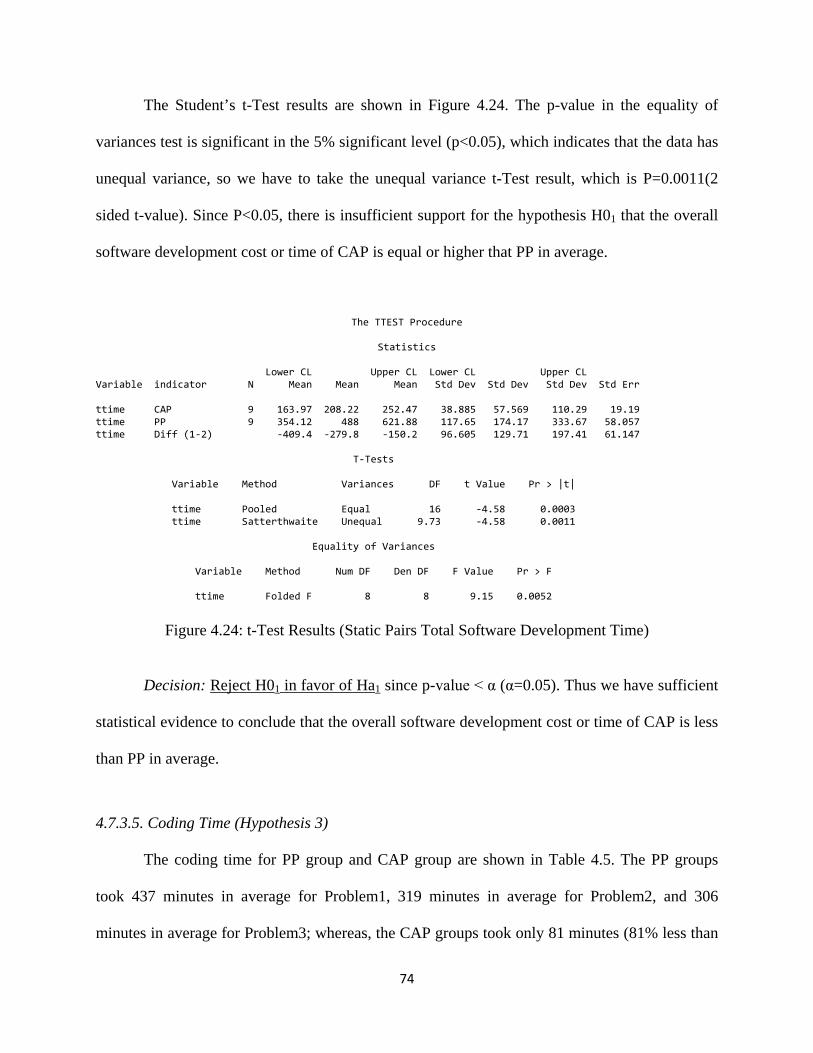
74


variances test is significant in the 5% significant level (p<0.05), which indicates that the data has

unequal variance, so we have to take the unequal variance t-Test result, which is P=0.0011(2

sided t-value). Since P<0.05, there is insufficient support for the hypothesis H01 that the overall


The TTEST Procedure

Statistics Lower CL Upper CL Lower CL Upper CL Variable indicator N Mean Mean Mean Std Dev Std Dev Std Dev Std Err ttime CAP 9 163.97 208.22 252.47 38.885 57.569 110.29 19.19 ttime PP 9 354.12 488 621.88 117.65 174.17 333.67 58.057 ttime Diff (1-2) -409.4 -279.8 -150.2 96.605 129.71 197.41 61.147 T-Tests Variable Method Variances DF t Value Pr > |t| ttime Pooled Equal 16 -4.58 0.0003 ttime Satterthwaite Unequal 9.73 -4.58 0.0011 Equality of Variances Variable Method Num DF Den DF F Value Pr > F ttime Folded F 8 8 9.15 0.0052

Figure 4.24: t-Test Results (Static Pairs Total Software Development Time)



than PP in average.


The coding time for PP group and CAP group are shown in Table 4.5. The PP groups

took 437 minutes in average for Problem1, 319 minutes in average for Problem2, and 306


75


Problem2, and 142 minutes (54% less than PP groups) in average for Problem3. The average

time taken to solve all the three problems was 1062 minutes for PP groups and 340 minutes

(68% less than PP groups) for CAP groups.


Average 437 319 306 Table 4.5: Coding Time (Static Pairs)



Figure 4.25: Average Coding Time (Static Pairs)

81117

142

437

319 306

050

100150200250300350400450500

P1 P2 P3

CAP

PP

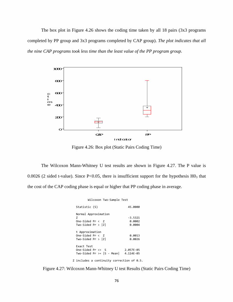
76



the nine CAP programs took less time than the least value of the PP program group.

Figure 4.26: Box plot (Static Pairs Coding Time)

The Wilcoxon Mann-Whitney U test results are shown in Figure 4.27. The P value is

0.0026 (2 sided t-value). Since P<0.05, there is insufficient support for the hypothesis H03 that

the cost of the CAP coding phase is equal or higher that PP coding phase in average.

Wilcoxon Two-Sample Test Statistic (S) 45.0000 Normal Approximation Z -3.5321 One-Sided Pr < Z 0.0002 Two-Sided Pr > |Z| 0.0004 t Approximation One-Sided Pr < Z 0.0013 Two-Sided Pr > |Z| 0.0026 Exact Test One-Sided Pr <= S 2.057E-05 Two-Sided Pr >= |S - Mean| 4.114E-05 Z includes a continuity correction of 0.5.

Figure 4.27: Wilcoxon Mann-Whitney U test Results (Static Pairs Coding Time)

CAP PP

0

200

400

600

800

1000

ctime

indicator

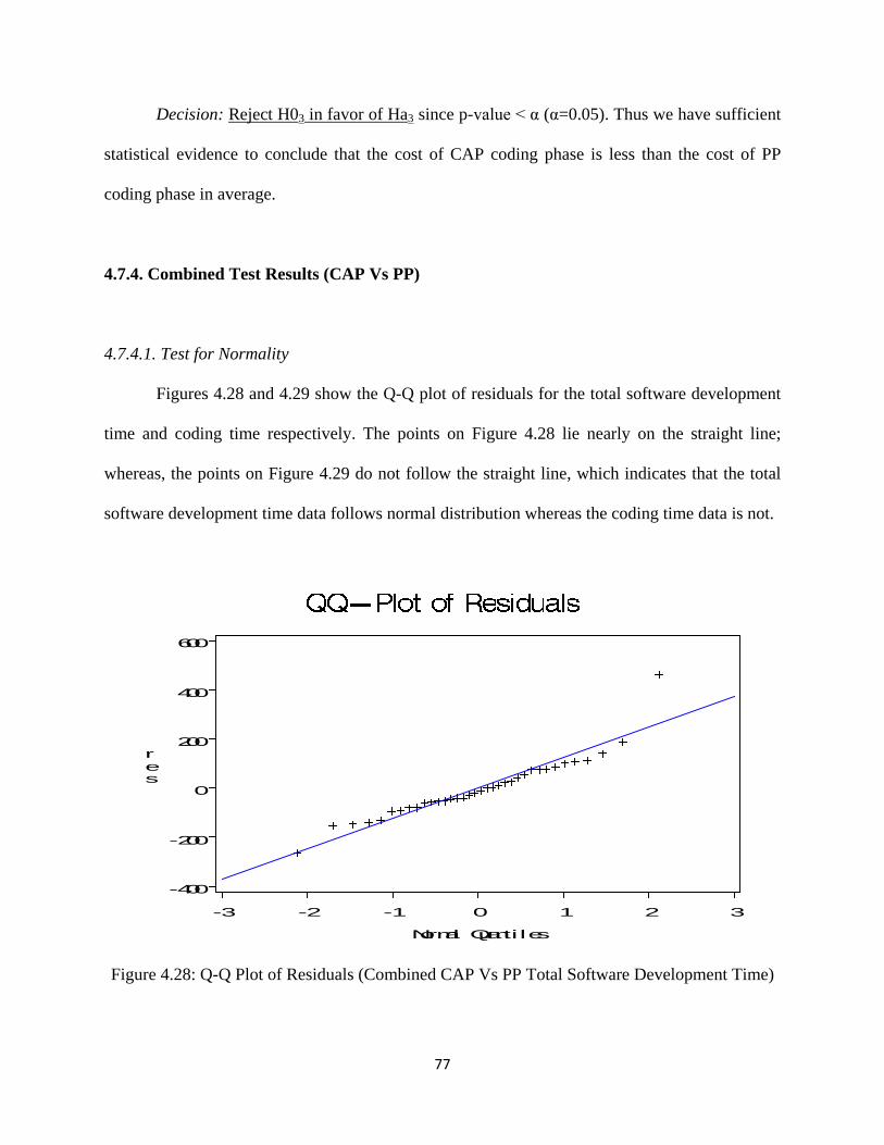
77




4.7.4. Combined Test Results (CAP Vs PP)



time and coding time respectively. The points on Figure 4.28 lie nearly on the straight line;

whereas, the points on Figure 4.29 do not follow the straight line, which indicates that the total

software development time data follows normal distribution whereas the coding time data is not.

Figure 4.28: Q-Q Plot of Residuals (Combined CAP Vs PP Total Software Development Time)

-3 -2 -1 0 1 2 3

-400

-200

0

200

400

600

res

Normal Quanti les

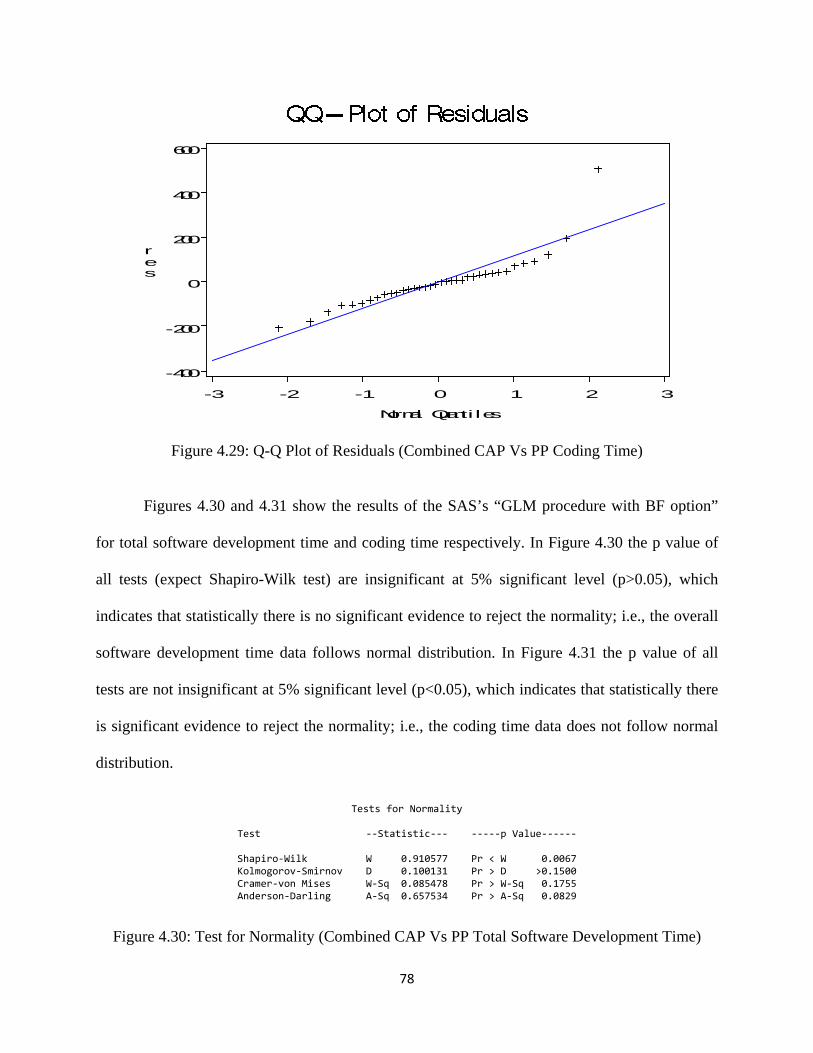
78

Figure 4.29: Q-Q Plot of Residuals (Combined CAP Vs PP Coding Time)


for total software development time and coding time respectively. In Figure 4.30 the p value of

all tests (expect Shapiro-Wilk test) are insignificant at 5% significant level (p>0.05), which

indicates that statistically there is no significant evidence to reject the normality; i.e., the overall

software development time data follows normal distribution. In Figure 4.31 the p value of all

tests are not insignificant at 5% significant level (p<0.05), which indicates that statistically there

is significant evidence to reject the normality; i.e., the coding time data does not follow normal

distribution.

Tests for Normality



Figure 4.30: Test for Normality (Combined CAP Vs PP Total Software Development Time)

-3 -2 -1 0 1 2 3

-400

-200

0

200

400

600

res

Normal Quanti les

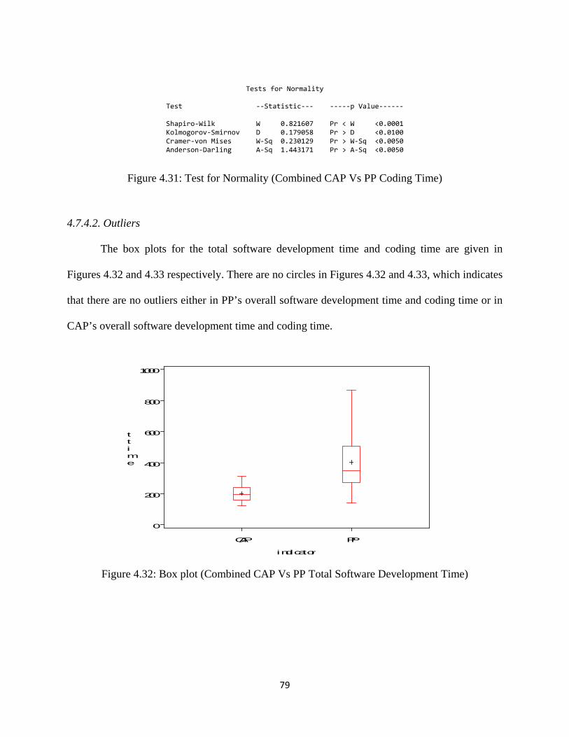
79

Tests for Normality


Shapiro-Wilk W 0.821607 Pr < W <0.0001 Kolmogorov-Smirnov D 0.179058 Pr > D <0.0100 Cramer-von Mises W-Sq 0.230129 Pr > W-Sq <0.0050 Anderson-Darling A-Sq 1.443171 Pr > A-Sq <0.0050

Figure 4.31: Test for Normality (Combined CAP Vs PP Coding Time)

4.7.4.2. Outliers


Figures 4.32 and 4.33 respectively. There are no circles in Figures 4.32 and 4.33, which indicates



Figure 4.32: Box plot (Combined CAP Vs PP Total Software Development Time)

CAP PP

0

200

400

600

800

1000

ttime

indicator

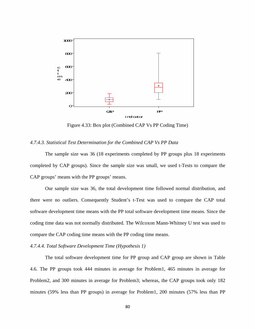
80

Figure 4.33: Box plot (Combined CAP Vs PP Coding Time)

4.7.4.3. Statistical Test Determination for the Combined CAP Vs PP Data

The sample size was 36 (18 experiments completed by PP groups plus 18 experiments

completed by CAP groups). Since the sample size was small, we used t-Tests to compare the

CAP groups’ means with the PP groups’ means.

Our sample size was 36, the total development time followed normal distribution, and

there were no outliers. Consequently Student’s t-Test was used to compare the CAP total

software development time means with the PP total software development time means. Since the

coding time data was not normally distributed. The Wilcoxon Mann-Whitney U test was used to

compare the CAP coding time means with the PP coding time means.


The total software development time for PP group and CAP group are shown in Table

4.6. The PP groups took 444 minutes in average for Problem1, 465 minutes in average for



CAP PP

0

200

400

600

800

1000

ctime

indicator

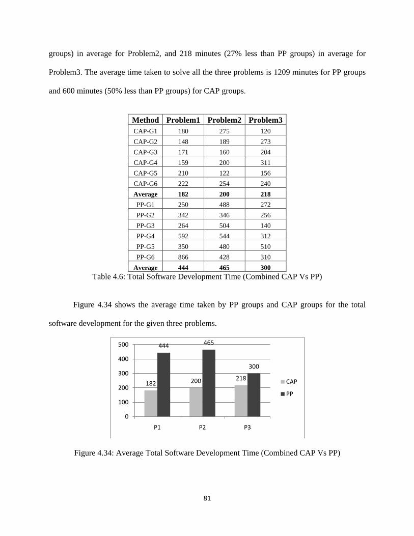
81


Problem3. The average time taken to solve all the three problems is 1209 minutes for PP groups

and 600 minutes (50% less than PP groups) for CAP groups.

Method Problem1 Problem2 Problem3 CAP-G1 180 275 120 CAP-G2 148 189 273 CAP-G3 171 160 204 CAP-G4 159 200 311 CAP-G5 210 122 156 CAP-G6 222 254 240 Average 182 200 218 PP-G1 250 488 272 PP-G2 342 346 256 PP-G3 264 504 140 PP-G4 592 544 312 PP-G5 350 480 510 PP-G6 866 428 310

Average 444 465 300 Table 4.6: Total Software Development Time (Combined CAP Vs PP)



Figure 4.34: Average Total Software Development Time (Combined CAP Vs PP)

182 200 218

444 465

300

0

100

200

300

400

500

P1 P2 P3

CAP

PP

82


completed by PP groups and 6x3 programs completed by CAP groups). The plot indicates that

all the nine CAP programs took less time than the least value of the PP program groups.

Figure 4.35: Box Plot (Combined CAP Vs PP Total Software Development Time)

The Student’s t-Test results are shown in Figure 4.36. The p-value in the equality

of variances test is significant in the 5% significant level (p<0.05), which indicates that the data

has unequal variance, so we have to take the unequal variance t-Test result, which is P<0.0001(2

sided t-value). Since P<0.05, there is insufficient support for the hypothesis H01 that the overall


CAP PP

0

200

400

600

800

1000

ttime

indicator

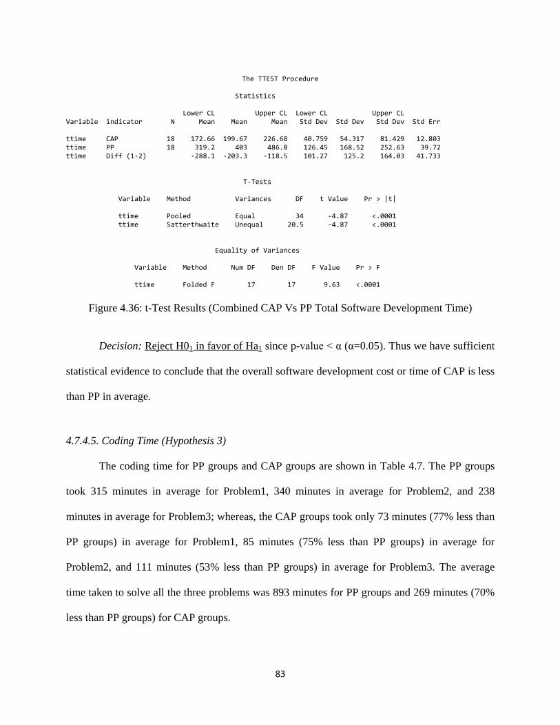
83

The TTEST Procedure

Statistics Lower CL Upper CL Lower CL Upper CL Variable indicator N Mean Mean Mean Std Dev Std Dev Std Dev Std Err ttime CAP 18 172.66 199.67 226.68 40.759 54.317 81.429 12.803 ttime PP 18 319.2 403 486.8 126.45 168.52 252.63 39.72 ttime Diff (1-2) -288.1 -203.3 -118.5 101.27 125.2 164.03 41.733 T-Tests Variable Method Variances DF t Value Pr > |t| ttime Pooled Equal 34 -4.87 <.0001 ttime Satterthwaite Unequal 20.5 -4.87 <.0001 Equality of Variances Variable Method Num DF Den DF F Value Pr > F ttime Folded F 17 17 9.63 <.0001

Figure 4.36: t-Test Results (Combined CAP Vs PP Total Software Development Time)



than PP in average.


The coding time for PP groups and CAP groups are shown in Table 4.7. The PP groups

took 315 minutes in average for Problem1, 340 minutes in average for Problem2, and 238



Problem2, and 111 minutes (53% less than PP groups) in average for Problem3. The average

time taken to solve all the three problems was 893 minutes for PP groups and 269 minutes (70%

less than PP groups) for CAP groups.

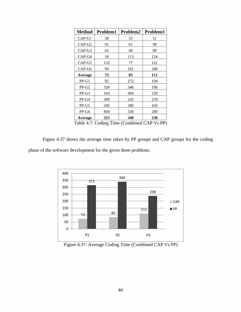
84

Method Problem1 Problem2 Problem3 CAP-G1 38 55 51 CAP-G2 91 61 98 CAP-G3 65 40 89 CAP-G4 18 113 124 CAP-G5 132 77 121 CAP-G6 94 161 180 Average 73 85 111 PP-G1 92 272 194 PP-G2 320 346 196 PP-G3 164 494 120 PP-G4 308 242 218 PP-G5 200 380 420 PP-G6 804 336 280

Average 315 340 238 Table 4.7: Coding Time (Combined CAP Vs PP)



Figure 4.37: Average Coding Time (Combined CAP Vs PP)

73 85111

315340

238

0

50

100

150

200

250

300

350

400

P1 P2 P3

CAP

PP

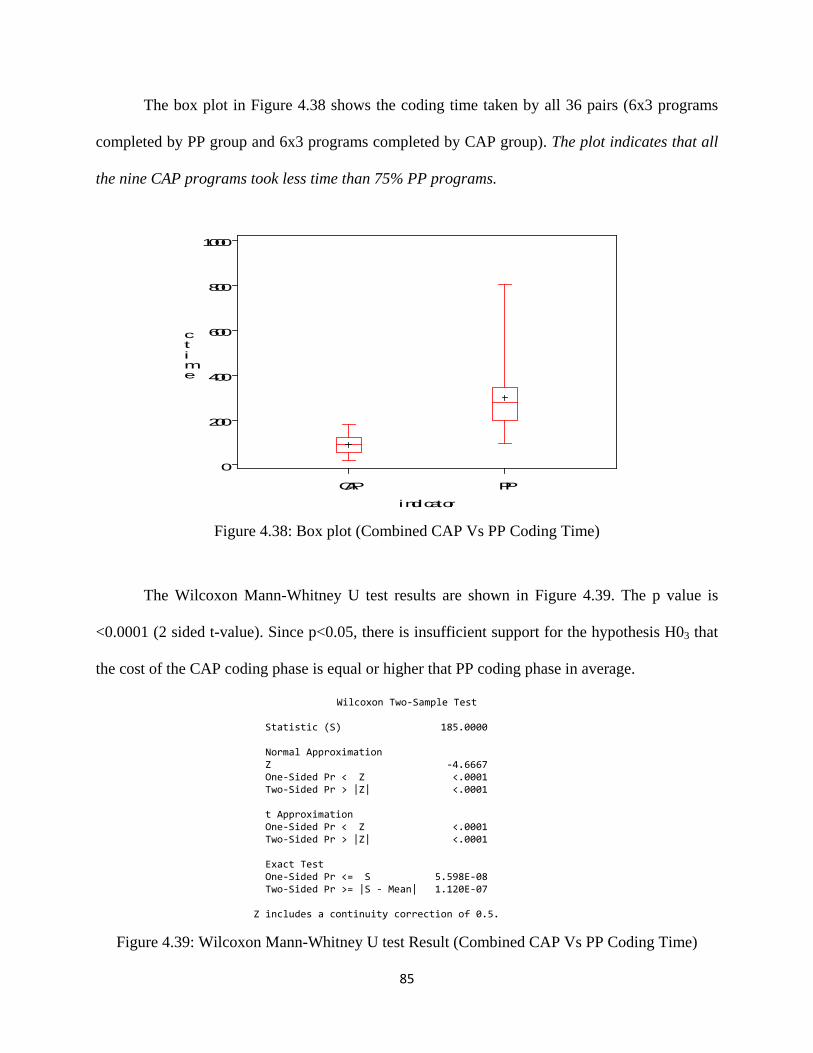
85



the nine CAP programs took less time than 75% PP programs.

Figure 4.38: Box plot (Combined CAP Vs PP Coding Time)

The Wilcoxon Mann-Whitney U test results are shown in Figure 4.39. The p value is

<0.0001 (2 sided t-value). Since p<0.05, there is insufficient support for the hypothesis H03 that

the cost of the CAP coding phase is equal or higher that PP coding phase in average.

Wilcoxon Two-Sample Test Statistic (S) 185.0000 Normal Approximation Z -4.6667 One-Sided Pr < Z <.0001 Two-Sided Pr > |Z| <.0001 t Approximation One-Sided Pr < Z <.0001 Two-Sided Pr > |Z| <.0001 Exact Test One-Sided Pr <= S 5.598E-08 Two-Sided Pr >= |S - Mean| 1.120E-07 Z includes a continuity correction of 0.5.

Figure 4.39: Wilcoxon Mann-Whitney U test Result (Combined CAP Vs PP Coding Time)

CAP PP

0

200

400

600

800

1000

ctime

indicator

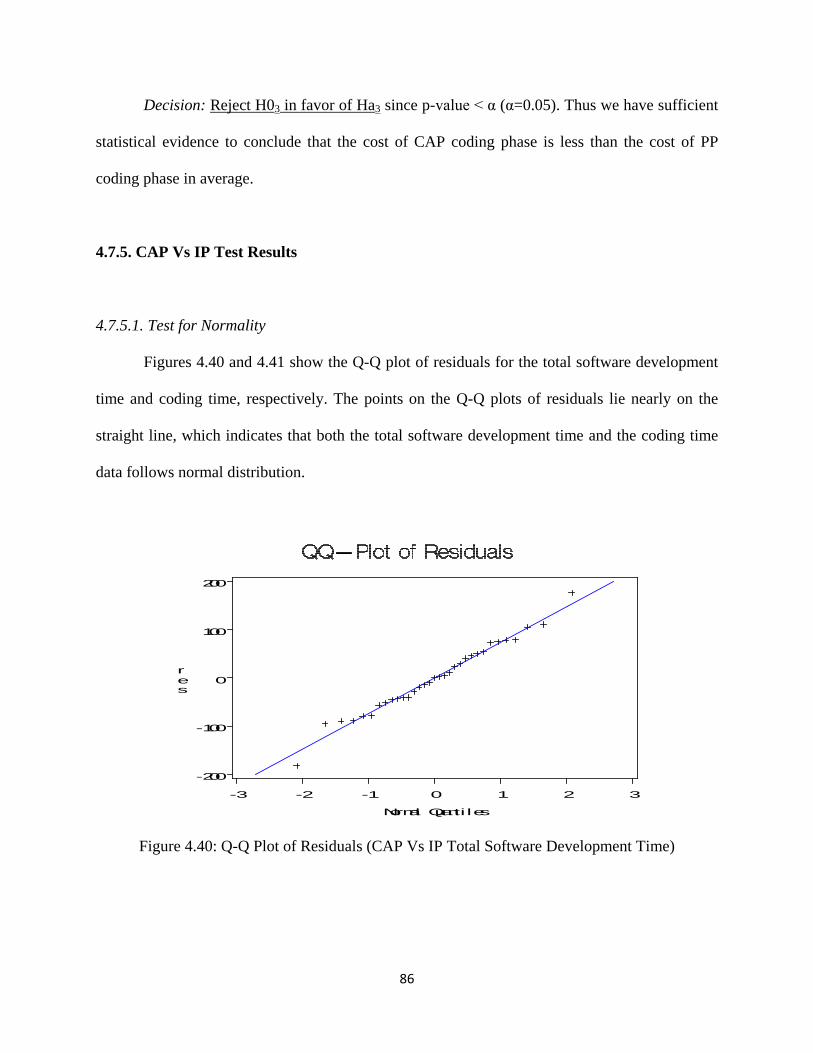
86




4.7.5. CAP Vs IP Test Results



time and coding time, respectively. The points on the Q-Q plots of residuals lie nearly on the

straight line, which indicates that both the total software development time and the coding time

data follows normal distribution.

Figure 4.40: Q-Q Plot of Residuals (CAP Vs IP Total Software Development Time)

-3 -2 -1 0 1 2 3

-200

-100

0

100

200

res

Normal Quanti les

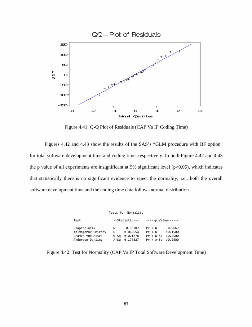
87

Figure 4.41: Q-Q Plot of Residuals (CAP Vs IP Coding Time)


for total software development time and coding time, respectively. In both Figure 4.42 and 4.43

the p value of all experiments are insignificant at 5% significant level (p>0.05), which indicates

that statistically there is no significant evidence to reject the normality; i.e., both the overall

software development time and the coding time data follows normal distribution.

Tests for Normality


Shapiro-Wilk W 0.98787 Pr < W 0.9667 Kolmogorov-Smirnov D 0.068654 Pr > D >0.1500 Cramer-von Mises W-Sq 0.021278 Pr > W-Sq >0.2500 Anderson-Darling A-Sq 0.176827 Pr > A-Sq >0.2500

Figure 4.42: Test for Normality (CAP Vs IP Total Software Development Time)

-3 -2 -1 0 1 2 3

-150

-100

-50

0

50

100

150

res

Normal Quanti les

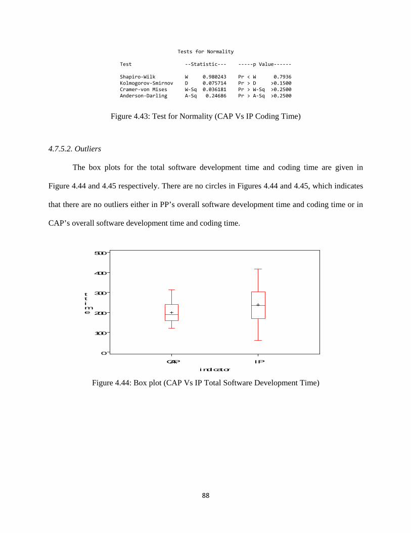
88

Tests for Normality


Shapiro-Wilk W 0.980243 Pr < W 0.7936 Kolmogorov-Smirnov D 0.075714 Pr > D >0.1500 Cramer-von Mises W-Sq 0.036181 Pr > W-Sq >0.2500 Anderson-Darling A-Sq 0.24686 Pr > A-Sq >0.2500

Figure 4.43: Test for Normality (CAP Vs IP Coding Time)

4.7.5.2. Outliers


Figure 4.44 and 4.45 respectively. There are no circles in Figures 4.44 and 4.45, which indicates



Figure 4.44: Box plot (CAP Vs IP Total Software Development Time)

CAP IP

0

100

200

300

400

500

ttime

indicator

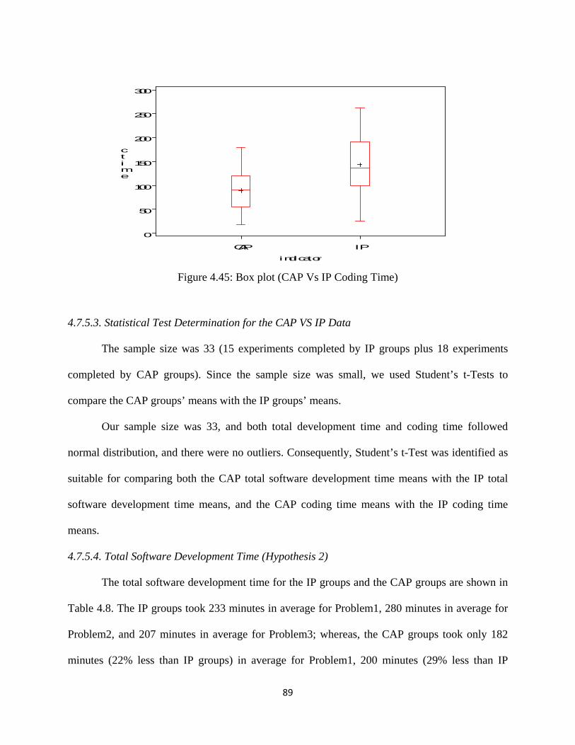
89

Figure 4.45: Box plot (CAP Vs IP Coding Time)

4.7.5.3. Statistical Test Determination for the CAP VS IP Data

The sample size was 33 (15 experiments completed by IP groups plus 18 experiments

completed by CAP groups). Since the sample size was small, we used Student’s t-Tests to

compare the CAP groups’ means with the IP groups’ means.

Our sample size was 33, and both total development time and coding time followed

normal distribution, and there were no outliers. Consequently, Student’s t-Test was identified as

suitable for comparing both the CAP total software development time means with the IP total

software development time means, and the CAP coding time means with the IP coding time

means.


The total software development time for the IP groups and the CAP groups are shown in

Table 4.8. The IP groups took 233 minutes in average for Problem1, 280 minutes in average for


minutes (22% less than IP groups) in average for Problem1, 200 minutes (29% less than IP

CAP IP

0

50

100

150

200

250

300

ctime

indicator

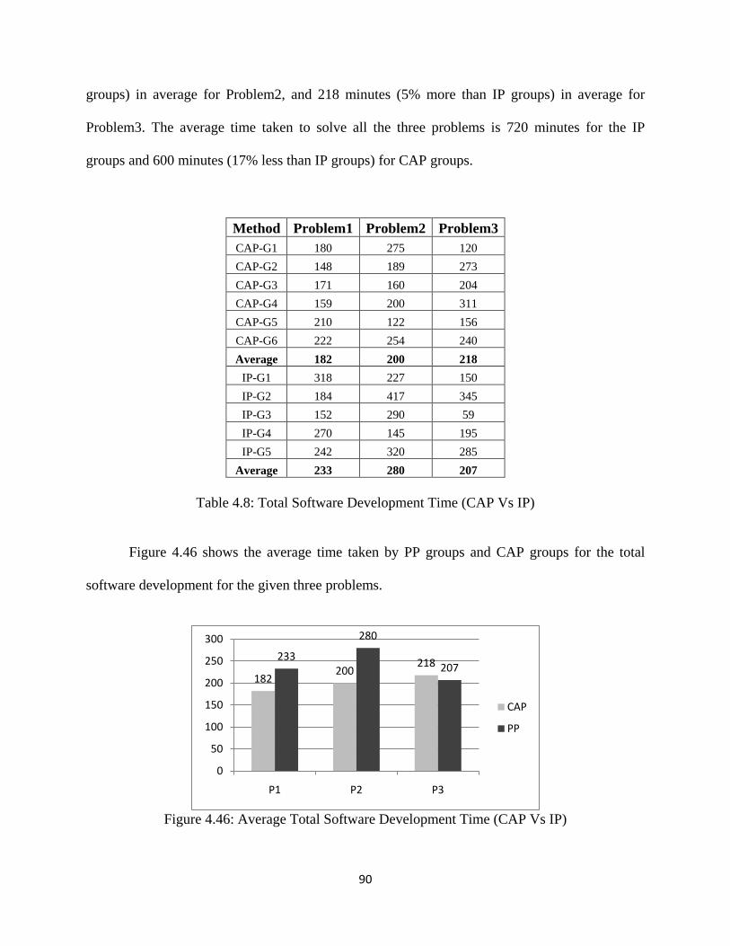
90

groups) in average for Problem2, and 218 minutes (5% more than IP groups) in average for

Problem3. The average time taken to solve all the three problems is 720 minutes for the IP

groups and 600 minutes (17% less than IP groups) for CAP groups.

Method Problem1 Problem2 Problem3 CAP-G1 180 275 120 CAP-G2 148 189 273 CAP-G3 171 160 204 CAP-G4 159 200 311 CAP-G5 210 122 156 CAP-G6 222 254 240 Average 182 200 218

IP-G1 318 227 150 IP-G2 184 417 345 IP-G3 152 290 59 IP-G4 270 145 195 IP-G5 242 320 285

Average 233 280 207

Table 4.8: Total Software Development Time (CAP Vs IP)



Figure 4.46: Average Total Software Development Time (CAP Vs IP)

182200

218233

280

207

0

50

100

150

200

250

300

P1 P2 P3

CAP

PP

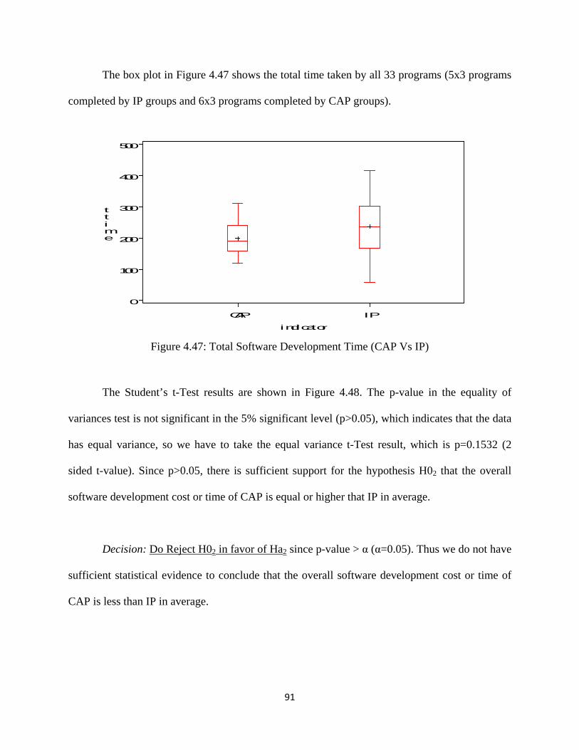
91

The box plot in Figure 4.47 shows the total time taken by all 33 programs (5x3 programs

completed by IP groups and 6x3 programs completed by CAP groups).

Figure 4.47: Total Software Development Time (CAP Vs IP)


variances test is not significant in the 5% significant level (p>0.05), which indicates that the data

has equal variance, so we have to take the equal variance t-Test result, which is p=0.1532 (2

sided t-value). Since p>0.05, there is sufficient support for the hypothesis H02 that the overall

software development cost or time of CAP is equal or higher that IP in average.

Decision: Do Reject H02 in favor of Ha2 since p-value > α (α=0.05). Thus we do not have

sufficient statistical evidence to conclude that the overall software development cost or time of

CAP is less than IP in average.

CAP IP

0

100

200

300

400

500

ttime

indicator

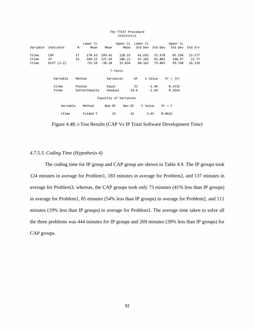
92

The TTEST Procedure Statistics

Lower CL Upper CL Lower CL Upper CL Variable indicator N Mean Mean Mean Std Dev Std Dev Std Dev Std Err ttime CAP 17 170.63 199.41 228.19 41.691 55.978 85.194 13.577 ttime IP 16 189.15 237.69 286.22 67.282 91.081 140.97 22.77 ttime Diff (1-2) -91.59 -38.28 15.034 60.162 75.043 99.768 26.139 T-Tests Variable Method Variances DF t Value Pr > |t| ttime Pooled Equal 31 -1.46 0.1532 ttime Satterthwaite Unequal 24.6 -1.44 0.1614 Equality of Variances Variable Method Num DF Den DF F Value Pr > F ttime Folded F 15 16 2.65 0.0622

Figure 4.48: t-Test Results (CAP Vs IP Total Software Development Time)


The coding time for IP group and CAP group are shown in Table 4.9. The IP groups took

124 minutes in average for Problem1, 183 minutes in average for Problem2, and 137 minutes in

average for Problem3; whereas, the CAP groups took only 73 minutes (41% less than IP groups)

in average for Problem1, 85 minutes (54% less than IP groups) in average for Problem2, and 111

minutes (19% less than IP groups) in average for Problem3. The average time taken to solve all

the three problems was 444 minutes for IP groups and 269 minutes (39% less than IP groups) for

CAP groups.

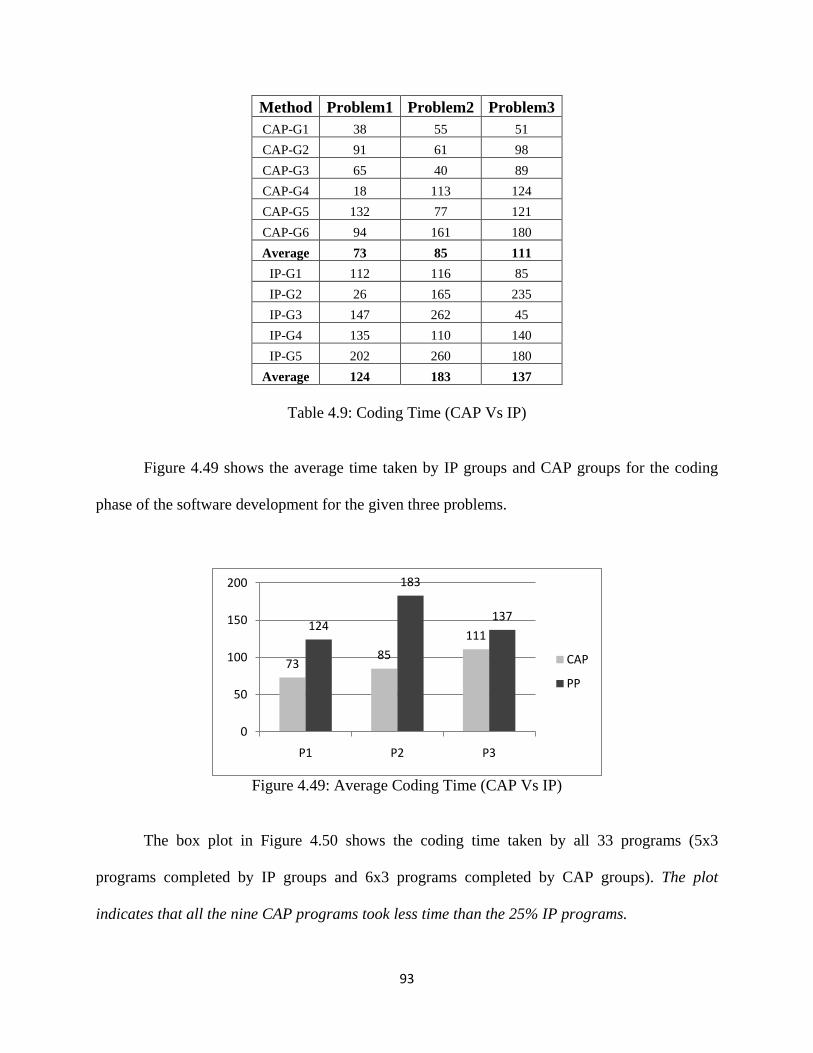
93

Method Problem1 Problem2 Problem3 CAP-G1 38 55 51 CAP-G2 91 61 98 CAP-G3 65 40 89 CAP-G4 18 113 124 CAP-G5 132 77 121 CAP-G6 94 161 180 Average 73 85 111

IP-G1 112 116 85 IP-G2 26 165 235 IP-G3 147 262 45 IP-G4 135 110 140 IP-G5 202 260 180

Average 124 183 137

Table 4.9: Coding Time (CAP Vs IP)

Figure 4.49 shows the average time taken by IP groups and CAP groups for the coding


Figure 4.49: Average Coding Time (CAP Vs IP)

The box plot in Figure 4.50 shows the coding time taken by all 33 programs (5x3

programs completed by IP groups and 6x3 programs completed by CAP groups). The plot

indicates that all the nine CAP programs took less time than the 25% IP programs.

7385

111124

183

137

0

50

100

150

200

P1 P2 P3

CAP

PP

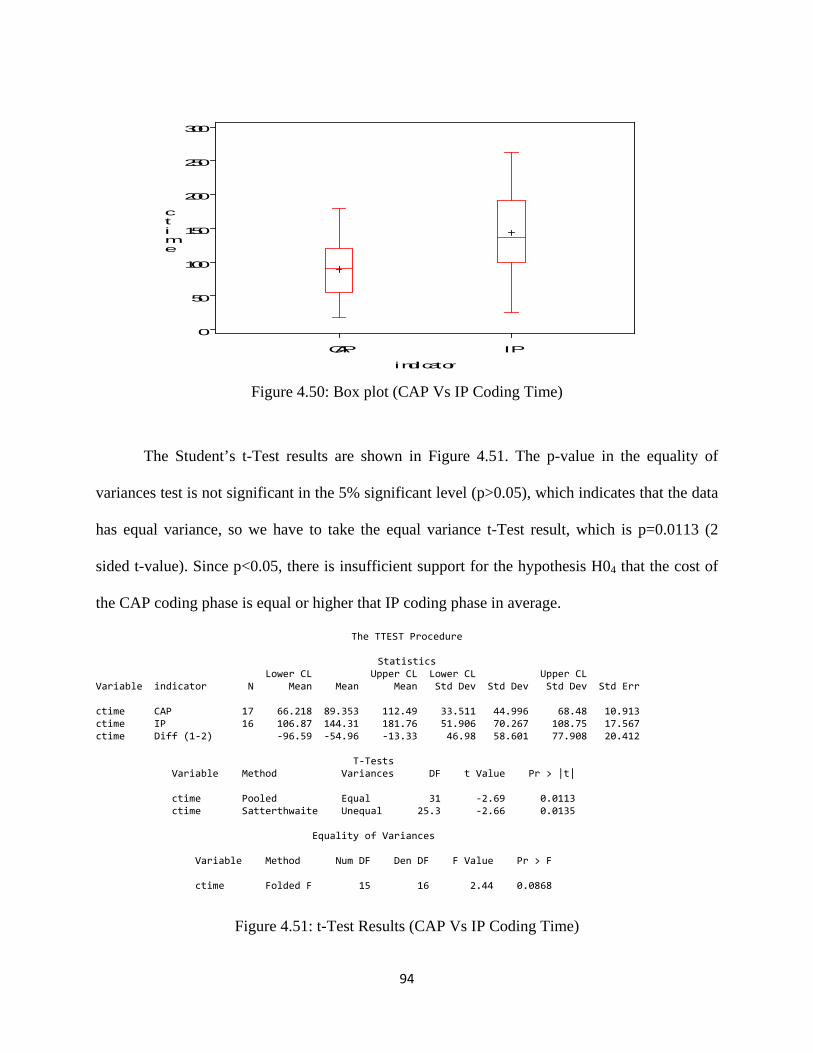
94

Figure 4.50: Box plot (CAP Vs IP Coding Time)


variances test is not significant in the 5% significant level (p>0.05), which indicates that the data

has equal variance, so we have to take the equal variance t-Test result, which is p=0.0113 (2

sided t-value). Since p<0.05, there is insufficient support for the hypothesis H04 that the cost of

the CAP coding phase is equal or higher that IP coding phase in average.

The TTEST Procedure

Statistics Lower CL Upper CL Lower CL Upper CL Variable indicator N Mean Mean Mean Std Dev Std Dev Std Dev Std Err ctime CAP 17 66.218 89.353 112.49 33.511 44.996 68.48 10.913 ctime IP 16 106.87 144.31 181.76 51.906 70.267 108.75 17.567 ctime Diff (1-2) -96.59 -54.96 -13.33 46.98 58.601 77.908 20.412 T-Tests Variable Method Variances DF t Value Pr > |t| ctime Pooled Equal 31 -2.69 0.0113 ctime Satterthwaite Unequal 25.3 -2.66 0.0135 Equality of Variances Variable Method Num DF Den DF F Value Pr > F ctime Folded F 15 16 2.44 0.0868

Figure 4.51: t-Test Results (CAP Vs IP Coding Time)

CAP IP

0

50

100

150

200

250

300

ctime

indicator

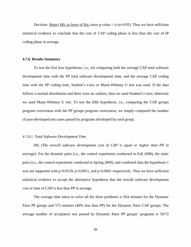
95


statistical evidence to conclude that the cost of CAP coding phase is less than the cost of IP


4.7.6. Results Summary

To test the first four hypotheses, i.e., for comparing both the average CAP total software

development time with the PP total software development time, and the average CAP coding

time with the PP coding time, Student’s t-test or Mann-Whitney U test was used. If the data

follows a normal distribution and there were no outliers, then we used Student’s t-test; otherwise

we used Mann-Whitney U test. To test the fifth hypothesis, i.e., comparing the CAP groups

program correctness with the PP groups program correctness, we simply compared the number

of post-developed test cases passed by programs developed by each group.

4.7.6.1. Total Software Development Time

H01 (The overall software development cost of CAP is equal or higher than PP in

average): For the dynamic pairs (i.e., the control experiment conducted in Fall 2008), the static

pairs (i.e., the control experiment conducted in Spring 2009), and combined data the hypothesis 1

was not supported with p=0.0129, p=0.0011, and p<0.0001 respectively. Thus we have sufficient

statistical evidence to accept the alternative hypothesis that the overall software development

cost or time of CAP is less than PP in average.

The average time taken to solve all the three problems is 954 minutes for the Dynamic

Pairs PP groups and 573 minutes (40% less than PP) for the Dynamic Pairs CAP groups. The

average number of acceptance test passed by Dynamic Pairs PP groups’ programs is 59/72

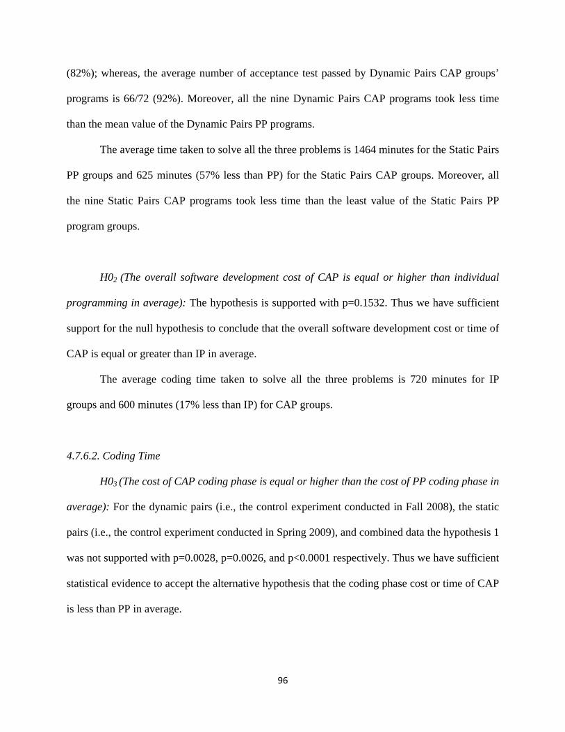
96

(82%); whereas, the average number of acceptance test passed by Dynamic Pairs CAP groups’

programs is 66/72 (92%). Moreover, all the nine Dynamic Pairs CAP programs took less time

than the mean value of the Dynamic Pairs PP programs.

The average time taken to solve all the three problems is 1464 minutes for the Static Pairs

PP groups and 625 minutes (57% less than PP) for the Static Pairs CAP groups. Moreover, all

the nine Static Pairs CAP programs took less time than the least value of the Static Pairs PP

program groups.

H02 (The overall software development cost of CAP is equal or higher than individual

programming in average): The hypothesis is supported with p=0.1532. Thus we have sufficient

support for the null hypothesis to conclude that the overall software development cost or time of

CAP is equal or greater than IP in average.

The average coding time taken to solve all the three problems is 720 minutes for IP

groups and 600 minutes (17% less than IP) for CAP groups.

4.7.6.2. Coding Time

H03 (The cost of CAP coding phase is equal or higher than the cost of PP coding phase in

average): For the dynamic pairs (i.e., the control experiment conducted in Fall 2008), the static

pairs (i.e., the control experiment conducted in Spring 2009), and combined data the hypothesis 1

was not supported with p=0.0028, p=0.0026, and p<0.0001 respectively. Thus we have sufficient

statistical evidence to accept the alternative hypothesis that the coding phase cost or time of CAP

is less than PP in average.

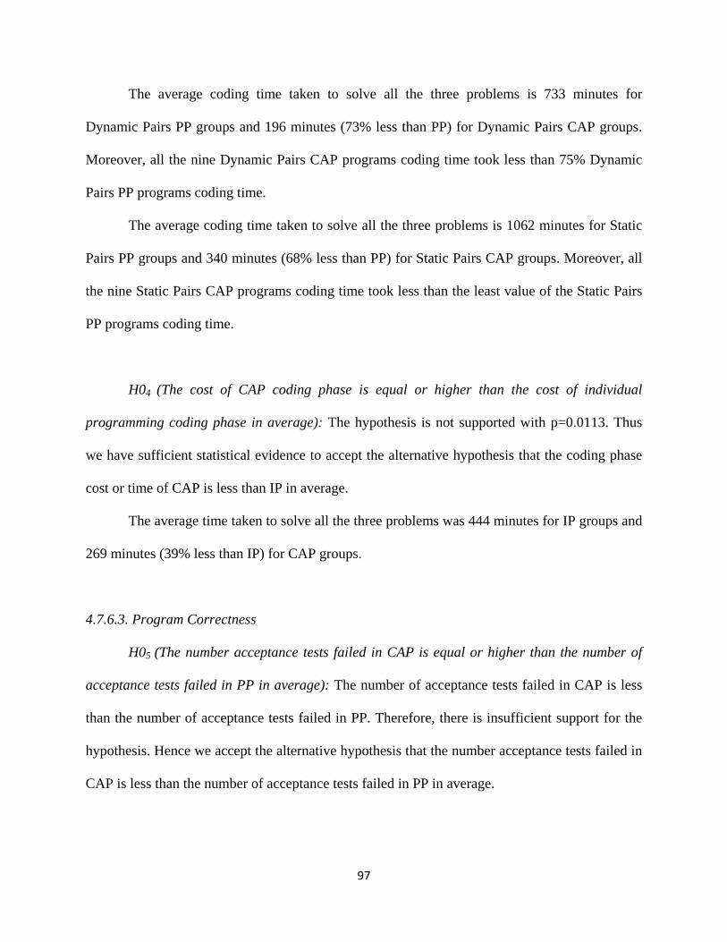
97

The average coding time taken to solve all the three problems is 733 minutes for

Dynamic Pairs PP groups and 196 minutes (73% less than PP) for Dynamic Pairs CAP groups.

Moreover, all the nine Dynamic Pairs CAP programs coding time took less than 75% Dynamic

Pairs PP programs coding time.

The average coding time taken to solve all the three problems is 1062 minutes for Static

Pairs PP groups and 340 minutes (68% less than PP) for Static Pairs CAP groups. Moreover, all

the nine Static Pairs CAP programs coding time took less than the least value of the Static Pairs

PP programs coding time.

H04 (The cost of CAP coding phase is equal or higher than the cost of individual

programming coding phase in average): The hypothesis is not supported with p=0.0113. Thus

we have sufficient statistical evidence to accept the alternative hypothesis that the coding phase

cost or time of CAP is less than IP in average.

The average time taken to solve all the three problems was 444 minutes for IP groups and

269 minutes (39% less than IP) for CAP groups.

4.7.6.3. Program Correctness

H05 (The number acceptance tests failed in CAP is equal or higher than the number of

acceptance tests failed in PP in average): The number of acceptance tests failed in CAP is less

than the number of acceptance tests failed in PP. Therefore, there is insufficient support for the

hypothesis. Hence we accept the alternative hypothesis that the number acceptance tests failed in

CAP is less than the number of acceptance tests failed in PP in average.

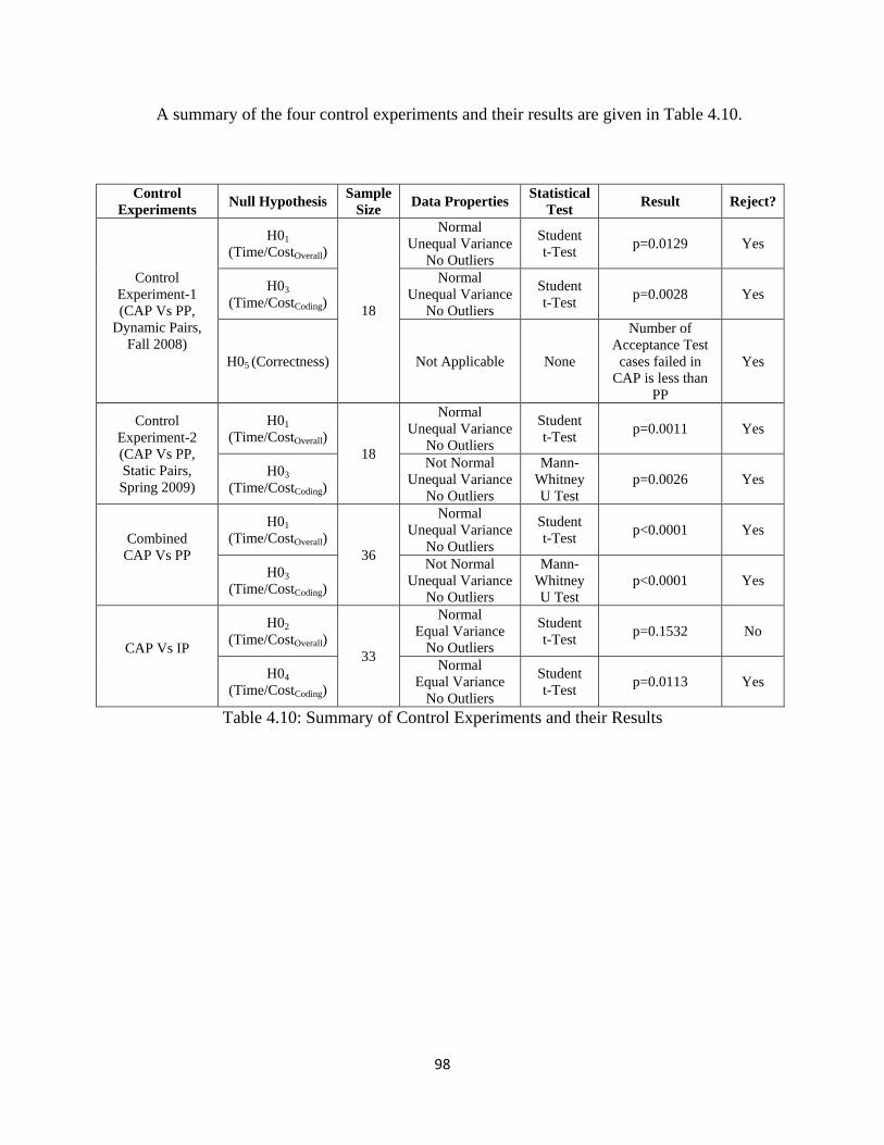
98

A summary of the four control experiments and their results are given in Table 4.10.

Control Experiments Null Hypothesis Sample

Size Data Properties Statistical Test Result Reject?

Control Experiment-1 (CAP Vs PP,

Dynamic Pairs, Fall 2008)

H01 (Time/CostOverall)

18

Normal Unequal Variance

No Outliers

Student t-Test p=0.0129 Yes

H03 (Time/CostCoding)


No Outliers


H05 (Correctness) Not Applicable None

Number of Acceptance Test cases failed in

CAP is less than PP

Yes

Control Experiment-2 (CAP Vs PP, Static Pairs, Spring 2009)


18


No Outliers



Not Normal Unequal Variance

No Outliers

Mann-Whitney U Test

p=0.0026 Yes

Combined CAP Vs PP


36


No Outliers

Student t-Test p<0.0001 Yes


Not Normal Unequal Variance

No Outliers

Mann-Whitney U Test

p<0.0001 Yes

CAP Vs IP


33

Normal Equal Variance

No Outliers

Student t-Test p=0.1532 No


Normal Equal Variance

No Outliers


Table 4.10: Summary of Control Experiments and their Results

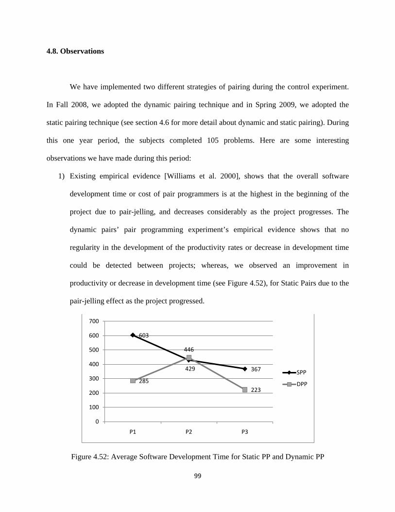
99

4.8. Observations

We have implemented two different strategies of pairing during the control experiment.

In Fall 2008, we adopted the dynamic pairing technique and in Spring 2009, we adopted the

static pairing technique (see section 4.6 for more detail about dynamic and static pairing). During

this one year period, the subjects completed 105 problems. Here are some interesting

observations we have made during this period:

1) Existing empirical evidence [Williams et al. 2000], shows that the overall software

development time or cost of pair programmers is at the highest in the beginning of the

project due to pair-jelling, and decreases considerably as the project progresses. The

dynamic pairs’ pair programming experiment’s empirical evidence shows that no

regularity in the development of the productivity rates or decrease in development time

could be detected between projects; whereas, we observed an improvement in

productivity or decrease in development time (see Figure 4.52), for Static Pairs due to the

pair-jelling effect as the project progressed.

Figure 4.52: Average Software Development Time for Static PP and Dynamic PP

603

429 367

285

446

223

0

100

200

300

400

500

600

700

P1 P2 P3

SPP

DPP

100

2) The static PP helps the programmers to solve routine or similar kinds of problems

(Problem1 and Problem2 in our case) faster than dynamic PP programmers as shown in

Figure 4.52. But, the dynamic pairing (both the dynamic PP and the dynamic CAP) helps

the programmers to solve a new kind of problem (problem 3 in our case) faster than its

static counterpart. This we can observe from Figure 4.52 and Figure 4.53.

Figure 4.53: Average Software Development Time for Static CAP and Dynamic CAP

3) The productivity of the dynamic PP groups is better than static PP groups. The average

time taken to solve all three problems for dynamic PP groups is 954 minutes; whereas, it

took 1399 minutes (32% more than dynamic PP groups) for static PP groups. At the same

time, we did not observe any difference in productivity between static CAP groups and

dynamic CAP groups; the average time taken to solve all three problems for dynamic

CAP groups and static CAP groups is 573 minutes and 578 minutes respectively.

140

178

260

166

208

199

0

50

100

150

200

250

300

P1 P2 P3

SCAP

DCAP

101

4) One of the major benefits of collaborative programming is pair-pressure [Williams et al.

2000]. During the entire control experiment period we observed the existence of pair-

pressure among both the CAP programmers and the pair programmers. When they met

both partners worked intensively and were motivated to complete their assigned task

within the specified time period. This motivation was lagging with individual

programmers; some individual programmers even withdrew in the middle of the

experiment. At the same time, we did not observed any gain in productivity and/or

quality improvements by the pair programmers due to pair-pressure as indicated by

[Williams et al. 2000].

5) We have observed that the pairs in CAP discuss more in design time and create concrete

designs in contrast to their PP counterparts. The pairs in CAP also know that after the

design phase they will play on adversarial role in the implementation stage (the goal of

the implementer is to build working software, whereas the goal of the tester is to break

the software in CAP). We believe this forces them to discuss more in the design stage

before moving to the implementation stage. Since the PP developers know that they are

going to have a partner throughout the entire development phases, we feel that the

confidence of having a partner in the development stage turns into overconfidence and

they do not discuss much in the design stage. Furthermore, this overconfidence leads to a

design that is not concrete which in turn, causes them to change their design more often

in the coding phase and spend 50% more time than their CAP counter parts.

102

5. CONCLUSIONS AND FUTURE WORK

5.1. Conclusions

In this research we have proposed a new stable and reliable agile software development

methodology called Collaborative-Adversarial Pair (CAP) programming. We see CAP as an

alternative to traditional pair programming in situations where pair programming is not

beneficial or is not possible to practice. The CAP was evaluated against traditional pair

programming and individual programming in terms of productivity and program correctness. The

empirical evidence shows that traditional pair programming is an expensive technology and does

not necessarily produce programs with better quality as claimed by the pair programming

advocates.

The empirical evidence shows that better quality programs can be produced in 40% less

time using the dynamic pairs CAP programming technique than the dynamic pair programming

technique, better or equal quality programs can be produced in 57% less time using the static

pairs CAP programming technique than the static pair programming technique, and overall,

better or equal quality programs can be produced with a much cheaper cost (50% less overall

software development time than traditional PP) using the CAP programming technique. The

empirical evidence also shows that CAP is a cheaper technology than individual programming;

using CAP we can produce programs of equal or better quality with 17% reduction in overall

software development cost on average.

103

The empirical evidence shows that better or equal quality code can be produced in 73%

less time using the dynamic pairs CAP programming technique than the dynamic pair

programming technique, better or equal quality code can be produced in 68% less time using the

static pairs CAP programming technique than the static pair programming technique, and overall,

better or equal quality code can be produced with a much cheaper cost (70% less than traditional

PP) using CAP programming technique. The empirical evidence also shows that CAP is a

cheaper technology than individual programming; using CAP we can produce code of equal or

better quality with 39% reduction in coding cost on average.

It is expected that CAP will retain the advantages of pair programming while at the same

time downplaying the disadvantages. In CAP, units are implemented by single developers

(whereas two developers are developing a unit in pair programming) and functional test cases

can be developed in parallel with unit implementation. This, in turn, reduces the overall project

development interval. The CAP testing procedure judiciously combines the functional (black

box) and structural (white box) testing, which provides the software with the confidence of

functional testing and the measurement of structural testing. The CAP allows us to confidently

test and add the purchased or contracted software modules to the existing software. Finally, the

functional test cases in the CAP allow us to change the implementation without changing the test

cases and vice-versa.

104

5.2. Future Work

• The external validity, the ability of the experimental results to apply to the world outside

the research environment – over variations in persons, settings, treatments, and outcomes,

of the empirical research design is very important for any research study. We have

carefully planned our CAP validation to meet these external validity requirements.

Though the software development environment provided by us closely matches the

industrial software development environment, clearly the experimental system and tasks

in this experiment were small compared with industrial software systems and tasks.

Therefore, we cannot rule out the possibility that the observed results would have been

different if the system and tasks had been larger. Hence, validation of the results with

professional programmers in an industrial setting would be beneficial.

• We aim to design, build, and test a stable and reliable new agile software development

methodology called Team Collaborative-Adversarial Pair (TCAP) Programming, which

is suitable for the software development teams. To achieve our goal, we employ the CAP

process as a basic building block to design and build the TCAP.

• Currently we have integrated and validated the CAP methodology into the Extreme

Programming process. In the future, we are planning to integrate the CAP into the other

agile development methodologies as well.

• We are also planning to develop tool set to support CAP methodology.

105

REFERENCES [Abrahamsson et

al. 2004]

Pekka Abrahamsson, Antti Hanhineva, Hanna Hulkko, Tuomas Ihme,

Juho Jäälinoja, Mikko Korkala, Juha Koskela, Pekka Kyllönen, and

Outi Salo. Mobile-D: An Agile Approach for Mobile Application

Development, OOPSLA’04, Oct. 24–28, 2004, Vancouver, British

Columbia, Canada.

ACM 1-58113-833-4/04/0010.

[Al-Kilidar et al.

2005]

Al-Kilidar, H., Parkin, P., Aurum, A., Jeffery, R. Evaluation of effects

of pair work on quality of designs. In: Proceedings of the 2005

Australian Software Engineering Conference (ASWEC 2005)

Brisbane Australia. IEEE CS Press, pp. 78–87.

[Anderson et al.

1998]

A. Anderson, R. Beattie, et al., Chrysler Goes to “Extreme”,

http://www.xprogramming.com/publications/dc9810cs.pdf

[Arisholm et al.

2007]

Erik Arisholm, Hans Gallis, Tore Dyba, and Dag I.K. Sjøberg,

Evaluating Pair Programming with Respect to System Complexity and

Programmer Expertise, IEEE Transactions on Software Engineering,

Vol. 33, No. 2, Feb 2007

[Astels 2003] David Astels, Test-Driven Development: A Practical Guide, Prentice

Hall, 2003.

[Bagley et al. Carole A. Bagley and C. Candace Chou, Collaboration and the

106

2007] Importance for Novices in Learning Java Computer Programming,

ITiCSE’07, June 23-27, 2007, Dundee, Scotland, United Kingdom.

[Beck et al. 1989] Kent Beck and Ward Cunningham, A Laboratory For Teaching

Object-Oriented Thinking, OOPSLA'89 Conference Proceedings

October 1-6, 1989, New Orleans, Louisiana.

[Beck 2000] Kent Beck, Extreme Programming Explained: An Embrace Change,

Addison-Wesley, 2000, ISBN 0201616416.

[Beck 2003] Kent Beck, Test-Driven Development: By Example, Addison-Wesley,

2003.S

[Boutin 2000] Karl Boutin. Introducing Extreme Programming in a Research and

Development Laboratory. Extreme Programming Examined, Addison-

Wesley, Chapter 25, pages 433-448.

[Canfora et al.

2006]

Canfora, G., Cimitile, A., Visaggio, C.A., Garcia, F., Piattini, M.,

Performances of pair designing on software evolution: a controlled

experiment. In: Proceedings of the 10th European Conference on

Software Maintenance and Reengineering, CSMR 2006, 22–24

March, Bari, Italy, pp. 197-205.

[Canfora et al.

2007]

Gerardo Canfora, Aniello Cimitile, Felix Garcia, Mario Piattini, and

Corrado Aaron Visaggio, Evaluating performances of pair designing

in industry, The Journal of Systems and Software 80 (2007) 1317–

1327

[Cockburn et al.

2000]

Cockburn, Alistair & Williams, Laurie (2000), “The Costs and

Benefits of Pair Programming”, Proceedings of the First International

107

Conference on Extreme Programming and Flexible Processes in

Software Engineering (XP2000).

[Confer 2009] Personal e-mail communication

[Flor 1991] Flor, N., & Hutchins, E. Analyzing distributed cognition in software

teams: A case study of team programming during perfective software

maintenance. Proceedings of the fourth annual workshop on empirical

studies of programmers (pp. 36-59), 1991, Norwood, NJ: Ablex

Publishing.

[Hulkko et al.

2005]

Hanna Hulkko and Pekka Abrahamsson, A Multiple Case Study on

the Impact of Pair Programming on Product Quality, ICSE’05, May

15-21, 2005, St. Louis, Missouri, USA.

[Jensen 2003] http://www.stsc.hill.af.mil/crosstalk/2003/03/jensen.html

[Lippert et al.

2001]

Martin Lippert, Stefan Rooks, Henning Wolf, and Heinz Zullighoven.

JWAM and XP: Using XP for Framework Development. Extreme

Programming Examined, Addison-Wesley, Chapter 7, pages 103-117.

[Lui et al. 2003] Lui, K., Chan, K., 2003. When does a pair outperform two

individuals? In: Proceedings of XP 2003LNCS. Springer-Verlag, pp.

225-233.

[Lui et al. 2006] Kim Man Lui and Keith C.C. Chan, Pair programming productivity:

Novice-novice vs. expert-expert, Int. J. Human-Computer Studies 64

(2006) 915-925.

[Martin 2003]

Robert C. Martin, Agile Software Development: Principles, Patterns,

and Practices, Prentice Hall, 2003.

http://www.stsc.hill.af.mil/crosstalk/2003/03/jensen.html�

108

[McDowell et al.

2002]

McDowell, C., Werner, L., Bullock, H., Fernald, J., 2002. The effects

of pair-programming on performance in an introductory programming

course. In: Proceedings of the 33rd SIGCSE Technical Symposium on

Computer Science Education. ACM, Cincinnati, KY, USA, pp. 38–42.

[Mendes et al.

2005]

Emilia Mendes, Lubna Basil Al-Fakhri, and Andrew Luxton-Reilly,

Investigating Pair-Programming in a 2nd-year Software Development

and Design Computer Science Course, ITiCSE’05, June 27–29, 2005,

Monte de Caparica, Portugal.

[Muller 2004] MATTHIAS M. MULLER, Are Reviews an Alternative to Pair

Programming? Empirical Software Engineering, 9, 335–351, 2004.

[Muller 2005] Matthias M. Muller, Two controlled experiments concerning the

comparison of pair programming to peer review, The Journal of

Systems and Software 78 (2005) 166–179

[Nawrocki et al.

2001]

Nawrocki, J. and Wojciechowski, A., 2001. Experimental Evaluation

of pair programming. In: Proceedings of the European Software

Control and Metrics Conference (ESCOM 2001). ESCOM Press,

2001, pp. 269– 276.

[Nosek 1998] John T. Nosek, The Case for Collaborative Programming,

Communications of the ACM March 1998/Vol. 41, No. 3

[perl 2004] http://use.perl.org/~inkdroid/journal/17066

[Pressman 2005] Roger S. Pressman. Software Engineering: A Practitioner’s Approach,

sixth edition, McGraw Hill, 2005.

[Umphress 2008] Umphress, David. Personal Communication.

http://use.perl.org/~inkdroid/journal/17066�

109

[Vanhanen et al.

2005]

Jari Vanhanen and Casper Lassenius, Effects of Pair Programming at

the Development Team Level: An Experiment, 2005 IEEE

[Wake 2002] William C. Wake, Extreme Programming Explored, Addison –

Wesley, 2002.

[Wells et al. 2001] Don Wells and Trish Buckley. The VCAPS Project: An Example of

Transitioning to XP. Extreme Programming Examined, Addison-

Wesley, Chapter 23, pages 399-421.

[Wiki] http://c2.com/cgi/wiki?PairProgrammingFacilities

[Williams 2001] Laurie Williams, Integrating pair programming into a software

development process, Software Engineering Education and Training,

2001. Proceedings. 14th Conference on Volume, Issue, 2001

Page(s):27 – 36

[Williams et al.

2000]

Laurie Williams, Robert R. Kessler, Ward Cunningham, Ron Jeffries,

Strengthening the Case for Pair Programming, July/August 2000 IEEE

SOFTWARE

[Williams et al.

2000b]

Laurie A. Williams and Robert R. Kessler, All I really need to know

about pair programming I learned in kindergarten, Communications of

the ACM, Volume 43 , Issue 5 (May 2000), Pages: 108 - 114

[Williams et al.

2003]

Laurie Williams and Robert Kessler, Pair Programming Illuminated.

Addison-Wesley, 2003, ISBN 0-201-74576-3.

[Wilson et al.

1993]

Wilson, J., Hoskin, N., Nosek, J., 1993. The benefits of collaboration

for student programmers. In: Proceedings 24th SIGCSE Technical

Symposium on Computer Science Education, pp. 160–164.

http://c2.com/cgi/wiki?PairProgrammingFacilities�

http://en.wikipedia.org/wiki/Special:BookSources/0201745763�

110

[XP 1999] http://www.extremeprogramming.org/rules/pair.html

[Xu et al. 2006] Shaochun Xu, Vaclav Rajlich, Empirical Validation of Test-Driven

Pair Programming in Game Development, Proceedings of the 5th

IEEE/ACIS International Conference on Computer and Information

Science and 1st IEEE/ACIS International Workshop on Component-

Based Software Engineering, Software Architecture and Reuse (ICIS-

COMSAR’06)

http://www.extremeprogramming.org/rules/pair.html�

111

Appendix-A

Pair Programming Experiments Analyzed

112

S. No

Study Year Selected? Comments

1 Wilson et al. [Wilson et al., 1993] 1993 Y 2 Nosek [Nosek, 1998] 1998 Y 3 Williams et al. [Williams et al., 2000] 1999 Y 4 Nawrocki and Wojciechowski

[Nawrocki et al., 2001] 1999/ 2000

Y

5 McDowell et al [McDowell et al., 2002]

2000/ 2001

Y

6 Baheti et al. 2002 N Distributed PP experiment 7 Rostaher et al. 2002 Y 8 Heiberg et al. 2003 N Not PP Vs Solo experiment, it is a PP VS 2

person team experiment 9 Canfora et al. 2007 N Design phase only

10 Müller [Muller, 2005] 2002/ 2003

Y

11 Vanhanen and Lassenius [Vanhanen et al., 2005]

2004 Y

12 Madeyski 2006 N Design phase only 13 Müller [Muller 2006] 2005 Y 14 Monvorath et al. 2004,

2005 N Compares the PP Vs Inspection techniques

practiced only in Thailand. 15 Xu and Rajlich [Xu et al., 2006] 2005,

2006 Y

16 Canfora et al. 2005 N Each subjects performed both PP and solo programming alternatively

17 Arisholm et al. [Arisholm et al., 2007]

2001, 2004/ 2005

Y

18 Hulkko and Abrahamson [Hulkko et al, 2005]

2004 Y

19 Lui and Chan [Lui et al. 2006] 2005 N Repeat experiment compares Novice-Novice pairs against Expert-Expert pairs.

20 Jensen 1996 N Not PP Vs Solo experiment, only pairs experiment

21 Mendes et al. 2005 N PP used as a teaching tool 22 Carver et al. 2007 N PP used as a teaching tool 23 Carole and Chou 2007 N PP used as a teaching tool 24 Cliburn 2003 N PP used as a teaching tool 25 Phongpaibul and Boehm 2006 N Comparison of pair development and

software inspection in Thailand 26 McDowell et al. 2003 N PP used as a teaching tool 27 McDowell et al. 2003 N PP used as a teaching tool 28 Cubranic and Storey 2005 N Pairs of first year CS students used to

evaluate a prototype 29 Hanks et al. 2004 N PP used as a teaching tool 30 Gehringer 2003 N PP used as a teaching tool 31 Nagappan et al. 2003 N PP used as a teaching tool 32 Succi et al. 2001 N Only job satisfaction analysis 33 Bellini et al., 2005 N Design phase only 34 Al-Kilidar et al. 2005 N Design phase only 35 Canfora et al. 2006 N Design phase only

113

APPENDIX-B

IRB Documents

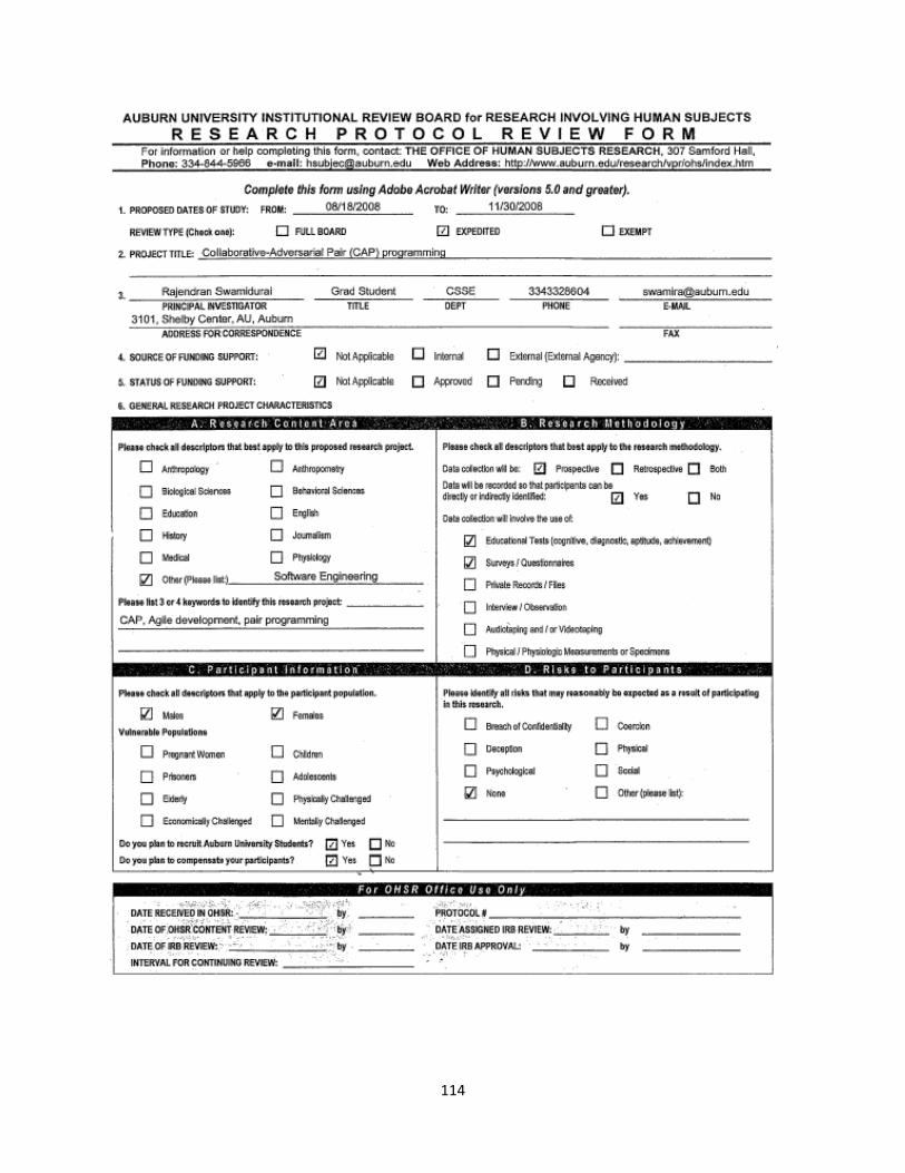
114

115

116

117

118

119

120

121

122

123

124

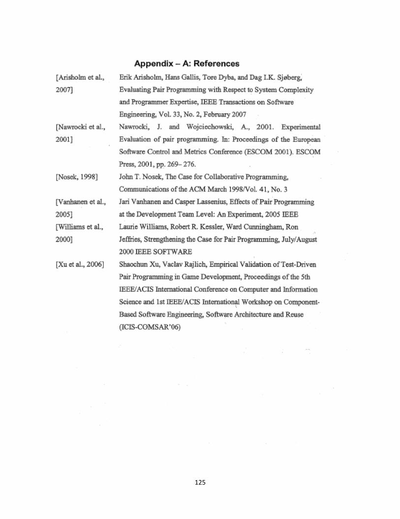
125

126

127

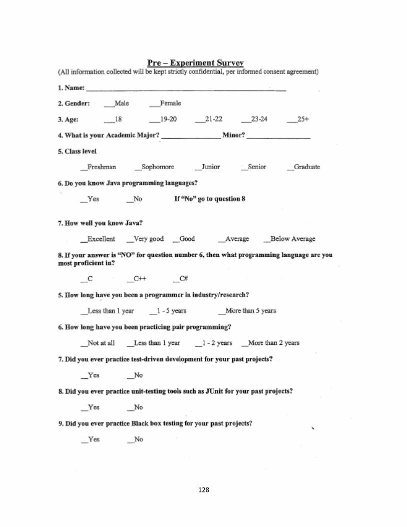
128

129

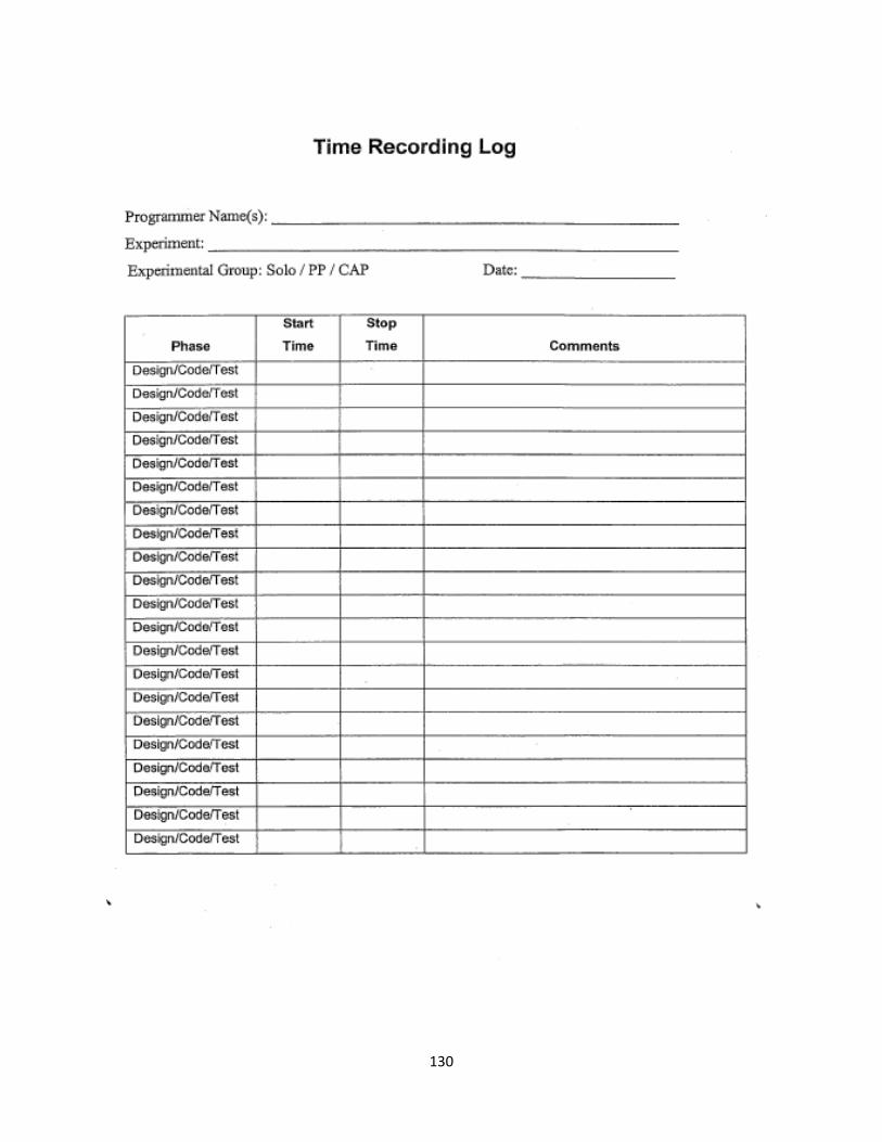
130

131

132

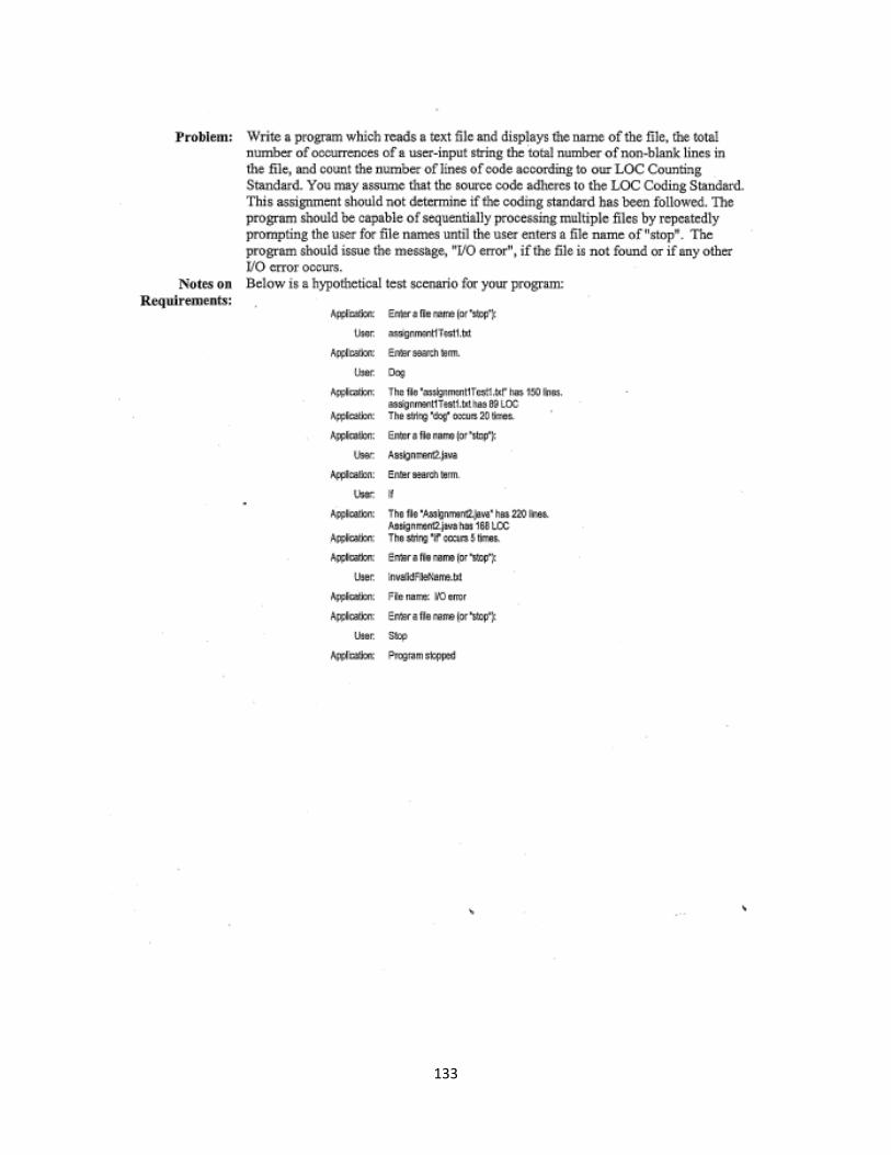
133

134

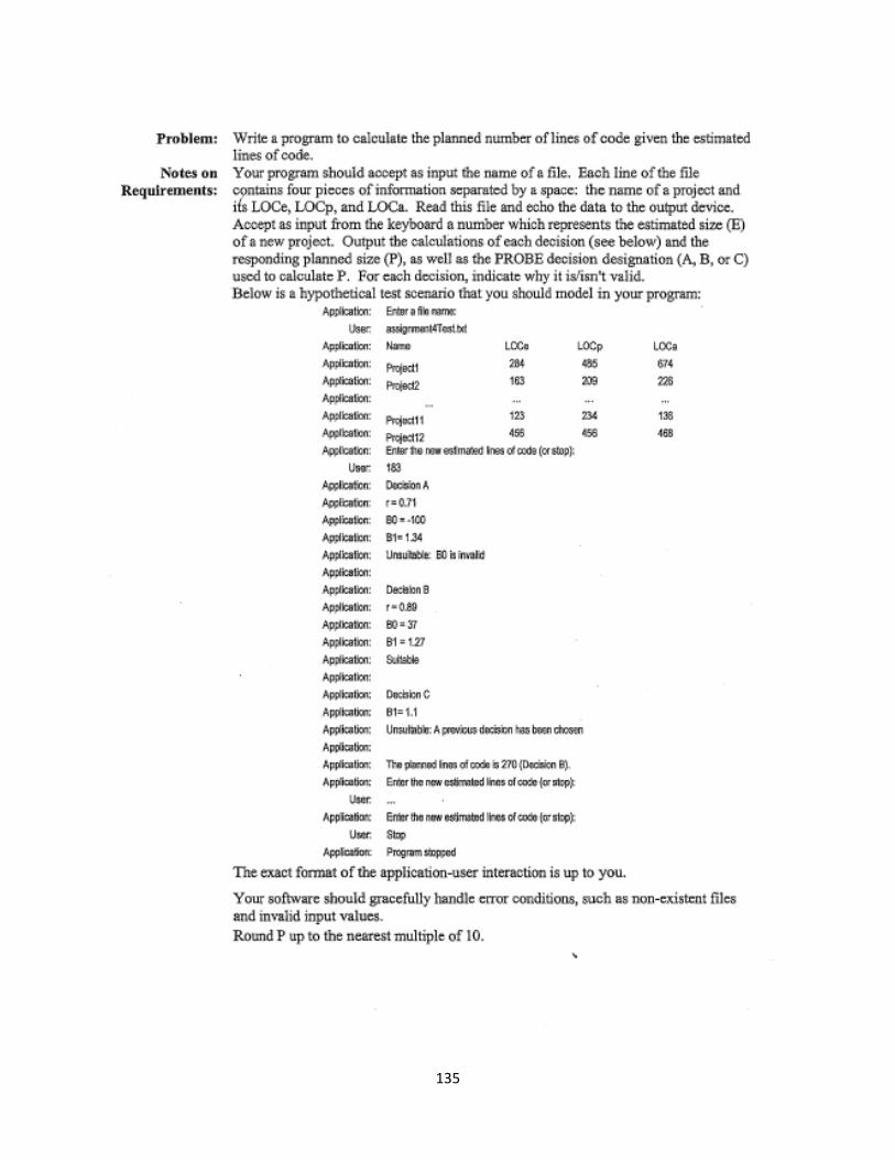
135

136

137

138

139

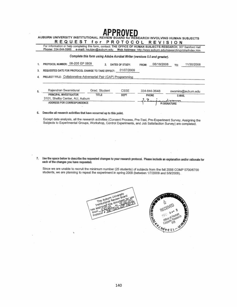
140

141

142

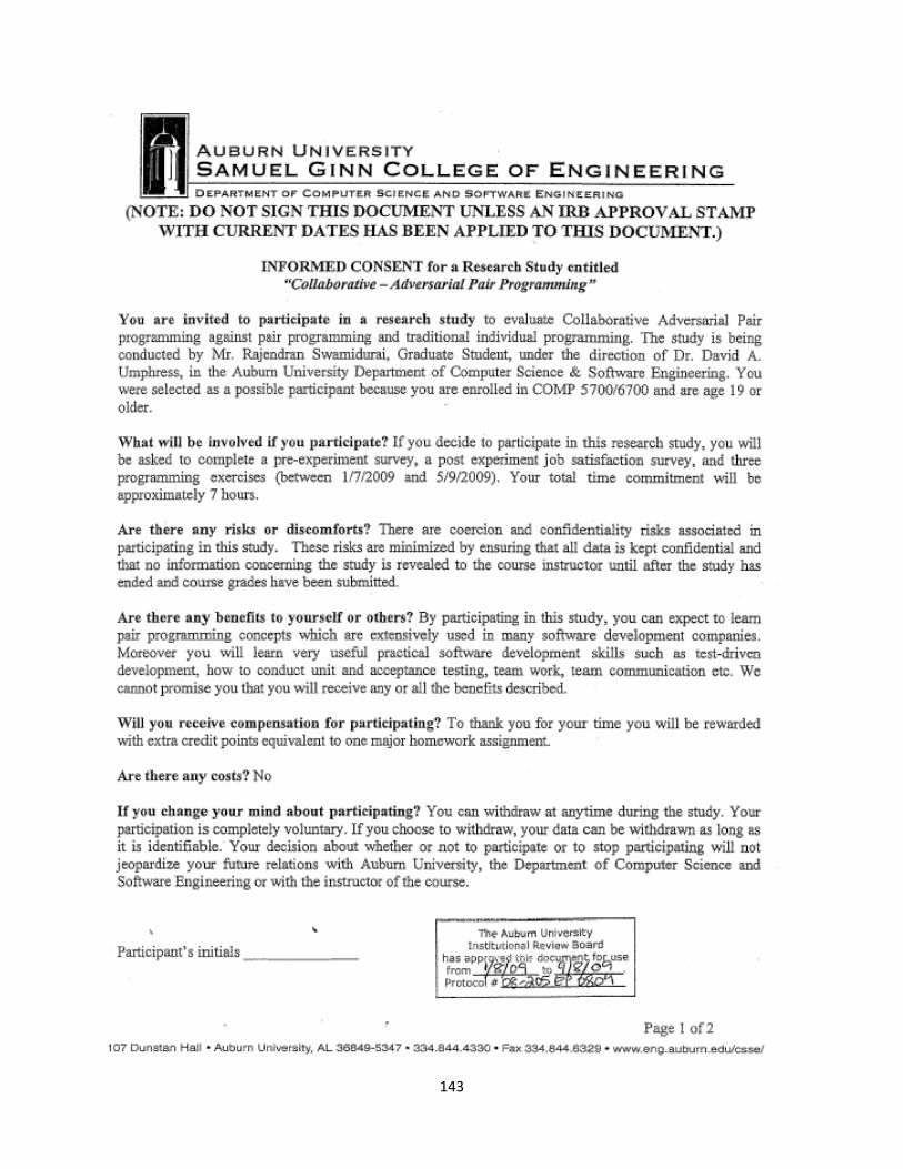
143

144