Coint - 1

Cointegration - general discussion

Definitions: A time series that requires d differences to get it stationary is said to be"integrated of order d". If the d difference has p AutoRegressive and q Movingth

Average terms, the differenced series is said to be ARMA(p,q) and the original Integratedseries to be ARIMA(p,d,q). Two series X and Y that are integrated of order d may, through lineart tcombination, produce a series which is stationary (or integrated of order+\ ,]> >

smaller than d) in which case we say that and are cointegrated and we refer to\ ]> >

Ð+ß ,Ñ as the cointegrating vector. Granger and Weis discuss this concept andterminology.

An example:

For example, if and are wages in two similar industries, we may find that\ ]> >

both are unit root processes. We may, however, reason that by virtue of the similar skillsand easy transfer between the two industries, the difference - cannot vary too far\ ]> >

from 0 and thus, certainly should not be a unit root process. The cointegrating vector isspecified by our theory to be or , or all of which areÐ"ß "Ñ Ð "ß "Ñ Ð-ß -Ñequivalent.

The test for cointegration here consists of simply testing the original series forunit roots, not rejecting the unit root null , then testing the - series and rejecting the\ ]> >

unit root null. We just use the standard D-F tables for all these tests. The reason we canuse these D-F tables is that the cointegrating vector was specified by our theory, notestimated from the data.

Numerical examples: ] œ E] I> >" >

1. Bivariate, stationary:

0 0Œ ” •Œ Œ ] "Þ# Þ$ /] Þ% Þ& ] /

œ ß]"> ">

#> #ß>" #>

"ß>"I µ> R ß

! % "! " $ Œ Œ

E M œ œ "Þ( Þ' Þ"# œ Ð Þ*ÑÐ Þ)Ñ"Þ# Þ$

Þ% Þ& - - - - -

--º º

#

this is note distribution has no impact )=>+>398+<C Ð I>

Coint - 2

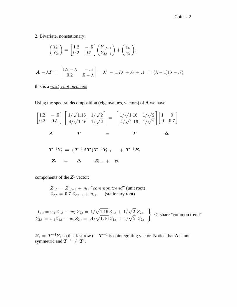
2. Bivariate, nonstationary:

0 2 0Œ ” •Œ Œ ] "Þ# Þ& /] Þ Þ& ] /

œ ß]"> ">

#> #ß>" #>

"ß>"

E M œ œ "Þ( Þ' Þ" œ Ð ÑÐ Þ Ñ"Þ# Þ

Þ Þ& - - - - -

--º º5

0 2 1 7#

this is a ?83> <99> :<9-/==

Using the spectral decomposition (eigenvalues, vectors) of we haveA

1.2 1 1 1” • ” •– — – —È ÈÈ ÈÈ ÈÈ È Þ& Î "Þ"' "Î # Î "Þ"' "Î # !!Þ# !Þ& ! !Þ(Þ%Î "Þ"' "Î # Þ%Î "Þ"' "Î #

œ

E X X œ ?

X ] œ X EX X ] X I " " " "> >" >Ð Ñ

^ ^> >" >œ ? (

components of the vector:^>

(unit root)^ œ ^ -97798 ></8."ß> "ß>" "ß>ww ww(

0.7 (stationary root)^ œ ^ 2 2 2ß> ß>" ß>(

] œ A ^ A ^ œ "Î "Þ"'^ "Î # ^

] œ A ^ A ^ œ Þ%Î "Þ"'^ "Î # ^

"ß> " "ß> # #ß> "ß> #ß>

ß> $ "ß> % #ß> "ß> #ß>

È ÈÈ È Ÿ2

<- share "common trend"

^ X ] X> >" "œ so that last row of is cointegrating vector. Notice that is not A

symmetric and X X" wÁ Þ

Coint - 3

Engle - Granger method

This is one of the earliest and easiest to understand treatments of cointegration.

] œ A ^ A ^] œ A ^ A ^

Ð"Ñ Ð Ñ"ß> " "ß> # #ß>

ß> $ "ß> % #ß>8 8: :

2

Z Z 1n where is O and is O

! !1,t 2,t2 2

# #

so if we regress on our regression coefficient is] ]"ß> #ß>

= + On Y Y

n Y

n Z O

n Z O

-2

t=1

n1t 2t

-2

t=1

n

2t2

-2 21,t

-21,t2

!!

!! È

A A Ð Ñ

A Ð ÑAA :

"8

" $ :"8

#$ :

"8

"

$

ÈÈ œ Ð Ñ

and our residual series is thus approximately Y - Y"A $ "

$Ò A A Ó œ1t 2t

ÐA A A ÎA Ñ^ ] ]# " % $ #> "ß> #ß> , a stationary series. Thus a simple regression of on gives an estimate of the cointegrating vector and a test for cointegration is just a test thatthe residuals are stationary. Let the residuals be . Regress on (and< < < <> > >" >"

possibly some lagged differences). Can we compare to our D-F tables? Engle andGranger argue that one cannot do so.

The null hypothesis is that there is no cointegration, thus the bivariate series has 2unit roots and no linear combination is stationary. We have, in a sense, looked throughall possible linear combinations of and finding the one that varies least (least] ]"ß> #ß>

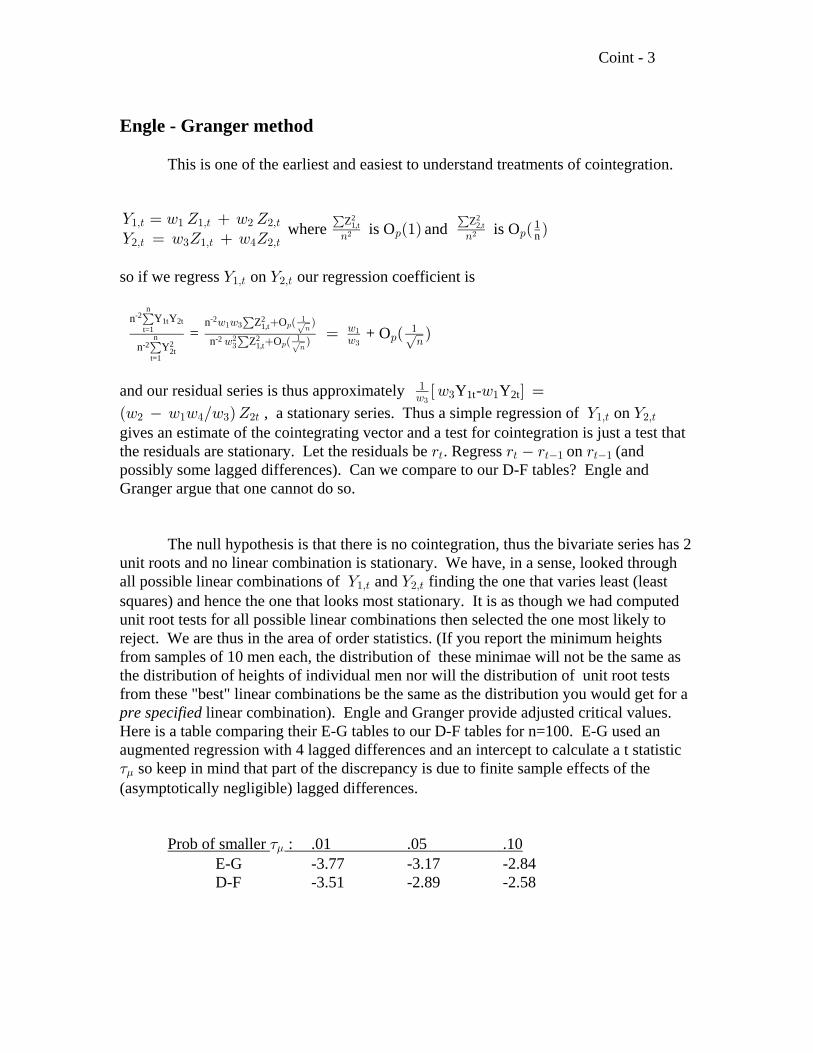
squares) and hence the one that looks most stationary. It is as though we had computedunit root tests for all possible linear combinations then selected the one most likely toreject. We are thus in the area of order statistics. (If you report the minimum heightsfrom samples of 10 men each, the distribution of these minimae will not be the same asthe distribution of heights of individual men nor will the distribution of unit root testsfrom these "best" linear combinations be the same as the distribution you would get for apre specified linear combination). Engle and Granger provide adjusted critical values.Here is a table comparing their E-G tables to our D-F tables for n=100. E-G used anaugmented regression with 4 lagged differences and an intercept to calculate a t statistic7. so keep in mind that part of the discrepancy is due to finite sample effects of the(asymptotically negligible) lagged differences.

Prob of smaller : .01 .05 .107. E-G -3.77 -3.17 -2.84 D-F -3.51 -2.89 -2.58

Coint - 4

Example:

P = cash price on delivery date, Texas steerstF = Futures pricet

(source: Ken Mathews, NCSU Ag. Econ.)Data are bimonthly Feb. '76 through Dec. '86 (60 obs.)

1. Test individual series for integration

f fP = 7.6 - 0.117 P + P (D-F) = = -2.203^t t-1 t-i

i=1

5

i-.117.053

! " 7.

f fF = 7.7 - 0.120 F + F (D-F) = = -2.228^t t-1 t-i

i=1

5

i-.120.054

! " 7.

each series is integrated, cannot reject at 10%

2. Regress F on P : F = .5861 + .9899 P , residual R^t t t t t

fR = 0.110 - .9392 R (E-G) = = -7.428t t-1-.9392.12647.

Thus, with a bit of rounding, F - 1.00 P is stationary.t t

The Engle-Granger method requires the specification of one series as the dependentvariable in the bivariate regression. Fountis and Dickey (Annals of Stat.) studydistributions for the multivariate system.

If then ] œ E] I ] ] œ M E ] I> >" > > >" >" > Ð Ñ

We show that if the true series has one unit root then the root of the least squaresestimated matrix that is closest to 0 has the same limit distribution, afterM E ^ multiplication by n, as the standard D-F tables and we suggest the use of the eigenvectorsof to estimate the cointegrating vector. The only test we can do with this is theM E ^null of one unit root versus the alternative of stationarity. Johansen's test, discussedlater, extends this in a very nice way. Our result also holds for higher dimension models,but requires the extraction of roots of the estimated characteristic polynomial.

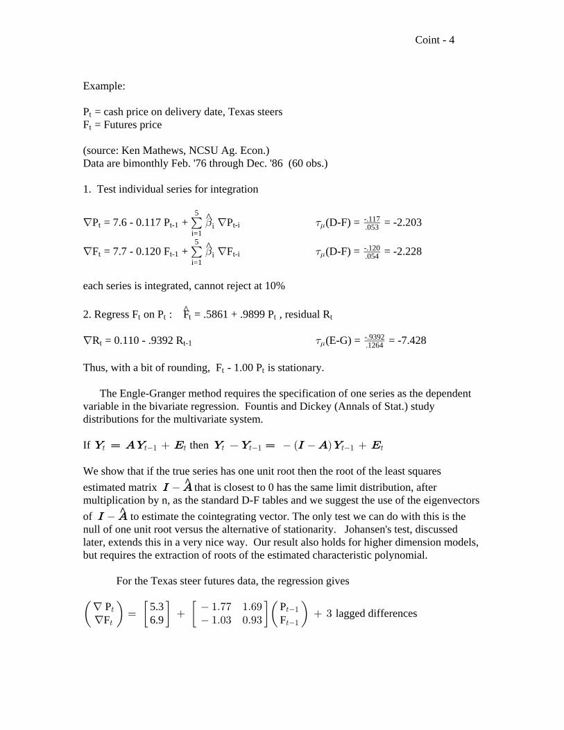
For the Texas steer futures data, the regression gives

Œ ” • ” •Œ f "Þ(( "Þ'*f "Þ!$ !Þ*$

œ $ P 5.3 PF 6.9 F lagged differences> >"

> >"

Coint - 5

where 0.54 -0.82 3.80 -4.423.63 -2.84” •” •” •-.69 0.72

"Þ(( "Þ'* "Þ!$ !Þ*$

indicating that P F is stationary. This is about .7 times the difference so .69 0.72 > tthe two methods agree that P F is stationary, as is any multiple of it.> >

Johansen's Method

This method is similar to that just illustrated but has the advantage of being ableto test for any number of unit roots. The method can be described as the application ofstandard multivariate calculations in the context of a vector autoregression, or VAR. Thetest statistics are those found in any multivariate text. Johansen's idea, like in univariateunit root tests, is to get the right for these standard calculated statistics. Thedistributionstatistics are standard, their distributions are not.

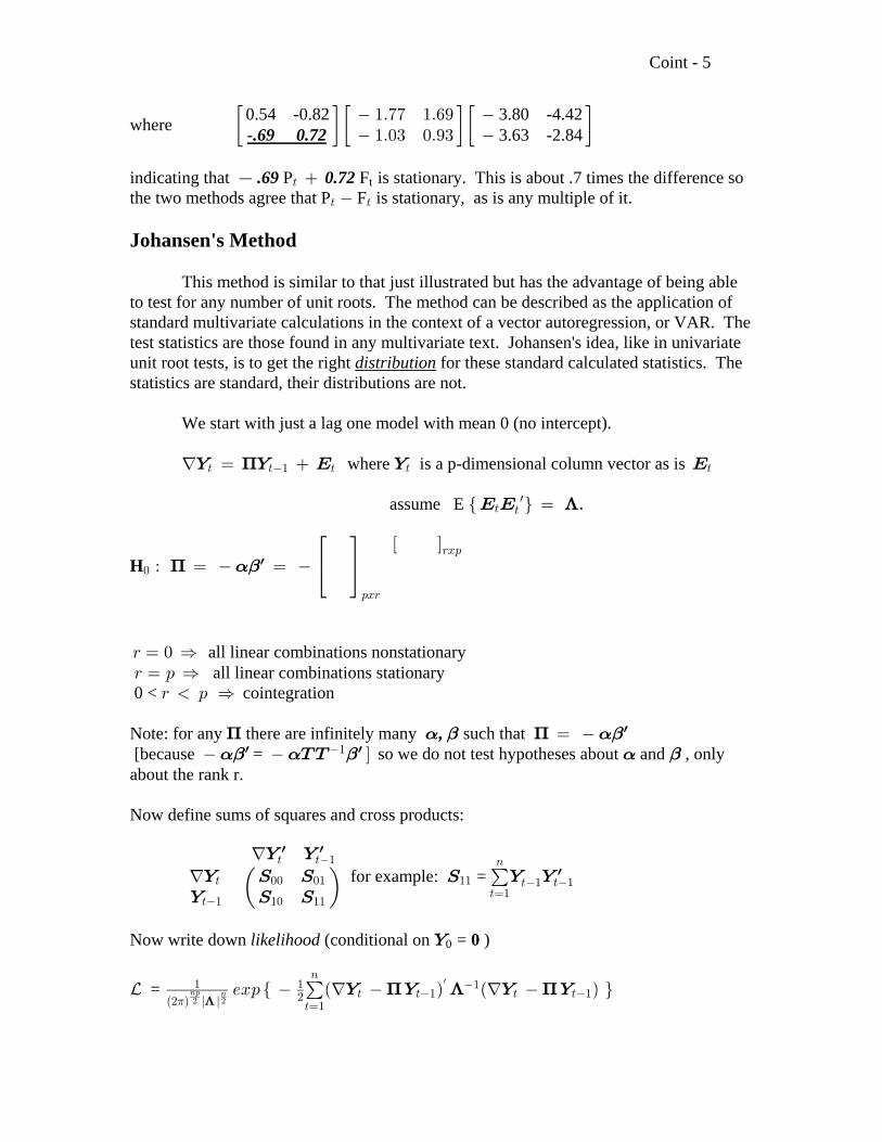
We start with just a lag one model with mean 0 (no intercept).

where is a p-dimensional column vector as is f œ ] ] I ] I> >" > > >C

assume E Ö × œI I Þ> >w A

H!

:B<

<B:

À œ œ C !"wÔ ×Õ Ø

c d

< œ ! Ê all linear combinations nonstationary all linear combinations stationary< œ : Ê 0 < cointegration< : Ê

Note: for any there are infinitely many such that C ! " C !", œ w

[because = so we do not test hypotheses about and , only Ó!" ! " ! "w wXX " about the rank r.

Now define sums of squares and cross products:

for example: = f

f

] ]

] W W] W W

W ] ]

w w

w> >"

> !! !"

>" "! ""

"">œ"

8

>" >"Π!

Now write down (conditional on = )likelihood ]0 0

_ = " "

Ð# Ñ l l #>œ"

8

> >" > >""

18:# #

8

w

A/B: Ö Ðf Ñ Ðf Ñ ×! ] ] ] ]C A C

Coint - 6

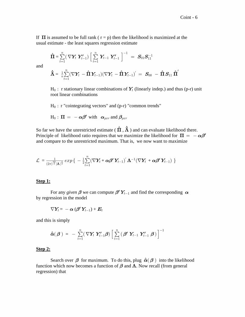
If is assumed to be full rank ( r = p) then the likelihood is maximized at theC usual estimate - the least squares regression estimate

= C ! !’ “>œ" >œ"

8 8

> >" !">" >"

""""Ðf Ñ œ] ] ] ] W Ww w

and

= ^ ^ ^ ^A C C C C^ "8>œ"

8

> >" > >" !! ""

w!Ðf ÑÐf Ñ œ ] ] ] ] W Ww

H r stationary linear combinations of (linearly indep.) and thus (p-r) unit ! >À ] root linear combinations

H r "cointegrating vectors" and (p-r) "common trends"0 À

H with and! :B< :B<À œ C !" ! "w

So far we have the unrestricted estimate ( , ) and can evaluate likelihood there.C A Principle of likelihood ratio requires that we maximize the likelihood for C !"œ w

and compare to the unrestricted maximum. That is, we now want to maximize

_ = + + " "

Ð# Ñ l l #>œ"

8

> >" > >""

18:# #

8

w

A/B: Ö Ðf Ñ Ðf Ñ ×! ] ] ] ]!" A !"w w

Step 1:

For any we can compute and find the corresponding given " " ! w ]>"

by regression in the model

= ( ) + f ] ] I> >" >! " w

and this is simply

= ! " " " "Ð Ñ Ðf Ñ Ð Ñ ! !’ “>œ" >œ"

8 8

> >">" >"

"

] ] ] ]w w w

Step 2:

Search over for maximum. To do this, plug into the likelihood^" ! " Ð Ñfunction which now becomes a function of and . Now recall (from general" Aregression) that

Coint - 7

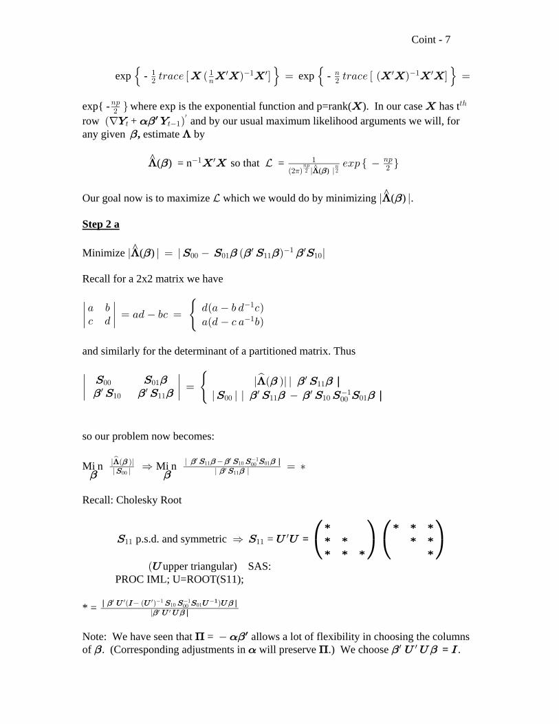
exp - exp - š › š ›1# 8 #

" 8w " w w " w><+-/ Ò Ð Ñ Ó œ ><+-/ Ò Ð Ñ Ó œ\ \ \ \ \ \ \ \

exp{ - where exp is the exponential function and p=rank( ). In our case has t8:#

>2× \ \ row + and by our usual maximum likelihood arguments we will, forÐf Ñ] ]> >"!"w w

any given estimate by" A,

( ) = n so that = A " " w "

Ð# Ñ l l

8:#\ \ _

18:# #

8A "^ ( )

/B: Ö ×

Our goal now is to maximize which we would do by minimizing ( ) .^_ l lA "

Step 2 a

Minimize ( )^l l œ l Ð Ñ lA " " " " "W W W W!! !" "" "!w " w

Recall for a 2x2 matrix we have

º º + , .Ð+ , . -Ñ- .

œ +. ,- œ+Ð. - + ,Ñ

"

"

and similarly for the determinant of a partitioned matrix. Thus

º º W WW W

W l

W W W W W l!! !"w w

"! ""

w""

!! "" "! !"w w "

!!

"" " "

A " " "

" " " "œ l Ð Ñl ls

l l l

so our problem now becomes:

Mi n Mi n " "

l Ð Ñls

l l l ll A " " " " "

" "W WW W W W l

!! ""

w w """ "! !"!!

wÊ œ ‡

Recall: Cholesky Root

p.s.d. and symmetric = W W Y Y‡ ‡ ‡ ‡‡ ‡ ‡ ‡‡ ‡ ‡ ‡

"" ""wÊ =

Î ÑÎ ÑÏ ÒÏ Ò

upper triangular) SAS:ÐY PROC IML; U=ROOT(S11);

* = l Y M Y W W W Y Y lY Y l

" "" "

w w w " ""! !"!!

w w

Ð Ð Ñ Ñl

"

Note: We have seen that = allows a lot of flexibility in choosing the columnsC !" w

of . (Corresponding adjustments in will preserve .) We choose ." ! C " "w wY Y M =

Coint - 8

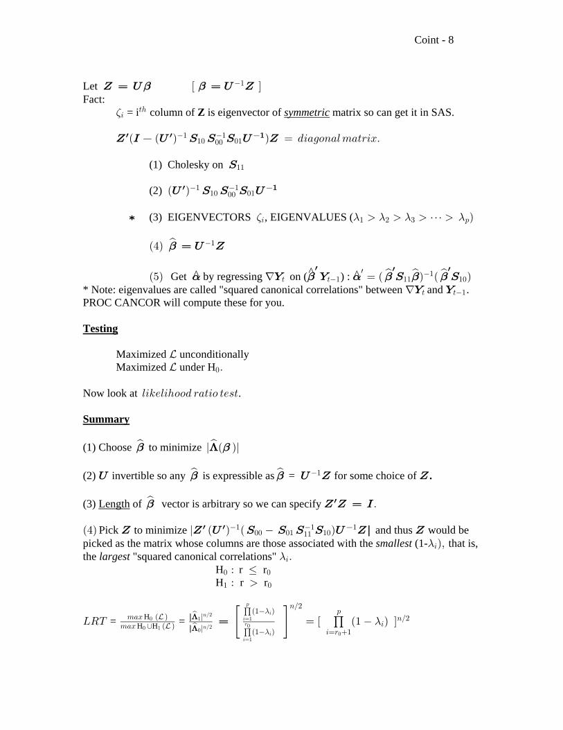
Let ^ œ Y œ Y ^" "Ò Ó"

Fact: = i column of is eigenvector of matrix so can get it in SAS.'3

>2 Z symmetric

^ M Y W W W Y ^w w "Ð Ð Ñ Ñ œ .3+198+67+><3BÞ" ""! !"!!

(1) Cholesky on W""

(2) Ð ÑY W W W Yw "" ""! !"!!

‡ (3) EIGENVECTORS , EIGENVALUES (' - - - -3 " # $ : â Ñ

Ð%Ñ s" œ Y ^"

Get by regressing on ( ) : ^ ^^Ð&Ñ f œ Ð Ñ Ð Ñs s s ! " ! " " "] ] W W> >" "" "!w "

w w w

* Note: eigenvalues are called "squared canonical correlations" between and .f] ]> >"

PROC CANCOR will compute these for you.

Testing

Maximized unconditionally_ Maximized under H_ !Þ

Now look at .635/63299. <+>39 >/=>

Summary

(1) Choose to minimize " A "s l Ð Ñls

(2) invertible so any is expressible as = for some choice of Y Y ^ ^" "s s " .

(3) of vector is arbitrary so we can specify Length "s Þ^ ^ œ Mw

Ð%Ñ l Ð Ñ Ð ÑPick to minimize and thus would be^ ^ Y W W W W Y ^l ^w w " " "!! !" "!""

picked as the matrix whose columns are those associated with the (1- that is,smallest -3Ñßthe "squared canonical correlations" largest -3Þ H r r! !À Ÿ H r r" !À

PVX œ Ò Ð" Ñ Ó = = 7+B Ð Ñ l7+B Ð Ñ

s

s l

Ð" Ñ

Ð" Ñ

8Î#

3œ< "

:

38Î#H

H H! "

! "

8Î#

!8Î#

3œ"

:

3

3œ"

<!

3 !

__

-

-

l

l

A

Aœ – — ##

# -

Coint - 9

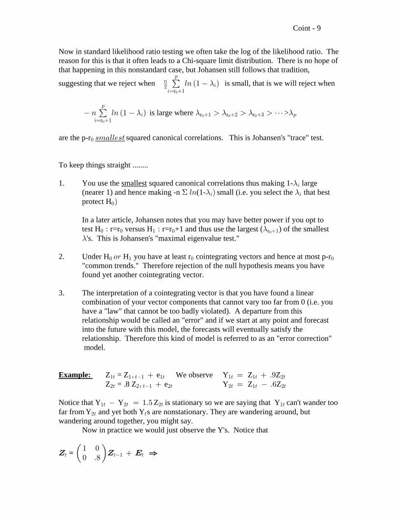
Now in standard likelihood ratio testing we often take the log of the likelihood ratio. Thereason for this is that it often leads to a Chi-square limit distribution. There is no hope ofthat happening in this nonstandard case, but Johansen still follows that tradition,

suggesting that we reject when is small, that is we will reject when8#3œ "

:

3!r!

68 Ð" Ñ-

is large where > 8 68 Ð" Ñ â!3œ "

:

3 " # $ :r

r r r!

! ! !- - - - -

are the p-r squared canonical correlations. This is Johansen's "trace" test.! =7+66/=>

To keep things straight ........

1. You use the squared canonical correlations thus making 1- largesmallest -3

(nearer 1) and hence making -n (1- small (i.e. you select the that bestD - -68 Ñ3 3

protect H!Ñ

In a later article, Johansen notes that you may have better power if you opt to test H r=r versus H r=r +1 and thus use the largest ( ) of the smallest! ! " ! "À À -r! 's. This is Johansen's "maximal eigenvalue test."-

2. Under H H you have at least r cointegrating vectors and hence at most p-r! " ! !9< "common trends." Therefore rejection of the null hypothesis means you have found yet another cointegrating vector.

3. The interpretation of a cointegrating vector is that you have found a linear combination of your vector components that cannot vary too far from 0 (i.e. you have a "law" that cannot be too badly violated). A departure from this relationship would be called an "error" and if we start at any point and forecast into the future with this model, the forecasts will eventually satisfy the relationship. Therefore this kind of model is referred to as an "error correction" model.

Example: Z = Z e We observe Y Z Z"> " >" "> "> "> #>ß œ Þ* Z = .8 Z e Y Z Z2 2 2> >" > #> "> #>ß œ Þ'

Notice that Y Y Z is stationary so we are saying that Y can't wander too"> #> #> "> œ "Þ&far from Y and yet both Y s are nonstationary. They are wandering around, but#> >

wandering around together, you might say. Now in practice we would just observe the Y's. Notice that

^ ^ I Ê> >" > = Œ " !! Þ)

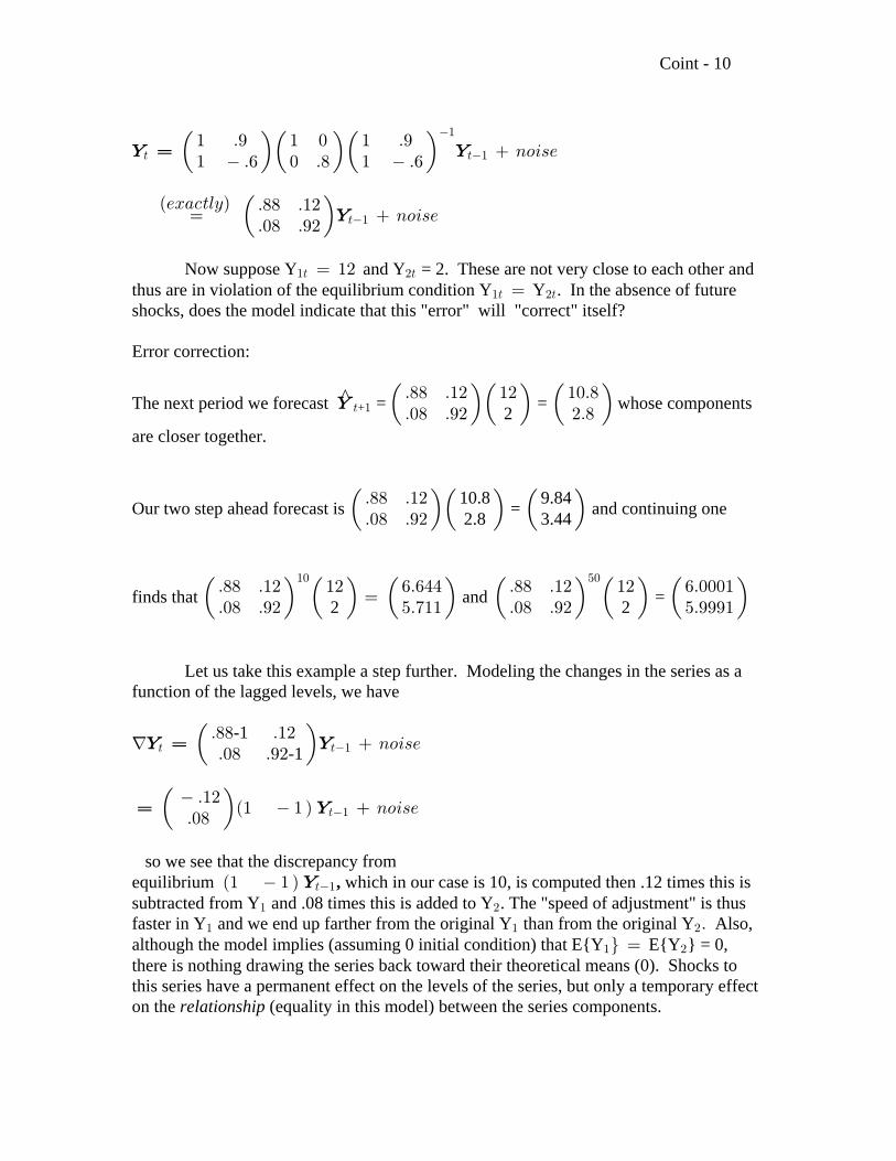
Coint - 10

] œ ]> >"

"Œ Œ Œ " Þ* " ! " Þ*" Þ' ! Þ) " Þ'

893=/

œ 893=/Ð/B+->6CÑ Þ)) Þ"#

Þ!) Þ*#Œ ]>"

Now suppose Y and Y = 2. These are not very close to each other and"> #>œ "#thus are in violation of the equilibrium condition Y Y . In the absence of future"> #>œshocks, does the model indicate that this "error" will "correct" itself?

Error correction:

The next period we forecast = = whose components^2] > "+ Œ Œ Œ Þ)) Þ"# "# "!Þ)

Þ!) Þ*# #Þ)

are closer together.

Our two step ahead forecast is = and continuing one10.8 9.842.8 3.44Œ Œ Œ Þ)) Þ"#

Þ!) Þ*#

finds that and = 2 2Œ Œ Œ Œ Œ Œ Þ)) Þ"# "# 'Þ'%% Þ)) Þ"# "# 'Þ!!!"Þ!) Þ*# &Þ("" Þ!) Þ*# &Þ***"

œ"! &!

Let us take this example a step further. Modeling the changes in the series as afunction of the lagged levels, we have

f 893=/Þ)) Þ"#Þ!) Þ*#

] œ ]> >"Œ -1-1

œ ]Œ a b Þ"#Þ!)

" 893=/ " >"

so we see that the discrepancy fromequilibrium which in our case is 10, is computed then .12 times this isa b" " ]>",subtracted from Y and .08 times this is added to Y . The "speed of adjustment" is thus" #

faster in Y and we end up farther from the original Y than from the original Y Also," " #Þalthough the model implies (assuming 0 initial condition) that E{Y E{Y } = 0," #× œthere is nothing drawing the series back toward their theoretical means (0). Shocks tothis series have a permanent effect on the levels of the series, but only a temporary effecton the (equality in this model) between the series components.relationship

Coint - 11

Remaining to do:

Q1: What are the critical values for the test? Q2: What if we have more than 1 lag? Q3: What if we include intercepts, trends, etc.

Q1. Usually the likelihood ratio test has a limit Chi-square distribution. For example aregression F test is such that 4F . Also F = t is a special case. Now% % # # #

8 8 8%Ä Ä ^_ _; 1

we have seen that the t statistic, , has a nonstandard limit distribution expressible as a7functional of Brownian Motion on [0,1]. We found:FÐ>Ñ

= 7'' '!"

! !" "# #

" "# #

"#

#FÐ>Ñ .FÐ>Ñ

Ò F Ð>Ñ .> Ó Ò F Ð>Ñ .> Ó

Ò F Ð"Ñ" Óœ

and we might thus expect Johansen's test statistic to converge to a multivariate analogueof this expression. Indeed, Johansen proved that his likelihood ratio (trace) testconverges to a variable that can be expressed as a functional of a vector valued BrownianMotion with independent components (channels) as follows (i.e. the error term hasvariance matrix I5#Ñ

LRT trace [ ] [ ] [ ] Ä Ð>Ñ . Ð>Ñ Ð>Ñ Ð>Ñ .> Ð>Ñ . Ð>Ñ_ œ ' ' '

! ! !" " "w "wF F F F F F

For a Brownian motion of dimension m = 1,2,3,4,5 (Table 1, page 239 of Johansen) hecomputes the distribution of the LRT by Monte Carlo. Empirically he notes that thesepercentiles are quite close to the percentiles of c where f=2m and c=.85-.58/f.;# #

0

We will not repeat Johansen's development of the limit distribution of the LRTbut will simply note that it is what would be expected by one familiar with the usual limitresults for F statistics and with the nonstandard limit distributions that arise with unit rootprocesses. As one might expect, the m=1 case can be derived from the distribution.7

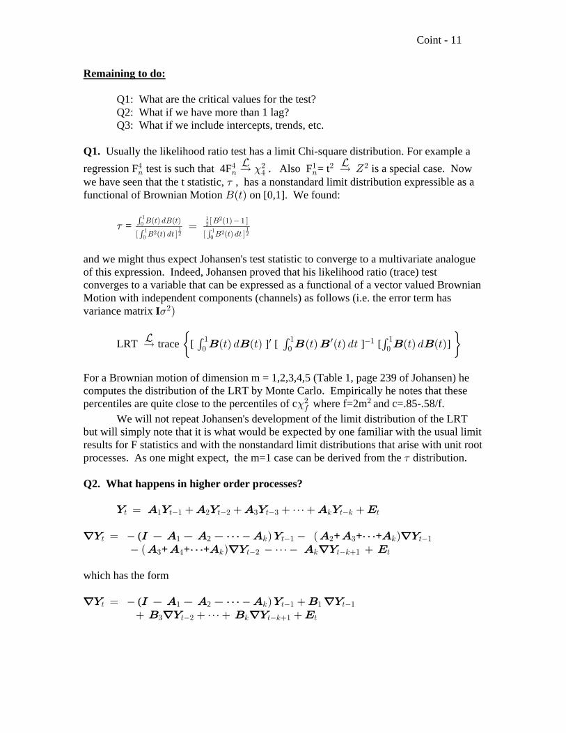
Q2. What happens in higher order processes?

] E ] E ] E ] E ] I> " >" # ># $ >$ 5 >5 >œ â

f] M E E â E ] E E â E f]> " 5 >" # $ 5 >"œ Ñ Ð Ñ ( 2 + + + Ð Ñ â E E â E f] E f] I$ % 5 ># 5 >5" >+ + +

which has the form

f] M E E â E ] F f]> " 5 >" " >"œ Ñ ( 2 â F f] F f] I$ ># 5 >5" >

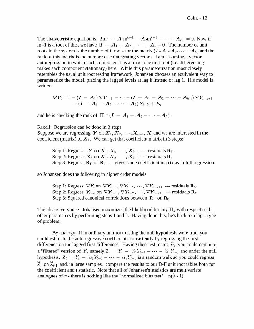
Coint - 12

The characteristic equation is | m m m Now ifM E E â E l5 5" 5#" 5 œ !Þ2

m=1 is a root of this, we have | | = 0 . The number of unitM E E â E" 52 roots in the system is the number of 0 roots for the matrix ( and theM E E â E- - -" 52 Ñrank of this matrix is the number of cointegrating vectors. I am assuming a vectorautoregression in which each component has at most one unit root (i.e. differencingmakes each component stationary) here. While this parameterization most closelyresembles the usual unit root testing framework, Johansen chooses an equivalent way toparameterize the model, placing the lagged levels at lag k instead of lag 1. His model iswritten:

f] M E ] M E E â E ]> " >" " 5 >5 "œ Ñf â Ñf ( ( 2 -1 + Ñ (M E E â E ] I" 5 >5 >2

and he is checking the rank of = ( .C M E E â E" 52 Ñ

Recall: Regression can be done in 3 steps.Suppose we are regressing on , and we are interested in the] \ ß\ ß âß\ \" # 5" 5

coefficient (matrix) of . We can get that coefficient matrix in 3 steps:\5

Step 1: Regress on --- residuals ] \ ß\ ß âß\" # 5" ]R Step 2: Regress on --- residuals R\ \ ß\ ß âß\5 " # 5" k R RStep 3: Regress on -- gives same coefficient matrix as in full regression.] k

so Johansen does the following in higher order models:

Step 1: Regress on --- residuals f f f f] ] ß ] ß âß ]> >" > # >5 " f + R Step 2: Regress on --- residuals R ] ] ß ] ß âß ]>5 >" > # >5 " 5f f f + R RStep 3: Squared canonical correlations between on ] k

The idea is very nice. Johansen maximizes the likelihood for any with respect to theC5

other parameters by performing steps 1 and 2. Having done this, he's back to a lag 1 typeof problem.

By analogy, if in ordinary unit root testing the null hypothesis were true, youcould estimate the autoregressive coefficients consistently by regressing the firstdifference on the lagged first differences. Having these estimates, , you could compute!s3

a "filtered" version of , namely Z and under the null] œ ] ] â ]s s s> > " >" : >:! !hypothesis, Z is a random walk so you could regress> > " >" : >:œ ] ] â ]! !

Z on Z and, in large samples, compare the results to our D-F unit root tables both fors s> >-1

the coefficient and t statistic. Note that all of Johansen's statistics are multivariateanalogues of - there is nothing like the "normalized bias test" n( - 1).^7 3

Coint - 13

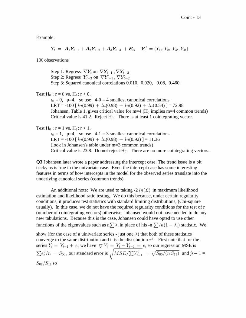
Example:

, ] E ] E ] E ] I ]> " >" # ># $ >$ > "> #> $> %>>œ œ Ð] ß ] ß ] ß ] Ñw

"!! observations

Step 1: Regress on f f f] ] ß ]> >" > #

Step 2: Regress on ] ] ß ]> >" > #3 f f

Step 3: Squared canonical correlations 0.010, 0.020, 0.08, 0.460

Test H r = vs. H : r > 0.! "À ! r = 0, p=4, so use 4-0 = 4 smallest canonical correlations.!

LRT = -100 [ (0.99) (0.98) (0.92) 0.54) ] = 72.9868 68 68 68Ð Johansen, Table 1, gives critical value for m=4 (H implies m=4 common trends)!

Critical value is 41.2. Reject H There is at least 1 cointegrating vector.!Þ

Test H r = 1 vs. H : r > 1.! "À r = 1, p=4, so use 4-1 = 3 smallest canonical correlations.!

LRT = -100 [ (0.99) (0.98) (0.92) ] = 11.3668 68 68 (look in Johansen's table under m=3 common trends) Critical value is 23.8. Do not reject H There are no more cointegrating vectors.!Þ

Q3 Johansen later wrote a paper addressing the intercept case. The trend issue is a bittricky as is true in the univariate case. Even the intercept case has some interestingfeatures in terms of how intercepts in the model for the observed series translate into theunderlying canonical series (common trends).

An additional note: We are used to taking -2 in maximum likelihood68Ð Ñ_estimation and likelihood ratio testing. We do this because, under certain regularityconditions, it produces test statistics with standard limiting distributions, (Chi-squareusually). In this case, we do not have the required regularity conditions for the test of r(number of cointegrating vectors) otherwise, Johansen would not have needed to do anynew tabulations. Because this is the case, Johansen could have opted to use otherfunctions of the eigenvalues such as n in place of his -n statistic. We! !- -3 368Ð" Ñ

show (for the case of a uinivariate series - just one ) that both of these statistics-converge to the same distribution and it is the distribution First note that for the7#Þseries we have so our regression MSE is] œ ] / ™ ] œ ] ] œ /> >" > > > >" >! !Ê È/ Î8 œ W QWIÎ ] œ W ÎÐ8W Ñ ">

#!! !! "">"

#, our standard error is and =3

W ÎW!" "" so

Coint - 14

73

œ œ " W ÎW

QWIÎ ] W ÎÐ8W Ñ

^

Ê ! È>"#

!" ""

!! ""

7È È8œ

W

W W

!"

!! ""

Now the "Cholesky root" of the univariate variable S is, of course, just and"" ""ÈW

Johansen looks at the matrix ( 1 - ) =È ÈW W"" ""W W

W W"W

!" !"

"" ""!!È ÈÈ ÈW Ñ W Þ 8"" "" 3 38( 1 - calling its eigenvalues 1- We see immediately that is just7# - -

7# so we already know its distribution (the multivariate cases are analogous). This also shows that = so if we expand Johansen's statistic, using the-3 :S Ð"Î8ÑTaylor series for expanded around , we then have68Ð" BÑ B œ !

8 68Ð" Ñ œ 8Ð 68Ð"Ñ Ð Ñ S Ð"Î8 Ñ Ñ- -3 3 :"

"!#

from which we see that 8 68Ð" Ñ œ 8 S Ð"Î8Ñ- -3 3 :

proving, as claimed, that these two statistics have the same limit distribution (of coursethere are some extra details needed for the multivariate case). Notice that for a single -these two statistics are monotone transforms of each other so even in finite samples,provided we had the right distributions, they would give exactly equivalent tests. For themore interesting multivariate case, they are the same only in the limit.

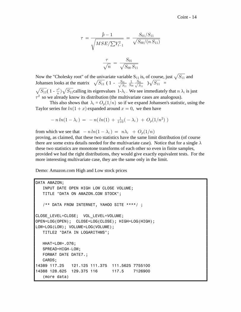
Demo: Amazon.com High and Low stock prices

DATA AMAZON; INPUT DATE OPEN HIGH LOW CLOSE VOLUME; TITLE "DATA ON AMAZON.COM STOCK";

/** DATA FROM INTERNET, YAHOO SITE ****/ ;

CLOSE_LEVEL=CLOSE; VOL_LEVEL=VOLUME;OPEN=LOG(OPEN); CLOSE=LOG(CLOSE); HIGH=LOG(HIGH);LOW=LOG(LOW); VOLUME=LOG(VOLUME); TITLE2 "DATA IN LOGARITHMS";

HHAT=LOW+.076; SPREAD=HIGH-LOW; FORMAT DATE DATE7.; CARDS;14389 117.25 121.125 111.375 111.5625 775510014388 128.625 129.375 116 117.5 7126900 (more data)

Coint - 15

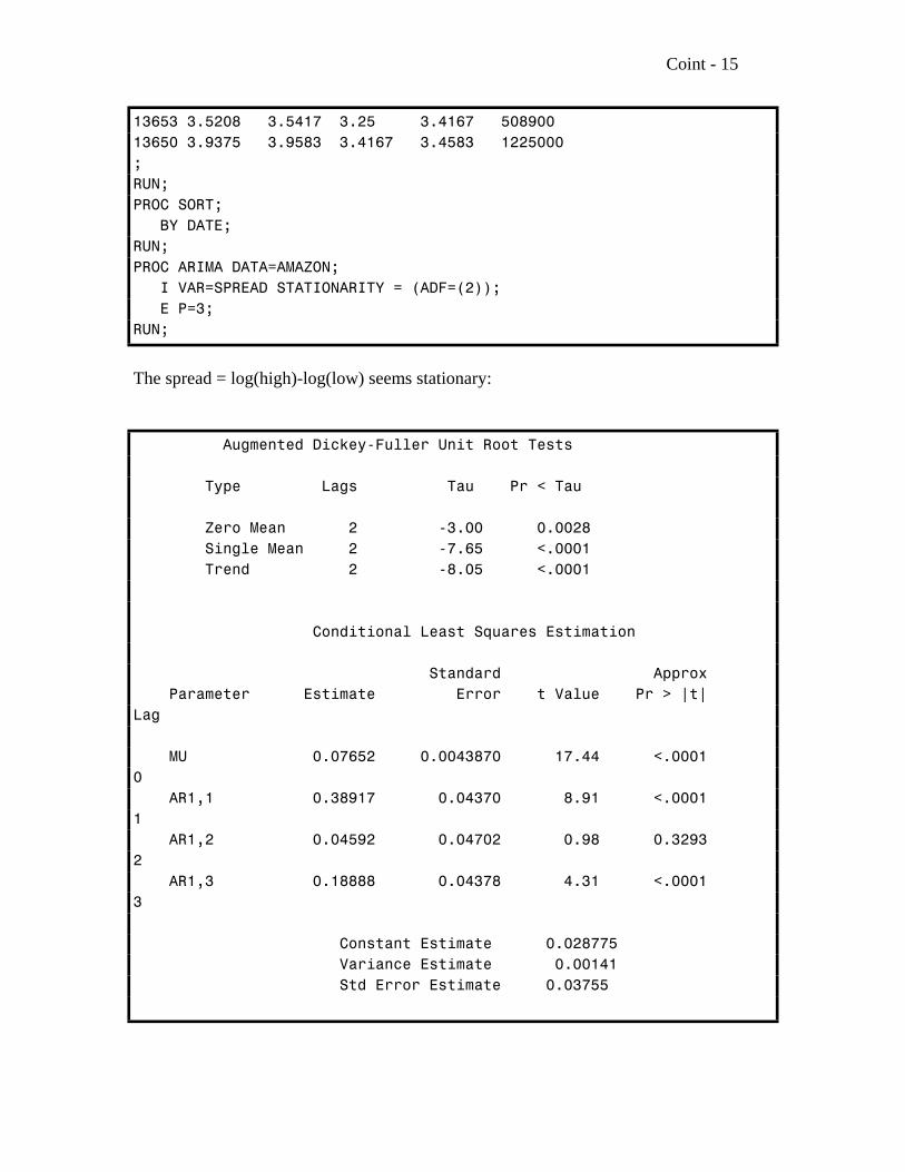
13653 3.5208 3.5417 3.25 3.4167 50890013650 3.9375 3.9583 3.4167 3.4583 1225000;RUN;PROC SORT; BY DATE;RUN;PROC ARIMA DATA=AMAZON; I VAR=SPREAD STATIONARITY = (ADF=(2)); E P=3;RUN;

The spread = log(high)-log(low) seems stationary:

Augmented Dickey-Fuller Unit Root Tests

Type Lags Tau Pr < Tau

Zero Mean 2 -3.00 0.0028 Single Mean 2 -7.65 <.0001 Trend 2 -8.05 <.0001

Conditional Least Squares Estimation

Standard Approx Parameter Estimate Error t Value Pr > |t|Lag

MU 0.07652 0.0043870 17.44 <.00010 AR1,1 0.38917 0.04370 8.91 <.00011 AR1,2 0.04592 0.04702 0.98 0.32932 AR1,3 0.18888 0.04378 4.31 <.00013

Constant Estimate 0.028775 Variance Estimate 0.00141 Std Error Estimate 0.03755

Coint - 16

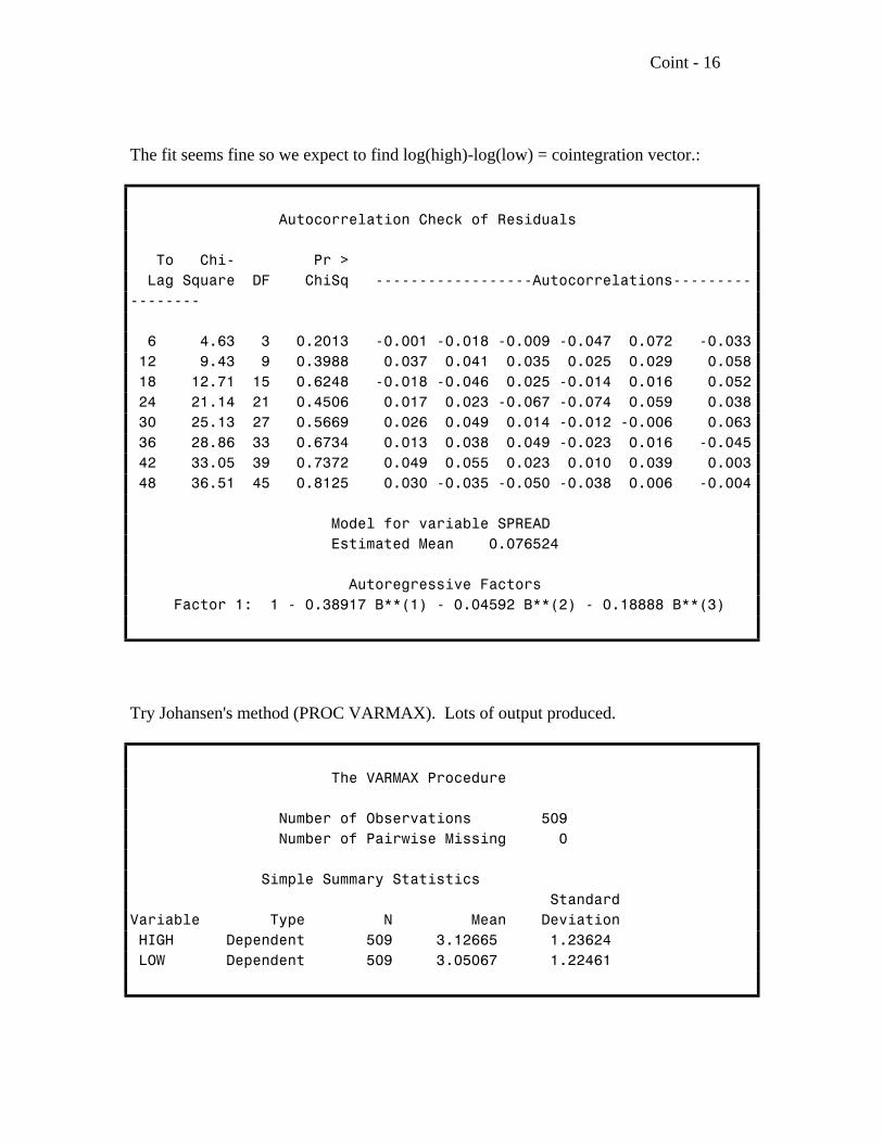
The fit seems fine so we expect to find log(high)-log(low) = cointegration vector.:

Autocorrelation Check of Residuals

To Chi- Pr > Lag Square DF ChiSq ------------------Autocorrelations-----------------

6 4.63 3 0.2013 -0.001 -0.018 -0.009 -0.047 0.072 -0.033 12 9.43 9 0.3988 0.037 0.041 0.035 0.025 0.029 0.058 18 12.71 15 0.6248 -0.018 -0.046 0.025 -0.014 0.016 0.052 24 21.14 21 0.4506 0.017 0.023 -0.067 -0.074 0.059 0.038 30 25.13 27 0.5669 0.026 0.049 0.014 -0.012 -0.006 0.063 36 28.86 33 0.6734 0.013 0.038 0.049 -0.023 0.016 -0.045 42 33.05 39 0.7372 0.049 0.055 0.023 0.010 0.039 0.003 48 36.51 45 0.8125 0.030 -0.035 -0.050 -0.038 0.006 -0.004

Model for variable SPREAD Estimated Mean 0.076524

Autoregressive Factors Factor 1: 1 - 0.38917 B**(1) - 0.04592 B**(2) - 0.18888 B**(3)

Try Johansen's method (PROC VARMAX). Lots of output produced.

The VARMAX Procedure

Number of Observations 509 Number of Pairwise Missing 0

Simple Summary Statistics StandardVariable Type N Mean Deviation HIGH Dependent 509 3.12665 1.23624 LOW Dependent 509 3.05067 1.22461

Coint - 17

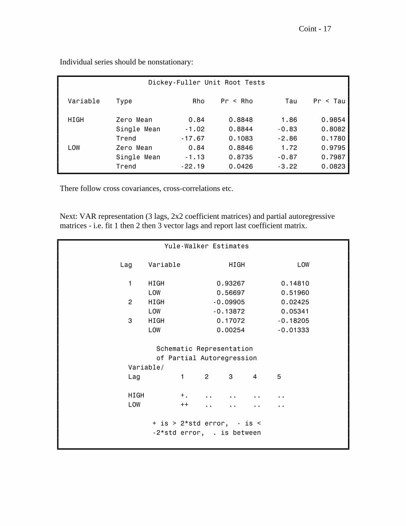
Individual series should be nonstationary:

Dickey-Fuller Unit Root Tests

Variable Type Rho Pr < Rho Tau Pr < Tau

HIGH Zero Mean 0.84 0.8848 1.86 0.9854 Single Mean -1.02 0.8844 -0.83 0.8082 Trend -17.67 0.1083 -2.86 0.1780 LOW Zero Mean 0.84 0.8846 1.72 0.9795 Single Mean -1.13 0.8735 -0.87 0.7987 Trend -22.19 0.0426 -3.22 0.0823

There follow cross covariances, cross-correlations etc.

Next: VAR representation (3 lags, 2x2 coefficient matrices) and partial autoregressivematrices - i.e. fit 1 then 2 then 3 vector lags and report last coefficient matrix.

Yule-Walker Estimates

Lag Variable HIGH LOW

1 HIGH 0.93267 0.14810 LOW 0.56697 0.51960 2 HIGH -0.09905 0.02425 LOW -0.13872 0.05341 3 HIGH 0.17072 -0.18205 LOW 0.00254 -0.01333

Schematic Representation of Partial Autoregression Variable/ Lag 1 2 3 4 5

HIGH +. .. .. .. .. LOW ++ .. .. .. ..

+ is > 2*std error, - is < -2*std error, . is between

Coint - 18

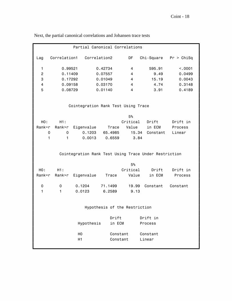
Next, the partial canonical correlations and Johansen trace tests

Partial Canonical Correlations

Lag Correlation1 Correlation2 DF Chi-Square Pr > ChiSq

1 0.99521 0.42734 4 595.91 <.0001 2 0.11409 0.07557 4 9.49 0.0499 3 0.17292 0.01049 4 15.19 0.0043 4 0.09158 0.03170 4 4.74 0.3148 5 0.08729 0.01140 4 3.91 0.4189

Cointegration Rank Test Using Trace

5% H0: H1: Critical Drift Drift in Rank=r Rank>r Eigenvalue Trace Value in ECM Process 0 0 0.1203 65.4985 15.34 Constant Linear 1 1 0.0013 0.6559 3.84

Cointegration Rank Test Using Trace Under Restriction

5% H0: H1: Critical Drift Drift in Rank=r Rank>r Eigenvalue Trace Value in ECM Process

0 0 0.1204 71.1499 19.99 Constant Constant 1 1 0.0123 6.2589 9.13

Hypothesis of the Restriction

Drift Drift in Hypothesis in ECM Process

H0 Constant Constant H1 Constant Linear

Coint - 19

The restriction is that the cointegrating vector annihilates the intercept term hence thedrift is constant in the "error correction mechanism" as well as in the process itself inanalogy to Y = 0 + Y + e . Without the restriction, an intercept appears in the ECMt t3 >"

but a linear trend appears in the process in analogy to Y = 2 + Y + e . which hast t3 >"

either a mean 2/(1- ) or drift 2 per time period depending on whether is less than 1 or3 3equal to 1. Either way, we decide there is more than 0 (Trace > Critical Value) but notmore than 1 (Trace < Critical Value).

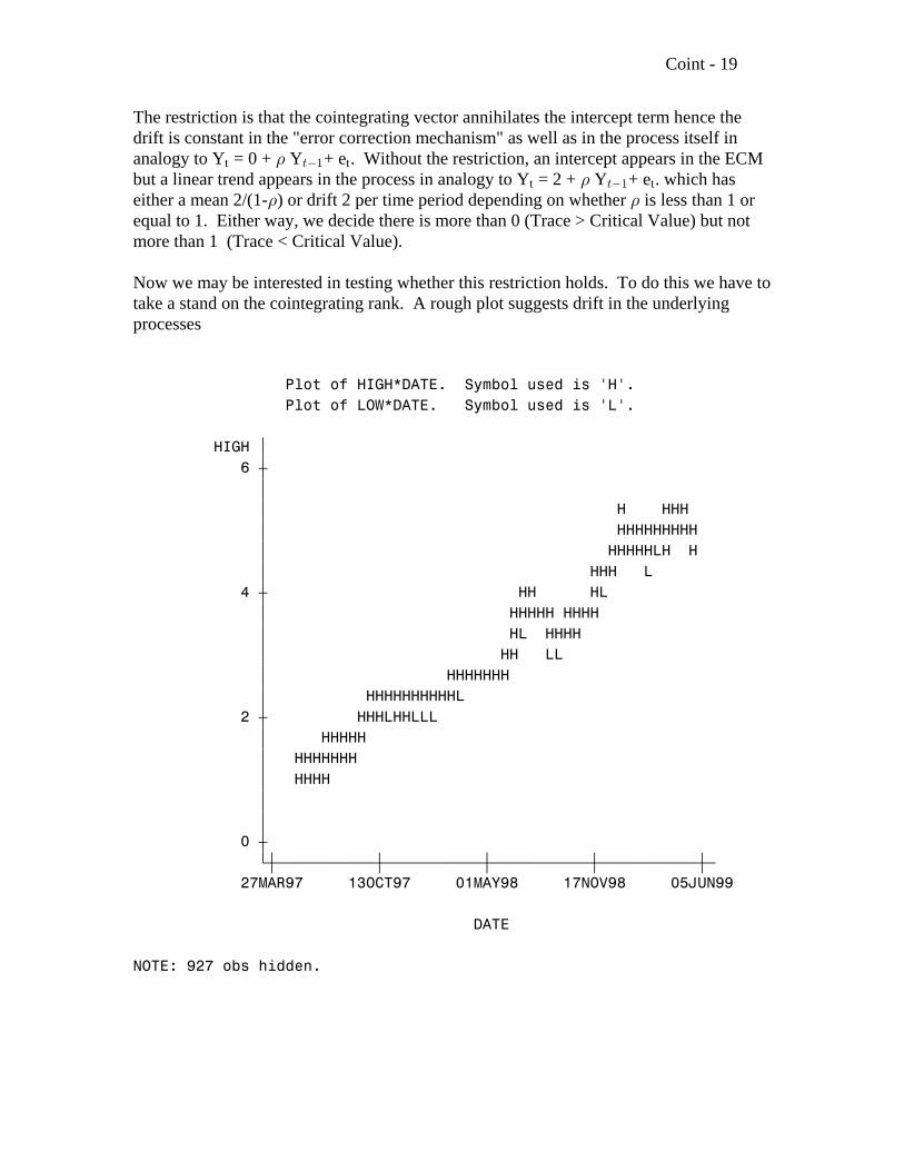
Now we may be interested in testing whether this restriction holds. To do this we have totake a stand on the cointegrating rank. A rough plot suggests drift in the underlyingprocesses

Plot of HIGH*DATE. Symbol used is 'H'. Plot of LOW*DATE. Symbol used is 'L'.

HIGH ‚ 6 ˆ ‚ ‚ H HHH ‚ HHHHHHHHH ‚ HHHHHLH H ‚ HHH L 4 ˆ HH HL ‚ HHHHH HHHH ‚ HL HHHH ‚ HH LL ‚ HHHHHHH ‚ HHHHHHHHHHL 2 ˆ HHHLHHLLL ‚ HHHHH ‚ HHHHHHH ‚ HHHH ‚ ‚ 0 ˆ Šˆƒƒƒƒƒƒƒƒƒƒƒˆƒƒƒƒƒƒƒƒƒƒƒˆƒƒƒƒƒƒƒƒƒƒƒˆƒƒƒƒƒƒƒƒƒƒƒˆƒ 27MAR97 13OCT97 01MAY98 17NOV98 05JUN99

DATE

NOTE: 927 obs hidden.

Coint - 20

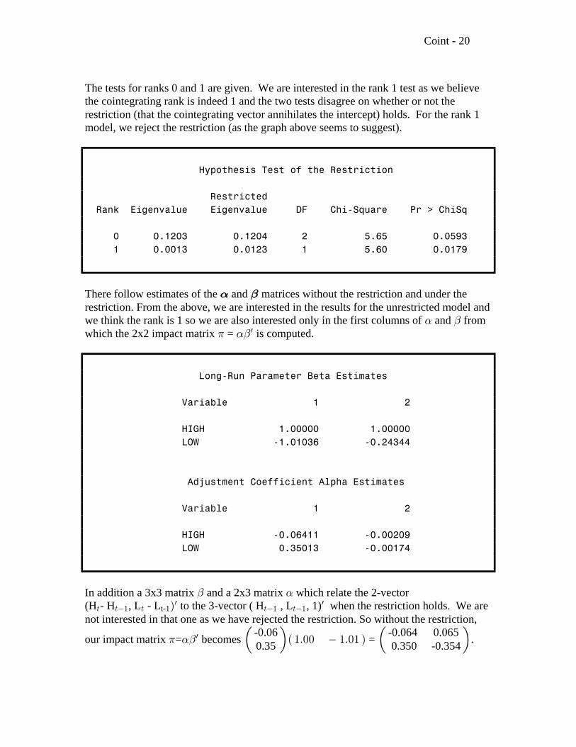
The tests for ranks 0 and 1 are given. We are interested in the rank 1 test as we believethe cointegrating rank is indeed 1 and the two tests disagree on whether or not therestriction (that the cointegrating vector annihilates the intercept) holds. For the rank 1model, we reject the restriction (as the graph above seems to suggest).

Hypothesis Test of the Restriction

Restricted Rank Eigenvalue Eigenvalue DF Chi-Square Pr > ChiSq

0 0.1203 0.1204 2 5.65 0.0593 1 0.0013 0.0123 1 5.60 0.0179

There follow estimates of the and matrices without the restriction and under the! "restriction. From the above, we are interested in the results for the unrestricted model andwe think the rank is 1 so we are also interested only in the first columns of and from! "which the 2x2 impact matrix = is computed.1 !"w

Long-Run Parameter Beta Estimates

Variable 1 2

HIGH 1.00000 1.00000 LOW -1.01036 -0.24344

Adjustment Coefficient Alpha Estimates

Variable 1 2

HIGH -0.06411 -0.00209 LOW 0.35013 -0.00174

In addition a 3x3 matrix and a 2x3 matrix which relate the 2-vector" !(H - H , L - L to the 3-vector ( H , L , 1) when the restriction holds. We are> >" > >" >"

w wt-1Ñ

not interested in that one as we have rejected the restriction. So without the restriction,

our impact matrix = becomes = .-0.06 -0.064 0.0650.35 0.350 -0.3541 !"w Œ Œ a b"Þ!! "Þ!"

Coint - 21

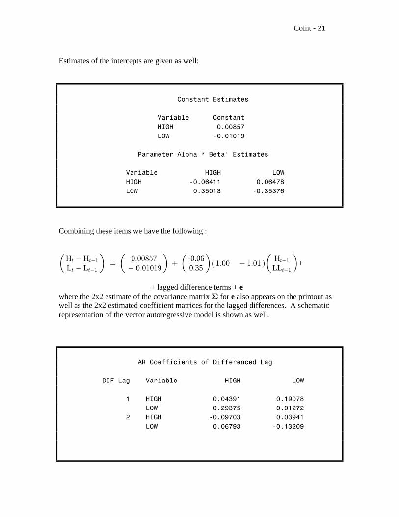
Estimates of the intercepts are given as well:

Constant Estimates

Variable Constant HIGH 0.00857 LOW -0.01019

Parameter Alpha * Beta' Estimates

Variable HIGH LOW HIGH -0.06411 0.06478 LOW 0.35013 -0.35376

Combining these items we have the following :

ΠΠΠΠa bH H -0.06 HL L 0.35 LL +> >" >"

> >" >"

!Þ!!)&( !Þ!"!"*

œ "Þ!! "Þ!"

+ lagged difference terms + ewhere the 2x2 estimate of the covariance matrix for also appears on the printout asD ewell as the 2x2 estimated coefficient matrices for the lagged differences. A schematicrepresentation of the vector autoregressive model is shown as well.

AR Coefficients of Differenced Lag

DIF Lag Variable HIGH LOW

1 HIGH 0.04391 0.19078 LOW 0.29375 0.01272 2 HIGH -0.09703 0.03941 LOW 0.06793 -0.13209

Coint - 22

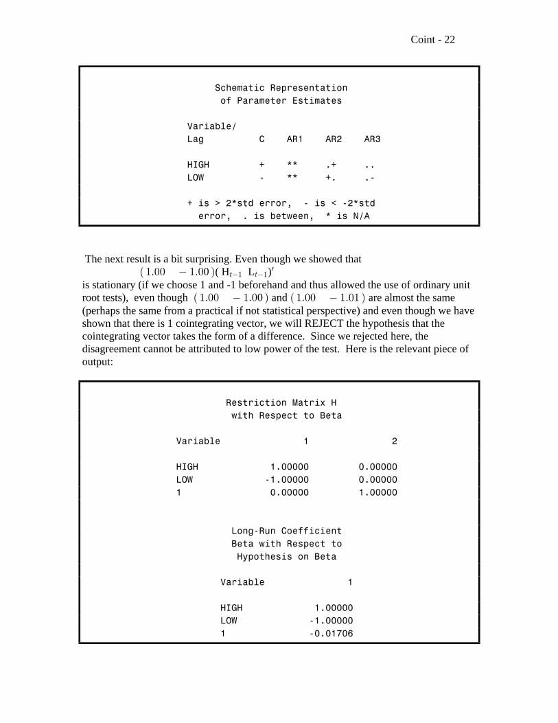
Schematic Representation of Parameter Estimates

Variable/ Lag C AR1 AR2 AR3

HIGH + ** .+ .. LOW - ** +. .-

+ is > 2*std error, - is < -2*std error, . is between, * is N/A

The next result is a bit surprising. Even though we showed that ( H L )0a b"Þ!! "Þ! >" >"

w

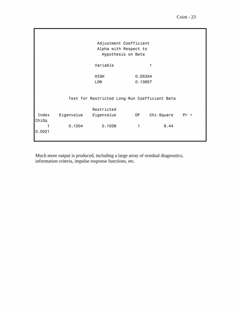
is stationary (if we choose 1 and -1 beforehand and thus allowed the use of ordinary unitroot tests), even though and are almost the same0a b a b"Þ!! "Þ! "Þ!! "Þ!"(perhaps the same from a practical if not statistical perspective) and even though we haveshown that there is 1 cointegrating vector, we will REJECT the hypothesis that thecointegrating vector takes the form of a difference. Since we rejected here, thedisagreement cannot be attributed to low power of the test. Here is the relevant piece ofoutput:

Restriction Matrix H with Respect to Beta

Variable 1 2

HIGH 1.00000 0.00000 LOW -1.00000 0.00000 1 0.00000 1.00000

Long-Run Coefficient Beta with Respect to Hypothesis on Beta

Variable 1

HIGH 1.00000 LOW -1.00000 1 -0.01706

Coint - 23

Adjustment Coefficient Alpha with Respect to Hypothesis on Beta

Variable 1

HIGH 0.05334 LOW 0.13957

Test for Restricted Long-Run Coefficient Beta

Restricted Index Eigenvalue Eigenvalue DF Chi-Square Pr >ChiSq 1 0.1204 0.1038 1 9.440.0021

Much more output is produced, including a large array of residual diagnostics,information criteria, impulse response functions, etc.