Cointegration and Regime-Switching Risk Premia in theU.S. Term Structure of Interest Rates

Peter Tillmann1

University of BonnInstitute for International Economics

Lennéstr. 37, D-53113 Bonntillmann@iiw.uni-bonn.de

first version: July 2003, this version: May 2004

Abstract: To date the cointegrating properties and the regime-switchingbehavior of the term structure are two separate strands of the literature.This paper integrates these lines of research and introduces regime shiftsinto a cointegrated VAR model. We argue that the short-run dynamics ofthe cointegrated model are likely to shift across regimes while the equilib-rium relation implied by the expectations hypothesis of the term structureis robust to regime shifts. A Markov-switching VECM approach for U.S.data outperforms a linear VECM. We find significant shifts in risk premiaand interest rate volatility. These regime shifts reflect changing inflationexpectations and shifts in monetary policy, respectively.

Keywords: term structure, expectations hypothesis, cointegration, Markov-switching, monetary policy

JEL classification: E43, E52

1Paper prepared for the 2004 North American Summer Meeting of the Econometric Society atBrown University. I thank Katrin Assenmacher-Wesche, Jens Clausen, Michael Massmann, and Man-fred J.M. Neumann as well as participants of the Deutsche Bundesbank research seminar and theHalle Wokshop "Makroökonometrie" for helpful comments on an earlier draft. All remaining errorsare mine.

1 Introduction

The information content of the term structure of interest rates has been studied in-tensively. Despite the poor empirical performance of the leading theoretical model,the expectations hypothesis, the yield curve is widely used as an indicator of mone-tary and financial conditions. According to this theory, the spread between long- andshort-term yields contains information about the future course of interest rates. Thispaper sidesteps these short-run issues and focuses on the long-run implications of theexpectations hypothesis. The hypothesis implies that long and short rates should becointegrated with cointegrating coefficients summing to zero.While the cointegration properties of the term structure are studied widely, anotherstrand of multivariate modelling analyzes regime shifts in the stochastic processesgenerating interest rates. These lines of research are largely separate strands of theliterature. Furthermore, recent research points to instability in the short-run dynamicsof cointegrating models of the term structure. These studies either assume one-timestructural shifts at predetermined dates or non-linearities governed by an observablethreshold. Thus far the cointegration properties and the Markov-switching behaviorhave not been studied jointly. Previous cointegration studies are not capable to shedlight on shifting risk premia and other regime-dependent dynamics which are likely tobe induced by shifts in monetary policy.This paper provides an unifying approach and introduces regime shifts into the coin-tegrated VAR model of the term structure. The state variable is unobservable and themodel endogenously determines the characteristics of the regimes and the break dates.Drawing on recent empirical research this paper argues that the cointegrating relationlinking long and short yields is likely to be robust to regime shifts while the short-rundynamics including the term premium and the equilibrium adjustment are dependenton the prevailing unobservable regime. Thus, this paper reconciles fluctuations instationary risk premia and error-correction parameters with the long-run equilibriumrelation implied by the expectations hypothesis. This approach offers valuable insightsinto how monetary policy regimes are reflected in term structure dynamics.We fit a Markov-switching vector error-correction model (MS-VECM) to monthlyU.S. data where the risk premium, the short-run drifts, and the loadings are regime-dependent. Given the one-to-one cointegrating relation between the three-months andvarious long rates and, thus, the stationarity of risk premia, the model is able to detectdiscrete shifts in the stochastic process corresponding to well known episodes of U.S.monetary policy.The model identifies two distinct regimes that differ mostly with respect to interestrate volatility. We find that the high-variance regime prevails during the non-borrowedreserve-targeting episode of Federal Reserve policy in 1979-1982 and other periods of

2

rising inflation expectations. Shifts to this regime imply increasing risk premia at theshort end of the term structure and decreasing risk premia for longer maturities. This isconsistent with decreasing long-run inflation expectations accompanied by increasinginflation expectations for a short horizon up to twelve months. Furthermore, theadjustment of long rates towards the equilibrium yield spread is much faster wheninterest rate volatility is high. A second regime reflects the stable post-1987 periodcharacterized by low premia for short and intermediate maturities, low volatility, andsmall expected changes in long-horizon interest rate forecasts. Thus, we supplementrecent findings of e.g. Hansen (2003) who identifies regime shifts at predetermineddates. This paper, on the contrary, lets the model endogenously choose the dates ofregime shifts and models recurrent structural change supported by a large literatureas opposed to occasional structural instability.The plan of the paper is the following: The next section derives the cointegratingproperties from a simple exposition of the expectations hypothesis and provides abrief review of the literature. Section three sets up a linear VECM and tests thecointegrating properties for U.S. data while section four proposes a regime switchingVECM approach and interprets the findings. Section five finally concludes.

2 Information in the term structure of interest rates

This section gives a brief overview of recent research on the equilibrium relationshipbetween interest rates of different maturity. We first derive the cointegrating propertiesimplied by a standard formulation of the expectations hypothesis of the term struc-ture and then survey the existing evidence with a special focus on the regime-shiftingbehavior of interest rates and, hence, the term structure.

2.1 Cointegration and the expectations hypothesis

The expectations hypothesis of the term structure of interest rates implies a stable one-to-one relationship between short and long rates. Suppose an n-period pure discountbond yields Rt(n) while the forward rate Ft(n) is the yield from contracting at time tto buy a one period pure discount bond at time t+n which matures at time t+n+1.Then it holds that Ft(0) = Rt(1). The Fisher-Hicks formula gives

Rt(n) =1

n

n−1Xj=0

Ft(j) (1)

The expectations hypothesis says that

Ft(n) = Et (Rt+n(1)) + θ (n) (2)

3

where θ (n) is the risk premium and Et denotes the expectations operator based oninformation at time t. Substituting gives

Rt(n) =1

n

n−1Xj=0

(Et (Rt+j(1)) + θ (j))

(3)

=1

n

n−1Xj=0

Et (Rt+j(1))

+ φ (n)

with φ (n) = 1n

Pn−1j=0 θ (j) as the average risk premium. The pure expectations hy-

pothesis requires φ (n) = 0, while weaker versions restrict this term to be constant orstationary. This no-arbitrage condition says that the long rate equals the weightedaverage of the expected short rates. The term premium measures the additional gainfrom holding long-term bonds relative to rolling-over one-period bonds. Using theidentity

Et(Rt+j(1)) =

jXi=1

Et (∆Rt+i(1)) +Rt(1) (4)

and rearranging results in

Rt(n)−Rt(1) = 1

n

n−1Xj=1

jXi=1

Et (∆Rt+i(1))

+ φ (n) (5)

where ∆ is the difference operator. Assuming that Rt(1) and Rt(n) are integratedof order one, I(1), it follows that the right-hand side of (5) is stationary (given astationary risk premium). Thus, the linear combination Rt(n)−Rt(1) is stationary. Inother words, the vector xt = [Rt(n), Rt(1)]

0 is cointegrated with a cointegration vectorβ = (1,−1)0. The necessary condition for the expectations condition to hold is thatwe can impose the restriction β = (1,−1)0 onto the yield spread. In this case the termpremium is stationary.The risk premium φ (n) will later be reflected as a constant in the cointegrating space.Note that the relation described by (5) holds for any pair (n, 1). In the following weassume that the short rate is the three-months interest rate Rt(3) and analyze thespread Rt(n)−Rt(3) for n ∈ {6, 12, 36, 60, 120} months.The seminal work of Campbell and Shiller (1987) shows that present value modelsimply cointegration. They find a cointegrating vector of (1,−1)0 as required by theexpectations hypothesis. These cointegrating properties of the term structure are alsoexamined by Hall, Anderson, and Granger (1992) in a VECM for twelve variables.They find a cointegration vector consistent with the theory. Shea (1992) examinespairwise cointegration relations and finds mixed evidence. Engsted and Tanggaard

4

(1994) find support for the long-run implications of the expectations hypothesis forthe U.S. while Cuthbertson (1996) provides support from UK interbank data.Although these studies suggest that the term premium is stationary, a large bodyof research initiated by Engle, Lilien, and Robins (1987) confirms the time-varyingnature of risk premia in excess holding yields that increase with volatility. Hence, amain point of term structure modelling is to quantify the size and the behavior of theterm premium. This paper supplements existing cointegration studies by showing thedynamics of the term premium given its stationarity.

2.2 Regime shifts in the term structure

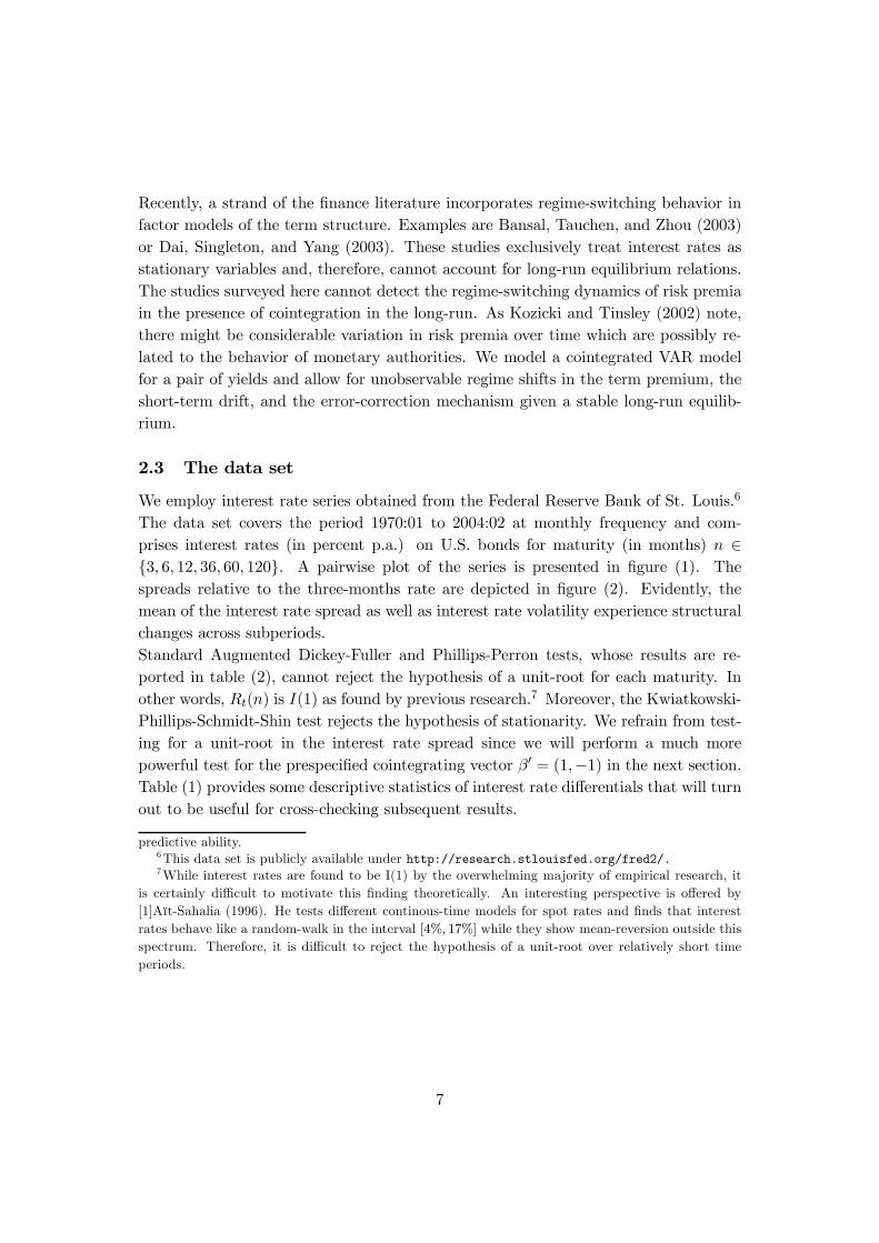
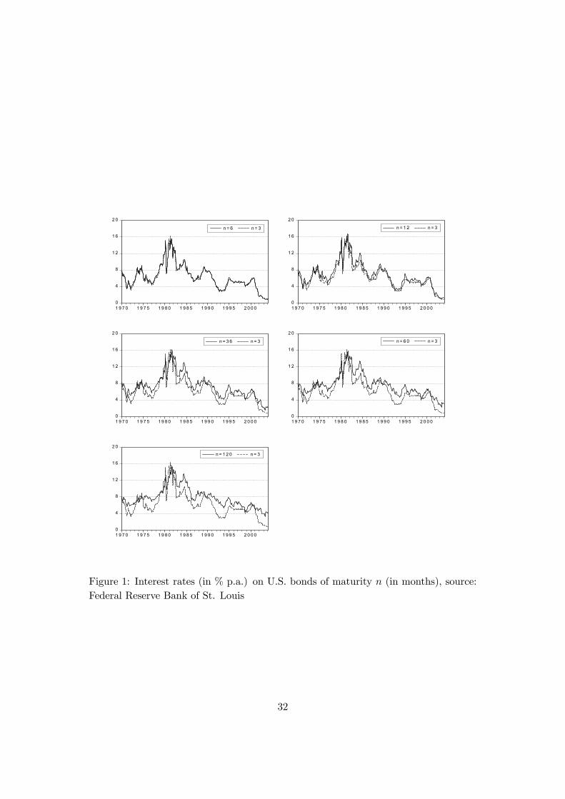
A large strand of the literature argues that regime shifts in monetary policy translateinto regime shifts in interest rates and, thus, into regime-dependent behavior of theterm structure. The change in the operating procedures of the Federal Reserve between1979 and 1982 are frequently seen as a potential source of shifts in the term structuremotivating many Markov-switching applications. In 1979 the Federal Reserve movedfrom interest rate targeting to money growth targeting and allowed the interest rate tofluctuate freely. This shift resulted in dramatically higher and more volatile short-terminterest rates as can be seen from figure (1) and induced a change in the stochasticprocess of the entire term structure.Sola and Driffill (1994) estimate a vector autoregression (VAR) for three and six monthsrates and allow for Markov regime shifts. They find their multivariate model to be moreefficient than Hamilton’s (1988) original regime-switching contribution. Regime shiftsoccur between 1979 and 1982 during the monetary targeting intermezzo of the FederalReserve.2 Similar studies by Kugler (1996) and Engsted and Nyholm (2000), amongmany others, for Swiss and Danish data support the regime-dependent behavior of theterm structure and provide mixed results on the validity of the expectations hypothesis.The regime-dependent nature of term structure dynamics is a stylized fact.3 However,the aforementioned studies model shifts in interest rates in a stationary VAR systemin first differences since interest rates are likely to be I(1). Thus far the cointegratingproperties and the regime shifts are treated separately.4 This paper, on the contrary,

2Fuhrer (1996) shows that minor shifts in the coefficients of the central bank’s reaction functioncan significantly affect the behavior and the information content of the term structure. Cogley (2003)uses a bivariate Bayesian VAR with interest rates of different maturity and allows for drifting condi-tional means and stochastic volatility of the innovation variance to study the changing nature of termstructure dynamics.

3Additional evidence on the regime-dependent stochastic processes determining interest rates ispresented in Ang and Bekaert (2002), Bekaert, Hodrick, and Marshall (2001), and Gray (1996).

4The short-term predictive power of the term structure for future interest rates may be severelyimpaired by the existence of a peso problem when the sample moments do not coincide with populationmoments taken into account by rational agents. Peso problems provide an additional motivation to

5

proposes a joint modelling approach.Another line of research studies potential instability in cointegrated systems and ap-plies various testing procedures to term structure data. Hansen (1992a) develops aLagrange-Multiplier test for parameter instability and finds a stable one-to-one re-lationship. Hansen and Johansen (1999) elaborate a recursive maximum likelihoodprocedure that employs the time paths of the eigenvalues to analyze the stability of aVECM. This test confirms the constancy of the cointegrating vector for a set of fourU.S. interest rates. Hansen (2003) generalizes Johansen’s (1988) maximum likelihoodprocedure to allow for structural change. He finds significant changes in the short-rundynamics of the VECM in September 1979 and October 1982 but cannot reject thehypothesis of a stable long-run equilibrium. The risk premium, the variance-covariancematrix, and the adjustment coefficients are subject to discrete shifts while the cointe-grating vector is unaffected by shifts in monetary policy. This econometric exercise,however, requires the dates of the regime shifts to be known in advance and tests formultiple breaks as compared to recurrent shifts between a predetermined number ofdistinct regimes. The attractiveness of the Markov-switching approach, on the con-trary, is that the model endogenously separates regimes arising from a probabilisticprocess and dates their shifts without imposing a priori break dates.Related studies argue that the term structure is characterized by non-linear and asym-metric adjustment towards the equilibrium in the sense that a regime-shift occurs oncethe spread exceeds a threshold. Hansen and Seo (2002) and Seo (2003) develop athreshold cointegration model and find evidence of non-linear mean reversion. Whilethe state variable is observable in their case, this paper puts forward a regime-switchingmodel with an unobservable state variable. Moreover, while these studies model non-linearity depending on the size and the sign of deviations from equilibrium, the modelpresented in this paper exhibits non-linearity over time.It appears as a consensus view that the long-run cointegrating properties of the termstructure are robust to regime shifts. In fact, Engsted and Tanggaard (1994, p. 175)argue that "the one-to-one relationship between long- and short-term rates given bythe expectations hypothesis is not in any way dependent on the specific process gener-ating short-term rates. If the expectations hypothesis is true, we therefore expect thecointegration implications to hold for the whole period and not just in periods of stablemonetary policy". Hence, the low frequency properties of the term structure (i.e. thecointegrating vector) should be robust to regime shifts while the high frequency prop-erties (i.e. the risk premium and the short-run dynamics) are likely to reflect regimeshifts. This approach is pursued in the remainder of this paper.5

employ state-dependent regression models, see Bekaert, Hodrick, and Marshall (2001).5 In related work, Gutiérrez and Vázquez (2003) analyse how the predictive content of the spread

for short rate changes has changed over the post-war period. They find one regime with a random-walk behavior of the short rate and another with a high and volatile rate where the spread has some

6

Recently, a strand of the finance literature incorporates regime-switching behavior infactor models of the term structure. Examples are Bansal, Tauchen, and Zhou (2003)or Dai, Singleton, and Yang (2003). These studies exclusively treat interest rates asstationary variables and, therefore, cannot account for long-run equilibrium relations.The studies surveyed here cannot detect the regime-switching dynamics of risk premiain the presence of cointegration in the long-run. As Kozicki and Tinsley (2002) note,there might be considerable variation in risk premia over time which are possibly re-lated to the behavior of monetary authorities. We model a cointegrated VAR modelfor a pair of yields and allow for unobservable regime shifts in the term premium, theshort-term drift, and the error-correction mechanism given a stable long-run equilib-rium.

2.3 The data set

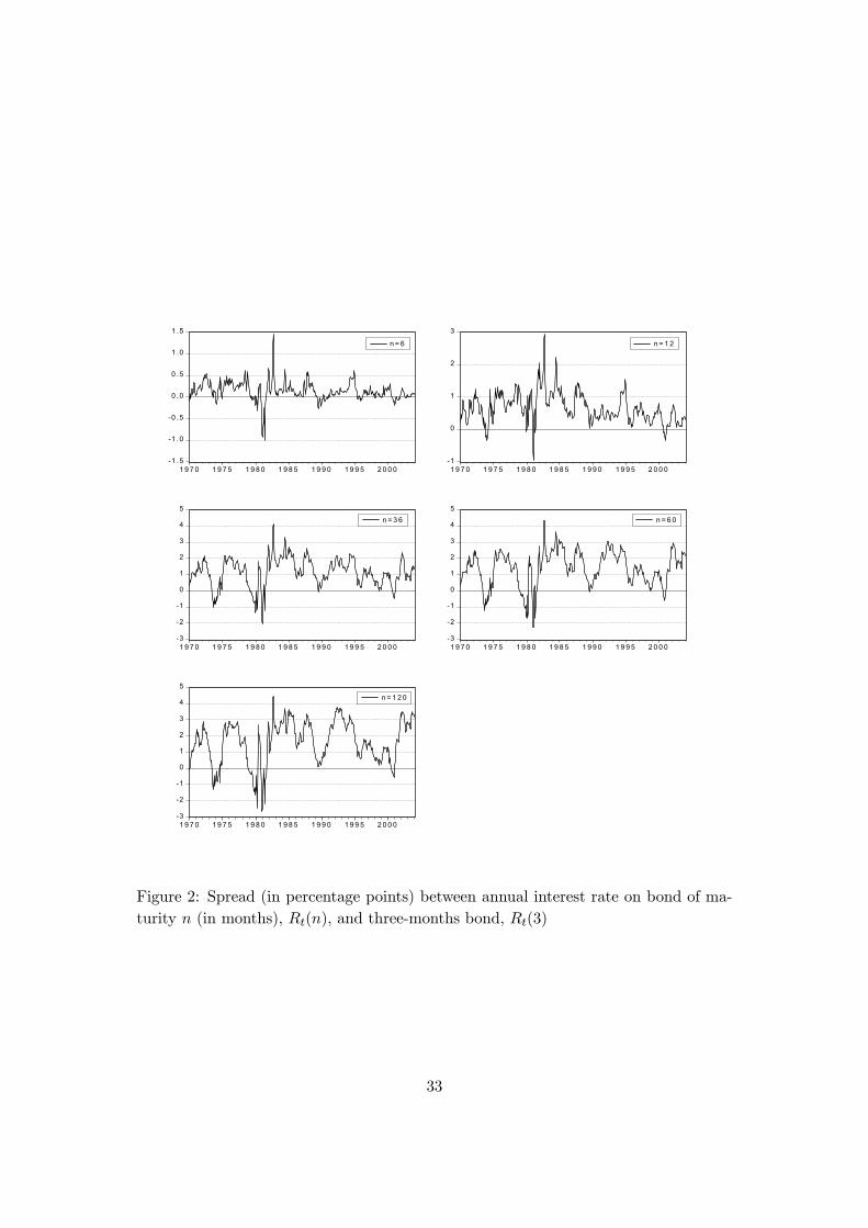
We employ interest rate series obtained from the Federal Reserve Bank of St. Louis.6

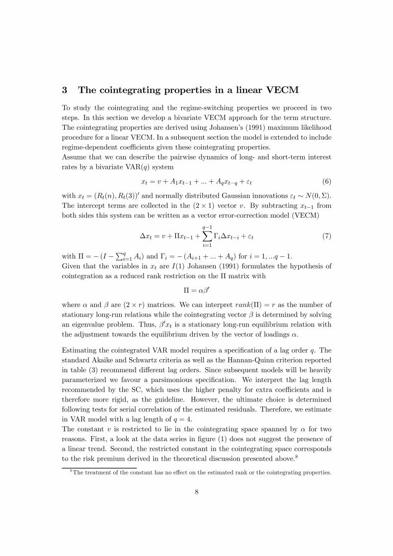
The data set covers the period 1970:01 to 2004:02 at monthly frequency and com-prises interest rates (in percent p.a.) on U.S. bonds for maturity (in months) n ∈{3, 6, 12, 36, 60, 120}. A pairwise plot of the series is presented in figure (1). Thespreads relative to the three-months rate are depicted in figure (2). Evidently, themean of the interest rate spread as well as interest rate volatility experience structuralchanges across subperiods.Standard Augmented Dickey-Fuller and Phillips-Perron tests, whose results are re-ported in table (2), cannot reject the hypothesis of a unit-root for each maturity. Inother words, Rt(n) is I(1) as found by previous research.7 Moreover, the Kwiatkowski-Phillips-Schmidt-Shin test rejects the hypothesis of stationarity. We refrain from test-ing for a unit-root in the interest rate spread since we will perform a much morepowerful test for the prespecified cointegrating vector β0 = (1,−1) in the next section.Table (1) provides some descriptive statistics of interest rate differentials that will turnout to be useful for cross-checking subsequent results.

predictive ability.6This data set is publicly available under http://research.stlouisfed.org/fred2/.7While interest rates are found to be I(1) by the overwhelming majority of empirical research, it

is certainly difficult to motivate this finding theoretically. An interesting perspective is offered by[1]Aït-Sahalia (1996). He tests different continous-time models for spot rates and finds that interestrates behave like a random-walk in the interval [4%, 17%] while they show mean-reversion outside thisspectrum. Therefore, it is difficult to reject the hypothesis of a unit-root over relatively short timeperiods.

7

3 The cointegrating properties in a linear VECM

To study the cointegrating and the regime-switching properties we proceed in twosteps. In this section we develop a bivariate VECM approach for the term structure.The cointegrating properties are derived using Johansen’s (1991) maximum likelihoodprocedure for a linear VECM. In a subsequent section the model is extended to includeregime-dependent coefficients given these cointegrating properties.Assume that we can describe the pairwise dynamics of long- and short-term interestrates by a bivariate VAR(q) system

xt = v +A1xt−1 + ...+Aqxt−q + εt (6)

with xt = (Rt(n), Rt(3))0 and normally distributed Gaussian innovations εt ∼ N(0,Σ).The intercept terms are collected in the (2× 1) vector v. By subtracting xt−1 fromboth sides this system can be written as a vector error-correction model (VECM)

∆xt = v +Πxt−1 +q−1Xi=1

Γi∆xt−i + εt (7)

with Π = − (I −Pqi=1Ai) and Γi = − (Ai+1 + ...+Aq) for i = 1, ...q − 1.

Given that the variables in xt are I(1) Johansen (1991) formulates the hypothesis ofcointegration as a reduced rank restriction on the Π matrix with

Π = αβ0

where α and β are (2× r) matrices. We can interpret rank(Π) = r as the number ofstationary long-run relations while the cointegrating vector β is determined by solvingan eigenvalue problem. Thus, β0xt is a stationary long-run equilibrium relation withthe adjustment towards the equilibrium driven by the vector of loadings α.

Estimating the cointegrated VAR model requires a specification of a lag order q. Thestandard Akaike and Schwartz criteria as well as the Hannan-Quinn criterion reportedin table (3) recommend different lag orders. Since subsequent models will be heavilyparameterized we favour a parsimonious specification. We interpret the lag lengthrecommended by the SC, which uses the higher penalty for extra coefficients and istherefore more rigid, as the guideline. However, the ultimate choice is determinedfollowing tests for serial correlation of the estimated residuals. Therefore, we estimatein VAR model with a lag length of q = 4.The constant v is restricted to lie in the cointegrating space spanned by α for tworeasons. First, a look at the data series in figure (1) does not suggest the presence ofa linear trend. Second, the restricted constant in the cointegrating space correspondsto the risk premium derived in the theoretical discussion presented above.8

8The treatment of the constant has no effect on the estimated rank or the cointegrating properties.

8

The results of Johansen’s (1991) maximum likelihood estimation of the Π = αβ0 ma-trix are presented in table (4). For each pair of maturities x0t = [Rt(n), Rt(3)] the tracetest and the maximum eigenvalue test cannot reject the hypothesis of r ≤ 1 whilethe hypothesis of r = 0 is clearly rejected in all cases. The strength of the cointe-grating property weakens with maturity as reflected by the maximum eigenvalue λmax

which decreases as maturity n increases. Thus, we find strong evidence in favor ofcointegration and can set r̂ = 1 in subsequent estimations.In addition, the cointegration test developed by Horvath and Watson (1995) supportsthe presence of a cointegrating relation. Moreover, this test, which evaluates thehypothesis of no cointegration against the alternative of a cointegrating vector withunit coefficients, supports the prediction from the expectations hypothesis. Note thatthis test amounts to a standard Likelihood-Ratio test for the presence of the candidateerror-correction terms in a first difference VAR and is more powerful than conventionalunit-root tests applied to the interest rate spread.To test the implications of the expectations hypothesis we impose restrictions ontothe cointegrating vector β = (βlong,βshort)

0. In table (5) we normalize βlong = 1

and impose the restriction β0 = (1,−1) on the system. This restriction cannot berejected in almost any of the scenarios using Likelihood Ratio tests. The restriction isrejected for the [Rt(12), Rt(3)] pair. Given the results of the aforementioned powerfulHorvath-Watson test, however, we proceed as if the unitary coefficient were accepted.Thus, we find strong support for the cointegrating implications of the expectationshypothesis: long and short rates cointegrate with a cointegrating vector β0 = (1,−1).The stationary linear combination indeed corresponds to the spread implied by theexpectations hypothesis.While at the short end of the term structure the long-run equilibrium is given byRt(6) − Rt(3) = 0.15, the constant grows to 1.96 for the widest yield spread. Asdiscussed earlier, this intercept in the cointegrating equation can be interpreted as arisk premium embedded in long rates. The risk premium increases monotonically withmaturity.The adjustment of ∆xt towards the long-run equilibrium is described by the vectorof loading coefficients α = (αlong,αshort)

0. In theory, both adjustment parametersshould be positive because a larger spread β0xt means that long rates earn a higherinterest rate, so long bonds must eventually depreciate and the long rate must rise toequilibrate the system. Since the expectations hypothesis claims that the long rate isan average of future short rates, the short rate is also expected to rise. However, wefind this prediction to be satisfied only at the short end of the term structure, see table(5). In all other models, αlong < 0 and αshort > 0. This pattern is inconsistent with theshort-run implications of the expectations hypothesis but is in line with the existingempirical evidence. Campbell and Shiller (1991, p. 496) argue: "In a nutshell, when

9

the spread is high the long rate tends to fall and the short rate tends to rise". Testingfor weak exogeneity of either interest rate series amounts to restricting the respectiveadjustment coefficient to zero. In all but one case αshort = 0 can be rejected whileαlong = 0 cannot be rejected at the short end only. Thus, some of the equilibriumadjustment occurs through movements in the short rate and not the long rate. This issomewhat surprising given that fact that movements in the short rate should closelyreflect monetary policy set autonomously.Before estimating the regime-switching model we test whether the residuals from thelinear VECM exhibit non-linearity in the sense of deviation from the assumed IIDdistribution. For this purpose the Brock-Dechert-Scheinkman (BDS) diagnostic testis applied which tests the null hypothesis of linearity against an unspecified non-linearalternative.9 The test statistic derived by Brock et al. (1996) is asymptotically normaland is reported in table (6) for alternative parameter constellations. For all VECMspecifications the hypothesis of linearity is rejected at highest levels of significance.Thus, it seems that the linear VECM fails to capture non-linearities prevailing in thetrue data-generating process.Since we cannot reject the long-run implications of the expectations hypothesis, we nowturn to the analysis of regime shifts in the short-run dynamics given this estimatedlong-run equilibrium relationship.

4 A Markov-switching VECM

In this section a Markov-switching VECM is proposed that generalizes the modeldescribed by (7) to account for regime shifts. In other words, the model is piecewiselinear in each regime but non-linear across regimes. If the number of regimes is setto unity, the model collapses to (7). Clarida et al. (2003) and Sarno, Thornton,and Valente (2002) use a similar approach, although for different purposes. Theyare primarily interested in the forecasting properties of the MS-VECM and do notdisentangle regime-shifting parameters to gain information about the behavior of theterm premia.We model regime shifts given the one-to-one equilibrium relationship found in the pre-vious section. Certainly, the well-established framework developed by Johansen (1991)models long-term properties for linear systems. However, recent work by Saikkonen andLuukkonen (1997) shows that these procedures originally developed for finite GaussianVAR systems can be employed when the data are generated by an infinite non-Gaussian

9Psaradakis and Spagnolo (2002) compare the relative performance of portmanteau-type tests todetect nonlinearity generated by Markov regime-switching. They conclude that the BDS test is gen-erally very powerful.

10

VAR.10 Thus we follow the considerations of Krolzig (1997) and the empirical work byKrolzig, Marcellino, and Mizon (2002), Sarno, Thornton, and Valente (2002), Claridaet al. (2003), and Francis and Owyang (2003) and proceed in two steps by impos-ing the cointegrating properties derived in the linear model onto the regime-switchingmodel.

4.1 Model specification

Suppose that the system describing short and long rates is driven by an unobservablediscrete state variable st = m with two possible regimes m ∈ {1, 2}

∆xt = v(st) +Π (st)xt−1 +q−1Xi=1

Γi (st)∆xt−i + εt (8)

εt ∼ N(0,Σ (st))

In contrast to the model in (7), the vector of intercept terms v(st), the error-correctionterms α (st), the dynamics of the stationary part Γi (st), and the variance-covarianceterms Σ (st) of the innovations of this VECM are conditioned on the realization of thestate variable. Note that β is regime-independent. Given the long-run equilibriumrelationship we can safely impose β0 = (1,−1) derived in the previous section. Fur-thermore, we can decompose the regime-dependent vector of intercepts into one partentering the cointegrating space and one part affecting the short-run dynamics ∆xt

∆xt − δ (st) = α (st)£β0xt−1 − µ (st)

¤+

q−1Xi=1

Γi (st) [∆xt−i − δ (st)] + εt (9)

where

E (∆xt|st) = δ (st)

E¡β0xt−1|st

¢= µ (st)

withµ (st) =

h¡α0α

¢−1α0(ΓC − I)v|st

i(10)

andδ (st) =

hβ⊥¡α0⊥Γβ⊥

¢−1α⊥v|st

i(11)

where Γ = I−Γ1− ...−Γq−1 and C = β⊥ (α0⊥Γβ⊥)−1 α⊥. The orthogonal complements

α⊥ and β⊥ have full rank and are defined by α0α⊥ = 0 and β0β⊥ = 0. This decompo-sition is formally derived in the appendix. Thus, shifts in v(st) translate into changes

10The power of residual-based cointegration tests, on the contrary, usually falls sharply in the pres-ence of regime shifts. See Gregory and Hansen (1996) for this issue.

11

in the mean of the equilibrium relation µ(st) of the system and in the expected vectorof short-run drifts δ(st). Hence, both ∆xt and β0xt−1 are expressed as deviations fromtheir means. In other words, each regime st is characterized by a particular attractorset (µ(st), δ(st)). Following Hansen (2003), among others, the coefficient µ correspondsto the term premium φ included in the theoretical model. Thus, the model is able tocapture shifts in the risk premium µ along with shifts in the drift and in the variance-covariance matrix of the innovations. We relax the assumption of linear adjustmenttowards the equilibrium and let also the vector of adjustment coefficients α (st) andthe matrices of the autoregressive part to be regime-dependent.Hamilton (1988) proposes the application of unobservable Markov chains as regime-generating processes

prob(st = j|st−1 = i, st−2 = k, ...) = prob(st = j|st−1 = i) = pij (12)

In the class of models applied here the regime that prevails at time t is unobservable.The Markov property described in equation (12) says that the probability of a statem at time t, i.e. st = m, only depends on the state in the previous period, st−1. Thetransition probability pij says how likely state i will be followed by state j. Collectingthe transition probabilities in a (2× 2) matrix gives the transition matrix P

P =

"p11 p21p12 p22

#(13)

where the element of the i-th column and the j-th row describes the transition proba-bility pij.Since the state variable is assumed to be unobservable, the estimation procedure isbased on the iterative Baum-Lindgren-Hamilton-Kim-filter (BLHK-filter), that infersthe regime-probabilities at each point in time.11 As a by-product of the filter-inferences,a likelihood function is derived and maximized in order to obtain parameter estimatesof model parameters. The log-likelihood function L(θ|YT ) is given by the sum ofthe log-densities f(.) of the observation yt conditional on the history of the processYt = {yτ}tτ=1 with a sample size T

L(θ|YT ) =TXt=1

ln f(yt|Yt−1; θ) (14)

with

f(yt|Yt−1; θ) = f(yt, st = 1|Yt−1; θ) + f(yt, st = 2|Yt−1; θ) (15)

=2X

m=1

f(yt|st = m,Yt−1; θ) · prob(st = m|Yt−1; θ)

11Details about the estimation and filtering techniques are provided by Krolzig (1998).

12

where the second part of this expression follows from applying the rules of conditionalprobabilities saying that f(yt, st = m|...) = f(yt|...) · prob(st = m|...). The non-linearEM algorithm is applied to solve the problem

bθML = argmaxL(θ|YT ) (16)

where the vector θ includes the MS-VECM-parameters to be estimated.

4.2 Results

The parameters of the Markov chain and some diagnostic tests are given in table (7).The maximum of the likelihood function obtained from the MS-VECM is substantiallyhigher than that from the linear VECM. This max. ln L can be interpreted as a measureof the model’s goodness of fit since the maximum likelihood estimator represents thevalue of the model’s parameters for which the sample is most likely to have beenobserved. The Likelihood Ratio (LR) test under normal conditions does not apply heredue to the existence of unidentified nuisance parameters (the transition probabilitiesare not identified under the linear model).12 To circumvent this problem, a cautiousapproach is used. This implies that the LR test statistic is compared to a χ2(d + n)distribution where d denotes the number of degrees of freedom and n stands for thenumber of nuisance parameters. Since the test statistic exceeds the critical value underthis conservative benchmark, the null-hypothesis can be rejected at high significancelevels. Although these test statistics must be interpreted somewhat cautiously, a non-linear regime switching specification seems to be superior to conventional linear models.We restrict the analysis to a two-state Markov chain. Experiments with a three-stateMarkov chain in preliminary versions of this paper show that two of the resultingstates are virtually indistinguishable from the high variance regime in the currentpaper. This choice is in line with the work of Ang and Bekaert (2002), Gutiérrez andVázquez (2003), and others. Furthermore, we concentrate on regime shifts in all modelparameters since regime-invariant autoregressive parameters, loadings, and covariancesare rejected by Hansen (2003) and others.The model endogenously separates distinct regimes characterized by regime-specificparameter sets. The estimated parameters of each regime are presented in table (8)and the regime-dependent attractor sets are reported in table (9). Several results areremarkable and provide a consistent picture:First, regime 1 is characterized by a much higher variance of both the long and the shortrate than regime 2. Thus, shifts in the underlying regime foremost affect the volatility

12The use of the standard χ2 distribution would therefore cause a bias of the test against the null.See Hansen (1992b), Andrews and Ploberger (1994), and Garcia (1998) for this problem.

13

of interest rates.13 Therefore, we subsequently characterize regimes primarily by as ahigh-variance regime (regime 1) and a low-variance regime (regime 2). In regime 1 (2)the variance of the short rate is higher (lower) than the variance of the long rate.Second, the shifting vectors of adjustment coefficients α are in line with the interpre-tation of regimes put forward below. In state 1 the adjustment (in absolute terms)towards equilibrium is much stronger than in regime 2, which we will later interpret asa regime of stable monetary policy. Thus, interest rates adjust much faster in periodsof unusual volatility which correspond to periods of rising inflation expectations andaggressive disinflation. Moreover, some of the estimated adjustment coefficients, espe-cially those of the short rate in regime 2, are positive. The aforementioned discussion ofthe sign of the adjustment equally applies here. The negative sign of most coefficientsreflects the empirical failure of the expectations hypothesis. We can conclude that inregime 1 the yield spread in period t − 1 contains more information for the course oflong rates in period t than in regime 2. We also find, as a general pattern, that theshort rate contributes more to the error-correction mechanism in regime 2 while thelong rate contributes more in regime 1. In state 1 only some of the αlong coefficientsare significant (although with a negative sign) while in state 2 all αshort coefficientsare significantly different from zero with a correct positive sign.Third, as stressed by Hansen (2003), shifts in monetary policy have an importantimpact on the stochastic properties of interest rates and lead to substantial variationin risk premia. Disentangling the regime-dependent constant of the VECM into aregime-dependent mean of the equilibrium relation and a vector of drifts results in aregime-dependent risk premium given by µ (st). These equilibrium means µ and driftterms δ are presented in table (9). Risk premia mostly grow with maturity in eachregime from µ = 0.12 for regime 2 at the short end to µ = 1.92 for the widest horizon.Regime 1 exhibits an higher risk premium at the short end of the term structure and alower risk premium at the long end. The risk premium in state 1 peaks for a maturityof 12 months. This is consistent with the results provided by Hansen (2003). He finds(in what he calls model 2) that the regime prevailing between 1979 and 1982 leads toa higher risk premium for maturities below 12 months and a lower risk premium forlonger maturities. These results are also consistent with the risk premia generated bythe linear VECM ranging between 0.15 and 1.96. Moreover, a quick consistency checkreveals that the regime-specific risk premia weighted by their unconditional regimeprobabilities documented in table (7) equal these numbers and also equal the meanspreads given in table (1).Fourth, the high volatility regime exhibits high risk premia at the short end of the term

13Hansen (2003), among others, also finds evidence of structural breaks in the variance-covariancematrix of the VECM.

14

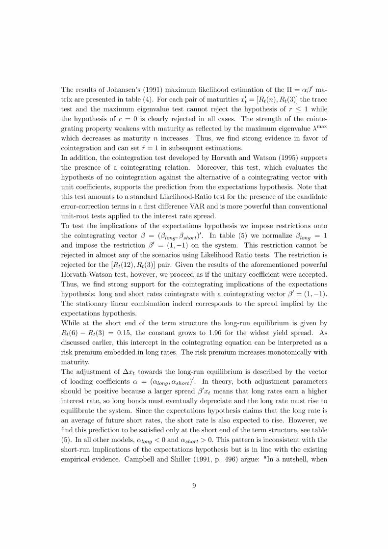
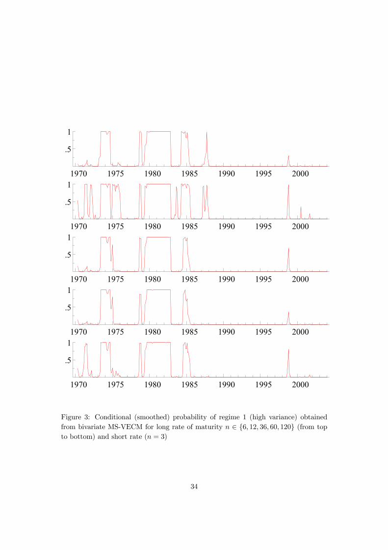
structure.14 This is consistent with the finding of a time-varying term premium on longrates, see Engle Lilien, and Robins (1987), that has been proposed as an explanationfor the failure of the expectations hypothesis to forecast interest rates. Furthermore,this lends support to the argument of Kozicki and Tinsley (2002) that more aggressivepolicy accompanied by a more volatile policy-controlled rate induces an upward shiftin the term premium.Fifth, regime 1 exhibits a mostly positive short-term drift while the drift in regime 2is negative. Not surprisingly, the adjustment of interest rates is much stronger duringperiods of high volatility.Sixth, the most remarkable regime shift occurs between 1979 and 1982, when the Fed-eral Reserve changed its operating procedures. In this sense the results mirror the find-ings of other papers reviewed above. Figure (3) presents the conditional (smoothed)probabilities of regime 1 for each interest rate pair. During the 1979-82 period regime1 prevails featuring high volatility. Regime 1 also reflects other phases of rising infla-tion expectations. Many of the dates of shifts to regime 1 correspond to the narrativeaccount of Goodfriend (1993, 1998). He identifies periods of "inflation scare" accom-panied by sharply rising long rates and decreasing anti-inflation credibility. However,the virtue of the regime-switching method is the ability to let the model detect regimeshifts endogenously. According to the Fisher equation, I(1) yields on long term bondsreflect long-run inflation expectations given a stationary real interest rate. Thus, shiftsin risk premia correspond to shifts in inflation expectations. Between 1979 and 1982risk premia at the short end rise while those at the long end fall. This indicatesthat long run inflation expectations decrease due to aggressive counter-inflation policyexpressed in sharply rising short rates while inflation expectations rise over the shorthorizon. Following periods of persistent inflation expectations during the early and thelate 1970s, the Fed under chairman Volcker engaged in aggressive disinflation policy.However, according to Goodfriend (1998), inflation expectations rose again in 1984.This re-emergence of inflation scare is reflected in the shift towards regime 1. Theregime shifts occurring in 1973/74 and 1984 are also found, among others, by Angand Bekaert (2002).15 In regime 2, the volatility of both interest rates is low. There-fore, state 2 reflects monetary stability. Regime 2 coincides with the chairmanship ofAlan Greenspan since 1987, indicating persistent anti-inflation credibility and a stablemonetary environment.Seventh, to facilitate the interpretation of the resulting regime-dependent adjustmentcoefficients and drift terms, we look at the common trends-implication of the coin-

14Cogley (2003) also finds that the risk premium on long-term bonds is connected to the varianceof the short rate. He interprets this result as evidence of the connection between uncertainty aboutthe target of monetary policy and mean yield spreads.15The shift to regime 1 in 1973 might also reflect tensions in U.S. bond markets during the final

breakup of the Bretton Woods system of fixed exchange rates.

15

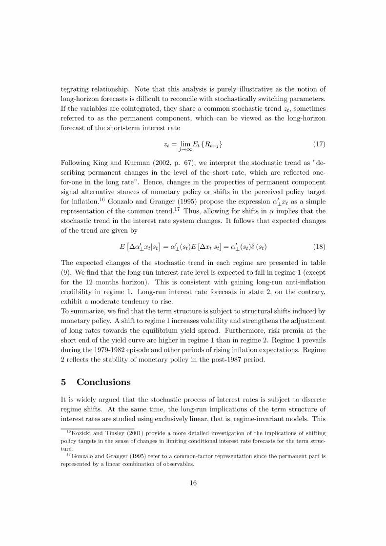
tegrating relationship. Note that this analysis is purely illustrative as the notion oflong-horizon forecasts is difficult to reconcile with stochastically switching parameters.If the variables are cointegrated, they share a common stochastic trend zt, sometimesreferred to as the permanent component, which can be viewed as the long-horizonforecast of the short-term interest rate

zt = limj→∞

Et {Rt+j} (17)

Following King and Kurman (2002, p. 67), we interpret the stochastic trend as "de-scribing permanent changes in the level of the short rate, which are reflected one-for-one in the long rate". Hence, changes in the properties of permanent componentsignal alternative stances of monetary policy or shifts in the perceived policy targetfor inflation.16 Gonzalo and Granger (1995) propose the expression α0⊥xt as a simplerepresentation of the common trend.17 Thus, allowing for shifts in α implies that thestochastic trend in the interest rate system changes. It follows that expected changesof the trend are given by

E£∆α0⊥xt|st

¤= α0⊥(st)E [∆xt|st] = α0⊥(st)δ (st) (18)

The expected changes of the stochastic trend in each regime are presented in table(9). We find that the long-run interest rate level is expected to fall in regime 1 (exceptfor the 12 months horizon). This is consistent with gaining long-run anti-inflationcredibility in regime 1. Long-run interest rate forecasts in state 2, on the contrary,exhibit a moderate tendency to rise.To summarize, we find that the term structure is subject to structural shifts induced bymonetary policy. A shift to regime 1 increases volatility and strengthens the adjustmentof long rates towards the equilibrium yield spread. Furthermore, risk premia at theshort end of the yield curve are higher in regime 1 than in regime 2. Regime 1 prevailsduring the 1979-1982 episode and other periods of rising inflation expectations. Regime2 reflects the stability of monetary policy in the post-1987 period.

5 Conclusions

It is widely argued that the stochastic process of interest rates is subject to discreteregime shifts. At the same time, the long-run implications of the term structure ofinterest rates are studied using exclusively linear, that is, regime-invariant models. This

16Kozicki and Tinsley (2001) provide a more detailed investigation of the implications of shiftingpolicy targets in the sense of changes in limiting conditional interest rate forecasts for the term struc-ture.17Gonzalo and Granger (1995) refer to a common-factor representation since the permanent part is

represented by a linear combination of observables.

16

paper argues that we can gain additional insights about the behavior of interest ratesand the shifts in monetary policy by studying these two issues jointly. In particular,the regime-switching dynamics of stationary term premia can only be studied in ageneralization of the cointegrated VAR model that allows for regime shifts.We employed a Markov-switching VECM approach to analyze the behavior of theU.S. term structure given that interest rates of different maturity share a commonstochastic trend. While the long-run equilibrium relation implied by the expectationshypothesis is likely to be stable over time, the short-run adjustment of interest ratestowards the equilibrium as well as the term premium embedded in long rates shiftbetween unobservable regimes governed by a first order Markov chain.In accordance to the literature, we found these regime shifts to closely mirror thestance and the strategy of monetary policy. During the 1979-82 shift of the FederalReserve from interest rate targeting to money growth targeting and other phases ofinflation scare a regime prevails that exhibits a much higher variance and a muchfaster equilibrium adjustment than in the alternative regime. The risk premium atthe short end increases while risk premia on long bonds decrease in this regime. Thismeans that monetary policy leads to rising short-run inflation expectations but fallinglong-run inflation expectations. A regime with remarkable stability in terms of riskpremia and interest rate volatility prevails in the post-1987 period. Thus, this papercontributed to closing the gap between two rather separate strands of the literatureand, at the same time, provided evidence on the information content of the termstructure over time.

17

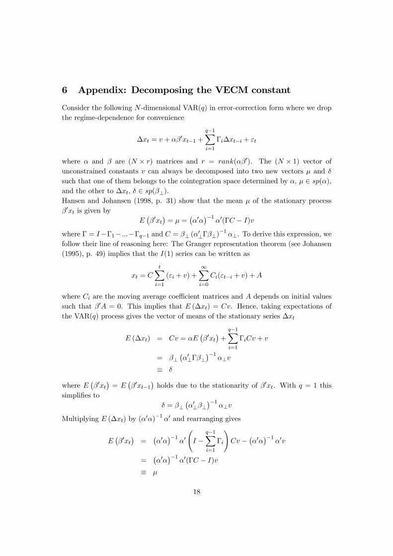
6 Appendix: Decomposing the VECM constant

Consider the following N -dimensional VAR(q) in error-correction form where we dropthe regime-dependence for convenience

∆xt = v + αβ0xt−1 +q−1Xi=1

Γi∆xt−i + εt

where α and β are (N × r) matrices and r = rank(αβ0). The (N × 1) vector ofunconstrained constants v can always be decomposed into two new vectors µ and δ

such that one of them belongs to the cointegration space determined by α, µ ∈ sp(α),and the other to ∆xt, δ ∈ sp(β⊥).Hansen and Johansen (1998, p. 31) show that the mean µ of the stationary processβ0xt is given by

E¡β0xt

¢= µ =

¡α0α

¢−1α0(ΓC − I)v

where Γ = I−Γ1− ...−Γq−1 and C = β⊥ (α0⊥Γβ⊥)−1 α⊥. To derive this expression, we

follow their line of reasoning here: The Granger representation theorem (see Johansen(1995), p. 49) implies that the I(1) series can be written as

xt = CtXi=1

(εi + v) +∞Xi=0

Ci(εt−i + v) +A

where Ci are the moving average coefficient matrices and A depends on initial valuessuch that β0A = 0. This implies that E (∆xt) = Cv. Hence, taking expectations ofthe VAR(q) process gives the vector of means of the stationary series ∆xt

E (∆xt) = Cv = αE¡β0xt

¢+

q−1Xi=1

ΓiCv + v

= β⊥¡α0⊥Γβ⊥

¢−1α⊥v

≡ δ

where E¡β0xt

¢= E

¡β0xt−1

¢holds due to the stationarity of β0xt. With q = 1 this

simplifies toδ = β⊥

¡α0⊥β⊥

¢−1α⊥v

Multiplying E (∆xt) by (α0α)−1 α0 and rearranging gives

E¡β0xt

¢=

¡α0α

¢−1α0ÃI −

q−1Xi=1

Γi

!Cv − ¡α0α¢−1 α0v

=¡α0α

¢−1α0(ΓC − I)v

≡ µ

18

If q = 1, this reduces to

E¡β0xt

¢=

¡α0α

¢−1α0(ΓC − I)v

=¡α0α

¢−1α0hβ⊥¡α0⊥Γβ⊥

¢−1α⊥ − I

iv

=¡α0α

¢−1α0h−α ¡β0α¢−1 β0i v

= − ¡β0α¢−1 β0vNote that the vectors of equilibrium means and of drift terms are related by

v = Γδ − αµ

Let us now re-introduce regime-dependent coefficients α (st) , v (st), and Γi (st) as de-scribed in the text. The MS-VECM enables us to decompose the regime-dependentconstant v (st) into regime-specific attractor sets (µ (st) , δ (st)) as explained in the text.This means there are (N−r) linearly independent but state-dependent drifts collectedin δ and r linearly independent but state-dependent equilibrium means collected in µ

E (∆xt|st) = δ (st)

E¡β0xt−1|st

¢= µ (st)

Hence, both ∆xt and β0xt−1 are expressed as deviations from their regime-specificmeans.

19

References

[1] Aït-Sahalia, Y. (1996): "Testing Continous-Time Models of the Spot InterestRate", The Review of Financial Studies 9, 385-426.

[2] Andrews, D. W. K. and W. Ploberger (1994): ”Optimal tests when a nuisanceparameter is present only under the alternative”, Econometrica 62, 1383-1414.

[3] Ang, A. and G. Bekaert (2002): "Regime Switches in Interest Rates", Journal ofBusiness and Economic Statistics 20, 163-182.

[4] Bansal, R., G. Tauchen, and H. Zhou (2003): "Regime-Shifts, Risk Premiums inthe Term Structure, and the Business Cycle", unpublished, Duke University.

[5] Bekaert, G., R. J. Hodrick, and D. A. Marshall (2001): "Peso problem explana-tions for term structure anomalies", Journal of Monetary Economics 48, 241-270.

[6] Brock, W. A., W. D. Dechert, J. A. Scheinkman, and B. LeBaron (1996): "A testfor independence based on the correlation dimension", Econometric Reviews 15,197-235.

[7] Campbell, J. Y. and R. J. Shiller (1987): "Cointegration and Tests of PresentValue Models", Journal of Political Economy 95, 1062-1088.

[8] Campbell, J. Y. and R. J. Shiller (1991): "Yield Spreads and Interest Rate Move-ments: A Bird’s Eye View", Review of Economic Studies 58, 495-514.

[9] Clarida, R. H., L. Sarno, M. P. Taylor, and G. Valente (2003): "The out-of-samplesuccess of term structure models as exchange rate predictors: a step beyond",Journal of International Economics 60, 61-83.

[10] Cogley, T. (2003): "An Exploration of Evolving Term Structure Relations", un-published, University of California, Davis.

[11] Cuthbertson, K. (1996): "The Expectations Hypothesis of the Term Structure:The UK Interbank Market", The Economic Journal 106, 578-592.

[12] Dai, Q., K. J. Singleton, and W. Yang (2003): "Regime Shifts in a DynamicTerm Structure Model of U.S. Treasury Bond Yields", unpublished, Stern Schoolof Business.

[13] Engle, R. F., D. M. Lilien, and R. P. Robins (1987): Estimating Time VaryingRisk Premia in the Term Structure: The ARCH-M Model", Econometrica 55,391-407.

20

[14] Engsted, T. and K. Nyholm (2000): "Regime shifts in the Danish term structureof interest rates", Empirical Economics 25, 1-13.

[15] Engsted, T. and C. Tanggaard (1994): "Cointegration and the US Term Struc-ture", Journal of Banking and Finance 18, 167-181.

[16] Francis, N. and M. T. Owyang (2003): "Monetary Policy in a Markov-SwitchingVECM: Implications for the Cost of Disinflation and the Price Puzzle", unpub-lished, Federal Reserve Bank of St. Louis.

[17] Fuhrer, J. C. (1996): "Monetary Policy Shifts and Long-Term Interest Rates",Quarterly Journal of Economics 111, 1183-1209.

[18] Garcia, R. (1998): ”Asymptotic Null Distribution of the Likelihood Ratio Test inMarkov Switching Models”, International Economic Review 39, 763-788.

[19] Gonzalo, J. and C. Granger (1995): "Estimation of Common Long-Memory Com-ponents in Cointegrated Systems", Journal of Business and Economic Statistics13, 27-35.

[20] Goodfriend, M. (1993): "Interest Rate Policy and the Inflation Scare Problem:1979-1992", Economic Quarterly 79, Federal Reserve Bank of Richmond, 1-23.

[21] Goodfriend, M. (1998): "Using the Term Structure of Interest Rates for MonetaryPolicy", Economic Quarterly 84, Federal Reserve Bank of Richmond, 13-30.

[22] Gray, S. F. (1996): "Modeling the conditional distribution of interest rates as aregime-switching process", Journal of Financial Economics 42, 27-62.

[23] Gregory, A. W. and B. E. Hansen (1996): "Residual-based tests for cointegrationin models with regime shifts", Journal of Econometrics 70, 99-126.

[24] Gutiérrez, M.-J. and J. Vázquez (2003): "The changing behavior of the termstructure of post-war U.S. interest rates", unpublished, Universidad del País Vasco.

[25] Hall, A., D., H. M. Anderson, and C. W. J. Granger (1992): "A CointegrationAnalysis of Treasury Bill Yields", The Review of Economics and Statistics 74,116-126.

[26] Hamilton, J. D. (1988): ”Rational-Expectations Econometric Analysis of Changesin Regime: An Investigation of the Term Structure of Interest Rates”, Journal ofEconomic Dynamics and Control 12, 385-423.

[27] Hansen, B. E. (1992a): "Tests for Parameter Instability in Regressions with I(1)Processes", Journal of Business and Economic Statistics 10, 321-335.

21

[28] Hansen, B. E. (1992b): ”The Likelihood Ratio Test under Nonstandard Condi-tions: Testing the Markov Switching Model of GNP”, Journal of Applied Econo-metrics 7, S61-S82.

[29] Hansen, B. E. and B. Seo (2002): "Testing for two-regime threshold cointegrationin vector error-correction models", Journal of Econometrics 110, 293-318.

[30] Hansen, H. and S. Johansen (1998): Workbook on Cointegration, Oxford: OxfordUniversity Press.

[31] Hansen, H. and S. Johansen (1999): "Some tests for parameter constancy incointegrated VAR-models", Econometrics Journal 2, 306-333.

[32] Hansen, P. R. (2003): "Structural Changes in the Cointegrated Vector Autore-gressive Model", Journal of Econometrics 114, 261-295.

[33] Horvath, M. T. K. and M. W. Watson (1995): "Testing for cointegration whensome of the cointegrating vectors are prespecified", Econometric Theory 11, 984-1014.

[34] Johansen, S. (1991): "Estimation and Hypothesis Testing of Cointegration Vectorsin Gaussian Vector Autoregressive Models", Econometrica 59, 1551-1580.

[35] King, R. G. and A. Kurmann (2002): "Expectations and the Term Structureof Interest Rates: Evidence and Implications", Economic Quarterly 88, FederalReserve Bank of Richmond, 49-95.

[36] Kozicki, S. and P. A. Tinsley (2001): "Shifting endpoints in the term structure ofinterest rates", Journal of Monetary Economics 47, 613-652.

[37] Kozicki, S. and P. A. Tinsley (2002): "Term Premia: Endogenous Constraints onMonetary Policy", Working Paper, No. 02-07, Federal Reserve Bank of KansasCity.

[38] Krolzig, H.-M. (1997): "Statistical Analysis of Cointegrated VAR Processes withMarkovian Regime Shifts", unpublished, Nuffield College, Oxford.

[39] Krolzig, H.-M. (1998), ”Econometric Modeling of Markov-Switching Vector Au-toregressions using MSVAR for Ox”, unpublished, Nuffield College, Oxford.

[40] Krolzig, H.-M., M. Marcellino, and G. E. Mizon (2002): ”A Markov-switching vec-tor equilibrium correction model of the UK labour market”, Empirical Economics27, 233-254.

22

[41] Kugler, P. (1996): "The term structure of interest rates and regime shifts: Someempirical results", Economics Letters 50, 121-126.

[42] Osterwald-Lenum, M. (1992): "A Note with Quantiles of the Asymptotic Distri-bution of the Maximum Likelihood Cointegration Rank Test Statistics", OxfordBulletin of Economics and Statistics 54, 461-472.

[43] Psaradakis, Z. and N. Spagnolo (2002): "Power Properties of Nonlinearity Testsfor Time Series with Markov Regimes", Studies in Nonlinear Dynamics andEconometrics 6, article 2.

[44] Saikkonen, P. and R. Luukkonen (1997): "Testing cointegration in infinite ordervector autoregressive processes", Journal of Econometrics 81, 93-126.

[45] Sarno, L., D. L. Thornton, and G. Valente (2002): "Federal Funds Rate Predic-tion", Working Paper, No. 2002-005B, Federal Reserve Bank of St. Louis.

[46] Seo, B. (2003): "Nonlinear mean reversion in the term structure of interest rates",Journal of Economic Dynamics and Control 27, 2243-2265.

[47] Shea, G. S. (1992): "Benchmarking the Expectations Hypothesis of the Interest-Rate Term Structure: An Analysis of Cointegration Vectors", Journal of Businessand Economic Statistics 10, 347-366.

[48] Sola, M. and J. Driffill (1994): "Testing the term structure of interest rates usinga stationary vector autoregression with regime switching", Journal of EconomicDynamics and Control 18, 601-628.

23

Table 1: Descriptive statistics of interest rate spreads

spread (in %) mean max. min. std.dev. skew kurt # obs.Rt(6)−Rt(3) 0.135 1.450 -1.010 0.222 -0.069 10.812 410Rt(12)−Rt(3) 0.221 2.375 -1.991 0.455 -0.194 6.568 410Rt(36)−Rt(3) 1.145 4.110 -2.010 0.868 -0.454 3.881 410Rt(60)−Rt(3) 1.390 4.330 -2.250 1.072 -0.596 3.358 410Rt(120)−Rt(3) 1.647 4.420 -2.650 1.308 -0.604 2.995 410

Table 2: Unit-root testsseries specification ADF PP KPSS ADF(4) PP(4) KPSS(4)Rt(3) const. -1.17 -1.51 0.85∗∗∗ -1.75 -1.87 2.58∗∗∗

no const. -1.03 -1.29 -1.16 -1.27Rt(6) const. -1.49 -1.71 0.91∗∗∗ -1.58 -1.71 2.78∗∗∗

no const. -1.02 -1.22 -1.12 -1.21Rt(12) const. -1.07 -1.67 0.92∗∗∗ -1.46 -1.64 2.84∗∗∗

no const. -0.98 -1.18 -1.11 -1.16Rt(36) const. -1.26 -1.43 0.93∗∗∗ -1.28 -1.41 2.91∗∗∗

no const. -0.91 -1.02 -0.99 -1.04Rt(60) const. -1.21 -1.39 0.93∗∗∗ -1.25 -1.35 2.91∗∗∗

no const. -0.84 -0.96 -0.92 -0.96Rt(120) const. -1.13 -1.26 0.89∗∗∗ -1.20 -1.23 2.84∗∗∗

no const. -0.73 -0.82 -0.83 -0.82

Notes: Unit-root tests with and without intercept term. ADF denotes the test statisticfrom the augmented Dickey-Fuller test, PP denotes the test statistic from the Phillips-Perron test, and KPSS is the Kwiatkowski-Phillips-Schmidt-Shin test statistic. WhileADF and PP test the hypothesis of a unit-root, KPSS tests the Null of stationarityagainst the unit-root hypothesis. The lag order for the ADF test is chosen accordingto the Schwartz criterion; the PP and the KPSS test are specified using the Bartlettkernel with automatic Newey-West bandwidth selection. The last three columns reporttest results with a lag length set to four. A significance level of 1%, 5%, and 10% isindicated by ∗∗∗, ∗∗, and ∗.

24

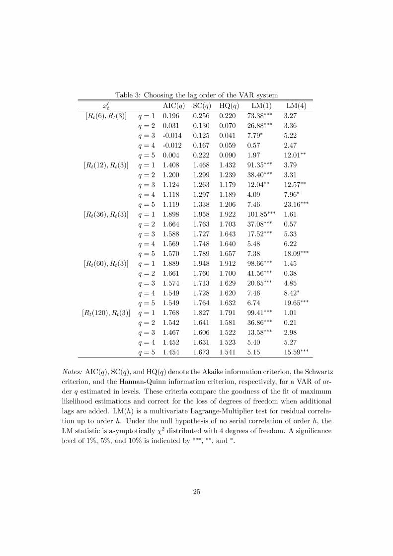
Table 3: Choosing the lag order of the VAR system

x0t AIC(q) SC(q) HQ(q) LM(1) LM(4)[Rt(6), Rt(3)] q = 1 0.196 0.256 0.220 73.38∗∗∗ 3.27

q = 2 0.031 0.130 0.070 26.88∗∗∗ 3.36q = 3 -0.014 0.125 0.041 7.79∗ 5.22q = 4 -0.012 0.167 0.059 0.57 2.47q = 5 0.004 0.222 0.090 1.97 12.01∗∗

[Rt(12), Rt(3)] q = 1 1.408 1.468 1.432 91.35∗∗∗ 3.79q = 2 1.200 1.299 1.239 38.40∗∗∗ 3.31q = 3 1.124 1.263 1.179 12.04∗∗ 12.57∗∗

q = 4 1.118 1.297 1.189 4.09 7.96∗

q = 5 1.119 1.338 1.206 7.46 23.16∗∗∗

[Rt(36), Rt(3)] q = 1 1.898 1.958 1.922 101.85∗∗∗ 1.61q = 2 1.664 1.763 1.703 37.08∗∗∗ 0.57q = 3 1.588 1.727 1.643 17.52∗∗∗ 5.33q = 4 1.569 1.748 1.640 5.48 6.22q = 5 1.570 1.789 1.657 7.38 18.09∗∗∗

[Rt(60), Rt(3)] q = 1 1.889 1.948 1.912 98.66∗∗∗ 1.45q = 2 1.661 1.760 1.700 41.56∗∗∗ 0.38q = 3 1.574 1.713 1.629 20.65∗∗∗ 4.85q = 4 1.549 1.728 1.620 7.46 8.42∗

q = 5 1.549 1.764 1.632 6.74 19.65∗∗∗

[Rt(120), Rt(3)] q = 1 1.768 1.827 1.791 99.41∗∗∗ 1.01q = 2 1.542 1.641 1.581 36.86∗∗∗ 0.21q = 3 1.467 1.606 1.522 13.58∗∗∗ 2.98q = 4 1.452 1.631 1.523 5.40 5.27q = 5 1.454 1.673 1.541 5.15 15.59∗∗∗

Notes: AIC(q), SC(q), and HQ(q) denote the Akaike information criterion, the Schwartzcriterion, and the Hannan-Quinn information criterion, respectively, for a VAR of or-der q estimated in levels. These criteria compare the goodness of the fit of maximumlikelihood estimations and correct for the loss of degrees of freedom when additionallags are added. LM(h) is a multivariate Lagrange-Multiplier test for residual correla-tion up to order h. Under the null hypothesis of no serial correlation of order h, theLM statistic is asymptotically χ2 distributed with 4 degrees of freedom. A significancelevel of 1%, 5%, and 10% is indicated by ∗∗∗, ∗∗, and ∗.

25

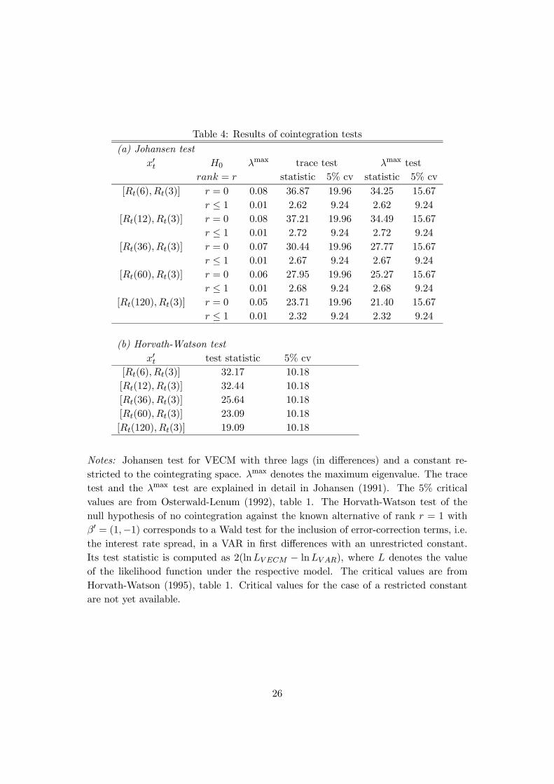
Table 4: Results of cointegration tests

(a) Johansen testx0t H0 λmax trace test λmax test

rank = r statistic 5% cv statistic 5% cv[Rt(6), Rt(3)] r = 0 0.08 36.87 19.96 34.25 15.67

r ≤ 1 0.01 2.62 9.24 2.62 9.24[Rt(12), Rt(3)] r = 0 0.08 37.21 19.96 34.49 15.67

r ≤ 1 0.01 2.72 9.24 2.72 9.24[Rt(36), Rt(3)] r = 0 0.07 30.44 19.96 27.77 15.67

r ≤ 1 0.01 2.67 9.24 2.67 9.24[Rt(60), Rt(3)] r = 0 0.06 27.95 19.96 25.27 15.67

r ≤ 1 0.01 2.68 9.24 2.68 9.24[Rt(120), Rt(3)] r = 0 0.05 23.71 19.96 21.40 15.67

r ≤ 1 0.01 2.32 9.24 2.32 9.24

(b) Horvath-Watson testx0t test statistic 5% cv

[Rt(6), Rt(3)] 32.17 10.18[Rt(12), Rt(3)] 32.44 10.18[Rt(36), Rt(3)] 25.64 10.18[Rt(60), Rt(3)] 23.09 10.18[Rt(120), Rt(3)] 19.09 10.18

Notes: Johansen test for VECM with three lags (in differences) and a constant re-stricted to the cointegrating space. λmax denotes the maximum eigenvalue. The tracetest and the λmax test are explained in detail in Johansen (1991). The 5% criticalvalues are from Osterwald-Lenum (1992), table 1. The Horvath-Watson test of thenull hypothesis of no cointegration against the known alternative of rank r = 1 withβ0 = (1,−1) corresponds to a Wald test for the inclusion of error-correction terms, i.e.the interest rate spread, in a VAR in first differences with an unrestricted constant.Its test statistic is computed as 2(lnLV ECM − lnLV AR), where L denotes the valueof the likelihood function under the respective model. The critical values are fromHorvath-Watson (1995), table 1. Critical values for the case of a restricted constantare not yet available.

26

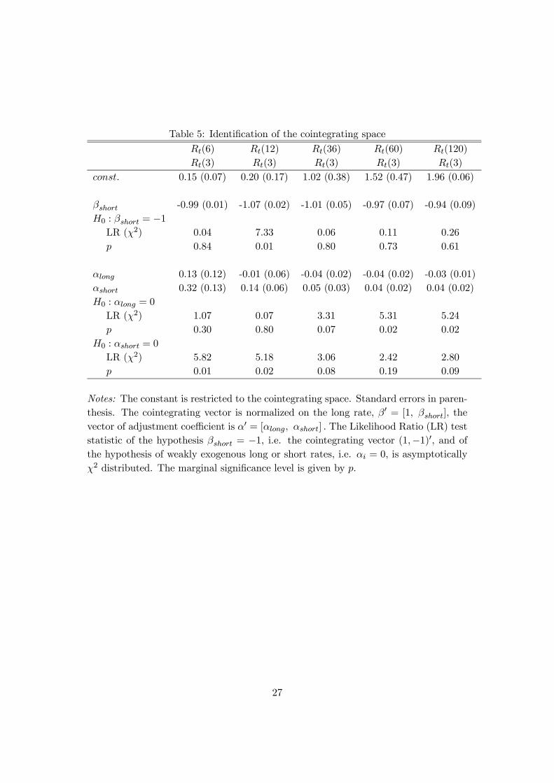
Table 5: Identification of the cointegrating space

Rt(6)

Rt(3)

Rt(12)

Rt(3)

Rt(36)

Rt(3)

Rt(60)

Rt(3)

Rt(120)

Rt(3)

const. 0.15 (0.07) 0.20 (0.17) 1.02 (0.38) 1.52 (0.47) 1.96 (0.06)

βshort -0.99 (0.01) -1.07 (0.02) -1.01 (0.05) -0.97 (0.07) -0.94 (0.09)H0 : βshort = −1LR (χ2) 0.04 7.33 0.06 0.11 0.26p 0.84 0.01 0.80 0.73 0.61

αlong 0.13 (0.12) -0.01 (0.06) -0.04 (0.02) -0.04 (0.02) -0.03 (0.01)αshort 0.32 (0.13) 0.14 (0.06) 0.05 (0.03) 0.04 (0.02) 0.04 (0.02)H0 : αlong = 0

LR (χ2) 1.07 0.07 3.31 5.31 5.24p 0.30 0.80 0.07 0.02 0.02

H0 : αshort = 0

LR (χ2) 5.82 5.18 3.06 2.42 2.80p 0.01 0.02 0.08 0.19 0.09

Notes: The constant is restricted to the cointegrating space. Standard errors in paren-thesis. The cointegrating vector is normalized on the long rate, β0 = [1, βshort], thevector of adjustment coefficient is α0 = [αlong, αshort] . The Likelihood Ratio (LR) teststatistic of the hypothesis βshort = −1, i.e. the cointegrating vector (1,−1)0, and ofthe hypothesis of weakly exogenous long or short rates, i.e. αi = 0, is asymptoticallyχ2 distributed. The marginal significance level is given by p.

27

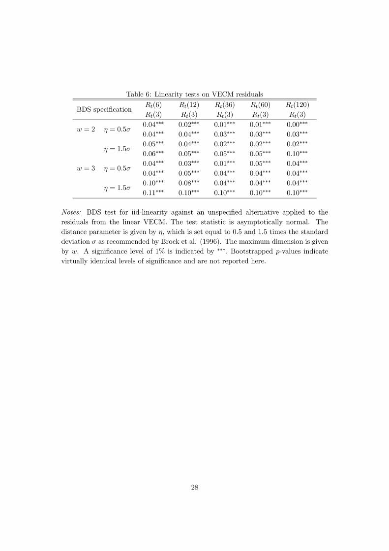
Table 6: Linearity tests on VECM residuals

BDS specificationRt(6)

Rt(3)

Rt(12)

Rt(3)

Rt(36)

Rt(3)

Rt(60)

Rt(3)

Rt(120)

Rt(3)

w = 2 η = 0.5σ0.04∗∗∗

0.04∗∗∗0.02∗∗∗

0.04∗∗∗0.01∗∗∗

0.03∗∗∗0.01∗∗∗

0.03∗∗∗0.00∗∗∗

0.03∗∗∗

η = 1.5σ0.05∗∗∗

0.06∗∗∗0.04∗∗∗

0.05∗∗∗0.02∗∗∗

0.05∗∗∗0.02∗∗∗

0.05∗∗∗0.02∗∗∗

0.10∗∗∗

w = 3 η = 0.5σ0.04∗∗∗

0.04∗∗∗0.03∗∗∗

0.05∗∗∗0.01∗∗∗

0.04∗∗∗0.05∗∗∗

0.04∗∗∗0.04∗∗∗

0.04∗∗∗

η = 1.5σ0.10∗∗∗

0.11∗∗∗0.08∗∗∗

0.10∗∗∗0.04∗∗∗

0.10∗∗∗0.04∗∗∗

0.10∗∗∗0.04∗∗∗

0.10∗∗∗

Notes: BDS test for iid-linearity against an unspecified alternative applied to theresiduals from the linear VECM. The test statistic is asymptotically normal. Thedistance parameter is given by η, which is set equal to 0.5 and 1.5 times the standarddeviation σ as recommended by Brock et al. (1996). The maximum dimension is givenby w. A significance level of 1% is indicated by ∗∗∗. Bootstrapped p-values indicatevirtually identical levels of significance and are not reported here.

28

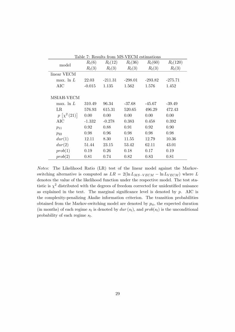
Table 7: Results from MS-VECM estimations

modelRt(6)

Rt(3)

Rt(12)

Rt(3)

Rt(36)

Rt(3)

Rt(60)

Rt(3)

Rt(120)

Rt(3)

linear VECMmax. ln L 22.03 -211.31 -298.01 -293.82 -275.71AIC -0.015 1.135 1.562 1.576 1.452

MSIAH-VECMmax. ln L 310.49 96.34 -37.68 -45.67 -39.49LR 576.93 615.31 520.65 496.29 472.43p£χ2 (21)

¤0.00 0.00 0.00 0.00 0.00

AIC -1.332 -0.278 0.383 0.458 0.392p11 0.92 0.88 0.91 0.92 0.90p22 0.98 0.96 0.98 0.98 0.98dur(1) 12.11 8.30 11.55 12.79 10.36dur(2) 51.44 23.15 53.42 62.11 43.01prob(1) 0.19 0.26 0.18 0.17 0.19prob(2) 0.81 0.74 0.82 0.83 0.81

Notes: The Likelihood Ratio (LR) test of the linear model against the Markov-switching alternative is computed as LR = 2(lnLMS−V ECM − lnLV ECM) where Ldenotes the value of the likelihood function under the respective model. The test sta-tistic is χ2 distributed with the degrees of freedom corrected for unidentified nuisanceas explained in the text. The marginal significance level is denoted by p. AIC isthe complexity-penalizing Akaike information criterion. The transition probabilitiesobtained from the Markov-switching model are denoted by pii, the expected duration(in months) of each regime st is denoted by dur (st), and prob(st) is the unconditionalprobability of each regime st.

29

Table 8: Parameter estimates from the MSIAH-VECMRt(6)

Rt(3)

Rt(12)

Rt(3)

Rt(36)

Rt(3)

Rt(60)

Rt(3)

Rt(120)

Rt(3)

v (1)0.027 (0.10)

−0.014 (0.11)0.206 (0.13)

0.001 (0.14)

0.101 (0.09)

−0.020 (0.13)0.097 (0.07)

−0.028 (0.13)0.089 (0.06)

−0.034 (0.12)

v (2)−0.023 (0.02)−0.039 (0.02)

−0.030 (0.03)−0.080 (0.02)

0.003 (0.04)

−0.066 (0.03)0.012 (0.03)

−0.055 (0.02)0.004 (0.03)

−0.062 (0.02)

α(1)0.120 (0.34)

0.351 (0.38)

−0.236 (0.14)−0.030 (0.15)

−0.141 (0.07)0.036 (0.10)

−0.134 (0.05)0.052 (0.10)

−0.103 (0.04)0.065 (0.08)

α(2)0.099 (0.10)

0.239 (0.09)

0.032 (0.05)

0.135 (0.04)

−0.010 (0.03)0.049 (0.02)

−0.014 (0.02)0.033 (0.01)

−0.007 (0.01)0.030 (0.01)

Σ̃ (1)0.874

0.960

0.760

0.836

0.640

0.959

0.543

0.975

0.453

0.942

Σ̃ (2)0.232

0.211

0.233

0.170

0.276

0.208

0.259

0.213

0.232

0.198

Notes: Parameter estimates of bivariate MS-VECM. The regime-dependent vectorv (st) contains the intercept terms, the regime-dependent error-correction coefficientsare given by α (st), and the diagonal elements (the variances) of the regime-dependentvariance-covariance matrices are given by Σ̃ (st). Asymptotic standard errors in paren-thesis.

30

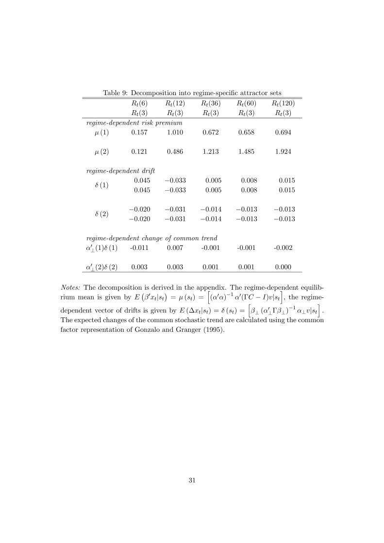
Table 9: Decomposition into regime-specific attractor sets

Rt(6)

Rt(3)

Rt(12)

Rt(3)

Rt(36)

Rt(3)

Rt(60)

Rt(3)

Rt(120)

Rt(3)

regime-dependent risk premiumµ (1) 0.157 1.010 0.672 0.658 0.694

µ (2) 0.121 0.486 1.213 1.485 1.924

regime-dependent drift

δ (1)0.045

0.045

−0.033−0.033

0.005

0.005

0.008

0.008

0.015

0.015

δ (2)−0.020−0.020

−0.031−0.031

−0.014−0.014

−0.013−0.013

−0.013−0.013

regime-dependent change of common trendα0⊥(1)δ (1) -0.011 0.007 -0.001 -0.001 -0.002

α0⊥(2)δ (2) 0.003 0.003 0.001 0.001 0.000

Notes: The decomposition is derived in the appendix. The regime-dependent equilib-rium mean is given by E

¡β0xt|st

¢= µ (st) =

h(α0α)−1 α0(ΓC − I)v|st

i, the regime-

dependent vector of drifts is given by E (∆xt|st) = δ (st) =hβ⊥ (α0⊥Γβ⊥)

−1 α⊥v|sti.

The expected changes of the common stochastic trend are calculated using the commonfactor representation of Gonzalo and Granger (1995).

31

0

4

8

1 2

1 6

2 0

1 9 7 0 1 9 7 5 1 9 8 0 1 9 8 5 1 9 9 0 1 9 9 5 2 0 0 0

n = 6 n = 3

0

4

8

1 2

1 6

2 0

1 9 7 0 1 9 7 5 1 9 8 0 1 9 8 5 1 9 9 0 1 9 9 5 2 0 0 0

n = 1 2 n = 3

0

4

8

1 2

1 6

2 0

1 9 7 0 1 9 7 5 1 9 8 0 1 9 8 5 1 9 9 0 1 9 9 5 2 0 0 0

n = 3 6 n = 3

0

4

8

1 2

1 6

2 0

1 9 7 0 1 9 7 5 1 9 8 0 1 9 8 5 1 9 9 0 1 9 9 5 2 0 0 0

n = 6 0 n = 3

0

4

8

1 2

1 6

2 0

1 9 7 0 1 9 7 5 1 9 8 0 1 9 8 5 1 9 9 0 1 9 9 5 2 0 0 0

n = 1 2 0 n = 3

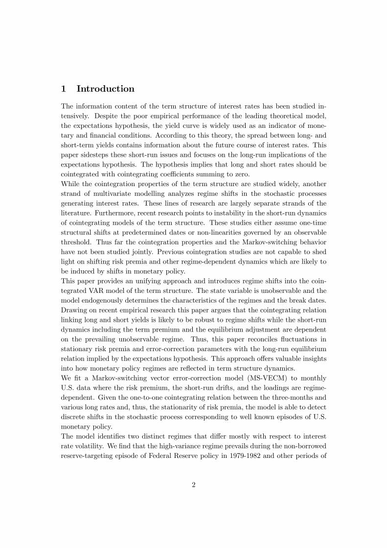
Figure 1: Interest rates (in % p.a.) on U.S. bonds of maturity n (in months), source:Federal Reserve Bank of St. Louis

32

-1 .5

-1 .0

-0 .5

0 .0

0 .5

1 .0

1 .5

1 9 70 1975 1980 1 985 19 90 199 5 2000

n= 6

-1

0

1

2

3

1970 1 975 19 80 198 5 1990 1995 2000

n= 12

-3

-2

-1

0

1

2

3

4

5

1970 1975 1980 1 985 19 90 199 5 2000

n= 3 6

-3

-2

-1

0

1

2

3

4

5

1970 1 975 19 80 198 5 1990 1995 2000

n = 60

-3

-2

-1

0

1

2

3

4

5

1970 1975 1980 1 985 19 90 199 5 2000

n= 120

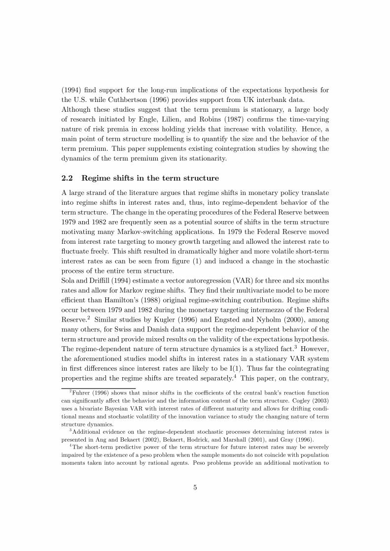
Figure 2: Spread (in percentage points) between annual interest rate on bond of ma-turity n (in months), Rt(n), and three-months bond, Rt(3)

33

1970 1975 1980 1985 1990 1995 2000

.5

1

1970 1975 1980 1985 1990 1995 2000

.5

1

1970 1975 1980 1985 1990 1995 2000

.5

1

1970 1975 1980 1985 1990 1995 2000

.5

1

1970 1975 1980 1985 1990 1995 2000

.5

1

Figure 3: Conditional (smoothed) probability of regime 1 (high variance) obtainedfrom bivariate MS-VECM for long rate of maturity n ∈ {6, 12, 36, 60, 120} (from topto bottom) and short rate (n = 3)

34