Embed Size (px)
Citation preview
Coho Reachability Analysis Tool Manual
Chao Yan
December 5, 2014 (Version 1.0)

2
Contents
1 Introduction 51.1 Installation . . . . . . . . . . . . . . . . . . . . . . . . . . . . . . 51.2 Simple Usage . . . . . . . . . . . . . . . . . . . . . . . . . . . . . 61.3 Examples . . . . . . . . . . . . . . . . . . . . . . . . . . . . . . . 61.4 Organization . . . . . . . . . . . . . . . . . . . . . . . . . . . . . 61.5 Learn More . . . . . . . . . . . . . . . . . . . . . . . . . . . . . . 6
2 Projectagon 92.1 Introduction . . . . . . . . . . . . . . . . . . . . . . . . . . . . . . 92.2 Projectagon structure and operations . . . . . . . . . . . . . . . . 102.3 Reachability algorithm and configuration . . . . . . . . . . . . . 122.4 Functions . . . . . . . . . . . . . . . . . . . . . . . . . . . . . . . 14
2.4.1 Projectagon . . . . . . . . . . . . . . . . . . . . . . . . . . 142.4.2 Reachability computation . . . . . . . . . . . . . . . . . . 14
3 Hybrid Automata 173.1 A Quick Start . . . . . . . . . . . . . . . . . . . . . . . . . . . . . 17
3.1.1 Problem . . . . . . . . . . . . . . . . . . . . . . . . . . . . 173.1.2 System dynamics . . . . . . . . . . . . . . . . . . . . . . . 173.1.3 Build hybrid automata . . . . . . . . . . . . . . . . . . . . 183.1.4 Perform computation . . . . . . . . . . . . . . . . . . . . 19
3.2 Hybrid Automata . . . . . . . . . . . . . . . . . . . . . . . . . . . 193.2.1 Automata states . . . . . . . . . . . . . . . . . . . . . . . 203.2.2 Automata transitions . . . . . . . . . . . . . . . . . . . . 213.2.3 Reachable computation algorithm . . . . . . . . . . . . . 21
3.3 Advanced Configuration . . . . . . . . . . . . . . . . . . . . . . . 223.3.1 Performance v.s Accuracy . . . . . . . . . . . . . . . . . . 223.3.2 Callbacks . . . . . . . . . . . . . . . . . . . . . . . . . . . 23
3.4 Functions . . . . . . . . . . . . . . . . . . . . . . . . . . . . . . . 23
4 Others 254.1 Linear Differential Inclusion . . . . . . . . . . . . . . . . . . . . . 254.2 Linear Programming . . . . . . . . . . . . . . . . . . . . . . . . . 254.3 Polygon Operations . . . . . . . . . . . . . . . . . . . . . . . . . 26
3

4 CONTENTS
4.4 Global Configurations . . . . . . . . . . . . . . . . . . . . . . . . 26
5 Examples 29
Chapter 1
Introduction
CRA (Coho Reachability Analysis tool) is a reachability analysis tool from theUniversity of British Columbia. It is based on the novel representation methodprojectagon[7, 3, 2]. It is originally developed for the Coho circuit verificationplatform. It is extended as a standalone tool for reachability analysis for AMSverification, hybrid systems, control systems, etc.
CRA provides two interfaces for users: the high-level hybrid automata inter-face and the detailed projectagon interface. The projectagon interface providesbasic projectagon operations which enable users to perform customized reach-ability computations. The hybrid automata interface accepts a user-providedhybrid system modeled by hybrid automata and computes all reachable systemstates automatically. It is recommended to use the hybrid automata interfacefor most users.
1.1 Installation
CRA is open-sourced. Users can download from github by:
git clone https :// github.com/dreamable/cra.git
CRA supports Linux, Unix and MacOS. It requires Matlab (R2008+) andJava (5.0+) installed in the system. It can be installed by:
cd cra
sh install.sh
Note that the installation script ask users a question that if the CPLEXlinearprogram solver available in the system or not. The CPLEX solver could improveperformance. To enable the solver, users must configure CPLEX and systemto support the CPLEXINT package1.
1http://control.ee.ethz.ch/ hybrid/cplexint.php
5
6 CHAPTER 1. INTRODUCTION
1.2 Simple Usage
CRA is a Matlab package. To use it, please first start Matlab, then run yourMatlab codes by:
cra_open
%user_code
cra_close
1.3 Examples
Examples are available under the example directory in the code. Please seechapter 5 for details.
1.4 Organization
chapter 2 presents the projectagon structure and operations. chapter 3 describethe hybrid automata interface. It is recommended to use the hybrid automatainterface for most users, while the projectagon interface are used for highlycustomized reachability computation. CRA also implemented some packageswhich could be useful for some users, e.g. linear program solver and polygonoperations based on arbitrary precision rational numbers. chapter 4 providesthe APIs of these functionalities. Examples that uses CRA are described inchapter 5.
1.5 Learn More
There are several paper published which are good sources to understand thehigher level ideas.
To understand implementation details, please use the Matlab help files by
help funcName
1.5. LEARN MORE 7
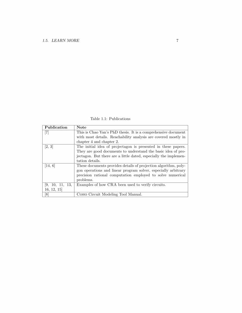
Table 1.1: Publications
Publication Note[7] This is Chao Yan’s PhD thesis. It is a comprehensive document
with most details. Reachability analysis are covered mostly inchapter 4 and chapter 2.
[2, 3] The initial idea of projectagon is presented in these papers.They are good documents to understand the basic idea of pro-jectagon. But there are a little dated, especially the implemen-tation details.
[14, 6] These documents provides details of projection algorithm, poly-gon operations and linear program solver, especially arbitraryprecision rational computation employed to solve numericalproblems.
[9, 10, 11, 13,16, 12, 15]
Examples of how CRA been used to verify circuits.
[8] Coho Circuit Modeling Tool Manual.

8 CHAPTER 1. INTRODUCTION
Chapter 2
Projectagon
2.1 Introduction
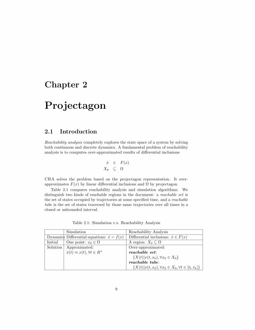
Reachability analysis completely explores the state space of a system by solvingboth continuous and discrete dynamics. A fundamental problem of reachabilityanalysis is to computes over-approximated results of differential inclusions
x ∈ F (x)
X0 ⊆ Ω
CRA solves the problem based on the projectagon representation. It over-approximates F (x) by linear differential inclusions and Ω by projectagon.
Table 2.1 compares reachability analysis and simulation algorithms. Wedistinguish two kinds of reachable regions in the document: a reachable set isthe set of states occupied by trajectories at some specified time, and a reachabletube is the set of states traversed by those same trajectories over all times in aclosed or unbounded interval.
Table 2.1: Simulation v.s. Reachability Analysis
Simulation Reachability AnalysisDynamics Differential equations: x = f(x) Differential inclusions: x ∈ F (x)Initial One point: x0 ∈ Ω A region: X0 ⊆ ΩSolution Approximated: Over-approximated:
x(t) ≈ x(t),∀t ∈ R+ reachable set :X(t)|x(t, x0),∀x0 ∈ X0
reachable tube :X(t)|x(t, x0),∀x0 ∈ X0,∀t ∈ [tl, th]
9
10 CHAPTER 2. PROJECTAGON
2.2 Projectagon structure and operations
projectagons are a data structure for representing high dimensional polyhedra bytheir projections onto two-dimensional planes, where these projection polygonsare not required to be convex. The representation is accurate and efficient: itcan represent non-convex polyhedra accurately, projectagon operations can beimplemented by efficient polygon operations. For more details, please see [7, 2].
The function ph create is to construct a projectagon.
ph = ph_create(dim ,planes ,hulls[,polys[,type ]]);
To create a projectagon, users need to provide
• dim: number of dimensions
• planes: projection planes, should be a dimx2 matrix
• polys: projection polygons, should be a cell, each item should be a polygonby poly create (see section 4.3).
• hulls: convex hull of projection polygons, should be a cell, each item shouldbe a convex polygon.
• type: projectagon types.
For example, to create a projectagon a unit cube,
polys 1 = poly_create ([0,0,1,1;0,1,1,0]);
polys 2 = poly_create ([0,0,1,1;0,1,1,0]);
polys 3 = poly_create ([0,0,1,1;0,1,1,0]);
ph = ph_create (3,[1,2;1,3;2,3],polys ,polys);
CRA supports three types of projectagon: 1) general (or non-convex) pro-jectagon, 2) convex projectagon, 3) bounding box. General projectagon is themost accurate representation with most complex operations; while boundingbox projectagon has most simple operations with largest error. This provideusers a way to get a trade-off between accuracy and performance for differentapplications. Usually, bounding box projectagon has so large approximationerror that can be rarely used for non-trivial problem. Convex projectagon ismore efficient for most simple problems with acceptable approximation error.General projectagon is used for complex problems that require small approx-imation error. Convex projectagon can be constructed from linear programs.Bounding box projectagon can be constructed from intervals. For example:
lp = lp_create ([1 ,0; -1 ,0;0 ,1;0 , -1] ,[1;0;1;0]);
ph = ph_createByLP(dim ,planes ,lp);
bbox = [0 ,1;0 ,1];
ph = ph_createByBox(dim ,planes ,bbox);
Different types of projectagons can be converted by
ph = ph_convert(ph ,new_type );
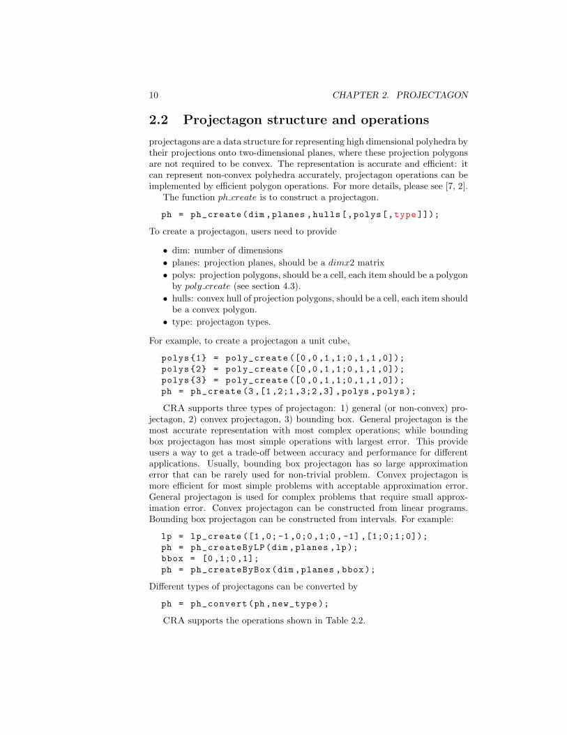
CRA supports the operations shown in Table 2.2.
2.2. PROJECTAGON STRUCTURE AND OPERATIONS 11
Table 2.2: Projectagon OperationsOperations Functions NoteUnion ph = ph union(set of ph) All ph must have same dim and
planesIntersect ph = ph intersect(set of ph) All ph must have same dim and
planesIntersect withline
ph = ph intersect(ph, line) Result is bloated to be a projec-tagon
Intersect withLP
ph = ph intersect(ph, lp)
Empty isempty = ph isempty(ph) check if the projectagon has fea-sible region or not
Simplify ph = ph simplify(ph) Simplify the projection poly-gons by over-approximate theregion slightly
Projection ph = ph project(ph,plane) Project the ph onto two-dimensional subspace.
Contain iscontain =ph contain(ph1,ph2)
Check if ph2 is contained by ph1
Contain Point iscontain=ph containPts(ph,pts)
Check if points are contained inthe ph or not
Canonical ph = ph canon(ph) make the projectagon canonicalMinkSum ph = ph minkSum(ph1,ph2) Only for bounding box projec-
tagonsChange planes ph = ph chplanes(ph,planes) Update ph to use a new set of
projection planes
12 CHAPTER 2. PROJECTAGON
2.3 Reachability algorithm and configuration
In CRA, reachable set and reachable tubes are computed by
new_ph = ph_advance(ph ,opt); % reachable set
ph_tube = ph_succ(ph ,new_ph ); % reachable tube
Reachable tubes for time interval [t0, t1] is over-approximated by bloating convexhull of reachable set for time t0 and t1.
ph[t0,t1] ∈ bloat(convex(pht0 , pht1));
User must define the system dynamics to compute reachable regions by
cra_cfg(set ,’modelFunc ’,modelFunc)
where modelFunc is a function handle of the format
models = modelFunc(lp)
The function accepts a CohoLP as input (see section 4.2 for details of CohoLP). The return of the function must be a structure with fields A, b, u, rep-resenting a linear differential inclusion model (LDI)1. A LDI mode is of theformat:
x ∈ Ax + b± u
To reduce linearization error, users can use the intersection of several lineardifferential inclusion models, by returning a cell of models.
The reachability algorithm accepts options which should be specified by astructure with the following fields:
• Parameters for computing models. A crucial step of reachability algo-rithm is to compute time step to be advance and corresponding maximummoving distance of all trajectories during the time interval. The choice oftimeStep,maxBloat pair affects both accuracy and performance signifi-cantly.
1see section 4.1 for details
2.3. REACHABILITY ALGORITHM AND CONFIGURATION 13
Fields Notemodel Three ways to compute the pair of timeStep,maxBloat.
– guess verify: Guess a pair of timeStep,maxBloat and verifythem at the end.
– bloatAmt: Compute timeStep from maxBloat.– timeStep: Use user provided maxStep with maxBloat.
Usually, the guess verify provides the best result for both ac-curacy and performance.
maxBloat Maximum moving distance of all trajectories in a single advancestep. It is used to compute timeStep for bloatAmt method.Users can specify different values for each variable and direction(increase or decrease)
maxStep Maximum time step.bloatAmt The fixed bloating amount. It is only for the bloatAmt method.timeStep The fixed user-provided time step. It is only for timeStep
method.prevBloatAmt,prevTimeStep
Interval usage for guess verify, should not be changed byusers.
ntries Maximum number of trying to guess a valid pair oftimeStep, bloatAmt for guess verify method.
• Parameters for finding projectagon faces to advance in each step.
Fields Noteobject Methods to compute object to advance. Valid value includes
– face-bloat: Advance projectagon faces individually. Faces arebloated outward for soundness.
– face-height: Advance projectagon faces individually. Theheight of faces are increased for soundness. Sometimes it hassmaller error than face-bloat.
– face-none: Advance projectagon face individually. Facesare not updated for soundness. It has smaller error thanface-bloat and face-height, but may not be sound. It re-quires non-zero error term in the linear differential inclusionmodel.
– face-all: Advance all faces and project them onto all slices.The result is sound, usually with large error bad slow perfor-mance.
– ph: Advance the whole projectagon. Only for convex orbounding-box projectagon.
maxEdgeLen Maximum length of polygon edges. When object is not ph,projection polygons are broken into short edges to reduce error.Larger value can reduce the number of faces but may increasemodel error.
useInterval Enable/disable the interval closure method to find more accu-rate faces for non-convex projectagon.
• Error control.
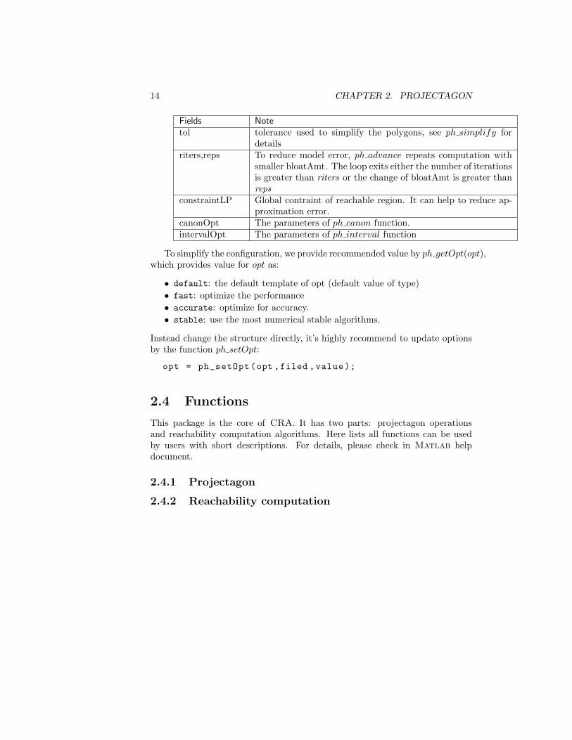
14 CHAPTER 2. PROJECTAGON
Fields Notetol tolerance used to simplify the polygons, see ph simplify for
detailsriters,reps To reduce model error, ph advance repeats computation with
smaller bloatAmt. The loop exits either the number of iterationsis greater than riters or the change of bloatAmt is greater thanreps
constraintLP Global contraint of reachable region. It can help to reduce ap-proximation error.
canonOpt The parameters of ph canon function.intervalOpt The parameters of ph interval function
To simplify the configuration, we provide recommended value by ph getOpt(opt),which provides value for opt as:
• default: the default template of opt (default value of type)
• fast: optimize the performance
• accurate: optimize for accuracy.
• stable: use the most numerical stable algorithms.
Instead change the structure directly, it’s highly recommend to update optionsby the function ph setOpt:
opt = ph_setOpt(opt ,filed ,value);
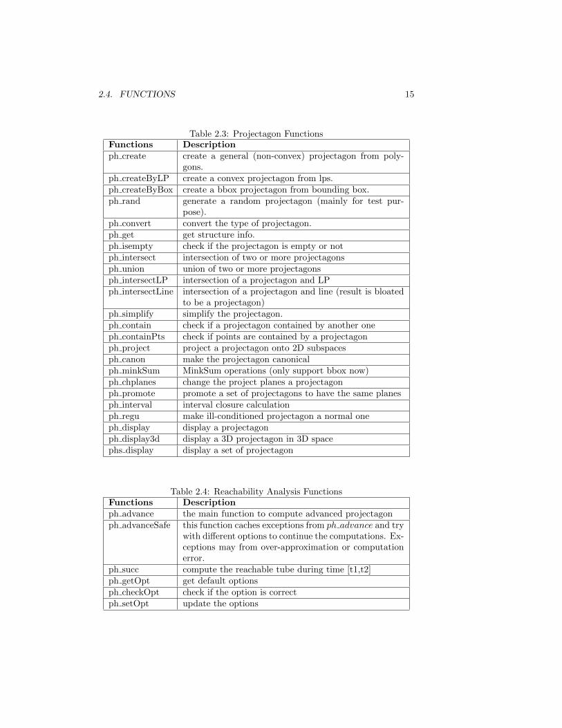
2.4 Functions
This package is the core of CRA. It has two parts: projectagon operationsand reachability computation algorithms. Here lists all functions can be usedby users with short descriptions. For details, please check in Matlab helpdocument.
2.4.1 Projectagon
2.4.2 Reachability computation
2.4. FUNCTIONS 15
Table 2.3: Projectagon FunctionsFunctions Descriptionph create create a general (non-convex) projectagon from poly-
gons.ph createByLP create a convex projectagon from lps.ph createByBox create a bbox projectagon from bounding box.ph rand generate a random projectagon (mainly for test pur-
pose).ph convert convert the type of projectagon.ph get get structure info.ph isempty check if the projectagon is empty or notph intersect intersection of two or more projectagonsph union union of two or more projectagonsph intersectLP intersection of a projectagon and LPph intersectLine intersection of a projectagon and line (result is bloated
to be a projectagon)ph simplify simplify the projectagon.ph contain check if a projectagon contained by another oneph containPts check if points are contained by a projectagonph project project a projectagon onto 2D subspacesph canon make the projectagon canonicalph minkSum MinkSum operations (only support bbox now)ph chplanes change the project planes a projectagonph promote promote a set of projectagons to have the same planesph interval interval closure calculationph regu make ill-conditioned projectagon a normal oneph display display a projectagonph display3d display a 3D projectagon in 3D spacephs display display a set of projectagon
Table 2.4: Reachability Analysis FunctionsFunctions Descriptionph advance the main function to compute advanced projectagonph advanceSafe this function caches exceptions from ph advance and try
with different options to continue the computations. Ex-ceptions may from over-approximation or computationerror.
ph succ compute the reachable tube during time [t1,t2]ph getOpt get default optionsph checkOpt check if the option is correctph setOpt update the options

16 CHAPTER 2. PROJECTAGON
Chapter 3
Hybrid Automata
Hybrid automata is widely used mathematical model for hybrid systems. CRAprovides a general hybrid automata interface in Matlab. Given a hybrid au-tomaton, CRA can perform reachability analysis automatically. The interfacealso enables users to easily improve performance, reduce approximation, auto-mate various calculations, etc.
3.1 A Quick Start
A hybrid automaton in CRA consist of states, transitions, source states, initialregions, and global invariants. In this chapter, we use a simple example as demoto show the basic flow of creating and using hybrid automata in CRA. Moreexamples are available in the example directory of the CRA codes.
3.1.1 Problem
The example has three variables x, y, z. The initial region is [x, y, z] ∈ [0, 0.1]⊗[0, 0.1]⊗ [0, 0.1]. The system dynamic has three modes:
1. x = 1, y = z = 0, if [x, y, z] ∈ [0, 1]⊗ [0, 0.1]⊗ [0, 0.1]
2. y = 1, x = z = 0, if [x, y, z] ∈ [0.9, 1]⊗ [0, 1]⊗ [0, 0.1]
3. z = 1, x = y = 0, if [x, y, z] ∈ [0.9, 1]⊗ [0.9, 1]⊗ [0, 1]
So x will increase first and reach the value of 1, followed by the increase of yand then z.
We use the example to show the basic work flow of CRA.
3.1.2 System dynamics
One of the most important step is to build the system dynamics. Users mustprovide a function which over-approximate the dynamics by LDI models( x ∈
17
18 CHAPTER 3. HYBRID AUTOMATA
Ax + b ± u, see section 4.1 for details). For the example above, it is trivial: Aand u are always zeros1, the value of b depends on the mode. The code is:
function ldi = ex_demo_model(lp,mode)
A = zeros (3 ,3);
b = zeros (3 ,1); b(mode) = 1;
u = 1e-9; % to avoid empty projection
ldi = int_create(A,b,u);
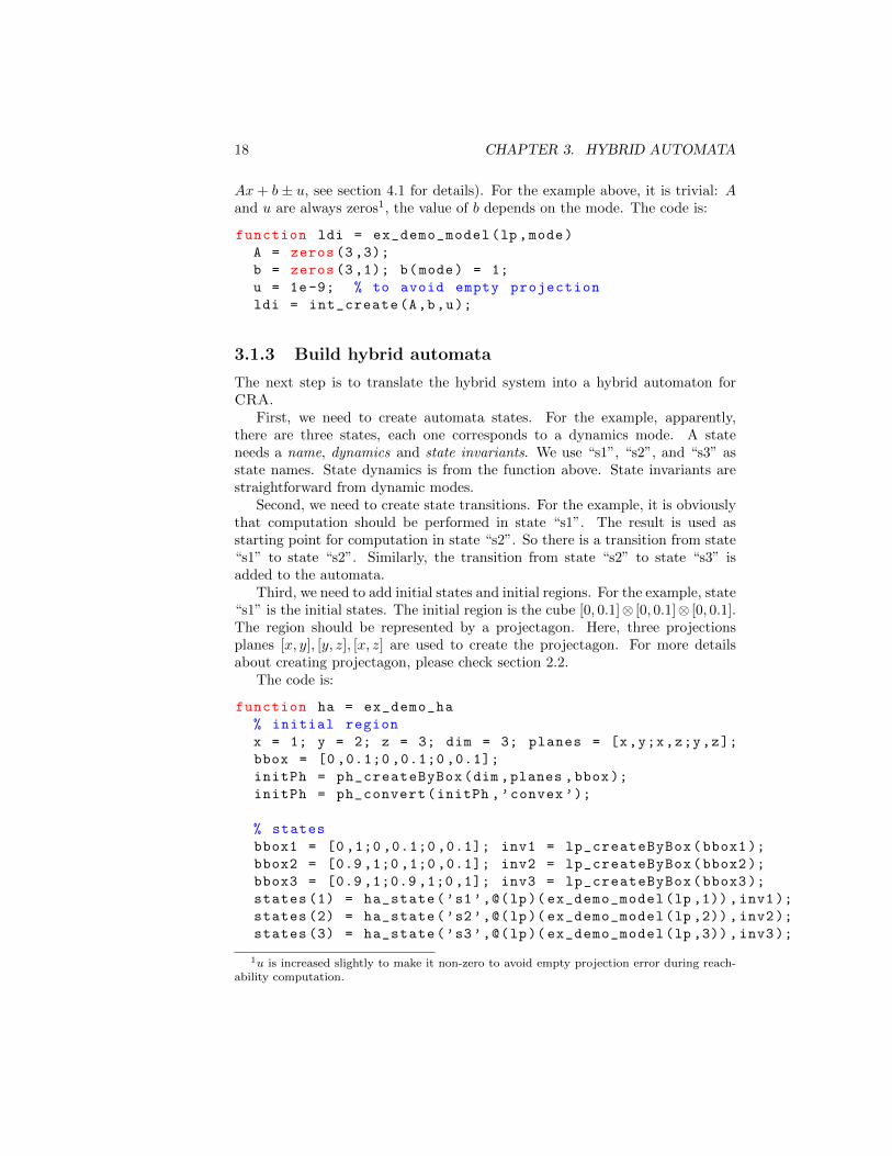
3.1.3 Build hybrid automata
The next step is to translate the hybrid system into a hybrid automaton forCRA.
First, we need to create automata states. For the example, apparently,there are three states, each one corresponds to a dynamics mode. A stateneeds a name, dynamics and state invariants. We use “s1”, “s2”, and “s3” asstate names. State dynamics is from the function above. State invariants arestraightforward from dynamic modes.
Second, we need to create state transitions. For the example, it is obviouslythat computation should be performed in state “s1”. The result is used asstarting point for computation in state “s2”. So there is a transition from state“s1” to state “s2”. Similarly, the transition from state “s2” to state “s3” isadded to the automata.
Third, we need to add initial states and initial regions. For the example, state“s1” is the initial states. The initial region is the cube [0, 0.1]⊗ [0, 0.1]⊗ [0, 0.1].The region should be represented by a projectagon. Here, three projectionsplanes [x, y], [y, z], [x, z] are used to create the projectagon. For more detailsabout creating projectagon, please check section 2.2.
The code is:
function ha = ex_demo_ha
% initial region
x = 1; y = 2; z = 3; dim = 3; planes = [x,y;x,z;y,z];
bbox = [0 ,0.1;0 ,0.1;0 ,0.1];
initPh = ph_createByBox(dim ,planes ,bbox);
initPh = ph_convert(initPh ,’convex ’);
% states
bbox1 = [0 ,1;0 ,0.1;0 ,0.1]; inv1 = lp_createByBox(bbox1 );
bbox2 = [0.9 ,1;0 ,1;0 ,0.1]; inv2 = lp_createByBox(bbox2 );
bbox3 = [0.9 ,1;0.9 ,1;0 ,1]; inv3 = lp_createByBox(bbox3 );
states (1) = ha_state(’s1’,@(lp)( ex_demo_model(lp ,1)), inv1);
states (2) = ha_state(’s2’,@(lp)( ex_demo_model(lp ,2)), inv2);
states (3) = ha_state(’s3’,@(lp)( ex_demo_model(lp ,3)), inv3);
1u is increased slightly to make it non-zero to avoid empty projection error during reach-ability computation.
3.2. HYBRID AUTOMATA 19
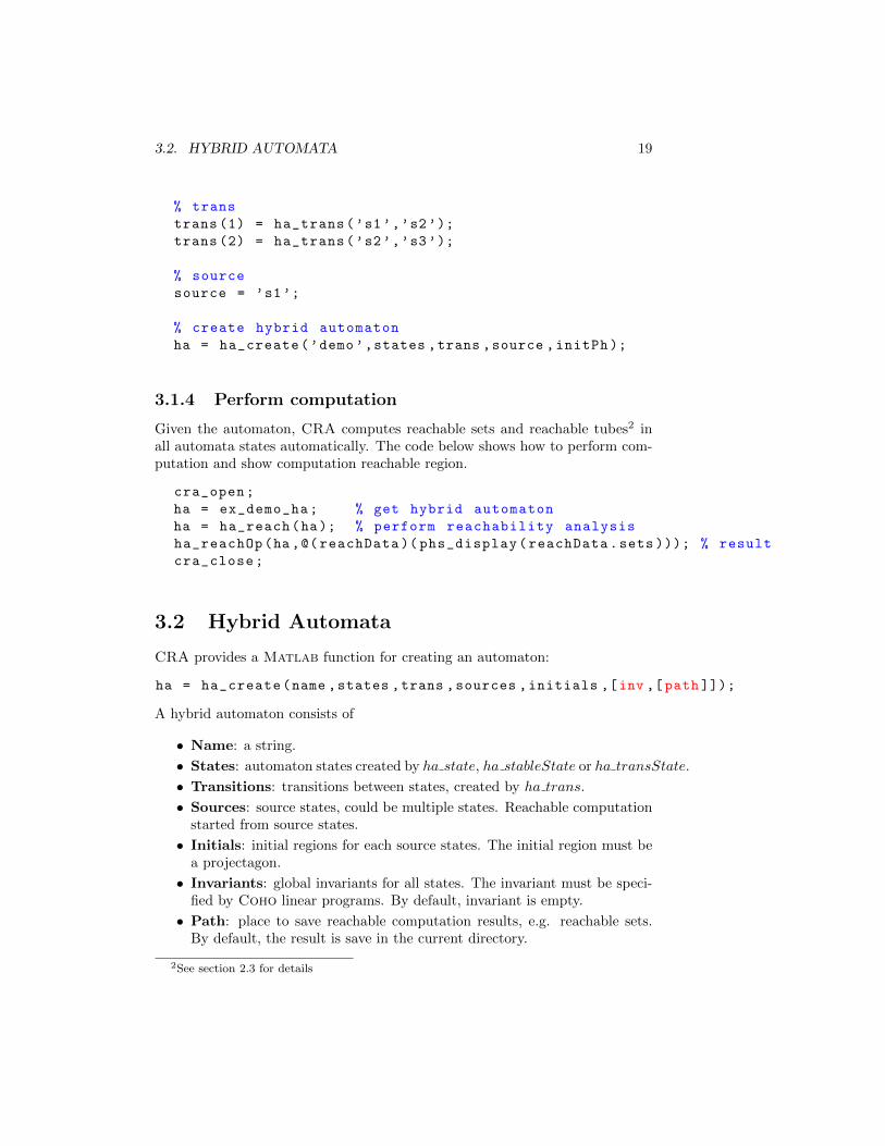
% trans
trans (1) = ha_trans(’s1’,’s2’);
trans (2) = ha_trans(’s2’,’s3’);
% source
source = ’s1’;
% create hybrid automaton
ha = ha_create(’demo’,states ,trans ,source ,initPh );
3.1.4 Perform computation
Given the automaton, CRA computes reachable sets and reachable tubes2 inall automata states automatically. The code below shows how to perform com-putation and show computation reachable region.
cra_open;
ha = ex_demo_ha; % get hybrid automaton
ha = ha_reach(ha); % perform reachability analysis
ha_reachOp(ha,@(reachData )( phs_display(reachData.sets ))); % result
cra_close;
3.2 Hybrid Automata
CRA provides a Matlab function for creating an automaton:
ha = ha_create(name ,states ,trans ,sources ,initials ,[inv ,[path ]]);
A hybrid automaton consists of
• Name: a string.
• States: automaton states created by ha state, ha stableState or ha transState.
• Transitions: transitions between states, created by ha trans.
• Sources: source states, could be multiple states. Reachable computationstarted from source states.
• Initials: initial regions for each source states. The initial region must bea projectagon.
• Invariants: global invariants for all states. The invariant must be speci-fied by Coho linear programs. By default, invariant is empty.
• Path: place to save reachable computation results, e.g. reachable sets.By default, the result is save in the current directory.
2See section 2.3 for details
20 CHAPTER 3. HYBRID AUTOMATA
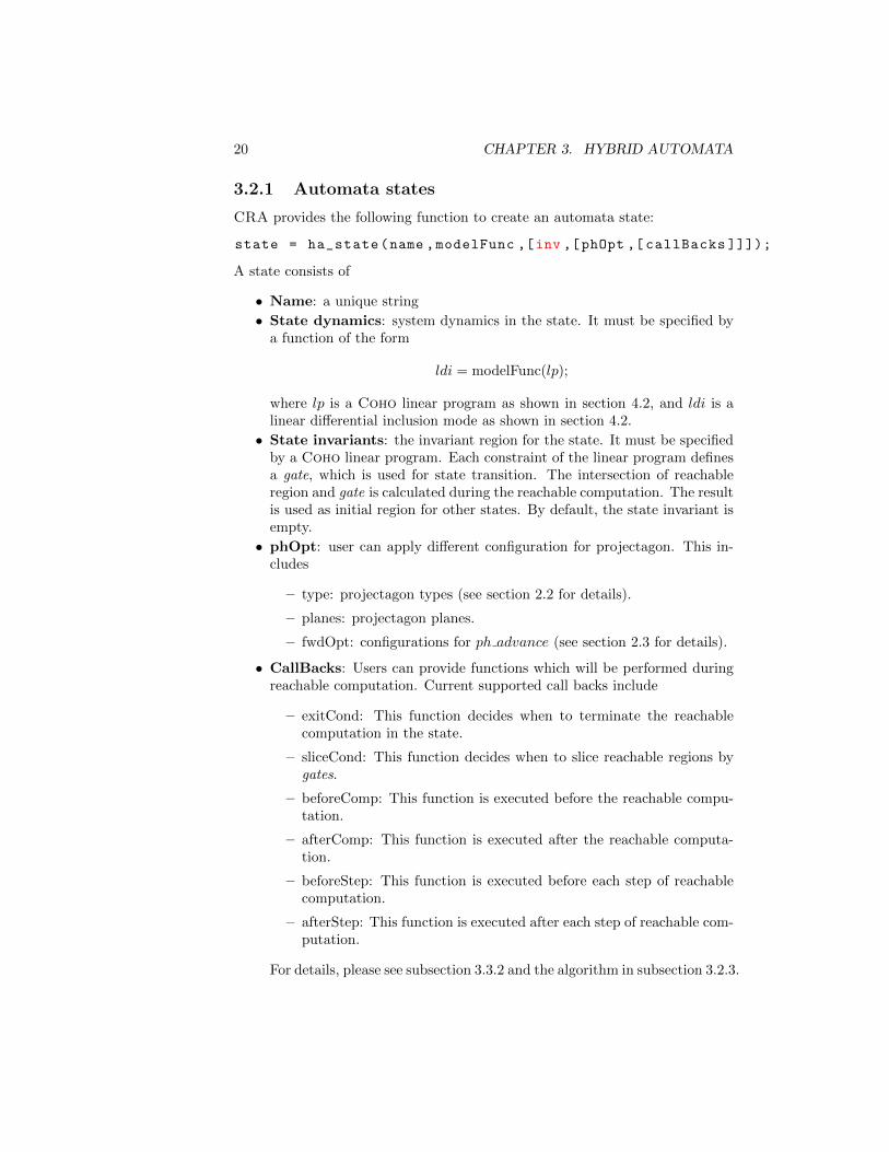
3.2.1 Automata states
CRA provides the following function to create an automata state:
state = ha_state(name ,modelFunc ,[inv ,[phOpt ,[ callBacks ]]]);
A state consists of
• Name: a unique string
• State dynamics: system dynamics in the state. It must be specified bya function of the form
ldi = modelFunc(lp);
where lp is a Coho linear program as shown in section 4.2, and ldi is alinear differential inclusion mode as shown in section 4.2.
• State invariants: the invariant region for the state. It must be specifiedby a Coho linear program. Each constraint of the linear program definesa gate, which is used for state transition. The intersection of reachableregion and gate is calculated during the reachable computation. The resultis used as initial region for other states. By default, the state invariant isempty.
• phOpt: user can apply different configuration for projectagon. This in-cludes
– type: projectagon types (see section 2.2 for details).
– planes: projectagon planes.
– fwdOpt: configurations for ph advance (see section 2.3 for details).
• CallBacks: Users can provide functions which will be performed duringreachable computation. Current supported call backs include
– exitCond: This function decides when to terminate the reachablecomputation in the state.
– sliceCond: This function decides when to slice reachable regions bygates.
– beforeComp: This function is executed before the reachable compu-tation.
– afterComp: This function is executed after the reachable computa-tion.
– beforeStep: This function is executed before each step of reachablecomputation.
– afterStep: This function is executed after each step of reachable com-putation.
For details, please see subsection 3.3.2 and the algorithm in subsection 3.2.3.
3.2. HYBRID AUTOMATA 21
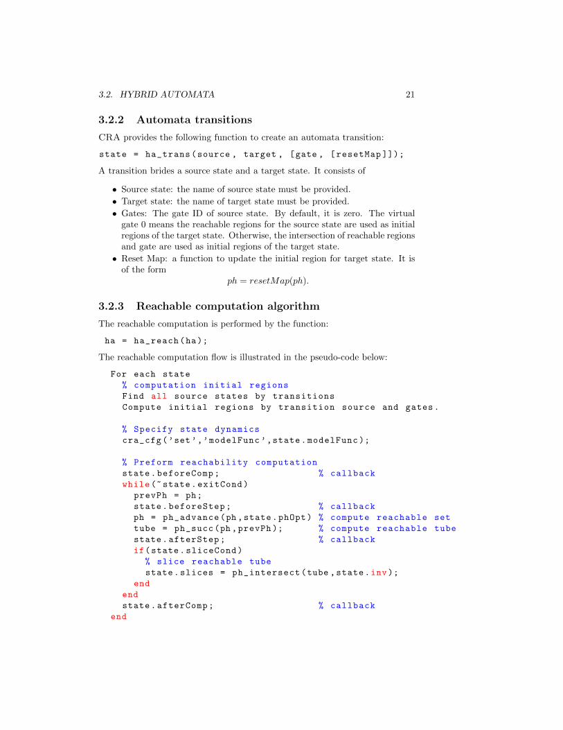
3.2.2 Automata transitions
CRA provides the following function to create an automata transition:
state = ha_trans(source , target , [gate , [resetMap ]]);
A transition brides a source state and a target state. It consists of
• Source state: the name of source state must be provided.
• Target state: the name of target state must be provided.
• Gates: The gate ID of source state. By default, it is zero. The virtualgate 0 means the reachable regions for the source state are used as initialregions of the target state. Otherwise, the intersection of reachable regionsand gate are used as initial regions of the target state.
• Reset Map: a function to update the initial region for target state. It isof the form
ph = resetMap(ph).
3.2.3 Reachable computation algorithm
The reachable computation is performed by the function:
ha = ha_reach(ha);
The reachable computation flow is illustrated in the pseudo-code below:
For each state
% computation initial regions
Find all source states by transitions
Compute initial regions by transition source and gates.
% Specify state dynamics
cra_cfg(’set’,’modelFunc ’,state.modelFunc );
% Preform reachability computation
state.beforeComp; % callback
while(~ state.exitCond)
prevPh = ph;
state.beforeStep; % callback
ph = ph_advance(ph ,state.phOpt) % compute reachable set
tube = ph_succ(ph ,prevPh ); % compute reachable tube
state.afterStep; % callback
if(state.sliceCond)
% slice reachable tube
state.slices = ph_intersect(tube ,state.inv);
end
end
state.afterComp; % callback
end
22 CHAPTER 3. HYBRID AUTOMATA
% save all reachable data onto disk
3.3 Advanced Configuration
3.3.1 Performance v.s Accuracy
Obtaining a good balance between performance and accuracy is an importantstep for many reachability analysis problems. CRA provides several options tocontrol performance and accuracy.
Reachability computation in each automata state could be specified individ-ually by setting the parameter pOpt. It includes
• phOpt.type: Users can use different projectagon types in automata states.Generally speaking, convex projectagon are suitable in most case. Non-convex projectagon are use to optimize accuracy with slower computation.Bounding box projectagon have bad accuracy, may only suitable for ex-tremely simple problems.
• phOpt.plane: Users can specify projectagon planes for each automatastate. For a n-dimensional system, the number of planes is in the range of[n− 1, n(n− 1)/2]. Generally speaking, the more planes used, the betteraccuracy is the computation result with the cost of more computationtime. Usually, if dynamics of xi and xj highly depends on each others, itis recommended to include the plane xi, xj to get better accuracy.
• phOpt.fwdOpt.model: User can specify the way to compute advance timestep. Usually, the default value of guess verify provides better perfor-mance and accuracy. For more details, please check section 2.3.
• phOpt.fwdOpt.object: Generally speaking, ph is much faster than othermethods with relatively larger error than face-none,face-bloat,face-height.The performance of face-none,face-bloat and face-height are similar.Face-none has less error than the other two methods, but doesn’t guar-antee soundness as the other two method do. Note face-none requiresthat the error term of the linear differential inclusion model provided byusers can not be zeros. Face-height usually has slightly smaller errorthan face-bloat, especially for high-dimensional system. Face-all hasthe largest error and slowest computation, it’s not recommended to beused by users. For more details, please check section 2.3.
Slicing is a useful method to reduce error and improve performance. Usually,if a variable x changes rapidly in large range [xl, xh] monotonically, slicing thevariable into smaller intervals helps to reduce accumulated error and improveperformance. Of course, the number of hybrid automata states increase, thuscould increase total running time.
Linearization error is an important part of computation error. It is highlyrecommended to reduce the error term of the linear differential inclusion modelcomputed in the user-provided function as possible. Employing multiple models
3.4. FUNCTIONS 23
can also reduce linearization error to obtain more accurate result. However, thisusually increases the computation time.
3.3.2 Callbacks
Callbacks provide user the ability to execute their own Matlab functions duringreachability computation. During reachability computation in each state, userscan provide functions
• exitCond: Condition to terminate the reachability computation in thestate. It is of the format: exitCond = exitCond(info), where info is astructure with fields ”ph”,”prevPh”,”fwdStep”,”fwdT”,’compT”.
• sliceCond: Condition to slice reachable tubes with invariant faces/gates.It s of the format: sliceCond = sliceCond(info), where ”info” has fields”complete”, ”ph”, ”prevPh”, ”fwdStep”, ”fwdT”, ”compT”.
• beforeComp: called before the reachability computation. It is of the for-mat: beforeComp(info), where info has fields ”initPh”.
• afterComp: called at the end of reachability computation. It is of the for-mat: afterComp(info), where info has the fields ”sets”,”tubes”,’timeSteps”,”faces”.
• beforeStep: called before each computation step. It is of the format: ph= beforeStep(info), where info has the following fields: ”ph”, ”prevPh”,”fwdStep”, ”fwdT”, ”compT”.
• afterStep: called after each computation step. It is of the format: ph= afterStep(info), where info has the fields: ”ph”, ”prevPh”, ”fwdStep”,”fwdT”, ”compT ”.
During state transitions, users can also provide functions to update initialregions.
To simplify the usage of call backs, CRA provides templates of callbacks by
func = ha_callBacks(callback , method , ...)
For example, displaying reachable regions after each computation step could bespecified by
callBacks.afterStep = ha_callBacks(’afterStep ’, ’display ’);
3.4 Functions
We list the main functions for users with short descriptions. For details, pleasecheck in Matlab help document.
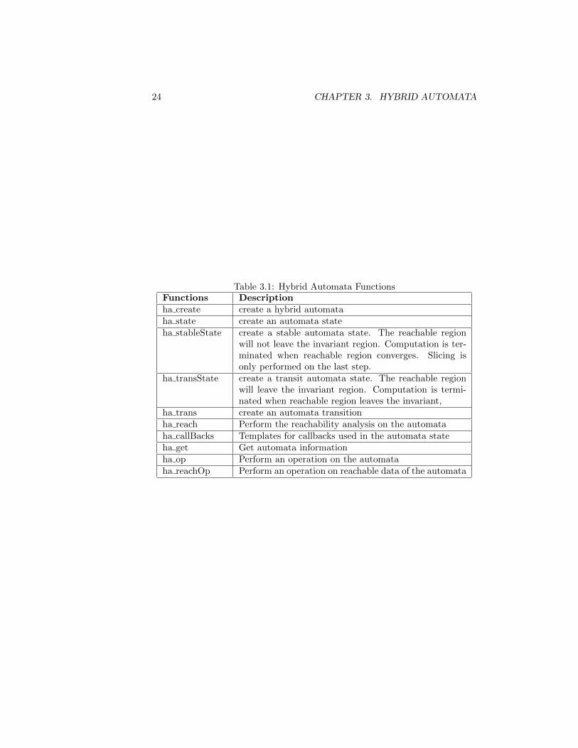
24 CHAPTER 3. HYBRID AUTOMATA
Table 3.1: Hybrid Automata FunctionsFunctions Descriptionha create create a hybrid automataha state create an automata stateha stableState create a stable automata state. The reachable region
will not leave the invariant region. Computation is ter-minated when reachable region converges. Slicing isonly performed on the last step.
ha transState create a transit automata state. The reachable regionwill leave the invariant region. Computation is termi-nated when reachable region leaves the invariant,
ha trans create an automata transitionha reach Perform the reachability analysis on the automataha callBacks Templates for callbacks used in the automata stateha get Get automata informationha op Perform an operation on the automataha reachOp Perform an operation on reachable data of the automata
Chapter 4
Others
4.1 Linear Differential Inclusion
CRA over-approximates system dynamics by linear differential inclusion on-the-fly. A linear differential inclusion is a structure with fields A, b, u, representinga inclusion of the form
x = Ax + b± u (4.1)
It is recommended to construct a linear differential inclusion by
ldi = int_create(A,b,u);
4.2 Linear Programming
CRA supports Coho linear programs of the form:
Ax ≤ b (4.2)
where A is a matrix with only one or two non-zero elements on each row. Coholinear programs corresponds to convex hull of projectagons. A Coho linearprogram can be constructed by
lp = lp_create(A,b);
CRA implements an efficient solver for Coho linear programs based onarbitrary precision rational numbers. Users can use the solver by
[optV ,optPt ,status] = lp_solve(lp,optDir );
Beside the built-in linear program solver, CRA also support Matlab built-in solver or the CPLEX solvers. These solvers (especially the CPLEX solver)could be faster than our solver which is implemented in Java. But thesesolvers suffer from numerical problems. CRA support hybrid method whichtries CPLEX (Matlab) solver first, and re-solves the problem by our Java if
25
26 CHAPTER 4. OTHERS
failed. The default linear program solver can be configured by users as shownin section 4.4.
CRA also implements a solver to project a Coho linear programs onto two-dimensional subspace. Users can use the solver by
hull = lp_project(lp ,planes );
CRA also implements another solver based on the Matlab linear programsolver. But it is not numerical stable, thus not recommend to use.
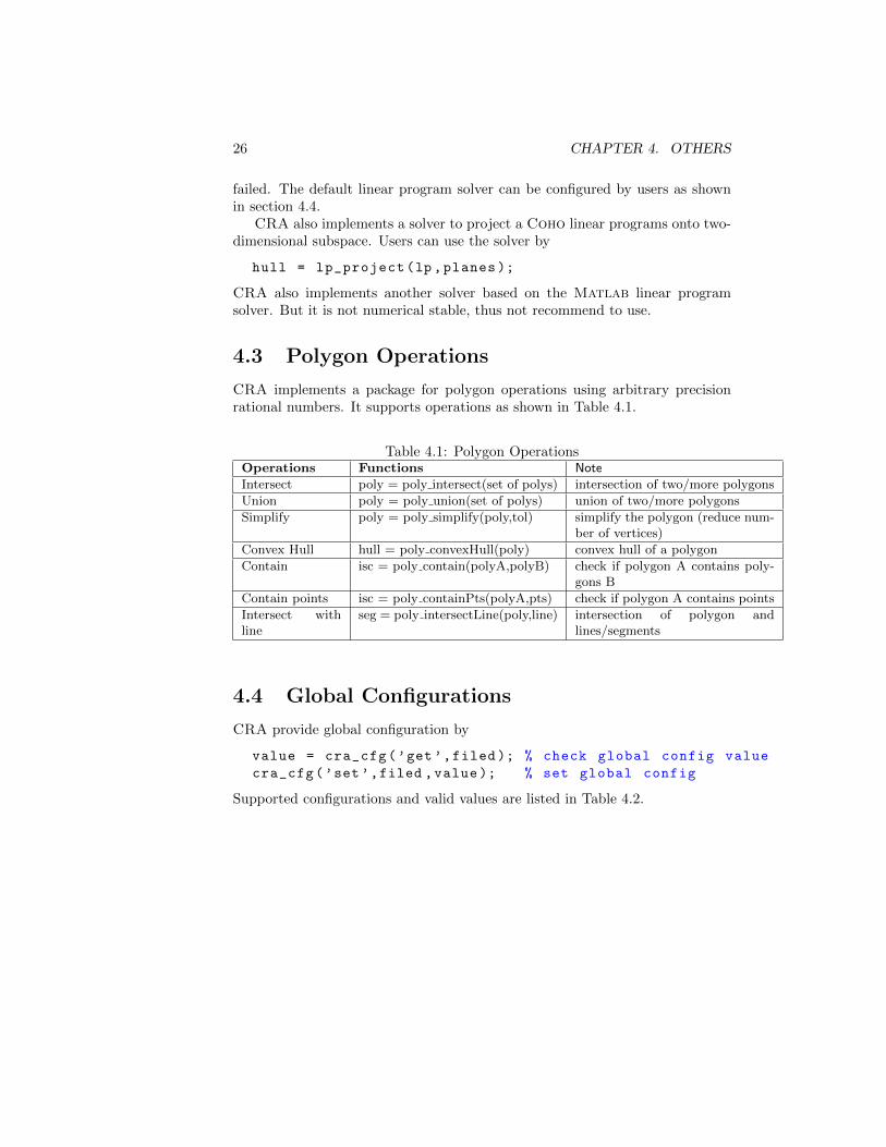
4.3 Polygon Operations
CRA implements a package for polygon operations using arbitrary precisionrational numbers. It supports operations as shown in Table 4.1.
Table 4.1: Polygon OperationsOperations Functions Note
Intersect poly = poly intersect(set of polys) intersection of two/more polygons
Union poly = poly union(set of polys) union of two/more polygons
Simplify poly = poly simplify(poly,tol) simplify the polygon (reduce num-ber of vertices)
Convex Hull hull = poly convexHull(poly) convex hull of a polygon
Contain isc = poly contain(polyA,polyB) check if polygon A contains poly-gons B
Contain points isc = poly containPts(polyA,pts) check if polygon A contains points
Intersect withline
seg = poly intersectLine(poly,line) intersection of polygon andlines/segments
4.4 Global Configurations
CRA provide global configuration by
value = cra_cfg(’get’,filed ); % check global config value
cra_cfg(’set’,filed ,value); % set global config
Supported configurations and valid values are listed in Table 4.2.
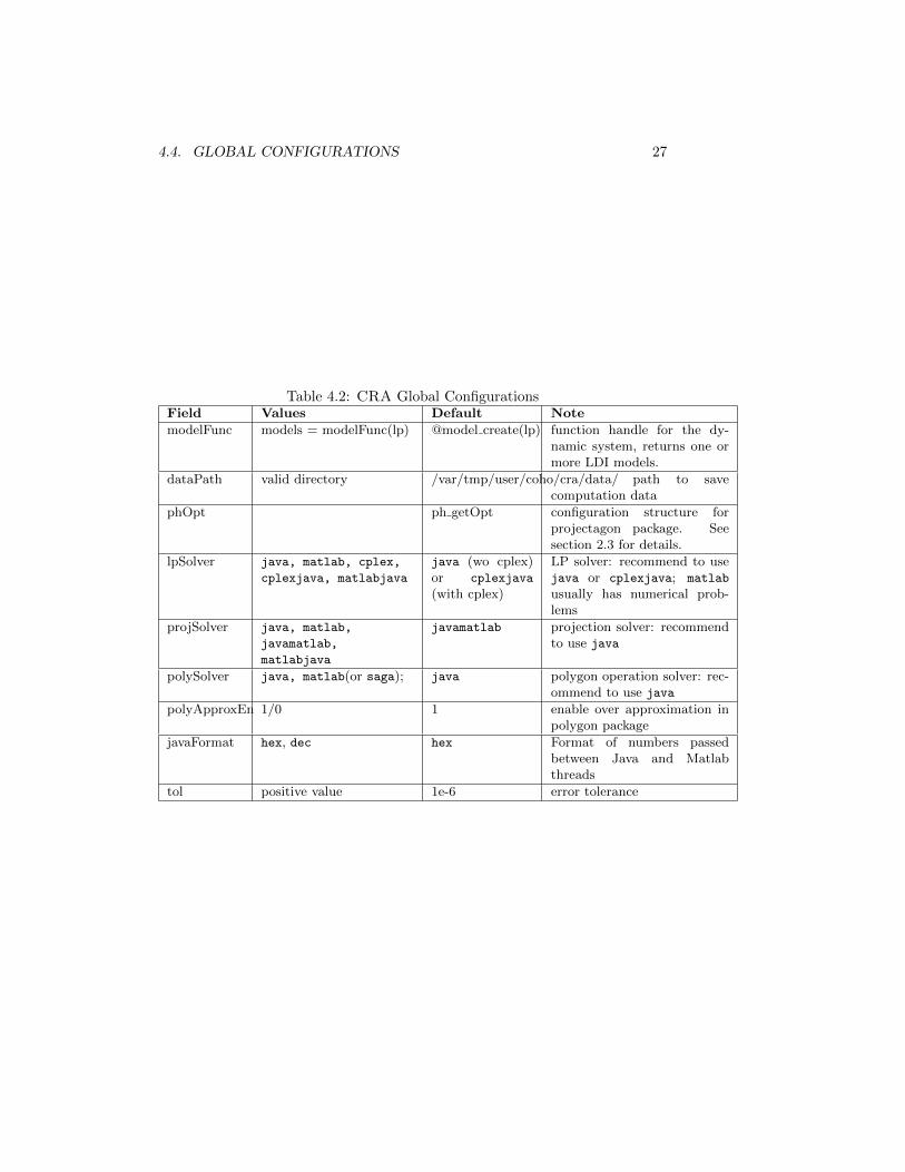
4.4. GLOBAL CONFIGURATIONS 27
Table 4.2: CRA Global ConfigurationsField Values Default Note
modelFunc models = modelFunc(lp) @model create(lp) function handle for the dy-namic system, returns one ormore LDI models.
dataPath valid directory /var/tmp/user/coho/cra/data/ path to savecomputation data
phOpt ph getOpt configuration structure forprojectagon package. Seesection 2.3 for details.
lpSolver java, matlab, cplex,
cplexjava, matlabjava
java (wo cplex)or cplexjava
(with cplex)
LP solver: recommend to usejava or cplexjava; matlab
usually has numerical prob-lems
projSolver java, matlab,
javamatlab,
matlabjava
javamatlab projection solver: recommendto use java
polySolver java, matlab(or saga); java polygon operation solver: rec-ommend to use java
polyApproxEn 1/0 1 enable over approximation inpolygon package
javaFormat hex, dec hex Format of numbers passedbetween Java and Matlabthreads
tol positive value 1e-6 error tolerance

28 CHAPTER 4. OTHERS

Chapter 5
Examples
CRA has been applied to solve problems listed in Table 5.1.
Table 5.1: CRA ExamplesProblem Code Dim Source Note
Sink ex 2sink 2 [6] Two dimensional sink example
TDO ex 2tdo 2 [4] Tunnel Diode Oscillator circuit
VDP2 ex 2vdp 2 [3] Two dimensional Van der Pol oscillator
VDP3 ex 3vdp 3 [6] Three dimensional Van der Pol oscillator
DM ex 3dm 3 [3] Dang and Maler’s example
PD ex 3pd 3 [3] Play-Doh example
VCO ex 3vco 3 [1] Voltage controlled oscillator circuit
PLL ex 3pll 3 [5] A digital PLL circuit
29

30 CHAPTER 5. EXAMPLES
Bibliography
[1] Goran Frehse, Bruce H. Krogh, and Rob A. Rutenbar. Verifying ana-log oscillator circuits using forward/backward abstraction refinement. InDATE ’06: Proceedings of the conference on Design, automation and testin Europe, pages 257–262, 3001 Leuven, Belgium, Belgium, 2006. EuropeanDesign and Automation Association. 29
[2] Mark R. Greenstreet and Ian Mitchell. Integrating projections. In HSCC’98: Proceedings of the First International Workshop on Hybrid Systems,pages 159–174. Springer Verlag, 1998. 5, 7, 10
[3] Mark R. Greenstreet and Ian Mitchell. Reachability analysis using polyg-onal projections. In HSCC ’99: Proceedings of the Second InternationalWorkshop on Hybrid Systems, pages 103–116, London, UK, 1999. Springer-Verlag. 5, 7, 29
[4] Smriti Gupta, Bruce H. Krogh, and Rob A. Rutenbar. Towards formalverification of analog designs. In Proceedings of 2004 IEEE/ACM Inter-national Conference on Computer Aided Design, pages 210–217, November2004. 29
[5] Jijie Wei, Mark R. Greenstreet, Yan Peng, and Ge Yu. Verifying globalconvergence for a digital phase-locked loop. In FMCAD13, 2013. 29
[6] Chao Yan. Coho: A verification tool for circuit verification by reachabilityanalysis. Master’s thesis, The University of British Columbia, August 2006.7, 29
[7] Chao Yan. Reachability Analysis Based Circuit-Level Formal Verification.PhD thesis, The University of British Columbia, 2011. 5, 7, 10
[8] Chao Yan. Coho circuit modeling (coho-reach) tool manual. 2014. 7
[9] Chao Yan and Mark R. Greenstreet. Circuit level verification of a high-speed toggle. In FMCAD, pages 199–206, Washington, DC, USA, Novem-ber 2007. IEEE Computer Society. 7
[10] Chao Yan and Mark R. Greenstreet. Faster projection based methods forcircuit level verification. In ASP-DAC, pages 410–415, Los Alamitos, CA,USA, January 2008. IEEE Computer Society Press. 7
31
32 BIBLIOGRAPHY
[11] Chao Yan and Mark R. Greenstreet. Verifying an arbiter circuit. In Alessan-dro Cimatti and Robert B. Jones, editors, FMCAD, pages 1–9, Piscataway,NJ, USA, November 2008. IEEE Press. 7
[12] Chao Yan and Mark R Greenstreet. Oscillator verification with probabilityone. In Jason Baumgartner and Mary Sheeran, editors, FMCAD, pages165–172. IEEE Press, October 2012. 7
[13] Chao Yan, Mark R. Greenstreet, and Jochen Eisinger. Formal verificationof arbiters. The 16th IEEE International Symposium on AsynchronousCircuits and Systems, May 2010. 7
[14] Chao Yan, Mark R. Greenstreet, and Marius Laza. A robust linear programsolver for reachability analysis. In Proceedings of the First InternationalConference on Mathematical Aspects of Computer and Information Sci-ences (MACIS), pages pp231–242, Beijing, China, July 2006. 7
[15] Chao Yan, MarkR. Greenstreet, and Suwen Yang. Verifying global start-upfor a mbius ring-oscillator. Formal Methods in System Design, pages 1–27,2013. 7
[16] Chao Yan, Florent Ouchet, Laurent Fesquet, and Katell Morin-Allory. For-mal verification of c-element circuits. The 17th IEEE International Sym-posium on Asynchronous Circuits and Systems, April 2011. 7