Coherent structures in wall turbulence

Short term goal: understand and control near wall processes (relevant for drag, lift, resuspension, etc)Long term goal: shift turbulent closure to larger scales, in order to solve large domain accurately (atmosphere, rivers, oceans)

Smallest scale of the flow: kolmogorov scale (in the near atmosphere about 1mm)

Largest scale of the flow: several times the boundary layer height(in the atmosphere may go up to O(1-10 Km )

There are 6-7 orders of magnitude !

However IF, we understand how turbulent structures behave and IFthese structures truly play a major role (statistically) on momentum, scalar and energy fluxes, mixing, etc. ...Then we could propose low dimensional models, smart closures, control systems

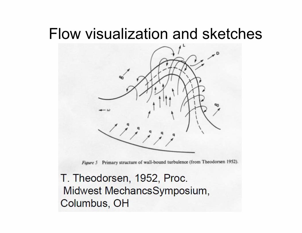
Flow visualization and sketches

Kline 1967 (near wall streaks) (log and outer layer)

(1981)

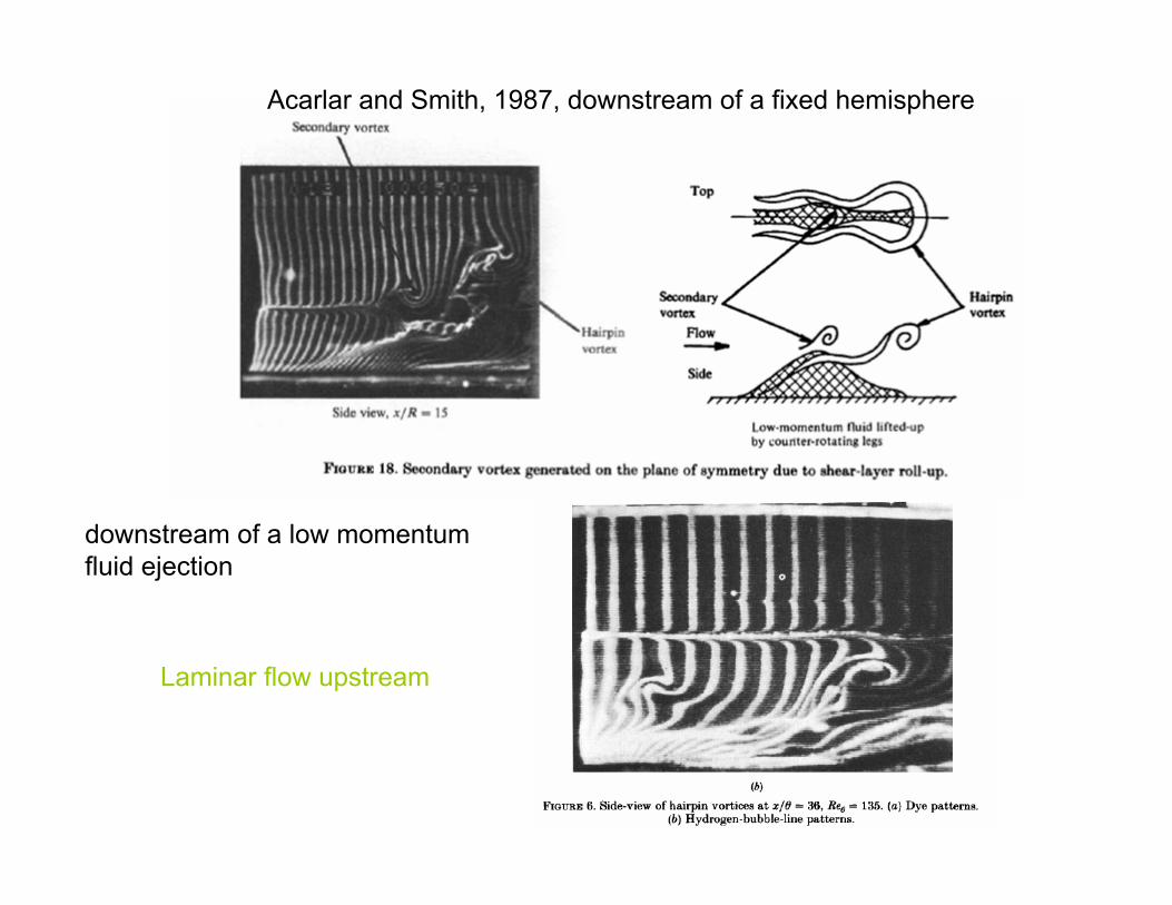
Acarlar and Smith, 1987, downstream of a fixed hemisphere

downstream of a low momentum fluid ejection

Laminar flow upstream

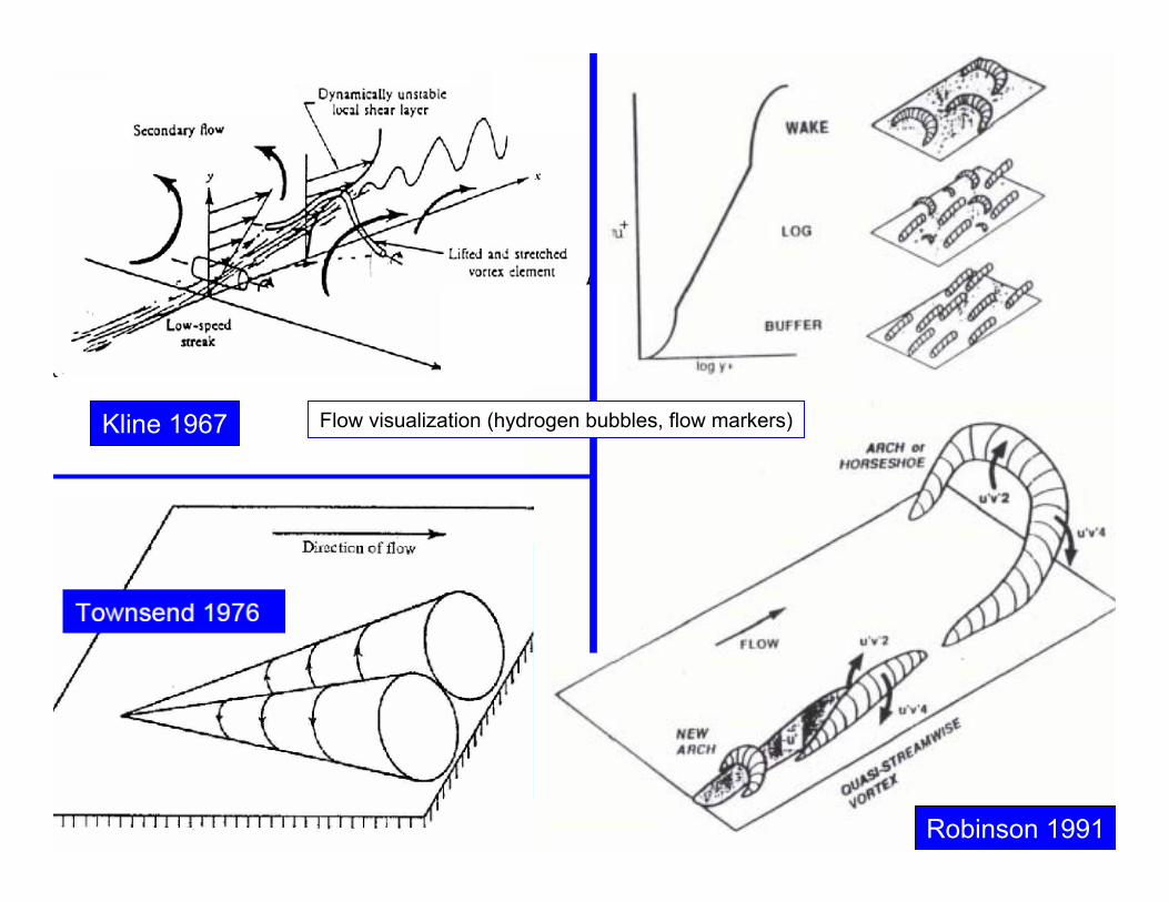
Robinson 1991

Kline 1967 Flow visualization (hydrogen bubbles, flow markers)

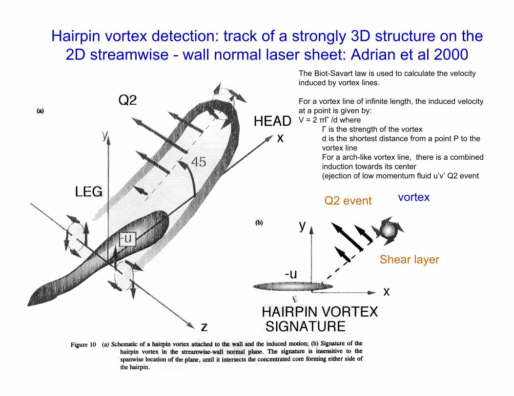
Hairpin vortex detection: track of a strongly 3D structure on the 2D streamwise - wall normal laser sheet: Adrian et al 2000

vortexQ2 event

Shear layer

The Biot-Savart law is used to calculate the velocity induced by vortex lines.

For a vortex line of infinite length, the induced velocity at a point is given by:V = 2 πΓ /d where

Γ is the strength of the vortexd is the shortest distance from a point P to the vortex lineFor a arch-like vortex line, there is a combined induction towards its center (ejection of low momentum fluid u’v’ Q2 event

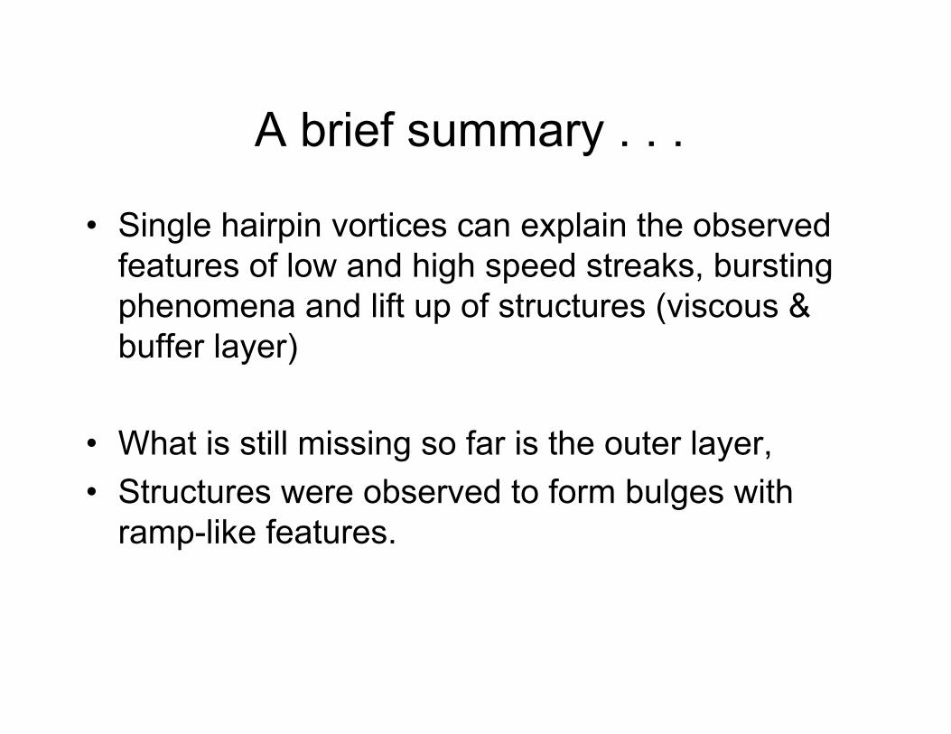
• Single hairpin vortices can explain the observed features of low and high speed streaks, bursting phenomena and lift up of structures (viscous & buffer layer)

• What is still missing so far is the outer layer,• Structures were observed to form bulges with

ramp-like features.

A brief summary . . .

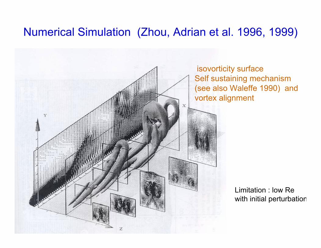
Numerical Simulation (Zhou, Adrian et al. 1996, 1999)

isovorticity surfaceSelf sustaining mechanism(see also Waleffe 1990) and vortex alignment

Limitation : low Re with initial perturbation

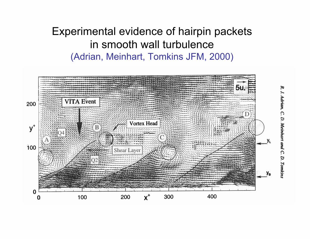
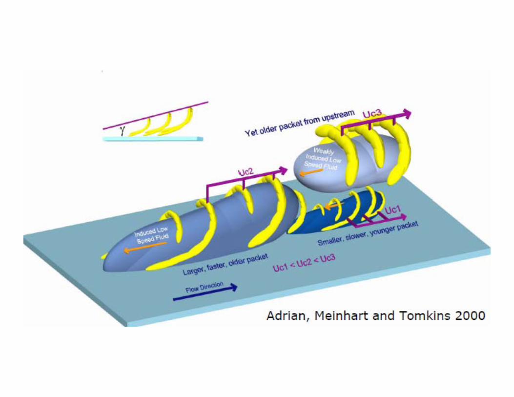
Experimental evidence of hairpin packets in smooth wall turbulence

(Adrian, Meinhart, Tomkins JFM, 2000)

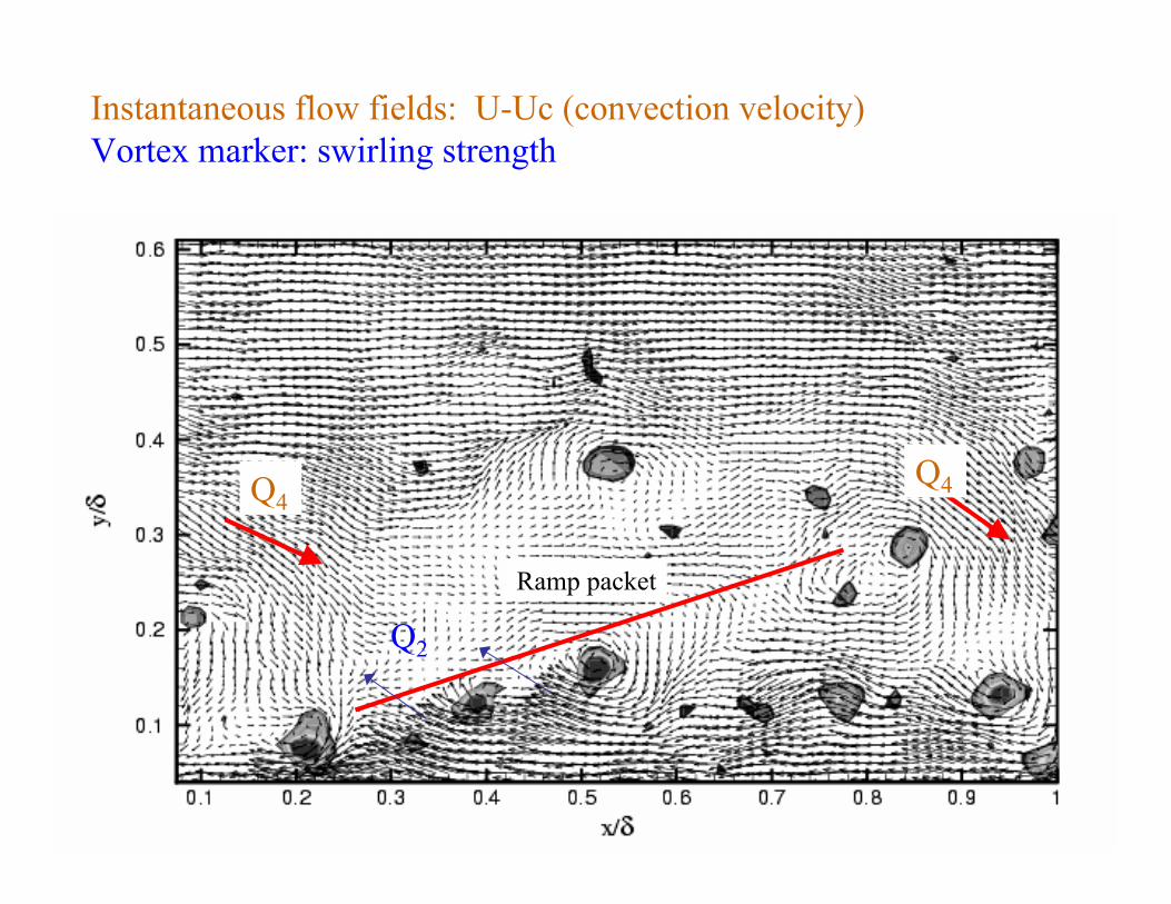
Instantaneous flow fields: U-Uc (convection velocity) Vortex marker: swirling strength

Ramp packet

Q2

Q4Q4

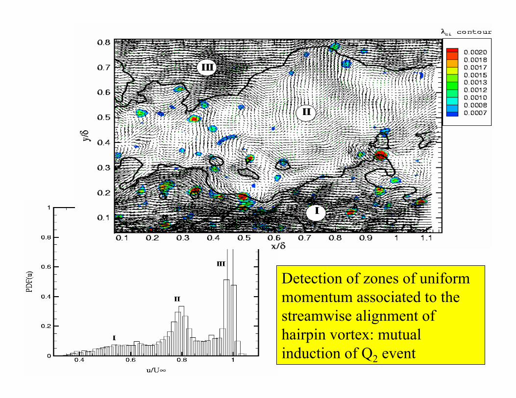
Detection of zones of uniform momentum associated to the streamwise alignment of hairpin vortex: mutual induction of Q2 event

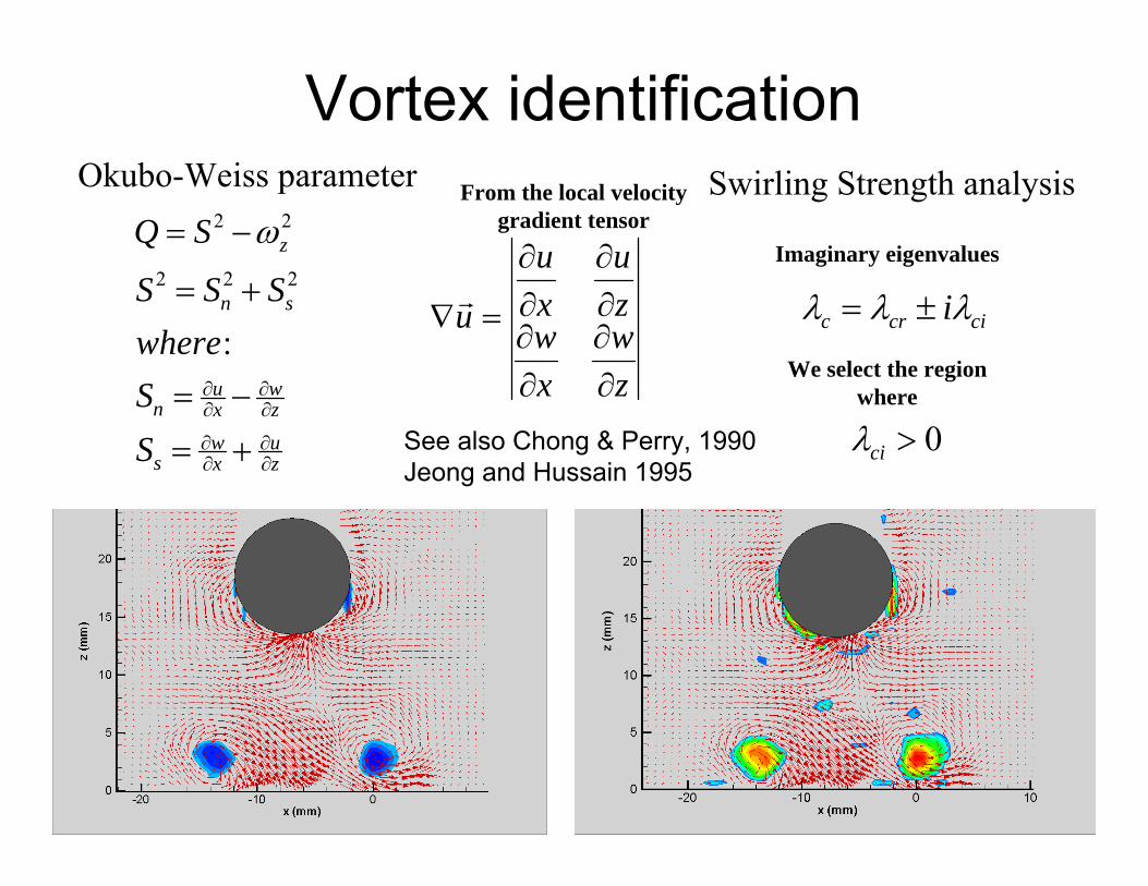
Vortex identificationOkubo-Weiss parameter Swirling Strength analysis

zu

xw

s

zw

xu

n

sn

SSwhere

SSS

:

222

22zSQ

zw

xw

zu

xu

u

From the local velocity gradient tensor

Imaginary eigenvalues

cicrc i

We select the region where

0ciSee also Chong & Perry, 1990Jeong and Hussain 1995

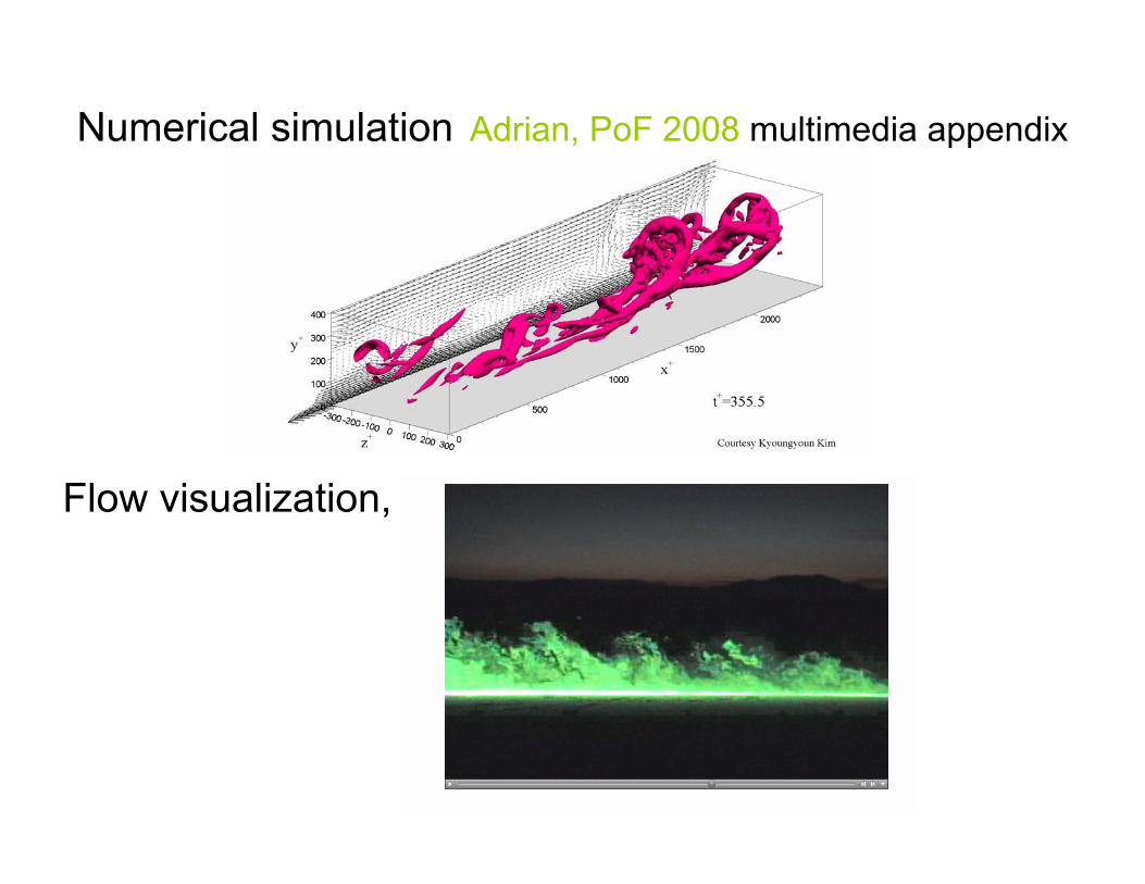
Numerical simulation Adrian, PoF 2008 multimedia appendix

Flow visualization,

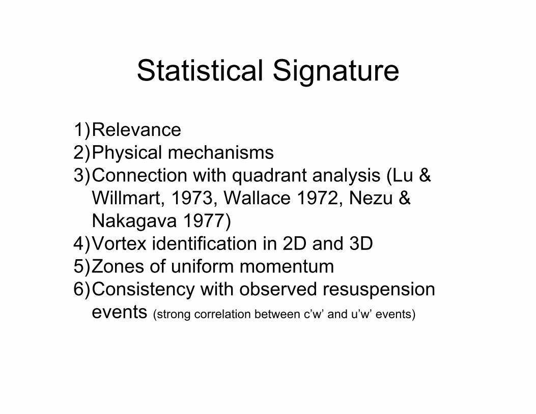
Statistical Signature

1)Relevance 2)Physical mechanisms3)Connection with quadrant analysis (Lu &

Willmart, 1973, Wallace 1972, Nezu & Nakagava 1977)

4)Vortex identification in 2D and 3D5)Zones of uniform momentum6)Consistency with observed resuspension

events (strong correlation between c’w’ and u’w’ events)

Besides instantaneous realizations…Is it possible to obtain some quantitative information about turbulent structures ?

2 point correlation

vu, ji,for

y'σyσ',,

ρ

d)(normalizet coefficienn correlatio

', ,',,

n tensorcorrelatiopoint 2

jiij

*

yyrR

yrxuyxuyyrR

xij

xjixij

Linear stochastic estimate

Estimate of the flow fieldStatistically conditionedTo the realization of a known event :

1) II quadrant (u < 0, v > 0)2) IV quadrant (u > 0, v < 0)3) Vortex

identified by the swirling strength complex part of the eigenvalue of the local velocity gradient tensor.

See also Proper Orthogonal Decomposition (Holmes & Lumley )

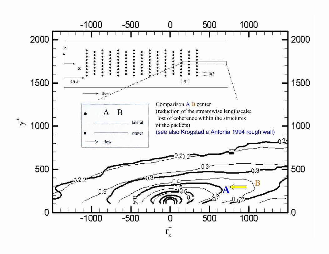
AB

Comparison A B center (reduction of the streamwise lengthscale:lost of coherence within the structures of the packets) (see also Krogstad e Antonia 1994 rough wall)

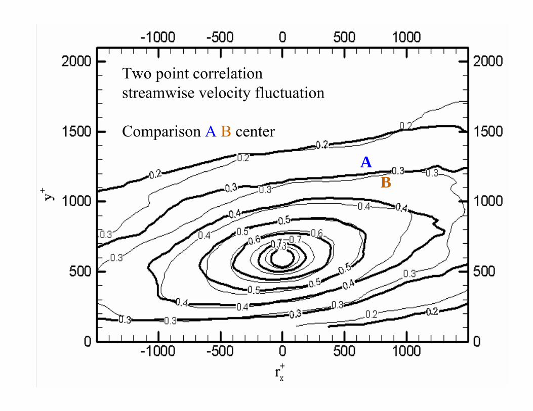
Two point correlationstreamwise velocity fluctuation

Comparison A B center

BA

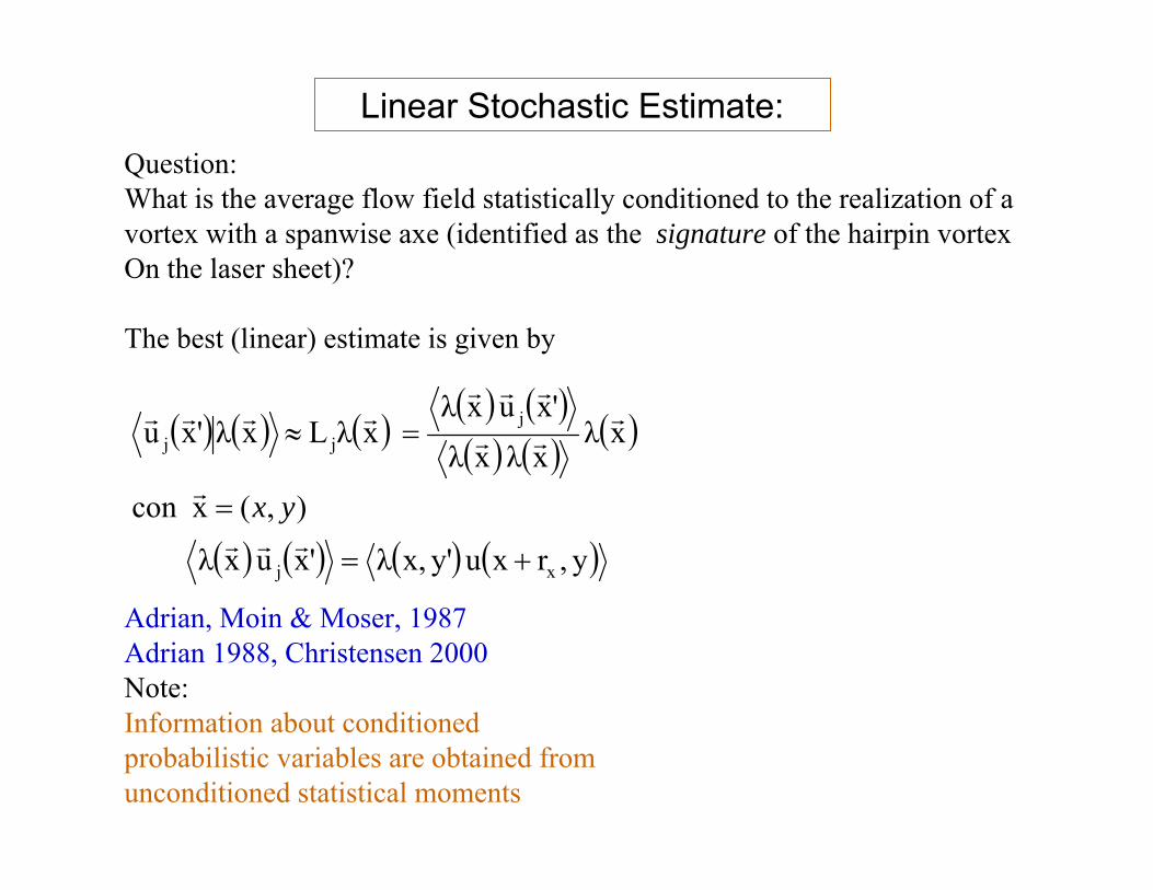
Linear Stochastic Estimate:Question:What is the average flow field statistically conditioned to the realization of a vortex with a spanwise axe (identified as the signature of the hairpin vortexOn the laser sheet)?

The best (linear) estimate is given by

Adrian, Moin & Moser, 1987 Adrian 1988, Christensen 2000Note:Information about conditioned probabilistic variables are obtained from unconditioned statistical moments

y,rxu y'x,λ'xu xλ

),(xcon

xλxλ xλ

'xu xλ xλL xλ'xu

xj

jjj

yx

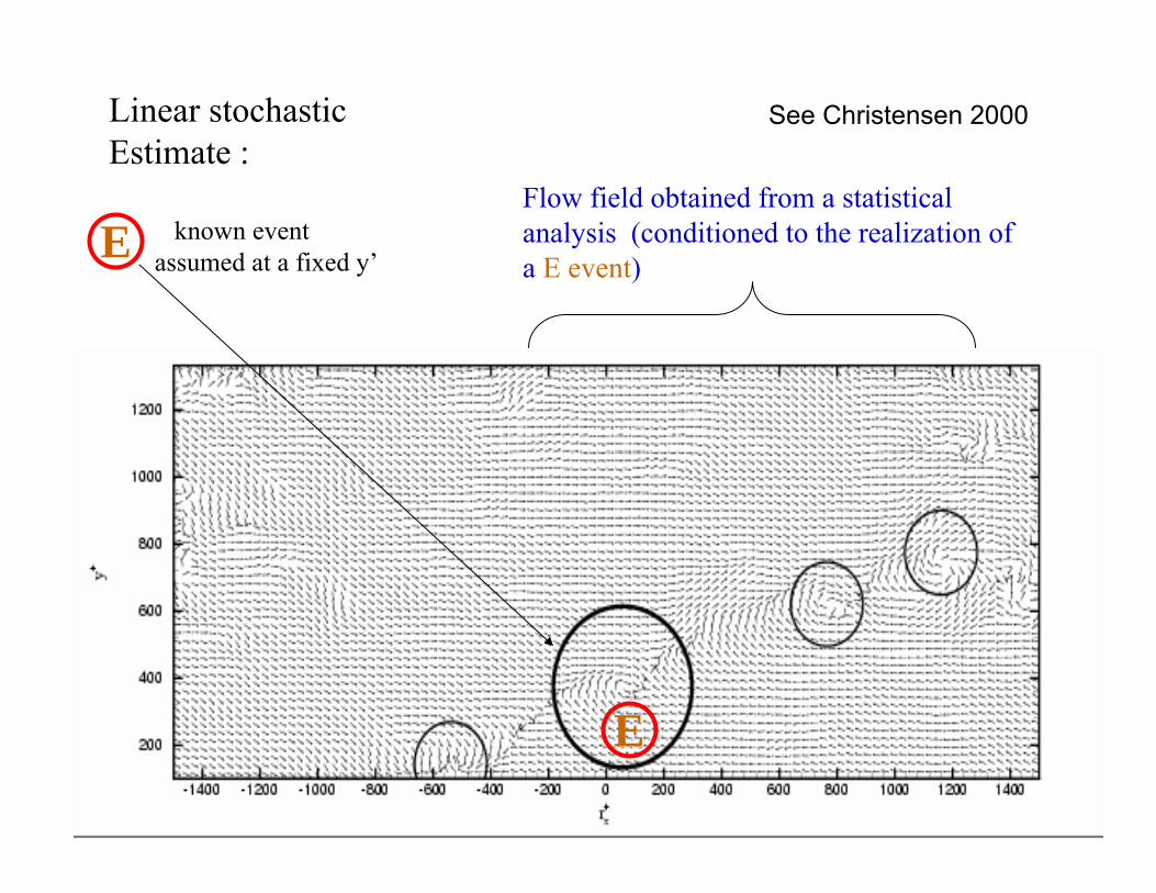
Linear stochasticEstimate :

known event assumed at a fixed y’

Flow field obtained from a statistical analysis (conditioned to the realization of a E event)

E

E

See Christensen 2000

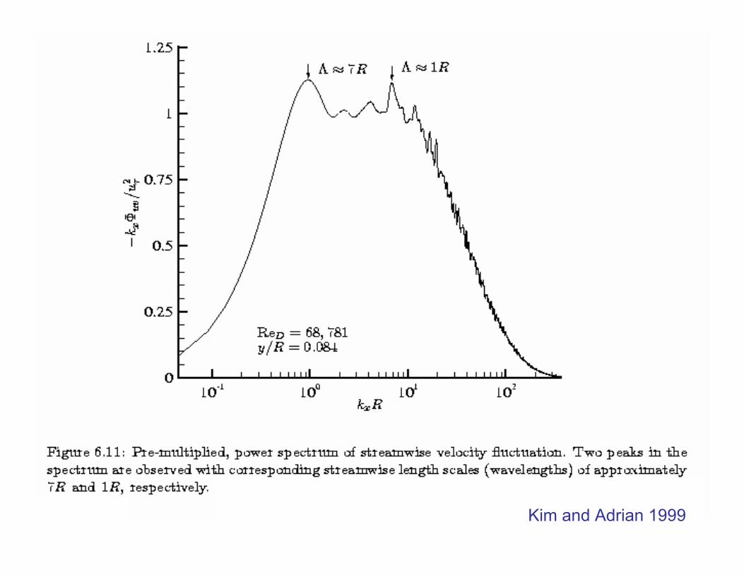
Kim and Adrian 1999

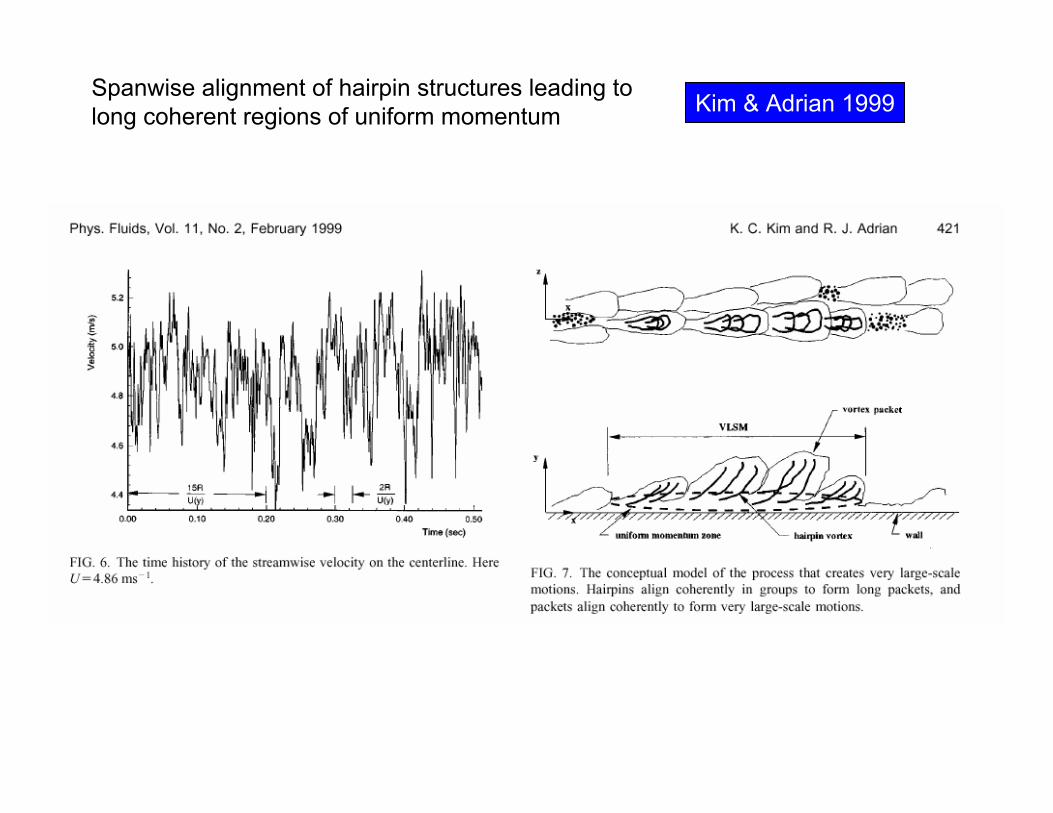
Spanwise alignment of hairpin structures leading to long coherent regions of uniform momentum Kim & Adrian 1999

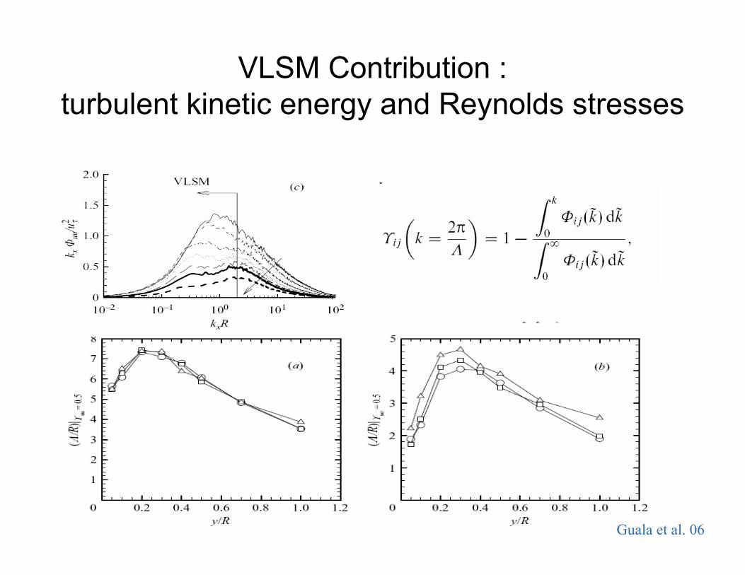
VLSM Contribution : turbulent kinetic energy and Reynolds stresses

Guala et al. 06

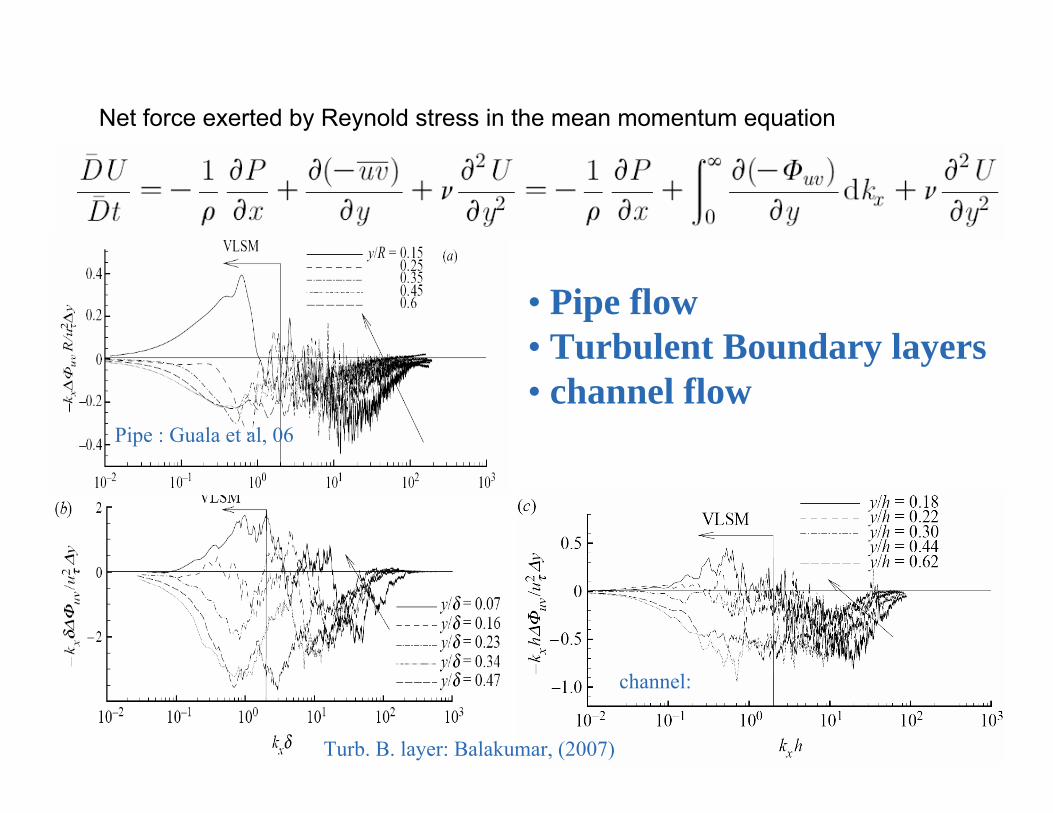
Pipe : Guala et al, 06

channel:

• Pipe flow• Turbulent Boundary layers • channel flow

Turb. B. layer: Balakumar, (2007)

Net force exerted by Reynold stress in the mean momentum equation

• Large scale motion participate significantly to the Reynolds stress, thus contribute not only to TKE but also to TKE production.

• In terms of momentum balance, close to the wall, VLSM push the flow forward, while smaller scales slow down the flow.

• Such features are observed for turbulent pipe, channel and boundary layers flows

A brief summary . . .

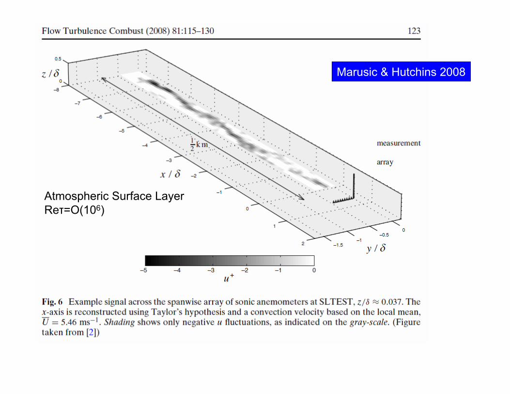
Marusic & Hutchins 2008

Atmospheric Surface LayerReτ=O(106)

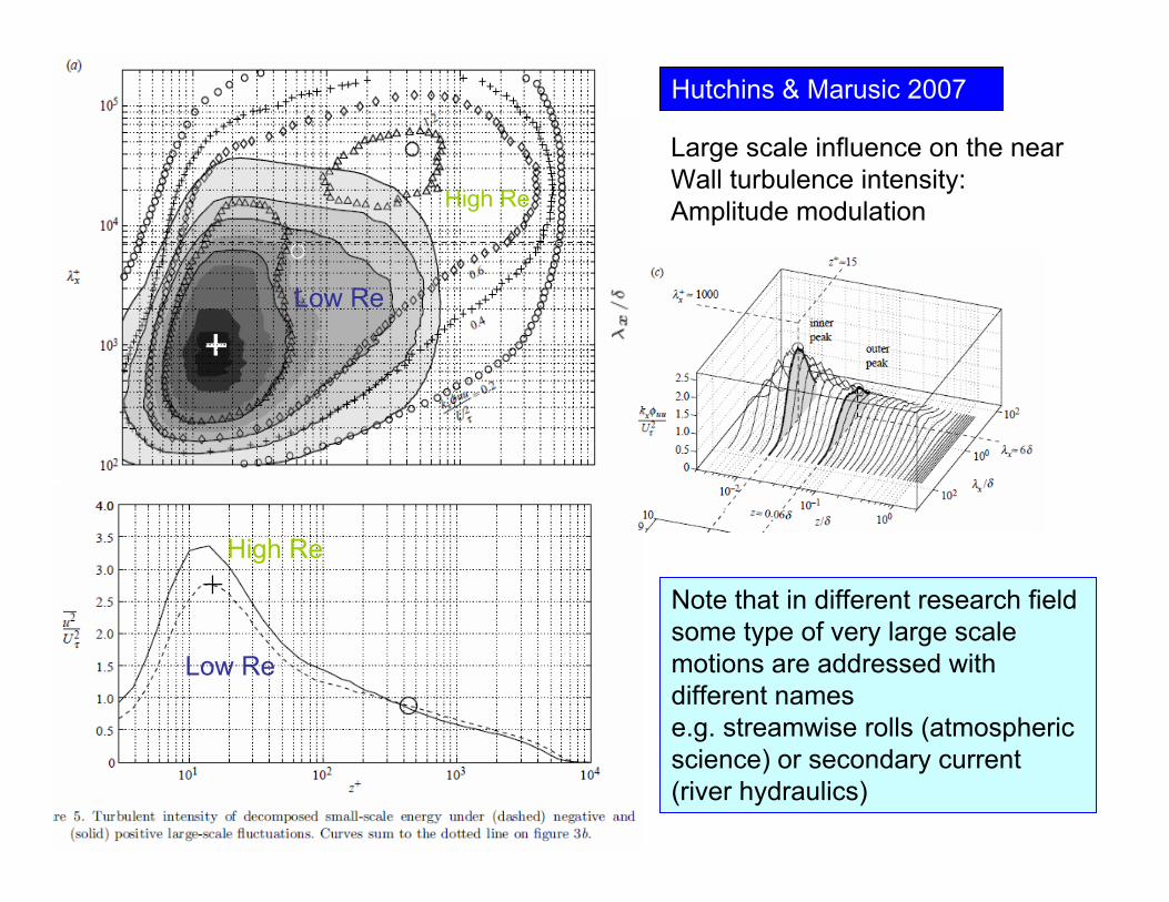
Hutchins & Marusic 2007

Large scale influence on the near Wall turbulence intensity: Amplitude modulation

Note that in different research fieldsome type of very large scale motions are addressed with different namese.g. streamwise rolls (atmospheric science) or secondary current (river hydraulics)

Low Re

High Re

High Re

Low Re

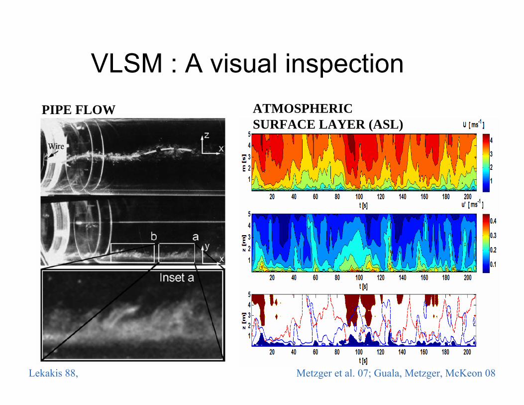
VLSM : A visual inspection

Lekakis 88, Metzger et al. 07; Guala, Metzger, McKeon 08

PIPE FLOW ATMOSPHERIC SURFACE LAYER (ASL)

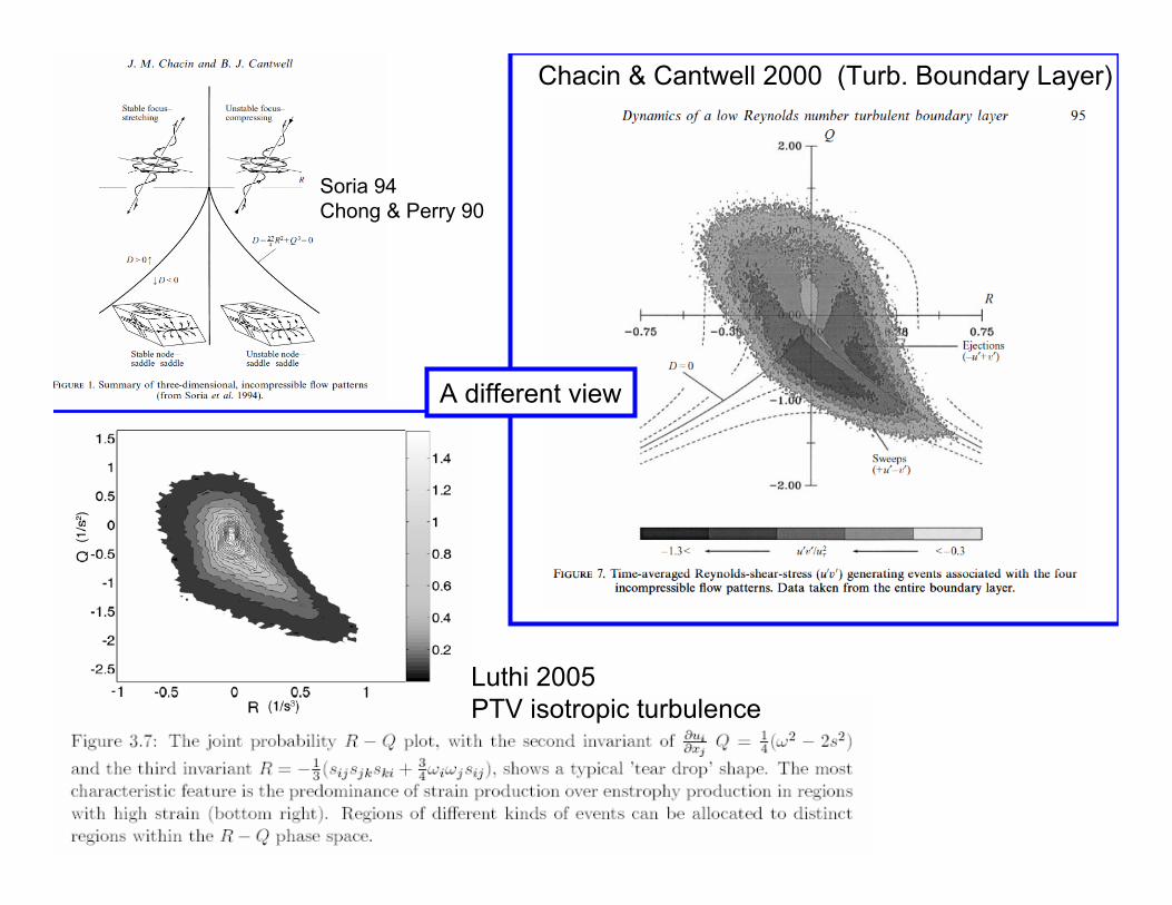
Chacin & Cantwell 2000 (Turb. Boundary Layer)

Soria 94Chong & Perry 90

Luthi 2005PTV isotropic turbulence

A different view

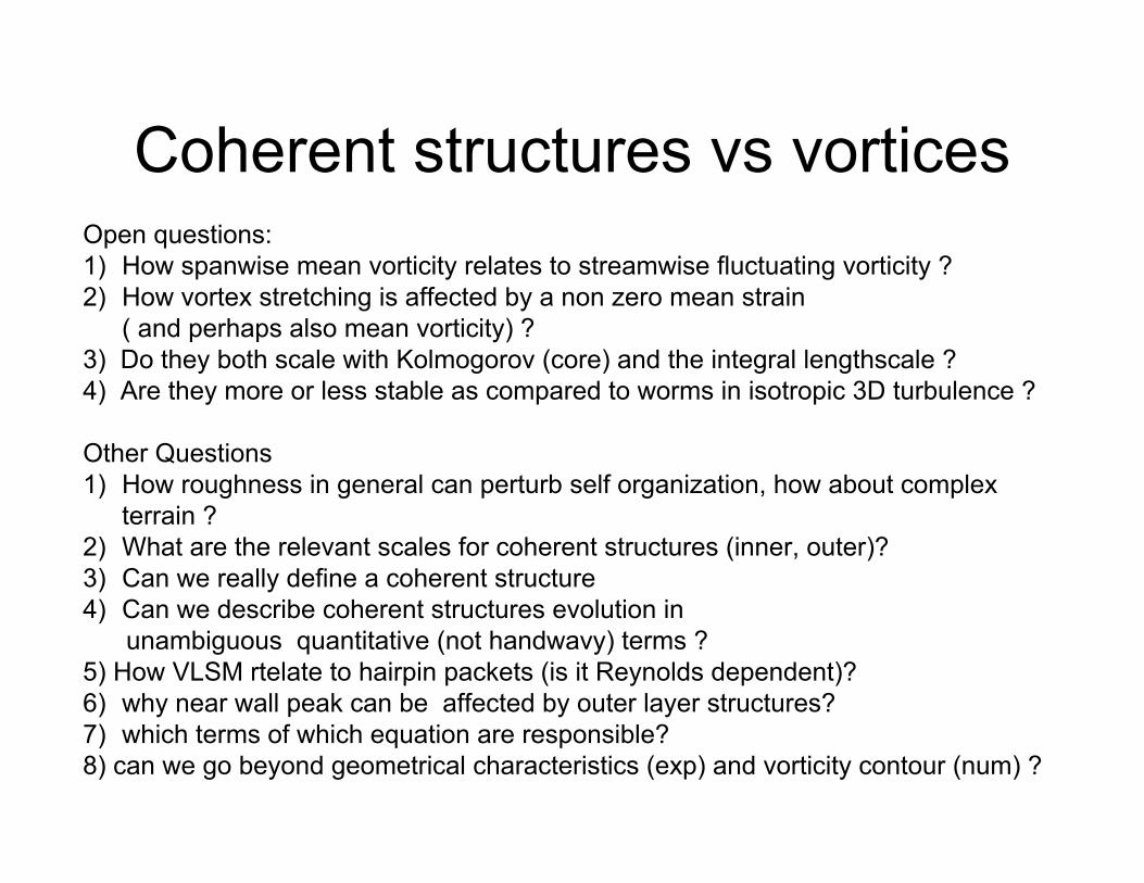
Coherent structures vs vorticesOpen questions: 1) How spanwise mean vorticity relates to streamwise fluctuating vorticity ?2) How vortex stretching is affected by a non zero mean strain

( and perhaps also mean vorticity) ?3) Do they both scale with Kolmogorov (core) and the integral lengthscale ?4) Are they more or less stable as compared to worms in isotropic 3D turbulence ?

Other Questions1) How roughness in general can perturb self organization, how about complex

terrain ?2) What are the relevant scales for coherent structures (inner, outer)?3) Can we really define a coherent structure 4) Can we describe coherent structures evolution in

unambiguous quantitative (not handwavy) terms ? 5) How VLSM rtelate to hairpin packets (is it Reynolds dependent)?6) why near wall peak can be affected by outer layer structures? 7) which terms of which equation are responsible?8) can we go beyond geometrical characteristics (exp) and vorticity contour (num) ?