arX

iv:c

ond-

mat

/970

6220

v2 [

cond

-mat

.sof

t] 2

5 Se

p 19

98

ICTP-SISSA

Coherent oscillations between two weakly coupled Bose-Einstein

Condensates: Josephson effects, π-oscillations, and macroscopic

quantum self trapping

S. Raghavan1, A. Smerzi2, S. Fantoni1,2, and S. R. Shenoy1

1) International Centre for Theoretical Physics, I-34100, Trieste, Italy

2) Istituto Nazionale de Fisica della Materia and International School for Advanced Studies, via

Beirut 2/4, I-34014, Trieste, Italy

(February 1, 2008)

Abstract

We discuss the coherent atomic oscillations between two weakly coupled

Bose-Einstein condensates. The weak link is provided by a laser barrier in a

(possibly asymmetric) double-well trap or by Raman coupling between two

condensates in different hyperfine levels. The Boson Josephson Junction

(BJJ) dynamics is described by the two-mode non-linear Gross-Pitaevskii

equation, that is solved analytically in terms of elliptic functions. The BJJ,

being a neutral, isolated system, allows the investigations of new dynamical

regimes for the phase difference across the junction and for the population

imbalance, that are not accessible with Superconductor Josephson Junctions

(SJJ). These include oscillations with either, or both of the following prop-

erties: 1) the time-averaged value of the phase is equal to π (π − phase

oscillations); 2) the average population imbalance is nonzero, in states with

“macroscopic quantum self-trapping” (MQST). The (non-sinusoidal) gener-

1

alization of the SJJ ‘ac’ and ‘plasma’ oscillations and the Shapiro resonance

can also be observed. We predict the collapse of experimental data (corre-

sponding to different trap geometries and total number of condensate atoms)

onto a single universal curve, for the inverse period of oscillations.

Analogies with Josephson oscillations between two weakly coupled reser-

voirs of 3He-B and the internal Josephson effect in 3He-A are also discussed.

PACS: 03.75.Fi,74.50.+r,05.30.Jp,32.80.Pj

Typeset using REVTEX

2

I. INTRODUCTION

Bose-Einstein condensation, predicted more than 70 years ago [1], was detected in 1995,

in a weakly interacting gas of alkali atoms held in magnetic traps [2]. Following the first

observations, there have been important experimental developments. A superposition of

condensate atoms in different hyperfine levels [3,4] has been created; non-destructive, in situ,

detection probes have tracked the dynamical evolution of a single condensate [5]. Further, the

evolution of the relative phase of two condensates has been measured through interferometry

techniques [6]. More recently, experiments that tune the scattering length by several orders

of magnitude [7] have opened the definite possibility of creating in the laboratory an ideal

condensate of non-interacting atoms.

The precise manipulation of this form of matter is of considerable theoretical interest:

besides the study of fundamental aspects of superfluidity from “first principles”, it is possible

to address “foundational” problems of quantum mechanics [8]. In fact, the order parame-

ter can be identified with the one-body macroscopic condensate wave function. This obeys

a nonlinear Schrodinger equation, known in the literature as the Gross-Pitaevskii equation

(GPE) [9]. The GPE has been successfully applied to study kinetic properties of the conden-

sate, like collective mode frequencies of trapped Bose-Einstein condensates (BEC) [10] and

the relaxation times of monopolar oscillations [11]. Chaotic behavior in dynamical quantum

observables [11,12], and the metastability of quantized vortices has been predicted [13].

The existence of spatial quantum coherence was demonstrated by cutting a single trapped

condensate by a far off-resonant laser sheet. Upon switch-off of the confining trap and the

laser, the two condensates overlapped, producing interference fringes [14], in analogy with

the a double-slit experiment with single electrons.

However, the superfluid nature of BEC can be fully tested only trough the existence of

superflows. Current experimental efforts are being focused on the creation of a Josephson

junction between two condensate bulks [14,15]. In this context, the Josephson junction

problem has been studied theoretically in the limit of non-interacting atoms [16], for small

3

amplitude Josephson oscillations [17,18], including finite temperature (damping) effects [18].

Furthermore, in connection with the quantum measurement problem, decoherence effects

and quantum corrections to the semiclassical mean-field dynamics [19,20] have also been

studied. Self trapping dynamics in the limit of small number of condensate atoms has been

considered [19] in the “quantum” and in the “semiclassical” (mean-field) approximation.

We have elsewhere, [21], pointed out that even though the Boson Josephson Junction (BJJ)

is a neutral-atom system, it can still display the (non-sinusoidal generalization of) typical

‘dc’, ‘ac’ and Shapiro effects occuring in charged Cooper-pair superconducting junctions.

Moreover, novel dynamical regimes like macroscopic quantum self trapping (for arbitrarily

large condensates) and π-phase oscillations (where the average value of the phase across the

junction is equal to π), have been predicted. In the present paper we present a comprehensive

analysis of the effects described in [21], including a discussion of the BJJ equations and

their analytic solution, and limits of the approximations underlying the BJJ model, and a

comparison with other superconducting and superfluid Josephson junctions.

The description of the GPE dynamics for a Bose condensate in a double-well trap re-

duces, under certain conditions, to a nonlinear, two-mode equation for the time-dependent

amplitudes ψ1,2(t) =√

N1,2(t)eiθ1,2(t), where N1,2(t) and θ1,2(t) are the number of atoms and

the phases of the condensate in the trap 1, 2 respectively. These amplitudes are coupled

by a tunneling matrix element between the two traps, with the spatial dependence of the

GPE wave function integrated out into constant parameters. The resulting BJJ tunneling

equations resemble the (nonlinear generalizations of) Superconductor Josephson Junction

(SJJ) equations, with the variables being the relative phase and the fractional population

imbalance.

However, there are important physical differences between the isolated double-well BJJ

and the SJJ with an external circuit. The SJJ is generally discussed in terms of a rigid

pendulum analogy in the resistively shunted junction (RSJ) model, while the BJJ in a double-

well trap can only be completely understood in terms of a non-rigid pendulum analogy,

with a length dependent on the angular momentum. In SJJ the Cooper-pair population

4

imbalance is identically zero (considering two equal-volume superconducting grains) due to

the presence of the external circuit [22], and the dynamical variable is the voltage ∼ φ across

a quasiparticle resistive shunt. In the BJJ, the non-rigid pendulum dynamics are associated

with superfluid density oscillations, of an isolated system. An isolated (without external

circuit) superconducting junction allows coherent Cooper-pair oscillations, but only in the

small amplitude (plasma) limit [22–24].

A closer analog of the BJJ is provided by the internal Josephson effect in 3He-A, where

the (rigid) pendulum oscillations describe the rate of change of up and down spin-pair

populations, induced by an external variable magnetic field [25–27]. The “π oscillations”

between two weakly coupled reservoirs of 3He-B [28] could be related to the analogous

oscillations occuring in BJJ.

The experimental detection of predicted effects in BJJ could be achieved through tempo-

ral modulations of phase-contrast fringes [14], interferometric techniques [6], or other probes

of atomic populations [29], using ∼ millisecond temporal oscillations of the integrated sig-

nal N1 − N2. The direct detection of the currents instead of densities, perhaps by Doppler

interferometry, would be worth exploring.

The plan of the paper is as follows: In Section II, we obtain the BJJ tunneling equations,

that, in Section III, are compared with the Josephson equation for other superconductor

and superfluid systems. In Section IV we solve the BJJ equations discussing the various

dynamical regimes. In Appendix A we outline the derivation of the two-mode BJJ from

GPE and discuss the limit of the approximations. The BJJ equations are solved analytically

in terms of elliptical functions in Appendix B. In the remainder of the paper Section V, we

discuss the asymmetric trap case, clarifying the analogies with the ac and Shapiro effect.

We summarize our results in Section VI.

5

II. BOSON JOSEPHSON JUNCTION: THE NON-LINEAR TWO-MODE

APPROXIMATION

The wavefunction Ψ(r, t) for an interacting BEC in a trap potential Vtrap(r, t) at T = 0

satisfies the GPE:

ih∂Ψ(r, t)

∂t= − h2

2m∇2Ψ(r, t) + [Vtrap(r) + g0|Ψ(r, t)|2]Ψ(r, t), (2.1)

with g0 = 4πh2a/m, m the atomic mass, and a the s-wave scattering length of the atoms

[30]. In the following we will consider a double-well trap produced, for example, by a far

off-resonant laser barrier that cuts a single trapped condensate into two (possibly asymmet-

ric) parts [14]. However, the results could also apply to the oscillations of the condensate

population difference between two hyperfine levels [15].

Since we are interested in the dynamical oscillations of the two weakly linked BEC, we

write a (time-dependent) variational wave-function as:

Ψ(r, t) = ψ1(t)Φ1(r) + ψ2(t)Φ2(r) (2.2)

with ψ1,2(t) =√

N1,2eiθ1,2(t) and a constant total number of atoms N1 +N2 = |ψ1|2 + |ψ2|2 =

NT . The amplitudes for general occupations N1,2(t), and phases θ1,2(t) obey the nonlinear

two-mode dynamical equations [18–21,31,32],

ih∂ψ1

∂t= (E0

1 + U1N1)ψ1 −Kψ2 (2.3a)

ih∂ψ2

∂t= (E0

2 + U2N2)ψ2 −Kψ1, (2.3b)

where damping and finite temperature effects are ignored. Here E01,2 are the zero-point en-

ergies in each well, U1,2N1,2 are proportional to the atomic self-interaction energies, and K

describes the amplitude of the tunneling between condensates, see Fig. 1. The constant pa-

rameters E01,2, U1,2,K can be written in terms of Φ1,2(r) wave-function overlaps. The Φ1,2(r),

roughly describing the condensate in each trap, can be expressed in terms of stationary

symmetric and antisymmetric eigenstates of GPE, (see Appendix A).

6

The fractional population imbalance

z(t) ≡ (N1(t) −N2(t))/NT ≡ (|ψ1|2 − |ψ2|2)/NT (2.4)

and relative phase

φ(t) ≡ θ2(t) − θ1(t) (2.5)

obey

z(t) = −√

1 − z2(t) sin(φ(t)), (2.6a)

φ(t) = ∆E + Λz(t) +z(t)

√

1 − z2(t)cos(φ(t)), (2.6b)

where we have rescaled to a dimensionless time, t2K/h→ t, and

∆E ≡ (E01 − E0

2)/2K + (U1 − U2)/2K, (2.7a)

Λ ≡ UNT /2K ; U ≡ (U1 + U2)/2 (2.7b)

The dimensionless parameters Λ and ∆E determine the dynamic regimes of the BEC atomic

tunneling. The total, conserved energy is:

H =Λz2

2+ ∆Ez −

√1 − z2 cosφ. (2.8)

suggesting that the equations of motion (2.6) can be written in the Hamiltonian form

z = −∂H∂φ

; φ =∂H

∂z, (2.9)

with z and φ, the canonically conjugate variables.

For well defined mean values in relativ population and phase, fluctuations must be small.

III. THE JOSEPHSON EFFECT IN OTHER SUPERFLUID AND

SUPERCONDUCTING SYSTEMS

The superconducting Josephson Junction (SJJ). We now consider the SJJ dy-

namic equations [22–24,33], for comparison with the BJJ tunneling equations of Eq. (2.6).

7

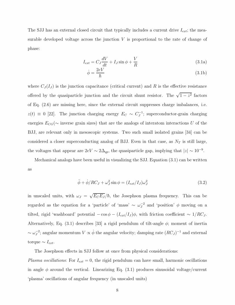
The SJJ has an external closed circuit that typically includes a current drive Iext; the mea-

surable developed voltage across the junction V is proportional to the rate of change of

phase:

Iext = CJdV

dt+ IJ sin φ+

V

R(3.1a)

φ =2eV

h(3.1b)

where CJ(IJ) is the junction capacitance (critical current) and R is the effective resistance

offered by the quasiparticle junction and the circuit shunt resistor. The√

1 − z2 factors

of Eq. (2.6) are missing here, since the external circuit suppresses charge imbalances, i.e.

z(t) ≡ 0 [22]. The junction charging energy EC ∼ C−1J ; superconductor-grain charging

energies ECG(∼ inverse grain sizes) that are the analogs of interatom interactions U of the

BJJ, are relevant only in mesoscopic systems. Two such small isolated grains [34] can be

considered a closer superconducting analog of BJJ. Even in that case, as NT is still large,

the voltages that appear are 2eV ∼ 2∆qp, the quasiparticle gap, implying that |z| ∼ 10−9.

Mechanical analogs have been useful in visualizing the SJJ. Equation (3.1) can be written

as

φ+ φ/RCJ + ω2J sin φ = (Iext/IJ)ω2

J (3.2)

in unscaled units, with ωJ =√ECEJ/h, the Josephson plasma frequency. This can be

regarded as the equation for a ‘particle’ of ‘mass’ ∼ ω−2J and ‘position’ φ moving on a

tilted, rigid ‘washboard’ potential − cosφ − (Iext/IJ)φ, with friction coefficient ∼ 1/RCJ .

Alternatively, Eq. (3.1) describes [33] a rigid pendulum of tilt-angle φ; moment of inertia

∼ ω−2J ; angular momentum V ∝ φ the angular velocity; damping rate (RCJ)−1 and external

torque ∼ Iext.

The Josephson effects in SJJ follow at once from physical considerations:

Plasma oscillations: For Iext = 0, the rigid pendulum can have small, harmonic oscillations

in angle φ around the vertical. Linearizing Eq. (3.1) produces sinusoidal voltage/current

‘plasma’ oscillations of angular frequency (in unscaled units)

8

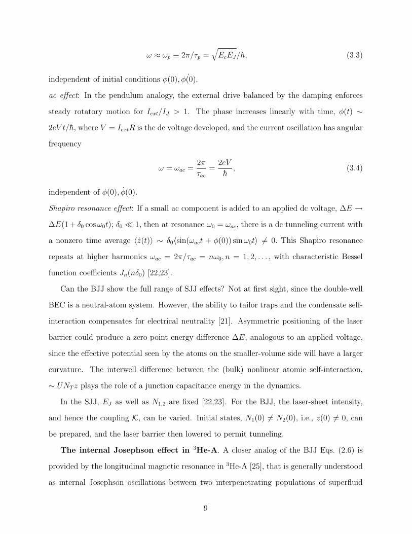
ω ≈ ωp ≡ 2π/τp =√

EcEJ/h, (3.3)

independent of initial conditions φ(0), ˙φ(0).

ac effect: In the pendulum analogy, the external drive balanced by the damping enforces

steady rotatory motion for Iext/IJ > 1. The phase increases linearly with time, φ(t) ∼

2eV t/h, where V = IextR is the dc voltage developed, and the current oscillation has angular

frequency

ω = ωac =2π

τac=

2eV

h, (3.4)

independent of φ(0), φ(0).

Shapiro resonance effect: If a small ac component is added to an applied dc voltage, ∆E →

∆E(1 + δ0 cosω0t); δ0 ≪ 1, then at resonance ω0 = ωac, there is a dc tunneling current with

a nonzero time average 〈z(t)〉 ∼ δ0〈sin(ωact + φ(0)) sinω0t〉 6= 0. This Shapiro resonance

repeats at higher harmonics ωac = 2π/τac = nω0, n = 1, 2, . . . , with characteristic Bessel

function coefficients Jn(nδ0) [22,23].

Can the BJJ show the full range of SJJ effects? Not at first sight, since the double-well

BEC is a neutral-atom system. However, the ability to tailor traps and the condensate self-

interaction compensates for electrical neutrality [21]. Asymmetric positioning of the laser

barrier could produce a zero-point energy difference ∆E, analogous to an applied voltage,

since the effective potential seen by the atoms on the smaller-volume side will have a larger

curvature. The interwell difference between the (bulk) nonlinear atomic self-interaction,

∼ UNT z plays the role of a junction capacitance energy in the dynamics.

In the SJJ, EJ as well as N1,2 are fixed [22,23]. For the BJJ, the laser-sheet intensity,

and hence the coupling K, can be varied. Initial states, N1(0) 6= N2(0), i.e., z(0) 6= 0, can

be prepared, and the laser barrier then lowered to permit tunneling.

The internal Josephson effect in 3He-A. A closer analog of the BJJ Eqs. (2.6) is

provided by the longitudinal magnetic resonance in 3He-A [25], that is generally understood

as internal Josephson oscillations between two interpenetrating populations of superfluid

9

up-down spin-pairs [26]. The weak coupling is provided by the dipole interaction between

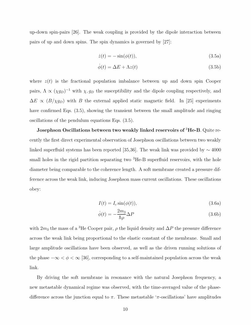
pairs of up and down spins. The spin dynamics is governed by [27]:

z(t) = − sin(φ(t)), (3.5a)

φ(t) = ∆E + Λz(t) (3.5b)

where z(t) is the fractional population imbalance between up and down spin Cooper

pairs, Λ ∝ (χgD)−1 with χ, gD the susceptibility and the dipole coupling respectively, and

∆E ∝ (B/χgD) with B the external applied static magnetic field. In [25] experiments

have confirmed Eqs. (3.5), showing the transient between the small amplitude and ringing

oscillations of the pendulum equations Eqs. (3.5).

Josephson Oscillations between two weakly linked reservoirs of 3He-B. Quite re-

cently the first direct experimental observation of Josephson oscillations between two weakly

linked superfluid systems has been reported [35,36]. The weak link was provided by ∼ 4000

small holes in the rigid partition separating two 3He-B superfluid reservoirs, with the hole

diameter being comparable to the coherence length. A soft membrane created a pressure dif-

ference across the weak link, inducing Josephson mass current oscillations. These oscillations

obey:

I(t) = Ic sin(φ(t)), (3.6a)

φ(t) = −2m3

hρ∆P (3.6b)

with 2m3 the mass of a 3He Cooper pair, ρ the liquid density and ∆P the pressure difference

across the weak link being proportional to the elastic constant of the membrane. Small and

large amplitude oscillations have been observed, as well as the driven running solutions of

the phase −∞ < φ <∞ [36], corresponding to a self-maintained population across the weak

link.

By driving the soft membrane in resonance with the natural Josephson frequency, a

new metastable dynamical regime was observed, with the time-averaged value of the phase-

difference across the junction equal to π. These metastable ‘π-oscillations’ have amplitudes

10

and frequencies smaller than the ‘stable’ Josephson oscillations, into which they decay with

a life time that increases with decreasing temperature [28]. Analogous π-oscillations with

similar properties are described by BJJ (see Section IV). In a different context, π-junctions

have been created with high-Tc superconductors, that reflect the symmetry of the d-wave

pairing state [37].

IV. THE SYMMETRIC TRAP CASE, ∆E = 0

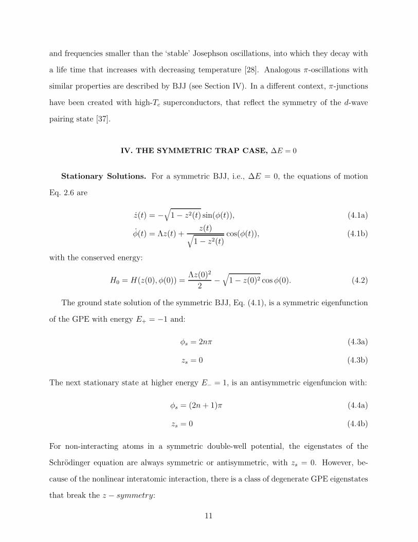
Stationary Solutions. For a symmetric BJJ, i.e., ∆E = 0, the equations of motion

Eq. 2.6 are

z(t) = −√

1 − z2(t) sin(φ(t)), (4.1a)

φ(t) = Λz(t) +z(t)

√

1 − z2(t)cos(φ(t)), (4.1b)

with the conserved energy:

H0 = H(z(0), φ(0)) =Λz(0)2

2−√

1 − z(0)2 cosφ(0). (4.2)

The ground state solution of the symmetric BJJ, Eq. (4.1), is a symmetric eigenfunction

of the GPE with energy E+ = −1 and:

φs = 2nπ (4.3a)

zs = 0 (4.3b)

The next stationary state at higher energy E− = 1, is an antisymmetric eigenfuncion with:

φs = (2n+ 1)π (4.4a)

zs = 0 (4.4b)

For non-interacting atoms in a symmetric double-well potential, the eigenstates of the

Schrodinger equation are always symmetric or antisymmetric, with zs = 0. However, be-

cause of the nonlinear interatomic interaction, there is a class of degenerate GPE eigenstates

that break the z − symmetry:

11

φs = (2n+ 1)π (4.5a)

zs = ±√

1 − 1

Λ2(4.5b)

provided that |Λ| > 1. The energy for this state is Esb = 12

(

Λ + 1Λ

)

.

These z-symmetry breaking states are an artifact of the semiclassical limit in which the

GPE has been derived. In a full quantum two mode approximation the eigenstates are

always symmetric in the population imbalance: as we will discuss later, such states have a

large lifetime that scales exponentially with the total number of atoms.

Rabi Oscillations. For noninteracting atoms (Λ = 0) Eqs. (4.1) describe sinusoidal

Rabi oscillations between the two traps with frequency ωR = 2hK. These oscillations are

equivalent to single atom dynamics, rather than a Josephson-effect arising from the inter-

acting superfluid condensate. The possibility to tune the scattering length to values very

close to zero [7], open avenues for their experimental observation.

Zero-phase modes. These modes describe the intra-well atomic tunneling dynamics

with a zero time-average value of the phase across the junction, 〈φ(t)〉 = 0, and 〈z〉 = 0. To

this dynamical class belong small and large amplitude condensate oscillations.

Small amplitude oscillations. The small amplitude, or “plasma” (in analogy with SJJ),

effect follows at once from the pendulum analogy. From Eq. (4.1), the BJJ is like a non-rigid

pendulum of length

(x2 + y2)1/2 =√

1 − z2 (4.6)

decreasing with angular momentum z, and with moment of inertia Λ−1. Linearizing

Eq. (4.1), we obtain sinusoidal oscillations with inverse periods (in unscaled units)

τ−1L =

√

2UNTK + (2K)2/2πh, (4.7)

independent of the initial conditions z(0), φ(0). The comparison between Eq. (4.7) and

Eq. (3.3) indicates that 2NTK (∼ NT ) is the analog of the Josephson coupling energy EJ ,

while U (∼ N−d/5T , with d the dimensionality of the system) is the analog of the capacitive

12

energy EC . Since the coupling energy, fixed by the laser profile, is K ∼ A, the tunnel junction

area whereas the bulk interaction, UNT , is independent of A, the oscillation rate goes as

τ−1L ∼ A1/2. (The plasma frequency for SJJ, τ−1

p ∼√EcEJ by contrast, is independent of

A, as EJ ∼ A,Ec ∼ A−1).

The Josephson-like length ‘λJ ’ ≡√

h2/2mK, that governs spatial variation along the

junction, should be much greater than ∼√A to justify neglect of spatial variations of z, φ,

i.e., to obtain a ‘flat plasmon’ spectrum. For K = 0.1nK, one finds ‘λJ ’ ∼ 10µm. We will

not, however, consider such spatial variations here. The frequency of the small amplitude

oscillations in BJJ are of the order of 10 − 100 Hz for typical trap parameters, and should

be compared with the frequencies of plasma SJJ that are of the order of GHz.

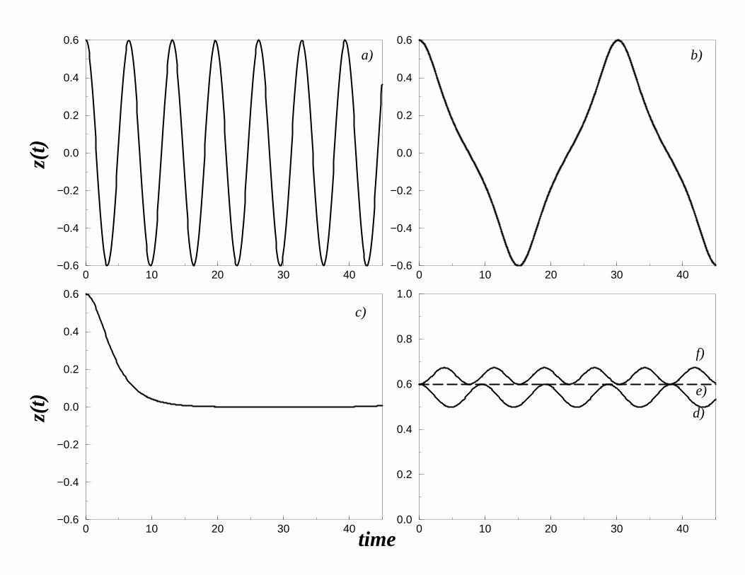
Large amplitude oscillations. In Fig. 2 we display this regime of anharmonic oscillations,

plotting z = N1−N2

NTas a function of time, with the initial value of the phase difference

φ(0) = 0 and Λ = 10, and for increasing values of the inital population imbalance z(0).

Specifically, z(0) takes on the values 0.1, 0.5, 0.59, 0.6, and 0.65 from a) through e) respec-

tively. Increasing z(0) for fixed Λ, (or increasing Λ for fixed z(0)) adds higher harmonics to

the sinusoidal oscillations, corresponding to large amplitude oscillations of the (non-rigid)

pendulum. This is shown in Fig. 2 (b,c). The period of such oscillations increases with z(0),

then decreases, undergoing a critical slowing down (Fig. 2(d), dashed line), with a logarith-

mic divergence. The singularity in the period corresponds to the pendulum in a vertically

upright position, i.e., reaching the fixed point of Eq. (4.4b).

Running-phase modes: Macroscopic Quantum Self-Trapping. In addition to

anharmonic and critically slow oscillations, other striking effects occurin BJJ. For instance,

for a fixed value of the initial population imbalance, if the self-interaction parameter Λ

exceeds a critical value Λc, the populations become macroscopically self-trapped with 〈z〉 6=

0. There are different ways in which this state can be achieved and all of them correspond

to the condition (which we shall term the MQST condition) that

H0 ≡ H(z(0), φ(0)) =Λ

2z(0)2 −

√

1 − z(0)2 cos(φ(0)) > 1 (4.8)

13

In a series of experiments in which φ(0) and z(0) are kept constant but Λ is varied (by

changing the geometry or the total number of condensate atoms, for example), the critical

parameter for MQST is

Λc =1 +

√

1 − z(0)2 cos(φ(0))

z(0)2/2. (4.9)

On the other hand, changing the initial value of the population imbalance z(0) with a fixed

trap geometry and total number of condensate atoms (and initial value φ(0)), Λ remains

constant and Eq. (4.8) defines a critical population imbalance zc. As we shall see in this and

the next section, for φ(0) = 0, if z(0) > zc, MQST sets in, but for φ(0) = π, z(0) < zc marks

the region of MQST. More generally, if |φ(0)| ≤ π/2, MQST occurs for z(0) > zc while for

other values of φ(0), it occurs for z(0) < zc.

In this section, we will discuss the type of MQST in which the phase difference of the

order parameter across the BJJ runs without bound; other types are discussed later. The

phenomenon can be understood through the pendulum analogy. If the population imbalances

are prepared such that the initial ‘angular kinetic energy’ of the pendulum, z2(0), exceeds the

potential energy barrier height of the vertically displaced φ = π ‘pendulum orientation’, there

will occur a steady self-sustained ‘pendulum rotation’, with nonzero angular momentum 〈z〉,

and a closed-loop trajectory around the pendulum support. For H0 < 1 the population

imbalance oscillates about a zero value. For H0 > 1 the time-averaged ‘angular momentum’

is nonzero, 〈z(t)〉 6= 0, with oscillations around this nonzero value (Fig. 2). MQST is a

nonlinear effect arising from the self-interaction ∼ UNT z2 of the atoms. It is dependent on

the trap parameters, total number of atoms, and initial conditions, and is self-maintained

in a closed conservative system without external drives. Although the SJJ ‘ac’ effect in the

RCSJ model involves a running-phase, it is clearly physically different from MQST, as it is

a driven steady-state independent of initial conditions. Moreover, in SJJ the Cooper pair

population imbalance are locked to zero by the external circuit. MQST differs from single-

electron Coulomb blockade effect that involves a single electron. It also differs from the

self-trapping of polarons [32] that arise from single electrons interacting with a polarizable

14

lattice: arising, instead, from self-interaction of a macroscopically large, number of coherent

atoms.

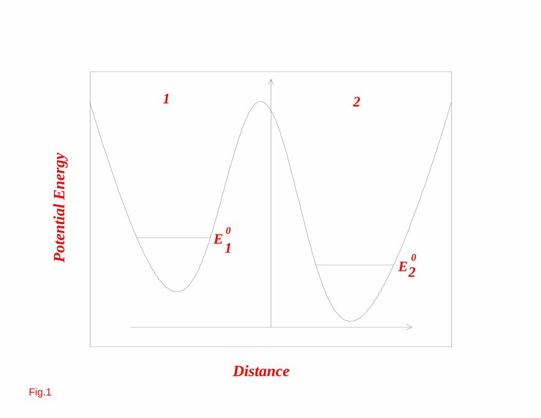
π-phase modes These modes describe the tunneling dynamics in which the time-

averaged value of the phase across the junction is 〈φ〉 = π.

The modes arise once more from the non-rigidity (momentum dependent length) of the

pendulum and are not observable with SJJ. Thei include small amplitude, large amplitude,

and macroscopic self-trapped oscillations. The last has nonzero average population imbalanc,

while < z >= 0 for the others. We summarize this behavior in the temporal evolution of

z(t) in Fig. 3 for z(0) = 0.6, φ(0) = π. Λ takes the values 0.1, 1.1, 1.111, 1.2, 1.25, and 1.3

in Figs. 3(a-f) respectively.

Small amplitude oscillations. For small z, Eqs. (4.1) can be linearized around the fixed point

(4.4b) yielding harmonic oscillations for Λ < 1, with a period (in unscaled units):

τ−1π =

√

(2K)2 − 2UNTK/2πh. (4.10)

It is worth noticing that the ratio of the frequency of the small amplitude zero- and π- mode

phase oscillations is τL

τπ=√

1−Λ1+Λ

< 1 (similar to the 3He-B π-oscillations of Section III).

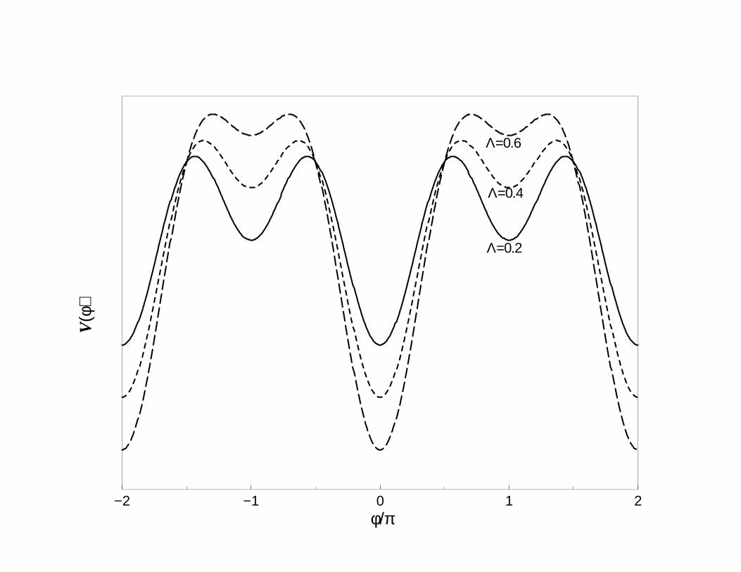
Linearizing Eqs. (4.1) in z only, the BJJ Eq. (4.1b) reduces to the very simple form:

φ = −[Λ sin(φ) +1

2sin(2φ)] +O(z2) (4.11)

This suggests a mechanical analogy in which a particle of spatial coordinate φ moves in

the potential:

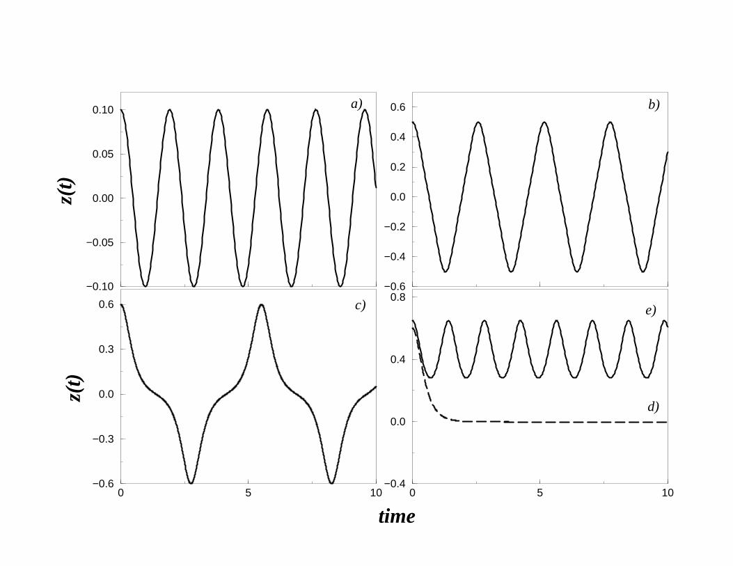
V (φ) = −Λ cos(φ) − 1

4cos(2φ) +O(z2) (4.12)

In Fig. 4 we see that V (φ) has a small valley around φ = π where the particle can oscillate.

The depth of this valley decreases as Λ → 1. The valley persists, in the full potential for

V (φ), retaining all the higher order terms in z.

Large amplitude oscillations For π-phase oscillations, the momentum dependent length

allows the pendulum bob to make inverted anharmonic oscillations with 〈z〉 = 0 around the

15

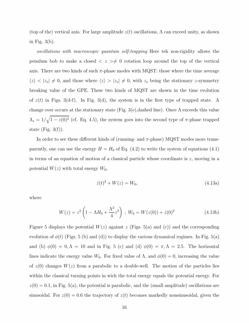
(top of the) vertical axis. For large amplitude z(t) oscillations, Λ can exceed unity, as shown

in Fig. 3(b).

oscillations with macroscopic quantum self-trapping Here teh non-rigidity allows the

penulum bob to make a closed < z > 6= 0 rotation loop around the top of the vertical

axis. There are two kinds of such π-phase modes with MQST: those where the time average

〈z〉 < |zs| 6= 0, and those where 〈z〉 > |zs| 6= 0, with zs being the stationary z-symmetry

breaking value of the GPE. These two kinds of MQST are shown in the time evolution

of z(t) in Figs. 3(d-f). In Fig. 3(d), the system is in the first type of trapped state. A

change over occurs at the stationary state (Fig. 3(e),dashed line). Once Λ exceeds this value

Λs = 1/√

1 − z(0)2 (cf. Eq. 4.5), the system goes into the second type of π-phase trapped

state (Fig. 3(f)).

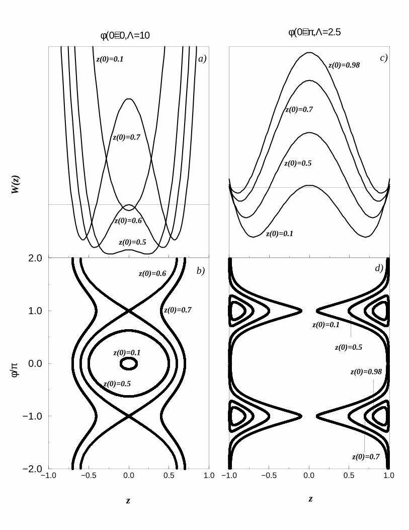
In order to see these different kinds of (running- and π-phase) MQST modes more trans-

parently, one can use the energy H = H0 of Eq. (4.2) to write the system of equations (4.1)

in terms of an equation of motion of a classical particle whose coordinate is z, moving in a

potential W (z) with total energy W0,

z(t)2 +W (z) = W0, (4.13a)

where

W (z) = z2

(

1 − ΛH0 +Λ2

4z2

)

; W0 = W (z(0)) + z(0)2 (4.13b)

Figure 5 displays the potential W (z) against z (Figs. 5(a) and (c)) and the corresponding

evolution of φ(t) (Figs. 5 (b) and (d)) to display the various dynamical regimes. In Fig. 5(a)

and (b) φ(0) = 0,Λ = 10 and in Fig. 5 (c) and (d) φ(0) = π,Λ = 2.5. The horizontal

lines indicate the energy value W0. For fixed value of Λ, and φ(0) = 0, increasing the value

of z(0) changes W (z) from a parabolic to a double-well. The motion of the particles lies

within the classical turning points in wich the total energy equals the potential energy. For

z(0) = 0.1, in Fig. 5(a), the potential is parabolic, and the (small amplitude) oscillations are

sinusoidal. For z(0) = 0.6 the trajectory of z(t) becomes markedly nonsinusoidal, given the

16

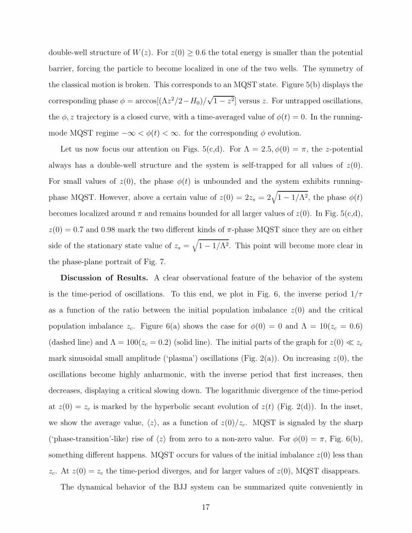
double-well structure of W (z). For z(0) ≥ 0.6 the total energy is smaller than the potential

barrier, forcing the particle to become localized in one of the two wells. The symmetry of

the classical motion is broken. This corresponds to an MQST state. Figure 5(b) displays the

corresponding phase φ = arccos[(Λz2/2−H0)/√

1 − z2] versus z. For untrapped oscillations,

the φ, z trajectory is a closed curve, with a time-averaged value of φ(t) = 0. In the running-

mode MQST regime −∞ < φ(t) <∞. for the corresponding φ evolution.

Let us now focus our attention on Figs. 5(c,d). For Λ = 2.5, φ(0) = π, the z-potential

always has a double-well structure and the system is self-trapped for all values of z(0).

For small values of z(0), the phase φ(t) is unbounded and the system exhibits running-

phase MQST. However, above a certain value of z(0) = 2zs = 2√

1 − 1/Λ2, the phase φ(t)

becomes localized around π and remains bounded for all larger values of z(0). In Fig. 5(c,d),

z(0) = 0.7 and 0.98 mark the two different kinds of π-phase MQST since they are on either

side of the stationary state value of zs =√

1 − 1/Λ2. This point will become more clear in

the phase-plane portrait of Fig. 7.

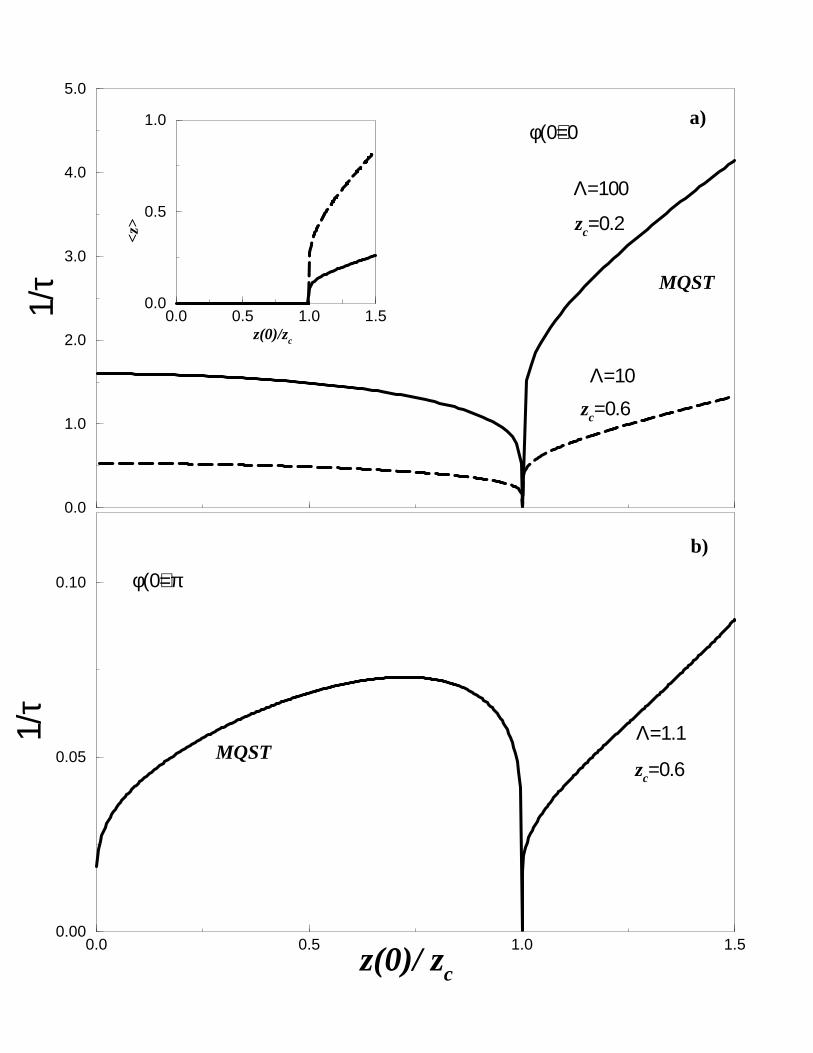
Discussion of Results. A clear observational feature of the behavior of the system

is the time-period of oscillations. To this end, we plot in Fig. 6, the inverse period 1/τ

as a function of the ratio between the initial population imbalance z(0) and the critical

population imbalance zc. Figure 6(a) shows the case for φ(0) = 0 and Λ = 10(zc = 0.6)

(dashed line) and Λ = 100(zc = 0.2) (solid line). The initial parts of the graph for z(0) ≪ zc

mark sinusoidal small amplitude (‘plasma’) oscillations (Fig. 2(a)). On increasing z(0), the

oscillations become highly anharmonic, with the inverse period that first increases, then

decreases, displaying a critical slowing down. The logarithmic divergence of the time-period

at z(0) = zc is marked by the hyperbolic secant evolution of z(t) (Fig. 2(d)). In the inset,

we show the average value, 〈z〉, as a function of z(0)/zc. MQST is signaled by the sharp

(‘phase-transition’-like) rise of 〈z〉 from zero to a non-zero value. For φ(0) = π, Fig. 6(b),

something different happens. MQST occurs for values of the initial imbalance z(0) less than

zc. At z(0) = zc the time-period diverges, and for larger values of z(0), MQST disappears.

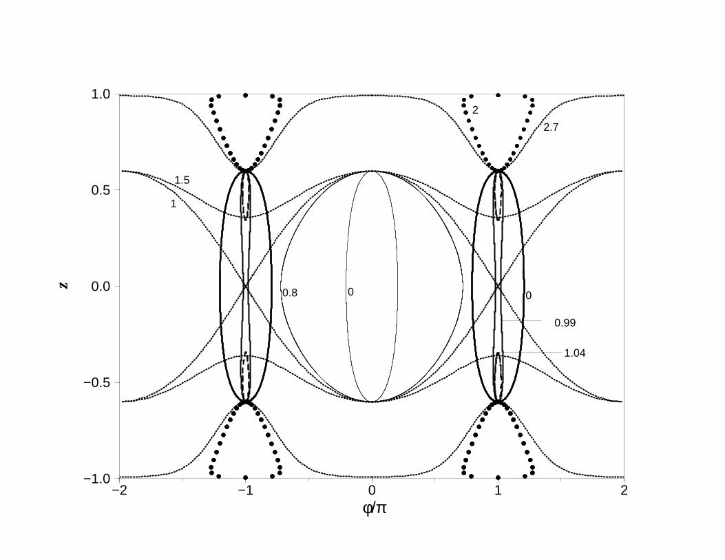
The dynamical behavior of the BJJ system can be summarized quite conveniently in

17

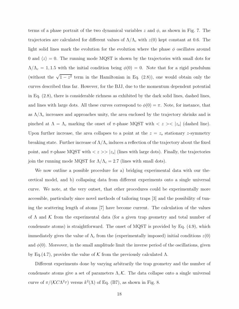
terms of a phase portrait of the two dynamical variables z and φ, as shown in Fig. 7. The

trajectories are calculated for different values of Λ/Λc with z(0) kept constant at 0.6. The

light solid lines mark the evolution for the evolution where the phase φ oscillates around

0 and 〈z〉 = 0. The running mode MQST is shown by the trajectories with small dots for

Λ/Λc = 1, 1.5 with the initial condition being φ(0) = 0. Note that for a rigid pendulum

(without the√

1 − z2 term in the Hamiltonian in Eq. (2.8)), one would obtain only the

curves described thus far. However, for the BJJ, due to the momentum dependent potential

in Eq. (2.8), there is considerable richness as exhibited by the dark solid lines, dashed lines,

and lines with large dots. All these curves correspond to φ(0) = π. Note, for instance, that

as Λ/Λc increases and approaches unity, the area enclosed by the trajectory shrinks and is

pinched at Λ = Λc marking the onset of π-phase MQST with < z >< |zs| (dashed line).

Upon further increase, the area collapses to a point at the z = zs stationary z-symmetry

breaking state. Further increase of Λ/Λc induces a reflection of the trajectory about the fixed

point, and π-phase MQST with < z >> |zs| (lines with large dots). Finally, the trajectories

join the running mode MQST for Λ/Λc = 2.7 (lines with small dots).

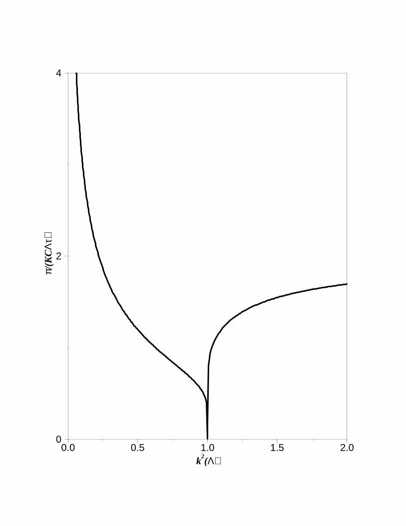
We now outline a possible procedure for a) bridging experimental data with our the-

oretical model, and b) collapsing data from different experiments onto a single universal

curve. We note, at the very outset, that other procedures could be experimentally more

accessible, particularly since novel methods of tailoring traps [3] and the possibility of tun-

ing the scattering length of atoms [7] have become current. The calculation of the values

of Λ and K from the experimental data (for a given trap geometry and total number of

condensate atoms) is straightforward. The onset of MQST is provided by Eq. (4.9), which

immediately gives the value of Λc from the (experimentally imposed) initial conditions z(0)

and φ(0). Moreover, in the small amplitude limit the inverse period of the oscillations, given

by Eq.(4.7), provides the value of K from the previously calculated Λ.

Different experiments done by varying arbitrarily the trap geometry and the number of

condensate atoms give a set of parameters Λ,K. The data collapse onto a single universal

curve of π/(KCΛ2τ) versus k2(Λ) of Eq. (B7), as shown in Fig. 8.

18

The parameters UNT , and E0 can be estimated to be ∼ 100nK and ∼ 10nK respectively

for NT = 104 if we take the trap-frequency ωtrap to be ∼ 100Hz. Λ = UNT /2K can be

varied widely by changing NT or the barrier height ∼ K that depends exponentially on

the laser-sheet thickness. Typical frequencies are then 1/τL ∼ 100Hz. With collective

mode excitation energies ∆coll ∼ E0, and quasiparticle gaps ∆qp ∼√UNTE0, for UNT z <

∆qp,coll intra-well excitations are not induced. At nonzero temperatures, BEC depletion and

thermal fluctuations will renormalize the parameters in Eq. (2.7), and will damp [18] the

coherent oscillations. The effects of damping on the oscillation behaviour requires a separete

treatment and will be considered elsewhere.

V. THE ASYMMETRIC TRAP CASE, ∆E 6= 0

Exact solutions and temporal behavior. Let us now consider the case where the

traps are asymmetric, i.e., ∆E 6= 0, as in Fig. 1, with Hamiltonian

H =Λz2

2+ ∆Ez −

√1 − z2 cosφ. (5.1)

For Λz(0) ≪ ∆E, the non-rigid pendulum is driven to rotate in a direction determined by

∆E (corresponding to the ac Josephson-like effect). With ∆E = 0, and Λ > Λc (of Eq. (4.9),

we had found that the pendulum also executes rotatory motion, in a direction determined

by z(0). For Λz(0) ≫ ∆E 6= 0, we expect this type of motion to persist (corresponding

to MQST due to nonlinearity). In between there should be competition between the two

effects, and a transition at some shifted critical value Λ = Λc(∆E). This physical picture

for ∆E 6= 0 is confirmed by obtaining z(t) in terms of Weierstrassian elliptic functions that

change their behavior at a singular value Λ = Λc(∆E).

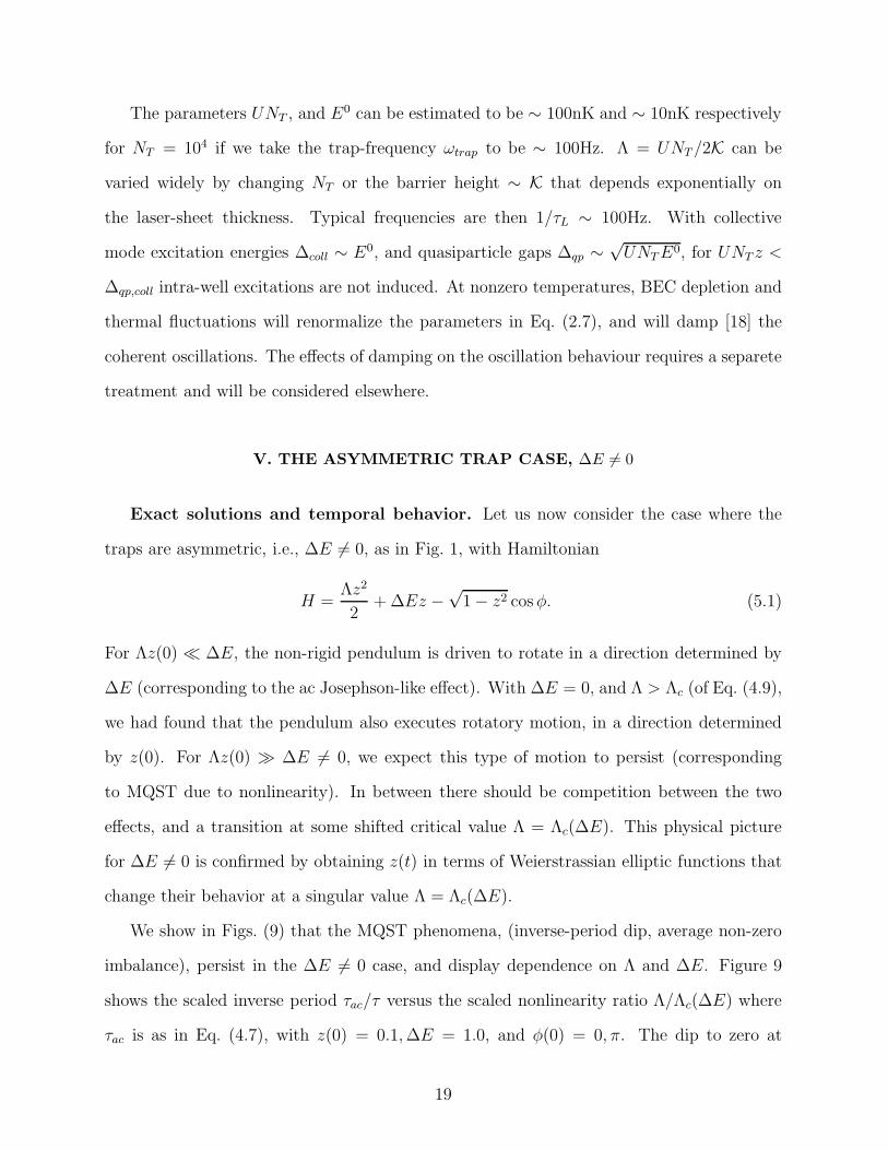
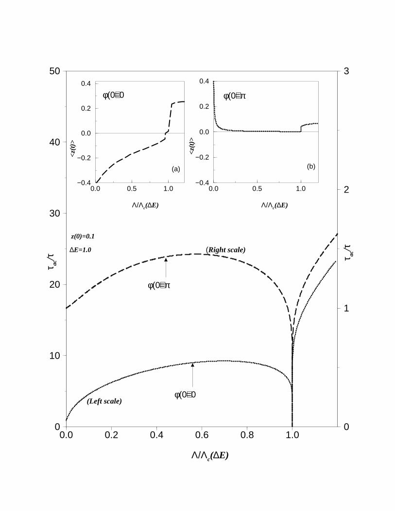
We show in Figs. (9) that the MQST phenomena, (inverse-period dip, average non-zero

imbalance), persist in the ∆E 6= 0 case, and display dependence on Λ and ∆E. Figure 9

shows the scaled inverse period τac/τ versus the scaled nonlinearity ratio Λ/Λc(∆E) where

τac is as in Eq. (4.7), with z(0) = 0.1,∆E = 1.0, and φ(0) = 0, π. The dip to zero at

19

the onset of MQST is clearly seen. The inset shows the time-averaged 〈z〉 for φ(0) = 0, π,

vanishing at Λ = Λc(∆E). Whereas for ∆E = 0 and Λ < Λc(∆E = 0), the average

population imbalance was zero, for ∆E 6= 0 we have 〈z〉 6= 0 in the corresponding sub-

critical region Λ < Λc(∆E). This is analogous to a voltage across a capacitor inducing

a charge difference and the external static magnetic field in the case of 3He-A Note that

there is a combined influence of Λ,∆E, φ(0), so 〈z〉 can be larger (in magnitude) than z(0).

In particular, for Λ → 0, 〈z〉 → −∆E(√

1 − z2(0) cos φ(0) − ∆Ez(0))/(1 + ∆E2), that for

φ(0) = 0 is negative, as in the inset. This corresponds to an averaged pendulum rotation

〈z〉 ∼ −∆E < 0, opposite in sign to the initial z(0) > 0, but slowing to zero as the critical

value is approached. For Λ > Λc(∆E), in the MQST regime, the averaged rotation 〈z〉 > 0

is in the initial direction of z(0) > 0, with 〈z〉 approaching the initial z(0) value for large Λ,

as in the ∆E = 0 case of Fig. 8.

Shapiro Effect Analogs. Let us now consider the BJJ analog of the Shapiro resonance

effect observed in SJJ [23]. In addition to a time-independent trap asymmetry ∆E, we

impose a sinusoidal variation so that we can write the asymmetry term as ∆E+∆E1 cosω0t.

This could be done by varying the laser barrier position at fixed intensity. A similar Shapiro-

like resonance effect could be seen, with an oscillation of the laser beam intensity, at fixed

mid-position, so K → K(1 + δ0 cosω0t). The analog of the Shapiro effect arises when the

period from the time independent asymmetry, ∼ 1/∆E, matches that from the oscillatory

increment, ∼ 1/ω0. This matching condition is intimately connected with the phenomenon of

Bloch oscillations and dynamic localization in crystals and trapping in two-level atoms [38].

The dc value of the drift current, 〈z(t)〉, as a function of ∆E, will show up as resonant spikes.

(For SJJ, with current drives, the Shapiro effect shows up as steps in the I-V characteristics.)

Of course, the dc drift cannot persist indefinitely, because the phase difference between the

condensates on the two parts of the BJJ will cease to be a well-defined quantity once the

population in one well drops below Nmin.

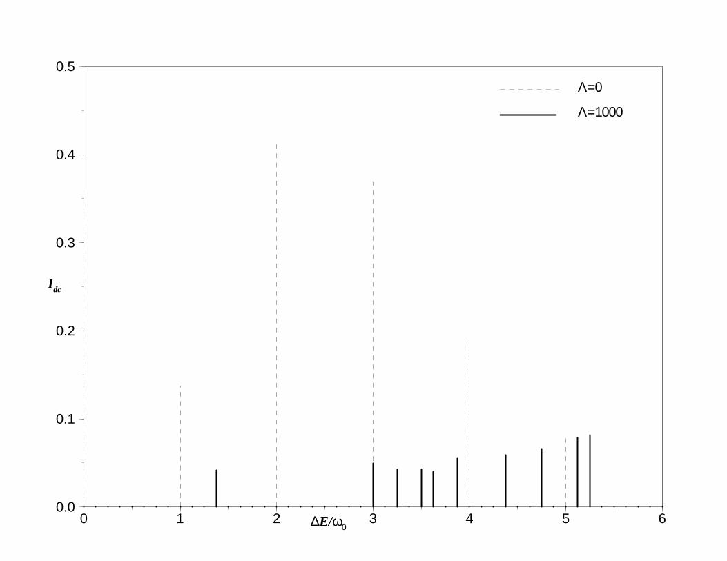
Figure 10 shows Idc ∝ 〈z(t)〉 obtained from time averaging the numerical solution, with

a small ac drive and ∆E 6= 0. It is plotted as a function of ∆E/ω0 for increasing values

20

of the nonlinearity ratio Λ. The initial conditions are z(0) ∼ 0 = 0.045, φ(0) = π/2, for

which Λc ∼ 1000 (in the absence of ∆E and ac driving). When Λ is zero, sharp peaks in

Idc occur at the usual ‘Shapiro’ condition values ∆E ∝ nω0, n = 1, 2, . . .. As Λ increases,

however, two things happen. Firstly, multiple peaks also occur at ∆E/ω0 values different

from integers. Close to the MQST regime, (Λ ∼ Λc), there is a proliferation of peaks as

the system moves from a regime of constant current, 〈z〉 6= 0 (Λ small), to one of constant

population imbalance 〈z〉 6= 0 (Λ large). Secondly, the magnitude of the peaks or dc currents

decreases.

Finally, we note that for ∆E larger than the Bogoliubov quasiparticle gap ∆qp, and high

enough temperatures, a dissipative quasiparticle branch might be observable.

VI. SUMMARY

We have investigated the Josephson dynamics in two weakly linked Bose-Einstein con-

densates forming a Boson Josephson junction. In the resulting nonlinear two-mode model,

we have described the temporal oscillations of the population imbalance of the conden-

sates in terms of elliptic functions. Our predictions include non-sinusoidal generalizations of

Josephson ‘dc’, ‘ac’ and Shapiro effects. We also predict macroscopic quantum self-trapping

which is a self-maintained population imbalance across the junction due to atomic self-

interaction, and π-oscillations, in which the phase difference across the junction oscillates

around π. We clarify the connection and the differences between these phenomena and oth-

ers occuring in related systems like the superconducting Josephson junctions, the internal

Josephson effect in 3He-A, and Josephson oscillations between two weakly linked reservoirs

of 3He-B. Through a set of functional relations, we also predict the collapse of experimental

data (corresponding to different trap geometries and total number of condensate atoms)

onto a single universal curve. These effects constitute experimentally testable signatures of

quantum phase coherence and the superfluid character of weakly interacting Bose-Einstein

condensates.

21

Discussions with V. Chandrasekhar, S. Giovanazzi, L. Glazman, A. J. Leggett, E. Tosatti

and useful references from G. Williams are acknowledged.

APPENDIX A: MICROSCOPIC DERIVATION OF THE BOSON JOSEPHSON

EQUATION FROM THE GROSS-PITAEVSKII EQUATION

The values of the constant parameters in BJJ Eqs. (2.3) K, E0, and U depend on the

geometry (and effective dimensionality) of the system and the total number of condensate

atoms. We now outline their dependence in term of spatial GPE wave functions, elucidating

the approximations underlying the BJJ equations.

We look for the solution of the (time-dependent) GPE (2.1) with the following

variational ansatz:

Ψ(r, t) = ψ1(t)Φ1(r) + ψ2(t)Φ2(r) (A1)

There are two approximations underlying this ansatz:

1. We describe the temporal evolution of the GP wave function as the superposition of

two wave functions (roughly) describing the condensate in each trap. The nonlinear

interaction in GPE destroys such superposition. In effect if the condensate density in

the tunneling region is small (as it is the case for weak links) nonlinear interaction in

that region is negligible, and the superposition ansatz is preserved.

2. We factorize the temporal and the spatial dependence of the GPE wave function

describing the condensate in each trap. Later in this section, we will discuss the limit

of validity of this approximation.

The spatial dependence of Φ1,2(r) can be constructed by the exact symmetric Φ+(r) and

antisymmetric Φ−(r) stationary eigenstates of the GPE (see Section IV):

Φ1(r) =Φ+ + Φ−

2(A2a)

Φ2(r) =Φ+ − Φ−

2(A2b)

22

ensuring that:

∫

Φ1(r)Φ2(r)dr = 0 (A3)

and where we impose the normalization condition:

∫

|Φ1,2(r)|2dr = 1 (A4)

Replacing Eqs. (A1,A2) in the GPE (2.1), and using the orthogonality condition Eq. (A3),

we obtain the BJJ equations,

ih∂ψ1

∂t= (E0

1 + U1N1)ψ1 −Kψ2 (A5a)

ih∂ψ2

∂t= (E0

2 + U2N2)ψ2 −Kψ1, (A5b)

with constant parameters :

E0 =∫ h2

2m|∇Ψ|2 + |Ψ|2Vext(r)dr (A6a)

U = g0

∫

|Ψ|4dr (A6b)

K ≃ −∫

[

h2

2m(∇Ψ1∇Ψ2) + Ψ1VextΨ2

]

dr (A6c)

We now return to our variational ansatz Ψ(r, t) = ψ1(t)Φ1(r) +ψ2(t)Φ2(r). The parameters

U,∆E ∼ wave-function overlaps are NT -dependent, but are independent of z(t), so the

chemical potential difference is considered linear in z. This approximation captures the

dominant z-dependence of the tunneling equations coming from the scale factors ψ1,2 ∝√

N1,2, but ignores shape changes in the wavefunctions for N1(t) 6= N2(t). We can estimate

such corrections to the chemical potential difference ∆µ ≡ µ1 − µ2, within the Thomas-

Fermi approximation µ1,2 ∼ N2/51,2 ∼ (NT/2)2/5(1 ± z)2/5. Then relative corrections to the

linear form ∆µ = (4/5)z are estimated by E ≡ (∆µ(z) − 4z/5)/∆µ(z) where ∆µ(z) =

(1 + z)2/5 − (1 − z)2/5. We find that E is negligible over the z range where MQST effects

are expected: E ∼ 0.1% for z = 0.1 and E ∼ 3% for z = 0.4. Thus Eq. (2.6) with ∆E,Λ

treated as constants, is indeed a reliable nonlinear equation describing BJJ dynamics for a

large range of z(t) values. Similar conclusions has been reached in [18]. As a further test,

23

the GPE (2.1) has been solved numerically (in a spatial grid) in the double well geometry

[39], fully confirming the conclusions just outlined.

APPENDIX B: EXACT SOLUTIONS IN TERMS OF JACOBIAN ELLIPTIC

FUNCTIONS

The total energy of the system is given by

H(z(t), φ(t)) =Λz2

2+ ∆Ez −

√1 − z2 cosφ = H(z(0), φ(0)) ≡ H0, (B1)

where H0 is the initial (and conserved) energy. Combining Eqs. (2.6a),(2.8), we have

z2 +

[

Λz2

2+ ∆Ez −H0

]2

= 1 − z2. (B2)

The nonlinear GPE tunneling equations for the macroscopic amplitudes ψ1(t), ψ2(t) are for-

mally identical to equations governing a physically very different problem — a single electron

in a polarizable medium, forming a polaron [32]. Solutions have been found [32,40–42], for

the discrete nonlinear Schrodinger equation (DNLSE) describing the motion of the polaron

between two sites of a dimer. Similarly, we use Eq. (B2) to obtain the exact solution for

z(t) in terms of quadratures,

Λt

2=∫ z(0)

z(t)

dz√

(

2Λ

)2(1 − z2) −

[

z2 + 2z∆EΛ

− 2H0

Λ

]2(B3)

We consider ∆E = 0, and ∆E 6= 0 cases separately. For symmetric double wells, ∆E = 0,

the denominator of Eq. (B3) can be factorized, so

Λt

2=∫ z(0)

z(t)

dz√

(α2 + z2)(C2 − z2), (B4)

where

C2 =2

Λ2

[

(H0Λ − 1) +ζ2

2

]

; α2 =2

Λ2

[

ζ2 − (H0Λ − 1)]

, (B5a)

ζ2(Λ) = 2√

Λ2 + 1 − 2H0Λ. (B5b)

24

The solution to Eq. (B4) is written in terms of the ‘cn’ and ‘dn’ Jacobian elliptic functions,

(with k, the elliptic modulus [43])as

z(t) = Ccn[(CΛ/k)(t− t0), k] for 0 < k < 1

= Cdn[(CΛ)(t− t0), 1/k] for k > 1; (B6a)

k2 =1

2

(

CΛ

ζ(Λ)

)2

=1

2

[

1 +(H0Λ − 1)√

Λ2 + 1 − 2H0Λ

]

, (B6b)

t0 = 2[Λ√C2 + α2F (arccos(z(0)/C), k)]−1, (B6c)

where F (φ, k) =∫ φ0 dφ(1 − k2 sin2 φ)−1/2 is the incomplete elliptic integral of the first kind.

The Jacobian elliptic functions cn(u, k) and dn(u, k) are periodic in the argument u

with period 4K(k) and 2K(k) respectively where K(k) ≡ F (π/2, k) is the complete elliptic

integral of the first kind. The character of the solution changes when elliptic modulus

k = 1. From Eq. (B6b), this mathematical condition or singular parameter-dependence of

the elliptic functions corresponds to the physical condition H0 = 1,Λ = Λc of Eq. (4.9), for

the onset of MQST: k2(Λc) = 1. When k2 ≪ 1, cn(u, k) ≈ cos u + k2 sin u(u − 12sin 2u) is

almost sinusoidal. When k2 increases, the departure from simple sinusoidal forms becomes

drastic. For k2 <∼ 1, cn(u, k) ≈ sechu − 1−k2

4(tanhusechu)(sinh u cosh u − u) becomes non-

periodic. When k2 ≫ 1, the behavior is again periodic (but about a non-zero average):

dn(u, 1/k) ≈ 1 − (sin2 u)/2k2.

The time-period of oscillation of z(t) is given [43] by

τ =4kK(k)

CΛfor 0 < k < 1, (B7a)

=2K(1/k)

CΛfor k > 1. (B7b)

In the linear limit, τ → π/√

1 + Λ in agreement with the expression for τp in Eq. (4.7).

As k → 1, or Λ → Λc, the period becomes infinite, as in ‘critical slowing down’, diverging

logarithmically, K(k) → log(4/√

1 − k2). The evolution of the imbalance is given, in this

special case, by the non-oscillatory hyperbolic secant (C = 2√

Λc − 1/Λc):

z(t) = Ccn[(CΛc)(t− t0), 1] = CsechCΛc(t− t0) for k = 1. (B8)

25

We now turn to the ∆E 6= 0 case. The general form of the integral of Eq. (B3) is split into

two parts,

Λt

2=

Λt02

+∫ z1

z(0)

dz′√

f(z′)(B9)

where Λt0/2 is the integral from z1 to z(0), and z1 is a root of the quartic f(z) =(

2Λ

)2(1−

z2)−[

z2 + 2z∆EΛ

− 2H0

Λ

]2. Taylor expanding f(z) around z, and with the change of variable

y = y(z) = (f ′(z1)/4)(z − z1)−1 + f ′′(z1)/24 for which y(z1) = ∞, the integral in Eq. (B9)

is cast in a standard form

Λ(t− t0)

2=∫

∞

y

dy′√4y′3 − g2y′ − g3

, (B10)

which can be inverted as a Weierstrassian elliptic function y = ℘(Λ(t− t0)/2; g2, g3). Thus

z(t) = z1 +f ′(z1)/4

℘(Λ(t− t0)/2; g2, g3) − f ′′(z1)/24(B11)

In Eq. (B10), the constants in the cubic h(y) = 4y3 − g2y − g3 are determined from the

coefficients ai of f(z) =∑4

l=0 al+4zl as

g2 = −a4 − 4a1a3 + 3a22 ; g3 = −a2a4 + 2a1a2a3 − a3

2 + a23 − a2

1a4, (B12)

where

a1 = −∆E

Λ; a2 =

2

3Λ2(Λ(H0 + 1) − ∆E2) ; a3 =

2H0∆E

Λ2; a4 =

4(1 −H20 )

Λ2, (B13)

The solution Eq. (B11) is equivalent to that found in polaronic [44] and other contexts

[45,46], where ∆E 6= 0 corresponds to a difference or ‘disorder’ in on-site electronic or

excitonic energies.

For ∆E = 0 we found that the elliptic modulus k2 governed the behavior of the Jacobian

elliptic function solutions. For ∆E 6= 0, the discriminant δ = g32 − 27g2

3. of the cubic h(y)

(with roots y1,2,3) governs the behavior of the Weierstrassian elliptic functions [43] For δ 6= 0,

the solutions are oscillatory about a non-zero average, 〈z〉 6= 0. For δ = 0, 〈z〉 = 0, and the

time-period diverges, corresponding to Λ = Λc(∆E), the onset of MQST.

26

The time-period of oscillation can be written in terms of complete elliptic integrals of the

first kind K(k) as in the ∆E = 0 case of Eq. (B7). However, the argument and prefactors

are different, with

τ = K(k1)/(y1 − y3), for δ > 0, (B14a)

τ = K(k2)/√

H2, for δ < 0, (B14b)

τ = ∞, for δ = 0, g3 ≤ 0. (B14c)

For δ > 0, k21 = (y2−y3)/(y1−y3) where the roots yi of h(y) are all real, yi = −

√

g2/3 cos([θ+

2π(i− 1)]/3) and θ = arccos(√

27g23/g

32). For δ = −|δ| < 0, k2 = 1/2− 3y2/4(3y2

2 − g2) where

y2 is the only real root, y2 = [(g3 +√

−δ/27)1/3 + (g3 −√

−δ/27)1/3]/2. Thus the inverse

oscillation period 1/τ , for δ 6= 0, is obtained as above in terms of Λ and ∆E, with 1/τ = 0

at Λ = Λc(∆E).

27

REFERENCES

[1] S. N. Bose, Z. Phys. 26, 178 (1924); A. Einstein, Sitzber. Kgl. Akad. Wiss., (1924), p.261;

(1925), p.3; For a historical view, see also A. Pais, Subtle is the Lord, The Science and

the Life of Albert Einstein (Clarendon Press, Oxford, 1982), Ch. 23.

[2] M. H. Anderson, M. R. Matthews, C. E. Wieman, and E. A. Cornell, Science 269,

198 (1995); K. B. Davis, M.-O. Mewes, M. R. Andrews, N. J. van Druten, D. S. Dur-

fee, D. M. Kurn, and W. Ketterle, Phys. Rev. Lett. 75, 3969 (1995); C. C. Bradley,

C. A. Sackett, J. J. Tollett, and R. G. Hulet, Phys. Rev. Lett. 75, 1687 (1995).

[3] D. M. Stamper-Kurn et al., Phys. Rev. Lett. 80, 2027 (1998).

[4] D. M. Stamper-Kurn et al., cond-mat/9805022.

[5] M. R. Andrews et al., Science, 273, 84 (1996) .

[6] D. S. Hall et al, cond-mat/9805327.

[7] S. Inouye et al., Nature 392, 15 (1998).

[8] A. J. Leggett and F. Sols, Foundations of Physics 21, 353 (1991).

[9] L. P. Pitaevskii, Sov. Phys. JETP, 13, 451 (1961); E. P. Gross, Nuovo Cimento 20, 454

(1961); J. Math. Phys. 4, 195 (1963).

[10] M. Edwards et al., Phys. Rev. Lett. 77, 1671 (1996); S. Stringari, Phys. Rev. Lett. 77,

2360 (1996).

[11] A. Smerzi and S. Fantoni, Phys. Rev. Lett. 78, 3589 (1997).

[12] Y. Kagan, E. L. Surkov, and G. V. Shlyapnikov, Phys. Rev. A 55, R18 (1997).

[13] R. J. Dodd et al. Phys. Rev. A 56, 587 (1997); D. S. Rokhsar, Phys. Rev. Lett. 79, 2164

(1997); M. Benakli, S. Raghavan, A. Smerzi, S. Fantoni, and S. R. Shenoy, submitted.

[14] M. R. Andrews, C. G. Townsend, H.-J. Miesner, D. S. Durfee, D. M. Kurn, and W.

28

Ketterle, Science 275, 637 (1997).

[15] D. S. Hall, M. R. Matthews,J. R. Ensher, C. E. Wieman, and E. . Cornell, cond-

mat/9804138.

[16] J. Javanainen, Phys. Rev. Lett. 57, 3164 (1986).

[17] F. Dalfovo, L. Pitaevskii, and S. Stringari, Phys. Rev. A 54, 4213 (1996).

[18] I. Zapata, F. Sols, and A. Leggett, Phys. Rev. A 57, R28 (1998).

[19] C. J. Milburn, J. Corney, E. M. Wright, and D. F. Walls, Phys. Rev. A 55, 4318 (1997).

[20] A. Imamoglu, M. Lewenstein, and L. You, Phys. Rev. Lett. 78, 2511 (1997).

[21] A. Smerzi, S. Fantoni, S. Giovannazzi, and S. R. Shenoy, Phys. Rev. Lett. 79, 4950

(1997).

[22] A. Barone and G. Paterno, Physics and Applications of the Josephson Effect (Wiley,

New York, 1982); H. Ohta, in SQUID: Superconducting Quantum Devices and their

Applications, edited by H. D. Hahlbohm and H. Lubbig (Walter de Gruyter, Berlin,

1977).

[23] L. Solymar, Superconductive tunnelling and applications (Chapman and Hall, London,

1972).

[24] M. Tinkham, Introduction to Superconductivity, 2nd ed. (McGraw-Hill, New York, 1996).

[25] R. A. Webb, R. L. Kleinberg and J. C. Wheatley, Phys. Lett 48A, 421 (1974); Phys.

Rev. Lett 33, 145 (1974).

[26] A. J. Leggett, Rev. Mod. Phys. 47, 331 (1975).

[27] K. Maki and T. Tsuneto, Prog. Theor. Phys. 52, 773 (1974).

[28] S. Backhaus, S. V. Pereverzev, R. W. Simmonds, A. Loshak, J. C. Davis, and R. E.

Packard, Nature 392, 687 (1998).

29

[29] M. H. Anderson, M. R. Matthews, C. E. Wieman, and E. A. Cornell, Science 269, 198

(1995).

[30] Including gravitational effects, the trap potential of Eq. (2.1) becomes Vtrap(r) =

12mω2

trapr2 − mgz = 1

2mω2

trap(r − rg)2 − 1

2mg2

ω2

trap

, where the gravitational acceleration

g, enters only as a ‘sag’ or unimportant shift of both the wavefunctions’ centers,

rg =(

0, 0, gω2

trap

)

. Gravitational effects are relevant in the context of U-tube oscilla-

tions in 4-He as studied by P. W. Anderson, Rev. Mod. Phys. 38, 298 (1969).

[31] R. J. Ballagh, K. Burnett, and T. F. Scott, Phys. Rev. Lett. 78, 1607 (1997).

[32] V. M. Kenkre and D. K. Campbell, Phys. Rev. B 34, 4959 (1986).

[33] T. A. Fulton, in Superconductor Applications: SQUIDS and Machines, edited by B. B.

Schwartz and S. Foner (Plenum, New York, 1976).

[34] J. M. Golden and B. I. Halperin, Phys. Rev. B 53, 3893 (1996).

[35] S. V. Pereverzev, A. Loshak, S. Backhaus, J. C. Davis, and R. E. Packard, Nature 388,

449 (1997).

[36] S. Backhaus, S. V. Pereverzev, A. Loshak, J. C. Davis, and R. E. Packard, Science 278,

1435 (1998).

[37] L. N. Bulaevskii et al., JETP Lett. 25, 290 (1977); V. B. Geshkenbein et al., Phys. Rev.

B 36, 25 (1987); D. A. Wollman et al., Phys. Rev. Lett. 74, 797 (1993).

[38] See S. Raghavan, V. M. Kenkre, D. H. Dunlap, A. R. Bishop, and M. I. Salkola, Phys.

Rev. A 54, R1781 (1996), and references therein.

[39] S. Giovanazzi, Ph.D. thesis, SISSA-ISAS, 1998, (unpublished).

[40] V. M. Kenkre in Singular Behavior and Nonlinear Dynamics, edited by St. Pnevmatikos,

T. Bountis, and Sp. Pnevmatikos, (World Scientific, Singapore, 1989); V. M. Kenkre,

Physica D 68, 153 (1993).

30

[41] V. M. Kenkre and G. P. Tsironis, Phys. Rev. B 35, 1473 (1987).

[42] S. Raghavan, V. M. Kenkre, and A. R. Bishop, Phys. Lett. A 233, 73 (1997).

[43] P. F. Byrd and M. D. Friedman, Handbook of elliptic integrals for engineers and sci-

entists, 2nd ed., (Springer, Berlin, 1971).; L. M. Milne-Thomson, in Handbook of Math-

ematical Functions, edited by M. Abramowitz and I. A. Stegun (Dover, New York,

1970).

[44] G. P. Tsironis, Ph.D. thesis, University of Rochester, 1986, (unpublished).

[45] J. D. Andersen and V. M. Kenkre, Phys. Rev. B 47, 11134 (1993).

[46] V. M. Kenkre and M. Kus, Phys. Rev. B 46, 13792 (1992).

31

FIGURES

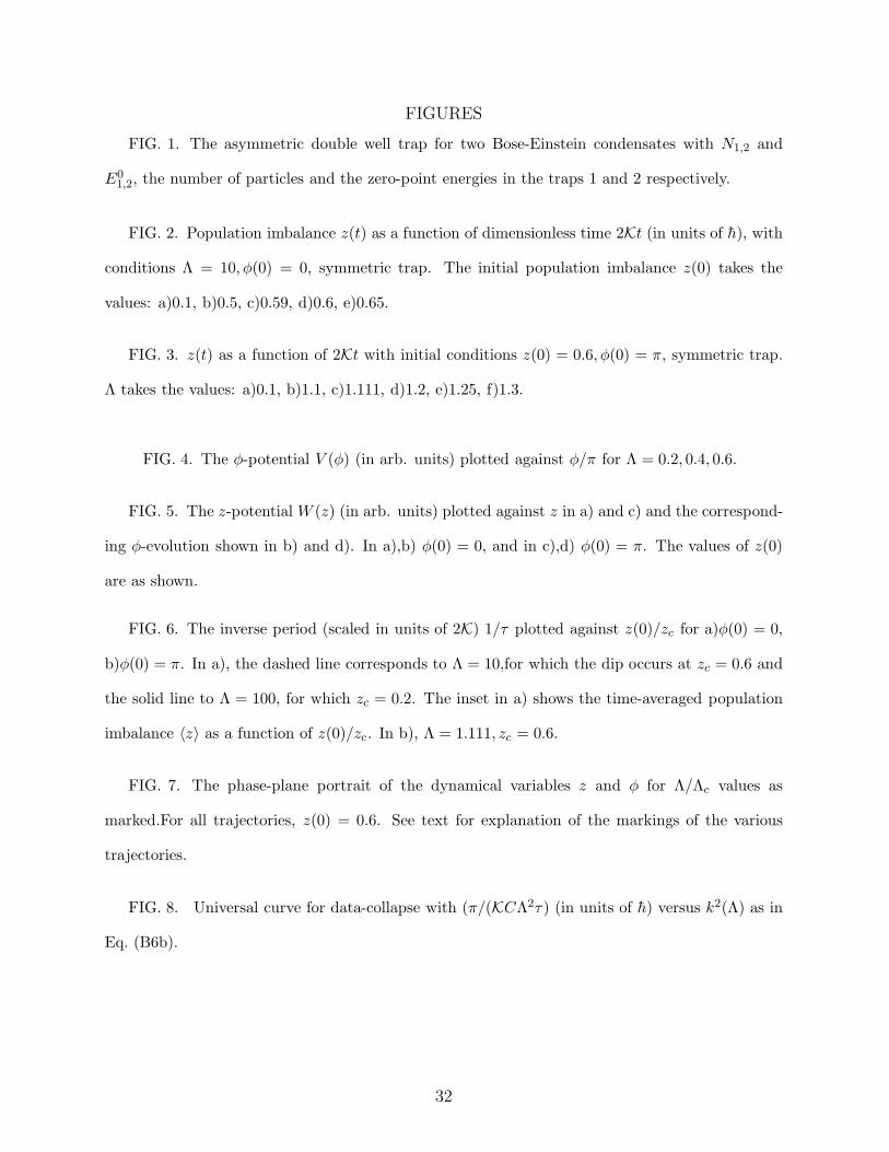
FIG. 1. The asymmetric double well trap for two Bose-Einstein condensates with N1,2 and

E01,2, the number of particles and the zero-point energies in the traps 1 and 2 respectively.

FIG. 2. Population imbalance z(t) as a function of dimensionless time 2Kt (in units of h), with

conditions Λ = 10, φ(0) = 0, symmetric trap. The initial population imbalance z(0) takes the

values: a)0.1, b)0.5, c)0.59, d)0.6, e)0.65.

FIG. 3. z(t) as a function of 2Kt with initial conditions z(0) = 0.6, φ(0) = π, symmetric trap.

Λ takes the values: a)0.1, b)1.1, c)1.111, d)1.2, e)1.25, f)1.3.

FIG. 4. The φ-potential V (φ) (in arb. units) plotted against φ/π for Λ = 0.2, 0.4, 0.6.

FIG. 5. The z-potential W (z) (in arb. units) plotted against z in a) and c) and the correspond-

ing φ-evolution shown in b) and d). In a),b) φ(0) = 0, and in c),d) φ(0) = π. The values of z(0)

are as shown.

FIG. 6. The inverse period (scaled in units of 2K) 1/τ plotted against z(0)/zc for a)φ(0) = 0,

b)φ(0) = π. In a), the dashed line corresponds to Λ = 10,for which the dip occurs at zc = 0.6 and

the solid line to Λ = 100, for which zc = 0.2. The inset in a) shows the time-averaged population

imbalance 〈z〉 as a function of z(0)/zc. In b), Λ = 1.111, zc = 0.6.

FIG. 7. The phase-plane portrait of the dynamical variables z and φ for Λ/Λc values as

marked.For all trajectories, z(0) = 0.6. See text for explanation of the markings of the various

trajectories.

FIG. 8. Universal curve for data-collapse with (π/(KCΛ2τ) (in units of h) versus k2(Λ) as in

Eq. (B6b).

32

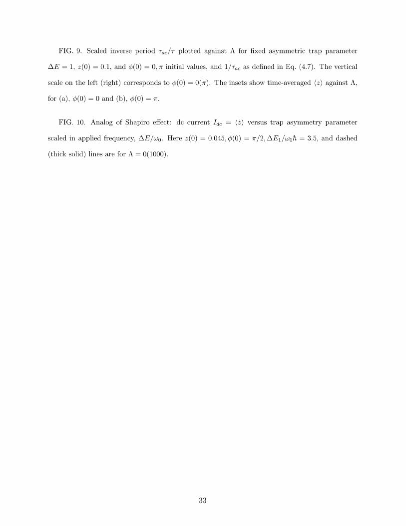
FIG. 9. Scaled inverse period τac/τ plotted against Λ for fixed asymmetric trap parameter

∆E = 1, z(0) = 0.1, and φ(0) = 0, π initial values, and 1/τac as defined in Eq. (4.7). The vertical

scale on the left (right) corresponds to φ(0) = 0(π). The insets show time-averaged 〈z〉 against Λ,

for (a), φ(0) = 0 and (b), φ(0) = π.

FIG. 10. Analog of Shapiro effect: dc current Idc = 〈z〉 versus trap asymmetry parameter

scaled in applied frequency, ∆E/ω0. Here z(0) = 0.045, φ(0) = π/2,∆E1/ω0h = 3.5, and dashed

(thick solid) lines are for Λ = 0(1000).

33

1 2

E1

E2

Pot

entia

l Ene

rgy

Distance

0

0

Fig.1

0 5 10−0.6

−0.3

0.0

0.3

0.6

z(t)

−0.10

−0.05

0.00

0.05

0.10

z(t)

0 5 10−0.4

0.0

0.4

0.8−0.6

−0.4

−0.2

0.0

0.2

0.4

0.6

time

e)

a) b)

c)

d)

0 10 20 30 40−0.6

−0.4

−0.2

0.0

0.2

0.4

0.6

z(t)

0 10 20 30 40−0.6

−0.4

−0.2

0.0

0.2

0.4

0.6z(

t)

0 10 20 30 400.0

0.2

0.4

0.6

0.8

1.0

0 10 20 30 40−0.6

−0.4

−0.2

0.0

0.2

0.4

0.6a) b)

c)

d)

e)

f)

time

−2 −1 0 1 2φ/π

V(φ

)

Λ=0.2

Λ=0.4

Λ=0.6

−1.0 −0.5 0.0 0.5 1.0−2.0

−1.0

0.0

1.0

2.0

−1.0 −0.5 0.0 0.5 1.0

a)

b)

c)

d)

z(0)=0.1

z(0)=0.7

z(0)=0.6

z(0)=0.5

z(0)=0.1

z(0)=0.5

z(0)=0.6

z(0)=0.7

z(0)=0.1

z(0)=0.1

z(0)=0.5

z(0)=0.7

z(0)=0.98

z(0)=0.5

z(0)=0.7

z(0)=0.98

φ(0)=π,Λ=2.5φ(0)=0,Λ=10

z z

φ/π

W(z

)

0.0 0.5 1.0 1.5z(0)/ zc

0.00

0.05

0.10

1/τ

0.0

1.0

2.0

3.0

4.0

5.0

1/τ

0.0 0.5 1.0 1.50.0

0.5

1.0φ(0)=0

φ(0)=π

Λ=100

zc=0.2

Λ=10

zc=0.6

Λ=1.1

zc=0.6

MQST

MQST

a)

b)

z(0)/zc

<z>

−2 −1 0 1 2φ/π

−1.0

−0.5

0.0

0.5

1.0

z 00.8

1

1.5

0

0.99

1.04

2

2.7

0.0 0.5 1.0 1.5 2.0k

2(Λ)

0

2

4

π/(K

CΛ

τ)

0.0 0.2 0.4 0.6 0.8 1.00

10

20

30

40

50

0.0 0.5 1.0−0.4

−0.2

0.0

0.2

0.4

0.0 0.5 1.0−0.4

−0.2

0.0

0.2

0.4

0

1

2

3

Λ/Λc(∆E) Λ/Λc(∆E)

∆E=1.0

<z(

t)>

Λ/Λc(∆E)

φ(0)=π

z(0)=0.1

τ ac/τ τ ac

/τ

<z(

t)>

(a) (b)

φ(0)=0

φ(0)=0 φ(0)=π

(Left scale)

(Right scale)

0 1 2 3 4 5 60.0

0.1

0.2

0.3

0.4

0.5

∆E/ω0

Idc

Λ=0

Λ=1000