9–1

9 Coherence Selection:Phase Cycling and Gradient Pulses†

9.1 Introduction

The pulse sequence used in an NMR experiment is carefully designed toproduce a particular outcome. For example, we may wish to pass the spinsthrough a state of multiple quantum coherence at a particular point, or plan forthe magnetization to be aligned along the z-axis during a mixing period.However, it is usually the case that the particular series of events we designedthe pulse sequence to cause is only one out of many possibilities. For example,a pulse whose role is to generate double-quantum coherence from anti-phasemagnetization may also generate zero-quantum coherence or transfer themagnetization to another spin. Each time a radiofrequency pulse is appliedthere is this possibility of branching into many different pathways. If no stepsare taken to suppress these unwanted pathways the resulting spectrum will behopelessly confused and uninterpretable.

There are two general ways in which one pathway can be isolated from themany possible. The first is phase cycling. In this method the phases of thepulses and the receiver are varied in a systematic way so that the signal fromthe desired pathways adds and signal from all other pathways cancels. Phasecycling requires that the experiment is repeated several times, something whichis probably required in any case in order to achieve the required signal-to-noiseratio.

The second method of selection is to use field gradient pulses. These areshort periods during which the applied magnetic field is made inhomogeneous.As a result, any coherences present dephase and are apparently lost. However,this dephasing can be undone, and the coherence restored, by application of asubsequent gradient. We shall see that this dephasing and rephasing approachcan be used to select particular coherences. Unlike phase cycling, the use offield gradient pulses does not require repetition of the experiment.

Both of these selection methods can be described in a unified frameworkwhich classifies the coherences present at any particular point according to acoherence order and then uses coherence transfer pathways to specify thedesired outcome of the experiment.

9.2 Phase in NMR

In NMR we have control over both the phase of the pulses and the receiverphase. The effect of changing the phase of a pulse is easy to visualise in theusual rotating frame. So, for example, a 90° pulse about the x-axis rotates

† Chapter 9 "Coherence Selection: Phase Cycling and Gradient Pulses" © James Keeler 2001

and 2003.

9–2

magnetization from z onto –y, whereas the same pulse applied about the y-axisrotates the magnetization onto the x-axis. The idea of the receiver phase isslightly more complex and will be explored in this section.

The NMR signal – that is the free induction decay – which emerges from theprobe is a radiofrequency signal oscillating at close to the Larmor frequency(usually hundreds of MHz). Within the spectrometer this signal is shifted downto a much lower frequency in order that it can be digitized and then stored incomputer memory. The details of this down-shifting process can be quitecomplex, but the overall result is simply that a fixed frequency, called thereceiver reference or carrier, is subtracted from the frequency of the incomingNMR signal. Frequently, this receiver reference frequency is the same as thetransmitter frequency used to generate the pulses applied to the observednucleus. We shall assume that this is the case from now on.

The rotating frame which we use to visualise the effect of pulses is set at thetransmitter frequency, ωrf, so that the field due to the radiofrequency pulse isstatic. In this frame, a spin whose Larmor frequency is ω0 precesses at (ω0 –ωrf), called the offset Ω. In the spectrometer the incoming signal at ω0 is down-shifted by subtracting the receiver reference which, as we have already decided,will be equal to the frequency of the radiofrequency pulses. So, in effect, thefrequencies of the signals which are digitized in the spectrometer are the offsetfrequencies at which the spins evolve in the rotating frame. Often this wholeprocess is summarised by saying that the "signal is detected in the rotatingframe".

9.2.1 Detector phase

The quantity which is actually detected in an NMR experiment is the transversemagnetization. Ultimately, this appears at the probe as an oscillating voltage,which we will write as

S tFID = cosω0

where ω0 is the Larmor frequency. The down-shifting process in thespectrometer is achieved by an electronic device called a mixer; this effectivelymultiplies the incoming signal by a locally generated reference signal, Sref,which we will assume is oscillating at ωrf

S tref rf= cosωThe output of the mixer is the product SFIDSref

S S A t t

A t t

FID ref rf

rf rf

=

= +( ) + −( )[ ]cos cos

cos cos

ω ω

ω ω ω ω0

12 0 0

The first term is an oscillation at a high frequency (of the order of twice theLarmor frequency as ω0 ≈ ωrf) and is easily removed by a low-pass filter. Thesecond term is an oscillation at the offset frequency, Ω. This is in line with theprevious comment that this down-shifting process is equivalent to detecting theprecession in the rotating frame.

9–3

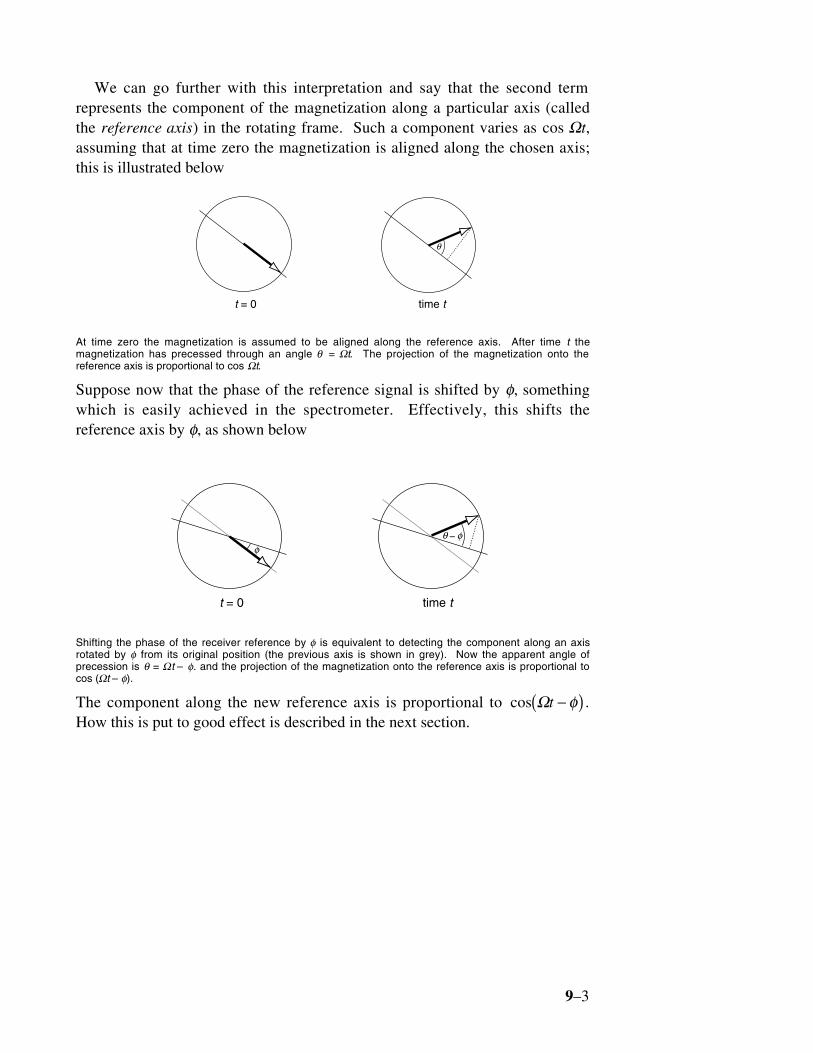
We can go further with this interpretation and say that the second termrepresents the component of the magnetization along a particular axis (calledthe reference axis) in the rotating frame. Such a component varies as cos Ωt,assuming that at time zero the magnetization is aligned along the chosen axis;this is illustrated below

θ

t = 0 time t

At time zero the magnetization is assumed to be aligned along the reference axis. After time t themagnetization has precessed through an angle θ = Ωt. The projection of the magnetization onto thereference axis is proportional to cos Ωt.

Suppose now that the phase of the reference signal is shifted by φ, somethingwhich is easily achieved in the spectrometer. Effectively, this shifts thereference axis by φ, as shown below

φ

t = 0 time t

θ φ–

Shifting the phase of the receiver reference by φ is equivalent to detecting the component along an axisrotated by φ from its original position (the previous axis is shown in grey). Now the apparent angle ofprecession is θ = Ωt – φ. and the projection of the magnetization onto the reference axis is proportional tocos (Ωt – φ).

The component along the new reference axis is proportional to cos Ωt −( )φ .How this is put to good effect is described in the next section.

9–4

9.2.2 Quadrature detection

We normally want to place the transmitter frequency in the centre of theresonances of interest so as to minimise off-resonance effects. If the receiverreference frequency is the same as the transmitter frequency, it immediatelyfollows that the offset frequencies, Ω , may be both positive and negative.However, as we have seen in the previous section the effect of the down-shifting scheme used is to generate a signal of the form cos Ωt. Since cos(θ) =cos(–θ) such a signal does not discriminate between positive and negativeoffset frequencies. The resulting spectrum, obtained by Fourier transformation,would be confusing as each peak would appear at both +Ω and –Ω.

The way out of this problem is to detect the signal along two perpendicularaxes. As is illustrated opposite, the projection along one axis is proportional tocos(Ωt) and to sin(Ωt) along the other. Knowledge of both of these projectionsenables us to work out the sense of rotation of the vector i.e. the sign of theoffset.

The sin modulated component is detected by having a second mixer fed witha reference whose phase is shifted by π/2. Following the above discussion theoutput of the mixer is

cos cos cos sin sin

sin

Ω Ω ΩΩ

t t t

t

−( ) = +=

π π π2 2 2

The output of these two mixers can be regarded as being the components of themagnetization along perpendicular axes in the rotating frame.

The final step in this whole process is regard the outputs of the two mixers asbeing the real and imaginary parts of a complex number:

cos sin expΩ Ω Ωt t t+ = ( )i i

The overall result is the generation of a complex signal whose phase variesaccording to the offset frequency Ω.

9.2.3 Control of phase

In the previous section we supposed that the signal coming from the probe wasof the form cosω 0t but it is more realistic to write the signal ascos(ω0t + φsig) in recognition of the fact that in addition to a frequency the signalhas a phase, φsig. This phase is a combination of factors that are not under ourcontrol (such as phase shifts produced in the amplifiers and filters throughwhich the signal passes) and a phase due to the pulse sequence, which certainlyis under our control.

The overall result of this phase is simply to multiply the final complex signalby a phase factor, exp(iφsig):

exp expi i sigΩt( ) ( )φ

As we saw in the previous section, we can also introduce another phase shift byaltering the phase of the reference signal fed to the mixer, and indeed we saw

θ x

y

The x and y projections of theblack vector are both positive.If the vector had precessed inthe opposite direction (shownshaded), and at the samefrequency, the projection alongx would be the same, but alongy it would be minus that of theblack vector.

9–5

that the cosine and sine modulated signals are generated by using two mixersfed with reference signals which differ in phase by π/2. If the phase of each ofthese reference signals is advanced by φrx, usually called the receiver phase, theoutput of the two mixers becomes cos Ωt −( )φrx and sin Ωt −( )φrx . In thecomplex notation, the overall signal thus acquires another phase factor

exp exp expi i isig rxΩt( ) ( ) −( )φ φ

Overall, then, the phase of the final signal depends on the difference betweenthe phase introduced by the pulse sequence and the phase introduced by thereceiver reference.

9.2.4 Lineshapes

Let us suppose that the signal can be written

S t B t t T( ) = ( ) ( ) −( )exp exp expi iΩ Φ 2

where Φ is the overall phase (= −φ φsig rx ) and B is the amplitude. The term,exp(-t/T2) has been added to impose a decay on the signal. Fouriertransformation of S(t) gives the spectrum S(ω):

S B A Dω ω ω( ) = ( ) + ( )[ ] ( )i iexp Φ [1]

where A(ω) is an absorption mode lorentzian lineshape centred at ω = Ω andD(ω) is the corresponding dispersion mode lorentzian:

AT

TD

T

Tω

ωω ω

ω( ) =

+ −( ) ( ) = −( )+ −( )

22

22

22

2221 1Ω

ΩΩ

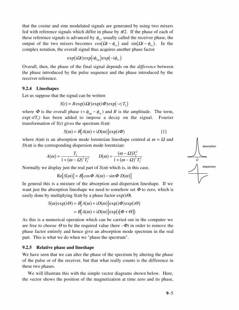
Normally we display just the real part of S(ω) which is, in this case,

Re cos sinS B A Dω ω ω( )[ ] = ( ) − ( )[ ]Φ ΦIn general this is a mixture of the absorption and dispersion lineshape. If wewant just the absorption lineshape we need to somehow set Φ to zero, which iseasily done by multiplying S(ω) by a phase factor exp(iΘ).

S B A D

B A D

ω ω ω

ω ω

( ) ( ) = ( ) + ( )[ ] ( ) ( )= ( ) + ( )[ ] +[ ]( )

exp exp exp

exp

i i i i

i i

Θ Φ Θ

Φ Θ

As this is a numerical operation which can be carried out in the computer weare free to choose Θ to be the required value (here –Φ) in order to remove thephase factor entirely and hence give an absorption mode spectrum in the realpart. This is what we do when we "phase the spectrum".

9.2.5 Relative phase and lineshape

We have seen that we can alter the phase of the spectrum by altering the phaseof the pulse or of the receiver, but that what really counts is the difference inthese two phases.

We will illustrate this with the simple vector diagrams shown below. Here,the vector shows the position of the magnetization at time zero and its phase,

absorption

dispersion

Ω

9–6

φsig, is measured anti-clockwise from the x-axis. The dot shows the axis alongwhich the receiver is aligned; this phase, φrx, is also measured anti-clockwisefrom the x-axis.

If the vector and receiver are aligned along the same axis, Φ = 0, and the realpart of the spectrum shows the absorption mode lineshape. If the receiverphase is advanced by π/2, Φ = 0 – π/2 and, from Eq. [1]

S B A D

B A D

ω ω ω π

ω ω

( ) = ( ) + ( )[ ] −( )= − ( ) + ( )[ ]

i i

i

exp 2

This means that the real part of the spectrum shows a dispersion lineshape. Onthe other hand, if the magnetization is advanced by π/2, Φ = φ sig – φ r x

= π/2 – 0 = π/2 and it can be shown from Eq. [1] that the real part of thespectrum shows a negative dispersion lineshape. Finally, if either phase isadvanced by π, the result is a negative absorption lineshape.

x

y

φrx φ

9.2.6 CYCLOPS

The CYCLOPS phase cycling scheme is commonly used in even the simplestpulse-acquire experiments. The sequence is designed to cancel someimperfections associated with errors in the two phase detectors mentionedabove; a description of how this is achieved is beyond the scope of thisdiscussion. However, the cycle itself illustrates very well the points made inthe previous section.

There are four steps in the cycle, the pulse phase goes x, y, –x, –y i.e. itadvances by 90° on each step; likewise the receiver advances by 90° on eachstep. The figure below shows how the magnetization and receiver phases arerelated for the four steps of this cycle

9–7

x–x

y

–y

pulse x y –x –y

receiver x y –x –y

Although both the receiver and the magnetization shift phase on each step, thephase difference between them remains constant. Each step in the cycle thusgives the same lineshape and so the signal adds on all four steps, which is justwhat is required.

Suppose that we forget to advance the pulse phase; the outcome is quitedifferent

x–x

y

–y

pulse x x x x

receiver x y –x –y

Now the phase difference between the receiver and the magnetization is nolonger constant. A different lineshape thus results from each step and it is clearthat adding all four together will lead to complete cancellation (steps 2 and 4cancel, as do steps 1 and 3). For the signal to add up it is clearly essential forthe receiver to follow the magnetization.

9.2.7 EXORCYLE

EXORCYLE is perhaps the original phase cycle. It is a cycle used for 180°pulses when they form part of a spin echo sequence. The 180° pulse cyclesthrough the phases x, y, –x, –y and the receiver phase goes x, –x, x, –x. Thediagram below illustrates the outcome of this sequence

9–8

x–x

y

y

–y

–y

90°(x) –

180°(±x)

180°(±y)

τ

τ

τ

If the phase of the 180° pulse is +x or –x the echo forms along the y-axis,whereas if the phase is ±y the echo forms on the –y axis. Therefore, as the 180°pulse is advanced by 90° (e.g. from x to y) the receiver must be advanced by180° (e.g. from x to –x). Of course, we could just as well cycle the receiverphases y, –y, y, –y; all that matters is that they advance in steps of 180°. Wewill see later on how it is that this phase cycle cancels out the results ofimperfections in the 180° pulse.

9.2.8 Difference spectroscopy

Often a simple two step sequence suffices to cancel unwanted magnetization;essentially this is a form of difference spectroscopy. The idea is well illustratedby the INEPT sequence, shown opposite. The aim of the sequence is to transfermagnetization from spin I to a coupled spin S.

With the phases and delays shown equilibrium magnetization of spin I, Iz, istransferred to spin S, appearing as the operator Sx. Equilibrium magnetizationof S, Sz, appears as Sy. We wish to preserve only the signal that has beentransferred from I.

The procedure to achieve this is very simple. If we change the phase of thesecond I spin 90° pulse from y to –y the magnetization arising from transfer ofthe I spin magnetization to S becomes –Sx i.e. it changes sign. In contrast, thesignal arising from equilibrium S spin magnetization is unaffected simplybecause the Sz operator is unaffected by the I spin pulses. By repeating theexperiment twice, once with the phase of the second I spin 90° pulse set to yand once with it set to –y, and then subtracting the two resulting signals, theundesired signal is cancelled and the desired signal adds. It is easily confirmedthat shifting the phase of the S spin 90° pulse does not achieve the desiredseparation of the two signals as both are affected in the same way.

In practice the subtraction would be carried out by shifting the receiver by180°, so the I spin pulse would go y, –y and the receiver phase go x, –x. This isa two step phase cycle which is probably best viewed as differencespectroscopy.

This simple two step cycle is the basic element used in constructing the

I

S

y

2J1

2J1

Pulse sequence for INEPT.Filled rectangles represent 90°pulses and open rectanglesrepresent 180° pulses. Unlessotherwise indicated, all pulsesare of phase x.

9–9

phase cycling of many two- and three-dimensional heteronuclear experiments.

9.3 Coherence transfer pathways

Although we can make some progress in writing simple phase cycles byconsidering the vector picture, a more general framework is needed in order tocope with experiments which involve multiple-quantum coherence and relatedphenomena. We also need a theory which enables us to predict the degree towhich a phase cycle can discriminate against different classes of unwantedsignals. A convenient and powerful way of doing both these things is to use thecoherence transfer pathway approach.

9.3.1 Coherence order

Coherences, of which transverse magnetization is one example, can beclassified according to a coherence order, p, which is an integer taking values 0,± 1, ± 2 ... Single quantum coherence has p = ± 1, double hasp = ± 2 and so on; z-magnetization, "zz" terms and zero-quantum coherencehave p = 0. This classification comes about by considering the phase whichdifferent coherences acquire is response to a rotation about the z-axis.

A coherence of order p, represented by the density operator σ p( ) , evolvesunder a z-rotation of angle φ according to

exp exp exp−( ) ( ) = −( )( ) ( )i i iφ σ φ φ σF F pzp

zp [2]

where Fz is the operator for the total z-component of the spin angularmomentum. In words, a coherence of order p experiences a phase shift of –pφ.Equation [2] is the definition of coherence order.

To see how this definition can be applied, consider the effect of a z-rotationon transverse magnetization aligned along the x-axis. Such a rotation isidentical in nature to that due to evolution under an offset, and using productoperators it can be written

exp exp cos sin−( ) ( ) = +i iφ φ φ φI I I I Iz x z x y [3]

The right hand sides of Eqs. [2] and [3] are not immediately comparable, but bywriting the sine and cosine terms as complex exponentials the comparisonbecomes clearer. Using

cos exp exp exp expφ φ φ φ φ φ= ( ) + −( )[ ] = ( ) − −( )[ ]12

12i i in i iis

Eq. [3] becomes

exp exp

exp exp exp exp

exp exp

−( ) ( )= ( ) + −( )[ ] + ( ) − −( )[ ]= +[ ] ( ) + −[ ] −( )

i i

i i i i

i i

i

i i

φ φ

φ φ φ φ

φ φ

I I I

I I

I I I I

z x z

x y

x y x y

12

12

12

1 12

1

It is now clear that the first term corresponds to coherence order –1 and thesecond to +1; in other words, Ix is an equal mixture of coherence orders ±1.

The cartesian product operators do not correspond to a single coherence

9–10

order so it is more convenient to rewrite them in terms of the raising andlowering operators, I+ and I–, defined as

I I I I I Ix y x y+ = + =i i– –

from which it follows thatI I I I I Ix = +[ ] = −[ ]+ +

12

12– – y i [4]

Under z-rotations the raising and lowering operators transform simply

exp exp exp−( ) ( ) = ( )± ±i i iφ φ φI I I Iz z m

which, by comparison with Eq. [2] shows that I+ corresponds to coherenceorder +1 and I– to –1. So, from Eq. [4] we can see that Ix and Iy correspond tomixtures of coherence orders +1 and –1.

As a second example consider the pure double quantum operator for twocoupled spins,

2 21 2 1 2I I I Ix y y x+

Rewriting this in terms of the raising and lowering operators gives

11 2 1 2i I I I I+ + − −−( )

The effect of a z-rotation on the term I I1 2+ + is found as follows:

exp exp exp exp

exp exp exp

exp exp exp

−( ) −( ) ( ) ( )= −( ) −( ) ( )= −( ) −( ) = −( )

+ +

+ +

+ + + +

i i i i

i i i

i i i

φ φ φ φ

φ φ φ

φ φ φ

I I I I I I

I I I I

I I I I

z z z z

z z

1 2 1 2 2 1

1 1 2 1

1 2 1 22

Thus, as the coherence experiences a phase shift of –2φ the coherence isclassified according to Eq. [2] as having p = 2. It is easy to confirm that theterm I I1 2− − has p = –2. Thus the pure double quantum term, 2 21 2 1 2I I I Ix y y x+ , isan equal mixture of coherence orders +2 and –2.

As this example indicates, it is possible to determine the order or orders ofany state by writing it in terms of raising and lowering operators and thensimply inspecting the number of such operators in each term. A raisingoperator contributes +1 to the coherence order whereas a lowering operatorcontributes –1. A z-operator, Iiz, has coherence order 0 as it is invariant to z-rotations.

Coherences involving heteronuclei can be assigned both an overall order andan order with respect to each nuclear species. For example the term I S1 1+ –

hasan overall order of 0, is order +1 for the I spins and –1 for the S spins. The termI I S z1 2 1+ + is overall of order 2, is order 2 for the I spins and is order 0 for the Sspins.

9.3.2 Evolution under offsets

The evolution under an offset, Ω , is simply a z-rotation, so the raising andlowering operators simply acquire a phase Ωt

9–11

exp exp exp−( ) ( ) = ( )± ±i i iΩ Ω ΩtI I tI t Iz z m

For products of these operators, the overall phase is the sum of the phasesacquired by each term

exp exp exp exp

exp

−( ) −( ) ( ) ( )= −( )( )

− +

− +

i i i i

i

Ω Ω Ω Ω

Ω Ω

j jz i iz i j i iz j jz

i j i j

tI tI I I tI tI

t I I

It also follows that coherences of opposite sign acquire phases of opposite signsunder free evolution. So the operator I1+I2+ (with p = 2) acquires a phase –(Ω1 +Ω2)t i.e. it evolves at a frequency –(Ω1 + Ω2) whereas the operator I1–I2– (with p= –2) acquires a phase (Ω1 + Ω2)t i.e. it evolves at a frequency (Ω1 + Ω2). Wewill see later on that this observation has important consequences for thelineshapes in two-dimensional NMR.

The observation that coherences of different orders respond differently toevolution under a z-rotation (e.g. an offset) lies at the heart of the way in whichgradient pulses can be used to separate different coherence orders.

9.3.3 Phase shifted pulses

In general, a radiofrequency pulse causes coherences to be transferred from oneorder to one or more different orders; it is this spreading out of the coherencewhich makes it necessary to select one transfer among many possibilities. Anexample of this spreading between coherence orders is the effect of a non-selective pulse on antiphase magnetization, such as 2I1xI2z, which corresponds tocoherence orders ±1. Some of the coherence may be transferred into double-and zero-quantum coherence, some may be transferred into two-spin order andsome will remain unaffected. The precise outcome depends on the phase andflip angle of the pulse, but in general we can see that there are manypossibilities.

If we consider just one coherence, of order p , being transferred to acoherence of order p' by a radiofrequency pulse we can derive a very generalresult for the way in which the phase of the pulse affects the phase of thecoherence. It is on this relationship that the phase cycling method is based.

We will write the initial state of order p as σ p( ) , and the final state of order p'as σ p'( ) . The effect of the radiofrequency pulse causing the transfer isrepresented by the (unitary) transformation Uφ where φ is the phase of thepulse. The initial and final states are related by the usual transformation

U Up p0 0

1σ σ( ) ( )= +– ' terms of other orders [5]

which has been written for phase 0; the other terms will be dropped as we areonly interested in the transfer from p to p'. The transformation brought aboutby a radiofrequency pulse phase shifted by φ, Uφ, is related to that with thephase set to zero, U0, in the following way

U F U Fz zφ φ φ= −( ) ( )exp expi i0 [6]

9–12

Using this, the effect of the phase shifted pulse on the initial state σ p( ) can bewritten

U U

F U F F U F

p

z zp

z z

φ φσ

φ φ σ φ φ

( )

( )= −( ) ( ) −( ) ( )

–

–exp exp exp exp

1

0 01i i i i

[7]

The central three terms can be simplified by application of Eq. [2]

exp exp exp–i i iφ σ φ φ σF F U pzp

zp( ) −( ) = ( )( ) ( )

01

giving

U U p F U U Fpz

pzφ φσ φ φ σ φ( ) ( )= ( ) −( ) ( )– –exp exp exp1

0 01i i i

The central three terms can, from Eq. [5], be replaced by σ p'( ) to give

U U p F Fpz

pzφ φσ φ φ σ φ( ) ( )= ( ) −( ) ( )– 'exp exp exp1 i i i

Finally, Eq. [5] is applied again to give

U U p pp pφ φσ φ φ σ( ) ( )= ( ) ( )– 'exp exp '1 i –i

Defining ∆p = (p' – p) as the change is coherence order, this simplifies to

U U pp pφ φσ φ σ( ) ( )= ( )– 'exp –1 i∆ [8]

Equation [8] says that if the phase of a pulse which is causing a change incoherence order of ∆p is shifted by φ the coherence will acquire a phase label(–∆p φ). It is this property which enables us to separate different changes incoherence order from one another by altering the phase of the pulse.

In the discussion so far it has been assumed that Uφ represents a single pulse.However, any sequence of pulses and delays can be represented by a singleunitary transformation, so Eq. [8] applies equally well to the effect of phaseshifting all of the pulses in such a sequence. We will see that this property isoften of use in writing phase cycles.

If a series of phase shifted pulses (or pulse sandwiches) are applied a phase(–∆p φ) is acquired from each. The total phase is found by adding up theseindividual contributions. In an NMR experiment this total phase affects thesignal which is recorded at the end of the sequence, even though the phase shiftmay have been acquired earlier in the pulse sequence. These phase shifts are,so to speak, carried forward.

9.3.4 Coherence transfer pathways diagrams

In designing a multiple-pulse NMR experiment the intention is to have specificorders of coherence present at various points in the sequence. One way ofindicating this is to use a coherence transfer pathway (CTP) diagram alongwith the timing diagram for the pulse sequence. An example of shown below,which gives the pulse sequence and CTP for the DQF COSY experiment.

9–13

t1 t2

210

–1–2

p

∆p=±1 ±1,±3+1,–3

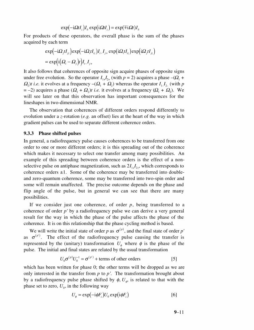
The solid lines under the sequence represent the coherence orders requiredduring each part of the sequence; note that it is only the pulses which cause achange in the coherence order. In addition, the values of ∆p are shown for eachpulse. In this example, as is commonly the case, more than one order ofcoherence is present at a particular time. Each pulse is required to causedifferent changes to the coherence order – for example the second pulse isrequired to bring about no less than four values of ∆p. Again, this is a commonfeature of pulse sequences.

It is important to realise that the CTP specified with the pulse sequence isjust the desired pathway. We would need to establish separately (for exampleusing a product operator calculation) that the pulse sequence is indeed capableof generating the coherences specified in the CTP. Also, the spin system whichwe apply the sequence to has to be capable of supporting the coherences. Forexample, if there are no couplings, then no double quantum will be generatedand thus selection of the above pathway will result in a null spectrum.

The coherence transfer pathway must start with p = 0 as this is the order towhich equilibrium magnetization (z-magnetization) belongs. In addition, thepathway has to end with |p| = 1 as it is only single quantum coherence that isobservable. If we use quadrature detection (section 9.2.2) it turns out that onlyone of p = ±1 is observable; we will follow the usual convention of assumingthat p = –1 is the detectable signal.

9.4 Lineshapes and frequency discrimination

9.4.1 Phase and amplitude modulation

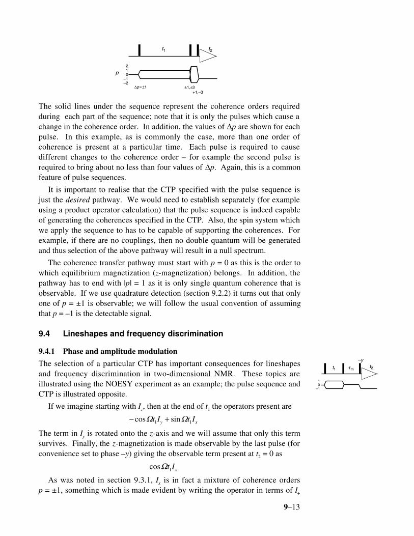
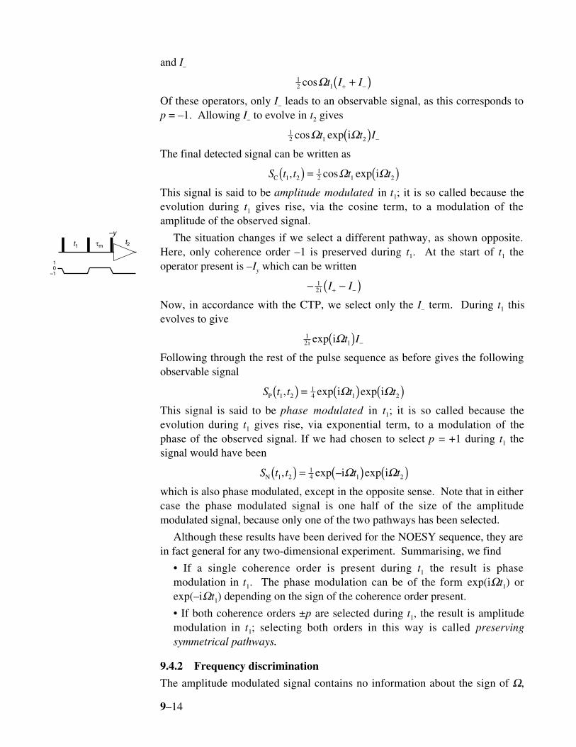
The selection of a particular CTP has important consequences for lineshapesand frequency discrimination in two-dimensional NMR. These topics areillustrated using the NOESY experiment as an example; the pulse sequence andCTP is illustrated opposite.

If we imagine starting with Iz, then at the end of t1 the operators present are

− +cos sinΩ Ωt I t Iy x1 1

The term in Iy is rotated onto the z-axis and we will assume that only this termsurvives. Finally, the z-magnetization is made observable by the last pulse (forconvenience set to phase –y) giving the observable term present at t2 = 0 as

cosΩt Ix1

As was noted in section 9.3.1, Ix is in fact a mixture of coherence ordersp = ±1, something which is made evident by writing the operator in terms of I+

t1 t2

10

–1

τm

–y

9–14

and I–

12 1cosΩt I I+ −+( )

Of these operators, only I– leads to an observable signal, as this corresponds top = –1. Allowing I– to evolve in t2 gives

12 1 2cos expΩ Ωt t Ii( ) −

The final detected signal can be written as

S t t t tC i1 212 1 2, cos exp( ) = ( )Ω Ω

This signal is said to be amplitude modulated in t1; it is so called because theevolution during t1 gives rise, via the cosine term, to a modulation of theamplitude of the observed signal.

The situation changes if we select a different pathway, as shown opposite.Here, only coherence order –1 is preserved during t1. At the start of t1 theoperator present is –Iy which can be written

− −( )+ −12i I I

Now, in accordance with the CTP, we select only the I– term. During t1 thisevolves to give

12 1i iexp Ωt I( ) −

Following through the rest of the pulse sequence as before gives the followingobservable signal

S t t t tP i i1 214 1 2, exp exp( ) = ( ) ( )Ω Ω

This signal is said to be phase modulated in t1; it is so called because theevolution during t1 gives rise, via exponential term, to a modulation of thephase of the observed signal. If we had chosen to select p = +1 during t1 thesignal would have been

S t t t tN –i i1 214 1 2, exp exp( ) = ( ) ( )Ω Ω

which is also phase modulated, except in the opposite sense. Note that in eithercase the phase modulated signal is one half of the size of the amplitudemodulated signal, because only one of the two pathways has been selected.

Although these results have been derived for the NOESY sequence, they arein fact general for any two-dimensional experiment. Summarising, we find

• If a single coherence order is present during t1 the result is phasemodulation in t1. The phase modulation can be of the form exp(iΩt1) orexp(–iΩt1) depending on the sign of the coherence order present.

• If both coherence orders ±p are selected during t1, the result is amplitudemodulation in t1; selecting both orders in this way is called preservingsymmetrical pathways.

9.4.2 Frequency discrimination

The amplitude modulated signal contains no information about the sign of Ω,

t1 t2

10

–1

τm

–y

9–15

simply because cos(Ωt1) = cos(–Ωt1). As a consequence, Fouriertransformation of the time domain signal will result in each peak appearingtwice in the two-dimensional spectrum, once at F1 = +Ω and once at F1 = –Ω.As was commented on above, we usually place the transmitter in the middle ofthe spectrum so that there are peaks with both positive and negative offsets. If,as a result of recording an amplitude modulated signal, all of these appeartwice, the spectrum will hopelessly confused. A spectrum arising from anamplitude modulated signal is said to lack frequency discrimination in F1.

On the other hand, the phase modulated signal is sensitive to the sign of theoffset and so information about the sign of Ω in the F1 dimension is containedin the signal. Fourier transformation of the signal SP(t1,t2) gives a peak at F1 =+Ω, F2 = Ω, whereas Fourier transformation of the signal SN(t1,t2) gives a peakat F1 = –Ω, F2 = Ω. Both spectra are said to be frequency discriminated as thesign of the modulation frequency in t1 is determined; in contrast to amplitudemodulated spectra, each peak will only appear once.

The spectrum from SP(t1,t2) is called the P-type (P for positive) or echospectrum; a diagonal peak appears with the same sign of offset in eachdimension. The spectrum from SN(t1,t2) is called the N-type (N for negative) oranti-echo spectrum; a diagonal peak appears with opposite signs in the twodimensions.

It might appear that in order to achieve frequency discrimination we shoulddeliberately select a CTP which leads to a P– or an N-type spectrum. However,such spectra show a very unfavourable lineshape, as discussed in the nextsection.

9.4.3 Lineshapes

In section 9.2.4 we saw that Fourier transformation of the signal

S t t t T( ) = ( ) −( )exp expiΩ 2

gave a spectrum whose real part is an absorption lorentzian and whoseimaginary part is a dispersion lorentzian:

S A Dω ω ω( ) = ( ) + ( )i

We will use the shorthand that A2 represents an absorption mode lineshape at F2

= Ω and D2 represents a dispersion mode lineshape at the same frequency.Likewise, A1+ represents an absorption mode lineshape at F1 = +Ω and D1+

represents the corresponding dispersion lineshape. A1– and D1– represent thecorresponding lines at F1 = –Ω.

The time domain signal for the P-type spectrum can be written as

S t t t t t T t TP i i1 214 1 2 1 2 2 2, exp exp exp exp( ) = ( ) ( ) −( ) −( )Ω Ω

where the damping factors have been included as before. Fouriertransformation with respect to t2 gives

S t F t t T A DP i i1 214 1 1 2 2 2, exp exp( ) = ( ) −( ) +[ ]Ω

9–16

and then further transformation with respect to t1 gives

S F F A D A DP i i1 214 1 1 2 2,( ) = +[ ] +[ ]+ +

The real part of this spectrum is

Re ,S F F A A D DP 1 214 1 2 1 2( ) = −[ ]+ +

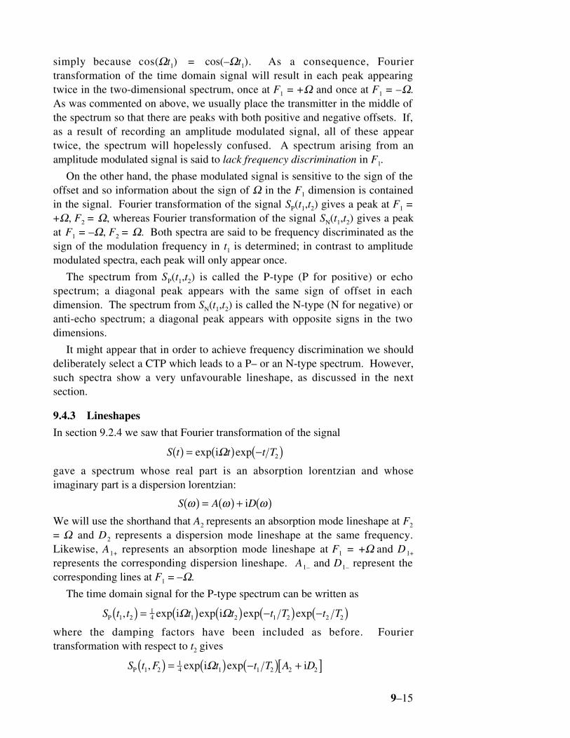
The quantity in the square brackets on the right represents a phase-twistlineshape at F1 = +Ω, F2 = Ω

Perspective view and contour plot of the phase-twist lineshape. Negative contours are shown dashed.

This lineshape is an inextricable mixture of absorption and dispersion, and it isvery undesirable for high-resolution NMR. So, although a phase modulatedsignal gives us frequency discrimination, which is desirable, it also results in aphase-twist lineshape, which is not.

The time domain signal for the amplitude modulated data set can be writtenas

S t t t t t T t TC i1 212 1 2 1 2 2 2, cos exp exp exp( ) = ( ) ( ) −( ) −( )Ω Ω

Fourier transformation with respect to t2 gives

S t F t t T A DC i1 212 1 1 2 2 2, cos exp( ) = ( ) −( ) +[ ]Ω

which can be rewritten as

S t F t t t T A DC i i i1 214 1 1 1 2 2 2, exp exp exp( ) = ( ) + −( )[ ] −( ) +[ ]Ω Ω

Fourier transformation with respect to t1 gives, in the real part of the spectrum

Re , – – –S F F A A D D A A D DC +1 214 1 2 1 2

14 1 2 1 2( ) = [ ] + [ ]+ −

This corresponds to two phase-twist lineshapes, one at F1 = +Ω, F2 = Ω and theother at F1 = –Ω, F2 = Ω; the lack of frequency discrimination is evident.Further, the undesirable phase-twist lineshape is again present.

The lineshape can be restored to the absorption mode by discarding theimaginary part of the time domain signal after the transformation with respectto t2, i.e. by taking the real part

Re , cos expS t F t t T AC 1 212 1 1 2 2( ) = ( ) −( )Ω

Subsequent transformation with respect to t1 gives, in the real part

9–17

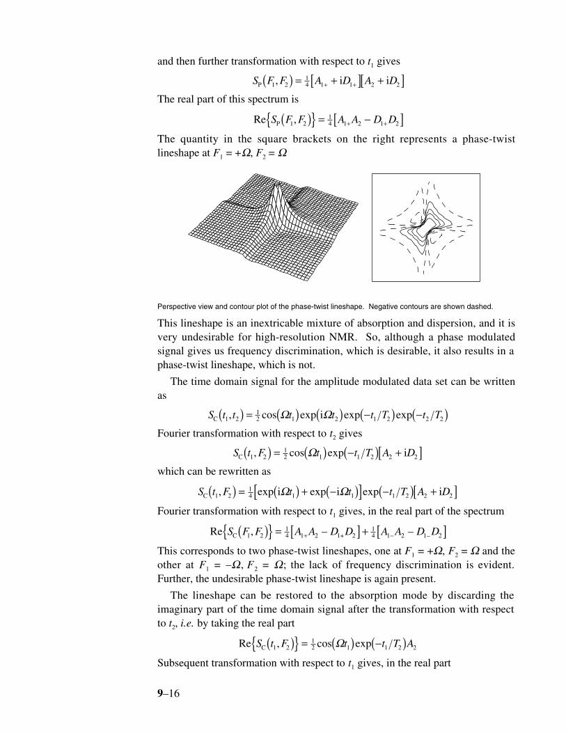
14 1 2

14 1 2A A A A+ −+

which is two double absorption mode lineshapes. Frequency discrimination islacking, but the lineshape is now much more desirable. The spectra with thetwo phase-twist and two absorption mode lines are shown below on the left andright, respectively.

0

F1

F2

0

F1

F2

9.4.4 Frequency discrimination with retention of absorption modelineshapes

For practical purposes it is essential to be able to achieve frequencydiscrimination and at the same time retain the absorption mode lineshape.There are a number of ways of doing this.

9.4.4.1 States-Haberkorn-Ruben (SHR) method

The key to this method is the ability to record a cosine modulated data set and asine modulated data set. The latter can be achieved simply by changing thephase of appropriate pulses. For example, in the case of the NOESYexperiment, all that is required to generate the sine data set is to shift the phaseof the first 90° pulse by 90° (in fact in the NOESY sequence the pulse needs toshift from x to –y). The two data sets have to kept separate.

The cosine data set is transformed with respect to t1 and the imaginary partdiscarded to give

Re , cos expS t F t t T AC 1 212 1 1 2 2( ) = ( ) −( )Ω [9]

The same operation is performed on the sine modulated data set

S t t t t t T t TS i1 212 1 2 1 2 2 2, sin exp exp exp( ) = ( ) ( ) −( ) −( )Ω Ω

Re , sin expS t F t t T AS 1 212 1 1 2 2( ) = ( ) −( )Ω [10]

A new complex data set is now formed by using the signal from Eq. [9] as thereal part and that from Eq. [10] as the imaginary part

S t F S t F S t F

t t T A

SHR C Si

i

1 2 1 2 1 2

12 1 1 2 2

, Re , Re ,

exp exp

( ) = ( ) + ( ) = ( ) −( )Ω

Fourier transformation with respect to t1 gives, in the real part of the spectrum

Re ,S F F A ASHR 1 212 1 2( ) = +

This is the desired frequency discriminated spectrum with a pure absorption

9–18

lineshape.

As commented on above, in NOESY all that is required to change fromcosine to sine modulation is to shift the phase of the first pulse by 90°. Thegeneral recipe is to shift the phase of all the pulses that precede t1 by 90°/|p1|,where p1 is the coherence order present during t1. So, for a double quantumspectrum, the phase shift needs to be 45°. The origin of this rule is that, takentogether, the pulses which precede t1 give rise to a pathway with ∆p = p1.

In heteronuclear experiments it is not usually necessary to shift the phase ofall the pulses which precede t1; an analysis of the sequence usually shows thatshifting the phase of the pulse which generates the transverse magnetizationwhich evolves during t1 is sufficient.

9.4.4.2 Echo anti-echo method

We will see in later sections that when we use gradient pulses for coherenceselection the natural outcome is P- or N-type data sets. Individually, each ofthese gives a frequency discriminated spectrum, but with the phase-twistlineshape. We will show in this section how an absorption mode lineshape canbe obtained provided both the P- and the N-type data sets are available.

As before, we write the two data sets as

S t t t t t T t T

S t t t t t T t T

P

N

i i

i i

1 214 1 2 1 2 2 2

1 214 1 2 1 2 2 2

, exp exp exp exp

, exp exp exp exp

( ) = ( ) ( ) −( ) −( )( ) = −( ) ( ) −( ) −( )

Ω Ω

Ω Ω

We then form the two combinations

S t t S t t S t t

t t t T t T

S t t S t t S t t

t t t T

C P N

S i P N

i

i

1 2 1 2 1 2

12 1 2 1 2 2 2

1 21

1 2 1 2

12 1 2 1 2

, , ,

cos exp exp exp

, , ,

sin exp exp

( ) = ( ) + ( )= ( ) ( ) −( ) −( )

( ) = ( ) + ( )[ ]= ( ) ( ) −

Ω Ω

Ω Ω (( ) −( )exp t T2 2

These cosine and sine modulated data sets can be used as inputs to the SHRmethod described in the previous section.

An alternative is to Fourier transform the two data sets with respect to t2 togive

S t F t t T A D

S t F t t T A D

P

N

i i

i i

1 214 1 1 2 2 2

1 214 1 1 2 2 2

, exp exp

, exp – exp

( ) = ( ) −( ) +[ ]( ) = ( ) −( ) +[ ]

Ω

Ω

We then take the complex conjugate of SN(t1,F2) and add it to SP(t1,F2)

S t F t t T A D

S t F S t F S t F

t t T A

N

N P

i i

i

1 214 1 1 2 2 2

1 2 1 2 1 2

12 1 1 2 2

, * exp exp

, , * ,

exp exp

( ) = ( ) −( ) −[ ]( ) = ( ) + ( )

= ( ) −( )+

Ω

Ω

Transformation of this signal gives

9–19

S F F A D A+ + +( ) = +[ ]1 212 1 1 2, i

which is frequency discriminated and has, in the real part, the required doubleabsorption lineshape.

9.4.4.3 Marion-Wüthrich or TPPI method

The idea behind the TPPI (time proportional phase incrementation) orMarion–Wüthrich (MW) method is to arrange things so that all of the peakshave positive offsets. Then, frequency discrimination is not required as there isno ambiguity.

One simple way to make all offsets positive is to set the receiver carrierfrequency deliberately at the edge of the spectrum. Simple though this is, it isnot really a very practical method as the resulting spectrum would be veryinefficient in its use of data space and in addition off-resonance effectsassociated with the pulses in the sequence will be accentuated.

In the TPPI method the carrier can still be set in the middle of the spectrum,but it is made to appear that all the frequencies are positive by phase shiftingsome of the pulses in the sequence in concert with the incrementation of t1.

It was noted above that shifting the phase of the first pulse in the NOESYsequence from x to –y caused the modulation to change from cos(Ωt1) tosin(Ωt1). One way of expressing this is to say that shifting the pulse causes aphase shift φ in the signal modulation, which can be written cos(Ωt1 + φ).Using the usual trigonometric expansions this can be written

cos cos cos sin sinΩ Ω Ωt t t1 1 1+( ) = −φ φ φIf the phase shift, φ, is –π/2 radians the result is

cos cos cos sin sin

sin

Ω Ω ΩΩ

t t t

t1 1 1

1

2 2 2+( ) = −( ) − −( )=

π π π

This is exactly the result we found before.

In the TPPI procedure, the phase φ is made proportional to t1 i.e. each time t1

is incremented, so is the phase. We will suppose that

φ ωt t1 1( ) = add

The constant of proportion between the time dependent phase, φ(t1), and t1 hasbeen written ω add; ω add has the dimensions of rad s– 1 i.e. it is a frequency.Following the same approach as before, the time-domain function with theinclusion of this incrementing phase is thus

cos cos

cos

Ω Ω

Ω

t t t t

t

1 1 1 1

1

+ ( )( ) = +( )= +( )

φ ω

ωadd

add

In words, the effect of incrementing the phase in concert with t1 is to add afrequency ωadd to all of the offsets in the spectrum. The TPPI method utilizesthis in the following way.

In one-dimensional pulse-Fourier transform NMR the free induction signal is

9–20

sampled at regular intervals ∆. After transformation the resulting spectrumdisplays correctly peaks with offsets in the range –(SW/2) to +(SW/2) where SWis the spectral width which is given by 1/∆ (this comes about from the Nyquisttheorem of data sampling). Frequencies outside this range are not representedcorrectly.

Suppose that the required frequency range in the F1 dimension is from–(SW1/2) to +(SW1/2). To make it appear that all the peaks have a positiveoffset, it will be necessary to add (SW1/2) to all the frequencies. Then the peakswill be in the range 0 to (SW1).

As the maximum frequency is now (SW1) rather than (SW1/2) the samplinginterval, ∆1, will have to be halved i.e. ∆1 = 1/(2SW1) in order that the range offrequencies present are represented properly.

The phase increment is ωaddt1 , but t1 can be written as n∆ 1 for the nthincrement of t1. The required value for ωadd is 2π(SW1/2) , where the 2π is toconvert from frequency (the units of SW1) to rad s–1, the units of ωadd . Puttingall of this together ωaddt1 can be expressed, for the nth increment as

ω π

π

π

additionaltSW

n

SWn

SW

n

11

1

1

1

22

22

1

2

2

=

( )

=

=

∆

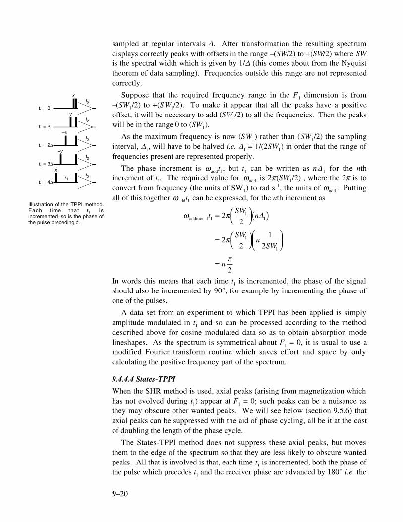
In words this means that each time t1 is incremented, the phase of the signalshould also be incremented by 90°, for example by incrementing the phase ofone of the pulses.

A data set from an experiment to which TPPI has been applied is simplyamplitude modulated in t1 and so can be processed according to the methoddescribed above for cosine modulated data so as to obtain absorption modelineshapes. As the spectrum is symmetrical about F1 = 0, it is usual to use amodified Fourier transform routine which saves effort and space by onlycalculating the positive frequency part of the spectrum.

9.4.4.4 States-TPPI

When the SHR method is used, axial peaks (arising from magnetization whichhas not evolved during t1) appear at F1 = 0; such peaks can be a nuisance asthey may obscure other wanted peaks. We will see below (section 9.5.6) thataxial peaks can be suppressed with the aid of phase cycling, all be it at the costof doubling the length of the phase cycle.

The States-TPPI method does not suppress these axial peaks, but movesthem to the edge of the spectrum so that they are less likely to obscure wantedpeaks. All that is involved is that, each time t1 is incremented, both the phase ofthe pulse which precedes t1 and the receiver phase are advanced by 180° i.e. the

t1 = 0

t2x

t1 = ∆t2

y

t1 = 2∆t2

–x

t1 = 3∆t2

–y

t1 = 4∆t1

t2x

Illustration of the TPPI method.Each t ime that t1 i sincremented, so is the phase ofthe pulse preceding t1.

9–21

pulse goes x, –x and the receiver goes x, –x.

For non-axial peaks, the two phase shifts cancel one another out, and so haveno effect. However, magnetization which gives rise to axial peaks does notexperience the first phase shift, but does experience the receiver phase shift.The sign alternation in concert with t1 incrementation adds a frequency of SW1/2to each peak, thus shifting it to the edge of the spectrum. Note that in States-TPPI the spectral range in the F1 dimension is –(SW1/2) to +(SW1/2) and thesampling interval is 1/2SW1, just as in the SHR method.

The nice feature of States-TPPI is that is moves the axial peaks out of theway without lengthening the phase cycle. It is therefore convenient to use incomplex three- and four-dimensional spectra were phase cycling is at apremium.

9.5 Phase cycling

In this section we will start out by considering in detail how to write a phasecycle to select a particular value of ∆p and then use this discussion to lead on tothe formulation of general principles for constructing phase cycles. These willthen be used to construct appropriate cycles for a number of commonexperiments.

9.5.1 Selection of a single pathway

To focus on the issue at hand let us consider the case of transferring fromcoherence order +2 to order –1. Such a transfer has ∆p = (–1 – (2) ) = –3. Letus imagine that the pulse causing this transformation is cycled around the fourcardinal phases (x, y, –x, –y, i.e. 0°, 90°, 180°, 270°) and draw up a table of thephase shift that will be experienced by the transferred coherence. This issimply computed as – ∆p φ, in this case = – (–3)φ = 3φ.

step pulse phase phase shift experienced bytransfer with ∆p = –3

equivalent phase

1 0 0 0

2 90 270 270

3 180 540 180

4 270 810 90

The fourth column, labelled "equivalent phase", is just the phase shiftexperienced by the coherence, column three, reduced to be in the range 0 to360° by subtracting multiples of 360° (e.g. for step 3 we subtracted 360° andfor step 4 we subtracted 720°).

If we wished to select ∆p = –3 we would simply shift the phase of thereceiver in order to match the phase that the coherence has acquired; these arethe phases shown in the last column. If we did this, then each step of the cyclewould give an observed signal of the same phase and so they four contributionswould all add up. This is precisely the same thing as we did when considering

9–22

the CYCLOPS sequence in section 9.2.6; in both cases the receiver phasefollows the phase of the desired magnetization or coherence.

We now need to see if this four step phase cycle eliminates the signals fromother pathways. As an example, let us consider a pathway with∆p = 2, which might arise from the transfer from coherence order –1 to +1.Again we draw up a table to show the phase experienced by a pathway with ∆p= 2, that is computed as – (2)φ

step pulsephase

phase shift experienced bytransfer with ∆p = 2

equivalentphase

rx. phase toselect ∆p = –3

difference

1 0 0 0 0 0

2 90 –180 180 270 270 – 180 = 90

3 180 –360 0 180 180 – 0 = 180

4 270 –540 180 90 90 – 180 = –90

As before, the equivalent phase is simply the phase in column 3 reduced to therange 0 to 360°. The fifth column shows the receiver (abbreviated to rx.)phases determined above for selection of the transfer with ∆p = –3. Thequestion we have to ask is whether or not these phase shifts will lead tocancellation of the transfer with ∆p = 2. To do this we compute the differencebetween the receiver phase, column 5, and the phase shift experienced by thetransfer with ∆p = 2, column 4. The results are shown in column 6, labelled"difference". Looking at this difference column we can see that step 1 willcancel with step 3 as the 180° phase shift between them means that the twosignals have opposite sign. Likewise step 2 will cancel with step 4 as there is a180° phase shift between them. We conclude, therefore, that this four stepcycle cancels the signal arising from a pathway with∆p = 2.

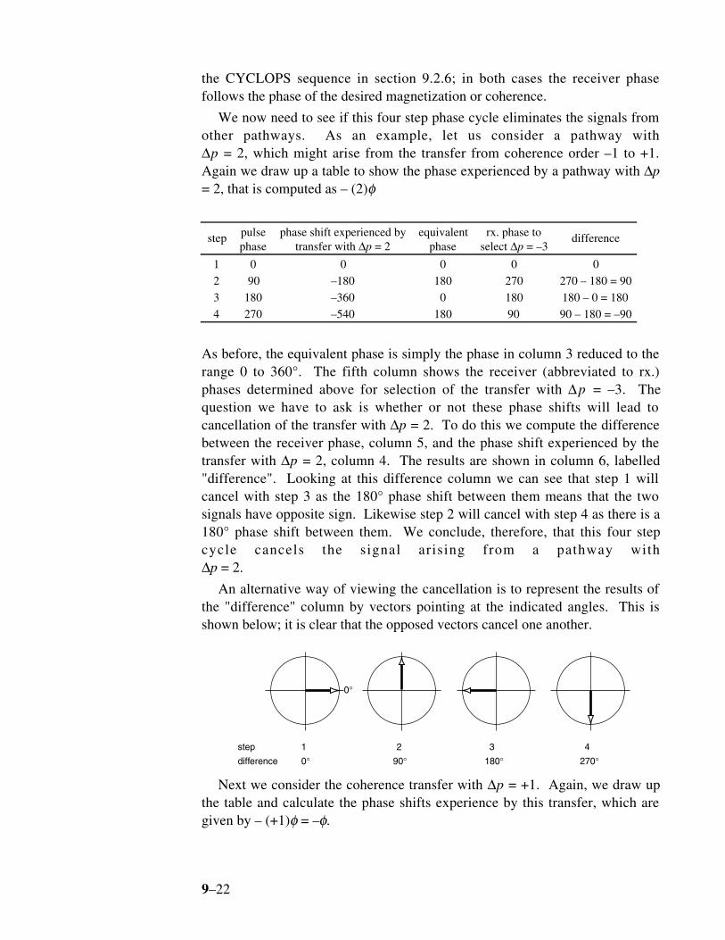
An alternative way of viewing the cancellation is to represent the results ofthe "difference" column by vectors pointing at the indicated angles. This isshown below; it is clear that the opposed vectors cancel one another.

step 1 2 3 4

difference 0°

0°

90° 180° 270°

Next we consider the coherence transfer with ∆p = +1. Again, we draw upthe table and calculate the phase shifts experience by this transfer, which aregiven by – (+1)φ = –φ.

9–23

step pulsephase

phase shift experiencedby transfer with ∆p = +1

equivalentphase

rx. phase toselect ∆p = –3

difference

1 0 0 0 0 0

2 90 –90 270 270 270 – 270 = 0

3 180 –180 180 180 180 – 180 = 0

4 270 –270 90 90 90 – 90 = 0

Here we see quite different behaviour. The equivalent phases, that is the phaseshifts experienced by the transfer with ∆p = 1, match exactly the receiverphases determined for ∆p = –3, thus the phases in the "difference" column areall zero. We conclude that the four step cycle selects transfers both with ∆p =–3 and +1.

Some more work with tables such as these will reveal that this four stepcycle suppresses contributions from changes in coherence order of –2, –1 and 0.It selects ∆p = –3 and 1. It also selects changes in coherence order of 5, 9, 13and so on. This latter sequence is easy to understand. A pathway with ∆p = 1experiences a phase shift of –90° when the pulse is shifted in phase by 90°; theequivalent phase is thus 270°. A pathway with ∆p = 5 would experience aphase shift of –5 × 90° = –450° which corresponds to an equivalent phase of270°. Thus the phase shifts experienced for ∆p = 1 and 5 are identical and it isclear that a cycle which selects one will select the other. The same goes for theseries ∆p = 9, 13 ...

The extension to negative values of ∆p is also easy to see. A pathway with∆p = –3 experiences a phase shift of 270° when the pulse is shifted in phase by90°. A transfer with ∆p = +1 experiences a phase of –90° which corresponds toan equivalent phase of 270°. Thus both pathways experience the same phaseshifts and a cycle which selects one will select the other. The pattern is clear,this four step cycle will select a pathway with ∆p = –3, as it was designed to,and also it will select any pathway with ∆p = –3 + 4n where n = ±1, ±2, ±3 ...

9.5.2 General Rules

The discussion in the previous section can be generalised in the following way.Consider a phase cycle in which the phase of a pulse takes N evenly spacedsteps covering the range 0 to 2π radians. The phases, φk, are

φk = 2πk/N where k = 0, 1, 2 ... (N – 1).

To select a change in coherence order, ∆p , the receiver phase is set to–∆p × φk for each step and the resulting signals are summed. This cycle will, inaddition to selecting the specified change in coherence order, also selectpathways with changes in coherence order (∆ p ± n N ) wheren = ±1, ±2 ..

The way in which phase cycling selects a series of values of ∆p which arerelated by a harmonic condition is closely related to the phenomenon of aliasingin Fourier transformation. Indeed, the whole process of phase cycling can be

9–24

seen as the computation of a discrete Fourier transformation with respect to thepulse phase; in this case the Fourier co-domains are phase and coherence order.

The fact that a phase cycle inevitably selects more than one change incoherence order is not necessarily a problem. We may actually wish to selectmore than one pathway, and examples of this will be given below in relation tospecific two-dimensional experiments. Even if we only require one value of ∆pwe may be able to discount the values selected at the same time as beingimprobable or insignificant. In a system of m coupled spins one-half, themaximum order of coherence that can be generated is m, thus in a two spinsystem we need not worry about whether or not a phase cycle will discriminatebetween double quantum and six quantum coherences as the latter simplycannot be present. Even in more extended spin systems the likelihood ofgenerating high-order coherences is rather small and so we may be able todiscount them for all practical purposes. If a high level of discriminationbetween orders is needed, then the solution is simply to use a phase cycle whichhas more steps i.e. in which the phases move in smaller increments. Forexample a six step cycle will discriminate between ∆p = +2 and +6, whereas afour step cycle will not.

9.5.3 Refocusing Pulses

A 180° pulse simply changes the sign of the coherence order. This is easilydemonstrated by considering the effect of such a pulse on the operators I+ andI–. For example:

I I I I I Ix yI

x yx

+ ≡ +( ) → ( ) ≡i iπ – –

corresponds to p = +1 → p = –1. In a more complex product of operators, eachraising and lowering operator is affected in this way so overall the coherenceorder changes sign.

We can now derive the EXORCYLE phase cycle using this property.Consider a 180° pulse acting on single quantum coherence, for which the CTPis shown opposite. For the pathway starting with p = 1 the effect of the 180°pulse is to cause a change with ∆p = –2. The table shows a four-step cycle toselect this change

Step phase of180° pulse

phase shift experienced bytransfer with ∆p = –2

Equivalent phase= rx. phase

1 0 0 0

2 90 180 180

3 180 360 0

4 270 540 180

The phase cycle is thus 0, 90°, 180°, 270° for the 180° pulse and0° 180° 0° 180° for the receiver; this is precisely the set of phases deducedbefore for EXORCYCLE in section 9.2.7.

10

–1

180°

A 180° pulse simply changesthe sign of the coherence order.The EXORCYLE phase cyclingselects both of the pathwaysshown.

9–25

As the cycle has four steps, a pathway with ∆p = +2 is also selected; this isthe pathway which starts with p = –1 and is transferred to p = +1. Therefore,the four steps of EXORCYLE select both of the pathways shown in the diagramabove.

A two step cycle, consisting of 0°, 180° for the 180° pulse and 0°, 0° for thereceiver, can easily be shown to select all even values of ∆p. This reduced formof EXORCYCLE is sometimes used when it is necessary to minimise thenumber of steps in a phase cycle. An eight step cycle, in which the 180° pulseis advanced in steps of 45°, can be used to select the refocusing of double-quantum coherence in which the t ransfer i s f romp = +2 to –2 (i.e. ∆p = –4) or vice versa.

9.5.4 Combining phase cycles

Suppose that we wish to select the pathway shown opposite; for the first pulse∆p is 1 and for the second it is –2. We can construct a four-step cycle for eachpulse, but to select the overall pathway shown these two cycles have to becompleted independently of one another. This means that there will be a totalof sixteen steps. The table shows how the appropriate receiver cycling can bedetermined

Step phase of 1stpulse

phase for∆p = 1

phase of 2ndpulse

phase for∆p = –2

totalphase

equivalent phase =rx. phase

1 0 0 0 0 0 0

2 90 –90 0 0 –90 270

3 180 –180 0 0 –180 180

4 270 –270 0 0 –270 90

5 0 0 90 180 180 180

6 90 –90 90 180 90 90

7 180 –180 90 180 0 0

8 270 –270 90 180 –90 270

9 0 0 180 360 360 0

10 90 –90 180 360 270 270

11 180 –180 180 360 180 180

12 270 –270 180 360 90 90

13 0 0 270 540 540 180

14 90 –90 270 540 450 90

15 180 –180 270 540 360 0

16 270 –270 270 540 270 270

In the first four steps the phase of the second pulse is held constant and thephase of the first pulse simply goes through the four steps 0° 90° 180° 270°. Aswe are selecting ∆p = 1 for this pulse, the receiver phases are simply 0°, 270°,180°, 90°.

Steps 5 to 8 are a repeat of steps 1–4 except that the phase of the secondpulse has been moved by 90°. As ∆p for the second pulse is –2, the required

10

–1

9–26

pathway experiences a phase shift of 180° and so the receiver phase must beadvanced by this much. So, the receiver phases for steps 5–8 are just 180°ahead of those for steps 1–4.

In the same way for steps 9–12 the first pulse again goes through the samefour steps, and the phase of the second pulse is advanced to 180°. Therefore,compared to steps 1–4 the receiver phases in steps 9–12 need to be advanced by– (–2) × 180° = 360° = 0°. Likewise, the receiver phases for steps 13–16 areadvanced by – (–2) × 270° = 540° = 180°.

Another way of looking at this is to consider each step individually. Forexample, compared to step 1, in step 14 the first pulse has been advanced by90° so the phase from the first pulse is – (1) × 90° = –90°. The second pulsehas been advanced by 270° so the phase from this is – (–2) × 270° = 540°. Thetotal phase shift of the required pathway is thus –90 + 540 = 450° which is anequivalent phase of 90°. This is the receiver phase shown in the final column.

The key to devising these sequences is to simply work out the two four-stepcycles independently and then merge them together rather than trying to workon the whole cycle. One writes down the first four steps, and then duplicatesthis four times as the second pulse is shifted. We would find the same steps, ina different sequence, if the phase of the second pulse is shifted in the first foursteps.

We can see that the total size of a phase cycle grows at an alarming rate.With four phases for each pulse the number of steps grows as 4l where l is thenumber of pulses in the sequence. A three-pulse sequence such as NOESY orDQF COSY would therefore involve a 64 step cycle. Such long cycles put alower limit on the total time of an experiment and we may end up having to runan experiment for a long time not to achieve the desired signal-to-noise ratiobut simply to complete the phase cycle.

Fortunately, there are several "tricks" which we can use in order to shortenthe length of a phase cycle. To appreciate whether or not one of these trickscan be used in a particular sequence we need to understand in some detail whatthe sequence is actually doing and what the likely problems are going to be.

9.5.5 Tricks

9.5.5.1 The first pulse

All pulse sequences start with equilibrium magnetization, which has coherenceorder 0. It can easily be shown that when a pulse is applied to equilibriummagnetization the only coherence orders that can be generated are ±1. Ifretaining both of these orders is acceptable (which it often is), it is therefore notnecessary to phase cycle the first pulse in a sequence.

There are two additional points to make here. If the spins have not relaxedcompletely by the start of the sequence the initial magnetization will not be atequilibrium. Then, the above simplification does not apply. Secondly, the firstpulse of a sequence is often cycled in order to suppress axial peaks in two-

9–27

dimensional spectra. This is considered in more detail in section 9.5.6.

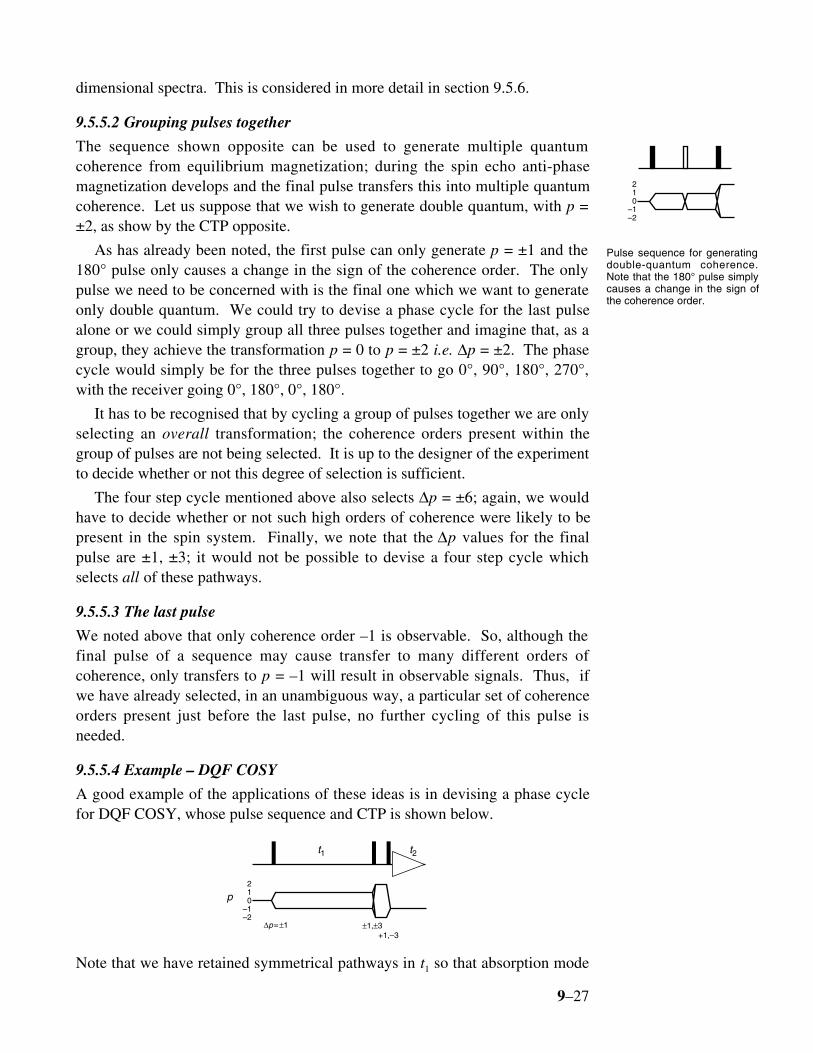
9.5.5.2 Grouping pulses together

The sequence shown opposite can be used to generate multiple quantumcoherence from equilibrium magnetization; during the spin echo anti-phasemagnetization develops and the final pulse transfers this into multiple quantumcoherence. Let us suppose that we wish to generate double quantum, with p =±2, as show by the CTP opposite.

As has already been noted, the first pulse can only generate p = ±1 and the180° pulse only causes a change in the sign of the coherence order. The onlypulse we need to be concerned with is the final one which we want to generateonly double quantum. We could try to devise a phase cycle for the last pulsealone or we could simply group all three pulses together and imagine that, as agroup, they achieve the transformation p = 0 to p = ±2 i.e. ∆p = ±2. The phasecycle would simply be for the three pulses together to go 0°, 90°, 180°, 270°,with the receiver going 0°, 180°, 0°, 180°.

It has to be recognised that by cycling a group of pulses together we are onlyselecting an overall transformation; the coherence orders present within thegroup of pulses are not being selected. It is up to the designer of the experimentto decide whether or not this degree of selection is sufficient.

The four step cycle mentioned above also selects ∆p = ±6; again, we wouldhave to decide whether or not such high orders of coherence were likely to bepresent in the spin system. Finally, we note that the ∆p values for the finalpulse are ±1, ±3; it would not be possible to devise a four step cycle whichselects all of these pathways.

9.5.5.3 The last pulse

We noted above that only coherence order –1 is observable. So, although thefinal pulse of a sequence may cause transfer to many different orders ofcoherence, only transfers to p = –1 will result in observable signals. Thus, ifwe have already selected, in an unambiguous way, a particular set of coherenceorders present just before the last pulse, no further cycling of this pulse isneeded.

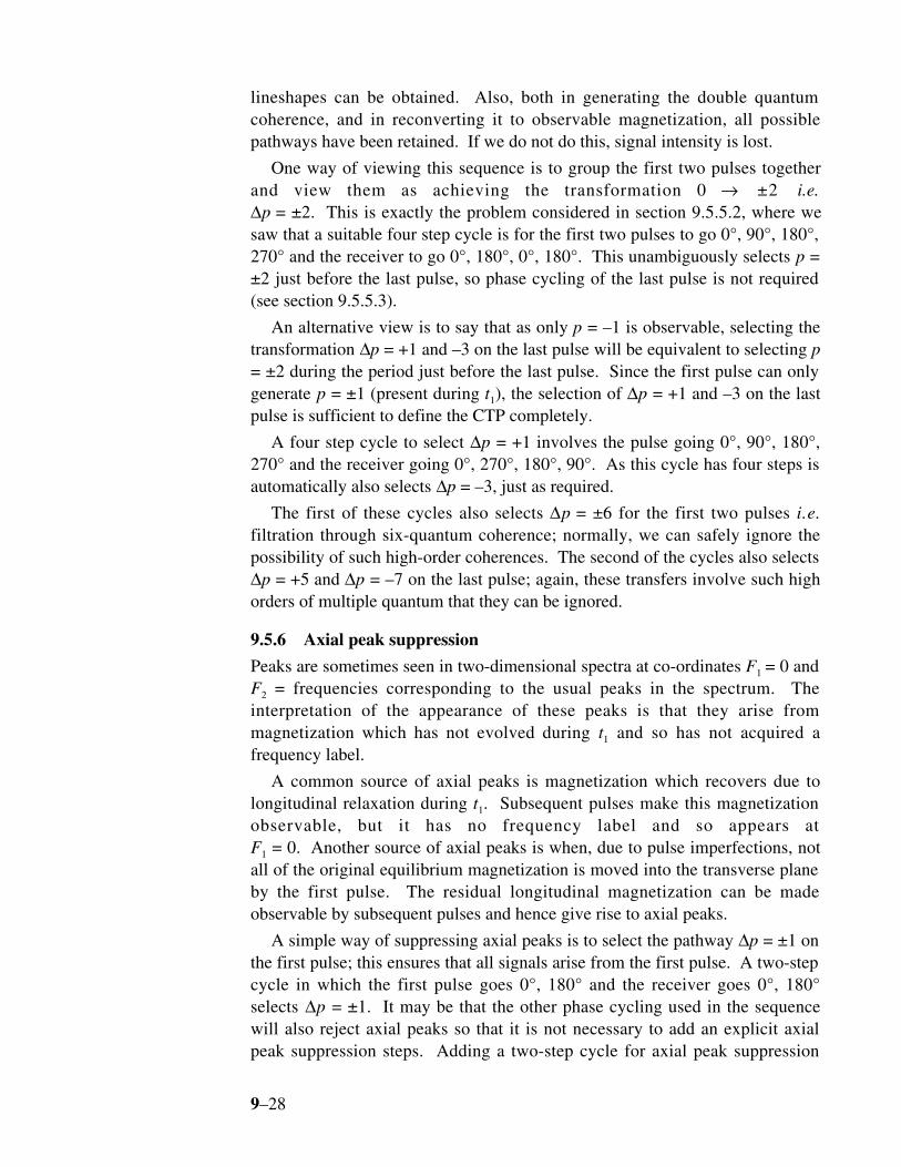
9.5.5.4 Example – DQF COSY

A good example of the applications of these ideas is in devising a phase cyclefor DQF COSY, whose pulse sequence and CTP is shown below.

t1 t2

210

–1–2

p

∆p=±1 ±1,±3+1,–3

Note that we have retained symmetrical pathways in t1 so that absorption mode

210

–1–2

Pulse sequence for generatingdouble-quantum coherence.Note that the 180° pulse simplycauses a change in the sign ofthe coherence order.

9–28

lineshapes can be obtained. Also, both in generating the double quantumcoherence, and in reconverting it to observable magnetization, all possiblepathways have been retained. If we do not do this, signal intensity is lost.

One way of viewing this sequence is to group the first two pulses togetherand view them as achieving the transformation 0 → ±2 i.e.∆p = ±2. This is exactly the problem considered in section 9.5.5.2, where wesaw that a suitable four step cycle is for the first two pulses to go 0°, 90°, 180°,270° and the receiver to go 0°, 180°, 0°, 180°. This unambiguously selects p =±2 just before the last pulse, so phase cycling of the last pulse is not required(see section 9.5.5.3).

An alternative view is to say that as only p = –1 is observable, selecting thetransformation ∆p = +1 and –3 on the last pulse will be equivalent to selecting p= ±2 during the period just before the last pulse. Since the first pulse can onlygenerate p = ±1 (present during t1), the selection of ∆p = +1 and –3 on the lastpulse is sufficient to define the CTP completely.

A four step cycle to select ∆p = +1 involves the pulse going 0°, 90°, 180°,270° and the receiver going 0°, 270°, 180°, 90°. As this cycle has four steps isautomatically also selects ∆p = –3, just as required.

The first of these cycles also selects ∆p = ±6 for the first two pulses i.e.filtration through six-quantum coherence; normally, we can safely ignore thepossibility of such high-order coherences. The second of the cycles also selects∆p = +5 and ∆p = –7 on the last pulse; again, these transfers involve such highorders of multiple quantum that they can be ignored.

9.5.6 Axial peak suppression

Peaks are sometimes seen in two-dimensional spectra at co-ordinates F1 = 0 andF2 = frequencies corresponding to the usual peaks in the spectrum. Theinterpretation of the appearance of these peaks is that they arise frommagnetization which has not evolved during t1 and so has not acquired afrequency label.

A common source of axial peaks is magnetization which recovers due tolongitudinal relaxation during t1. Subsequent pulses make this magnetizationobservable, but it has no frequency label and so appears atF1 = 0. Another source of axial peaks is when, due to pulse imperfections, notall of the original equilibrium magnetization is moved into the transverse planeby the first pulse. The residual longitudinal magnetization can be madeobservable by subsequent pulses and hence give rise to axial peaks.

A simple way of suppressing axial peaks is to select the pathway ∆p = ±1 onthe first pulse; this ensures that all signals arise from the first pulse. A two-stepcycle in which the first pulse goes 0°, 180° and the receiver goes 0°, 180°selects ∆p = ±1. It may be that the other phase cycling used in the sequencewill also reject axial peaks so that it is not necessary to add an explicit axialpeak suppression steps. Adding a two-step cycle for axial peak suppression

9–29

doubles the length of the phase cycle.

9.5.7 Shifting the whole sequence – CYCLOPS

If we group all of the pulses in the sequence together and regard them as a unitthey simply achieve the transformation from equilibrium magnetization, p = 0,to observable magnetization, p = –1. They could be cycled as a group to selectthis pathway with ∆p = –1, that is the pulses going 0°, 90°, 180°, 270° and thereceiver going 0°, 90°, 180°, 270°. This is simple the CYCLOPS phase cycledescribed in section 9.2.6.

If time permits we sometimes add CYCLOPS-style cycling to all of thepulses in the sequence so as to suppress some artefacts associated withimperfections in the receiver. Adding such cycling does, of course, extend thephase cycle by a factor of four.

This view of the whole sequence as causing the transformation ∆p = –1 alsoenables us to interchange receiver and pulse phase shifts. For example, supposethat a particular step in a phase cycle requires a receiver phase shift θ. Thesame effect can be achieved by shifting all of the pulses by –θ and leaving thereceiver phase unaltered. The reason this works is that all of the pulses takentogether achieve the transformation ∆p = –1, so shifting their phases by –θ shiftthe signal by – (–θ) = θ, which is exactly the effect of shifting the receiver by θ.This kind of approach is sometimes helpful if hardware limitations mean thatsmall angle phase-shifts are only available for the pulses.

9.5.8 Equivalent cycles

For even a relatively simple sequence such as DQF COSY there are a numberof different ways of writing the phase cycle. Superficially these can look verydifferent, but it may be possible to show that they really are the same.

For example, consider the DQF COSY phase cycle proposed in section9.5.5.4 where we cycle just the last pulse

step 1st pulse 2nd pulse 3rd pulse receiver

1 0 0 0 0

2 0 0 90 270

3 0 0 180 180

4 0 0 270 90

Suppose we decide that we do not want to shift the receiver phase, but want tokeep it fixed at phase zero. As described above, this means that we need tosubtract the receiver phase from all of the pulses. So, for example, in step 2 wesubtract 270° from the pulse phases to give –270°, –270° and –180° for thephases of the first three pulses, respectively; reducing these to the usual rangegives phases 90°, 90° and 180°. Doing the same for the other steps gives arather strange looking phase cycle, but one which works in just the same way.

step 1st pulse 2nd pulse 3rd pulse receiver

9–30

1 0 0 0 0

2 90 90 180 0

3 180 180 0 0

4 270 270 180 0

We can play one more trick with this phase cycle. As the third pulse is requiredto achieve the transformation ∆p = –3 or +1 we can alter its phase by 180° andcompensate for this by shifting the receiver by 180° also. Doing this for steps 2and 4 only gives

step 1st pulse 2nd pulse 3rd pulse receiver

1 0 0 0 0

2 90 90 0 180

3 180 180 0 0

4 270 270 0 180

This is exactly the cycle proposed in section 9.5.5.4.

9.5.9 Further examples

In this section we will use a shorthand to indicate the phases of the pulses andthe receiver. Rather than specifying the phase in degrees, the phases areexpressed as multiples of 90°. So, EXORCYCLE becomes 0 1 2 3 for the180° pulse and 0 2 0 2 for the receiver.

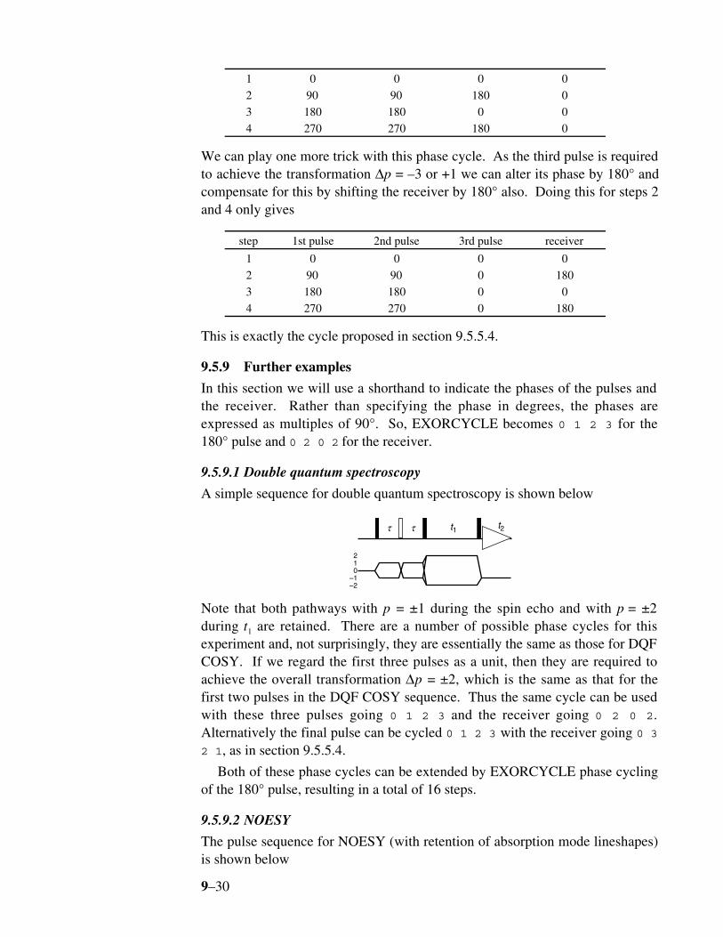
9.5.9.1 Double quantum spectroscopy

A simple sequence for double quantum spectroscopy is shown below

t1 t2

210

–1–2

τ τ

Note that both pathways with p = ±1 during the spin echo and with p = ±2during t1 are retained. There are a number of possible phase cycles for thisexperiment and, not surprisingly, they are essentially the same as those for DQFCOSY. If we regard the first three pulses as a unit, then they are required toachieve the overall transformation ∆p = ±2, which is the same as that for thefirst two pulses in the DQF COSY sequence. Thus the same cycle can be usedwith these three pulses going 0 1 2 3 and the receiver going 0 2 0 2.Alternatively the final pulse can be cycled 0 1 2 3 with the receiver going 0 32 1, as in section 9.5.5.4.

Both of these phase cycles can be extended by EXORCYCLE phase cyclingof the 180° pulse, resulting in a total of 16 steps.

9.5.9.2 NOESY

The pulse sequence for NOESY (with retention of absorption mode lineshapes)is shown below

9–31

t1 t2

10

–1

τmix

If we group the first two pulses together they are required to achieve thetransformation ∆p = 0 and this leads to a four step cycle in which the pulses go0 1 2 3 and the receiver remains fixed as 0 0 0 0. In this experiment axialpeaks arise due to z-magnetization recovering during the mixing time, and thiscycle will not suppress these contributions. Thus we need to add axial peaksuppression, which is conveniently done by adding the simple cycle 0 2 on thefirst pulse and the receiver. The final 8 step cycle is 1st pulse: 0 1 2 3 2 30 1, 2nd pulse: 0 1 2 3 0 1 2 3, 3rd pulse fixed, receiver: 0 0 0 0 2 22 2.

An alternative is to cycle the last pulse to select the pathway ∆p = –1, givingthe cycle 0 1 2 3 for the pulse and 0 1 2 3 for the receiver. Once again, thisdoes not discriminate against z-magnetization which recovers during the mixingtime, so a two step phase cycle to select axial peaks needs to be added.

9.5.9.3 Heteronuclear Experiments

The phase cycling for most heteronuclear experiments tends to be rather trivialin that the usual requirement is simply to select that component which has beentransferred from one nucleus to another. We have already seen in section 9.2.8that this is achieved by a 0 2 phase cycle on one of the pulses causing thetransfer accompanied by the same on the receiver i.e. a difference experiment.The choice of which pulse to cycle depends more on practical considerationsthan with any fundamental theoretical considerations.

The pulse sequence for HMQC, along with the CTP, is shown below

t2

10

–1

t1

10

–1

∆ ∆I

S

pI

pS

Note that separate coherence orders are assigned to the I and S spins.Observable signals on the I spin must have pI = –1 and pS = 0 (any other valueof pS would correspond to a heteronuclear multiple quantum coherence). Giventhis constraint, and the fact that the I spin 180° pulse simply inverts the sign ofpI, the only possible pathway on the I spins is that shown.

The S spin coherence order only changes when pulses are applied to thosespins. The first 90° S spin pulse generates pS = ±1, just as before. As by thispoint pI = +1, the resulting coherences have pS = +1, pI = –1 (heteronuclearzero-quantum) and pS = +1, pI = +1 (heteronuclear double-quantum). The I spin

9–32

180° pulse interconverts these midway during t1, and finally the last S spinpulse returns both pathways to pS = 0. A detailed analysis of the sequenceshows that retention of both of these pathways results in amplitude modulationin t1 (provided that homonuclear couplings between I spins are not resolved inthe F1 dimension).

Usually, the I spins are protons and the S spins some low-abundanceheteronucleus, such as 13C. The key thing that we need to achieve is to suppressthe signals arising from vast majority of I spins which are not coupled to Sspins. This is achieved by cycling a pulse which affects the phase of therequired coherence but which does not affect that of the unwanted coherence.The obvious targets are the two S spin 90° pulses, each of which is required togive the transformation ∆pS = ±1. A two step cycle with either of these pulsesgoing 0 2 and the receiver doing the same will select this pathway and, bydifference, suppress any I spin magnetization which has not been passed intomultiple quantum coherence.

It is also common to add EXORCYCLE phase cycling to the I spin 180°pulse, giving a cycle with eight steps overall.

9.5.10 General points about phase cycling

Phase cycling as a method suffers from two major practical problems. The firstis that the need to complete the cycle imposes a minimum time on theexperiment. In two- and higher-dimensional experiments this minimum timecan become excessively long, far longer than would be needed to achieve thedesired signal-to-noise ratio. In such cases the only way of reducing theexperiment time is to record fewer increments which has the undesirableconsequence of reducing the limiting resolution in the indirect dimensions.

The second problem is that phase cycling always relies on recording allpossible contributions and then cancelling out the unwanted ones by combiningsubsequent signals. If the spectrum has high dynamic range, or if spectrometerstability is a problem, this cancellation is less than perfect. The result isunwanted peaks and t1-noise appearing in the spectrum. These problemsbecome acute when dealing with proton detected heteronuclear experiments onnatural abundance samples, or in trying to record spectra with intense solventresonances.

Both of these problems are alleviated to a large extent by moving to analternative method of selection, the use of field gradient pulses, which is thesubject of the next section. However, as we shall see, this alternative method isnot without its own difficulties.

9.6 Selection with field gradient pulses

9.6.1 Introduction

Like phase cycling, field gradient pulses can be used to select particularcoherence transfer pathways. During a pulsed field gradient the applied

9–33

magnetic field is made spatially inhomogeneous for a short time. As a result,transverse magnetization and other coherences dephase across the sample andare apparently lost. However, this loss can be reversed by the application of asubsequent gradient which undoes the dephasing process and thus restores themagnetization or coherence. The crucial property of the dephasing process isthat it proceeds at a different rate for different coherences. For example,double-quantum coherence dephases twice as fast as single-quantum coherence.Thus, by applying gradient pulses of different strengths or durations it ispossible to refocus coherences which have, for example, been changed fromsingle- to double-quantum by a radiofrequency pulse.

Gradient pulses are introduced into the pulse sequence in such a way thatonly the wanted signals are observed in each experiment. Thus, in contrast tophase cycling, there is no reliance on subtraction of unwanted signals, and itcan thus be expected that the level of t1-noise will be much reduced. Again incontrast to phase cycling, no repetitions of the experiment are needed, enablingthe overall duration of the experiment to be set strictly in accord with therequired resolution and signal-to-noise ratio.

The properties of gradient pulses and the way in which they can be used toselect coherence transfer pathways have been known since the earliest days ofmultiple-pulse NMR. However, in the past their wide application has beenlimited by technical problems which made it difficult to use such pulses inhigh-resolution NMR. The problem is that switching on the gradient pulseinduces currents in any nearby conductors, such as the probe housing andmagnet bore tube. These induced currents, called eddy currents, themselvesgenerate magnetic fields which perturb the NMR spectrum. Typically, the eddycurrents are large enough to disrupt severely the spectrum and can last manyhundreds of milliseconds. It is thus impossible to observe a high-resolutionspectrum immediately after the application of a gradient pulse. Similarproblems have beset NMR imaging experiments and have led to thedevelopment of shielded gradient coils which do not produce significantmagnetic fields outside the sample volume and thus minimise the generation ofeddy currents. The use of this technology in high-resolution NMR probes hasmade it possible to observe spectra within tens of microseconds of applying agradient pulse. With such apparatus, the use of field gradient pulses in highresolution NMR is quite straightforward, a fact first realised and demonstratedby Hurd whose work has pioneered this whole area.

9.6.2 Dephasing caused by gradients

A field gradient pulse is a period during which the B0 field is made spatiallyinhomogeneous; for example an extra coil can be introduced into the sampleprobe and a current passed through the coil in order to produce a field whichvaries linearly in the z-direction. We can imagine the sample being divided intothin discs which, as a consequence of the gradient, all experience differentmagnetic fields and thus have different Larmor frequencies. At the beginning

9–34

of the gradient pulse the vectors representing transverse magnetization in allthese discs are aligned, but after some time each vector has precessed through adifferent angle because of the variation in Larmor frequency. After sufficienttime the vectors are disposed in such a way that the net magnetization of thesample (obtained by adding together all the vectors) is zero. The gradient pulseis said to have dephased the magnetization.

It is most convenient to view this dephasing process as being due to thegeneration by the gradient pulse of a spatially dependent phase. Suppose thatthe magnetic field produced by the gradient pulse, Bg, varies linearly along thez-axis according to

B Gzg =

where G is the gradient strength expressed in, for example, T m–1 or G cm–1; theorigin of the z-axis is taken to be in the centre of the sample. At any particularposition in the sample the Larmor frequency, ωL(z), depends on the appliedmagnetic field, B0, and Bg

ω γ γL 0 g 0= +( ) = +( )B B B Gz ,

where γ is the gyromagnetic ratio. After the gradient has been applied for timet, the phase at any position in the sample, Φ(z), is given by Φ z B Gz t( ) = +( )γ 0 .The first part of this phase is just that due to the usual Larmor precession in theabsence of a field gradient. Since this is constant across the sample it will beignored from now on (which is formally the same result as viewing themagnetization in a frame of reference rotating at γB0). The remaining term γGztis the spatially dependent phase induced by the gradient pulse.

If a gradient pulse is applied to pure x-magnetization, the followingevolution takes place at a particular position in the sample

I Gzt I Gzt IxGztI

x yzγ γ γ → ( ) + ( )cos sin .

The total x-magnetization in the sample, Mx, is found by adding up themagnetization from each of the thin discs, which is equivalent to the integral

Mx t( ) = 1rmax

cos γGzt( ) dz– 1

2 rmax

12 rmax

∫

where it has been assumed that the sample extends over a region ± 12 rmax .

Evaluating the integral gives an expression for the decay of x-magnetizationduring a gradient pulse

M tGr t

Gr tx ( ) = ( )sin 12

12

γγ

max

max

[11]

The plot below shows Mx(t) as a function of time

9–35

10 20 30 40 50

-0.5

0.0

0.5

1.0

Mx

Grmaxtγ

The black line shows the decay of magnetization due to the action of a gradient pulse. The grey line is anapproximation, valid at long times, for the envelope of the decay.

Note that the oscillations in the decaying magnetization are imposed on anoverall decay which, for long times, is given by 2/(γGtrmax). Equation [11]embodies the obvious points that the stronger the gradient (the larger G) thefaster the magnetization decays and that magnetization from nuclei with highergyromagnetic ratios decays faster. It also allows a quantitative assessment ofthe gradient strengths required: the magnetization will have decayed to afraction α of its initial value after a time of the order of 2 γ αG rmax( ) (therelation is strictly valid for α << 1). For example, if it is assumed that rmax is 1cm, then a 2 ms gradient pulse of strength 0.37 T m–1 (37 G cm–1) will reduceproton magnetization by a factor of 1000. Gradients of such strength arereadily obtainable using modern shielded gradient coils that can be built intohigh resolution NMR probes

This discussion now needs to be generalised for the case of a field gradientpulse whose amplitude is not constant in time, and for the case of dephasing ageneral coherence of order p. The former modification is of importance as forinstrumental reasons the amplitude envelope of the gradient is often shaped to asmooth function. In general after applying a gradient pulse of duration τ thespatially dependent phase, Φ(r,τ) is given by

Φ r sp B r,τ γ τ( ) = ( )g [12]

The proportionality to the coherence order comes about due to the fact that thephase acquired as a result of a z-rotation of a coherence of order p through anangle φ is pφ, (see Eqn. [2] in section 9.3.1). In Eqn. [12] s is a shape factor: ifthe envelope of the gradient pulse is defined by the function A(t), whereA t( ) ≤ 1, s is defined as the area under A(t)

s A t t= ( )∫1

0τ

τ

d

The shape factor takes a particular value for a certain shape of gradient,regardless of its duration. A gradient applied in the opposite sense, that is withthe magnetic field decreasing as the z-coordinate increases rather than vice

9–36

versa, is described by reversing the sign of s. The overall amplitude of thegradient is encoded within Bg.

In the case that the coherence involves more than one nuclear species, Eqn.[12] is modified to take account of the different gyromagnetic ratio for eachspin, γi, and the (possibly) different order of coherence with respect to eachnuclear species, pi:

Φ r sB r pi ii

,τ τ γ( ) = ( ) ∑g

From now on we take the dependence of Φ on r and τ, and of Bg on r as beingimplicit.

9.6.3 Selection by refocusing

The method by which a particular coherence transfer pathway is selected usingfield gradients is illustrated opposite. The first gradient pulse encodes aspatially dependent phase, Φ1 and the second a phase Φ2 where

Φ Φ1 1 1 1 2 2 2 2= =s p B s p Bγ τ γ τg,1 g,2and .

After the second gradient the net phase is (Φ1 + Φ2). To select the pathwayinvolving transfer from coherence order p1 to coherence order p2, this net phaseshould be zero; in other words the dephasing induced by the first gradient pulseis undone by the second. The condition (Φ1 + Φ2) = 0 can be rearranged to

s B

s B

p

p1 1

2 2

2

1

g,1

g,2

ττ

= –

. [13]

For example, if p1 = +2 and p2 = –1, refocusing can be achieved by making thesecond gradient either twice as long (τ 2 = 2τ1), or twice as strong(Bg,2 = 2Bg,1) as the first; this assumes that the two gradients have identicalshape factors. Other pathways remain dephased; for example, assuming that wehave chosen to make the second gradient twice as strong and the same durationas the first, a pathway with p1 = +3 to p2 = –1 experiences a net phase

Φ Φ1 2 1 1 13+ = =sB sB sBg,1 g,2 g,1τ τ τ– .

Provided that this spatially dependent phase is sufficiently large, according thecriteria set out in the previous section, the coherence arising from this pathwayremains dephased and is not observed. To refocus a pathway in which there isno sign change in the coherence orders, for example, p1 = –2 to p2 = –1, thesecond gradient needs to be applied in the opposite sense to the first; in terms ofEqn. [13] this is expressed by having s2 = –s1.

The procedure can easily be extended to select a more complex coherencetransfer pathway by applying further gradient pulses as the coherence istransferred by further pulses, as illustrated opposite. The condition forrefocusing is again that the net phase acquired by the required pathway be zero,which can be written formally as

p1

p2

RF

g1τ 2τ

Illustration of the use of a pairof gradients to select a singlepathway. The radiofrequencypulses are on the line marked"RF" and the field gradientpulses are denoted by shadedrectangles on the line marked"g".

RF

g1τ 3τ 4τ2τ

9–37

s p Bi i i ii

γ τg,i∑ = 0 .

With more than two gradients in the sequence, there are many ways in which agiven pathway can be selected. For example, the second gradient may be usedto refocus the first part of the required pathway, leaving the third and fourth torefocus another part. Alternatively, the pathway may be consistently dephasedand the magnetization only refocused by the final gradient, just beforeacquisition.

At this point it is useful to contrast the selection achieved using gradientpulses with that achieved using phase cycling. From Eqn. [13] it is clear that aparticular pair of gradient pulses selects a particular ratio of coherence orders;in the above example any two coherence orders in the ratio –2 : 1 or 2 : –1 willbe refocused. This selection according to ratio of coherence orders is incontrast to the case of phase cycling in which a phase cycle consisting of Nsteps of 2π/N radians selects a particular change in coherence order ∆p = p2 –p1, and further pathways which have ∆p = (p2 – p1) ± mN, where m = 0, 1, 2 ...

It is straightforward to devise a series of gradient pulses which will select asingle coherence transfer pathway. It cannot be assumed, however, that such asequence of gradient pulses will reject all other pathways i.e. leave coherencefrom all other pathways dephased at the end of the sequence. Such assurancecan only be given be analysing the fate of all other possible coherence transferpathways under the particular gradient sequence proposed. In complex pulsesequences there may also be several different ways in which gradient pulses canbe included in order to achieve selection of the desired pathway. Assessingwhich of these alternatives is the best, in the light of the requirement ofsuppression of unwanted pathways and the effects of pulse imperfections maybe a complex task.

9.6.3.1 Selection of multiple pathways

As we have seen earlier, it is not unusual to want to select two or morepathways simultaneously, for example either to maximise the signal intensity orto retain absorption-mode lineshapes. A good example of this is the double-quantum filter pulse sequence element, shown opposite.

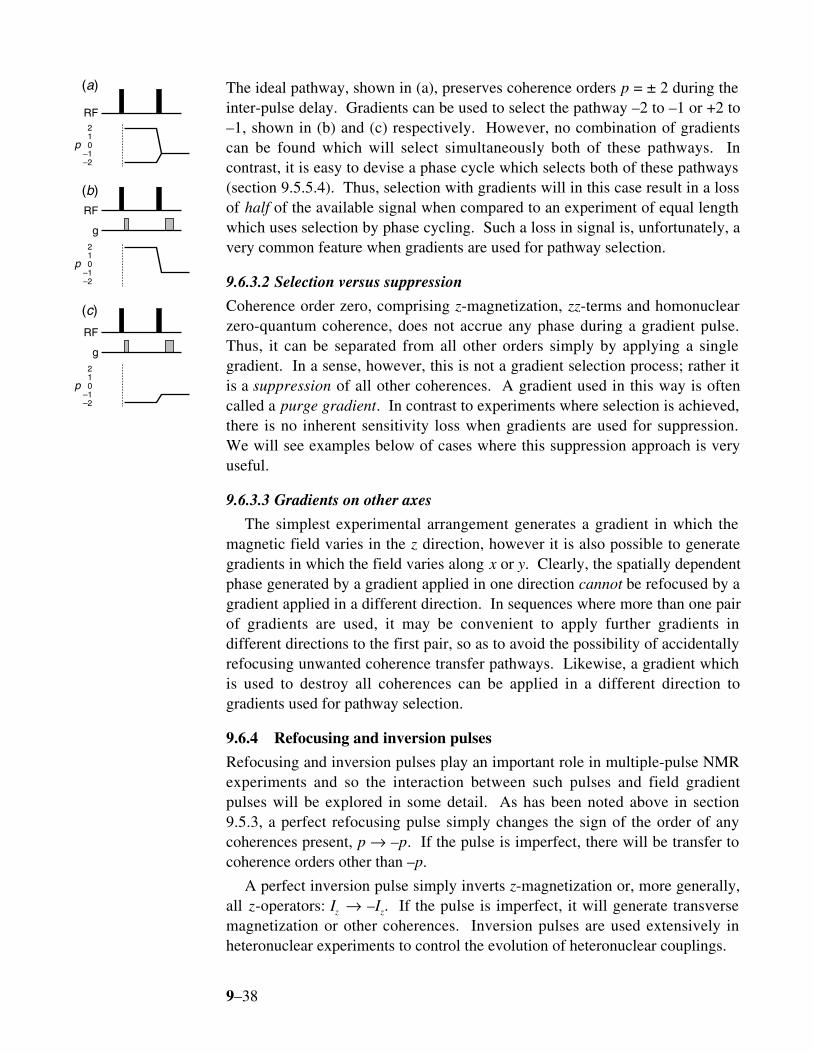
9–38

The ideal pathway, shown in (a), preserves coherence orders p = ± 2 during theinter-pulse delay. Gradients can be used to select the pathway –2 to –1 or +2 to–1, shown in (b) and (c) respectively. However, no combination of gradientscan be found which will select simultaneously both of these pathways. Incontrast, it is easy to devise a phase cycle which selects both of these pathways(section 9.5.5.4). Thus, selection with gradients will in this case result in a lossof half of the available signal when compared to an experiment of equal lengthwhich uses selection by phase cycling. Such a loss in signal is, unfortunately, avery common feature when gradients are used for pathway selection.

9.6.3.2 Selection versus suppression

Coherence order zero, comprising z-magnetization, zz-terms and homonuclearzero-quantum coherence, does not accrue any phase during a gradient pulse.Thus, it can be separated from all other orders simply by applying a singlegradient. In a sense, however, this is not a gradient selection process; rather itis a suppression of all other coherences. A gradient used in this way is oftencalled a purge gradient. In contrast to experiments where selection is achieved,there is no inherent sensitivity loss when gradients are used for suppression.We will see examples below of cases where this suppression approach is veryuseful.

9.6.3.3 Gradients on other axes

The simplest experimental arrangement generates a gradient in which themagnetic field varies in the z direction, however it is also possible to generategradients in which the field varies along x or y. Clearly, the spatially dependentphase generated by a gradient applied in one direction cannot be refocused by agradient applied in a different direction. In sequences where more than one pairof gradients are used, it may be convenient to apply further gradients indifferent directions to the first pair, so as to avoid the possibility of accidentallyrefocusing unwanted coherence transfer pathways. Likewise, a gradient whichis used to destroy all coherences can be applied in a different direction togradients used for pathway selection.

9.6.4 Refocusing and inversion pulses

Refocusing and inversion pulses play an important role in multiple-pulse NMRexperiments and so the interaction between such pulses and field gradientpulses will be explored in some detail. As has been noted above in section9.5.3, a perfect refocusing pulse simply changes the sign of the order of anycoherences present, p → –p. If the pulse is imperfect, there will be transfer tocoherence orders other than –p.

A perfect inversion pulse simply inverts z-magnetization or, more generally,all z-operators: Iz → –Iz. If the pulse is imperfect, it will generate transversemagnetization or other coherences. Inversion pulses are used extensively inheteronuclear experiments to control the evolution of heteronuclear couplings.

RF

g

210

–1–2

p

RF

210

–1–2

p

g

RF

210

–1–2

p

(a)

(b)

(c)

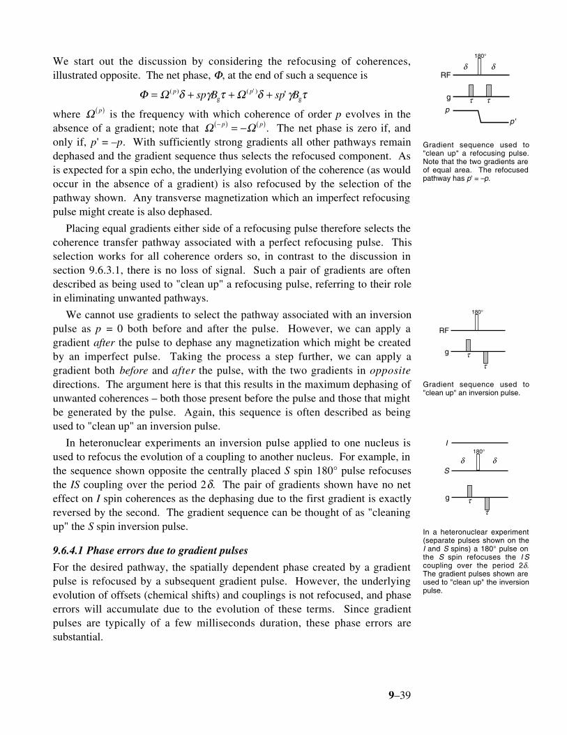
9–39

We start out the discussion by considering the refocusing of coherences,illustrated opposite. The net phase, Φ, at the end of such a sequence is

Φ Ω Ω= + + +( ) ( ' ) 'p psp B sp Bδ γ τ δ γ τg g

where Ω p( ) is the frequency with which coherence of order p evolves in theabsence of a gradient; note that Ω Ω−( ) ( )= −p p . The net phase is zero if, andonly if, p' = –p. With sufficiently strong gradients all other pathways remaindephased and the gradient sequence thus selects the refocused component. Asis expected for a spin echo, the underlying evolution of the coherence (as wouldoccur in the absence of a gradient) is also refocused by the selection of thepathway shown. Any transverse magnetization which an imperfect refocusingpulse might create is also dephased.

Placing equal gradients either side of a refocusing pulse therefore selects thecoherence transfer pathway associated with a perfect refocusing pulse. Thisselection works for all coherence orders so, in contrast to the discussion insection 9.6.3.1, there is no loss of signal. Such a pair of gradients are oftendescribed as being used to "clean up" a refocusing pulse, referring to their rolein eliminating unwanted pathways.

We cannot use gradients to select the pathway associated with an inversionpulse as p = 0 both before and after the pulse. However, we can apply agradient after the pulse to dephase any magnetization which might be createdby an imperfect pulse. Taking the process a step further, we can apply agradient both before and after the pulse, with the two gradients in oppositedirections. The argument here is that this results in the maximum dephasing ofunwanted coherences – both those present before the pulse and those that mightbe generated by the pulse. Again, this sequence is often described as beingused to "clean up" an inversion pulse.

In heteronuclear experiments an inversion pulse applied to one nucleus isused to refocus the evolution of a coupling to another nucleus. For example, inthe sequence shown opposite the centrally placed S spin 180° pulse refocusesthe IS coupling over the period 2δ. The pair of gradients shown have no neteffect on I spin coherences as the dephasing due to the first gradient is exactlyreversed by the second. The gradient sequence can be thought of as "cleaningup" the S spin inversion pulse.

9.6.4.1 Phase errors due to gradient pulses

For the desired pathway, the spatially dependent phase created by a gradientpulse is refocused by a subsequent gradient pulse. However, the underlyingevolution of offsets (chemical shifts) and couplings is not refocused, and phaseerrors will accumulate due to the evolution of these terms. Since gradientpulses are typically of a few milliseconds duration, these phase errors aresubstantial.

p

p'

RF

g τ τ

180°

δ δ

Gradient sequence used to"clean up" a refocusing pulse.Note that the two gradients areof equal area. The refocusedpathway has p' = –p.

RF

g ττ

180°

Gradient sequence used to"clean up" an inversion pulse.

I

S

g τ

δ δ

τ

180°

In a heteronuclear experiment(separate pulses shown on theI and S spins) a 180° pulse onthe S spin refocuses the I Scoupling over the period 2δ.The gradient pulses shown areused to "clean up" the inversionpulse.

9–40

In multi-dimensional NMR the uncompensated evolution of offsets duringgradient pulses has disastrous effects on the spectra. This is illustrated here forthe DQF COSY experiment, for which a pulse sequence using the gradientpulses is shown opposite. The problem with this sequence is that the doublequantum coherence will evolve during delay τ1. Normally, the delay betweenthe last two pulses would be a few microseconds at most, during which theevolution is negligible. However, once we need to apply a gradient the delaywill need to be of the order of milliseconds and significant evolution takesplace. The same considerations apply to the second gradient.

We can investigate the effect of this evolution by analysing the result for atwo-spin system. In the calculation, it will be assumed that only the indicatedpathway survives and that the spatially dependent part of the evolution due tothe gradients can be ignored as ultimately it is refocused. The coherence withorder of + 2 present during τ1 evolves according to

I I I I iI Iz z

1 2 1 2 1 2 11 1 1 2 1 2

+ ++

+ + → +( )( )Ω Ω Ω Ωτ τ τexp – ,

where Ω1 and Ω2 are the offsets of spins 1 and 2, respectively. After the final90° pulse and the second gradient the observable terms on spin 1 are

i2 1 2 1 1 2 1 2 1 2 1 22 2exp – cos sini I I I Ix z y zΩ Ω Ω Ω+( )( ) +[ ]τ τ τ [14]

where it has been assumed that τ2 is sufficiently short that evolution of thecoupling can be ignored. It is clearly seen from Eqn. [14] that, due to theevolution during τ2, the multiplet observed in the F2 dimension will be amixture of dispersion and absorption anti-phase contributions. In addition,there is an overall phase shift due to the evolution during τ1. The phasecorrection needed to restore this multiplet to absorption depends on both thefrequency in F2 and the double-quantum frequency during the first gradient.Thus, no single linear frequency dependent phase correction could phasecorrect a spectrum containing many multiplets. The need to control these phaseerrors is plain.

The general way to minimise these problems is to associate each gradientwith a refocusing pulse, as shown opposite. In sequence (a) the gradient isplaced in one of the delays of a spin echo; the evolution of the offset during thefirst delay τ is refocused during the second delay τ. So, overall there are nophase errors due to the evolution of the offset.

An alternative is the sequence (b). Here, as in (a), the offset is refocusedover the whole sequence. The first gradient results in the usually spatiallydependent phase and then the 180° pulse changes the sign of the coherenceorder. As the second gradient is opposite to the first, it causes furtherdephasing; effectively, it is as if a gradient of length 2τ is applied. Sequence(b) will give the same dephasing effect as (a) if each gradient in (b) is ofduration τ/2; the overall sequence will then be of duration τ. If losses due torelaxation are a problem, then clearly sequence (b) is to be preferred as it takesless time than (a).

g

RF

210

–1–2

t1 t2

1τ 2τ

Simple pulse sequence forDQF COSY with gradientselection and retention ofsymmetrical pathways in t1.The second gradient is twicethe area of the first.

RF

180°

g τ

τ τ(a)

(b)

RF

180°

g ττ

τ τ

9–41

The sequence below shows the gradient-selected DQF COSY pulse sequencemodified by the inclusion of extra 180° pulses to remove phase errors. Notethat although the extra 180° pulses are effective at refocusing offsets, they donot refocus the evolution of homonuclear couplings. It is essential, therefore, tokeep the gradient pulses as short as is feasible.

g

RFt1

1τ

1τ 1τ

2τ

2τ 2τ

In many pulse sequences there are already periods during which theevolution of offsets is refocused. The evolution of offsets during a gradientpulse placed within such a period will therefore also be refocused, making itunnecessary to include extra refocusing pulses. Likewise, a gradient may beplaced during a "constant time" evolution period of a multi-dimensional pulsesequence without introducing phase errors in the corresponding dimension; thegradient simply becomes part of the constant time period. This approach isespecially useful in three- and four-dimensional experiments used to recordspectra of 15N, 13C labelled proteins.

9.6.5 Sensitivity

The use of gradients for coherence selection has consequences for the signal-to-noise ratio of the spectrum when it is compared to a similar spectrum recordedusing phase cycling. If a gradient is used to suppress all coherences other thanp = 0, i . e . it is used simply to remove all coherences, leaving just z-magnetization or zz terms, there is no inherent loss of sensitivity whencompared to a corresponding phase cycled experiment. If, however, thegradient is used to select a particular order of coherence the signal which issubsequently refocused will almost always be half the intensity of that whichcan be observed in a phase cycled experiment. This factor comes about simplybecause it is likely that the phase cycled experiment will be able to retain twosymmetrical pathways, whereas the gradient selection method will only be ableto refocus one of these.

The foregoing discussion applies to the case of a selection gradient placed ina fixed delay of a pulse sequence. The matter is different if the gradient isplaced within the incrementable time of a multi-dimensional experiment, e.g. int1 of a two-dimensional experiment. To understand the effect that such agradient has on the sensitivity of the experiment it is necessary to be rathercareful in making the comparison between the gradient selected and phasecycled experiments. In the case of the latter experiments we need to include theSHR or TPPI method in order to achieve frequency discrimination withabsorption mode lineshapes. If a gradient is used in t1 we will need to recordseparate P- and N-type spectra so that they can be recombined to give an

9–42

absorption mode spectrum. We must also ensure that the two spectra we arecomparing have the same limiting resolution in the t1 dimension, that is theyachieve the same maximum value of t1 and, of course, the total experiment timemust be the same.

The detailed argument which is needed to analyse this problem is beyond thescope of this lecture; it is given in detail in J. Magn. Reson Ser. A, 111, 70-76(1994)†. The conclusion is that the signal-to-noise ratio of an absorption modespectrum generated by recombining P- and N-type gradient selected spectra islower, by a factor 1 2 , than the corresponding phase cycled spectrum withSHR or TPPI data processing.

The potential reduction in sensitivity which results from selection withgradients may be more than compensated for by an improvement in the qualityof the spectra obtained in this way. Often, the factor which limits whether ornot a cross peak can be seen is not the thermal noise level by the presence ofother kinds of "noise" associated with imperfect cancellation etc.

9.6.6 Diffusion

The process of refocusing a coherence which has been dephased by a gradientpulse is inhibited if the spins move either during or between the defocusing andrefocusing gradients. Such movement alters the magnetic field experienced bythe spins so that the phase acquired during the refocusing gradient is not exactlyopposite to that acquired during the defocusing gradient.

In liquids there is a translational diffusion of both solute and solvent whichcauses such movement at a rate which is fast enough to cause significant effectson NMR experiments using gradient pulses. As diffusion is a random processwe expect to see a smooth attenuation of the intensity of the refocused signal asthe diffusion contribution increases. These effects have been known andexploited to measure diffusion constants since the very earliest days of NMR.

The effect of diffusion on the signal intensity from the simple echo sequenceshown opposite is relatively simple to analyse and captures all of the essentialpoints. Note that the two gradient pulses can be placed anywhere in theintervals δ either side of the 180° pulse. For a single uncoupled resonance, theintensity of the observed signal, S, expressed as a fraction of the signal intensityin the absence of a gradient, S0 is given by

S

SG D

0

2 2 2

3= − −

exp γ τ τ∆ [15]

where D is the diffusion constant, ∆ is the time between the start of the twogradient pulses and τ is the duration of the gradient pulses; relaxation has beenignored. For a given pair of gradient pulses it is diffusion during the intervalbetween the two pulses, ∆, which determines the attenuation of the echo. The

† There is an error in this paper: in Fig. 1(b) the penultimate S spin 90° pulse should be phase y

and the final S spin 90° pulse is not required.

RF

g τ τ

δ

∆

δ180°

9–43

stronger the gradient the more rapidly the phase varies across the sample andthus the more rapidly the echo will be attenuated. This is the physicalinterpretation of the term γ τ2 2 2G in Eqn. [15].

Diffusion constants generally decrease as the molecular mass increases. Asmall molecule, such as water, will diffuse up to twenty times faster than aprotein with molecular weight 20,000. The table shows the loss in intensity dueto diffusion for typical gradient pulse pair of 2 ms duration and of strength 10 Gcm–1 for a small, medium and large sized molecule; data is given for ∆ = 2 msand ∆ = 100 ms. It is seen that even for the most rapidly diffusing moleculesthe loss of intensity is rather small for ∆ = 2 ms, but becomes significant forlonger delays. For large molecules, the effect is small in all cases.

Fraction of transverse magnetization refocused after a spin echo with gradient refocusinga

∆/ms small moleculeb medium sized moleculec macro moleculed

2 0.99 1.00 1.00

100 0.55 0.88 0.97

a Calculated for the pulse sequence shown above for two gradients of strength 10 G cm–1 andduration, τ, 2 ms; relaxation is ignored. b Diffusion constant, D, taken as that for water, whichis 2.1 × 10–9 m2 s–1 at ambient temperatures. c Diffusion constant taken as 0.46 × 10–9 m2 s–1. d

Diffusion constant taken as 0.12 × 10–9 m2 s–1.

9.6.6.1 Minimisation of Diffusion Losses

The foregoing discussion makes it clear that in order to minimise intensitylosses due to diffusion the product of the strength and durations of the gradientpulses, G2 2τ , should be kept as small as is consistent with achieving therequired level of suppression. In addition, a gradient pulse pair should beseparated by the shortest time, ∆ , within the limits imposed by the pulsesequence. This condition applies to gradient pairs the first of which isresponsible for dephasing, and the second for rephasing. Once the coherence isrephased the time that elapses before further gradient pairs is irrelevant fromthe point of view of diffusion losses.

In two-dimensional NMR, diffusion can lead to line broadening in the F1

dimension if t1 intervenes between a gradient pair. Consider the two alternativepulse sequences for recording a simple COSY spectrum shown opposite. In (a)the gradient pair are separated by the very short time of the final pulse, thuskeeping the diffusion induced losses to an absolute minimum. In (b) the twogradients are separated by the incrementable time t1; as this increases the lossesdue to diffusion will also increase, resulting in an extra decay of the signal in t1.The extra line broadening due to this decay can be estimated from Eqn. [15],with ∆ = t1, as γ τ π2 2 2G D Hz. For a pair of 2 ms gradients of strength 10 Gcm–1 this amounts ≈ 2 Hz in the case of a small molecule.

This effect by which diffusion causes an extra line broadening in the F1

dimension is usually described as diffusion weighting. Generally it is possibleto avoid it by careful placing of the gradients. For example, the sequences (a)

g

RFt1 t2

g

RFt1 t2

(a)

(b)

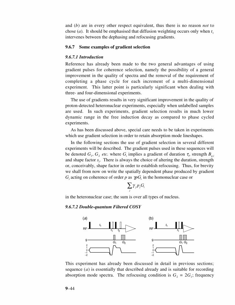
9–44

and (b) are in every other respect equivalent, thus there is no reason not tochose (a). It should be emphasised that diffusion weighting occurs only when t1

intervenes between the dephasing and refocusing gradients.

9.6.7 Some examples of gradient selection

9.6.7.1 Introduction

Reference has already been made to the two general advantages of usinggradient pulses for coherence selection, namely the possibility of a generalimprovement in the quality of spectra and the removal of the requirement ofcompleting a phase cycle for each increment of a multi-dimensionalexperiment. This latter point is particularly significant when dealing withthree- and four-dimensional experiments.

The use of gradients results in very significant improvement in the quality ofproton-detected heteronuclear experiments, especially when unlabelled samplesare used. In such experiments, gradient selection results in much lowerdynamic range in the free induction decay as compared to phase cycledexperiments.

As has been discussed above, special care needs to be taken in experimentswhich use gradient selection in order to retain absorption mode lineshapes.

In the following sections the use of gradient selection in several differentexperiments will be described. The gradient pulses used in these sequences willbe denoted G1, G2 etc. where Gi implies a gradient of duration τi, strength Bg,i

and shape factor si. There is always the choice of altering the duration, strengthor, conceivably, shape factor in order to establish refocusing. Thus, for brevitywe shall from now on write the spatially dependent phase produced by gradientGi acting on coherence of order p as γpGi in the homonuclear case or

γ j j ij

p G∑in the heteronuclear case; the sum is over all types of nucleus.

9.6.7.2 Double-quantum Filtered COSY

g

RF

(a) (b)

t1

G1 G2

1τ 2τ

210

–1–2

g

RFt1

G1 G2

1τ

210

–1–2

This experiment has already been discussed in detail in previous sections;sequence (a) is essentially that described already and is suitable for recordingabsorption mode spectra. The refocusing condition is G2 = 2G1; frequency

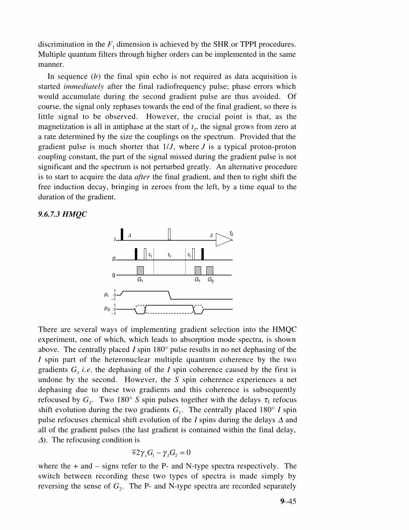
9–45

discrimination in the F1 dimension is achieved by the SHR or TPPI procedures.Multiple quantum filters through higher orders can be implemented in the samemanner.

In sequence (b) the final spin echo is not required as data acquisition isstarted immediately after the final radiofrequency pulse; phase errors whichwould accumulate during the second gradient pulse are thus avoided. Ofcourse, the signal only rephases towards the end of the final gradient, so there islittle signal to be observed. However, the crucial point is that, as themagnetization is all in antiphase at the start of t2, the signal grows from zero ata rate determined by the size the couplings on the spectrum. Provided that thegradient pulse is much shorter that 1/J, where J is a typical proton-protoncoupling constant, the part of the signal missed during the gradient pulse is notsignificant and the spectrum is not perturbed greatly. An alternative procedureis to start to acquire the data after the final gradient, and then to right shift thefree induction decay, bringing in zeroes from the left, by a time equal to theduration of the gradient.

9.6.7.3 HMQC

t2

10

–1

t1

10

–1

∆ ∆I

S

pI

pS

gG1G1 G2

1τ1τ

There are several ways of implementing gradient selection into the HMQCexperiment, one of which, which leads to absorption mode spectra, is shownabove. The centrally placed I spin 180° pulse results in no net dephasing of theI spin part of the heteronuclear multiple quantum coherence by the twogradients G1 i.e. the dephasing of the I spin coherence caused by the first isundone by the second. However, the S spin coherence experiences a netdephasing due to these two gradients and this coherence is subsequentlyrefocused by G2. Two 180° S spin pulses together with the delays τ1 refocusshift evolution during the two gradients G1. The centrally placed 180° I spinpulse refocuses chemical shift evolution of the I spins during the delays ∆ andall of the gradient pulses (the last gradient is contained within the final delay,∆). The refocusing condition is

m2 01 2γ γs IG G− =

where the + and – signs refer to the P- and N-type spectra respectively. Theswitch between recording these two types of spectra is made simply byreversing the sense of G2. The P- and N-type spectra are recorded separately

9–46

and then combined in the manner described in section 9.4.4.2 to give afrequency discriminated absorption mode spectrum.

In the case that I and S are proton and carbon-13 respectively, the gradientsG1 and G 2 are in the ratio 2:±1. Proton magnetization not involved inheteronuclear multiple quantum coherence, i.e. magnetization from protons notcoupled to carbon-13, is refocused after the second gradient G1 but is thendephased by the final gradient G2. Provided that the gradient is strong enoughthese unwanted signals, and the t1-noise associated with them, will besuppressed.

9.6.7.4 HSQC

t2

10

–1

t1

10

–1

Ia

b

y

S

pI

pS

gG

∆2

∆2

∆2

∆2

The sequence above shows the simplest way of implementing gradients into theHSQC experiment. An analysis using product operators shows that at point athe required signal is present as the operator 2IzSz whereas the undesired signal(from I spins not coupled to S spins) is present as Iy. Thus, a field gradientapplied at point a will dephase the unwanted magnetization and leave thewanted term unaffected. This is an example of using gradients not forselection, but for suppression of unwanted magnetization (see section 9.6.3.2).

The main practical difficulty with this approach is that the unwantedmagnetization is only along y at point a provided all of the pulses are perfect; ifthe pulses are imperfect there will be some z-magnetization present which willnot be eliminated by the gradient. In the case of observing proton-13C orproton-15N HSQC spectra from natural abundance samples, the magnetizationfrom uncoupled protons is very much larger than the wanted magnetization, soeven very small imperfections in the pulses can give rise to unacceptably largeresidual signals. However, for globally labelled samples the degree ofsuppression is often sufficient and such an approach is used successfully inmany three- and four-dimensional experiments applied to globally 13C and 15Nlabelled proteins.

The key to obtaining the best suppression of the uncoupled magnetization isto apply a gradient when transverse magnetization is present on the S spin. Anexample of the HSQC experiment utilising such a principle is shown below

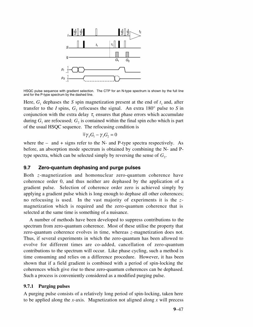
9–47

t2

10

–1

t1

10

–1

I

S

pI

pS

gG1 G2

1τ

∆2

∆2

∆2

∆2

HSQC pulse sequence with gradient selection. The CTP for an N-type spectrum is shown by the full lineand for the P-type spectrum by the dashed line.

Here, G1 dephases the S spin magnetization present at the end of t1 and, aftertransfer to the I spins, G2 refocuses the signal. An extra 180° pulse to S inconjunction with the extra delay τ1 ensures that phase errors which accumulateduring G1 are refocused; G2 is contained within the final spin echo which is partof the usual HSQC sequence. The refocusing condition is

mγ γS IG G1 2 0− =

where the – and + signs refer to the N- and P-type spectra respectively. Asbefore, an absorption mode spectrum is obtained by combining the N- and P-type spectra, which can be selected simply by reversing the sense of G2.

9.7 Zero-quantum dephasing and purge pulses

Both z-magnetization and homonuclear zero-quantum coherence havecoherence order 0, and thus neither are dephased by the application of agradient pulse. Selection of coherence order zero is achieved simply byapplying a gradient pulse which is long enough to dephase all other coherences;no refocusing is used. In the vast majority of experiments it is the z-magnetization which is required and the zero-quantum coherence that isselected at the same time is something of a nuisance.

A number of methods have been developed to suppress contributions to thespectrum from zero-quantum coherence. Most of these utilise the property thatzero-quantum coherence evolves in time, whereas z-magnetization does not.Thus, if several experiments in which the zero-quantum has been allowed toevolve for different times are co-added, cancellation of zero-quantumcontributions to the spectrum will occur. Like phase cycling, such a method istime consuming and relies on a difference procedure. However, it has beenshown that if a field gradient is combined with a period of spin-locking thecoherences which give rise to these zero-quantum coherences can be dephased.Such a process is conveniently considered as a modified purging pulse.

9.7.1 Purging pulses

A purging pulse consists of a relatively long period of spin-locking, taken hereto be applied along the x-axis. Magnetization not aligned along x will precess

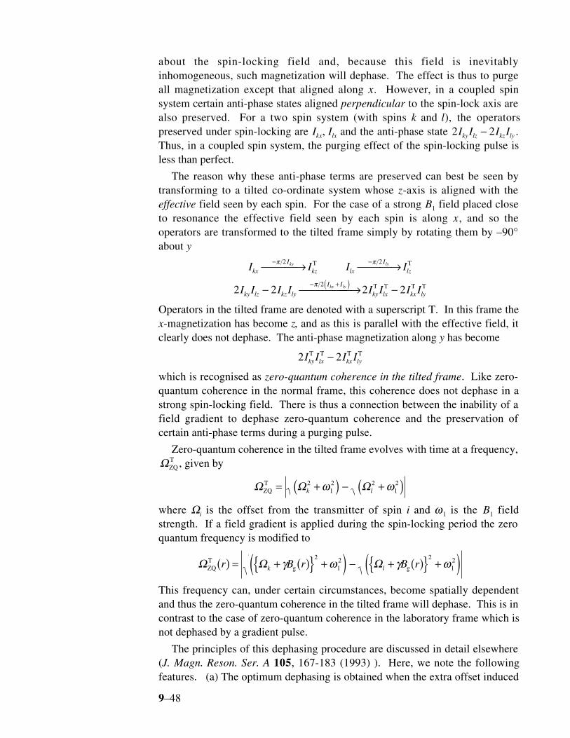
9–48

about the spin-locking field and, because this field is inevitablyinhomogeneous, such magnetization will dephase. The effect is thus to purgeall magnetization except that aligned along x. However, in a coupled spinsystem certain anti-phase states aligned perpendicular to the spin-lock axis arealso preserved. For a two spin system (with spins k and l), the operatorspreserved under spin-locking are Ikx, Ilx and the anti-phase state 2 2I I I Iky lz kz ly− .Thus, in a coupled spin system, the purging effect of the spin-locking pulse isless than perfect.

The reason why these anti-phase terms are preserved can best be seen bytransforming to a tilted co-ordinate system whose z-axis is aligned with theeffective field seen by each spin. For the case of a strong B1 field placed closeto resonance the effective field seen by each spin is along x, and so theoperators are transformed to the tilted frame simply by rotating them by –90°about y

I I I I

I I I I I I I I

kx

I

kz lx

I

lz

ky lz kz ly

I I

ky lx kx ly

ky ly

ky ly

− −

− +( ) → →

− → −

π π

π

2 2

22 2 2 2

T T

T T T T

Operators in the tilted frame are denoted with a superscript T. In this frame thex-magnetization has become z, and as this is parallel with the effective field, itclearly does not dephase. The anti-phase magnetization along y has become

2 2I I I Iky lx kx lyT T T T−

which is recognised as zero-quantum coherence in the tilted frame. Like zero-quantum coherence in the normal frame, this coherence does not dephase in astrong spin-locking field. There is thus a connection between the inability of afield gradient to dephase zero-quantum coherence and the preservation ofcertain anti-phase terms during a purging pulse.

Zero-quantum coherence in the tilted frame evolves with time at a frequency,ΩZQ

T , given by

Ω Ω ΩZQT = +( ) − +( )k l

212 2

12ω ω

where Ωi is the offset from the transmitter of spin i and ω1 is the B1 fieldstrength. If a field gradient is applied during the spin-locking period the zeroquantum frequency is modified to

Ω Ω ΩZQT

g gr B r B rk l( ) = + ( ) +( ) − + ( ) +( )γ ω γ ω2

12 2

12

This frequency can, under certain circumstances, become spatially dependentand thus the zero-quantum coherence in the tilted frame will dephase. This is incontrast to the case of zero-quantum coherence in the laboratory frame which isnot dephased by a gradient pulse.

The principles of this dephasing procedure are discussed in detail elsewhere(J. Magn. Reson. Ser. A 105, 167-183 (1993) ). Here, we note the followingfeatures. (a) The optimum dephasing is obtained when the extra offset induced

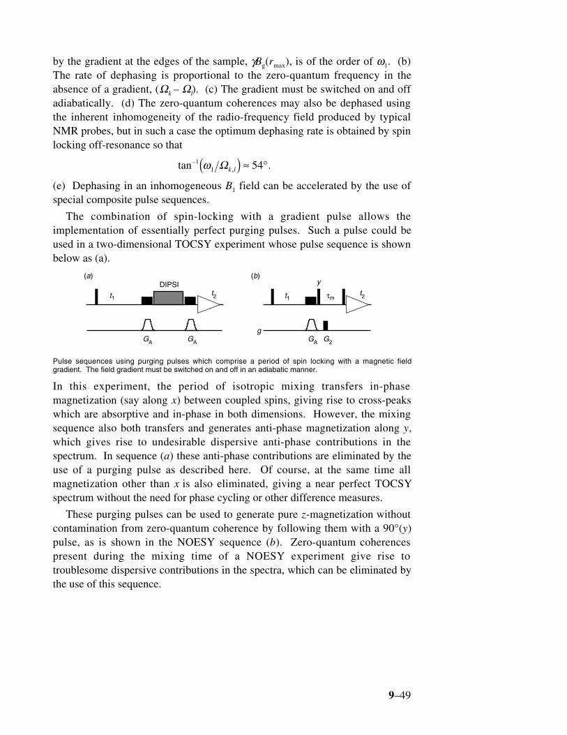
9–49

by the gradient at the edges of the sample, γBg(rmax), is of the order of ω1. (b)The rate of dephasing is proportional to the zero-quantum frequency in theabsence of a gradient, (Ωk – Ωl). (c) The gradient must be switched on and offadiabatically. (d) The zero-quantum coherences may also be dephased usingthe inherent inhomogeneity of the radio-frequency field produced by typicalNMR probes, but in such a case the optimum dephasing rate is obtained by spinlocking off-resonance so that

tan–,

11 54ω Ωk l( ) ≈ °.

(e) Dephasing in an inhomogeneous B1 field can be accelerated by the use ofspecial composite pulse sequences.

The combination of spin-locking with a gradient pulse allows theimplementation of essentially perfect purging pulses. Such a pulse could beused in a two-dimensional TOCSY experiment whose pulse sequence is shownbelow as (a).

t1 τm

gGAGA GA G2

y

t2t1t2

DIPSI(a) (b)

Pulse sequences using purging pulses which comprise a period of spin locking with a magnetic fieldgradient. The field gradient must be switched on and off in an adiabatic manner.

In this experiment, the period of isotropic mixing transfers in-phasemagnetization (say along x) between coupled spins, giving rise to cross-peakswhich are absorptive and in-phase in both dimensions. However, the mixingsequence also both transfers and generates anti-phase magnetization along y,which gives rise to undesirable dispersive anti-phase contributions in thespectrum. In sequence (a) these anti-phase contributions are eliminated by theuse of a purging pulse as described here. Of course, at the same time allmagnetization other than x is also eliminated, giving a near perfect TOCSYspectrum without the need for phase cycling or other difference measures.

These purging pulses can be used to generate pure z-magnetization withoutcontamination from zero-quantum coherence by following them with a 90°(y)pulse, as is shown in the NOESY sequence (b). Zero-quantum coherencespresent during the mixing time of a NOESY experiment give rise totroublesome dispersive contributions in the spectra, which can be eliminated bythe use of this sequence.