Coherence in neutrino oscillations

Joonas Ilmavirta

Kandidaatin tutkielmaJyväskylän yliopisto, Fysiikan laitos

4.2.2011Ohjaaja: Jukka Maalampi

Abstract

The theory of neutrino oscillations has turned out to be the most rea-

sonable explanation to the observed violations in lepton number con-

servation of solar and atmospheric neutrino �uxes. A derivation of

the most important results of this theory is �rst given using a plane

wave treatment and subsequently using a three-dimensional shape-

independent wave packet approach. Both methods give the same os-

cillation patterns, but only the latter one serves as a decent starting

point for analyzing coherence in neutrino oscillations.

A numerical analysis of the oscillation patterns on various distance

scales is also given to graphically illustrate the phenomenon of neutrino

oscillation and loss of coherence in it.

Several coherence conditions related to wave packet separation and

the uncertainties of energy and momentum in the mass states pro-

duced in a weak charged current reaction are derived. In addition, a

new limit is obtained for neutrino �ux, beyond which the oscillation

pattern may be washed out due to the overlap of the wave packets de-

scribing neutrinos originating from di�erent reactions. Whether or not

any phenomena will take place in the case of very high �ux remains

uncertain, because the �ux limit is beyond the scope of any modern

neutrino experiment.

Tiivistelmä

Neutriino-oskillaatiot tarjoavat luontevimman selityksen havaituille lep-

tonilukujen säilymislain rikkoutumiselle, joka on havaittu auringosta

ja ilmakehästä tulevissa neutriinoissa. Neutriino-oskillaatioiden teo-

rian tärkeimmät tulokset johdetaan ensin tasoaaltoapproksimaatiossa

ja sen jälkeen käyttäen kolmiulotteisia mielivaltaisen muotoisia aalto-

paketteja. Oskillaatiota ja siihen liittyvää koherenssin häviämistä ha-

vainnollistetaan numeerisilla laskuilla tuotetuin kuvaajin.

Oskillaatioille johdetaan erilaisia koherenssiehtoja liittyen aaltopa-

kettien erkanemiseen sekä energian ja liikemäärän epätarkkuuteen. Li-

säksi löydetään uusi raja neutriinovuolle, jonka yläpuolella oskillaatiot

saattavat kadota. Se, tapahtuuko näin suurilla voilla kiinnostavia il-

miöitä, jää epävarmaksi, sillä nykyisillä koejärjestelyillä asiaa ei ole

mahdollista tutkia.

Summarium

Violatio observata conservationis numerorum leptorum in neutrinis de

Sole et atmosphaera devolantibus simplicissime explicari potest oscil-

latione neutrinorum. Eventus principales theoriae oscillationum neu-

trinorum deducuntur primum undulis planis, deinde fascibus undu-

latoriis tridimensionalibus cuiuslibet formae. Oscillatio amissioque

cohaerentiae in ea graphice illustrantur.

Variae necessitates cohaerentiae ad dissociationem fascium undu-

latoriorum et incertitatem energiae et motus pertinentes deducuntur,

necnon novus �nis �umini neutrinonum, super quem oscillationes abo-

lescere possunt. An vero abolescant necne, incertum relinquitur, quia

tale �umen longe extra facultates hodiernas mensurandi manet.

3

Contents

1 Introduction 5

2 Plane wave approximation 6

2.1 The standard formula for neutrino oscillations . . . . . . . . . 62.2 Massive neutrinos of equal energy . . . . . . . . . . . . . . . . 72.3 Massive neutrinos of equal momentum . . . . . . . . . . . . . 82.4 An overview to the physics behind the assumptions . . . . . . 8

3 Wave packets 9

3.1 The need for the wave packet treatment . . . . . . . . . . . . 93.2 Wave packet spreading . . . . . . . . . . . . . . . . . . . . . . 103.3 Neutrino oscillations in wave packet treatment . . . . . . . . . 11

3.3.1 Produced and detected states . . . . . . . . . . . . . . 113.3.2 From transition amplitude to probability . . . . . . . . 123.3.3 Calculating the interference integral . . . . . . . . . . 143.3.4 Normalization . . . . . . . . . . . . . . . . . . . . . . . 16

3.4 Gaussian wave packets . . . . . . . . . . . . . . . . . . . . . . 17

4 Coherence 17

4.1 General remarks . . . . . . . . . . . . . . . . . . . . . . . . . 174.2 Coherence in plane wave approximation . . . . . . . . . . . . 184.3 Coherence in wave packet treatment . . . . . . . . . . . . . . 194.4 Restoration of coherence at detection . . . . . . . . . . . . . . 204.5 Wave packet spreading . . . . . . . . . . . . . . . . . . . . . . 214.6 The case of high �ux . . . . . . . . . . . . . . . . . . . . . . . 214.7 Summary . . . . . . . . . . . . . . . . . . . . . . . . . . . . . 22

5 Numerical analysis 23

5.1 Preliminary assumptions and mixing parameters . . . . . . . 235.2 Neutrino oscillations on di�erent scales . . . . . . . . . . . . . 25

6 Coherence in future experiments 28

4

1 Introduction

Despite the great success of the Standard Model (SM), not all of its predic-tions are in accordance with phenomena observed in Nature. It has turned,contrary to the predictions of SM, out that neutrinos do have mass andthat none of the three lepton numbers is conserved � in the case of sterileneutrinos even the sum of these three lepton numbers is not conserved. In-deed, neutrino oscillations were the �rst evidence that something must belacking from the SM [1]. New theoretical ideas are needed to explain thesephenomena.

Observations of atmospheric and solar neutrinos indicate violations inlepton number conservation. In the former case, the observed �ux of muonneutrinos νµ on the ground is substantially smaller than what is estimatedto be produced in interactions of cosmic rays in the atmosphere. In thelatter case a fraction of the electron neutrinos created in the Sun seems todisappear on its way to Earth (for experimental results, see eg. [2]), whichwas known as the solar neutrino problem (for a more thorough discussionof neutrino astronomy, see [3]). In both phenomena some of the producedneutrinos transform into neutrinos of other �avors as they propagate throughspace, and they are thus merely two incarnations of the same phenomenon,neutrino oscillation.

The most natural explanation to this and other observed phenomenaunpredicted by the sole SM arises from the concept of mixed and massiveneutrinos [4]. According to this explanation, the weak interaction eigenstates|νe〉, |νµ〉, and |ντ 〉 (i.e. the �avor states) have no well-de�ned mass, but theirsuperpositions do. The �avor states |να〉 (α = e, µ, τ) are expressed in termsof the mass states |νi〉 as [5]

|να〉 =N∑i=1

U∗αi |νi〉 , (1)

where U is the neutrino mixing matrix or the Pontecorvo�Maki�Nakagawa�Sakata matrix [6]. The matrix U is unitary and can be chosen real andorthogonal if there is no CP-violation in neutrino mixing [7, 8]. For de�-niteness, the mixing matrix U is taken to be a unitary but not necessarilyreal 3×3-matrix. Both the �avor and mass neutrino states are orthonormal,〈να|νβ〉 = δαβ and 〈νi|νj〉 = δij .

A �avor antineutrino state |νl〉 can be expressed in terms of antineutrinomass states as [9]

|να〉 =

N∑i=1

Uαi |νi〉 , (2)

where the only change to Eq. (1) is the absence complex conjugation in themixing matrix elements. If the mixing matrix is taken to be real, the mixing

5

schemes for neutrinos and antineutrinos are exactly the same. The timeevolution of an antiparticle state is similar to that of a particle state1, sothe oscillation pattern will be the same. Therefore only neutrinos will beconsidered in the following.

An analogue of neutrino mixing is found in classical mechanics: the massstates can be identi�ed with normal coordinates in a system of coupled os-cillators, whereas �avor states describe individual oscillators. The obtainedoscillation phenomenon bears a striking resemblance to that of neutrino os-cillations, although quantum mechanics or quantum �eld theory is needed todescribe neutrinos. A nice discussion of classical coupled oscillators is givenin [10].

The �avor space � which is the state space in the crudest approximation� is usually taken to be three-dimensional. If N > 3, there are sterile neu-trinos, ��avors� that do not enter the SM electroweak interaction Lagrangianand therefore do not interact [6]. On the basis of experimental data it is notyet possible to conclude whether sterile neutrinos exist or not [11].

The origin and exact values of the neutrino masses is a vast area oftheoretical [12] and experimental [11] research, which will not be dwelledinto in any more detail than required for the other considerations.

It is not even known whether neutrinos are Dirac or Majorana particles.In the latter case neutrinos are their own antiparticles and in the former casenot [12]. Other standard model fermions are known to be Dirac particles,but it is believed that neutrinos make an exception.

2 Plane wave approximation

2.1 The standard formula for neutrino oscillations

The simplest insight to neutrino oscillations is provided by the study ofthe time evolution of �avor plane waves. In fact, even the formalism ofplane waves simpli�es to a three-state system of the �avor neutrinos, andthe spatial dependence of the phenomenon is later introduced by an ad hoc

procedure.

As the �avor neutrino states have no well-de�ned mass, they have nowell-de�ned energy and therefore their time dependence is more complexthan that of a simple phase factor. The mass states do, however, have themost simple time evolution.

Consider a neutrino state |ν(t)〉 and assume that it is created at t = 0 asa pure �avor state of �avor α, i.e. |ν(0)〉 = |να〉. As stated in Eq. (1), this

1For a particle state |φ(t)〉 = e−iEt |φ〉 and for an antiparticle |φ(t)〉 = e+iEt |φ〉. Com-plex conjugating all phases in the calculations will lead to the same absolute values ofinner products.

6

state is the superposition of massive neutrinos,

|ν(0)〉 =3∑i=1

U∗αi |νi〉 . (3)

Given that the mass state | νi〉 has the energy Ei, the time evolution of thestate is simply given by

|ν(t)〉 =∑i

U∗αie−iEit |νi〉 . (4)

The bra vector corresponding to the neutrino of �avor β is found by conju-gating (1):

〈νβ| =∑j

Uβj 〈νj | . (5)

Thus the probability of �nding a neutrino in the �avor β at a time t is givenby

P (να → νβ; t) = |〈νβ|ν(t)〉|2 =∑i,j

U∗αiUβjUαjU∗βje−i(Eit−Ejt). (6)

2.2 Massive neutrinos of equal energy

A crucial but dubious step in the calculation of the probability is to intro-duce relations between the properties of di�erent neutrinos mass states andbetween time and space. This transforms the �avor detection probabilityfunction in Eq. (6) into a function of distance and a kinematical variabledescribing the produced neutrino.

A common way to do this is to assume that all the neutrino mass stateshave the same energy. Arguments supporting this idea are presented, forexample, in [13, 14, 15], although some consider it unphysical [5]. Thesearguments will be discussed more thoroughly in section 2.4.

Elementary relativistic kinematics shows that a particle of mass m andenergy E travels at the speed

v =

√1− m2

E2. (7)

If L is the distance traveled by the neutrino between production and detec-tion points and every massive neutrino has the energy E, then

Eti − Etj =EL

(1− m2

i

E2

)−1/2

− EL

(1−

m2j

E2

)−1/2

≈EL(

1 +m2i

2E2

)− EL

(1 +

m2j

2E2

)

=L(m2

i −m2j )

2E, (8)

7

which is accurate to the �rst order in squared neutrino masses. Denoting∆m2

ij = m2i −m2

j , Eq. (6) leads to the standard formula for neutrino oscil-lations:

P (να → νβ;L) =∑i,j

U∗αiUβiUαjU∗βje−i

L∆m2ij

2E . (9)

2.3 Massive neutrinos of equal momentum

Some authors consider the equal energy assumption unphysical [5] and in-stead assume that the di�erent mass states have the same momentum in-stead. Some [7] use the assumption for other than physical reasons such assimplicity. These di�erent assumptions of equal energy or momentum havelittle or no di�erence in either the di�culty of the calculations or the result.

Let every mass state |νi〉 in Eq. (4) have the same momentum p. Theenergies of the states are then

Ei =√p2 +m2

i ≈ p+m2i

2p(10)

and so

Eit− Ejt ≈t∆m2

ij

2p. (11)

If one further assumes that L ≈ t, i.e. v ≈ 1, one arrives to the formula

P (να → νβ;L) =∑i,j

U∗αiUβiUαjU∗βje−i

L∆m2ij

2p , (12)

which only di�ers from Eq. (9) in that E has been replaced by p. Bearingin mind that E ≈ p for ultrarelativistic neutrinos, these two results are thesame in the approximation used. Since L∆m2

ij/2p is already �rst order insquared neutrino masses, the corrections from changing p to E are negligible.

Some authors think that these two approaches give exactly the sameresult and represent essentially the same physics, although it may be better todistinguish these two approaches [16]. This comparison is, however, beyondthe scope of the present analysis.

2.4 An overview to the physics behind the assumptions

Plane waves are not localized, and in fact even non-propagating [17], but onedoes wish to calculate distance-dependent probabilities in order to be ableto make predictions for neutrino oscillation experiments.

In the above derivation of the oscillation probability formula it was nec-essary to assume that the mass states have either equal energy or equalmomentum. It sounds plausible that they are both almost equal. As the

8

wave packet treatment will show, this is su�cient to obtain the standardformula of Eq. (9).

Even if massive neutrinos have equal energy or equal momentum in someframe of reference, they will not in general do so after a Lorentz boost [9].Therefore assumptions of equal momentum or equal energy are valid onlyin the framework of a speci�c frame. De�ning such a frame is a dubiousad hoc procedure. In the wave packet treatment no such assumption isneeded to arrive at the probability formula (9). In a generic case of three�avor neutrinos there will be no frame where the massive neutrinos haveequal energy [17]. Frame independence allows for much more �exibility inapplying the theory to any practical situation.

Coherence can only be given a rigorous treatment using wave packets,and this will be done in section 4. A simpli�ed coherence condition will bederived in terms of the plane wave approximation, but such a model cannotproperly describe the coherence of massive neutrinos at a given time andpoint.

A general assumption made in most neutrino oscillation investigations isthat neutrinos are ultrarelativistic. Not all neutrinos need be, but since onlyneutrinos of about 100 keV or more energy can be observed [5] and neutrinomasses are at most around 2 eV [11], this approximation is very good for allobservable neutrinos of the stardard type.

3 Wave packets

3.1 The need for the wave packet treatment

As discussed in Section 2.4, the plane wave approximation requires numerousphysically questionable assumptions. Usually neutrinos have neither equalenergy nor equal momentum [9], and with wave packets no such assumptionis needed. Also, no trajectory condition such as L ≈ t needs to be imposedby hand, because such a trajectory equation can be derived from the timeevolution of the wave packets.

There are two highly unphysical consequences of approximating neutrinosby plane waves. First, in this approach the neutrino has a well-de�nedmomentum and thus completely loses its locality. Second, the source of aplane wave has to vibrate in the same manner for in in�nite period of time[18]. It is easy to understand that the production process of a neutrino isspatially localized and spans only over a �nite period of time.

9

3.2 Wave packet spreading

Wave packet spreading can be analyzed [16] by considering a wave functionin the momentum representation having a Gaussian wave packet form

f(p) =1√√πσp

exp

((p− p0)2

2σ2p

), (13)

where p0 is the mean momentum and σp is the momentum uncertainty. Fromthis the corresponding wave function in coordinate representation is obtainedby Fourier transform:

ψ(x, t) =1√2π

∫dpf(p)ei(px−Et). (14)

Assuming that the particle in question has a mass m, the energy of theparticle is E = E(p) =

√p2 +m2. Denoting E0 = E(p0), this expression is

expanded around the peak of f(p) as

E(p) ≈ E0 +dE

dp

∣∣∣∣p=p0

(p− p0) +d2E

dp2

∣∣∣∣p=p0

(p− p0)2

2. (15)

Expanding only to the �rst order gives wave packets of constant shape, whilethe second order term allows one to analyze the spreading [16]. Carryingout the di�erentiations and introducing v = p0/E0 (the group velocity of theparticle as discussed in Section 3.3.1), the energy becomes

E(p) ≈ E0 + v(p− p0) +1− v2

E0

(p− p0)2

2. (16)

Collecting Eqs. (13), (14), and (16) and carrying out the integration yields

ψ(x, t) ≈ 14√π

√p0σp

p0 + iσ2ptv(1− v2)

× exp

(2ip0tv + σ2

pt2(3v2 − 2)− (2ip0 + 2σ2

ptv3)x+ σ2

px2

2p−10 (p0 + iσ2tv(1− v2))

). (17)

The squared modulus of the wave function ψ(x, t) gives the transition prob-ability density ρ,

ρ(x, t) =1√π

p0σp√p2

0 + σ4pt

2v2(1− v2)2

× exp

(− (x− tv)2

σ−2p (1 + σ4

pt2v2 (1− v2)2 /p2

0)

). (18)

10

This implies that the length of the wave packet σx behaves as

σx(t) = σx0

√1 +

σ4pt

2v2 (1− v2)2

p20

. (19)

The application of this result to neutrino oscillations will be discussed inSection 4.5.

3.3 Neutrino oscillations in wave packet treatment2

3.3.1 Produced and detected states

Neutrino oscillations are now considered in wave packet formalism as opposedto the plane waves used in Section 2. As in the plane wave approach, a �avorneutrino state of �avor α is created at the origin of a frame of reference whent = 0. The corresponding state is decomposed to massive neutrino states,which are described by wave packets ψSi (~x, t) (superscript S refers to thesource):

|ν(~x, t)〉 =∑i

U∗αiψSi (~x, t) |νi〉 , (20)

where the wave packets are described by momentum distribution functionsfSi (~p) as

ψSi (~x, t) =

∫d3~p

(2π)3/2fSi (~p− ~pSi )ei(~p · ~x−Ei(p)t), (21)

where ~pSi is the mean momentum and Ei(p) =√p2 +m2

i .

In the above the function fSi (~p) is strongly peaked at the origin; takingfSi (~p) = δ(3)(~p) would lead to plane waves with de�nite momenta. It is alsoassumed that the peak of fSi (~p− ~pSi ) is not near the origin, that is σSpi � pSi .This can be justi�ed by the ultrarelativistic nature of detectable neutrinos.

Since the above integral is assumed to be strongly suppressed outside~p ≈ ~pSi , one may expand the energy as

Ei(p) = Ei(pSi ) +

∂Ei(p)

∂~p

∣∣∣∣~pSi

· (~p− ~pSi ). (22)

Di�erentiating Ei(p) gives

∂Ei(p)

∂~p

∣∣∣∣~pSi

=~pSi

Ei(pSi ). (23)

This derivative is the group velocity ~vgi of the wave packet.

2This discussion mostly follows that of [17].

11

Working to the �rst order squared neutrino masses, one may write ~p · ~x−Ei(p)t = ~pSi · ~x + (~p − ~pSi ) · ~x − (Ei(p

Si ) + ~vgi · (~p − ~pSi ))t, and thus the wave

packet (21) can be rewritten as

ψSi (~x, t) = ei(~pSi · ~x−Ei(p

Si ))gSi (~x− ~vgit), (24)

where

gSi (~x) =

∫d3~p

(2π)3/2fSi (~p)ei~p · ~x. (25)

In this approximation the shape of the wave packet is preserved [17]. Thisis evident from the fact that the shape factor of the wave packet dependson time and place only through the combination ~x − ~vgit � this form alsoexplains why ~vgi is the group velocity.

A detecting particle is placed at ~x = ~L. In most cases of interest, thedetected neutrino state |νβ〉 is essentially time-independent [17]. Thus, wehave in analogue to to the state |ν(~x, t)〉 discussed above (D refers to thedetecting particle),∣∣∣νβ(~x− ~L)

⟩=∑i

U∗βiψDi (~x− ~L) |νi〉 (26)

ψDi (~x− ~L) =

∫d3~p

(2π)3/2fDi (~p− ~pDi )ei~p · (~x−~L). (27)

It is assumed that the momentum distribution functions fDi are stronglypeaked around the origin. As above, the wave packet can be approximatedas

ψDi (~x− ~L) = ei~pDi · (~x−~L)gDi (~x− ~L), (28)

where

gDi (~x) =

∫d3~p

(2π)3/2fDi (~p)ei~p · ~x. (29)

3.3.2 From transition amplitude to probability

By projecting the produced, time-evolved neutrino state (20) to the detectedstate (26), one arrives at the transition amplitude

Aα→β(~L, t) =

∫d3~x

⟨νβ(~x− ~L)

∣∣∣ν(~x, t)⟩. (30)

In order to evaluate this amplitude, one has to evaluate integrals of the form∫d3~xψD∗i (~x− ~L)ψSi (~x, t). (31)

Using the expressions (24) and (28) and noting that

(~pSi · ~x−Ei(pSi )t)−~pDi · (~x− ~L) = ~pSi · ~L−Ei(pSi )t+(~pSi −~pDi ) · (~x− ~L), (32)

12

one may write

ψD∗i (~x− ~L)ψSi (~x, t) = gD∗i (~x− ~L)gSi (~x−~vgit)ei(~pSi · ~L−Ei(p

Si )t)ei(~p

Si −~pDi ) · (~x−~L).

(33)The orthogonality of massive neutrino states gives then for the transitionamplitude Aα→β the form

Aα→β(~L, t) =∑i

U∗αiUβiei(~pSi · ~L−Ei(p

Si )t)Gi(~L− ~vgit) (34)

where

Gi(~L) =

∫d3~xgD∗i (~x)gSi (~x+ ~L)ei(~p

Si −~pDi ) · ~x. (35)

The exact moment of production or detection is usually not measured inneutrino experiments, so the probability of detecting the �avor β at thedetector is given by the time integral

P (να → νβ; ~L) =

∫ ∞−∞

dt∣∣∣Aα→β(~L, t)

∣∣∣2 . (36)

Denoting Ei = Ei(pSi ) and de�ning

Iij(~L) =

∫ ∞−∞

dtG∗j (~L− ~vgjt)Gi(~L− ~vgit)e−i∆φij(~L,t) (37)

with

∆φij = (Ei − Ej)t− (~pSi − ~pSj ) · ~L, (38)

the probability becomes

P (να → νβ; ~L) =∑i,j

U∗αiUβiUαjU∗βjIij(

~L). (39)

The similarity of this formula to the standard formula for neutrino oscilla-tions given in Eq. (9) is immediately noted and it will be further strength-ened by the forms of Iij(~L) obtained in Sections 3.3.3 and 3.4, which givethe phase factor of the standard formula. The main phenomenon in neutrinooscillations is due to the phase factor ∆φij , and it should be noted that itsform in Eq. (38) is Lorentz invariant, removing the issue of Lorentz boostsinvalidating the calculations.

The integral Iij(~L) describes how much the wave packets of ith andjth massive neutrinos overlap, and is thus called an interference integral.For a discussion of why the interference integral Iij(~L) and therefore theprobability is Lorentz-invariant, see [17].

13

3.3.3 Calculating the interference integral

To get the probability (39) in a simpler form, the di�erence of momentabetween produced and detected massive neutrino states is denoted by ~δi =~pSi − ~pDi . With this and ∫

d3~xe−i~y · ~x = (2π)3δ(3)(~y) (40)

for the Dirac's delta function one may write

Gi(~L) =

∫d3~xgD∗i (~x)gSi (~x+ ~L)ei(~p

Si −~pDi ) · ~x

=

∫d3~x

∫d3~p

(2π)3/2

∫d3~q

(2π)3/2fD∗i (~p)fSi (~q)

× e−i~p · ~xei~q · (~x+~L)ei~δi · ~x

=

∫d3~p

∫d3~qδ(3)(~p− ~δi − ~q)fD∗i (~p)fSi (~q)ei~q · ~L

=

∫d3~qfD∗i (~q + ~δi)f

Si (~q)ei~q · ~L, (41)

where Eqs. (25), (29) and (35) have been used. This with the one-dimensionalform of Eq. (40) leads to

Iij(~L) =

∫ ∞−∞

dt

∫d3~pfDj (~p+ ~δj)f

S∗j (~p)e−i~p · (~L−~vgjt)

×∫

d3~qfD∗i (~q + ~δi)fSi (~q)ei~q · (~L−~vgit)e−i((Ei−Ej)t−(~pSi −~pSj ) · ~L)

= 2π

∫d3~p

∫d3~qfDj (~p+ ~δj)f

S∗j (~p)fD∗i (~q + ~δi)f

Si (~q)

× δ(~q ·~vgi − ~p ·~vgj + ∆Eij)ei(~q−~p+∆~pSij) · ~L. (42)

To continue further, a choice of coordinates is made such that ~vgj = zvgj ,where z is the unit vector in z-direction. The vector ~p is expressed as ~p =~p‖z + ~p⊥z and others similarly. The following property is easily derived:

∫d3~xf(~x)δ(~x · zz − a) =

1

z

∫d2~x⊥zf(~x0 + ~x⊥z), (43)

where ~x0 is any vector such that ~x0 · zz = a and f is a su�ciently smoothfunction. In the ~p-integration of Eq. (42) one can choose ~p0 = (~q ·~vgi +∆Eij)z/vgj , which clearly satis�es ~p0 · zvgj = ~q ·~vgi + ∆Eij . Thus the eval-

14

uation of Iij may be continued as

Iij(~L) =2π

vgj

∫d2~p⊥z

∫d2~q⊥z

∫d~q‖zf

Dj

(~p⊥z + (~q ·~vgi + ∆Eij)

z

vgj+ ~δj

)× fS∗j

(~p⊥z + (~q ·~vgi + ∆Eij)

z

vgj

)fD∗i (~q⊥z + ~q‖z + ~δi)

× fSi (~q⊥z + ~q‖z)ei

(~q⊥z+~q‖z−

(~p⊥z+(~q ·~vgi+∆Eij) z

vgj

)+∆~pSij

)· ~L

=2π

vgjei

(∆~pSij−∆Eij

zvgj

)· ~L ∫

d2~p⊥ze−i~p⊥z · ~L

×∫

d2~q⊥zei

(~q⊥z−~q⊥z ·~vgi z

vgj

)· ~L ∫

d~q‖zei

(~q‖z−~q‖z ·~vgi z

vgj

)· ~L

× fDj(~p⊥z + (~q ·~vgi + ∆Eij)

z

vgj+ ~δj

)fD∗i (~q + ~δi)

× fS∗j(~p⊥z + (~q ·~vgi + ∆Eij)

z

vgj

)fSi (~q). (44)

It is assumed that ~vgi ‖ ~vgj , that is ~vgi⊥z = 0, which seems physicallyplausible. Under this assumption the phase factor in front of the integralsabove becomes (∆~pSij−∆Eij z/vgj) · ~L = (∆pSij−∆Eij/vgj)z · ~L. To the �rstorder in squared neutrino masses one may also approximate

∆Eij =E(pSi ,m2i )− E(pSj ,m

2j )

≈ ∂E(p,m2)

∂p

∣∣∣∣pSj ,m

2j

(pSi − pSj ) +∂E(p,m2)

∂m2

∣∣∣∣pSj ,m

2j

(m2i −m2

j )

= vgj∆pSij +

1

2Ej∆m2

ij , (45)

where E(p,m2) =√p2 +m2. Further noting that pSj = vgjEj , one obtains

Iij(~L) =2π

vgje−i

∆m2ij

2p |~L⊥z|∫

d2~p⊥ze−i~p⊥z · ~L

∫d2~q⊥ze

i~q⊥z · ~L

×∫

d~q‖zei

(~q‖z−~q‖z · z vgi

vgjz

)· ~L

× fDj(~p⊥z + (~q‖z · zvgi + ∆Eij)

z

vgj+ ~δj

)fD∗i (~q⊥z + ~q‖z + ~δi)

× fS∗j(~p⊥z + (~q‖z · zvgi + ∆Eij)

z

vgj

)fSi (~q⊥z + ~q‖z), (46)

where p = pSj ≈ 12(pSi + pSj ) (used only to divide ∆m2

ij this approximation

for pSj is valid to the �rst order in squared masses). It is rather convenient to

15

consider propagation in only one spatial dimension, which is a very good ap-proximation when the distance between the production and detection of theneutrino is macroscopic [17]. Taking the one-dimensional version of Eq. (42)and carrying out the p-integration simpli�es the previous equation to

Iij(L) =2π

vgje−i

∆m2ij

2pL∫

dqeiq

(1−

vgivgj

)LfDj

(qvgivgj

+∆Eijvgj

+ δj

)× fD∗i (q + δi)f

S∗j

(qvgivgj

+∆Eijvgj

)fSi (q). (47)

This calculation gives Eq. (39) a form very similar to that of Eq. (9).

The plane wave result of oscillation probabilities is obtained by lettingvgi/vgj → 1 and assuming that the shape factors become the same, i.e.

fS,Di (p) = fS,Dj (p). See [17] for a description of how the latter assumptionsfollows from the former one. Using the normalization (50), the whole ex-pression in Eq. (47) excluding the �rst phase factor tends to unity, leadingto Iij(L) = exp(−i∆m2

ijL/2p). This is indeed the same formula obtained byusing the plane wave approach.

3.3.4 Normalization

Di�erent normalizations have been proposed for the momentum distributionfunctions fSi , for example [16]∫

dpfSi (p) =√

2π, (48)∫dp∣∣fSi (p)

∣∣2 = 1, (49)

and [17] ∫dt∣∣∣Gi(~L− ~vgit)∣∣∣2 = 1. (50)

Imposing such a normalization condition by hand is considered inconsistent.Instead, one should derive them from the temporal response function of thedetector [17] or from a �eld theoretical treatment of the processes of neutrinocreation, propagation and detection [19].

Fortunately, it is not entirely necessary dwell into the subtleties of nor-malization. Discussion of coherence, for example, does not require the cal-culation of any normalization factors. Also, in many applications one maynormalize the probabilities themselves at the very end of the calculationswithout a need for a more explicit treatment. Terms of order O(mν/Eν) canbe neglected in the probabilities (but not the phase and coherence factors),because no detection apparatus has the accuracy to observe such subtle phe-nomena, and a misnormalization of this order is therefore rather insigni�cant.

16

3.4 Gaussian wave packets

It is usually assumed [17] that wave packets have a Gaussian form, e.g. inone dimension [16]

fSi (p) =

√1√πσSpi

e−12

((p−pSi )/σSpi

)/2. (51)

If one de�nes �mean� group velocities as follows

vgij =vgi(σ

Spi)

2 + vgj(σSpj )

2

(σSpi)2 + (σSpj )

2(52a)

v′gij =(vgiσ

Spi)

2 + (vgjσSpj )

2

vgi(σSpi)2 + vgj(σSpj )

2(52b)

and assumes pSi = pDi , the interference integral Iij(L) turns out to be [16]

Iij(L) =

√2ηiηj

vgivgj(η2i + η2

j )

× exp

(−iL

(∆m2

ij

pSi + pSj−

(v−1gi − v

−1gj )(Ei − Ej)(pSi η2

i − pSj η2j )

(pSi + pSj )(η2i + η2

j )

))

× exp

(−

(v−1gi − v

−1gj )2L2

2(η2i + η2

j )

)exp

(−

(Ei − Ej)2η2i η

2j

2(η2i + η2

j )

), (53)

with ηi = (vgiσSpi)−1 in the notation used in Section 3.3.

This result contains essentially the same physics as the more generalresult in Eq. (47), as will be discussed shortly, but this more explicit formallows numerical treatment in Section 5, which cannot be done for genericwave packets.

4 Coherence

4.1 General remarks

In quantum mechanics the coherence of two states is essentially their abil-ity to interfere. Fully coherent states can be described by a superpositionof the states, and interference may take place. If the states are, instead,fully incoherent, there will be no interference. If the states are somehowspatially localized, overlap in the coordinate wave functions is necessary forcoherence if the measurement process is spatially localized. A measurementthat determines which of the states is in question destroys coherence � thishappens in the double-slit experiment if the slit is determined and similarlyin neutrino oscillations if the mass state is determined.

17

For two wave packets of massive neutrinos to be coherent they needto overlap signi�cantly. If the wave packets have slightly di�erent groupvelocities, they will slowly separate. When the wave packets become spatiallytoo separated and thus incoherent, no more oscillations are observed. It musthowever be born in mind that these wave packets describe massive neutrinos,and thus have no well-de�ned �avor. Flavor measurement is therefore notdeterministic even after coherence is lost, nor is it impossible to detect achange in �avor.

4.2 Coherence in plane wave approximation

Even the plane wave approach gives an opportunity to analyze coherence[7]. In the case of equal momentum oscillations are described by the angleL∆m2

ij/2p. If the massive neutrinos are assumed to have a nonzero spreadδp in momentum as any physical particle, there will also be spread in theoscillation angle. If this angular spread is of the order of 1, oscillationsare washed out. The distance at which this washout happens is called thecoherence length Lcoh

ij , and it satis�es

Lcohij ∆m2

ij

2(p+ δp)≈Lcohij ∆m2

ij

2p− 1, (54)

that is

Lcohij ≈

2p(p+ δp)

δp∆m2ij

≈ p

δp

2p

∆m2ij

. (55)

When L � Lcohij the wash out is manifested by exp(−iL∆m2

ij/2p) ≈ δij ,giving the incoherent transition probability

P inc(να → νβ;L) ≈∑i

|UαiUβi|2 . (56)

That is, the probability no longer depends on the distance L, but has aconstant value de�ned solely by the mixing matrix.

Similarly one can de�ne the oscillation length Loscij = 2p/∆m2

ij describingthe scale of the oscillations, using which the angle giving the oscillations isL/Losc

ij and the coherence length is Lcohij = (p/δp)Losc

ij .Oscillation and coherence lengths de�ned this way may even be negative.

Here only their absolute values are considered (implicitly), so that Losc,cohij =

Losc,cohji .The precise values of oscillation and coherence lengths have no speci�c

meaning, since they only indicate the relevant length scales. Oscillations willbe observable at lengths smaller than Losc, but not if L� Losc, and similarlycoherence will not be instantaneously lost at Lcoh. Numerical examples inSection 5 will illustrate the relation between oscillation and oscillation lengthand also coherence and coherence length.

18

4.3 Coherence in wave packet treatment

In the wave packet approach coherence can be studied in terms of the in-terference integrals Iij(~L) with i 6= j, as they are the source of oscillatorybehavior in the system. Frequent use will be made of the Riemann�Lebesguelemma, which can be stated as

lim|~x|→∞

∫dn~yf(~y)ei~x · ~y = 0 (57)

for all smooth functions f(~y) that vanish when |~y| → ∞. A mathematicallymore rigorous statement and treatment of this lemma is not needed here.

This lemma can immediately be applied to Eq. (46). The ~p⊥z-integralvanishes if σ~pj⊥z

L⊥z � 1 and if σ~pi⊥zL⊥z � 1, the same happens for the

~q⊥z-integral. Here σ~pi⊥zis an e�ective wave packet spread in momentum

space combining σS~pi⊥zand σD~pi⊥z

. In case of Gaussian wave packets σ~pi⊥z=√

(σS~pi⊥z)2 + (σD~pi⊥z

)2 [17].

As noted in Section 3.3.1, wave packets have constant shape. By Heisen-berg's uncertainty principle, σ~pi⊥z

L⊥z � 1 is equivalent to L⊥z � σ~xi⊥z.

Thus for coherence the wave packet width perpendicular to the direction ofpropagation must not be too much smaller than the distance of the detectorfrom the path of the wave packet. This is merely a requirement that theneutrinos must not miss the detector, and it is easily achieved by placing thedetector in such a position (or equivalently, aiming the beam) that ~L ‖ z.

Should this condition not be met, Iij(~L) will tend to zero even for i = j, sothe condition in question is not one of coherence but of general detectabilityof the produced neutrino. It should be noted that the suppression of theinterference integral in the case of ill-placed detector is counter-acted by thenormalization (50) so that little or no change takes place in the probabilities.However, this normalization tries to ensure that the sum of the three �avordetection probabilities is unity, whereas the total detection probability willobviously decrease if the detector does not lie on the neutrino path. Theabove discussion in terms of suppression of Iij(~L) can be viewed as a hintarising from wave packet treatment suggesting that neutrinos should hit thedetector.

Given this requirement of not missing the detector, one may neglectdirections perpendicular to z and use the one-dimensional Eq. (47). The q-integral will vanish if σp |1− vgi/vgj |L � 1, where σp = min{σpi , σpj}. De-noting ∆vgij = |vgi − vgj |, this can be restated as L� Lcoh

ij = vg/(σp∆vgij).This is a condition for signi�cant wave packet separation [17], and can easilybe understood to be so in terms of classical kinematics. When L � Lcoh

ij ,the wave packets are coherent and the value of the integral is practicallyindependent of L.

Assuming that σpi = σpj and either Ei = Ej = E or pSi = pSj = p

gives vgi− vgj ≈ −∆m2ij/2E

2 or vgi− vgj ≈ −∆m2ij/2p

2, respectively. Since

19

coherence length is uninteresting in very high accuracy, one can use E ≈ pand vg ≈ 1 to see that in both cases Lcoh

ij ≈ (p/σp)(2p/∆m2ij). This is exactly

the result that was obtained in terms of plane waves and uncertainty.Other conditions for non-vanishing Iij(~L) are found by demanding that

the functions in the integral overlap su�ciently well. All the shape functionsfS,Di,j Eq. (47) are strongly peaked at the origin, whence in order to havesigni�cant overlap the quantities δi, δj , and ∆Eij/vgj have to be su�cientlysmall in comparison to the widths of the shape functions.

For the �rst two one may demand that δi � σSpi or δj � σSpj . This isnothing but approximate momentum conservation in the process, and comestherefore as no surprise. Similarly to neutrinos not missing the detector, thisis an obvious requirement. The interesting thing is that neither of these needbe imposed by hand, since they follow from a careful wave packet treatment.

The remaining requirement for coherence is ∆Eij/vgj � σp. For a par-ticle on its mass shell3, E2 = m2 + p2. Di�erentiating this relation gives

EσE = pσp, (58)

where σE and σp is the uncertainties of energy and momentum of the pro-duced neutrino, and thus vgjσp ≈ σE . This gives the coherence condition asimple form in terms of energy only: ∆Eij � σE .

This has a physical meaning giving a crucial requirement not for therelative position of the detector from the source but for the production anddetection processes. Should the opposite inequality ∆Eij � σE hold, theenergy of the system could be measured accurately enough to determinewhich mass eigenstate is in question. In such a situation the neutrino iscomposed of a single mass eigenstate and no oscillations will take place.Also, the produced neutrino will not have a well-de�ned �avor.

Unless ∆m2ij/2EσE ≈ vg |∆p| /σE � 1 as would be the case for Möss-

bauer neutrino experiments [20, 21], ∆Eij � σE also guarantees that ∆pij �σp, as shown in [17]. This is similarly required in order to not have a de�nitemass state. Thus ∆Eij � σE or equivalently ∆Eij/vgj � σp ensures thatthe production and detection processes are suited for coherent neutrinos.

4.4 Restoration of coherence at detection

A possibility of coherent detection remains even if the wave packets have sep-arated so that the massive neutrinos are incoherent. If the neutrino detectorhas a high energy resolution, its time resolution is inevitably low. This maygive enough time for two or more incoherent mass states to interact with thedetector, causing the wave packets being observed coherently. [17]

3Neutrinos can be considered on-shell after traveling a distance x from the productionsite such that px� 1. Also, since each mass state is on-shell and they have approximatelythe same energy and momentum, their superposition also ful�lls the energy-momentumrelation of an on-shell particle. [17]

20

If the momentum uncertainties σp above are e�ective uncertainties com-bining the uncertainties of production and detection processes, the possibilityof restoration of coherence is already taken into account. It is therefore im-portant to consider both production and detection processes when estimatingthe wave packet width in either momentum or coordinate representation.

4.5 Wave packet spreading

Even if wave packets get separated by more than the initial size of the wavepackets, coherence may remain if wave packets spread to still overlap eachother. The spreading of wave packets is a common phenomenon in all quan-tum mechanics, and its e�ect on coherent neutrino propagation needs to bediscussed.

Eq. (19) of the Section 3.2 gives the time evolution of the wave packetlength σx:

σx(t) = σx0

√1 +

σ4pt

2v2(1− v2)2

p2. (59)

Using 1 − v2 = (mν/E)2 ≈ (mν/p)2, ∆pij ≈ ∆m2

ij/2p, and t ≈ Lcohij , one

obtainsσ2ptv(1− v2)

p≈(mν

p

)2 σp∆pij

. (60)

For coherently produced ultrarelativistic neutrinos mν � p and σp & ∆pij .Assuming σp/∆pij � (p/mν)2 yields σx(Lcoh

ij ) ≈ σx0, so the wave packetspreading is insigni�cant for the loss of coherence.

4.6 The case of high �ux

If the �ux of produced neutrinos is high enough, the wave packets from di�er-ent production processes may begin to overlap. Assuming that the neutrinobeam is directed (no neutrino has velocity components perpendicular to otherneutrino velocities), this overlap will not be lost at any distance. It might bethat the �avor detection probabilities become the incoherent probabilities ofEq. (56) in such a case, but it seems also possible that the probabilities areunchanged from standard ones.

To �nd the �ux scale at which such an overlap becomes signi�cant, itis assumed that neutrinos are produced in a rectangular box with one facefacing the direction of the detector. The length of the edges perpendicularto this face is h. An emitted neutrino is considered to be a box of lengthσx‖ and width (to both directions perpendicular to the line to the detector)σx⊥. The detector is assumed to be far away in comparison to the widthsof the neutrino source and detector, so that all observable neutrinos haveparallel velocities. Therefore only neutrinos heading towards the detectorare considered.

21

Let a neutrino be produced at a distance h from the face of the sourceheading the detector and head towards the detector at approximately lightspeed. When it has traveled the length l, it has swept approximately the vol-ume min{h, l}σ2

x⊥. If the neutrino �ux density is J , there are J/h reactionsper unit time and cubed unit length in the source, and thus the number ofneutrinos produced this swept volume is min{h, l}σ2

x⊥lJ/h.

To see when the next neutrino � a neutrino with parallel velocity andtrajectories close enough to allow overlap � is produced, this number is setto one. The corresponding value of l is denoted by l1. In the case of high�ux l1 . σx‖. In a physical application the length σx‖ of the wave packet canbe at most in the scale of interatomic distances in the source, whereas thethickness h of the source is numerous interatomic distances. Because h ∼ hfor most neutrinos, it is assumed that l1 < h.

Under this assumption one obtains the equation l21σ2x⊥J/h ≈ 1 for l1,

which yields l1 ≈√h/J/σx⊥. Using l1 . σx‖ with this result gives the

condition

J(σx⊥σx‖)2 & h (61)

for high �ux. If, on the other hand, J(σx⊥σx‖)2 � h, the neutrino density

is so low that no signi�cant overlap between wave packets originating fromdi�erent source processes takes place.

It must be noted, however, that such a high �ux e�ect on neutrino pro-duction will only be signi�cant if the overlapping neutrinos originating fromdi�erent production processes are coherent. This requires that the source ofneutrinos is � to some extent at least � a macroscopic coherent quantumstate. It is unclear whether such a situation is possible or not. The mostprominent possibility for such a phenomenon is the Mössbauer neutrino ex-periment, where the entire lattice could act as a single state.

4.7 Summary

The previous analysis revealed several conditions for coherent neutrino os-cillation (for a discussion and an explanation of the symbols used, see thecorresponding sections):

1. The produced neutrinos are ultrarelativistic. All calculations are basedon this assumption, and also a neutrino can only be detected withcurrent detectors if Eν � 1000mν .

2. Neutrinos must hit the detector (Section 4.3). This condition is trivial,but does arise from the wave packet treatment.

3. Neutrinos must not travel too long distances (Sections 4.2, 4.3 and 4.4).The requirement can be stated as L� Lcoh

ij = (p/σp)(2p/∆m2ij).

22

4. The energy and momentum uncertainties must exceed the energy andmomentum di�erences between massive neutrinos (Section 4.3). Oth-erwise the detector could be able to measure which mass state is de-tected.

5. Wave packets can spread to counteract separation (Section 4.5). Spreadis negligibly small if σp/∆pij � (p/mν)2. This condition seems to beeasily satis�ed and is equivalent to (σp/p)(2m

2ν/∆m

2ij)� 1.

6. Neutrino �ux must not be too high (Section 4.6). The neutrino �uxdensity J must ful�ll J(σx⊥σx‖)

2 � h in order to remain in the low�ux regime, or the neutrino production must be incoherent. Whetheror not observable phenomena take place if the �ux is higher is unclear.

Whether or not these conditions are or can be met in future experimentswill be discussed in Section 6.

5 Numerical analysis

5.1 Preliminary assumptions and mixing parameters

In order to carry out numerical analysis, several assumptions have to bemade. The wave packets are assumed to be Gaussian as in Section 3.4, andtheir momenta and momentum uncertainties are assumed to coincide, i.e.pSi = pDi = p and σpi = σp for all i. The notation follows that of Sections 3.3and 3.4.

Doing calculations to the �rst order in squared neutrino mass di�erences,one �nds

Ei − Ej ≈ p+m2i

2p− p−

m2j

2p=

∆m2ij

2p, (62a)

v−1gi − v

−1gj =

Eip− Ej

p≈

∆m2ij

2p2, (62b)

pη2i − pη2

j =E2i

pσ2p

−E2j

pσ2p

=1

pσ2p

(p2 +m2i − p2 −m2

j ) =∆m2

ij

pσ2p

. (62c)

It is assumed that vgi ≈ vgi ≈ 1 everywhere where their di�erence is notneeded, and similarly ηi ≈ ηj , which gives ηi ≈ σ−1

p .

23

Under these assumptions Eq. (53) simpli�es to

Iij(L) ≈ exp

−iL∆m2

ij

2p−

∆m2ij

2p2

∆m2ij

2p

∆m2ij

pσ2p

2p · η2

× exp

−(

∆m2ij

2p2

)2

L2

4η2

exp

−(

∆m2ij

2p

)2

η2

4

≈ exp

(−iL∆m2

ij

2p

)exp

−(Lσp∆m2ij

4p2

)2

−

(∆m2

ij

4p2σp

)2 . (63)

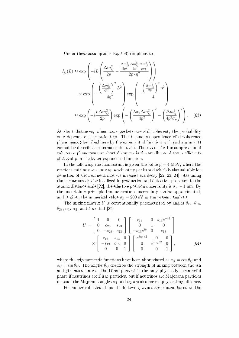
At short distances, when wave packets are still coherent, the probabilityonly depends on the ratio L/p. The L- and p-dependence of decoherencephenomena (described here by the exponential function with real argument)cannot be described in terms of the ratio. The reason for the suppression ofcoherence phenomena at short distances is the smallness of the coe�cientsof L and p in the latter exponential function.

In the following the momentum is given the value p = 4 MeV, where thereactor neutrino event rate approximately peaks and which is also suitable fordetection of electron neutrinos via inverse beta decay [22, 23, 24]. Assumingthat neutrinos can be localized in production and detection processes to theatomic distance scale [22], the e�ective position uncertainty is σx ∼ 1 nm. Bythe uncertainty principle the momentum uncertainty can be approximated,and is given the numerical value σp = 200 eV in the present analysis.

The mixing matrix U is conventionally parametrized by angles θ12, θ13,θ23, α1, α2, and δ so that [25]

U =

1 0 00 c23 s23

0 −s23 c23

c13 0 s13e−iδ

0 1 0−s13e

iδ 0 c13

×

c13 s13 0−s13 c13 0

0 0 1

eiα1/2 0 0

0 eiα2/2 00 0 1

, (64)

where the trigonometric functions have been abbreviated as cij = cos θij andsij = sin θij . The angles θij describe the strength of mixing between the ithand jth mass states. The Dirac phase δ is the only physically meaningfulphase if neutrinos are Dirac particles, but if neutrinos are Majorana particlesinstead, the Majorana angles α1 and α2 are also have a physical signi�cance.

For numerical calculations the following values are chosen, based on the

24

experimental limits [26]:

θ12 = 0.600967 (65a)

θ23 = 0.714450 (65b)

θ13 = 0.100000 (65c)

∆m221 = 7.59 · 10−5 eV2 (65d)

∆m232 = 243.00 · 10−5 eV2 (65e)

∆m231 = 250.59 · 10−5 eV2. (65f)

With these values one may estimate that

σp∆31p

≈ 2pσp∆m2

31

≈ 6 · 1011 � 1, (66)

and similarly the condition σE/∆31E � 1 of Section 4.3 is ful�lled, so thatthe massive neutrinos are indeed produced coherently.

5.2 Neutrino oscillations on di�erent scales

With the parameter values of the previous section, i.e. p = 4 MeV and mix-ing angles and squared mass di�erences given by Eqs. (65a)�(65f), transitionprobabilities may be given numerical values as a function of L. To get anestimate of length scales to investigate, the oscillation and coherence lengthsLoscij = 2p/∆m2

ij and Lcohij = (p/σp)(2p/∆m

2ij) are calculated:

Losc12 ≈ 20.806 km (67a)

Losc13 ≈ 0.63 km (67b)

Losc23 ≈ 0.65 km (67c)

Lcoh12 ≈ 416000 km (67d)

Lcoh13 ≈ 12600 km (67e)

Lcoh23 ≈ 13000 km. (67f)

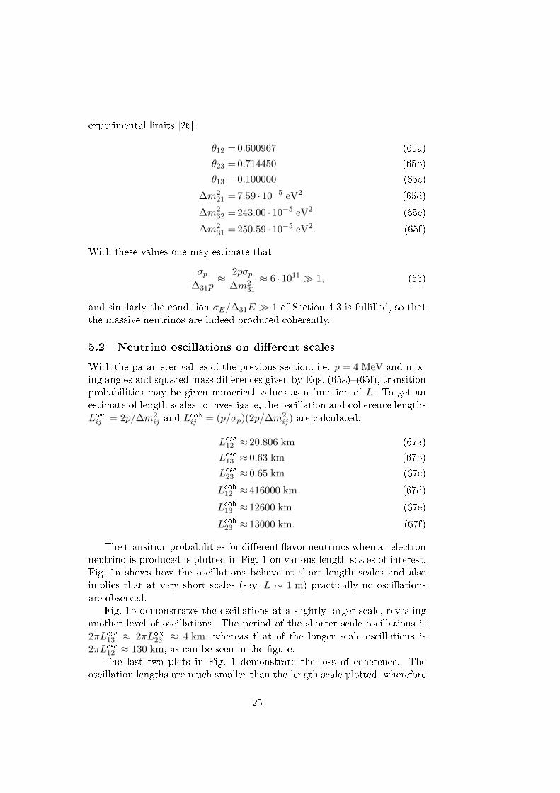
The transition probabilities for di�erent �avor neutrinos when an electronneutrino is produced is plotted in Fig. 1 on various length scales of interest.Fig. 1a shows how the oscillations behave at short length scales and alsoimplies that at very short scales (say, L ∼ 1 m) practically no oscillationsare observed.

Fig. 1b demonstrates the oscillations at a slightly larger scale, revealinganother level of oscillations. The period of the shorter scale oscillations is2πLosc

13 ≈ 2πLosc23 ≈ 4 km, whereas that of the longer scale oscillations is

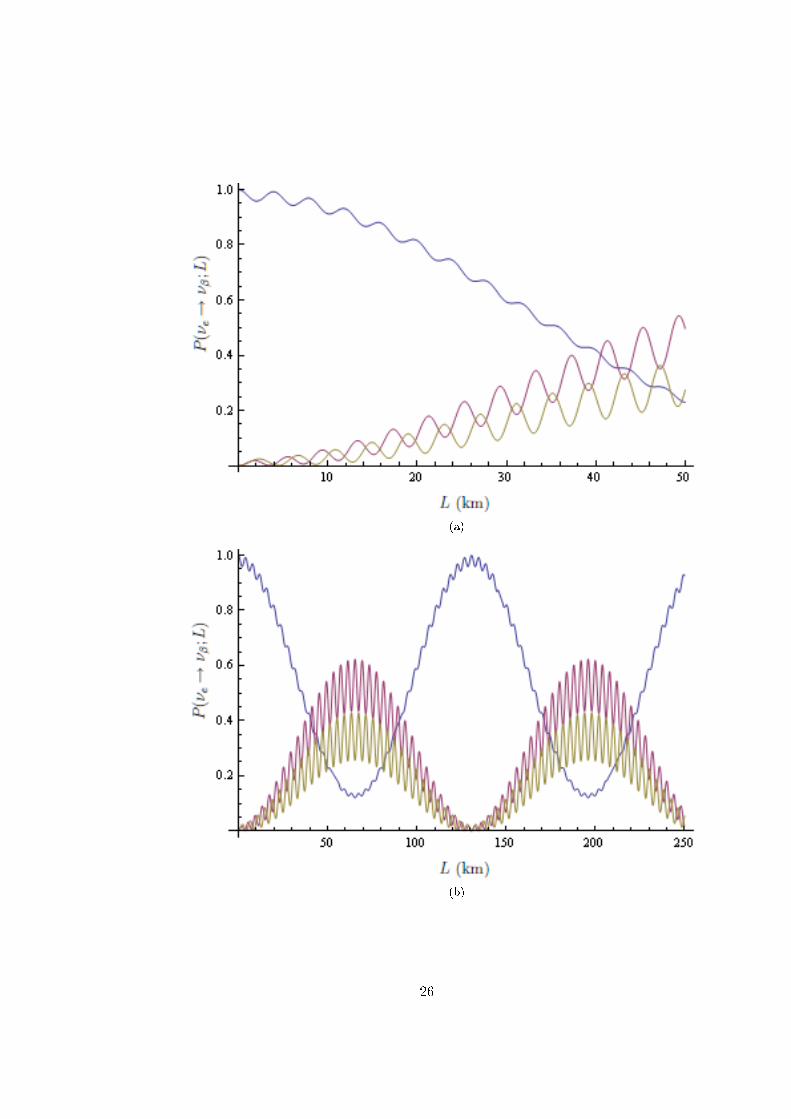
2πLosc12 ≈ 130 km, as can be seen in the �gure.The last two plots in Fig. 1 demonstrate the loss of coherence. The

oscillation lengths are much smaller than the length scale plotted, wherefore

25

(a)

(b)

Figure 1:

26

(c)

(d)

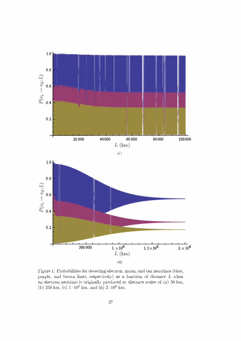
Figure 1: Probabilities for detecting electron, muon, and tau neutrinos (blue,purple, and brown lines, respectively) as a function of distance L whenan electron neutrino is originally produced at distance scales of (a) 50 km,(b) 250 km, (c) 1 · 105 km, and (d) 2 · 106 km.

27

the oscillation pattern is not visible. In Fig. 1c one may see a small decreasein the amplitude of probability oscillations caused by the wave packet of theheaviest massive neutrino ν3 being separated from those of the lighter ones(that is, Ii3(L)→ 0 in Eq. (63) for i = 1, 2).

A much more signi�cant change in the probability pattern is visible inFig. 1d. All wave packets are separated from each other, and all oscillationsare lost. The chance of �avor change remains, and is indeed signi�cant.

As Figs. 1c and 1d show, only the amplitudes of the oscillations in proba-bility are of interest at large distance scales, because the length scale greatlyexceeds that of the oscillations. Thus a simpler framework for the analysisof loss of coherence may be obtained through the analysis of envelope curvesto the �avor probability curves.

Because it was assumed that δ = α1 = α2 = 0, U is real, and thetransition probability given in Eqs. (39) and (63) becomes

P (να → νβ;L) =∑i,j

UαiUβiUαjUβjeiϕijCij

=∑i

(UαiUβi)2 + 2

∑i<j

UαiUβiUαjUβj cos(ϕij)Cij (68)

with abbreviating notations ϕij = −L∆m2ij/2p and

Cij = exp

−(Lσp∆m2ij

4p2

)2

−

(∆m2

ij

4p2σp

)2 . (69)

Using −1 ≤ cos(ϕij) ≤ 1 one immediately obtains upper and lower boundsfor the transition probabilities:

P up(να → νβ;L) =∑i

(UαiUβi)2 + 2

∑i<j

|UαiUβiUαjUβj |Cij , (70a)

P low(να → νβ;L) =∑i

(UαiUβi)2 − 2

∑i<j

|UαiUβiUαjUβj |Cij . (70b)

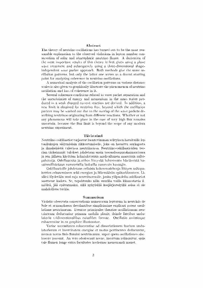
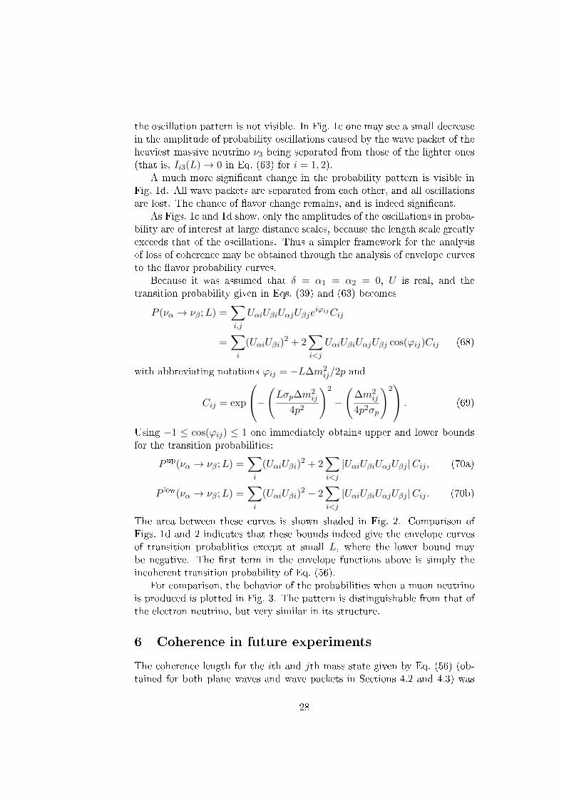
The area between these curves is shown shaded in Fig. 2. Comparison ofFigs. 1d and 2 indicates that these bounds indeed give the envelope curvesof transition probablities except at small L, where the lower bound maybe negative. The �rst term in the envelope functions above is simply theincoherent transition probability of Eq. (56).

For comparison, the behavior of the probabilities when a muon neutrinois produced is plotted in Fig. 3. The pattern is distinguishable from that ofthe electron neutrino, but very similar in its structure.

6 Coherence in future experiments

The coherence length for the ith and jth mass state given by Eq. (56) (ob-tained for both plane waves and wave packets in Sections 4.2 and 4.3) was

28

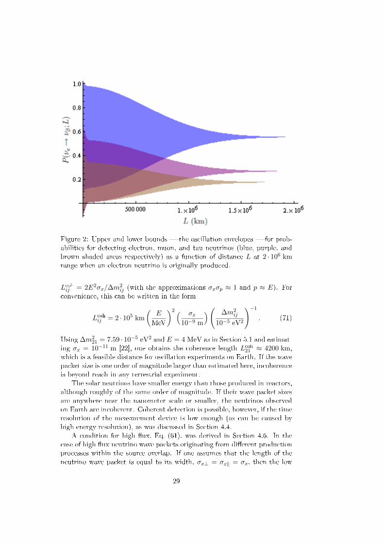
Figure 2: Upper and lower bounds � the oscillation envelopes � for prob-abilities for detecting electron, muon, and tau neutrinos (blue, purple, andbrown shaded areas respectively) as a function of distance L at 2 · 106 kmrange when an electron neutrino is originally produced.

Lcohij = 2E2σx/∆m

2ij (with the approximations σxσp ≈ 1 and p ≈ E). For

convenience, this can be written in the form

Lcohij = 2 · 105 km

(E

MeV

)2 ( σx10−9 m

)( ∆m2ij

10−5 eV2

)−1

. (71)

Using ∆m221 = 7.59 · 10−5 eV2 and E = 4 MeV as in Section 5.1 and estimat-

ing σx = 10−11 m [22], one obtains the coherence length Lcoh21 ≈ 4200 km,

which is a feasible distance for oscillation experiments on Earth. If the wavepacket size is one order of magnitude larger than estimated here, incoherenceis beyond reach in any terrestrial experiment.

The solar neutrinos have smaller energy than those produced in reactors,although roughly of the same order of magnitude. If their wave packet sizesare anywhere near the nanometer scale or smaller, the neutrinos observedon Earth are incoherent. Coherent detection is possible, however, if the timeresolution of the measurement device is low enough (as can be caused byhigh energy resolution), as was discussed in Section 4.4.

A condition for high �ux, Eq. (61), was derived in Section 4.6. In thecase of high �ux neutrino wave packets originating from di�erent productionprocesses within the source overlap. If one assumes that the length of theneutrino wave packet is equal to its width, σx⊥ = σx‖ = σx, then the low

29

(a)

(b)

Figure 3: Probabilities for detecting electron, muon, and tau neutrinos (blue,purple, and brown lines and shaded areas respectively) as a function of dis-tance L when a muon neutrino is originally produced at distance scales of(a) 50 km and (b) 2 · 106 km.

30

�ux condition may be written as σx � σmax, where the limit wave packetsize is σmax = (h/J)1/4. For high �ux phenomena to take place, the di�erentneutrinos should be produced coherently, which requires that the source is amacroscopic coherent quantum state. The Sun or a nuclear reactor do notmeet this condition, but their wave packet sizes are compared to the onerequired for high �ux to give an insight to the order of magnitude of thehigh �ux requirement.

For solar neutrinos the �ux is approximately J = 6 · 1010 cm−2s−1 [27],and the depth h of the source is estimated to be twice the radius of the solarcore, h = 0.5R� [28]. With these values one obtains σmax ≈ 4 m. Since thewave packet size is usually assumed to be at most in the nanometer scale,the solar neutrino �ux is low.

The �ux of neutrinos from a nuclear reactor are of the order of J =6 · 1012 cm−2s−1 [29], and a the reactor size is estimated to be h = 1 m.These estimates give the wave packet size the upper limit σmax ≈ 8 mm, sothe neutrinos are again safely in the low �ux regime.

The neutrino �uxes from these sources are so many orders of magnitudelower than would be required high �ux that it seems unlikely to be able toexperimentally verify the existence or nonexistence of any possible high �uxphenomena in near future. Whether or not such a high �ux would havean impact on neutrino oscillation can only be analyzed theoretically unlessunexpectedly great experimental advancements are made.

References

[1] J. Barranco, A. Bolanos, O. G. Miranda, C. A. Moura, and T. I.Rashba. Neutrino phenomenology and unparticle physics. ArXiv e-

prints, November 2009.

[2] J. N. Abdurashitov et al. Measurement of the solar neutrino capturerate by the Russian-American gallium solar neutrino experiment duringone half of the 22-year cycle of solar activity. J. Exp. Theor. Phys.,95:181�193, 2002.

[3] Francesco Vissani, Giulia Pagliaroli, and Francesco Lorenzo Villante. Onthe Goals of Neutrino Astronomy. Nuovo Cim., 032C:353�359, 2009.

[4] Gian Luigi Fogli, E. Lisi, A. Marrone, and G. Scioscia. Super-Kamiokande data and atmospheric neutrino decay. Phys. Rev.,D59:117303, 1999.

[5] Carlo Giunti. Neutrino Flavor States and the Quantum Theory of Neu-trino Oscillations. AIP Conf. Proc., 1026:3�19, 2008.

[6] S. M. Bilenky. Neutrinoless Double Beta-Decay. ArXiv e-prints, Jan-uary 2010.

31

[7] B. Kayser, F. Gibrat-Debu, and F. Perrier. The physics of massiveneutrinos. World Scienti�c Lecture Notes in Physics, 25, 1989.

[8] H. Fritzsch and Z.-Z. Xing. Mass and Flavor Mixing Schemes of Quarksand Leptons. Progress in Particle and Nuclear Physics, 45:1�81, Jan-uary 2000.

[9] C. Giunti. Fundamentals of Neutrino Physics and Astrophysics. Oxforduniversity press, 2007.

[10] Stephen T. Thornton and Jerry B. Marion. Classical dynamics of par-ticles and systems. Brooks/Cole, 2004.

[11] S. M. Bilenky, C. Giunti, J. A. Grifols, and E. Masso. Absolute Valuesof Neutrino Masses: Status and Prospects. Phys. Rept., 379:69�148,2003.

[12] Zhi-zhong Xing. Theoretical Overview of Neutrino Properties. Int. J.

Mod. Phys., A23:4255�4272, 2008.

[13] Yuval Grossman and Harry J. Lipkin. Flavor oscillations from a spatiallylocalized source: A simple general treatment. Phys. Rev., D55:2760�2767, 1997.

[14] Harry J. Lipkin. What is coherent in neutrino oscillations. Phys. Lett.,B579:355�360, 2004.

[15] Leo Stodolsky. The unnecessary wavepacket. Phys. Rev., D58:036006,1998.

[16] Yoshihiro Takeuchi, Yuichi Tazaki, S. Y. Tsai, and Takashi Yamazaki.How do neutrinos propagate? Wave packet treatment of neutrino oscil-lation. Prog. Theor. Phys., 105:471�482, 2001.

[17] E. K. Akhmedov and A. Y. Smirnov. Paradoxes of neutrino oscillations.Physics of Atomic Nuclei, 72:1363�1381, August 2009.

[18] C. Giunti. Coherence and wave packets in neutrino oscillations. Found.Phys. Lett., 17:103�124, 2004.

[19] Evgeny Kh. Akhmedov and Joachim Kopp. Neutrino oscillations: Quan-tum mechanics vs. quantum �eld theory. JHEP, 04:008, 2010.

[20] E. K. Akhmedov, J. Kopp, and M. Lindner. Oscillations of Mössbauerneutrinos. Journal of High Energy Physics, 5:5�+, May 2008.

[21] E. K. Akhmedov, J. Kopp, and M. Lindner. COMMENTS ANDREPLIES: Comment on 'Time-energy uncertainty relations for neutrinooscillations and the Mössbauer neutrino experiment'. Journal of PhysicsG Nuclear Physics, 36(7):078001�+, July 2009.

32

[22] Boris Kayser and Joachim Kopp. Testing the wave packet approach toneutrino oscillations in future experiments. ArXiv e-prints, 2010.

[23] F. Boehm. Reactor Neutrino Physics � An Update. ArXiv Nuclear

Experiment e-prints, June 1999.

[24] John G. Learned, Stephen T. Dye, and Sandip Pakvasa. Hanohano:A Deep ocean anti-neutrino detector for unique neutrino physics andgeophysics studies. ArXiv e-prints, 2007.

[25] Boris Kayser. Neutrino mass, mixing, and �avor change. ArXiv e-prints,2002.

[26] Particle Data Group. Leptons. http://pdg.lbl.gov/2009/tables/

rpp2009-sum-leptons.pdf, 2009 (accessed June 7, 2010).

[27] Carlos Pena-Garay and Aldo Serenelli. Solar neutrinos and the solarcomposition problem. 2008.

[28] Rafael A. Garcia, Sylvaine Turck-Chieze, Sebastian J. Jimenez-Reyes,Jerome Ballot, Pere L. Palle, Antonio E�-Darwich, Savita Mathur, andJanine Provost. Tracking Solar Gravity Modes: The Dynamics of theSolar Core. Science, 316(5831):1591�1593, 2007.

[29] M. Deniz et al. Measurement of Neutrino-Electron Scattering Cross-Section with a CsI(Tl) Scintillating Crystal Array at the Kuo-ShengNuclear Power Reactor. Phys. Rev., D81:072001, 2010.

33