Coherence and Decoherence in the Semiclassicalpropagation of the Wigner function

Disertación para optar al título deDoctor en Ciencias-Física de laUniversidad Nacional de ColombiaporLeonardo Augusto Pachón ContrerasBogotá, julio de 2010

Coherence and Decoherence in the Semiclassicalpropagation of the Wigner function

Leonardo Augusto Pachón ContrerasCódigo 183157Disertación para optar al título deDoctor en Ciencias-Física de laUniversidad Nacional de Colombia

Dirigido porProf. Thomas DittrichUniversidad Nacional de Colombia

Facultad de Ciencias

Departamento de Física

Bogotá, julio de 2010

Director: Prof. Dr. Thomas Dittrich

Jurado: Prof. Dr. Gert-Ludwig Ingold (Universität Augsburg, Germany)Jurado: Prof. Dr. John Henry Reina (Universidad del Valle, Colombia)Jurado: Prof. Dr. Karen Milena Fonseca (Universidad Nacional de Colombia, Colombia)

To my grandparents

María de los Ángelesand Gilberto (In Memoriam)

Acknowledgments

First of all, I would like to thank Prof. Thomas Dittrich for accepting me as a Ph.D.student and for giving me the opportunity to work in his group on a very interestingproject. I’m grateful to Prof. Dittrich because during the whole time of my Ph.D. hebehaved more as a collaborator than as a supervisor, collaborating with me even fromseveral remote places over the world. During this time I also I gained a lot from hisexperience, scientist intuition and passion for science. Last, but not least I enjoyed andlearnt a lot from our discussions about art, politics, science, history and cycling, thanksProfessor!

I thank Prof. Gert-Ludwing Ingold for giving me the opportunity to work in hisgroup during my internship in Augsburg and also for the warm hospitality which Ienjoyed there. During this time I really grew up as a scientist and also as a person. It isalso a pleasure to thank Carlos Viviescas, David Zueco, Raúl Vallejos and Juan DiegoUrbina for many discussion about a wide spectrum of subjects in physics, mathematicsand living.

I thank the members of the Chaos and Complexity group, present and former ones,for providing a stimulating and pleasant working atmosphere and for many encourag-ing discussions. In particular, I would like to thank, in the order I met them, FredyDubeibe, Edgar Gómez, Néstor Naranjo, Walter Acevedo, Arcesio Castañeda, EduardoZambrano, Arturo Argüelles, Ivonne Guevara and Oscar Barbosa for their friendshipand support during last years. I am indebted to Fredy for the careful and critical read-ing of this manuscript and to Edgar for sharing long nights, in opposite sides of theAtlantic ocean, propagating semiclassically Wigner functions.

I consider, it is time for me to apologize with Mi Muñeca because many times Ichanged her company for academic stuff, related and unrelated to this thesis. Mi Cielo,thanks for putting me up during last years and for being the friend, the girlfriend andthe wife which I ever need. I do not need to say that this thesis is for you because I knowyou feel it as yours. Thanks!

I thank my grandparents, María de los Ángeles (la nona Ángela) and Gilberto (elnono Gilberto R.I.P), and my parents, César Augusto and Norma Asunción, for theirunflagging support throughout my life. I also thank my brothers César Eduardo (Mo-chol), Leonela (Pempi), Luis Carlos (Lucho) and Gerdardo Andrés (Genaro), my cousinAndrés (El Calvo) and of course my nephew Juán Andrés (Juancho) for their supportivewords, this thesis is also for you!

i

I also thank the members of TP I and TP II in Augsburg University for the hospitalityand discussions about open quantum systems, statistical physics, art, food and living.In particular I thank Prof. Peter Talkner, Georg Reuther, (Gregorio el Terrible), EderSantana Annibale (The Brrrazilian), Michele Campisi, Cosimo Gorini, Yun Yun Lee(My beautiful girl), Alexey Ponomarev, Fei Zhan (The pasta-man) and Oleksandr Fialko.

During this time I also enjoyed hospitality and friendship of Luz Helena Sánchez,Óscar Flórez, Alexis Hernández (El veneco ...), Karen Rodriguez and Eufrasio Häh-nchen, Emilse Acevedo, María Espatolero and Lucía Zueco, Javier García, PaulinaLamas, Santiago Marroquín, Sinem Binicioglu Cetiner and Ender Cetiner, Igor andAlexey Protasov (The Brothers Karamazov). I specially thank Sinen and Ender for open-ing the door of their home in Augsubrg to Esmeralda and me. Paulina and Santiago,thanks for helping us with the moving from Augsburg.

I specially acknowledge to Julia Fernández, my mother-in-law, for her encouragingwords and wise advices. I thanks also the hospitality from Carolina Rodríguez, GermánOrlando, Violeta Gómez and from all the members of the Family Fernández.

Last, but not least, I render thanks to Family Valdés Solano and Family PachónRodriguez for supporting my application to a COLCIENCIAS’s scholarship. I am alsograteful to COLCIENCIAS and Universidad Nacional de Colombia for founding myposition at the Universidad Nacional de Colombia from September ’06 to June ’10 aswell as for the possibility to participate in conferences, workshops and internships inColombia, Brazil, France, Germany and United Kingdom.

Leonardo A. PachónBogotá, July 2010.

ii

Abstract

The present thesis addresses the subject of the semiclassical propagation of quantumcoherences in the framework of the Wigner formulation of quantum mechanics and isdivided into two main parts: i) the study of the evolution of quantum coherences inphase space and ii) the construction of a theory for non-Markovian dissipative systemsin phase space. In the first part work, we employed the semiclassical approximation de-veloped in [1] in order to study the propagation of superposition of coherent states andtunneling [2] and also to resolve the classical structures contributing to the semiclassi-cal spectral form factor [3,4]. In the second part, we translated the influence-functionaltheory [5] into phase-space language using the Marinov’s path-integrals [6]. This al-lowed us to construct the well-celebrated Caldeira-Leggett model [7, 8] in phase spaceand based on this result, we derived the non-Markovian propagating function of theWigner function and analyzed in detail the case of damped harmonic potentials [9,10].Subsequently, the semiclassical version of the propagating function is derived at threelevels: Ohmic dissipation at high temperatures, Ohmic dissipation and general non-Markovian dissipation [11].

iii

Notation

r,r Vectors in a 2 f -dimensional phase spaceR,R Vectors in a 2F-dimensional phase spaceR,R Vectors in a 2( f +F)-dimensional phase spaceA,M MatricesI Identity matrixJ Symplectic matrix∧ Symplectic product

H , DH Hilbert space and its corresponding dimension� Operator in Hilbert spaceρ Density matrix operator�W Weyl symbol of operator �

U , UW Unitary time-evolution operator and its associated Weyl symbolρW Wigner function assotiated to ρ

GW(r′′, t′′;r′, t′) Wigner propagator from r′ at t = t′ to r′′ at t = t′′

K (τ) Spectral form factortH Heisenberg timeD· Path integral along the trajectrory ·

I(ω) Spectral density of the bath modesγ(t),αR(t) Dissipative kernel and noise-correlation kernelJ(), JW() Propagating function and its phase-space analogousF [], FW[] Influence functional and its phase-space analogous

i, i∗ Imaginary unit and its complex conjugate

iv

List of Figures

2.1 Position and Wigner representation of the second excited state of the dou-ble well potential . . . . . . . . . . . . . . . . . . . . . . . . . . . . . . . . . . 7

3.1 Symplectic areas entering the semiclassical Wigner propagator, Eqs. (3.5,3.6), based on the van Vleck approximation . . . . . . . . . . . . . . . . . . 15

4.1 Time evolution of Schrödinger cat-states . . . . . . . . . . . . . . . . . . . . 214.2 Semiclassical description of coherent tunneling . . . . . . . . . . . . . . . 234.3 Autocorrelation function of a Gaussian initial state in a quartic double

well potential . . . . . . . . . . . . . . . . . . . . . . . . . . . . . . . . . . . . 23

5.1 Schematic plot of a set of periodic points of a symplectic map with theirmidpoints and surface formed by midpoints of a fictitious continuous pe-riodic orbit that is not circularly symmetric nor confined to a plane . . . 29

5.2 Geometrical picture of the classical cat map . . . . . . . . . . . . . . . . . . 305.3 Diagonal Wigner propagator for the quantized Arnol’d cat map. . . . . . . 315.4 Geometrical picture of the classical baker map . . . . . . . . . . . . . . . . 325.5 Diagonal Wigner propagator for the quantized baker map . . . . . . . . . 325.6 Geometrical picture of the classical D-transformation . . . . . . . . . . . . 335.7 Diagonal Wigner propagator for the D-transformation . . . . . . . . . . . 335.8 Diagonal Wigner propagator for the kicker rotor . . . . . . . . . . . . . . . 345.9 Diagonal Wigner for the quartic oscillator and midpoints manifolds . . . 365.10 Diagonal Wigner and Liouville propagators for the harmonically driven

quartic oscillator . . . . . . . . . . . . . . . . . . . . . . . . . . . . . . . . . . 37

6.1 The time evolution of a pair of phase-space trajectories in the presence ofa damped harmonic oscillator . . . . . . . . . . . . . . . . . . . . . . . . . . 45

6.2 Isosurface of the time-dependent Wigner propagating function of a har-monic oscillator . . . . . . . . . . . . . . . . . . . . . . . . . . . . . . . . . . . 46

7.1 Wigner propagating-function of a Morse oscillator . . . . . . . . . . . . . . 63

v

A.1 Schematic description of the chord rule . . . . . . . . . . . . . . . . . . . . 67

C.1 Preparation of initial points for the propagation algorithm for smoothinitial distributions . . . . . . . . . . . . . . . . . . . . . . . . . . . . . . . . 73

E.1 Integration contour in the complex time plane z = s+ iτ along which theexponent of the influence functional is calculated . . . . . . . . . . . . . . 78

vi

Contents

Acknowledgments i

Abstract iii

Notation iv

List of Figures vi

1 Introduction 1

2 Quantum Mechanics in Phase Space 4

2.1 The Weyl Transform . . . . . . . . . . . . . . . . . . . . . . . . . . . . . . . 42.2 The Wigner Function . . . . . . . . . . . . . . . . . . . . . . . . . . . . . . . 5

2.2.1 Properties of the Wigner Function . . . . . . . . . . . . . . . . . . . 62.2.2 Time Evolution of the Wigner Function . . . . . . . . . . . . . . . . 6

2.3 Quantum Dynamics in Phase Space . . . . . . . . . . . . . . . . . . . . . . 72.3.1 Properties of the Wigner Propagator . . . . . . . . . . . . . . . . . . 82.3.2 Alternative Expressions for the Wigner Propagator . . . . . . . . . 9

2.4 Wigner Function for Discrete Phase-Spaces . . . . . . . . . . . . . . . . . . 112.4.1 Wigner Function and Wigner Propagator over a Torus . . . . . . . 122.4.2 Wigner Function and Wigner Propagator over a Cylinder . . . . . 12

3 Semiclassical Wigner Propagator 14

3.1 From Weyl Propagator to Semiclassical Wigner Propagator . . . . . . . . 143.2 From Van Vleck Propagator to Semiclassical Wigner Propagator . . . . . 173.3 From Phase-Space Path-Integrals to Semiclassical Wigner Propagator . 183.4 From Liouville-Propagator Eigenfunctions to Semiclassical Wigner Prop-

agator . . . . . . . . . . . . . . . . . . . . . . . . . . . . . . . . . . . . . . . . 19

vii

4 Semiclassical Description of Quantum Coherences in Phase Space 20

4.1 Semiclassical Propagation of Schrödinger’s Cat-States . . . . . . . . . . . 204.2 Semiclassical Description of Tunneling . . . . . . . . . . . . . . . . . . . . . 224.3 Summary . . . . . . . . . . . . . . . . . . . . . . . . . . . . . . . . . . . . . . 24

5 Quantum Coherences and Semiclassical Spectral Statistics 25

5.1 Classical and Quantum Return-Probabilities . . . . . . . . . . . . . . . . . 265.2 Form Factor and Diagonal Propagator . . . . . . . . . . . . . . . . . . . . . 285.3 Example i: Discrete Time Dynamics . . . . . . . . . . . . . . . . . . . . . . 29

5.3.1 The Arnol’d Cat-Map . . . . . . . . . . . . . . . . . . . . . . . . . . . 295.3.2 The Baker Map . . . . . . . . . . . . . . . . . . . . . . . . . . . . . . . 305.3.3 The D-Transformation . . . . . . . . . . . . . . . . . . . . . . . . . . 325.3.4 The Kicked Rotor . . . . . . . . . . . . . . . . . . . . . . . . . . . . . 33

5.4 Example ii: Continuous Time Dynamics . . . . . . . . . . . . . . . . . . . . 345.4.1 The Quartic Oscillator . . . . . . . . . . . . . . . . . . . . . . . . . . 355.4.2 The Harmonically Driven Quartic Oscillator . . . . . . . . . . . . . 36

5.5 Summary . . . . . . . . . . . . . . . . . . . . . . . . . . . . . . . . . . . . . . 37

6 Open Quantum Systems in Configuration Space 39

6.1 Feynman and Vernon Theory . . . . . . . . . . . . . . . . . . . . . . . . . . . 396.2 Quantum Damped Harmonic Oscillator . . . . . . . . . . . . . . . . . . . . 41

6.2.1 Damped Harmonic Oscillator in Phase Space . . . . . . . . . . . . 43

7 Open Quantum Systems in Phase Space 47

7.1 Feynman and Vernon Theory in Phase Space . . . . . . . . . . . . . . . . . 477.2 Ullersma-Caldeira-Leggett Model in Phase Space . . . . . . . . . . . . . . 497.3 Semiclassical Approximation . . . . . . . . . . . . . . . . . . . . . . . . . . . 50

7.3.1 Semiclassical Approximation: Langevin Trajectories Approach . . 507.3.2 Semiclassical Approximation: Reduced density matrix approach . 537.3.3 Numerical Results for non-Harmonic Potentials . . . . . . . . . . . 62

7.4 Summary . . . . . . . . . . . . . . . . . . . . . . . . . . . . . . . . . . . . . . 63

8 Conclusions and Outlook 64

A Weyl Propagator from Van Vleck Propagator 66

B Split-Operator Method for the Wigner Propagator 68

C Numerical Calculation of The Semiclassical Wigner Propagator 71

C.1 Van Vleck-Based Semiclassical Approximation . . . . . . . . . . . . . . . . 71C.2 Propagating Smooth Localized Initial States: Towards Monte Carlo Algo-

rithms . . . . . . . . . . . . . . . . . . . . . . . . . . . . . . . . . . . . . . . . 72

D Wigner Propagator Near Periodic Orbits 74

E Influence-Functional Theory for non-Factorizing Initial Conditions 77

E.1 Propagating Function of the Wigner Function . . . . . . . . . . . . . . . . 79

viii

F Ullersma-Caldeira-Leggett Model in Phase Space 80

Bibliography 84

ix

CHAPTER 1

Introduction

The understanding of the quantum-classical transition undoubtedly constitutes one ofthe more interesting problems in physics and it has attained the attention since theestablishment of quantum theory in last century [12–14]. It has persuaded the longevolution on our concept of what is quantum and to what extent it is required to explainobservations in nature.

By contrast to the beginning of the quantum theory, when the reduction postulateclearly separated between quantum microscopic entities and classical macroscopic mea-suring apparatuses [14], our present conception of the quantum realm makes that weconceive the border between the classical and quantum worlds more diffuse and intrigu-ing than one century ago. This kind of “regression” has been supported by quantumphenomena such as superconductivity [15], coherent superposition in Bose-Einsteincondensates [16], together with interference fringes of very massive molecules [17]and more recently by the proposals to create superpositions of dielectric bodies, suchas viruses up to micron size [18] and to entangle quantum oscillators, even, at roomtemperature [10].

The first attempt towards the identification of quantum contributions to the dynam-ics of physical systems in terms of classical entities was the 1926 WKB approximation(Wentzel [19], Kramers [20], and Brillouin [21]), which recast the wavefunction as anexponential of an evolving Lagrangian manifold [22]. The second successful approachwas the 1928 semiclassical approximation of the unitary time-evolution operator de-rived by van Vleck [23] with subsequent contributions by Gutzwiller [24]. This quan-tity is arguably one of the most fundamental objects of semiclassical theory because itconstitutes, e.g., the starting point for the derivation of the celebrated Gutzwiller traceformula [25] and also for the semiclassical reaction rate theory [26,27].

Before the establishment of the KAM theorem (Kolmogorov [28, 29], Arnold [30]and Moser [31]) in the 50’s, semiclassical dynamics of regular and chaotic systemswas treated without no difference. However, after the KAM theorem, chaotic systemsbegan to be widely appreciated [32] and the search of chaos in the time development

1

of quantum systems started. However, such attempts failed and it was found thatafter a long enough time the chaos of classical mechanics is always suppressed byquantum mechanics [33]. Although, there is still no general analytical theory of thissuppression, there are several qualitative and semiquantitative explanations such asthat driven quantum systems absorb energy more slowly than their chaotic classicalcounterparts [33], that bound systems have discrete energy levels, that the Schrödingerequation is linear or that Planck’s constant ~ smooths away classical phase-space finestructure [34–36] or replaces it, effectively, by a discrete lattice [37].

In this way, we can realize that the transition from quantum to classical realms ismore thought-provoking when the classical systems is chaotic. This was the origin oflot of interest and a huge number of related works in the 70’s and 80’s. Probably thetwo more important discoveries in the field at that time were:

• The discovery of evidence that the spectrum of quantum systems bears infor-mation on the corresponding classical dynamics, in particular on manifolds in-variant under time evolution: periodic orbits. The establishment of this directconnection between the quantum energy spectrum of bound motion and periodicorbits is based on the remarkable works by Gutzwiller [24, 25, 38, 39] with im-portant subsequence contributions by Balian and Bloch [40–43] and Berry andTabor [44–46].

• The discovery that energy eigenfunctions are influenced not only by the energysurface [47–49], which is the generic invariant manifold, but by individual closedorbits, which are invariant sets of zero measure. This picture emerged from nu-merical and theoretical evidence embodied in the seminal works by Heller [50,51].It is worth mentioning that the imprints of closed orbits persist up through thou-sands of states and probably survive into the classical limit. Heller calls theseimprints scars [52] as they allowed, for the first time, to directly visualize theimpact of classical invariant manifolds on quantum mechanical distributions de-fined on configuration [50,51] or phase space [53].

The suppression of chaos at the quantum level and the suppression of quantumbehavior at the classical level are currently understood, partially [54], in terms of thepresence of quantum coherences and the phenomenon of decoherence [12, 13], respec-tively. It implies that as soon as the system interacts and evolves in the presence ofa surrounding environment, “quantumness” is faded out into the degree of freedom ofthe environment. In this sense, a semiclassical treatment explaining how, in this tran-sition region, quantum effects appear or disappear would be desirable. However, thesemiclassical description of quantum coherences certainly is far from being a trivialtask because “quantumness” is typically encoded in phenomena of infinity order in thePlanck constant such as tunneling [55] or entanglement [56] and since semiclassicaltheories are typically of second order in ~, then the description of such phenomenarepresents a big challenge for semiclassical approximations. In Chap. 4 we presenta discussion about quantum coherences in semiclassical terms under the light of re-cent progress in the semiclassical propagation of quantum states [1,57] and show thatwithin semiclassical approximations [1] is possible to provide a successful description

2

of these pure quantum correlations [2]. On the other hand, in Chap. 5 we show thatthe same approach can be used to resolve the classical invariant manifold contributingto the spectral correlation of classical integrable and chaotic systems [3, 4]. Addition-ally, we discover scars, which in contrast to the usual ones [50, 51, 53], ours are notrestricted to the uncertainty principle.

On the other hand, the evolution of quantum systems in the presence of an envi-ronment is clearly more demanding than the unitary cases and there is not a uniqueway of introducing the effect of a thermal bath in the system under study [58]. Thefirst approaches were based on phenomenological descriptions [59] and were plaguedof fundamental problems such as the contraction of unitary cells in the quantum phasespace [58]. The most successful approach was developed by Feynman and Vernon [5]and it is known as the influence-functional theory. This approach condenses the influ-ence of the environment in a single object given by a path-integral expression and thesubsequent trace over the freedoms of the thermal bath (see Chap. 6). The first success-ful description of a physical system within this approach was developed by Ullersmain a series of three papers [60–62], the key ingredient was the assumption of the bathas a collection of harmonic oscillators [60]. Some years later, the same model was usedby Caldeira and Leggett to study quantum tunneling [7] (see [8] for a detailed accountof the calculation).

The semiclassical description of open quantum systems (systems in contact with athermal bath) has deserved attention during past years [63–66], and in present yearsthere have been a lot of works in the field [67–72]. However, most of current develop-ments are not formally derived or are not completely consistent or introduce additionalapproximations, such as the Markovian approximation [73,74].

Motivated by lack of a fully consistent and general semiclassical theory for dissipa-tive systems and by the transparent structure of [1] and its high performance exploredin chapters 4 and 5, we elaborate in Chap. 7 the dissipative version of this approach fornon-Markovian dissipative systems. This result opens the possibility for a formal andconsistent study of the semiclassical spectral-statistics of dissipative systems [75, 76],the study of reaction theory far from equilibrium and the description of decoherenteffects in terms of classical manifolds. Moreover, it could give some insights into theevolution of entanglement in semiclassical terms [77].

With this work we pretend to contribute to the understanding of how nature be-haves at the quantum level in terms of classical entities and provide accurate andefficient algorithms to the propagation of quantum systems. Finally, we concludewith the hope that the results presented here, provide powerful computational toolsand an insightful description and of interesting phenomena such as photosynthesis[78, 79], other biological processes [80] and implementations of quantum computationin “medium-size” molecules [81,82].

3

CHAPTER 2

Quantum Mechanics in Phase Space

A classical system S with position coordinates q = (q1, q2, · · · , q f ) and conjugate mo-mentum coordinates p = (p1, p2, · · · , p f ) can be described by a probability functionf (r) = f (p,q) in the 2 f -dimensional phase space. In such a way, f (p,q)df pdf q de-notes the probability that the system be in a volume element df pdf q around r. In thequantum-mechanically description of S, the phase-space coordinates cannot be definedsimultaneously, in that sense the concept of probability function cannot be extended toquantum mechanics. However, there is possible to construct quasi-probability distri-butions [83], which in conceptual and operational terms are equivalent to the classicalprobability functions.

Among those quasi-probability functions in phase space, the Wigner function [84]has been the most used in most of the branches of the non-relativistic quantum me-chanics [83], e.g., in quantum optics and in statistical quantum mechanics, becauseit allows a treatment of quantum mechanics in complete analogy with the classicalstatistical mechanics. In particular, the possibility of defining and establishing moredirect relations and analogies between quantum and classical mechanics has given tothe Wigner function a special place in the “quantum chaos community” [48,85,86].

In this chapter, we briefly introduce the formulation of quantum mechanics in phasespace by using the Wigner function, it will allow us to fix the notation and to introducesome of the basic ideas for this thesis. For a more detailed and extended presentation,we refer the reader to the Hillary’s et al. report [83] and to the report by Ozorio deAlmeida [86].

2.1 The Weyl Transform

The Weyl symbol AW (p, q) of an arbitrary operator A( p, q) can be defined as

AW(p, q)= TW[

A]

(p, q)=Tr[

A( p, q)d( p, q)]

, (2.1)

4

where the operator d(p, q) is defined in terms of the displacement operator T(u,v) (see[86] for a definition and some properties of the displacement operator)

d(p, q) =∫

dudv

2π~exp

{

i

~(up+vq)

}

T(−u,−v). (2.2)

AW(p, q) is completely analogous to A( p, q) in the sense that

A( p, q)= (2π~)−1∫

dpdqAW(p, q)d(p, q), (2.3)

with normal ordering [83, 87]. Since Tr[

d(p, q)]

= 1, then the trace of an operator inphase space can be calculated as an average of the corresponding Weyl symbol over thewhole phase space, i.e.

Tr[

A]

= (2π~)−1∫

dpdqAW(p, q). (2.4)

For an f -dimensional system, the Weyl symbol of the operator A( p, q), can be expressedas

AW(p,q) =∫

df uexp{

− i

~p ·u

}

⟨

q+ u

2

∣

∣A∣

∣q− u

2

⟩

, (2.5)

where we have evaluated the trace operation in (2.1) in terms of eigenstates of the posi-tion operator, q|q1⟩ =q1|q1⟩. A similar expression can be derived in terms eigenstatesof the momentum operator.

2.2 The Wigner Function

The quantum description of a system S, in the Wigner’s formulation, is not based onthe state vector |ψ⟩ but on the density matrix ρS, which contains the relevant physicalinformation of the system under study and is the main object of the statistical quantummechanics. The density operator can be expressed as a superposition of pure states

ρS =∑

jp j

∣

∣ψ j⟩⟨ψ j∣

∣ , (2.6)

where p j can be understood as the probability that the system be in the state∣

∣ψ j⟩. Itmeans that {0 ≤ p j ≤ 1,∀ j},

∑

j p j = 1 and∑

j p2j ≤ 1, where the equality holds for pure

states. If we assume that ρS is known, then the expectation value of the operator O attime t is defined as ⟨O(t)⟩ =Tr

[

OρS(t)]

.The Wigner function, ρW(p,q), is defined as the Weyl transform of ρS/(2π~) f , i.e.

ρW(p,q)= TW

[

ρS

(2π~) f

]

(p,q)=∫

df uexp{

−i

~p ·u

}⟨

q+u

2

∣

∣

∣

∣

ρS

(2π~) f

∣

∣

∣

∣

q−u

2

⟩

. (2.7)

5

If the density matrix correspond to a pure state, ρS = |ψ⟩⟨ψ|, then

ρW(p,q)=∫

df uexp{

−i

~p ·u

}

⟨q+u

2

∣

∣ψ⟩⟨ψ∣

∣q−u

2⟩. (2.8)

In this way, the Wigner function at (p,q) corresponds to the Fourier transform of theproduct of the wave function reflected at −2q times the complex conjugate of this re-flected at 2q.

2.2.1 Properties of the Wigner Function

From the definition of the Wigner function given in (2.7) it is possible to show that

• The Hermiticity of the density matrix implies that Wigner function is real.

• From (2.7) and assuming that Tr[ρ] = 1, then∫

df pdf qρW(p,q) = Tr[ρW] = 1,which implies that the Wigner function is normalized. It is worth mentioningthat despite that the Wigner function can take negative values in some regionsof phase space, the measure of those regions is such that the integral over thewhole phase space is positive.

• The probability in position (or momentum) representation |ψ(q)|2(

|ψ(p)|2)

, arecorrectly given by

∫

df pρW(p,q),(∫

df qρW(p,q))

. Even, it can be shown thatthe Wigner function is the only quasi-probability distribution which satisfies thisstatement in a general way, i.e., it generates the correct marginal probabilityalong any direction between q and p-axis in phase space [88].

• If ρ corresponds to a mixed state, then∫

df pdf q|ρW(p,q)|2 ≤ 1(2π~) f . The equality

stands for pure states.

In order to exemplify Wigner’s formulation, in Fig. 2.1 we depict the second ⟨q|2⟩and third ⟨q|3⟩ excited state, the second tunneling doublet (cf. Sec. 4.2), of the doublewell potential (4.8) in position and in Wigner representation. Although the differencebetween ⟨q|2⟩ (Fig. 2.1a) and ⟨q|2⟩ (Fig. 2.1b) is noticeable in position representation,it is interesting to note that in phase space the only difference between ρW,2 (Fig. 2.1c)and ρW,3 (Fig. 2.1d) is the phase of the oscillatory central-pattern, for ρW,2 this ispositive at p = 0 while this is negative for ρW,3.

In the following, we address the issue of the propagation of the Wigner function interms of the propagator of the Wigner function and list some of its properties.

2.2.2 Time Evolution of the Wigner Function

For one dimensional systems and assuming H(p, q) = p2

2m +V (q), the time evolution ofthe Wigner function is generally expressed by the differential equation [83]

∂ρW

∂t=−∂H

∂p

∂ρW

∂q+ ∂H

∂q

∂ρW

∂p+

∑

n>2(odd)

1

n!

(

~

2i

)n−1 ∂nH

∂qn

∂nρW

∂pn,

6

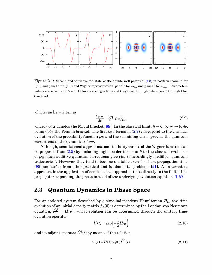
Figure 2.1: Second and third excited state of the double well potential (4.8) in position (panel a for

⟨q|2⟩ and panel c for ⟨q|3⟩) and Wigner representation (panel c for ρW,2 and panel d for ρW,3). Parameters

values are m = 1 and ∆ = 1. Color code ranges from red (negative) through white (zero) through blue

(positive).

which can be written as∂ρW

∂t=

{

H,ρW}

M , (2.9)

where {·, ·}M denotes the Moyal bracket [89]. In the classical limit, ~→ 0, {·, ·}M → {·, ·}P,being {·, ·}P the Poisson bracket. The first two terms in (2.9) correspond to the classicalevolution of the probability function ρW and the remaining terms provide the quantumcorrections to the dynamics of ρW.

Although, semiclassical approximations to the dynamics of the Wigner function canbe proposed from (2.9) by including higher-order terms in ~ to the classical evolutionof ρW, such additive quantum corrections give rise to accordingly modified “quantumtrajectories”. However, they tend to become unstable even for short propagation time[90] and suffer from other practical and fundamental problems [91]. An alternativeapproach, is the application of semiclassical approximations directly to the finite-timepropagator, expanding the phase instead of the underlying evolution equation [1,57].

2.3 Quantum Dynamics in Phase Space

For an isolated system described by a time-independent Hamiltonian HS, the timeevolution of an initial density matrix ρS(0) is determined by the Landau-von Neumannequation, idρ

dt = [H, ρ], whose solution can be determined through the unitary time-evolution operator

U(t)= exp(

− i

~HSt

)

(2.10)

and its adjoint operator U†(t) by means of the relation

ρS(t)= U(t)ρS(0)U†(t). (2.11)

7

In position representation, this expression turns into

ρS(q′′+, q′′

−, t)=∫

dq′+dq′

−J(q′′+, q′′

−, t; q′+, q′

−,0)ρS(q′+, q′

−,0) , (2.12)

whereJ(q′′

+, q′′−, t; q′

+, q′−,0)=U(q′′

+, q′+, t)U∗(q′

−, q′′−, t), (2.13)

with U(q′′±, q′

±, t)= ⟨q′′±|U(t)|q′

±⟩ and ρS(q+, q−)= ⟨q+|ρS|q−⟩. If ρS(q′′+, q′′

−, t) [ρS(q′+, q′

−,0)]is transformed to phase space, it is described by the Wigner function ρW(r′′, t) [ρW(r′,0)]and the time evolution equation (2.11) reads

ρW(r′′, t)=∫

dr′GW(r′′, t;r′,0)ρW(r′,0), (2.14)

where GW(r′′, t;r′,0) is the propagator of the Wigner functions given by [1,6]

GW(r′′, t;r′,0)≡ 1

(2π~)2

∫

dreir∧(r′′−r′)/~UW (r+)U∗W (r−) , (2.15)

with r±(r′′+ r′± r)/2. In (2.15), r and r denote generic points in phase space; ri ∧ r j,

the symplectic product rTi Jr j, being J=

(

0 I

−I 0

)

the symplectic matrix and UW(r) the

Weyl transform of the evolution operator.

2.3.1 Properties of the Wigner Propagator

Due to the close relation between the Weyl propagator and the Wigner propagator, itis not surprising that the properties of the Wigner propagator depend directly on theproperties of the time-evolution operator U. In particular, the anti-unitarity of U istranslated to the Weyl propagator as U∗

W(r, t)=UW(r,−t)=U−1W (r, t).

• Since at t = 0, U(0)= 1, then UW(r,0)= 1, from here follows immediately that

G(r′′,0;r′,0)= δ(r′′−r′),

which implies that the Wigner propagator is not restricted by the uncertaintyprinciple. This fact allows a clear and conceptually simple study of the quantum-classical transition [4].

• From the composition law for the unitary time-evolution operator we can showthat

GW(r′′, t;r′,0)=∫

d2 f r′′′GW(r′′, t;r′′′, t′′′)GW(r′′′, t′′′;r′,0), (2.16)

i.e., the propagator satisfies a Chapmann-Kolmogorov type equation.

• From (2.15), from the anti-unitarity of U and assuming that the quantum systemis homogeneous in time, we have that

GW(r′′, t;r′,0)=GW(r′,−t;r′′,0)=GW(r′,0;r′′, t).

8

In this way, for autonomous Hamiltonian systems, the Wigner propagator induces adynamical group parameterized by t. Other properties of GW(r′′, t;r′,0) are

• Since the Wigner function is real, then G(r′′,0;r′,0)∈Re

• The propagator of the Wigner function is an orthogonal operator, i.e.∫

d2 f r′′′G(r′′, t;r′,0)G(r′′′, t;r′,0)= δ(r′′−r′).

2.3.2 Alternative Expressions for the Wigner Propagator

Although expression (2.15) admits a clear interpretation in terms of two counter-pro-pagating propagators, its numerical evaluation is highly demanding and therefore ad-ditional expressions with an accessible numerical implementation are desirable. Inthe following, we present three different, yet equivalent expressions for the Wignerpropagator.

Wigner Propagator from Eigenstates of H

Since the eigenbasis {|n j⟩} of the Hamiltonian H is also an eigenbasis for exp(

− i~

Ht)

,then it is natural to represent the unitary time-evolution operator in terms of the eigen-basis of H and calculate the Weyl propagator in this representation,

UW(r, t)=∫

df u exp(

−i

~p ·u

)

∑

n,n′⟨q+

u

2|n′⟩⟨n′|exp

(

−i

~Ht

)

|n⟩⟨n|q−u

2⟩

= (2π~) f∑

nexp

(

− i

~Ent

)

ρW,nn(r), (2.17)

where

ρW,nn(p,q)=1

(2π~) f

∫

df uexp(

−i

~p ·u

)

⟨q+u

2|n⟩⟨n|q−

u

2⟩, (2.18)

denotes the Wigner function of the state |n⟩. Inserting (2.17) in (??) we get

GW(r′′, t;r′,0)=∑

n,m

∫

d2 f r exp(

i

~r∧ (r′′−r′)

)

exp(

−iEn −Em

~t)

×∫

df u+exp(

− i

~p+ ·u+

)

⟨q++u+2

|n⟩⟨n|q+−u+2

⟩ (2.19)

×∫

df u−exp(

− i

~p− ·u−

)

⟨q−+u−2

|m⟩⟨m| q−− u−2

⟩

or

GW(r′′, t;r′,0)=

(2π~)2 f∑

n,m

∫

d2 f r exp(

i

~r∧ (r′′−r′)

)

exp(

−iEn −Em

~t)

ρW,nn(r+)ρW,mm(r−)

(2.20)

9

where r± = r′′+r′±r2 . After some algebraic manipulations, it is possible to show that

GW(r′′, t;r′,0)= (2π~) f∑

n,mexp

(

−iEn −Em

~t)

ρW,nm(r′′)ρW,mn(r′), (2.21)

being

ρW,nm(p,q)=1

(2π~) f

∫

df uexp(

−i

~p ·u

)

⟨q+u

2|n⟩⟨m|q−

u

2⟩, (2.22)

the mixed Wigner function corresponding to |n⟩⟨m|.

Wigner Propagator from the Unitary Time-Evolution Propagator

In order to establish a more direct link between the Wigner propagator and the unitarytime-evolution propagator, we can insert the formal expression for UW(r) in terms of Uin (2.19) this leaves with the following expression for the Wigner propagator

GW(r′′, t;r′,0)=2 f

h f

∫

df q′∫

df q′′exp{

i

~(p′ · q′−p′′ · q′′)

}

×U∗(

q′′− q′′

2, t;q′− q′

2,0

)

U(

q′′+ q′′

2, t;q′+ q′

2,0

)

.

(2.23)

This expression is the most convenient route in terms of numerical implementations be-cause U(q′′,q′) can be calculated by using a split operator method and then GW(r′, t;r,0)is evaluated by using fast Fourier transforms [92]. In Appendix B we provide a descrip-tion of this algorithm. It is illustrative to analyze (2.23) and (2.13) together because wecan identify the Wigner propagator as a “double fourier transform” of the propagatorof the density matrix J(q′′

+,q′′−, t;q′

+,q′−,0) along the difference coordinate q′′ =q′′

+−q′′−

and q′ =q′+−q′

− as

GW(r′′, t;r′,0)= 2 f

h f

∫

df q′∫

df q′′ei~

(p′·q′−p′′·q′′)J(

q′′+ q′′

2,q′′− q′′

2t;q′+ q′

2,q′− q′

2,0

)

,

(2.24)

where q′′ = (q′′+−q′′

−)/2 and q′ = (q′+−q′

−)/2. Expression (2.24) is also valid in the dissi-pative case as we can see in Sec. 6.2.1 (see Eq. 6.23) or in [9].

Wigner Propagator from Path Integral in Phase Space

In order to derive a path integral expression for the Wigner propagator, we follow thework by Marinov [6] and divide the time interval (t′, t′′), á la Feynman [93], in N smalltime steps ∆t = (t′′− t′)/N. For small ∆t, the Weyl transform of the unitary evolutionoperator reads UW(r,∆t)∼ exp

(

− i~

HW(r)∆t)

, where HW(r) denotes the Weyl transformof the Hamiltonian operator [91]. Replacing this expression in 2.15, we obtain that forshort times the Wigner propagator is given by

GW(rn,rn−1)=1

(2π~) f

∫

d2 f rn exp(

i

~φn

)

, (2.25)

10

where we have defined φn ≡ ∆rn ∧ rn +(

HW

(

rn + rn2

)

−HW

(

rn − rn2

))

∆t , with ∆rn ≡rn −rn−1 and rn ≡ rn+rn−1

2 . Since the propagator satisfies a Chapman-Kolmogorov typeequation (see Eq. (2.16)), we can derive the propagator for finite times,

GW(r,r0)= limN→∞

N−1∏

n=1

[∫

d2 f rn

] N∏

n=1

[∫

d2 f rn

(2π~) f

]

exp

(

i

~

N∑

n=1φn

)

. (2.26)

In the continuous limit, the phase in (2.26) acquires the form of an integral functionalaction

N∑

n=1φn → S[{r}, {r}, t]≡

∫t

0

[

r∧ r+HW(r+ 1

2r)−HW(r− 1

2r)

]

dt′, (2.27)

where r(t′) is a trajectory in phase space with initial point r(0) = r′ and final pointr(t)= r′′, r= dr/dt and r can be considered as a fluctuation without restrictions aroundr(t′). So, finally we have that the Wigner propagator can be written as,

GW(r,r0)= 1

(2π~) f

∫

D2 f r

∫

D2 f r exp

(

i

~S[{r}, {r}, t]

)

, (2.28)

where D2 f r and D

2 f r denote each one a set of infinity measures in phase space [6]. Wemake use of this approach in Chap. 7 to address the study of open quantum systemsin phase space using Marinov’s path integrals instead of Feynman’s path integrals [93]in the framework of the functional integral theory [5].

2.4 Wigner Function for Discrete Phase-Spaces

In quantum mechanics, any symmetry present in position representation implies theexistence of a symmetry in momentum representation; the reason is clear, they arerelated by a Fourier transform. In particular, a periodicity of the wave-function inposition representation with period Q, ψ(q) =ψ(q+Q), implies a discretization of themomentum, pµ = 2π

Q ~µ, with µ= 0,±1,±2, . . .. A similar argument can be used to showthat a periodic wave-function in momentum representation comes from a discrete rep-resentation in position.

In phase space, if the periodicity is present in position representation, it leaves acylindrical phase-space (p, q), −∞ < p < ∞ and −Q/2 ≤ q < Q/2. If additionally, weassume that there is certain periodicity also in momentum representation with periodP, then the symplectic area of the phase space is PQ. For this case the uncertaintyprinciple divides the phase space in unit cells of area 2π~, it implies that the totalnumber of cells is DH =QP/2π~, which in turn defines the dimension of the underlyingHilbert space H . In this case the eigenvalues of the position operator are given byqn = 2π

P ~n with n = 0,1,2, . . .DH and the topology representing the symmetry in bothvariables is the torus.

In next sections we will deal with toroidal and cylindrical phase-spaces, for thisreason is appropriate to provide a definition of the Wigner function and the Wigner

11

propagator for these topologies in a consistent way and free of spurious effects likeghost images [94].

2.4.1 Wigner Function and Wigner Propagator over a Torus

The Wigner function over a torus was defined by Berry [48]. However, due to the bound-ary conditions this version contains redundant information. It is called the redundantversion of the Wigner function. This problem was solved in [94, 95] (see [96] for a de-tailed account and [97] for a complementary and most formal formulation). In thisnon-redundant version, the Wigner function ρW(λ′′, n′′, t′′) is defined as

ρW(λ′′, n′′, t′′)= D−1H

DH

2 −1∑

n′0=−

DH

2

DH −1∑

n′′0=−DH

par(n′0)=par(n′′

0)

e−2πi

n′0λ′′

DH

⟨

n′′0 +n′

0

2

∣

∣ρ(t′′)∣

∣

n′′0−n′

0

2

⟩

δ(n′′0−2n′′)

where δ(x) = sin(πx)πx is the Fourier transform of the Rec(q) function [98]. If we as-

sume that t′ < t′′, then the Wigner function at time t′′ can be obtained by propagatingρW(λ′, n′, t′) to ρW(λ′′, n′′, t′′), i.e.

ρW(λ′′, n′′, t′′)=DH

2 −1∑

λ′,n′=−DH

2

GW(λ′′, n′′, t′′;λ′, n′, t′)ρW(λ′, n′, t′), (2.29)

where

GW (λ′′, n′′, t′′;λ′,n′, t′)= 1

DH

DH /2−1∑

n′0 ,n′

1,n′2=−DH /2

DH −1∑

n′′0=−DH

exp(

2iπ

DH

(

n′′0+n′

0

2−n′

2

)

λ′)

×U(

n′′0−n′

0

2, n′

1

)

δ(

n′′0−2n′′)U∗

(

n′′0 +n′

0

2, n′

1

)

δ(

n′1 +n′

2−2n′) .

(2.30)

This expression is the equivalent to (2.23) and certainly an equivalent expression to(2.15) or (2.21) can be derived, however for our proposes they are not relevant and werefer the reader to [96,97].

2.4.2 Wigner Function and Wigner Propagator over a Cylinder

The definition of the Wigner function over a cylinder was also derived by Berry in [48],being Q the period of the periodic position coordinate q, ρW reads

ρW(p, q)=1

2π~

Q/2∫

−Q/2

dq′exp{

−i

~pq′

}⟨

q+q′

2(modQ)

∣

∣ρ∣

∣ q+q′

2(modQ)

⟩

. (2.31)

With the aim of deriving a simpler expression than (2.31), which also explicitly includesthe symmetry of this topology, we transform the density matrix ρ entering in (2.31) to

12

momentum representation

ρW(p, q)= 1

hQ

Q/2∫

−Q/2

dq′exp{

− i

~pq′

}

×∞∑

l,l′=−∞exp

{

2πi(

(l− l′)q+ (l+ l′)(

q′

2(modQ)

))}

⟨

l∣

∣ρ∣

∣ l′⟩

,

(2.32)

and now enforce the periodic character of q with period Q by the introduction of the

identity 1=∞∫

−∞dξδ

(

ξ− q′

Q (mod1))

, after some manipulations we have

ρW(p, q)=∞∑

λ=−∞Wλ(q)δ

(

λ−pQ

2π~

)

, (2.33)

where

Wλ(q)= 1

h

∞∑

λ′=−∞e2πiλ′ q

Q

⟨

λ+ λ′

2

∣

∣ρ∣

∣ λ− λ′

2

⟩

, if λ′ is even,∞∑

λ′=−∞1π

∞∑

µ=−∞e2πiλ′ q

Q (−1)µ

µ+ 12

⟨

λ+ λ′

2 +µ+ 12

∣

∣ρ∣

∣ λ− λ′

2 +µ+ 12

⟩

, if λ′ is odd,

The additional summation over µ for λ′ odd is normalized to 1 because∞∑

µ=−∞(−1)µ

µ+ 12= π.

Following a similar procedure, we can derive the Wigner propagator for this particulartopology; it is given by

GW(r′,r)=∑

λ,λ′Kλ,λ′(q′, q′)δ

(

λ−Q p

2π~

)

δ

(

λ′−Q p′

2π~

)

, (2.34)

where

Kλ,λ′(q′, q′)= 1

h

∑

l,l′,l′′,l′′′

⟨

l′′′∣

∣U∗ ∣

∣ l′′⟩⟨

l′∣

∣U∣

∣ l⟩

δ

(

l′+ l′′′

2−λ′

)

δ

(

l+ l′′

2−λ

)

×exp{

2πi(

(l′− l′′′)q′

Q− (l− l′′)

q

Q

)}

.

(2.35)

To our best knowledge, it is the first time that the Wigner propagator is derived forthis particular topology and for that reason equivalent expressions to (2.15) and (2.21)would be desirable for a complete characterization of the Wigner propagator, however,here we restrict to (2.35) for practical reasons.

13

CHAPTER 3

Semiclassical Wigner Propagator

In this chapter we present the derivation of the semiclassical propagator of the Wignerfunction developed in [1] by using the Weyl representation of the van Vleck [23] prop-agator derived by Berry in [52]. Additionally, we present a derivation from the directlink between the Wigner propagator and the unitary time-evolution operator (2.23) andalso from the path-integral expression (2.28). Finally, we suggest the possibility to ob-tain a semiclassical expression for the Wigner propagator based on the calculation ofthe semiclassical eigenfunctions of the Liouville propagator.

3.1 From Weyl Propagator to Semiclassical Wigner

Propagator

A straightforward route towards a semiclassical Wigner propagator is achieved by re-placing the Weyl propagator in Eq. (2.15) by the Weyl transform of the van Vleck prop-agator [6, 52, 86], in Appendix A we provide a derivation of UW(r, t) following Berry’sderivation [52]. Transformed from the energy to the time domain, it reads [6,52,86],

UW(r, t)= 2 f∑

j

exp( i~

S j(r, t)− iµ jπ2

)

√

|det(M j(r, t)+ I)|. (3.1)

The sum runs over all classical trajectories j connecting phase-space points r′j to r′′j intime t such that r= r j ≡ (r′j+r′′j )/2 (the midpoint rule). M j and µ j are its stability matrixand Maslov index, respectively. The action S j(r j, t)= A j(r j, t)−H j(r, t) t, with H j(r, t)≡HW(r j, t), the Weyl Hamiltonian evaluated on the trajectory j (to be distinguished fromHW(r, t)) and A j, the symplectic area enclosed between the trajectory and the straightline (chord) connecting r′j to r′′j [52] (the chord rule, vertically hashed areas A j± inFig. 3.1).

14

r´

r´= r´

r´

r´´

r (r´,t)

r´´

r´´= r´´

j-

j+

j-

j

j

j+

j

j

_

_

cl

j+

jjr

_R

A

j-A

~rj+

~rj-

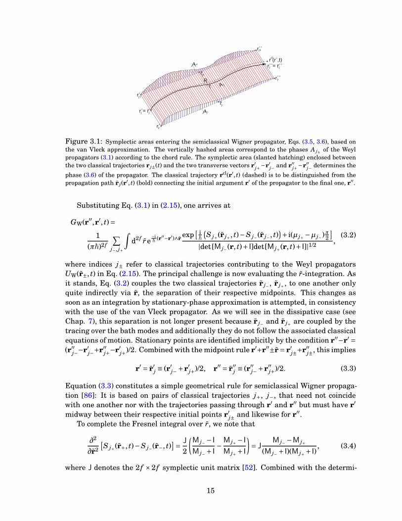
Figure 3.1: Symplectic areas entering the semiclassical Wigner propagator, Eqs. (3.5, 3.6), based onthe van Vleck approximation. The vertically hashed areas correspond to the phases A j± of the Weylpropagators (3.1) according to the chord rule. The symplectic area (slanted hatching) enclosed betweenthe two classical trajectories r j±(t) and the two transverse vectors r′j+−r′j− and r′′j+−r′′j− determines the

phase (3.6) of the propagator. The classical trajectory rcl(r′, t) (dashed) is to be distinguished from thepropagation path r j(r′, t) (bold) connecting the initial argument r′ of the propagator to the final one, r′′.

Substituting Eq. (3.1) in (2.15), one arrives at

GW(r′′,r′, t)=

1

(π~)2 f

∑

j−, j+

∫

d2 f re−i~

(r′′−r′)∧rexp

[ i~

(

S j+(r j+, t)−S j−(r j−, t))

+ i(µ j+ −µ j−)π2]

|det[M j−(r, t)+ I]det[M j+(r, t)+ I]|1/2,

(3.2)

where indices j± refer to classical trajectories contributing to the Weyl propagatorsUW(r±, t) in Eq. (2.15). The principal challenge is now evaluating the r-integration. Asit stands, Eq. (3.2) couples the two classical trajectories r j−, r j+, to one another onlyquite indirectly via r, the separation of their respective midpoints. This changes assoon as an integration by stationary-phase approximation is attempted, in consistencywith the use of the van Vleck propagator. As we will see in the dissipative case (seeChap. 7), this separation is not longer present because r j− and r j+ are coupled by thetracing over the bath modes and additionally they do not follow the associated classicalequations of motion. Stationary points are identified implicitly by the condition r′′−r′ =(r′′j−−r′j−+r′′j+−r′j+)/2. Combined with the midpoint rule r′+r′′±r= r′j±+r′′j±, this implies

r′ = r′j ≡ (r′j−+r′j+)/2, r′′ = r′′j ≡ (r′′j−+r′′j+)/2. (3.3)

Equation (3.3) constitutes a simple geometrical rule for semiclassical Wigner propaga-tion [86]: It is based on pairs of classical trajectories j+, j−, that need not coincidewith one another nor with the trajectories passing through r′ and r′′ but must have r′

midway between their respective initial points r′j± and likewise for r′′.To complete the Fresnel integral over r, we note that

∂2

∂r2

[

S j+(r+, t)−S j−(r−, t)]

= J

2

(

M j− − I

M j− + I−M j+ − I

M j+ + I

)

= JM j− −M j+

(M j− + I)(M j+ + I), (3.4)

where J denotes the 2 f ×2 f symplectic unit matrix [52]. Combined with the determi-

15

nantal prefactors inherited from the van Vleck propagator, this produces

GvVW (r′′,r′, t)=

4 f

h f

∑

j

2cos(

1~

SvVj (r′′,r′, t)−ν j

π4

)

|det(M j+ −M j−)|1/2, (3.5)

the semiclassical Wigner propagator in van Vleck approximation [1,2], ν j is the “indexof inertia” associated to the matrix M j+ −M j− and is given by the difference betweenthe numbers of positive and negative eigenvalues [99]. The phase of the propagator isdetermined by the action

SvVj (r′′,r′, t)= (r j+ − r j−)∧ (r′′− r′)+S j+ −S j−

=∫t

0ds

[

˙r j(s)∧r j(s)−H j+(r j+)+H j−(r j−)]

, (3.6)

with r j(s) ≡ (r j−(s)+ r j+(s))/2 and r j(s) ≡ r j+(s)− r j−(s). Besides the two Hamiltonianterms it includes the symplectic area enclosed between the two trajectory sections andthe vectors r′j+ −r′j− and r′′j+ −r′′j− (Fig. 3.1).

In the following we list a number of general features of Eqs. (3.5,3.6):

i. Equation (3.5) replaces the Liouville propagator,

GclW(r′′,r′, t)= δ

[

r′′−rcl(r′, t)]

, (3.7)

localized on the classical trajectory rcl(r′, t) initiated in r′, by a “quantum spot”, asmooth distribution peaked at the support of the classical propagator but spread-ing into the adjacent phase space off the classical trajectory and structured by anoscillatory pattern that results from the interference of the trajectories involved.

ii. The propagator (3.5) does involve determinantal prefactors. However, they donot result from any projection onto a subspace of phase space like q or p and aremanifestly invariant [52] under linear canonical (affine) transformations [100].

iii. It deviates from the Liouville propagator if and only if the potential is anhar-monic. For a purely harmonic potential, the two operations, propagation in timeand forming midpoints between trajectories, commute, so that all midpoint pathsr j(t)= [r j−(t)+r j+(t)]/2 coincide with each other and with the classical trajectoryrcl(r′, t). This singularity restores the classical delta function on rcl(r′, t), the in-terested reader may also want to consult Ref. [2] for further details.

iv. The only condition restricting the choice of trajectory pairs to be included in thecalculation of the propagator is the midpoint rule (3.3). It does, however, not con-stitute a double-sided boundary condition since every pair fulfilling Eq. (3.3) forthe initial points contributes a valid data point to the propagator. Therefore, thereis no root-search problem. In particular, the freedom in the choice of trajectorypairs can be exploited to optimize numerical implementations.

16

v. The propagator’s oscillatory pattern encodes and transmits information on quan-tum coherences. In particular, it allows us to propagate the “sub-Planckian os-cillations” [101] characterizing the Wigner function. In this sense, Eqs. (3.5, 3.6)solve the problem of the “dangerous cross terms” pointed out by Heller [102]. Thisissue is addressed in the next chapter.

vi. The principle of propagation by trajectory pairs is consistent with the proper-ties of a dynamical group. It translates the concatenation of propagators into apairwise continuation of trajectories, if the convolution integral in Eq. (2.16) isevaluated by stationary-phase approximation as well.

vii. Equations (3.5, 3.6) fail if the stationary points approach each other too closely.This is the case for short time and, for any time, near the central peak of thepropagator on the classical trajectory. Moreover, the problem arises systemati-cally in the limit of weak anharmonicity and in the classical limit. Therefore,these cases require an improved treatment by means of a uniform approximationto the r-integration in Eq. (3.2), see [2].

3.2 From Van Vleck Propagator to Semiclassical Wig-

ner Propagator

An alternative expression for the semiclassical propagator of the Wigner function canbe obtained if we replace the semiclassical expression of the unitary time-evolutionoperator derived by van Vleck propagator in (2.23),

GW(r′′, t;r′,0)=1

(2π~) f

∑

j, j′

∣

∣

∣

∣

∣

∂2R j

∂q′n∂q′′

m

∣

∣

∣

∣

∣

1/2 ∣

∣

∣

∣

∣

∂2R j′

∂q′n∂q′′

m

∣

∣

∣

∣

∣

1/2∫

df q′df q′′exp{

i

~(p′ · q′−p′′ · q′′)

}

exp{

i

~R j

(

q′′+ 1

2q′′, t;q′+ 1

2q′, t

)

− i

~R j′

(

q′′− 1

2q′′, t;q′− 1

2q′, t

)

+ (µ j −µ j′)π

2

}

.

To be consistent with the van Vleck approximation, integrations over q′ and q′′ mustbe performed at the level of stationary-phase approximation. In this case, it impliesthat

p′ = 1

2

(

p′j

(

q′)+p′j′(

q′))

, p′′ = 1

2

(

p′′j

(

q′′)+p′′j′(

q′′))

. (3.8)

On the other hand, since q′′ and q′ are the midpoints between the final and initialconditions of R j

(

q′′+ 12 q′′, t;q′+ 1

2 q′, t)

and R j(

q′′− 12 q′′, t;q′− 1

2 q′, t)

, respectively, wecan express them in terms of the coordinates q+ = (q+ q)/2 and q− = q− q, so we canshortly write

r′′ =1

2

(

r′′++r′′−)

, r′ =1

2

(

r′++r′−)

, (3.9)

which corresponds to the same midpoint rule derived in last section [see Eq. (3.3)].Before evaluating the action along these paths, we calculate the amplitude of eachcontribution, it can be expressed in terms of the difference of the stability matrices

17

associated to r+ and r−, (cf. Appendix A for a related calculation), i.e.

1

det(

M j+ −M j−

) =det

(

∂2R j+∂q′

j+∂q′′j+

)

det(

∂2R j−∂q′

j−∂q′′j−

)

det

∂2R j+∂q′

j+∂q′j+− ∂2R j−

∂q′j−∂q′

j−

∂2R j+∂q′

j+∂q′′j+− ∂2R j−

∂q′j−∂q′′

j−∂2R j+

∂q′′j+∂q′

j+− ∂2R j−

∂q′′j−∂q′

j−

∂2R j+∂q′′

j+∂q′′j+− ∂2R j−

∂q′′j−∂q′′

j−

. (3.10)

This relation certainly reduces the evaluation of amplitude of each contribution andprovides the same amplitude as the one derived using the previous approach. Wenote that the action p′ ·q′−p′′ ·q′′+R j

(

q′′+ 12Q′′, t;q′+ 1

2Q′, t)

−R j(

q′′− 12Q′′, t;q′− 1

2Q′, t)

can be expressed in terms of the energy along the trajectory HW(

r j ± 12 r j

)

and thesymplectic product between r∧ r as

∫t0 dt

[

r∧ r−H j+

(

r+ 12 r

)

+H j−

(

r− 12 r

)]

. Based onthis fact and from (3.10), we get finally

GW(r′′, t;r′,0)=4 f

h f

∑

j

2cos(

1~

SvVj (r′′,r′, t)−ν j

π4

)

∣

∣det(

M j+ −M j−

)∣

∣

1/2, (3.11)

with SvVj (r′′,r′, t) given by (3.6). So, we that propagation of the density matrix by two

van Vleck propagators is completely equivalent, as one could expect, to propagate theassociated Wigner function with (3.11). An alternative route towards the semiclassicalWigner propagator can be derive from the Marinov’s path integral approach describedpreviously in Sec. 2.3.2, this route is exploring in the next section.

3.3 From Phase-Space Path-Integrals to Semiclassi-

cal Wigner Propagator

In this section we evaluate the path-integral expression for the Wigner propagatorgiven in (2.28) making use of the stationary-phase approximation. In order to calculatethe extremal trajectories maximizing the action S[{r}, {r},t],

∂S

∂r= 0,

∂S

∂r= 0, (3.12)

we calculate the derivatives of S[{r}, {r},t] in the discrete-time version (2.25). Aftertaking the continuous limit and defining r± = r± r

2 , we get that the action is maximizedby the trajectories r± satisfying [1,6]

r± = J∇HW(r±), (3.13)

which means that r±, not only determine the propagation in phase space, but also aresolutions of the classical equation of motion. This picture changes dramatically by theintroduction of dissipation in Chapter 7. In this case, the path-integral expressions arereplaced by summation over these trajectories and weighted by the second derivatives

18

of the action along these trajectories. As in previous cases, this second-derivativesmatrix can be related to the difference of the stability matrices of r+ and r−,

det

∂2S[{r},{r},t]∂q2

∂2S[{r},{r},t]∂p2

∂2S[{r},{r},t]∂q2

∂2S[{r},{r},t]∂p2

= 1

4 fdet

∂q′′+

∂q′+− ∂q′′

−∂q′

−

∂q′′+

∂p′+− ∂q′′

−∂p′

−∂p′′

+∂q′

+− ∂p′′

−∂q′

−

∂p′′+

∂p′+− ∂p′′

−∂p′

−

= 1

4 fdet(M+−M−).

(3.14)Since the summation over trajectories contains terms j+ j− and j− j+ we can guaranteethat the propagator is real, taking into account last arguments, we can show that thepropagator takes the form

GW(r′′, t;r′,0)=4 f

h f

∑

j

2cos(

1~

SvVj (r′′,r′, t)−ν j

π4

)

∣

∣det(

M j+ −M j−

)∣

∣

1/2, (3.15)

with SvVj (r′′,r′, t) given by (3.6). From here we can see that these tree approaches leaves

exactly with the same expression for the semiclassical Wigner propagator (3.5), (3.11)or (3.15).

3.4 From Liouville-Propagator Eigenfunctions to Se-

miclassical Wigner Propagator

In section (2.3.2) we derived an expression for the Wigner propagator in terms of theeigenfunctions of the associated Hamiltonian (2.21),

GW(r′′, t;r′,0)= (2π~) f∑

n,mexp

(

−iEn −Em

~t)

ρW,nm(r′′)ρW,mn(r′),

where we called ρW,nm(r′′) the mixed Wigner functions. According to Brumer et al.’[103–107], the product of these Wigner functions, ρW,nm(r′′)ρW,mn(r′), can be under-stood as the eigenfunctions of the Liouville propagator. This remark allowed Brumeret al. to identify the classical analogues of the quantum eigenfunction of the Liouvillepropagator. However, in their analysis there was not any particular mention to thesemiclassical case. Based on Brumer et al.’ work, one can conclude that a derivationof the semiclassical Wigner propagator following this approach would imply differenttreatments for integrable [106] or chaotic [107] systems and would allow for a semiclas-sical description of finite size quantum systems [104]. For our proposes, expressions(3.5), (3.11) or (3.15) are enough and we leave this very interesting alternative for afuture work.

19

CHAPTER 4

Semiclassical Description of Quantum Coherences in

Phase Space

The major challenge for any attempt to directly propagate Wigner functions is theappropriate treatment of quantum coherences. As was pointed out by Heller [102], thenon-diagonal elements of the density matrix, which are usually encoded in the Wignerfunction through “sub-Planckian" oscillations [101], can give rise to a complete failureof semiclassical propagation of the Wigner function.

In this chapter, we make use of the semiclassical approximation (3.5, 3.6) to providea semiclassical description of quantum systems in the presence of marked quantumeffects, e.g., coherent tunneling and propagating Schrödinger cat-states.

4.1 Semiclassical Propagation of Schrödinger’s Cat-

States

Schrödinger cats are a paradigm of quantum coherence and embody the basics of en-tanglement in a simple setting. They allow us to test the performance of propagationmethods in this particular respect in an objective manner, as the separation of thesuperposed alternatives and thus the wavelength of the corresponding interferencepattern can be precisely controlled.

Since we here consider the propagation of Schrödinger cat-states prepared as the co-herent superposition of two Gaussian states, we consider illustrative to translate first asingle Gaussian state into the phase-space language. In the context of the Wigner rep-resentation, Gaussians gain special relevance as they constitute the only admissibleWigner functions that are positive definite and therefore can be interpreted in terms ofprobabilities [108]. They have achieved a fundamental rôle for semiclassical propaga-tion as they provide a natural smoothing which allows to reduce the time-evolution ofan entire phase-space region to the propagation along a single classical trajectory.

20

Define Gaussians in phase space [109] by

W(r)=p

detA

(2π~) fexp

[

−(r−r0) ·A(r−r0)

2~

]

. (4.1)

The 2 f × 2 f -covariance matrix A controls size, shape, and orientation of the Gaus-sian centered in r0 = (p0,q0). The more specific class of minimum-uncertainty Gaus-sians, equivalent to Wigner representations of coherent states [110], is characterizedby detA= 1. In what follows, in two dimensions r= (p, q), we choose A= diag(1/γ,γ), sothat

ρW(r)= 1

π~exp

[

− (p− p0)2 +γ2(q− q0)2

γ~

]

. (4.2)

In this way, we have that the Schrödringer cat-state is defined by

ρW,cat(r)= ρW,−(r)+ρW,+(r)+ρW,×(r), (4.3)

where ρW,±(r)= exp{−[p2±+γ2q2

±]/γ~}/(π~), r± = r− [r0 ± (0, d)], while

ρW,×(r)=exp{−[(p− p0)2 +γ2(q− q0)2]/γ~}cos[2(p− p0)d/~] (4.4)

encodes the quantum coherence in terms of “sub-Planckian” oscillations of wavelength~/d in p [101].

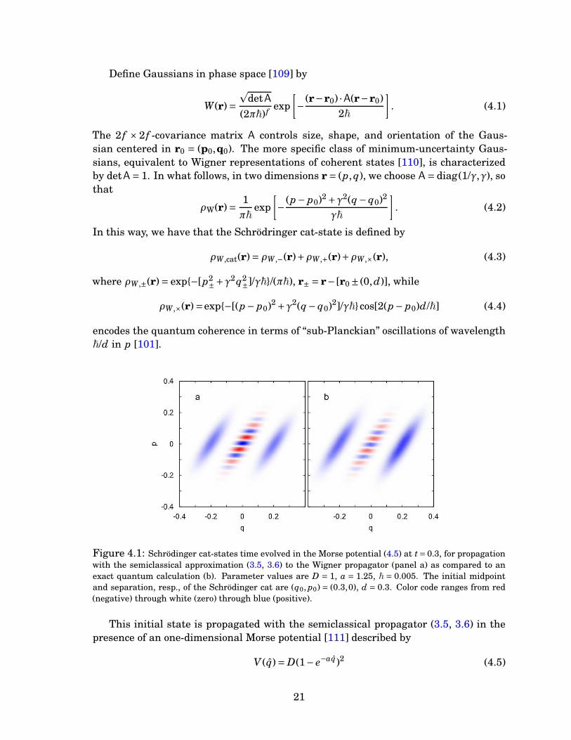
Figure 4.1: Schrödinger cat-states time evolved in the Morse potential (4.5) at t= 0.3, for propagationwith the semiclassical approximation (3.5, 3.6) to the Wigner propagator (panel a) as compared to anexact quantum calculation (b). Parameter values are D = 1, a = 1.25, ~ = 0.005. The initial midpointand separation, resp., of the Schrödinger cat are (q0, p0) = (0.3,0), d = 0.3. Color code ranges from red(negative) through white (zero) through blue (positive).

This initial state is propagated with the semiclassical propagator (3.5, 3.6) in thepresence of an one-dimensional Morse potential [111] described by

V (q)= D(1− e−aq)2 (4.5)

21

and determined by the depth D and inverse width a of the potential well. We choose theMorse oscillator because it is prototypical for strongly anharmonic molecular potentialsand correspondingly complex dynamics, widely used as a benchmark for numericalmethods in this realm [112–116].

The result is compared in Fig. 4.1 to the exact quantum calculation. Despite minordeviations in the shape of the Gaussian envelopes, the interference pattern is perfectlyreproduced. This is not surprising in view of the trajectory-pair construction underly-ing our semiclassical approximation.

In fact, it is instructive to see why propagating along the two classical trajectoriesof the respective centroids of the two “classical” Gaussians ρW,±(r) already reproducesessentially the sub-Planckian oscillations. The propagator starting from the centroidr0 of the oscillatory pattern then comprises two terms, GW(r′′,r0, t) = GW0(r′′,r0, t)+GW×(r′′,r0, t). According to Eqs. (3.5, 3.6), the first one, propagating along the clas-sical trajectory rcl(r0, t) that passes through r0, bears no oscillating phase factor andtherefore practically cancels upon convolution with the strongly oscillatory ρW,×(r′).The second one, by contrast, is the contribution of the two centroid orbits rcl(r±, t)forming a pair of non-identical trajectories. It travels along the midpoint path r×(t) =(rcl(r−, t)+rcl(r+, t))/2 and carries a phase factor ∼ cos[(2/~)(r+−r−)∧r′] = cos[2dp′/~]which couples resonantly to the oscillations in ρW,×(r′).

4.2 Semiclassical Description of Tunneling

Tunneling is to be regarded a quantum coherence effect “of infinite order in ~” [55]. Onetherefore does not expect a particularly good performance of semiclassical propagationmethods in the description of tunneling, despite various efforts that have been made toimprove them in this respect. Above all, the complexification of phase space provides asystematic approach to include tunneling in a semiclassical framework [117–119].

In the present work we restrict ourselves to real phase-space, in order not to loosethe valuable close relationship between Wigner and classical dynamics. Even so, we ex-pect that in this framework tunneling can be reproduced to a certain degree [120,121].To be sure, Wigner dynamics (in real phase space) is exact for harmonic potentials. Thisincludes parabolic barriers and hence a specific case of tunneling. This remarkablefact has been indicated and explained by Balazs and Voros in Ref. [120]: As the Wignerpropagator invariably follows classical trajectories, the explanation rather refers tothe initial condition in Wigner representation which, owing to quantum uncertainty,spills over the separatrix even if it is concentrated at negative energies, and thus istransported in part along classical trajectories to the other side of the barrier.

This is to be considered as a fortunate exception, though, and other, more typicalcases involving genuine quantum effects, like in particular coherent tunneling betweenbound states, are not so readily accessible to semiclassical Wigner dynamics. Quantumtunneling in the Wigner representation, specifically for localized scattering potentials,has been studied at depth in [91,122], however without indicating a promising perspec-tive for semiclassical approximations. We are in a slightly more favourite situation asthe concept of propagation along trajectory pairs provides a viable option how to re-

22

r (t)cl+

r (t)cl

-

r(t)-

q

p

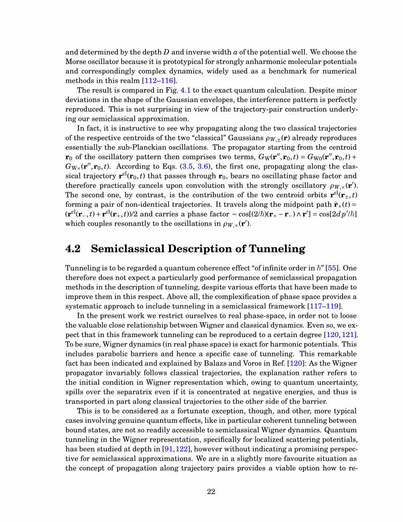
Figure 4.2: Semiclassical description of coherent tunneling in terms of trajectory pairs, in the frame-

work of the van Vleck based Wigner propagator (3.5, 3.6). A wavepacket initially prepared near the right

minimum of a double-well potential (blue patch) can be transported along a non-classical midpoint path

r(t) (dashed red line) into the opposite well if the two classical orbits rcl±(t) (full red lines) underlying

this path through r(t) = (rcl−(t)+rcl

+(t))/2 are sufficiently separated initially, e.g., rcl+ on the same side but

above the barrier, rcl− within the opposite well. Other contours of the potential and the separatrix are

indicated by black curves.

produce tunneling by means of a semiclassical Wigner propagator: As illustrated in(Fig. 4.2), it is trajectory pairs with sufficiently separated initial points, probing re-gions in phase space mutually inaccessible in terms of the classical dynamics, whichlead to transport in phase space along classically forbidden paths.

0

0.2

0.4

0.6

0.8

1

0 2 4 6 8 10 12

|C(t

)|2

t

a

q

p

0.8

0.85

0.9

0.95

1

0 0.5 1 1.5 2 2.5 3 3.5 4

t

b

q

p

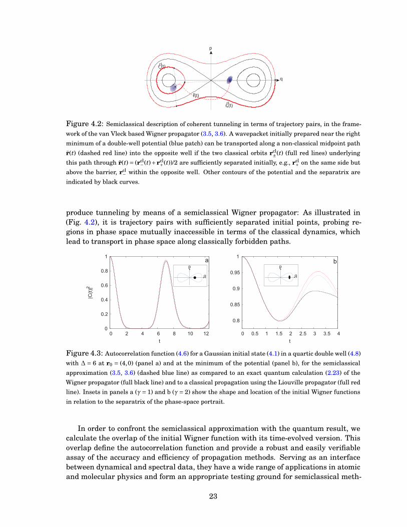
Figure 4.3: Autocorrelation function (4.6) for a Gaussian initial state (4.1) in a quartic double well (4.8)

with ∆ = 6 at r0 = (4,0) (panel a) and at the minimum of the potential (panel b), for the semiclassical

approximation (3.5, 3.6) (dashed blue line) as compared to an exact quantum calculation (2.23) of the

Wigner propagator (full black line) and to a classical propagation using the Liouville propagator (full red

line). Insets in panels a (γ= 1) and b (γ= 2) show the shape and location of the initial Wigner functions

in relation to the separatrix of the phase-space portrait.

In order to confront the semiclassical approximation with the quantum result, wecalculate the overlap of the initial Wigner function with its time-evolved version. Thisoverlap define the autocorrelation function and provide a robust and easily verifiableassay of the accuracy and efficiency of propagation methods. Serving as an interfacebetween dynamical and spectral data, they have a wide range of applications in atomicand molecular physics and form an appropriate testing ground for semiclassical meth-

23

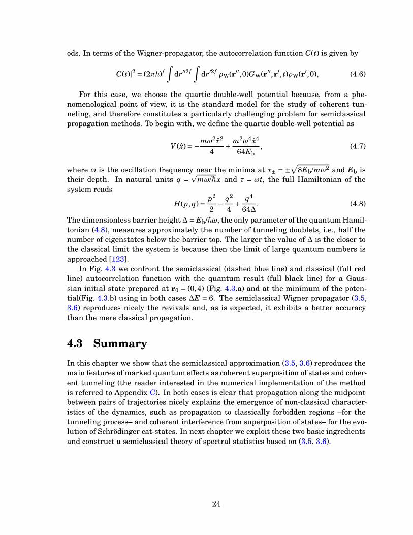
ods. In terms of the Wigner-propagator, the autocorrelation function C(t) is given by

|C(t)|2 = (2π~) f∫

dr′′2 f∫

dr′2 f ρW(r′′,0)GW(r′′,r′, t)ρW(r′,0), (4.6)

For this case, we choose the quartic double-well potential because, from a phe-nomenological point of view, it is the standard model for the study of coherent tun-neling, and therefore constitutes a particularly challenging problem for semiclassicalpropagation methods. To begin with, we define the quartic double-well potential as

V (x)=−mω2 x2

4+

m2ω4 x4

64Eb, (4.7)

where ω is the oscillation frequency near the minima at x± = ±√

8Eb/mω2 and Eb istheir depth. In natural units q =

pmω/~x and τ = ωt, the full Hamiltonian of the

system reads

H(p, q)= p2

2− q2

4+ q4

64∆. (4.8)

The dimensionless barrier height ∆= Eb/~ω, the only parameter of the quantum Hamil-tonian (4.8), measures approximately the number of tunneling doublets, i.e., half thenumber of eigenstates below the barrier top. The larger the value of ∆ is the closer tothe classical limit the system is because then the limit of large quantum numbers isapproached [123].

In Fig. 4.3 we confront the semiclassical (dashed blue line) and classical (full redline) autocorrelation function with the quantum result (full black line) for a Gaus-sian initial state prepared at r0 = (0,4) (Fig. 4.3.a) and at the minimum of the poten-tial(Fig. 4.3.b) using in both cases ∆E = 6. The semiclassical Wigner propagator (3.5,3.6) reproduces nicely the revivals and, as is expected, it exhibits a better accuracythan the mere classical propagation.

4.3 Summary

In this chapter we show that the semiclassical approximation (3.5, 3.6) reproduces themain features of marked quantum effects as coherent superposition of states and coher-ent tunneling (the reader interested in the numerical implementation of the methodis referred to Appendix C). In both cases is clear that propagation along the midpointbetween pairs of trajectories nicely explains the emergence of non-classical character-istics of the dynamics, such as propagation to classically forbidden regions –for thetunneling process– and coherent interference from superposition of states– for the evo-lution of Schrödinger cat-states. In next chapter we exploit these two basic ingredientsand construct a semiclassical theory of spectral statistics based on (3.5, 3.6).

24

CHAPTER 5

Quantum Coherences and Semiclassical Spectral

Statistics

One of the most fundamental questions of quantum chaos is why, in the semiclassi-cal limit, almost any classically hyperbolic system exhibits energy levels, eigenstates,transition amplitudes or transport properties which in a statistical sense are universaland depend only on the presence or absence of certain kind of symmetries [124]. Thisfact was conjectured by Bohigas, Giannoni and Schmit [125] and is by now well es-tablished by overwhelming numerical grounds and experimental evidence from atomicand molecular spectroscopy of classical micro-wave billiards in the limit of large quan-tum numbers [126,127].

With the aim of studying that universal character, we need to consider statisticalproperties like, e.g., fluctuations in the distribution of energy levels, which are givenby correlations between the eigenstates of the quantum system. These correlations aredescribed by the two-point correlation function or cluster function Y2(E) [128], whichis bilinear in the density of states d(E). In the semiclassical regime, d(E) is given bythe celebrated Gutzwiller’s trace formula [25]

d(E)≈ ⟨d⟩+ 1

π~Re

∑

jA je

iS j (E)/~, (5.1)

where ⟨d⟩ is the mean density of states and j labels the periodic orbits of the chaoticsystem. The contribution from each orbit is characterized by its classical action S j

and is weighted by the amplitude A j, which depends on the period T j, on the stabilitymatrix and on the number of conjugated points of the orbit. This expression providesa direct relation between the spectral quantities related to the quantum HamiltonianH and the dynamical quantities generated by the classical Hamiltonian H.

In time-domain, those correlation between states are described by the Fourier trans-form of Y2(E), i.e., by the form factor K (τ). In terms of the Gutzwiller’s trace formula,

25

the semiclassical form factor reads (cf. [124]),

K (τ)= 1

2π~⟨d⟩∑

j j′

⟨

A j A∗j′e

i(S j−S j′ )/~δ

(

T −T j −T j′

2

)⟩

E, (5.2)

where τ= T/(2π~ ⟨d⟩) and ⟨·⟩E denotes an average over an energy window [124,128].Since the number of periodic orbits increase exponentially with the period [124,129]

then the double sum contains a huge number of pair terms. Most of the pair consistof pairs with non-correlated actions and their contributions cancel each other whensummed over, in this way, it is expected that non-vanishing contributions come fromcorrelated pairs. The strongest correlation occur between trajectories having identicalactions, so would be natural to restrict the sum over identical trajectories or relatedby time-reversal, i.e., would be natural to evaluate the double sum in the diagonalapproximation. However, in order to prove the universality conjectured by Bohigas etal. [125], non-diagonal terms are requisite. This fact generated that in last years allattention was focused on going beyond the diagonal approximation and only recentlya successful attempt to deal with the whole sum was done [130], notwithstanding thequantum-classical correspondence of the terms contributing, even in the diagonal ap-proximation, to the double sum is not completely clear.

In order to resolve the classical structures contributing to (5.2), a promissory re-lation between the spectral form factor K (τ) and the classical probability to returnPcl

ret(t) has been made in the context of the spectral analysis of systems with dynamicallocalization [128,131,132]. For chaotic systems it reads

K (τ)≈ (2/β)τPclret(tHτ), (5.3)

where β= 1 (2) in the presence (absence) of time-reversal invariance. Based on the di-agonal approximation, the expression is valid for times short compared to the Heisen-berg time tH = h⟨d⟩. A similar relation but without the prefactor τ holds for integrablesystems [128] and for chaotic systems with dissipation [75].

In next sections we show that the spectral form factor can be defined in terms of theWigner propagator and it will allow us to introduce the semiclassical approximation(3.5, 3.6) in a different context. We start defining the classical and quantum return-probabilities.

5.1 Classical and Quantum Return-Probabilities

In quantum mechanics, a probability to return is generally defined like an autocor-relation function: Introduce a return amplitude aret(t) =

∫

df q0⟨q(t)|q0⟩ with |q(t)⟩ =U(t)|q0⟩, U(t) the time-evolution operator, and square,

Pqmret (t)= |aret(t)|2 = |trU(t)|2. (5.4)

By contrast, a classical return probability in phase space is constructed as follows:Prepare a localized initial distribution ρr0(r,0) = δ∆(r− r0), δ∆(r) a strongly peaked

26

function of width ∆. Propagate it over a time t and overlap it with the initial distribu-tion. The resulting pcl

ret(r0, t) =∫

d2 f rρr0(r, t)ρr0(r,0) can be interpreted as a probabil-ity density to return. Here, the time-evolved distribution is obtained from the Liouvillepropagator Gcl(r′′, t;r′,0) as

ρr0(r′′, t)=∫

d2 f r′Gcl(r′′, t;r′,0)ρr0(r′,0). (5.5)

Tracing over phase space yields the return probability Pclret(t) =

∫

d2 f r0 pclret(r0, t). Re-

placing the initial distribution by δ(r−r0), we have

Pclret(t)=

∫

d2 f r0 Gcl(r0, t;r0,0). (5.6)

To avoid divergences in particular at t = 0, the phase-space integration has to be re-stricted to a finite range ∆E in energy, if it is conserved, by introducing some normal-ized energy distribution ρ(E) 1.

In quantum mechanics, the Wigner function allows for a similar construction. Byanalogy, we thus arrive at a quantum-mechanical quasi-probability density to returnin phase space [133], pqm

ret (r0, t)= GW(r0, t;r0,0), and a return probability

Pqmret (t)=

∫

d2 f r0 GW(r0, t;r0,0). (5.7)

The integration across the energy shell produces a factor DH = ∆E/⟨d⟩, the effectivedimension of the Hilbert space H . Equations (5.7) and (5.4) are equivalent, as be-comes clear if we express the propagator of the Wigner function in terms of the Weylpropagator (2.15). Substituting in Eq. (5.7)

Pqmret (t)=

∫

d2 f r∫

d2 f r′U∗W(r−r′/2; t,0)UW(r+r′/2; t,0)

=∫

d2 f r1U∗W(r1; t,0)

∫

d2 f r2UW(r2; t,0)

=∣

∣

∣

∣

∫

d2 f rUW(r; t,0)

∣

∣

∣

∣

2

=∣

∣trU(t,0)∣

∣

2. (5.8)

This relation expresses the form factor as a trace not as a squared trace, it implies thatinterference terms contributing to the form factor can be resolved.

1Upon letting ∆ → 0, care must be taken. In order that the return probability remain finite, somedynamical spreading of the distribution is required. Along certain phase-space directions, this doesnot occur, for example orthogonal to the energy shell in a conservative system or orthogonal to theinvariant torus in an integrable one. Restricting ourselves to the remaining directions r∥, we may thusreplace the smooth ρr0 (r,0) by a delta function, so that, taking a conservative chaotic system as anexample, pcl

ret(r0, t) =∫

d2 f −1r∥G(r0, t;r′ ,0)δ(r′ −r0) = Gcl(r0, t;r0 ,0), and tracing over the energy shell,Pcl

ret(t) =∫

shell dEρ(E)∫

d2 f −1r∥ Gcl(E,r∥, t;E,r∥ ,0), with some normalized energy distribution ρ(E). Inthe context of spectral analysis, it would define a narrow energy window ∆E as for a microcanonicalensemble [52].

27

5.2 Form Factor and Diagonal Propagator

Expression (5.8) allows us to make contact with spectral quantities if we recognize that

K (t/tH)= 1

DH

∣

∣trU(τtH,0)∣

∣

2, (5.9)

for t & tH/DH , where tH = h⟨d⟩. The factor D−1H

normalizes limτ→∞ K (τ) = 1. By com-parison with Eqs. (5.4) and (5.7),

Pqmret (t)=

∫

d2 f rGW(r, t;r,0)= DH K (t/tH). (5.10)

This remarkable relation expresses the form factor as the trace over a quantity witha close classical analogue, not as a squared trace. It is an exact identity and does notinvolve any semiclassical approximation.

Contrast Eq. (5.10) with (5.3). Both relate K (τ) with a return probability, but thereis a clear discrepancy, manifest in the factor τ that appears only in (5.3). This may notbe surprising given that the two relations refer to return probabilities on the quantumand the classical level, respectively. However, if we take into account also Eqs. (5.6)and (5.7),

Pqmret (t)=

∫

d2 f rGW(r, t;r,0)= DH K (t/tH)~→0= 2

βτPcl(t/tH)= 2

βτ

∫

d2 f rGcl(r, t/tH;r,0),

(5.11)we face a dilemma: There is ample evidence [1, 57, 134] that the Wigner propagatorgenerally converges in the classical limit to the Liouville propagator,

lim~→0

GW(r′′, t;r′,0)=Gcl(r′′, t;r′,0). (5.12)

For up to quadratic Hamiltonians, is even identical to it. Were Eq. (5.12) correct alsofor r′ = r′′—and on the diagonal the Wigner propagator should behave more classicallythan elsewhere—then lim~→0 Pqm

ret (t)= Pclret(t) should hold as well!

The derivation of Eq. (5.3) [128, 131, 132] suggests that the factor τ arises as a de-generacy factor due to the coherent superposition of contributions from different pointsalong a given periodic orbit, each of which can be interpreted as a periodic point of itsown, τ measuring the magnitude of this set in phase space. We therefore suspect thatEq. (5.12) might fail in the presence of constructive quantum interference. This canbe substantiated taking into account semiclassical approximations for GW(r′′, t;r′,0)based on pairs of classical trajectories rcl

−(t), rcl+(t) [1, 57]. Specifically for the diago-

nal propagator, this requires that both rcl−(t) and rcl

+(t) be periodic orbits. The set ofmidpoints r(t) = (rcl

−(t)+rcl+(t))/2 then forms a closed curve in phase space as well and

contributes to the diagonal propagator hence the form factor, but need not consist ofperiodic points proper.

It is tempting to interpret also the prefactor 2/β in Eq. (5.3) as a degeneracy fac-tor and to look for phase-space manifolds that in time-reversal invariant systems con-

28

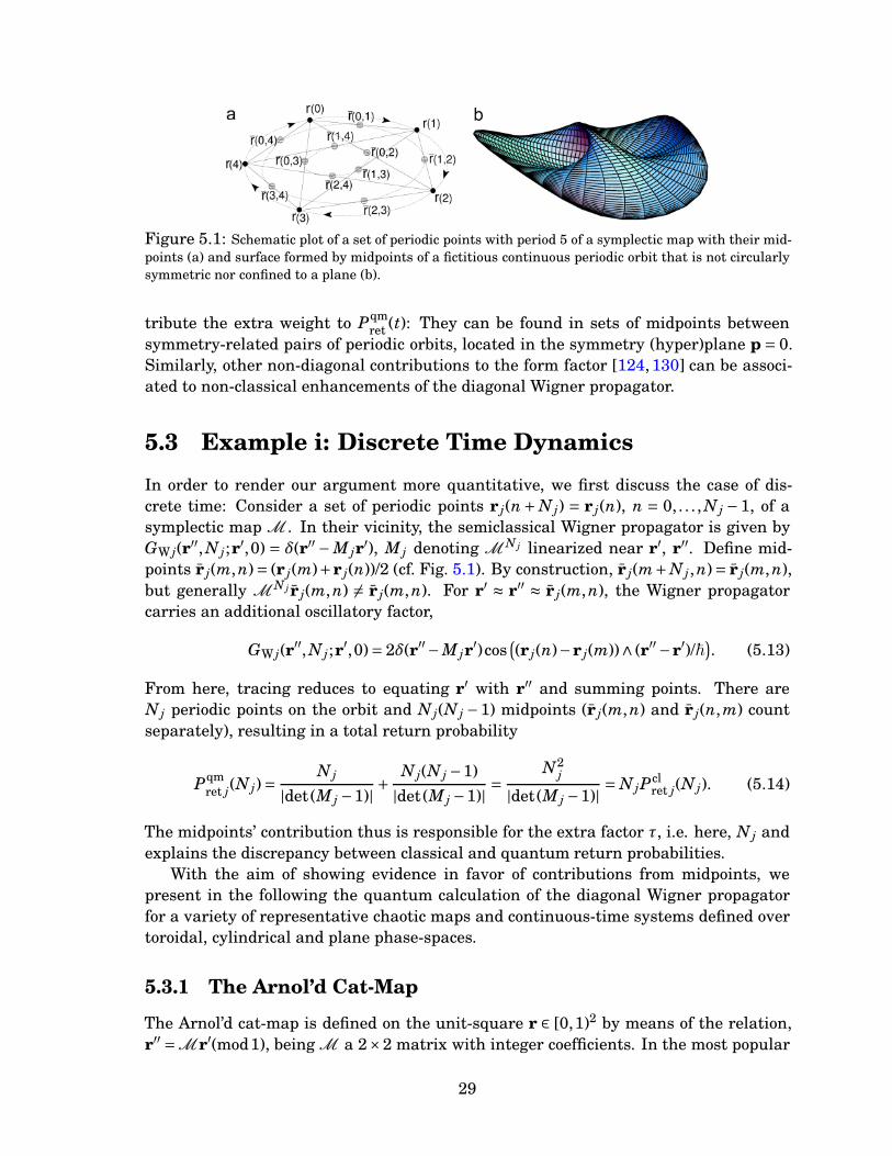
Figure 5.1: Schematic plot of a set of periodic points with period 5 of a symplectic map with their mid-points (a) and surface formed by midpoints of a fictitious continuous periodic orbit that is not circularlysymmetric nor confined to a plane (b).

tribute the extra weight to Pqmret (t): They can be found in sets of midpoints between

symmetry-related pairs of periodic orbits, located in the symmetry (hyper)plane p = 0.Similarly, other non-diagonal contributions to the form factor [124, 130] can be associ-ated to non-classical enhancements of the diagonal Wigner propagator.

5.3 Example i: Discrete Time Dynamics

In order to render our argument more quantitative, we first discuss the case of dis-crete time: Consider a set of periodic points r j(n+ N j) = r j(n), n = 0, . . . , N j −1, of asymplectic map M . In their vicinity, the semiclassical Wigner propagator is given byGW j(r′′, N j;r′,0) = δ(r′′− M jr

′), M j denoting MN j linearized near r′, r′′. Define mid-

points r j(m, n)= (r j(m)+r j(n))/2 (cf. Fig. 5.1). By construction, r j(m+N j, n)= r j(m, n),but generally M

N j r j(m, n) 6= r j(m, n). For r′ ≈ r′′ ≈ r j(m, n), the Wigner propagatorcarries an additional oscillatory factor,

GW j(r′′, N j;r

′,0)= 2δ(r′′−M jr′)cos

(

(r j(n)−r j(m))∧ (r′′−r′)/~)

. (5.13)

From here, tracing reduces to equating r′ with r′′ and summing points. There areN j periodic points on the orbit and N j(N j −1) midpoints (r j(m, n) and r j(n, m) countseparately), resulting in a total return probability

Pqmret j(N j)=

N j

|det(M j −1)|+

N j(N j −1)

|det(M j −1)|=

N2j

|det(M j −1)|= N jP

clret j(N j). (5.14)

The midpoints’ contribution thus is responsible for the extra factor τ, i.e. here, N j andexplains the discrepancy between classical and quantum return probabilities.

With the aim of showing evidence in favor of contributions from midpoints, wepresent in the following the quantum calculation of the diagonal Wigner propagatorfor a variety of representative chaotic maps and continuous-time systems defined overtoroidal, cylindrical and plane phase-spaces.

5.3.1 The Arnol’d Cat-Map

The Arnol’d cat-map is defined on the unit-square r ∈ [0,1)2 by means of the relation,r′′ =Mr′(mod1), being M a 2×2 matrix with integer coefficients. In the most popular

29

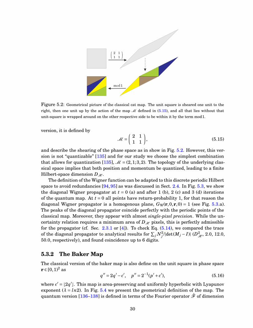
Figure 5.2: Geometrical picture of the classical cat map. The unit square is sheared one unit to the

right, then one unit up by the action of the map M defined in (5.15), and all that lies without that

unit-square is wrapped around on the other respective side to be within it by the term mod1.

version, it is defined by

M =(

2 11 1

)

, (5.15)

and describe the shearing of the phase space as in show in Fig. 5.2. However, this ver-sion is not “quantizable” [135] and for our study we choose the simplest combinationthat allows for quantization [135], M = (2,1;3,2). The topology of the underlying clas-sical space implies that both position and momentum be quantized, leading to a finiteHilbert-space dimension DH .

The definition of the Wigner function can be adapted to this discrete periodic Hilbertspace to avoid redundancies [94,95] as was discussed in Sect. 2.4. In Fig. 5.3, we showthe diagonal Wigner propagator at t = 0 (a) and after 1 (b), 2 (c) and 3 (d) iterationsof the quantum map. At t = 0 all points have return-probability 1, for that reason thediagonal Wigner propagator is a homogenous plane, GW(r,0,r,0) = 1 (see Fig. 5.3.a).The peaks of the diagonal propagator coincide perfectly with the periodic points of theclassical map. Moreover, they appear with almost single-pixel precision. While the un-certainty relation requires a minimum area of DH pixels, this is perfectly admissiblefor the propagator (cf. Sec. 2.3.1 or [4]). To check Eq. (5.14), we compared the traceof the diagonal propagator to analytical results for

∑

j N2j /|det(M j − I)| (D2

H, 2.0, 12.0,

50.0, respectively), and found coincidence up to 6 digits.

5.3.2 The Baker Map

The classical version of the baker map is also define on the unit square in phase spacer ∈ [0,1)2 as

q′′ = 2q′−ε′, p′′ = 2−1(p′+ε′), (5.16)

where ε′ = b2q′c. This map is area-preserving and uniformly hyperbolic with Lyapunovexponent (λ = ln2). In Fig. 5.4 we present the geometrical definition of the map. Thequantum version [136–138] is defined in terms of the Fourier operator F of dimension

30

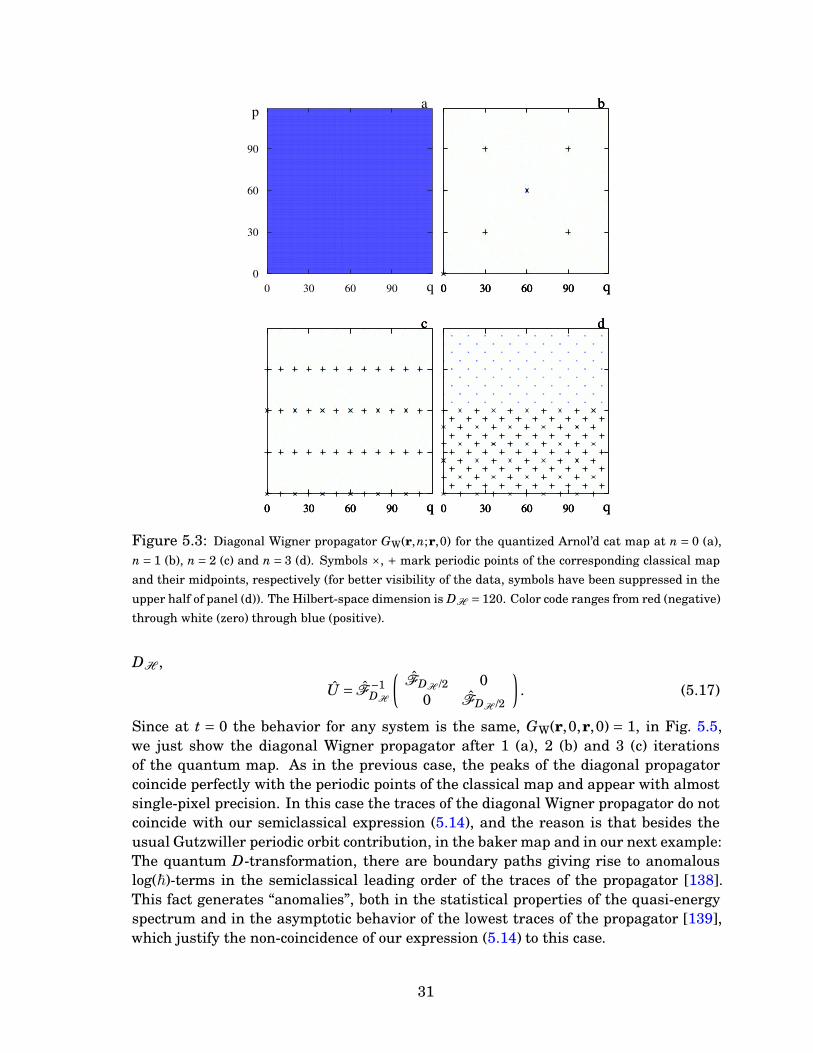
p

q

a

9060300

90

60

30

0

q

b

9060300

q

b

9060300

q

b

9060300

q

c

9060300

q

c

9060300

q

c

9060300

q

d

9060300

q

d

9060300

q

d

9060300

Figure 5.3: Diagonal Wigner propagator GW(r,n;r,0) for the quantized Arnol’d cat map at n = 0 (a),

n = 1 (b), n = 2 (c) and n = 3 (d). Symbols ×, + mark periodic points of the corresponding classical map

and their midpoints, respectively (for better visibility of the data, symbols have been suppressed in the

upper half of panel (d)). The Hilbert-space dimension is DH = 120. Color code ranges from red (negative)

through white (zero) through blue (positive).

DH ,

U = F−1DH

(

FDH /2 00 FDH /2

)

. (5.17)

Since at t = 0 the behavior for any system is the same, GW(r,0,r,0) = 1, in Fig. 5.5,we just show the diagonal Wigner propagator after 1 (a), 2 (b) and 3 (c) iterationsof the quantum map. As in the previous case, the peaks of the diagonal propagatorcoincide perfectly with the periodic points of the classical map and appear with almostsingle-pixel precision. In this case the traces of the diagonal Wigner propagator do notcoincide with our semiclassical expression (5.14), and the reason is that besides theusual Gutzwiller periodic orbit contribution, in the baker map and in our next example:The quantum D-transformation, there are boundary paths giving rise to anomalouslog(~)-terms in the semiclassical leading order of the traces of the propagator [138].This fact generates “anomalies”, both in the statistical properties of the quasi-energyspectrum and in the asymptotic behavior of the lowest traces of the propagator [139],which justify the non-coincidence of our expression (5.14) to this case.

31

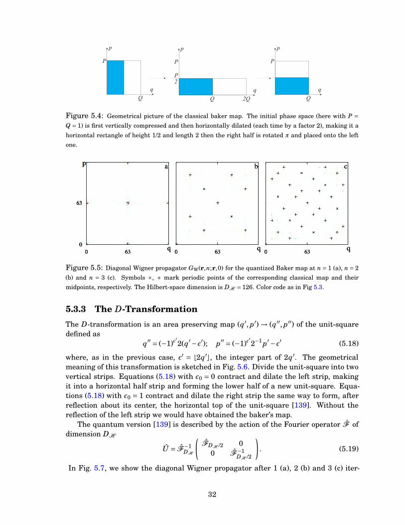
P

Q

p

q

P

Q

p

q

2Q

P2

P

Q

p

q

Figure 5.4: Geometrical picture of the classical baker map. The initial phase space (here with P =Q = 1) is first vertically compressed and then horizontally dilated (each time by a factor 2), making it a

horizontal rectangle of height 1/2 and length 2 then the right half is rotated π and placed onto the left

one.

p

q

a

630

63

0

p

q

a

630

63

0

p

q

a

630

63

0q

b

630q

b

630q

b

630q

c

630q

c

630q

c

630

Figure 5.5: Diagonal Wigner propagator GW(r,n;r,0) for the quantized Baker map at n = 1 (a), n = 2

(b) and n = 3 (c). Symbols ×, + mark periodic points of the corresponding classical map and their

midpoints, respectively. The Hilbert-space dimension is DH = 126. Color code as in Fig 5.3.

5.3.3 The D-Transformation

The D-transformation is an area preserving map (q′, p′) → (q′′, p′′) of the unit-squaredefined as

q′′ = (−1)ε′2(q′−ε′); p′′ = (−1)ε

′2−1 p′−ε′ (5.18)

where, as in the previous case, ε′ = b2q′c, the integer part of 2q′. The geometricalmeaning of this transformation is sketched in Fig. 5.6. Divide the unit-square into twovertical strips. Equations (5.18) with ε0 = 0 contract and dilate the left strip, makingit into a horizontal half strip and forming the lower half of a new unit-square. Equa-tions (5.18) with ε0 = 1 contract and dilate the right strip the same way to form, afterreflection about its center, the horizontal top of the unit-square [139]. Without thereflection of the left strip we would have obtained the baker’s map.

The quantum version [139] is described by the action of the Fourier operator F ofdimension DH

U = F−1DH

(

FDH /2 00 F

−1DH /2

)

. (5.19)

In Fig. 5.7, we show the diagonal Wigner propagator after 1 (a), 2 (b) and 3 (c) iter-

32

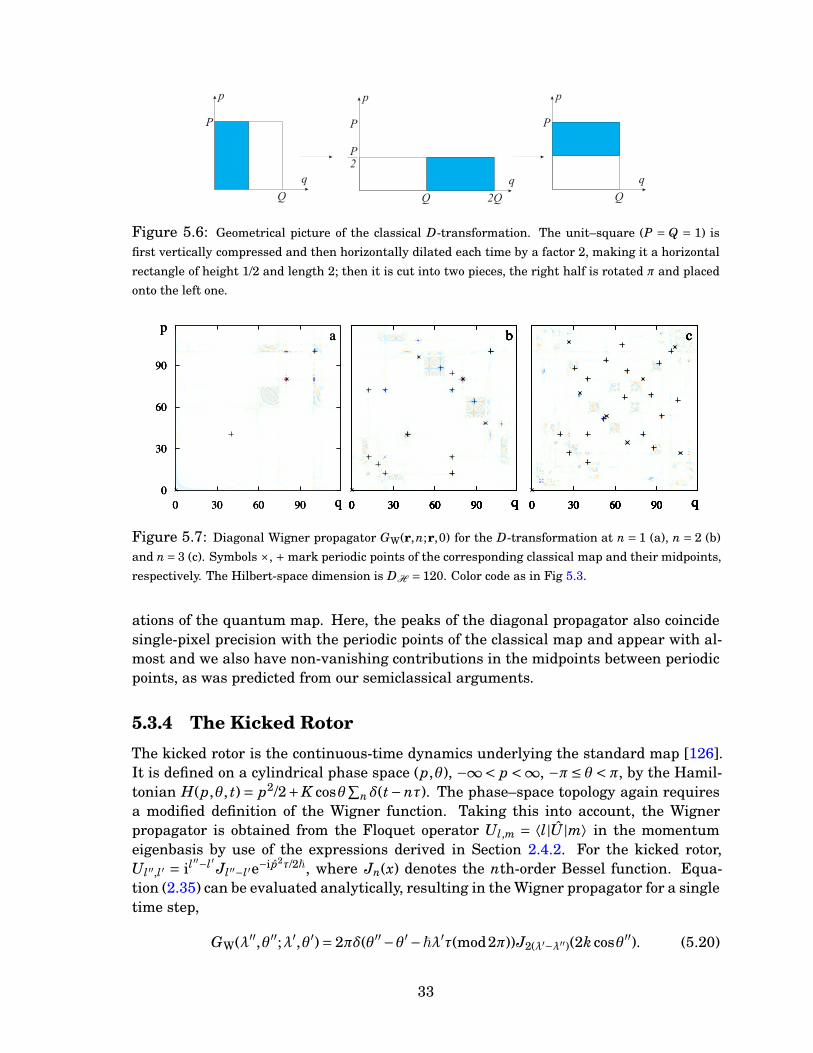
P

Q

p

q

P

Q

p

q

2Q

P2

P

Q

p

q

Figure 5.6: Geometrical picture of the classical D-transformation. The unit–square (P = Q = 1) is

first vertically compressed and then horizontally dilated each time by a factor 2, making it a horizontal

rectangle of height 1/2 and length 2; then it is cut into two pieces, the right half is rotated π and placed

onto the left one.

p

q

a

9060300

90

60

30

0

p

q

a

9060300

90

60

30

0

p

q

a

9060300

90

60

30

0

q

b

9060300 q

b

9060300 q

b

9060300 q

b

9060300 q

b

9060300 q

b

9060300 q

b

9060300 q

c

9060300 q

c

9060300 q

c

9060300 q

c

9060300 q

c

9060300 q

c

9060300 q

c

9060300

Figure 5.7: Diagonal Wigner propagator GW(r,n;r,0) for the D-transformation at n = 1 (a), n = 2 (b)

and n= 3 (c). Symbols ×, + mark periodic points of the corresponding classical map and their midpoints,

respectively. The Hilbert-space dimension is DH = 120. Color code as in Fig 5.3.

ations of the quantum map. Here, the peaks of the diagonal propagator also coincidesingle-pixel precision with the periodic points of the classical map and appear with al-most and we also have non-vanishing contributions in the midpoints between periodicpoints, as was predicted from our semiclassical arguments.

5.3.4 The Kicked Rotor

The kicked rotor is the continuous-time dynamics underlying the standard map [126].It is defined on a cylindrical phase space (p,θ), −∞< p <∞, −π≤ θ < π, by the Hamil-tonian H(p,θ, t) = p2/2+K cosθ

∑

nδ(t−nτ). The phase–space topology again requiresa modified definition of the Wigner function. Taking this into account, the Wignerpropagator is obtained from the Floquet operator Ul,m = ⟨l|U |m⟩ in the momentumeigenbasis by use of the expressions derived in Section 2.4.2. For the kicked rotor,Ul′′,l′ = il′′−l′ Jl′′−l′e−i p2τ/2~, where Jn(x) denotes the nth-order Bessel function. Equa-tion (2.35) can be evaluated analytically, resulting in the Wigner propagator for a singletime step,

GW(λ′′,θ′′;λ′,θ′)= 2πδ(θ′′−θ′−~λ′τ(mod2π))J2(λ′−λ′′)(2k cosθ′′). (5.20)

33

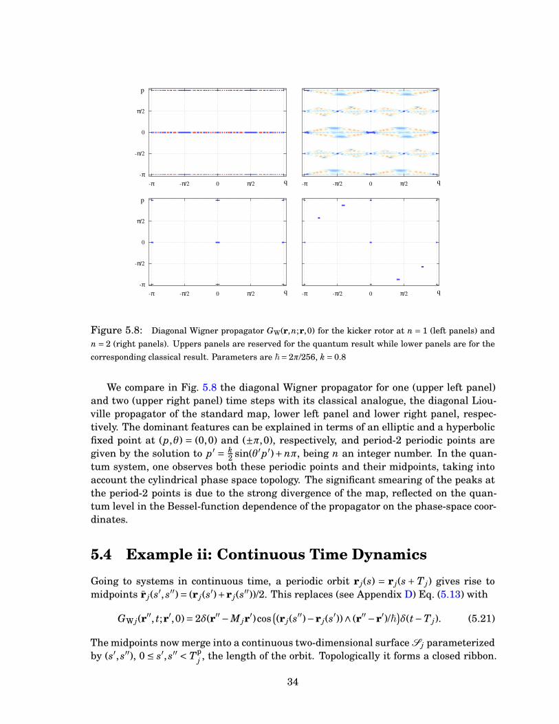
q

p

π/20-π/2-π

π/2

0

-π/2

-πq

π/20-π/2-π

q

p

π/20-π/2-π

π/2

0

-π/2

-πq π/20-π/2-π

Figure 5.8: Diagonal Wigner propagator GW(r,n;r,0) for the kicker rotor at n = 1 (left panels) and

n = 2 (right panels). Uppers panels are reserved for the quantum result while lower panels are for the

corresponding classical result. Parameters are ~= 2π/256, k = 0.8

We compare in Fig. 5.8 the diagonal Wigner propagator for one (upper left panel)and two (upper right panel) time steps with its classical analogue, the diagonal Liou-ville propagator of the standard map, lower left panel and lower right panel, respec-tively. The dominant features can be explained in terms of an elliptic and a hyperbolicfixed point at (p,θ) = (0,0) and (±π,0), respectively, and period-2 periodic points aregiven by the solution to p′ = k

2 sin(θ′p′)+nπ, being n an integer number. In the quan-tum system, one observes both these periodic points and their midpoints, taking intoaccount the cylindrical phase space topology. The significant smearing of the peaks atthe period-2 points is due to the strong divergence of the map, reflected on the quan-tum level in the Bessel-function dependence of the propagator on the phase-space coor-dinates.

5.4 Example ii: Continuous Time Dynamics

Going to systems in continuous time, a periodic orbit r j(s) = r j(s+ T j) gives rise tomidpoints r j(s′, s′′)= (r j(s′)+r j(s′′))/2. This replaces (see Appendix D) Eq. (5.13) with

GW j(r′′, t;r′,0)= 2δ(r′′−M jr

′)cos(

(r j(s′′)−r j(s

′))∧ (r′′−r′)/~)

δ(t−T j). (5.21)

The midpoints now merge into a continuous two-dimensional surface S j parameterizedby (s′, s′′), 0 ≤ s′, s′′ < Tp

j , the length of the orbit. Topologically it forms a closed ribbon.

34

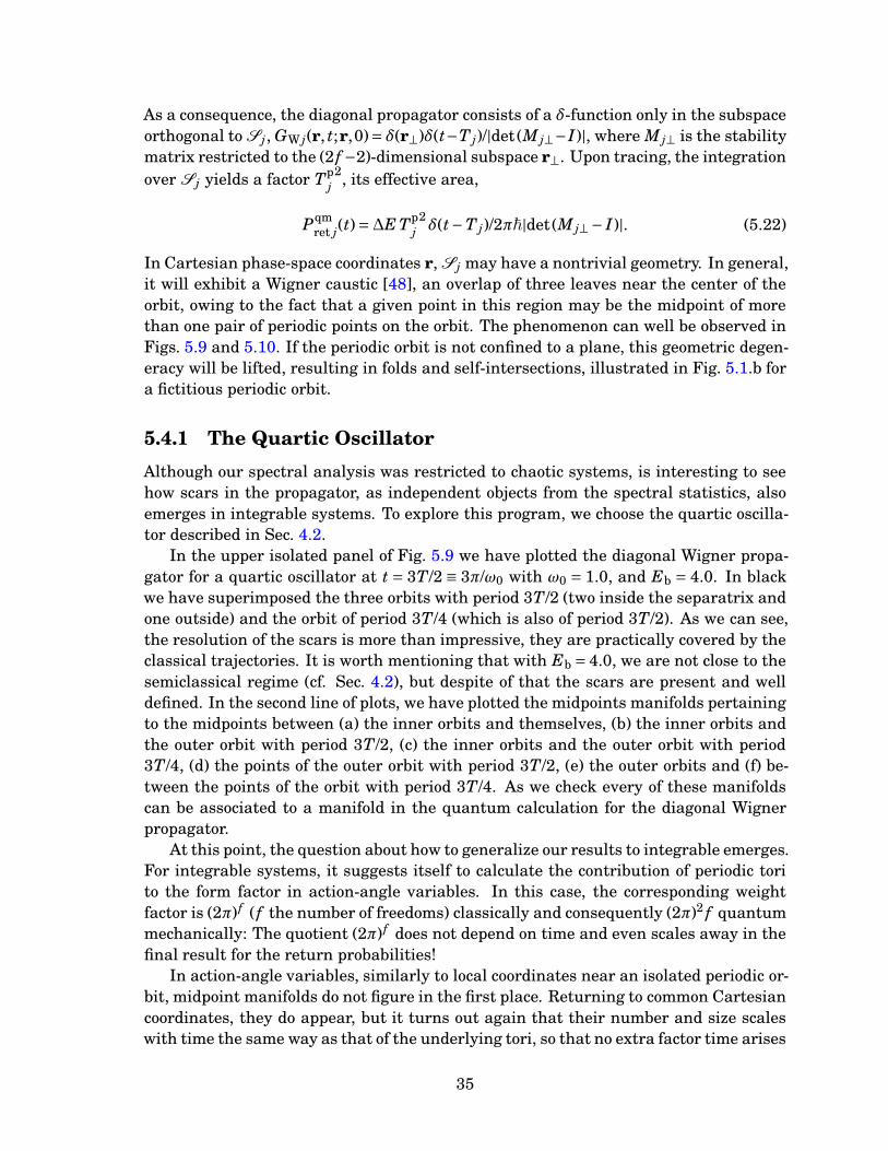
As a consequence, the diagonal propagator consists of a δ-function only in the subspaceorthogonal to S j, GW j(r, t;r,0)= δ(r⊥)δ(t−T j)/|det(M j⊥−I)|, where M j⊥ is the stabilitymatrix restricted to the (2 f −2)-dimensional subspace r⊥. Upon tracing, the integrationover S j yields a factor Tp

j2, its effective area,

Pqmret j(t)=∆E Tp

j2δ(t−T j)/2π~|det(M j⊥− I)|. (5.22)

In Cartesian phase-space coordinates r, S j may have a nontrivial geometry. In general,it will exhibit a Wigner caustic [48], an overlap of three leaves near the center of theorbit, owing to the fact that a given point in this region may be the midpoint of morethan one pair of periodic points on the orbit. The phenomenon can well be observed inFigs. 5.9 and 5.10. If the periodic orbit is not confined to a plane, this geometric degen-eracy will be lifted, resulting in folds and self-intersections, illustrated in Fig. 5.1.b fora fictitious periodic orbit.

5.4.1 The Quartic Oscillator

Although our spectral analysis was restricted to chaotic systems, is interesting to seehow scars in the propagator, as independent objects from the spectral statistics, alsoemerges in integrable systems. To explore this program, we choose the quartic oscilla-tor described in Sec. 4.2.

In the upper isolated panel of Fig. 5.9 we have plotted the diagonal Wigner propa-gator for a quartic oscillator at t = 3T/2 ≡ 3π/ω0 with ω0 = 1.0, and Eb = 4.0. In blackwe have superimposed the three orbits with period 3T/2 (two inside the separatrix andone outside) and the orbit of period 3T/4 (which is also of period 3T/2). As we can see,the resolution of the scars is more than impressive, they are practically covered by theclassical trajectories. It is worth mentioning that with Eb = 4.0, we are not close to thesemiclassical regime (cf. Sec. 4.2), but despite of that the scars are present and welldefined. In the second line of plots, we have plotted the midpoints manifolds pertainingto the midpoints between (a) the inner orbits and themselves, (b) the inner orbits andthe outer orbit with period 3T/2, (c) the inner orbits and the outer orbit with period3T/4, (d) the points of the outer orbit with period 3T/2, (e) the outer orbits and (f) be-tween the points of the orbit with period 3T/4. As we check every of these manifoldscan be associated to a manifold in the quantum calculation for the diagonal Wignerpropagator.

At this point, the question about how to generalize our results to integrable emerges.For integrable systems, it suggests itself to calculate the contribution of periodic torito the form factor in action-angle variables. In this case, the corresponding weightfactor is (2π) f ( f the number of freedoms) classically and consequently (2π)2 f quantummechanically: The quotient (2π) f does not depend on time and even scales away in thefinal result for the return probabilities!

In action-angle variables, similarly to local coordinates near an isolated periodic or-bit, midpoint manifolds do not figure in the first place. Returning to common Cartesiancoordinates, they do appear, but it turns out again that their number and size scaleswith time the same way as that of the underlying tori, so that no extra factor time arises

35

a b c

d e f

Figure 5.9: Upper isolate panel: Diagonal Wigner G(r, t;r,0) for the quartic oscillator at t = 3T/2 ≡3π/ω0, with ω0 = 1.0, and Eb = 4.0 (color code as in Fig. 5.3). In black we have superimposed the classical

trajectories having period 3T/2, which are in the center of the plot and also an orbit having period 3T/4

localized close to the borders of the plot. The resolution of the scars is impressive! In the second and

third line of plots se have plotted the midpoints manifolds (see text).

between quantum and classical return probabilities. This situation in turn reflects thefact that periodic tori form f -dimensional surfaces in phase space and are space filling,e.g., in position space, while isolated periodic orbits remain one-dimensional subsetsindependently of the number of freedoms (both for continuous time, in discrete time asimilar distinction applies). There is therefore qualitatively “more room” available formidpoint manifolds in the latter case than in the former.

5.4.2 The Harmonically Driven Quartic Oscillator

Now, by introducing a time-dependent force, Sq cos(ωt+φ), in the Hamiltonian (4.7)we generate a mixed dynamics and we get a pertinent example. In the diagonal prop-agator at t = T ≡ 2π/ω (Fig. 5.10) we identify a number of isolated peaks at periodicpoints of the classical dynamics, elliptic as well as hyperbolic, and their midpoints, andan enhancement over a well-defined region, to be interpreted as the Wigner caustic ofa period-T torus outside the frame shown, as confirms the coincidence with the corre-

36

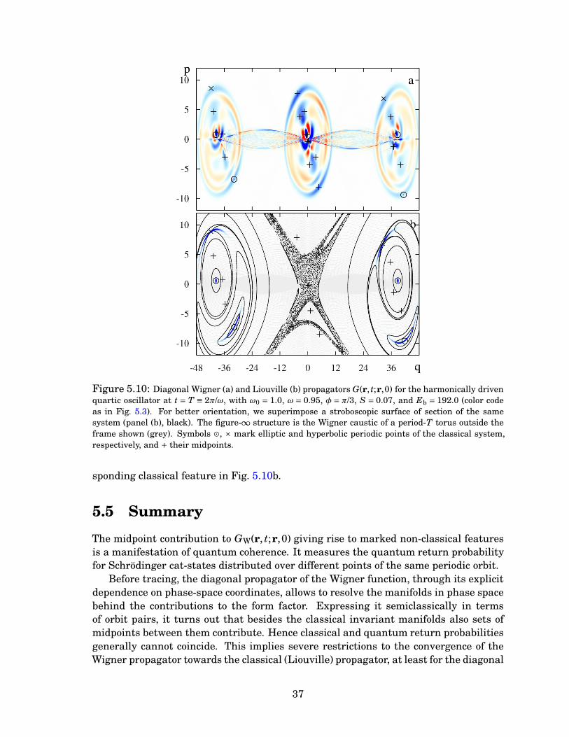
Figure 5.10: Diagonal Wigner (a) and Liouville (b) propagators G(r, t;r,0) for the harmonically drivenquartic oscillator at t = T ≡ 2π/ω, with ω0 = 1.0, ω = 0.95, φ = π/3, S = 0.07, and Eb = 192.0 (color codeas in Fig. 5.3). For better orientation, we superimpose a stroboscopic surface of section of the samesystem (panel (b), black). The figure-∞ structure is the Wigner caustic of a period-T torus outside theframe shown (grey). Symbols ¯, × mark elliptic and hyperbolic periodic points of the classical system,respectively, and + their midpoints.

sponding classical feature in Fig. 5.10b.

5.5 Summary

The midpoint contribution to GW(r, t;r,0) giving rise to marked non-classical featuresis a manifestation of quantum coherence. It measures the quantum return probabilityfor Schrödinger cat-states distributed over different points of the same periodic orbit.

Before tracing, the diagonal propagator of the Wigner function, through its explicitdependence on phase-space coordinates, allows to resolve the manifolds in phase spacebehind the contributions to the form factor. Expressing it semiclassically in termsof orbit pairs, it turns out that besides the classical invariant manifolds also sets ofmidpoints between them contribute. Hence classical and quantum return probabilitiesgenerally cannot coincide. This implies severe restrictions to the convergence of theWigner propagator towards the classical (Liouville) propagator, at least for the diagonal

37

propagator near such midpoint manifolds.That these dominant features of the diagonal Wigner propagator occur in a time-

dependent distribution function suggests calling them “time-domain scars”. By con-trast to scars in eigenfunctions, they are not affected by the uncertainty relation andtherefore allow for an unlimited resolution of classical structures.

38

CHAPTER 6

Open Quantum Systems in Configuration Space

In this Chapter we review the theory of open quantum systems in configuration space.Since an equivalent formulation is given in next Chapter, we here omit some detailsand discuss them in detail in Chapter 7.

As an application of the theory, we present the derivation of the influence-functionalfor a harmonic oscillator [8]. By means of an “artificial” relation between the propagat-ing function of the density matrix and the propagating function of the Wigner function(see Eq. (6.23)), we derive the Wigner propagating function for the damped harmonicoscillator [9]. It allows us to glimpse some of the basic ingredients of the general semi-classical theory presented in Chapter 7. In particular, we can notice that propagationis done by, in general complex, non-classical coupled pair of trajectories.

6.1 Feynman and Vernon Theory

We now turn the so far isolated quantum system S into a dissipative quantum systemby coupling it to a heat bath characterized by a temperature T. The complete Hamilto-nian then is of the general form

H = HS + HB+ HSB , (6.1)

where the second and third term describe the bath Hamiltonian and the system-bathcoupling, respectively.

As long as the complete Hilbert space is retained, the evolution of the density ma-trix is still of the form (2.11) where the system density operator ρS is replaced bythe full density operator ρ. Correspondingly, in the time evolution operator (2.10) thesystem Hamiltonian has to be replaced by the full Hamiltonian (6.1). In position rep-resentation, (2.12) still holds with the appropriate replacements. In particular thecoordinates are now Q = {q,Q} and comprise the system coordinate q, for simplicity wetake here system S being 1-D, as well as the vector of bath coordinates Q.

39

For a dissipative system, one is usually not interested in the full dynamics but onlyin the reduced dynamics of the system degree of freedom. In order to integrate out thebath degrees of freedom, one needs to specify the initial density matrix of system andbath. One possibility is to neglect initial correlations between system and bath and toemploy factorizing initial conditions. Then, the initial density matrix is given by theproduct of a density matrix of the system and the thermal density matrix of the heatbath. In position representation, the full initial density matrix reads (see Appendix Efor a more general treatment)

ρ(Q′+,Q′

−,0)= ρS(q′+, q′

−,0)ρB(Q′+,Q′

−,0) . (6.2)

The time evolution of the initial state (6.2) is obtained as a generalization of theconsiderations in Sect. 2.3 by substituting the single system degree of freedom by theensemble of system and bath degrees of freedom. In order to obtain the reduced dynam-ics of the system, one needs to trace out the environmental degrees of freedom. Thiscan be done analytically if the heat bath is modeled by a set of harmonic oscillatorswith masses m j and frequencies ω j whose coordinates are bilinearly coupled to thesystem coordinate. The Hamiltonian (6.1) then consists of the three contributions

HS =p2

2m+V (q) , (6.3)

HB =∞∑

j=1

1

2m jP2

j +1

2m jω

2jQ

2j , (6.4)

HSB =−q∞∑

j=1c jQ j + q2

∞∑

j=1

c2j

2m jω2j

, (6.5)

where c j are the coupling constants. The second term in (6.5) corrects a potentialrenormalization induced by the coupling of the system to the heat bath. Tracing outthe heat bath, one finds for the time evolution of the initial state (6.2)

ρS(q′′+, q′′

−, t)=∫

dq′+dq′

−J(q′′+, q′′

−, t; q′+, q′

−)ρS(q′+, q′

−,0) , (6.6)

where we have introduced the propagating function J(q′′−, q′′

+, t; q′+, q′

−), which can beexpressed in terms of a path integral over the system degree of freedom as

J(q′′−, q′′

+, t; q′+, q′

−)=∫

Dq+Dq−exp(

i

~(SS[q+]−SS[q−])

)

F [q+, q−] . (6.7)

The action SS is the action related to the system Hamiltonian (6.3). The influence ofthe heat bath in (6.7) is contained in the influence-functional

F [q+, q−]= exp(Φ[q+, q−]) , (6.8)

40

with

Φ[q+, q−]=i

~

m

2

[

(q′++ q′

−)∫t

0dsγ(s)[q+(s)− q−(s)]

+∫t

0ds

∫s

0duγ(s−u)[q+(u)+ q−(u)][q+(s)− q−(s)]

]

+1

~

∫t

0ds

∫s

0du[q+(u)− q−(u)]αR(u− s)[q+(s)− q−(s)], (6.9)

where the noise kernel αR(s) and damping kernel are defined in terms of the micro-scopic quantities of the heat bath and its coupling to the system through the spectraldensity of bath oscillators [7,8]

I(ω)=π∞∑

j=1

c2j

2m jω jδ(ω−ω j) , (6.10)

in the following way,

αR(s)=∫∞

0

dω

ωcoth

(

ω~

2kBT

)

cos(ωs)I(ω), (6.11)

wherein kB denotes the Boltzmann constant and T the temperature of the bath. Thefriction kernel γ(s) in terms of the spectral density reads

γ(s)= 2

m

∫∞

0

dω

π

I(ω)

ωcos(ωs). (6.12)

At this point is illustrative to compare (6.7) with the equivalent path-integral ex-pression of (2.13)

J(q′′−, q′′

+, t; q′+, q′

−)=∫

Dq+Dq−exp(

i

~(SS[q+]−SS[q−])

)

, (6.13)

where we note that in the dissipative case trajectories q± are coupled by the influencefunctional F [q+, q−], this generates that the evolution of the relevant propagating tra-jectories, as we will see in next section, do not correspond to the classical one. In thefollowing, we present the derivation of the influence-functional for the interesting casea harmonic oscillator [8] and introduce the basic features of propagation in phase-spaceof dissipative systems developed in next Chapter.

6.2 Quantum Damped Harmonic Oscillator

While the results reviewed in the previous section are valid for a general system degreeof freedom, we will now specifically consider a damped harmonic oscillator with

V (q)= m

2ω2

0 q2 . (6.14)

41

As for the propagator in the unitary case, the path-integral expression for the propa-gating function (6.7) is evaluated by an expansion around the paths maximizing thecomplex action. The dependence on the initial and final coordinates is entirely deter-mined by these paths while the fluctuations only yield a time-dependent prefactor. Fora harmonic oscillator, the complex action in (6.7) is stationary for trajectories satisfy-ing [140]

mq±(s)+mω20q±(s)∓

1

2m

d

ds

∫t

sduγ(s−u)[q+(u)− q−(u)]

+ 1

2m

d

ds

∫s

0duγ(s−u)[q+(u)+ q−(u)]= i

∫t

0duαR(s−u)[q+(u)− q−(u)].

(6.15)

The paths are subject to the boundary conditions q±(0)= q′±, q±(t)= q′′

±.In (6.15) the trajectories are driven by the same imaginary nonlocal force so that

they are affected by decoherence in the same way. For linear systems, it turns out thatthe imaginary part of the trajectories does not need to be considered and that the realpart of the trajectories is sufficient to obtain the propagating function [140,141]. From(6.15) one finds that the equations of motion of the two paths q+ and q− differ. As weshall see in the sequel, neither of the two paths follows a classical equation of motionand their separation grows exponentially fast. This somewhat surprising behavior is aconsequence of the coupling to the heat bath.

In order to render the discussion of the trajectories more transparent, in the fol-lowing we assume Ohmic damping, i.e. I(ω) = mγω and γ(t) = 2γδ(t), the equations ofmotion (6.15) reduce to

q±+ω20q±+γq∓ = 0 , (6.16)

where the damping constant couples the trajectories q+ and q−. It is interesting tonote that γq∓ acts actually as a driving instead of a damping in the sense that theseparation between trajectories grows exponentially (see Fig. 6.1). This can be seenmore clearly by decoupling the two equations of motion, using the half–sum coordinateq = (q++ q−)/2 and the difference coordinate q = q+− q−. The equations (6.16) thenread

q+γq+ω20q = 0

¨q−γ ˙q+ω20 q = 0 .

(6.17)

The half-sum-coordinate trajectory corresponding to the paths q+ and q− obeysthe classical equation of motion, which here takes a time-local form because we haveassumed Ohmic damping. In contrast to the sum coordinate q which decreases expo-nentially in time, the difference coordinate q grows exponentially so that we obtain ahyperbolic dynamics in the (q, q)-plane. As a consequence, the trajectories q± do notobey the classical damped equation of motion. The solutions of the equations of motion(6.17) read

q(s)= q′G−(t− s)

G−(t)+ q′′G+(s)

G+(t),

q(s)= q′G+(t− s)

G+(t)+ q′′G−(s)

G−(t),

(6.18)

42

where

G±(t)=1

ωdexp

(

∓γ

2t)

sin(ωdt) (6.19)

and ω2d = ω2

0 −γ2/4. We remark that by choosing appropriate functions G±(t), moregeneral linear damped system like the parametrically driven damped harmonic oscil-lator [10,142] can be studied with solutions of the form (6.18).

We now return to the propagating function which was given in (6.7) in terms of atowfold path integral. It is instructive to decompose the exponent into two parts

S(q′′, q′′, t; q′, q′)= S1 +S2 , (6.20)

where

S1 = m[

(q′ q′+ q′′ q′′)G+(t)

G+(t)− q′ q′′ 1

G−(t)− q′′ q′ 1

G+(t)

]

(6.21)

is obtained by evaluating the action of the system degree of freedom along the trajecto-ries given by (6.18) while

S2 =i

2

∫t

0ds

∫t

0duαR(s−u)q(s)q(u) (6.22)

arises from the influence functional (6.8), i.e. by the interaction of paths at differenttimes through the coupling to the environment. The significance of this decompositionwill become clear in the following section where we discuss the results of the presentsection from a phase-space point of view.

6.2.1 Damped Harmonic Oscillator in Phase Space

The unitary time-evolution of the Wigner function Sec. (2.3) can immediately be trans-ferred to the dissipative case if we relate the Wigner propagating function to the prop-agating function by means of

GW(r′′, t;r′,0)=1

2π~

∫

dq′dq′′exp(

i

~p′ q′−

i

~p′′ q′′

)

J(q′′, q′′, t; q′, q′) . (6.23)

Before analyzing the Wigner propagating-function for Ohmic damping, we discussthe decomposition (6.20) of the exponent of the propagating function. The contribution(6.21) is linear in the difference coordinates q′ and q′′. Performing the transformation(6.23), we therefore arrive at the Wigner propagating-function

GW(r′′,r′)= δ(

r′′−rcl(r′, t))

, (6.24)

where the classical phase-space trajectory

pcl(t)= G+(t)p′+m(

G2+(t)

G+(t)− 1

G−(t)

)

q′,

qcl(t)=G+(t)

mp′+ G+(t)q′,

(6.25)

43

with G±(t) defined by (6.19) is now damped. While (6.25) satisfies qcl(0) = q′ as ex-pected, the initial momentum is given by pcl(0) = p′−mγq′. This initial slip is typicalfor factorizing initial conditions [140].

Employing the Wigner propagating function (6.24) amounts to adding a velocity-dependent force in the system Hamiltonian as was proposed by Caldirola and Kanai(see e.g. the review [59] for a description of this kind of phenomenological approaches).However, the Wigner propagating function (6.24) accounts only for part of the exponentof the propagating function. The second contribution (6.22) is quadratic in the differ-ence coordinate and limits their contributions. As a result, the delta function in (6.24)will be broadened into a Gaussian

GW(r′′, t;r′)= m

2π~Λ(t)1/2

∣

∣

∣

∣

G+(t)

G+(t)

∣

∣

∣

∣

exp{

− 1

2~Λ(t)

(

r′′−rcl(t))

Σ

(

r′′−rcl(t))T

}

, (6.26)

whose center moves along the damped classical trajectory (6.25). The matrix appearingin the exponent is given by its components

Σ11 = a(t)

Σ12 =Σ21 =−mG+(t)

G+(t)[a(t)+b(t)]

Σ22 = m2 G2+(t)

G2+(t)

[a(t)+2b(t)+ c(t)]

(6.27)

and Λ(t)= det(Σ)/m2 = a(t)c(t)−b(t)2. The functions

a(t)= G2+(t)Ψ(t, t)

b(t)= G+(t)G+(t)∂Ψ(t, t′)

∂t

∣

∣

∣

∣

t′→t−

c(t)=G2+(t)

∂2Ψ(t, t′)

∂t∂t′

∣

∣

∣

∣

t′→t−

(6.28)

can all be expressed in terms of a single function

Ψ(t, t′)=∫t

0ds

∫t′

0duK ′(s−u)

G+(t− s)

G+(t)

G+(t′−u)

G+(t′). (6.29)

This function is completely determined by the thermal position autocorrelation func-tion ⟨q(t)q(0)⟩ and its time derivatives, the interested reader may also want to consultRef. [140] for further details.

The Gaussian form of the Wigner propagating function (6.26) is a consequence ofthe linearity of the harmonic oscillator damped by the coupling to a harmonic heat bath.A similar expression has therefore be found in the Markovian limit [66]. Similarly, theresult could be generalized to the case of non-factorizing initial conditions which wouldalso yield a Gaussian.

From (6.23) it follows that pairs of trajectories q± satisfying the equations of motion(6.16) and leading to a half-sum-coordinate motion from the initial phase-space point r′

44

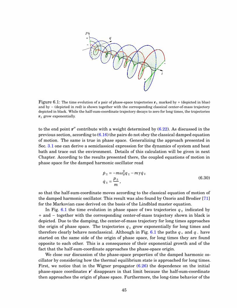
p

q

t

+

–

+

–

Figure 6.1: The time evolution of a pair of phase-space trajectories r± marked by + (depicted in blue)and by − (depicted in red) is shown together with the corresponding classical center-of-mass trajectorydepicted in black. While the half-sum-coordinate trajectory decays to zero for long times, the trajectoriesr± grow exponentially.

to the end point r′′ contribute with a weight determined by (6.22). As discussed in theprevious section, according to (6.16) the pairs do not obey the classical damped equationof motion. The same is true in phase space. Generalizing the approach presented inSec. 3.1 one can derive a semiclassical expression for the dynamics of system and heatbath and trace out the environment. Details of this calculation will be given in nextChapter. According to the results presented there, the coupled equations of motion inphase space for the damped harmonic oscillator read

p± =−mω20q±−mγq∓

q± =p±m

,(6.30)

so that the half-sum-coordinate moves according to the classical equation of motion ofthe damped harmonic oscillator. This result was also found by Ozorio and Brodier [71]for the Markovian case derived on the basis of the Lindblad master equation.

In Fig. 6.1 the time evolution in phase space of two trajectories q± indicated by+ and − together with the corresponding center-of-mass trajectory shown in black isdepicted. Due to the damping, the center-of-mass trajectory for long times approachesthe origin of phase space. The trajectories q± grow exponentially for long times andtherefore clearly behave nonclassical. Although in Fig. 6.1 the paths q+ and q− havestarted on the same side of the origin of phase space, for long times they are foundopposite to each other. This is a consequence of their exponential growth and of thefact that the half-sum-coordinate approaches the phase-space origin.

We close our discussion of the phase-space properties of the damped harmonic os-cillator by considering how the thermal equilibrium state is approached for long times.First, we notice that in the Wigner propagator (6.26) the dependence on the initialphase-space coordinates r′ disappears in that limit because the half-sum-coordinatethen approaches the origin of phase space. Furthermore, the long-time behavior of the

45

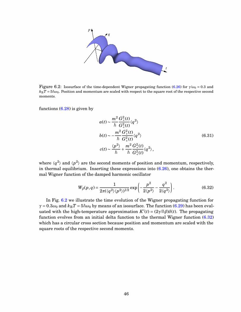
p

q

t

Figure 6.2: Isosurface of the time-dependent Wigner propagating function (6.26) for γ/ω0 = 0.3 andkBT = 5~ω0. Position and momentum are scaled with respect to the square root of the respective secondmoments.

functions (6.28) is given by

a(t)∼ m2

~

G2+(t)

G2+(t)

⟨q2⟩

b(t)∼−m2

~

G2+(t)

G2+(t)

⟨q2⟩

c(t)∼⟨p2⟩~

+m2

~

G2+(t)

G2+(t)

⟨q2⟩ ,

(6.31)

where ⟨q2⟩ and ⟨p2⟩ are the second moments of position and momentum, respectively,in thermal equilibrium. Inserting these expressions into (6.26), one obtains the ther-mal Wigner function of the damped harmonic oscillator

Wβ(p, q)=1

2π(⟨q2⟩⟨p2⟩)1/2exp

(

−p2

2⟨p2⟩−

q2

2⟨q2⟩

)

. (6.32)

In Fig. 6.2 we illustrate the time evolution of the Wigner propagating function forγ= 0.3ω0 and kBT = 5~ω0 by means of an isosurface. The function (6.29) has been eval-uated with the high-temperature approximation K ′(t) = (2γ/~β)δ(t). The propagatingfunction evolves from an initial delta function to the thermal Wigner function (6.32)which has a circular cross section because position and momentum are scaled with thesquare roots of the respective second moments.

46

CHAPTER 7

Open Quantum Systems in Phase Space

In this Chapter we construct the theory of quantum open systems in phase space. Toachieve this, we first make use of Marinov’s path integrals in phase space to translatethe Feynman and Vernon approach into phase-space language and then derive theexpression for the propagating function in phase space assuming a Ullerma-Caldeira-Leggett model for the bath. Once we get those expressions we can proceed to evaluatethe path integrals by the use of semiclassical approximations. It allows us to calculatethe dissipative version of the Wigner propagator presented in Sec. 3.1.

7.1 Feynman and Vernon Theory in Phase Space

Let S and B be two interacting systems and denote by f and F their respective free-doms. Likewise, let H(r,R) be the Hamiltonian of the total systems defined by (6.1)and let be

HW(r,R)= HW,S(r)+HW,B(R)+HW,SB(r,R), (7.1)

its corresponding Weyl symbol. In last expression, HW,S(r) and HW,B(r) denote theHamiltonian of system S and system B, respectively, while HW,SB(r,R) is the interac-tion Hamiltonian; r= (q1, q2, · · · , q f , p1, p2, · · · , p f ) and R= (Q1,Q2, · · · ,QF ,P1,P2, · · · ,PF)denote generic points in the phase space of S and B, respectively.

As in the configuration-space description, under appropriate replacements, we canstudy the dynamics of the total Hamiltonian HW(r,R) using the expression for uni-tary time-evolution. In this case, we calculate the Wigner propagator of the total sys-tem based on the path-integral description given in Sec. (2.3.2), in order to make useof (2.28) we define R = (q1, q2, · · · , q f ,Q1,Q2, · · · ,QF , p1, p2, · · · , p f ,P1,P2, · · · ,PF) withboundary conditions R(0)=R

′ and R(t)=R′′. In this way we get

GW(R′′, t;R′,0)=1

h(f+F)

∫

D2(f+F)

R

∫

D2(f+F)

R exp{

−i

~S

[

{R}, {R}, t]

}

, (7.2)

47

where R can be considered as a fluctuation without restriction around of the trajectoryR(τ) while DR and DR denote an infinity product of measures in the total phase spaceand S the action of the total system, S = SS+SB+SSB given by

S[{R}, {R}, t]=∫t

0dτ

[

R∧R+HW

(

R+1

2R

)

−HW

(

R−1

2R

)]

, (7.3)

This allows us to express the time evolution of the total Wigner function as

ρW(R′′, t)=∫

d2(f+F)R

′

(2π~)(f+F)

R(t)=R′′

∫

R(0)=R′

D2(f+F)

R

∫

D2(f+F)

R exp{

− i

~S

[

{R}, {R}, t]

}

ρW(R′,0),

or, equivalently, in terms of the coordinates of the subsystems as,

ρW(R′′,r′′, t)=∫

d2F R′

(2π~)F

d2 f r′

(2π~) f

r(t)=r′′∫

r(0)=r′

D2 f r

∫

D2 f r

R(t)=R′′∫

R(0)=R′

D2F R

∫

D2F R

×exp{

−i

~

[

SS [{r}, {r}, t]+SB[

{R}, {R}, t]

+SSB[

{r}, {r}, {R}, {R}, t]]

}

ρW(R′,r′,0).

(7.4)

If at t = 0 the subsystems S and B are uncorrelated, i.e. if we can express the initialWigner function as ρW(R′,r′,0)= ρW,S(r′,0)ρW,B(R′,0), we can write

ρW(r′′, t)=∫

dF R′′ρW(R′′,r′′, t)=∫

d2 f r′JW(r′′, t;r′,0)ρW,S(r′,0). (7.5)

with JW(r′′, t;r′,0), the propagating function of the Wigner function, defined by

JW(r′′, t;r′,0)=1

h f

r(t)=r′′∫

r(0)=r′

Df r

∫

Df rexp

{

−i

~SS [{r}, {r}, t]

}

FW [{r}, {r}, t] , (7.6)

where

FW [{r}, {r}, t]=1

hF

∫

d2F R′′∫

d2F R′WB(R′,0)

R(t)=R′′∫

R(0)=R′

D2F R

∫

D2F R

×exp{

−i

~

[

SB[

{R}, {R}, t]

+SSB[

{r}, {r}, {R}, {R}, t]]

}

,

(7.7)

is the influence functional in phase space. In what follows we omit the subscript W forthe Hamiltonians.

Although, at this point we could be tempted to introduce semiclassical approxi-mations for the evolution of the dissipative system, e.g. considering stationary-phaseapproximation for the influence functional JW(r′′, t;r′,0) or to the total Wigner propa-gator GW(R′′, t;R′,0), it is very premature because dissipation is achieved just when

48

the number of freedoms of the bath tends to infinity, F →∞. Otherwise what we willfind again is the result for Hamiltonian systems derived in [1]. For this reason, semi-classical limit will be discussed later.

7.2 Ullersma-Caldeira-Leggett Model in Phase Space

Following the Ullersma’s ideas [60], we couple linearly a single freedom, for simplicity,to a thermal bath modeled by a collection of harmonic oscillators, explicitly

HS(r)=p2

2m+V (q), (7.8)

HB(R)=F∑

j=1

1

2m jP j

2 +1

2m jω

2jQ

2j , (7.9)

HSB(r,R)=−qF∑

j=1c jQ j + q2

F∑

j=1

c2j

2m jω2j

. (7.10)

We note that by difference to (6.3), here we do not deal with operators but with c-function. The equations of motion for each bath mode read

P j =−m jω2jQ j + c j q, Q j =

P j

m j, (7.11)

and for the central system freedom we have

p =−∂V

∂q+

F∑

j=1c jQ j − q

F∑

j=1

c2j

m jω2j

, q =p

m, (7.12)

with the aim of constructing the Ullersma-Caldeira-Leggett model in phase space wefirst derive the Wigner propagator for the total system (see Appendix F for the detailedcalculation),

GW(r′′,R′′j , t;r′,R′

j,0)= 1

h

r(t)=r′′∫

r(0)=r′

Dr

∫

Drexp(

− i

~SS[{r}, {r}, t]

)

×F∏

j=1δ

(

P ′′j −Pcl

j (P ′j,Q

′j, t)

)

δ(

Q′′j −Qcl

j (P ′j,Q

′j, t)

)

(7.13)

×exp

{

i

~

[

c j

∫t

0dt′Qcl

j (P ′j,Q

′j, t′)q(t′)−

c2j

m jω2j

∫t

0dt′q(t′)q(t′)

]}

,

where

SS[{r}, {r}, t]=∫t

0dt′

[

r∧ r+HS

(

r+ 1

2r

)

−HS

(

r− 1

2r

)]

, (7.14)

49

with Pclj (P ′

j,Q′j, t) and Qcl

j (P ′j,Q

′j, t) being the classical equation of motion given by the

solution of (7.11). Eq. (7.13) is the Wigner propagator of an arbitrary system S coupledto a set of F-harmonic oscillators. As is expected, the Wigner propagator is a δ-functionalong the classical trajectory in the phase-space components of the bath. The last linein Eq. (7.13) incorporate the interaction between S and B while the first line describesthe isolated version of system S.

7.3 Semiclassical Approximation

In this section we provide two semiclassical approximations for the Wigner propagatorusing two different approaches.

7.3.1 Semiclassical Approximation: Langevin Trajectories Ap-

proach

In this subsection we derive the semiclassical Wigner propagator base on the Hamil-tonian expression (7.13). To do that we have to go back to the discrete version (F.6)and calculate the stationary trajectories of the action along each freedom of the totalsystem,

p =− ∂

∂q

(

H(r+ 1

2r)−H(r− 1

2r)

)

+F∑

j=1c jQ j − q

F∑

j=1

c2j

2m jω2j

, (7.15)

˙p =− ∂

∂q

(

H(r+ 1

2r)−H(r− 1

2r)

)

+F∑

j=1c jQ j − q

F∑

j=1

c2j

2m jω2j

, (7.16)

q =∂

∂p

(

H(r+1

2r)−H(r−

1

2r)

)

, ˙q =∂

∂p

(

H(r+1

2r)−H(r−

1

2r)

)

. (7.17)

P j =−m jω2jQ j − c j q, Q j = P j/m j,

˙P j =−m jω2jQ j − c j q, ˙Q j = P j/m j. (7.18)

Introducing a new set of coordinates, r± = r± r/2 and R j,± =R j ± R j/2, we have

p± =−∂H(r±)

∂q±+

F∑

j=1c jQ j,±− q±

F∑

j=1

c2j

2m jω2j

, q± =p±m

, (7.19)

P j,± =−m jω2jQ j,±− c j q±, Q j,± = P j,±/m j (7.20)

Eqs. (7.20) can be solved analytically assuming that q± is an arbitrary function oft [143], after integrating by parts, we obtain

p±+ ∂H(r±)

∂q±+

∫t

0dt′γ(t− t′)q±(t′)= ξ±(t), (7.21)

50

with the damping kernel, γ(t) = 1m

∑Fj=1

c2j

m jω2jcosω j t, and the operator-valued fluctuat-

ing forces

ξ±(t)=F∑

j=1c j

[(

Q′j,±−

c j

m jω2j

q′±

)

cosω j t+P ′

j,±m jω j

sinω j t

]

. (7.22)

An important feature of (7.21) is that the trajectories r+ and r− evolve independently,as in the unitary case. As we can see, these two fluctuating forces are independent, butthey obey the same statistic. The fluctuating forces vanish if averaged over a thermaldensity matrix of the environment including the coupling to the system [143]

⟨ξ±(t)⟩B+SB =TrB

[

ξ±(t)exp(

−β(HB+HSB))]

TrB[

exp(

−β(HB +HSB))] = 0 , (7.23)

where β= 1/kBT, being kB the Boltzmann constant and T the temperature. For weakcoupling, one may want to split off the transient term mγ(t)q′

± which is of second orderin the coupling and write the fluctuating force as [144]

ξ±(t)= ζ±(t)−mγ(t)q′± . (7.24)

The so defined force ζ±(t) vanishes if averaged over the environment alone

⟨ζ±(t)⟩B =TrB

[

ζ±(t)exp(−βHB)]

TrB[

exp(−βHB)] = 0 . (7.25)

An important quantity to characterize the fluctuating force is the correlation func-tion which again can be evaluated for ξ± with respect to HB +HSB or equivalently forζ± with respect to HB alone,

⟨ζ±(t)ζ±(0)⟩B =∑

j,lc jcl

⟨(

Q′j,± cos(ω j t)+

P ′j,±

m jω jsin(ω j t)

)

Q′l,±

⟩

B

. (7.26)

In thermal equilibrium the second moments are given by [143]

⟨

Q′j,±Q′

l,±

⟩

B= δ jl

~

2m jω jcoth

(

~βω j

2

)

, (7.27)

⟨

P ′j,±Q′

l,±

⟩

B=−

i~

2δ jl , (7.28)

so that the noise correlation function finally becomes

⟨ζ(t)±ζ(0)±⟩B =F∑

j=1

~c2j

2m jω j

[

coth(

~βω j

2

)

cos(ω j t)− isin(ω jt)]

. (7.29)

The imaginary part appearing here is a consequence of the fact that the operatorsζ(t)± and ζ(0)±, in general, do not commute. The correlation function (7.29) appears asintegral kernel for the evolution of the reduced density matrix, which will be derived

51

in the next section. It is remarkable that within a reduced description for the systemalone all quantities characterizing the environment may be expressed in terms of the

spectral density of bath oscillators I(ω) = π∑F

j=1

c2j

2m jω jδ(ω−ω j) . As an example, the

damping kernel may be expressed in terms of this spectral density as [7,8]

γ(t)=1

m

F∑

j=1

c2j

m jω2j

cos(ω j t)=2

m

∫∞

0

dω

π

I(ω)

ωcos(ωt) . (7.30)

and the correlation ⟨ζ(t)±ζ(0)±⟩B as

αL(t)= ⟨ζ±(t)ζ±(0)⟩B = ~

∫∞

0

dω

πI(ω)

[

coth(

~βω

2

)

cos(ωt)− isin(ωt)]

. (7.31)

For practical calculations, it is therefore unnecessary to specify all parameters m j,ω j

and c j. It rather suffices to define the spectral density I(ω).In order to construct a semiclassical theory based on (7.13) we have to note that γ(t)

depends exclusively on the parameter of the bath modes and not on the dynamics, ad-ditionally ξ±(t) depends only on a summation of the initial condition of the bath modesand not on the evolution of each mode. Assuming that the initial Wigner function ofthe total system can be written as W(r′,0)WB(R′

1,R′2, . . .R′

F ,0), the former argumentsallows us to take q±(t) again as a given function, evolve the bath modes and averageover them, this ends up with the following expression for the propagating function ofthe Wigner function

G(r′′, t;r′,0)=⟨

1

h

∫

Dr

∫

Drexp{

−i

~S

S[{r}, {r}, t]}⟩

. (7.32)

where ⟨·⟩ denotes average over all the possible realizations of the stochastic processesξ(t)± and S

S given by

SS[{r}, {r}, t]= SS[{r}, {r}, t]+

∫t

0dt′

∫t′

0dt′′γ(t′− t′′) ˙q(t′′)−

∫t

0dt′ξ(t′)q(t′). (7.33)

An important feature of (7.32) is that all realizations evolve unitarily. In order to gen-erate the thermal noise one can make use of the numerical strategy developed in [145],which has the advantage that the thermal noise is introduced in the time domain with-out prior knowledge of bath modes. The semiclassical expression of (7.32) implies theevaluation of (7.33) along the stochastic trajectories given by (7.21) and a sum overtrajectories r±, since any coupling between trajectories is present in the equation ofmotion, then the functional form of semiclassical expression is basically the same as(3.5). We restrict the formal derivation of the semiclassical expression of the propa-gating function for the next section using an equivalent formulation yet not stochasticand here only note that semiclassics can also be introduced in the correlation functionperforming an expansion up second order around ~= 0, this correlation function in the

52

Ohmic case, I(ω)= mγω, reduces to the real-valued expression

αL(t)= mkBTγ(t)−mβ~2

12γ(t)+O (~3) , (7.34)

where γ(t) = 2γδ(t). The first term on the right hand side corresponds to the classicalnoise correlation function [146], while the second term accounts for the first quantumcorrections.

With this approach we have that propagation could be done by independent stochas-tic trajectory pairs. This kind of approach is in the spirit of the Langevin equationand was used in [147, 148] to provide a quantum stochastic theory of dissipation andin [67] to construct a kind of Herman-Kluk propagator for non-Markovian dissipa-tive processes. However, one has to be careful with results from these approachesbecause as has been discussed in [149], pure-state quantum trajectories for generalnon-Markovian systems do not exist.

7.3.2 Semiclassical Approximation: Reduced density matrix ap-

proach

In this section, we shall assume that initial Wigner function of the total system can bewritten as ρW(r′,0)ρW,B(R′

1,R′2, . . .R′

F ,0). Additionally, as in the last case, we assumethat the environment is initially in thermal equilibrium at temperature T, it meansthat the Wigner function of the bath can be written as

ρW,B(R′1,R′

2, . . .R′F ,0)=

F∏

j=1ρW, j(P

′j,Q

′j,0) (7.35)

where

ρW, j(P′j,Q

′j,0)=

1

π~tanh

(

~βω j/2)

exp(

−tanh

(

~βω j/2)

m jω j~(P ′2

j +m2jω

2jQ

′2j )

)

. (7.36)

Under these assumptions, we can perform the integrations over P j and Q j and takethe trace over the bath coordinates. Before proceeding it is worth mentioning thatMagalinskii [150] was the first in noticing that the elimination of the environmentaldegrees of freedom leads indeed to a damped equation of motion for the system coordi-nate. So, we have that within this approach the influence functional FW [{r}, {r}, t] in(7.7) is given by

FW[{r}, {r}, t]= exp

{

−i2µ

~

∫t

0dt′q(t′)q(t′)− i

2

~

∫t

0dt′

∫t′

0dt′′αI(t

′− t′′)q(t′′)q(t′)

−1

~

∫t

0dt′

∫t′

0dt′′αR(t′− t′′)q(t′′)q(t′)

}

, (7.37)

53

where

µ=F∑

j=1

c2j

2m jω2j

, αI(t′− t′′)=−

F∑

j=1

c2j

2m jω jsinω j(t

′− t′′) (7.38)

and

αR(t′− t′′)=F∑

j=1

c2j

2m jω jcoth

(

~ω jβ

2

)

cosω j(t′− t′′). (7.39)

Expression (7.37), in appropriate coordinates of difference and half-sum, coincides withthe standard result [7,8,58]. At this point we cannot talk about dissipation yet becausean important step is left, the evaluation of F → ∞. In order to achieve that, let usdescribe the continuum of harmonic oscillators, as in the previous approach, by thespectral distribution I(ω),

α(t)=αR(t)+ iαI(t)=1

π

∫∞

0dωI(ω)

(

coth(

~ωβ

2

)

cosωt− isinωt)

=1

~αL(t). (7.40)

The imaginary part αI(t) of the Feynman-Vernon kernel is related to the dampingkernel γ(t) of the classical equation of motion of this model [58],

αI(t)=m

2

dγ(t)

dt, (7.41)

so we have that

JW(r′′,r′, t)= 1

h

r(t)=r′′∫

r(0)=r′

Dr

∫

Drexp(

− i

~SS[{r}, {r}, t]

)

exp

{

−i2µ

~

∫t

0dt′q(t′)q(t′)− i

m

~

∫t

0dt′

∫t′

0dt′′

dγ(t′− t′′)

d(t′− t′′)q(t′′)q(t′)

− 1

~

∫t

0dt′

∫t′

0dt′′αR(t′− t′′)q(t′′)q(t′)

}

, (7.42)

is the propagator of the Wigner function for non-Markovian dissipative system in theCaldeira-Leggett approach. From this expression we can see that symplectic symmetryis broken, it comes from the choice of the coupling term, the central system is coupledto the bath just in the position, q−coupling. To recover this symmetry one should intro-duce a similar coupling in the momenta, i.e., a coupling term of the form

∑Fj=1 r∧C jR j,

with C j =(

0 CqQ, j

CpP, j 0

)

. However, in this case the behavior is qualitative very sim-

ilar to the one in absence of p-coupling [151, 152]. If we would introduce independentbaths for q and p−couplings, we have to deal with some extra phenomena, e.g., a kindof semiclassical frustration of dissipation which is characterized by underdamped oscil-lations and longer relaxation times in the strong coupling regime which is generated

54

because of the canonically conjugate character of position and momentum [151, 152].We have omitted the mixed coupling terms CqP, j qP j and CpQ, j pQ j because, by meansof canonicals transformations they can be seen as couplings in positions and momenta,respectively, plus a harmonic shift of the potential [8]. So, the breaking of the symplec-tic geometry is well justified and we can guarantee that the basic features of quantumdissipation are encoded in (7.42).

We shall derive now the paths which maximize the complex action of the propaga-tor (7.42) and the semiclassical expression of the propagating function of the Wignerfunction. In order to gain physical intuition let us start with the simplest case, Ohmicdissipation at high temperatures.

Semiclassical Ohmic Approximation at High Temperatures

At high temperatures, Ohmic dissipation is characterized by the memoryless kernels[58]

γ(t′− t′′)= 2γδ(t′− t′′), αR(t′− t′′)= 2mγ

~βδ(t′− t′′), (7.43)

this choice of the kernels leaves a sort of Markovian approximation. Under these par-ticular conditions the Wigner propagator takes the form

JW(r′′,r′, t)= 1

h

r(t)=r′′∫

r(0)=r′

Dr

∫

Drexp(

− i

~SS[{r}, {r}, t]

)

(7.44)

exp{

−i2γm

~q′

∫t

0dt′δ(t′)q(t′)− i

mγ

~

∫t

0dt′ q(t′)q(t′)−

mγ

β~2

∫t

0dt′ q(t′)2

}

,

where we have used the arbitrariness of µ and fixed it to be defined by µ = mγδ(0)[8, 58]. The presence of the term containing δ(t′) introduces a discontinuity at t = 0, itcomes from the fact that we have assumed factorizing initial conditions for the Wignerfunction. Such discontinuity is a well-known fact and can be removed considering someinitial correlations between the central system and the bath [143].

The next step in our program is the application of the stationary-phase approxima-tion, however we have to be careful because of the presence of the imaginary term inthe action. For this reason, we first consider when the stationary-phase approximationcan be done only with the real phase. We can rewrite the non-Hamiltonian phase in(7.44) as −i

∫t0 dt′[2γm

~q′δ(t′)q(t′)+mγ

~q(t′)q(t′)−i γ

λ2th

q(t′)2], where we have introduced the

thermal length λth = ~/√

mkBT, from here is clear that if the ratio q(t′)/λth remains fi-nite, we have that imaginary part of the action can be neglected for small damping rateγ. On the other hand, if γ remains finite, we have at low temperature kBT → 0 that ex-cursions of the chord q, the distance between q+ and q−, should be large to get q(t′)/λth

finite, however contributions from large chords decay very rapidly at a rate (q(t′)/λth)2,this implies that we can neglect the imaginary part of the action at low temperature, i.e.in the quantum regime, where propagation is done by real trajectories (see Chap. 3).In the high-temperature limit, we have the opposite situation: Excursions of q shouldbe small to get finite contributions from the imaginary part of the action, since this can

55

be easily achieve then we have that in this case we cannot neglect the imaginary termof the action; this implies the coalescence of r+ and r−, which is consistent with theclassical limit, where the dynamics is perform by single trajectories.

Defining S [{r}, {r}, t] as

S [{r}, {r}, t′]= SS[{r}, {r}, t′]+2γmq′∫t

0dt′δ(t′)q(t′)+mγ

∫t

0dt′ q(t′)q(t′)−i

mγ

β~

∫t

0dt′ q(t′)2,

the stationary-phase approximation reduces to calculate the extremals of S [{r}, {r}, t],

∂S

∂r= 0,

∂S

∂r= 0, (7.45)

after some algebra, which implies going back into the discrete version of S and takederivatives in that representation, we can show that S is stationary along

p =−(

∂

∂qHS

(

r+1

2r

)

−∂

∂qHS

(

r−1

2r

))

−2γmq0δ(t′)−mγq(t′)+ i2mγ

~βq(t), (7.46)

q =(

∂

∂pHS

(

r+1

2r

)

−∂

∂pHS

(

r−1

2r

))

, (7.47)

˙p =−(

∂

∂qHS

(

r+ 1

2r

)

− ∂

∂qHS

(

r− 1

2r

))

+2γmq′′δ(t− t′)+mγ ˙q(t′), (7.48)

˙q =(

∂

∂pHS

(

r+ 1

2r

)

− ∂

∂pHS

(

r− 1

2r

))

. (7.49)

If we consider the solution of (7.46)-(7.49) in the interval t′ > 0 with t′ < t, then we canremove the term containing the δ-function [140, 142]. We can further simplify the lastexpressions by the introduction of a new set of coordinates r± = r± 1

2 r, then

p± =− ∂

∂q±HS (r±)−mγq∓(t)+ i

2mγ

~β(q+(t)− q−(t)) , q± = ∂

∂p±HS (r±) , (7.50)

Based on (7.48)-(7.49), we can see that the chord between r+ and r− grows faster thanin the unitary case. For harmonic potentials it grows exponentially while in the unitarycase it remains constant (cf. Sec. 6.2.1 or [9]). It means that the amplitude factor ofthe propagator (see below) tends to zero faster, which is related to decoherence. Bycontrast to (7.21), (7.50) are coupled and do not contain any stochastic terms. To besure, the coupling between trajectories is in concordance with Ozorio’s result based onthe Lindblad master equation [71].

Finally, we have that the propagation function can be expressed as

JW(r′′, t;r′,0)=4

h

∑

j+, j−

2√

|det(M j+, j−)|cos

(

−i

~SS[{r j+}, {r j−}, t]+

1

2πν j+, j−

)

(7.51)

×exp{

−i2mγ

~

∫t

0dt′

(

q+(t′)+ q−(t′))(

q+(t′)− q−(t′))

− mγ

β~2

∫t

0dt′

(

q+(t′)− q−(t′))2

}

.

where ν j+, j− denotes the Maslov index and Mαβ

j+, j−= ∂2

S j/∂rα∂rβ. The imaginary phase

56

in the propagator implies that the propagator decays exponentially in time at a rateproportional to square of the distance between position coordinates of the trajectoriesr+ and r−. In position representation, two elements of the density matrix separatedby a distance q0 decay exponentially in time, exp(−γdecoht), at a rate given by γdecoh =mγkBT

~2 q20 [58], which is in concordance with our result.

Because of the coupling through the velocities in (7.50), we can argue that the dy-namics in this double phase-space, (r, r), is hyperbolic, phase-space contraction on thesubspace (p, q) and expansion along ( p, q) (cf. Sec. 6.2.1 or [9, 71]). In these coordi-nates, our decoherence kernel depends on q(t′)q(t′′), which can be understood as theproduct of the “chords” with associated center r, this result is also the result in config-uration space written in half-sum and difference coordinates [58]. By contrast to [71],our decoherence kernel depends actually on the difference of the positions and not onthe distance of two points in phase space because we have not coupled our system inthe momenta to the environment while in [71] Lindbladian operators proportional to qand p were used.

Semiclassical Ohmic Approximation

We conserve here our choice of the kernel γ in (7.43), but we let αR(r) be defined by

αR(s)= mγ

∫∞

0

dω

πωcoth

(

~ω

2kBT

)

cos(ωs). (7.52)

In this case the propagator reads,

JW(r′′, t;r′,0)= 1

h

r(t)=r′′∫

r(0)=r′

Dr

r(t)=r′′∫

r(0)=r′

Drexp(

− i

~SS[{r}, {r}, t]

)

(7.53)

exp

{

−i2γm

~q′

∫t

0dt′δ(t′)q(t′)− i

mγ

~

∫t

0dt′ q(t′)q(t′)− 1

~

∫t

0dt′

∫t′

0dt′′αR(t′− t′′)q(t′′)q(t′)

}

,

with S [{r}, {r}, t] given by

S [{r}, {r}, t′]= SS[{r}, {r}, t′]+2γmq′∫t

0δ(t′)q(t′)+mγ

∫t

0dt′ q(t′)q(t′)

−i

2

∫t

0dt′

∫t

0dt′′αR(t′− t′′)q(t′′)q(t′). (7.54)

In terms of the tips r± of the trajectories r and r, the extremals conditions are given by

p± =−∂

∂q±HS (r±)−mγq∓(t′)+ i

∫t

0dt′′αR(t′− t′′)

(

q+(t′′)− q−(t′′))

, (7.55)

q± =∂

∂p±HS (r±) , (7.56)

57

where we have omitted the δ-terms. Here we can see that the non-Markovian dissipa-tion modifies not only the decoherence kernel by considering the evolution over all thepast histories of q but also the dynamics of the extremals of the action. We want tostress that the integration containing the term αR in (7.55) represents the non-localityof our approach, so that we have that decoherence depends on chords at any instant oftime.

If we expand the kernel αR in the vicinity of β = 1/(kBT) = 0, we get for the zero-th order term the memoryless kernel characterizing Markovian processes (7.43), so wecould suggest a kind of semiclassical expansion in the “Markovianness” of the dynamics.

To analyze this situation, let us expand coth(

~ω2kBT

)

in the vicinity of β= 0,

coth(

~ω

2kBT

)

=2kBT

ω~2 +ω

6kBT−

ω3~

2

360k3BT3

+O (β4), (7.57)

so1

~αR(s)≈ mγ

∫∞

0

dω

π

(

2kBT

~2+ ω2

6kBT− ω4

~2

360k3BT3

)

cos(ωs), (7.58)

the first term gives us the memoryless contribution (7.43); the second term is indepen-dent of ~, but at finite temperature gives us non-finite contribution after been inte-grated over ω and the higher order terms vanish for sufficiently small values of β. Thisexpansion can be seen as an expansion in the Markovianness of the dynamics. In or-der to deal with finite temperatures we can introduce the Drude model for the spectraldensity of the bath. This point is delicate in the sense that we leave Ohmic regime, how-ever in literature this model is often introduced just for the kernel αR(s), this is a good

approximation if the cutoff ωD is sufficiently large, in those cases, I(ω) = mγωω2

D

ω2+ω2D

.

Then

1

~αR(s)≈ mγ

∫ωD

0

dω

π

(

2kBT

~2

ω2D

ω2 +ω2D

+ ω2

6kBT

ω2D

ω2 +ω2D

− ω4~

2

360k3BT3

ω2D

ω2 +ω2D

)

cos(ωs).

(7.59)In this way we could consider some corrections to the non-Markovian character of theydynamics generate by αR(t′).

Semiclassical General Approximation

Now we derive the general expression for the semiclassical propagating function of theWigner function. In this general case, the action S [{r}, {r}, t] containing the dynamicalinformation reads

S [{r}, {r}, t′]= SS[{r}, {r}, t′]+mq′∫t

0dt′ q(t′)γ(t′) (7.60)

+m∫t

0dt′

∫t′

0dt′′γ(t′− t′′)q(t′′)q(t′)−

i

2

∫t

0dt′

∫t

0dt′′αR(t′− t′′)q(t′′)q(t′),

where we have set µ to be µ= mγ(0)/2.

58

The stationary paths which maximize S [{r}, {r}, t′] are the solutions to

p =−(

∂

∂qHS

(

r+ 1

2r

)

− ∂

∂qHS

(

r− 1

2r

))

−md

dt′

∫t′

0dt′′γ(t′− t′′)q(t′′)

+ i∫t

0dt′′αR(t′− t′′)q(t′′), (7.61)

q =(

∂

∂pHS

(

r+1

2r

)

−∂

∂pHS

(

r−1

2r

))

, (7.62)

˙p =−(

∂

∂qHS

(

r+ 1

2r

)

− ∂

∂qHS

(

r− 1

2r

))

+md

dt′

∫t

t′dt′′γ(t′′− t′)q(t′′)= 0 (7.63)

˙q =(

∂

∂pHS

(

r+ 1

2r

)

− ∂

∂pHS

(

r− 1

2r

))

, (7.64)

where partial integrations remove the boundary terms. It seem worth mentioningthat an equivalent set of equations defining by (7.61)-(7.64) were previously derivedby Grabert, Schramm and Ingold working in configuration space [140]. The classicallimit in this case reduces to the Langevin equation without noise term and with anextra term, −mq′γ(t), showing that even classical processes depend on the initial state(see [140] and reference therein).

In terms of the tips of the chords,

p± =−∂

∂q±HS (r+)−

m

2

d

dt′

∫t′

0dt′′γ(t′− t′′)

(

q+(t′′)+ q−(t′′))

(7.65)

∓ m

2

d

dt′

∫t

t′dt′′γ(t′′− t′)

(

q+(t′′)− q−(t′′))

+ i∫t

0dt′′αR(t′− t′′)

(

q+(t′′)− q−(t′′))

,

q± =∂

∂p±HS (r±) , (7.66)

Considering that γ(t′′− t′) = γ(t′− t′′), we can see that in this case the symmetry be-tween the tips is broken. Although the dissipative kernel γ(s) appears in a cumber-some way, we here see some additional effects like a kind of enhancement (or suppres-sion) of dissipation for r− and a contrary effect for r+ by the real integral term involv-ing

(

q+(t′′)− q−(t′′))

. The semiclassical propagating function of the Wigner function isgiven by

JW(r′′, t;r′,0)=4

h

∑

j+, j−

2√

|det(M j+, j−)|cos

{

−i

~

∫t

0

[

SS[{r+}, {r−}, t]+1

2πν j+, j−

+m

2

(

q+′+ q−

′)(q+(t′)− q−(t′))

γ(t′)

+ m

2

∫t′

0dt′′γ(t′− t′′)

(

q+(t′′)+ q−(t′′))(

q+(t′)− q−(t′))

−i

2

∫t

0dt′′αR(t′− t′′)

(

q+(t′′)− q−(t′′))(

q+(t′)− q−(t′))

]}

(7.67)

ν j+, j− the Maslov index, Mαβ

j+, j−= ∂2

S j/∂rα∂rβ. It is important to mention that decoher-

59

ence kernel depends only on the distance of the tips chords, q+, q−, as is expected fromthe standard theory.

In the sequel we present the limit towards unitary evolution described in Sec.3.1and discuss the rôle of complex trajectories for harmonic potentials.

Limit of Unitary Evolution

From (7.61)-(7.64) is clear that when dissipation is switched off, i.e. γ→ 0, we recoverthe previous result for Hamiltonian systems [1],

˙r= JW

[

∇HS

(

r+ 1

2r

)

−∇HS

(

r− 1

2r

)]

, r= 1

2JW

[

∇HS

(

r+ 1

2r

)

+∇HS

(

r− 1

2r

)]

.

(7.68)as it is expected. So, p± =−∂HS(r±)

∂q±, q±= ∂HS(r±)

∂p±and

S j(r+,r−, t)= A j+, j− −∫t

0dt′

(

H(r+, t′)−H(r−, t′))

= A j+, j− −(

H(r′+)−H(r′−))

t. (7.69)

In the last expression we have taken into account that in this limit H(r±) is the energyalong the trajectory, which is constant in this case. Because all mixed derivativesvanish, determinant of matrix M j can be decomposed into two determinants, detM j =det(M j+−M j−), it means that we can write (7.70) as

JW(r′′,r′, t)=4

h

∑

j+, j−

2cos(1~S j(r+,r−, t)+ 1

2πν j)

√

det(M j+−M j−), (7.70)

which corresponds to the result for unitary time-evolution in Sec. 3.3 [see Eq. 3.15)].

Real vs. Complex Trajectories

Although we have mentioned before in Sec. 7.3.2 that propagation can be done withreal trajectories in the limit of low temperatures and for small damping rate, we es-tablish here the equivalence between the evaluation of the action with real or complextrajectories for harmonic potentials at any regimen or temperature or damping.

To do this let us write (7.61)-(7.64) for a harmonic oscillator of mass m and fre-quency ω,

p =−mω2q−md

dt′

∫t′

0dt′′γ(t′− t′′)q(t′′)+ i

∫t

0dt′′αR(t′− t′′)q(t′′), q =

p

m, (7.71)

and˙p =−mω2 q+m

d

dt′

∫t

t′dt′′γ(t′′− t′)q(t′′), ˙q =

p

m, (7.72)

which certainly corresponds to the the equation of motion derived in configurationspace, expressions (6.15) in Sec. 6.2. The equation (7.60) for the action, in the case

60

reads as

S =∫t

0dt′

(

p(t′)q(t′)− q(t′) p(t′)+p(t′) p(t′)

m+mω2q(t′)q(t′)

)

(7.73)

+m∫t

0dt′ q(t′)

d

dt′

∫t′

0dt′′γ(t′− t′′)q(t′′)− i

2

∫t

0dt′

∫t

0dt′′αR(t′− t′′)q(t′′)q(t′),

=∫t

0dt′

[

−mω2q(t′)−md

dt′

∫t′

0dt′′γ(t′− t′′)q(t′′)+ i

∫t

0dt′′αR(t′− t′′)q(t′′)

]

q(t′)

−∫t

0dt′

(

q(t′) p(t′)−p(t′) p(t′)

m−mω2q(t′)q(t′)

)

+m∫t

0dt′ q(t′)

d

dt′

∫t′

0dt′′γ(t′− t′′)q(t′′)

−i

2

∫t

0dt′

∫t

0dt′′αR(t′− t′′)q(t′′)q(t′), (7.74)

after some manipulations, we obtain

S =i

2

∫t

0dt′

∫t

0dt′′αR(t′− t′′)q(t′′)q(t′), (7.75)

by contrast to the unitary case, where the action vanishes for the harmonic oscillator[2], here we have a remaining term in the action, the decoherence kernel. In order toanalyze the influence of the imaginary part of the trajectories, we can split r into itsreal and imaginary part r= rR+irI and note that r remains real, so that the evaluationof the action along rR will give us

SR =−i

2

∫t

0dt′

∫t

0dt′′αR(t′− t′′)q(t′′)q(t′), (7.76)

where we have used that fact that rR satisfies the real part of (7.71). If we look at theimaginary part of (7.71) we can see that

∫t

0dt′ q(t′)

∫t

0dt′′αR(t′− t′′)q(t′′)=

∫t

0dt′ q(t′)

(

pI(t′)+mω2qI(t

′)+md

dt′

∫t′

0dt′′γ(t′− t′′)qI(t

′′)

)

,(7.77)

since

m∫t

0dt′ q(t′)

d

dt′

∫t′

0dt′′γ(t′− t′′)qI(t

′′)=−m∫t

0dt′qI(t

′)d

dt′

∫t

t′dt′′γ(t′− t′′)q(t′′), (7.78)

and∫t

0dt′ q(t′) pI (t′)= q(t′)pI(t

′)∣

∣

∣

t

0− qI(t

′) p(t′)∣

∣

∣

t

0+

∫t

0dt′ ˙p(t′)qI(t

′), (7.79)

we have that∫t

0dt′ q(t′)

∫t

0dt′′αR(t′− t′′)q(t′′)= q(t′)pI(t

′)∣

∣

∣

t

0− qI(t

′) p(t′)∣

∣

∣

t

0, (7.80)

61

where we use made use of (7.72). If we assume that the endpoints of the trajectoryshould be real, then

∫t

0dt′ q(t′)

∫t

0dt′′αR(t′− t′′)q(t′′)= 0, (7.81)

which implies that the evaluation of the action along complex or real trajectories leavesthe same for the harmonic oscillator and also that the action vanishes along the ex-tremal trajectories. This fact, the same result using complex or real trajectories, isaccording also with Ozorio’s Markovian-results, see [66] for real case and [72] for thecomplex case.

In configuration space we find a similar situation, one imposes that qI(0) = qI(t) =0, but let qI(t′) be arbitrary, in this way the r.h.s. of (7.80), reads mq(t′)qI(t′)

∣

∣

∣

t

0, so

there is a contribution from the imaginary part of the trajectory, however this extracontribution makes that the evaluation along complex or real trajectories generatesthe same result [140].

For the general case, the evaluation with real or complex trajectories will pro-vide different results if we do not guarantee that q(t′) d

dq

(

HS(

r+ 12 r

)

−HS(

r− 12 r

))

=q(t′) d

dq

(

HS(

r+ 12 r

)

−HS(

r− 12 r

))

. It implies that for non-harmonic potentials evalua-tion of the action must be done with complex trajectories. However, if we take into ac-count that those complex trajectories should be real at endpoints, Im(r±(0))= Im(r±(t))=0, we realize that they have to be periodic in the imaginary plane, but in the presence ofdissipation, in general, no such trajectories exist and one could be allowed to propagateusing real trajectories.

7.3.3 Numerical Results for non-Harmonic Potentials

In order to provide an insight of the performance of the semiclassical propagating func-tion of the Wigner function in the presence of non-Markovian effects, we coupled aMorse oscillator (4.5) to a collection of harmonic oscillators and calculate the propagat-ing function at different times for a particular initial condition. We present in Fig. 7.1our results using an Ohmic spectral density and a cutoff ωD = 4ωmin (see Fig ?? for thevalue of the parameters). Since the damping rate, γ, and thermal energy, kBT, arelower than the typical time and energy scale of the system, respectively, we observethat the pattern of the propagator is similar in both cases. However, in the dissipa-tive case we can observe how the probability is concentrated in a smaller region thanin the unitary case. In particular, it is clear how contributions from large chords aresuppressed in the damped case: decoherence.

It is worth remarking that in more demanding tasks, e.g. the calculation of auto-correlation functions, the performance of the semiclassical propagating function JW isexpected to be better or at least the same as in the unitary case. The reason is clear,since the bath is modeled by a collection of harmonic oscillators, there is any additionalquantum effect if the dynamics of the bath is treated completely quantum mechanicallyor semiclassically. Additionally, the presence of decoherent effects plays in favor of thesemiclassical approximation because suppresses quantum features of the system.

62

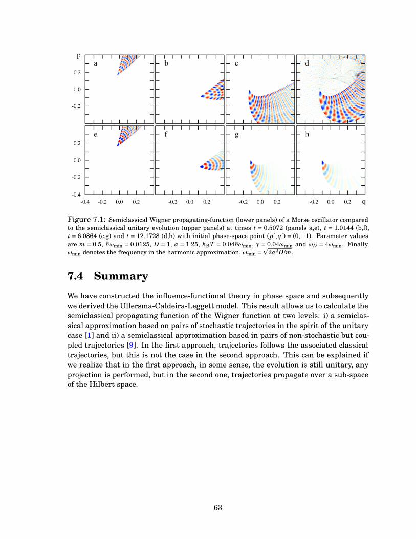
Figure 7.1: Semiclassical Wigner propagating-function (lower panels) of a Morse oscillator comparedto the semiclassical unitary evolution (upper panels) at times t = 0.5072 (panels a,e), t = 1.0144 (b,f),t = 6.0864 (c,g) and t = 12.1728 (d,h) with initial phase-space point (p′, q′) = (0,−1). Parameter valuesare m = 0.5, ~ωmin = 0.0125, D = 1, a = 1.25, kBT = 0.04~ωmin, γ = 0.04ωmin and ωD = 4ωmin. Finally,ωmin denotes the frequency in the harmonic approximation, ωmin =

p2a2D/m.

7.4 Summary

We have constructed the influence-functional theory in phase space and subsequentlywe derived the Ullersma-Caldeira-Leggett model. This result allows us to calculate thesemiclassical propagating function of the Wigner function at two levels: i) a semiclas-sical approximation based on pairs of stochastic trajectories in the spirit of the unitarycase [1] and ii) a semiclassical approximation based in pairs of non-stochastic but cou-pled trajectories [9]. In the first approach, trajectories follows the associated classicaltrajectories, but this is not the case in the second approach. This can be explained ifwe realize that in the first approach, in some sense, the evolution is still unitary, anyprojection is performed, but in the second one, trajectories propagate over a sub-spaceof the Hilbert space.

63

CHAPTER 8

Conclusions and Outlook

In view of the relatively little that is known about semiclassical Wigner propagation,our results provide sufficient qualitative and quantitative evidence to invalidate twopopular connotations: The approach readily captures the time evolution of quantumcoherence effects, including specifically the propagation of Schrödinger cat-states andthe reproduction of tunneling processes. In these cases, it is crucial that even trajectorypairs with large initial separation have to be taken into account. In this respect, onecould consider the application of the semiclassical propagator of the Wigner functionto mixed chaotic systems in molecular dynamics, the study of large complex systemsand introduction of complex trajectories to resolve the caustics and improve the perfor-mance in tunneling processes as tasks for future research.

Additionally, we have provided analytical and numerical evidence that Eq. (5.3)can be interpreted as a global relation between quantum and classical return probabil-ities which can be broken down into contributions of invariant phase-space manifolds.They enter with weight factors that measure the size of the set contributing coher-ently, and lead to important exceptions to Eq. (5.12). Analytical evidence based onpresently available semiclassical approximations [1] indicates they are restricted tothe diagonal r′ = r′′ (where they are least expected) and hence of measure zero. Theyare qualitatively different for integrable systems: In action-angle variables, the size ofthe degenerate sets is independent of time [128] and therefore does not contribute anextra factor t. This in turn reflects the different dimensions and topologies of periodictori vs. isolated unstable periodic orbits, indicating how to generalize this to more in-volved cases like systems with mixed phase space. Merging the different contributionson the classical side into more global quantities like the Frobenius-Perron modes [153],following the route sketched in Sec. 3.4, remains as a challenge for future research.

On the other hand, since at equilibrium, the partition function ZS of a system Swith Hamiltonian H can be calculated in term of the evolution operator in imaginarytime, t =−i~β, i.e. ZS = trU(β) = tr exp(−βH) (cf. [58, 143]), then it is possible to showthat the square of the partition function is given by the trace of the diagonal Wigner

64

propagator,

ZS2 =

∫

df rGW(r,β,r,0). (8.1)

This remark is relevant in the sense that the semiclassical partition function can bereadily calculated form (3.5) and can be understood as the return probability in imagi-nary time. Future research in this direction is also worth considering.

We have also constructed a general semiclassical theory for the dynamics of dissipa-tive systems far from equilibrium with factorizing-initial conditions, which opens thepossibility for a formal and consistent study of the semiclassical spectral statistics ofdissipative systems [75,76], the study of reaction-rate theory far from equilibrium andthe description of decoherent effects in terms of classical manifolds. Moreover, it couldgive some insights about the evolution of entanglement in semiclassical terms [77].

Although, our description of open quantum systems is general enough, the inclu-sion of non-factorizing-initial conditions [140, 154] and more general couplings to thebath [152] could be tasks to do. Additionally, the study of more general models thanCaldeira-Leggett approach such as the unified model for the study of diffusion, localiza-tion and dissipation introduced by Cohen [155,156] for the study of quantal Brownianmotion in dynamical disorder could be treated in the phase-space framework in order togain intuition about the physics behind, mainly because the use of the Wigner functionin this model allowed the distinguishing between two different mechanisms for destruc-tion of coherence: scattering perturbative mechanism and smearing non-perturbativemechanism [157].

Finally, there is a very recent interest in providing a measure for the degree of non-Markovianity of a given physical process [158, 159]. However, the current measureprotocol [158, 159] is based on a average over initial states, i.e., the measure dependson initial states and not directly on dynamical quantities of the system such as thepropagating function, which should be the most natural quantity measuring the degreeof non-Markovianity. The protocol described in [159] could be translate in terms of thepropagating-function as follows: Calculate the propagating function at two differentpoints in phase space ri and r j and calculate the trace distance,

σi, j(t)=∫

df r[

GW(r, t,ri,0)−GW(r, t,r j,0)]

, (8.2)

for Markovian processes this quantity σ(t) should decrease (dσi, j(t)/dt < 0), i.e. infor-mation about the distinguishability flows from the system to the environment while fornon-Markovian processes at certain times this quantity should increase (dσi, j(t)/dt > 0)because information flows form the environment to the system. The next step is trac-ing over initial phase-space points, σ(t) =

∫

di< jσi, j(t) and finally to integrate σ(t) overtime intervals where (dσ(t)/t > 0). This will provide a measure of the non-Markoviancharacter of a physical process.

65

APPENDIX A

Weyl Propagator from Van Vleck Propagator

Van Vleck-Gutzwiller propagator, K (q′′, t′′;q′, t′), [23,24] can be expressed as

K (q′′, t′′;q′, t′)=∑

j

√

1

h f

∣

∣

∣

∣

det(

∂2R j(q′′, t′′;q′, t′)

∂q′′∂q′′

)∣

∣

∣

∣

exp{

1

~R j(q

′′, t′′;q′, t′)− iµ jπ

2

}

, (A.1)

where R j(q′′, t′′;q′, t′) is the Hamilton principal-function. Derivation of the Weyl propa-gator, UW(r) consists of evaluating the Weyl symbol of K (q′′, t′′;q′, t′),

UW(p,q, t)=∫

df uexp(

−i

~p ·u

)

K(

q+u

2, t;q−

u

2,0

)

, (A.2)

by means of stationary-phase approximation [52,86]. Following Berry’s derivation [52],the phase is stationary for

∂

∂u

[

R j

(

q+u

2, t;q−

u

2,0

)

−p ·u]

=∂

∂u

[

∫q−u2

q+u2

dq′′p j(q′′)−H j(r j(r, t))t−p ·u

]

= 1

2p j(0)+ 1

2p j(t)−p= 0.

(A.3)

where we have assumed that the Hamiltonian is time-independent and H j(r j(r, t)) de-notes the energy of the path, which need not be the same as the energy H(r) of thepoint r. Since, by the Weyl symbol transformation q= (q j(0)+q j(t))/2= (q′

j +q′′j )/2 and

by virtue of (A.3), we have that

r=1

2

(

r j(0)+r j(t))

, (A.4)

which defines the midpoint rule: the semiclassical Weyl propagator at t contains con-tribution from the classical paths j that in time t link phase-space points r j(0),r j(t)

66

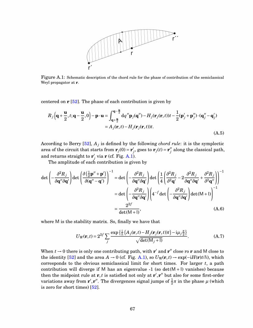
r´

r´´

r

A

Figure A.1: Schematic description of the chord rule for the phase of contribution of the semiclassicalWeyl propagator at r.

centered on r [52]. The phase of each contribution is given by

R j

(

q+ u

2, t;q− u

2,0

)

−p ·u =∫q−u

2

q+u2

dq′′p j(q′′)−H j(r j(r, t))t− 1

2(p′

j +p′′j ) · (q

′′j −q′

j)

= A j(r, t)−H j(r j(r, t))t.(A.5)

According to Berry [52], A j is defined by the following chord rule: it is the symplecticarea of the circuit that starts from r j(0)= r′j, goes to r j(t)= r′′j along the classical path,and returns straight to r′j via r (cf. Fig. A.1).

The amplitude of each contribution is given by

det

(

−∂2R j

∂q′′∂q′

)

det

(

∂(1

2p′′+p′)

∂(q′′−q′)

)−1

= det

(

−∂2R j

∂q′′∂q′

)

det

(

1

4

(

∂2R j

∂2q′ −2∂2R j

∂q′′∂q′ +∂2R j

∂2q′′

))−1

= det

(

−∂2R j

∂q′′∂q′

)(

4−f det

(

−∂2R j

∂q′′∂q′

)

det(M+ I)

)−1

= 22 f

det(M+ I), (A.6)

where M is the stability matrix. So, finally we have that

UW (r, t)= 22 f∑

j

exp{ i~

(

A j(r, t)−H j(r j(r, t))t)

− iµ jπ2

}

√

det(M j + I). (A.7)

When t → 0 there is only one contributing path, with r′ and r′′ close ro r and M close tothe identity [52] and the area A → 0 (cf. Fig. A.1), so UW(r, t) → exp(−iH(r)t/~), whichcorresponds to the obvious semiclassical limit for short times. For larger t, a pathcontribution will diverge if M has an eigenvalue -1 (so det(M+ I) vanishes) becausethen the midpoint rule at r, t is satisfied not only at r′,r′′ but also for some first-ordervariations away from r′,r′′. The divergences signal jumps of 1

2π in the phase µ (whichis zero for short times) [52].

67

APPENDIX B

Split-Operator Method for the Wigner Propagator

The time evolution operator U for a time-independent Hamiltonian H with kineticenergy T = p2/2m and potential energy V = V (q) can be express as the concatenationof N propagators:

U(t, t′)= e−i~

HN∆t = e−i~

(T+V )N∆t =(

e−i~

(T+V )∆t)N

, (B.1)

where ∆t = (t− t′)/N. We separate the kinetic and potential energy terms using theBaker-Campbell-Hausdorff series

e−i~

(V /2+T+V /2)∆t = e−i~

V /2∆te−i~

T∆te−i~

V /2∆teO (∆t3). (B.2)

Although, a non-symmetric decomposition is also possible, the symmetric distributionof V /2, or T/2, cancels all terms of order ∆t2 and makes the approximation accurate upto order ∆t3 [160]. In this way, we have that the evolution operator can be expressedas

U(t, t′)' e−i~

V (q)∆t2 e−

i~

T(p)∆te−i~

V (q)∆t · · · e−i~

V (q)∆te−i~

T(p)∆te−i~

V (q)∆t2 . (B.3)

In order to evaluate (B.3) numerically, we restrict the dimension of the Hilbertspace to be finite, denoted it by DH , sample the position and momentum in intervalsof length L and M, respectively, and store them in vectors of size DH in such way that~ = LM/(2πDH ). On the other hand, since T( p) and V (q) are diagonal in momentumand position representation, respectively, it is convenient to introduce, appropriately,the identities 1=∑

λ |λ⟩⟨λ| and 1=∑

m |m⟩⟨m| in order to obtain a simple representationfor the kinetic-energy and potential energy operators (pλ = Lλ/DH and qm = Mm/DH ).Additionally, we use the fact that ⟨m|λ⟩ = D−1/2

Hexp{2πiλm/DH } and choose as initial

condition the identity matrix (U(t, t) = I). After carrying out this procedure and notic-ing that the choosing of ~ allows the direct implementation of fast Fourier transform

68

routines [92] we can get straightforwardly U(t, t′).To get the Wigner propagator we use expression (2.23)

GW(r′′, t;r′,0)=1

2π~

∫

dq′∫

dq′′exp{

i

~(p′ q′− p′′ q′′)

}

×U∗(

q′′− q′′

2, t; q′− q′

2,0

)

U(

q′′+ q′′

2, t; q′+ q′

2,0

)

,(B.4)

however, since we have restricted the phase space to have finite dimension we have towrite (B.4) in a consistent way. To do that we have to note that here q′, q′′, q′ and q′′

denote integer numbers refereing coordinates of the matrices and take care that thereno exist non-integer indexes for the matrices U and U∗. In order to solve this problemlet us define

UU(q′,q′′; q′, q′′)=

U∗(

q′′− q′′

2 , t; q′− q′

2 ,0)

U(

q′′+ q′′

2 , t; q′+ q′

2 ,0)

q′ and q′′ even,

U∗(

q′′− q′′+12 , t; q′− q′

2 ,0)

U(

q′′+ q′′−12 , t; q′+ q′

2 ,0)

q′ even and q′′ odd,

U∗(

q′′− q′′

2 , t; q′− q′+12 ,0

)

U(

q′′+ q′′

2 , t; q′+ q′−12 ,0

)

q′ odd and q′′ even,

U∗(

q′′− q′′+12 , t; q′− q′+1

2 ,0)

U(

q′′+ q′′−12 , t; q′+ q′−1

2 ,0)

q′ odd and q′′ odd,

and strict the sampling area to −DH

2 + |q′| ≤ q′′

2 < −DH

2 − |q′|. Now we introduce anadditionally quantity ¯UU as

¯UU(q′,q′′; q′, q′′)=

UU(q′, q′′; q′, q′′) q′ and q′′ even,

1π

DH /2−1∑

q′=−DH /2

(−1)q′−q′

q′−q+ 12

UU(q′, q′′; q′, q′′) q′ even and q′′ odd,

1π

DH /2−1∑

q′=−DH /2

(−1)q′−q′

q′−q+ 12

UU(q′, q′′; q′, q′′) q′ odd and q′′ even,

1π2

DH /2−1∑

q′=−DH /2

(−1)q′−q′

q′−q+ 12

DH /2−1∑

q′=−DH /2

(−1)q′−q′

q′−q+ 12

UU(q′, q′′; q′, q′′) q′ odd and q′′ odd.

69

In this way, we can rewrite expression (B.4) finally as

GW(r′′, t;r′,0)= 1

DH

DH /2−1∑

q′=−DH /2

DH /2−1∑

q′′=−DH /2exp

{

2πi(p′ q′− p′′ q′′)/DH

}

¯UU(q′, q′′; q′, q′′).

(B.5)

Since the numerical effort to compute the odd-even and odd-odd combinations ishuge, in a first insight one could restrict the calculation only to the even-even combina-tion. This is equivalent to work with one half of the resolution.

70

APPENDIX C

Numerical Calculation of The Semiclassical Wigner

Propagator

In view of the objective to demonstrate the viability of semiclassical Wigner propaga-tion for numerical applications, we indicate in this appendix how to construct suitablealgorithms for this purpose, without entering into details of their implementation.

C.1 Van Vleck-Based Semiclassical Approximation

The Eqs. (3.5, 3.6) defining the semiclassical Wigner propagator in van Vleck approxi-mation translate into the following straightforward algorithm to compute the propaga-tor as such, not operating on any admissible initial Wigner function:

1. Initial state: Define pairs of initial points r′j± , j = 1, . . ., N, with common midpointr′ = (r′j++r′j−)/2, parameterized, e.g., by spherical coordinates relative to r′. A typ-ical value for the number of classical trajectories, used in most of the calculationsfor one-dimensional systems underlying this work, is N = 106, corresponding to5×105 data points available for the final coarse-graining, step 3b below.

2. Time steps: Realize the integration over time as a sequence of L steps tl−1 →tl, l = 1, . . .,L, tl = t′+ l∆t, ∆t = (t′′− t′)/L. Update the basic ingredients of thepropagator (3.5, 3.6) as follows:

(a) Trajectories r j(tl), j = 1, . . ., N, according to the classical force field,

∆r j(tl)= Jt∇H[r j(tl)]∆t. (C.1)

(b) Stability matrices according to the evolution equation M = MJt∂2H(r)/∂r2

71

(see ,e.g., [161]),

∆M j(tl)=M j(tl)Jt∂

2H(r j(tl))

∂r2j (tl)

∆t. (C.2)

It suggests itself to implement (a) and (b) as a single step, merging Eqs. (C.1,C.2) into a single system of linear equations.

(c) Actions S j as (cf. Fig. 3.1)

∆S j(r′′,r′)= [r j+(tl)−r j−(tl)]∧[∆r j−(tl)+∆r j+(tl)]/2−[H(r j−(tl))−H(r j+(tl))]∆t.

3. Final state:

(a) Separate elliptic from hyperbolic trajectory pairs according to

traj. pair j is

{

ell. det[M j+ −M j−]> 0,

hyp. det[M j+ −M j−]< 0.(C.3)

(b) Within each of the two sheets, coarse-grain the determinantal prefactor|det[M+(t)−M−(t)]|−1/2 and the action S(t) by suitable binning with respectto r′′. In this step, a possibly inhomogeneous distribution of the initial points(as, e.g., for polar coordinates) must be accounted for in terms of weight fac-tors.

(c) Calculate the propagator (3.5) for each sheet and superpose the two contri-butions.

C.2 Propagating Smooth Localized Initial States: To-

wards Monte Carlo Algorithms

For the more common task of propagating well-localized but quantum-mechanicallyadmissible initial states (e.g., Gaussians), the method described in the previous sub-section is not optimal. We can take advantage of the fact that a common midpoint ofall trajectory pairs is not specified, by evaluating all the N(N −1)/2 pairs formed bya set of N classical trajectories to gain a factor O (N) in efficiency. We have to takeinto account, however, that the distribution of centers r jk = (r j + rk)/2 of an ensem-ble of “satellite” phase-space points r j, distributed at random or on an ordered gridwith probability density psat(r), is not this density but its self-convolution, pctr(r) =∫

d2 f r psat(r− r/2)psat(r+ r/2). For Gaussians (4.1) this reduces to a contraction by afactor

p2.

Accordingly, we propose the following scheme for the propagation of smooth local-ized initial states:

1. Initial state: Define a set of initial points r′j, j = 1, . . . , Nsat. A typical value Nsat =1000 now generates Nctr = 5×105 final data points. This can be done in two ways:

72

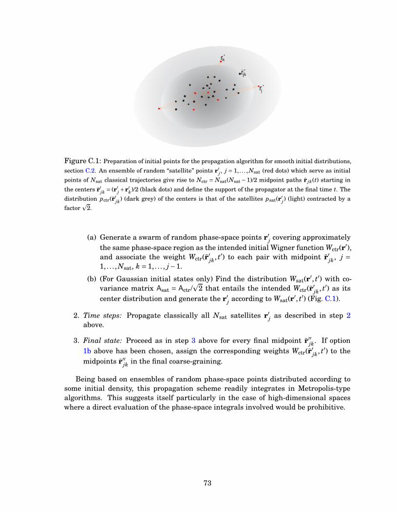
rj

rjk_

rk

Figure C.1: Preparation of initial points for the propagation algorithm for smooth initial distributions,

section C.2. An ensemble of random “satellite” points r′j , j = 1, . . . ,Nsat (red dots) which serve as initial

points of Nsat classical trajectories give rise to Nctr = Nsat(Nsat −1)/2 midpoint paths r jk(t) starting in

the centers r′jk = (r′j +r′k)/2 (black dots) and define the support of the propagator at the final time t. The

distribution pctr(r′jk) (dark grey) of the centers is that of the satellites psat(r′j) (light) contracted by a

factorp

2.

(a) Generate a swarm of random phase-space points r′j covering approximatelythe same phase-space region as the intended initial Wigner function Wctr(r′),and associate the weight Wctr(r′jk, t′) to each pair with midpoint r′jk, j =1, . . ., Nsat, k = 1, . . . , j−1.

(b) (For Gaussian initial states only) Find the distribution Wsat(r′, t′) with co-variance matrix Asat = Actr/

p2 that entails the intended Wctr(r′jk, t′) as its

center distribution and generate the r′j according to Wsat(r′, t′) (Fig. C.1).

2. Time steps: Propagate classically all Nsat satellites r′j as described in step 2above.

3. Final state: Proceed as in step 3 above for every final midpoint r′′jk. If option1b above has been chosen, assign the corresponding weights Wctr(r′jk, t′) to themidpoints r′′jk in the final coarse-graining.

Being based on ensembles of random phase-space points distributed according tosome initial density, this propagation scheme readily integrates in Metropolis-typealgorithms. This suggests itself particularly in the case of high-dimensional spaceswhere a direct evaluation of the phase-space integrals involved would be prohibitive.

73

APPENDIX D

Wigner Propagator Near Periodic Orbits

First, we recall the semiclassical for the Wigner propagator in terms of semiclassicalWeyl propagators given in Sec.3.1 (Eq. (3.2)),

GW (r′′, t;r′,0)=∫

d2 f rexp(

i

~r∧ (r′′−r′)

)

∑

j

(2/h) f

|det(M j + I)|1/2exp

(

i

~A j

(

r′′+r′+ r

2

))

(D.1)

×∑

j′

(2/h) f

|det(M j′ + I)|1/2exp

(

− i

~A j′

(

r′′+r′+ r

2

))

,

choose trajectories j and j′ as periodic orbits only differing from one another by a shiftin time, i.e., r j(T j)= r j(0) and r j(s+T j)= r j(s) and place the origin in rs = rs++rs−

2 . Nowconsider contributions to the r-integral for the propagator from r ≈ ±ds = ±(rs+−rs−)and define r± =±ds +ε. Now let’s choose initial/final r′/r′′ close to the origin,

r′+r′′

2+

r±2

=r′+r′′

2±

ds

2+

ε

2=

r′+r′′+ε

2≈ rs±, (D.2)

r′+r′′

2−

r±2

=r′+r′′

2∓

ds

2−

ε

2=

r′+r′′−ε

2≈ rs∓. (D.3)

Now we apply Berry’s approximation [52] to the Weyl propagator near periodic orbits.i.e., expand phases around ±ds,

A j = S j −r∧M j − I

M j + Ir. (D.4)

74

Now let’s consider the contribution to the propagator near rs from r+

GW (r′′, t;r′)=∫

d2 f ε(2/h)2 f exp

( i~(ds +ε)∧ (r′′−r′)

)

|det(M j + I)|exp

i

~

[

A j

(

r′+r′′+ε

2

)

− A j

(

r′+r′′−ε

2

)]

=(2/h)2 f exp

( i~ds ∧ (r′′−r′)

)

|det(M j + I)|

∫

d2 f εexpi

~

[

ε∧ (r′′−r′)+ A j

(

r′+r′′+ε

2

)

− A j

(

r′+r′′−ε

2

)]

,

now transform to curvilinear coordinates (H, s,r⊥) near rs±

G+W (r′′, t;r′)= (2/h)2 f

|det(M j + I)|exp

(

i

~ds ∧ (r′′−r′)

)∫

dsexp[

− i

~s(H′′−H′)

]

×∫

dH exp[

i

~H(s′′− s′)− H′′+H′+H

2(t−T j)+

H′′+H′−H

2(t+T j)

]

×∫

d2 f−2ε⊥ expi

~

[

ε⊥∧ (r′′−r′)− r′+r′′+ε⊥2

∧M⊥ j − I

M⊥ j + I

r′+r′′+ε⊥2

+r′+r′′−ε⊥2

∧M⊥ j − I

M⊥ j + I

r′+r′′−ε⊥2

]

.

(D.5)

The phase-space integration factorizes into independent integrals over H, s, and ε⊥,respectively. They will be discussed one by one. The H-integration results in deltafunction,

∫

dH exp[

i

~H(s′′− s′)−

H′′+H′+H

2(t−T j)+

H′′+H′−H

2(t+T j)

]

= 2π~δ(s′′−s′−(t−T j)).

Integration over s restricts the propagator to the same energy shell or to the sametorus,

∫

dsexp[

− i

~s(H′′−H′)

]

= 2π~δ(H′′−H′),

while the integral over ε⊥ generates the evolution along the linearized flux in phasespace,

∫

d2 f−2ε⊥ expi

~

[

ε⊥∧ (r′′−r′)−r′+r′′+ε⊥

2∧M⊥ j − I

M⊥ j + I

r′+r′′+ε⊥2

+r′+r′′−ε⊥2

∧M⊥ j − I

M⊥ j + I

r′+r′′−ε⊥2

]

= (2π~)2 f−2

22 f−2|det(M⊥ j + I)|δ

(

r′′−M⊥ jr′)

Combining the contributions from the H−, s-, and ε⊥-integrations,

G+W (r′′, t;r′)= exp

(

i

~ds ∧ (r′′−r′)

)

δ(

H′′−H′) δ∆E(

s′′− s′− (t−T j))

δ(

r′′−M⊥ jr′) .

(D.6)

Similarly, we can calculate the contribution from r−

75

G−W (r′′, t;r′)= exp

(

−i

~ds ∧ (r′′−r′)

)

δ(

H′′−H′) δ∆E(

s′′− s′− (t−T j))

δ(

r′′−M⊥ jr′) .

(D.7)After summing both contributions, the Wigner propagator near a periodic orbit reads,

GW (r′′, t;r′)= 2cos(

1

~ds ∧ (r′′−r′)

)

δ(

H′′−H′) δ∆E(

s′′− s′− (t−T j))

δ(

r′′−M⊥ jr′) .

(D.8)Equation (D.8) exhibits a sufficiently transparent structure to allow for a clear interpre-tation: In the variables with respect to which the Weyl propagator (2.2) is equivalent tothe generic version far off unstable periodic orbits, that is for r⊥ and for s, the Wignerpropagator coincides with the classical Liouville propagator. The factor δ(H′′−H′) isexpected classically from energy conservation [128].

An alternative access to the Wigner propagator near periodic orbits is Berry’s scarfunction, a semiclassical approximation to the Weyl propagator in the energy domain[52]. It responds to the special situation close to a periodic orbit j by using local curvilin-ear coordinates: energy, time, and remaining phase-space directions r j⊥ perpendicularto the orbit. Transformed to the time domain and substituted for the Weyl propagatorin Eq. (2.15), it leads to a semiclassical approximation for the diagonal Wigner propa-gator,

GW j(r, t;r,0)=Tp

j /2π~

|det(M j⊥− I)|δ(r j⊥)δ(t−T j). (D.9)

The primitive period Tpj and the determinantal prefactor measure the length and the

effective cross section, resp., of the “phase-space tube” around the orbit that contributesto the diagonal propagator. By contrast to Eq. (5.21), the degeneracy factor Tp

j appearshere already before tracing: The use of local coordinates condenses the contributionsof periodic points as well as midpoints onto the orbit. Equation (D.9) does not applyoutside the orbit j and therefore does not allow for indiscriminate tracing over all ofphase space.

76

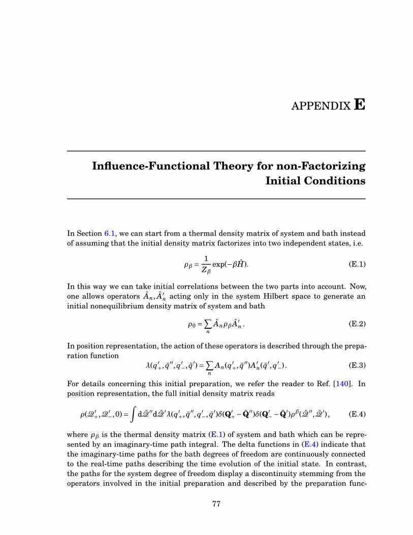
APPENDIX E

Influence-Functional Theory for non-Factorizing

Initial Conditions

In Section 6.1, we can start from a thermal density matrix of system and bath insteadof assuming that the initial density matrix factorizes into two independent states, i.e.

ρβ =1

Zβexp(−βH). (E.1)

In this way we can take initial correlations between the two parts into account. Now,one allows operators An, A′

n acting only in the system Hilbert space to generate aninitial nonequilibrium density matrix of system and bath

ρ0 =∑

nAnρβ A′

n . (E.2)

In position representation, the action of these operators is described through the prepa-ration function

λ(q′+, q′′, q′

−, q′)=∑

nAn(q′

+, q′′)A′n(q′, q′

−) . (E.3)

For details concerning this initial preparation, we refer the reader to Ref. [140]. Inposition representation, the full initial density matrix reads

ρ(Q′+,Q′

−,0)=∫

dQ′′dQ

′λ(q′+, q′′, q′

−, q′)δ(Q′+− Q′′)δ(Q′

−− Q′)ρβ(Q′′,Q′) , (E.4)

where ρβ is the thermal density matrix (E.1) of system and bath which can be repre-sented by an imaginary-time path integral. The delta functions in (E.4) indicate thatthe imaginary-time paths for the bath degrees of freedom are continuously connectedto the real-time paths describing the time evolution of the initial state. In contrast,the paths for the system degree of freedom display a discontinuity stemming from theoperators involved in the initial preparation and described by the preparation func-

77

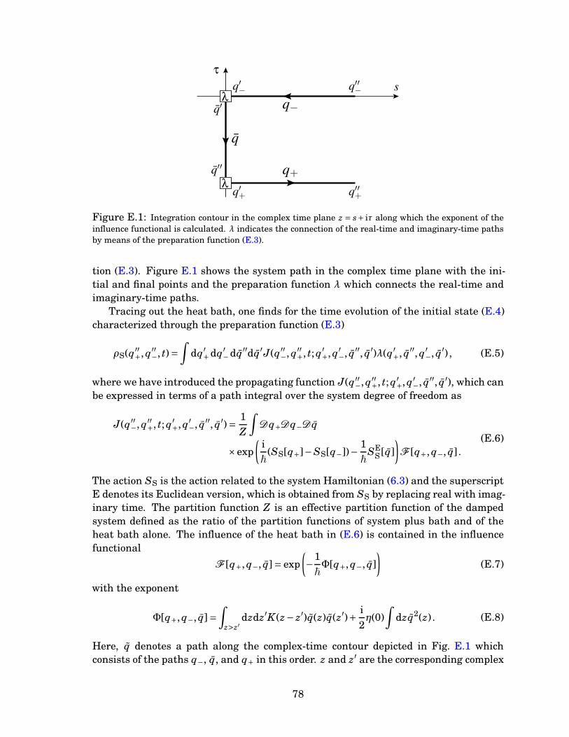
q−

q+

q

s

τ

λ

λ

q′−

q′′−

q′

q′+

q′′+

q′′

Figure E.1: Integration contour in the complex time plane z = s+ iτ along which the exponent of theinfluence functional is calculated. λ indicates the connection of the real-time and imaginary-time pathsby means of the preparation function (E.3).

tion (E.3). Figure E.1 shows the system path in the complex time plane with the ini-tial and final points and the preparation function λ which connects the real-time andimaginary-time paths.

Tracing out the heat bath, one finds for the time evolution of the initial state (E.4)characterized through the preparation function (E.3)

ρS(q′′+, q′′

−, t)=∫

dq′+dq′

−dq′′dq′J(q′′−, q′′

+, t; q′+, q′

−, q′′, q′)λ(q′+, q′′, q′

−, q′) , (E.5)

where we have introduced the propagating function J(q′′−, q′′

+, t; q′+, q′

−, q′′, q′), which canbe expressed in terms of a path integral over the system degree of freedom as

J(q′′−, q′′

+, t; q′+, q′

−, q′′, q′)=1

Z

∫

Dq+Dq−D q

×exp(

i

~(SS[q+]−SS[q−])−

1

~SE

S [q])

F [q+, q−, q] .(E.6)

The action SS is the action related to the system Hamiltonian (6.3) and the superscriptE denotes its Euclidean version, which is obtained from SS by replacing real with imag-inary time. The partition function Z is an effective partition function of the dampedsystem defined as the ratio of the partition functions of system plus bath and of theheat bath alone. The influence of the heat bath in (E.6) is contained in the influencefunctional

F [q+, q−, q]= exp(

−1

~Φ[q+, q−, q]

)

(E.7)

with the exponent

Φ[q+, q−, q]=∫

z>z′dzdz′K (z− z′)q(z)q(z′)+ i

2η(0)

∫

dzq2(z) . (E.8)

Here, q denotes a path along the complex-time contour depicted in Fig. E.1 whichconsists of the paths q−, q, and q+ in this order. z and z′ are the corresponding complex

78

times which satisfy z > z′ along q. The interaction between two points of this path dueto the interaction with the heat bath appears through the noise correlation function(E.11).

As in Sec. 6.1 the microscopic details of the heat bath and its coupling to the sys-tem appear in the reduced system dynamics only through the spectral density of bathoscillators [7,8]

I(ω)=π∞∑

j=1

c2j

2m jω jδ(ω−ω j) . (E.9)

The friction kernel is defined as, η(t)= γ(t)/m

η(t)=2

π

∫∞

0dω

I(ω)

ωcos(ωt) (E.10)

and the correlation function of the noise induced by the coupling to the heat bath isgiven by

αR(z)=∫∞

0

dω

πI(ω)

cosh[ω(12~β− iz)]

sinh(~βω/2), (E.11)

where z is a generally complex time.

E.1 Propagating Function of the Wigner Function

Although this approach can be also expressed in terms of path integrals in phase spacefollowing a similar procedure as in Chap. 7, it is beyond the scope of the present work.However, a similar expression to (6.23) can be derived [9]. Introducing the Wignertransform of the preparation function

λW(p′, q′, p, q)=1

(2π~)2

∫

dq′d ¯qexp[

i

~( p ¯q− p′ q′)

]

λ(q′, q′, ¯q, q) . (E.12)

we obtain for the time evolution of the Wigner function after carrying out the Fouriertransform with respect to q′′

WS(p′′, q′′)=∫

dp′dq′dpdqGW(p′′, q′′, t; p′, q′, p, q)λW(p′, q′, p, q) . (E.13)

By comparison with (E.5) one finds for the relation between the propagating functionintroduced in (E.5) and its Wigner transform

GW(p′′, q′′, t; p′, q′, p, q)= 1

h

∫

dq′′dq′d ¯qexp[

i

~(p′ q′− p′′ q′′− p ¯q)

]

J(q′′, q′′, t; q′, q′, ¯q, q) .

(E.14)For the special case of factorizing initial conditions, the coordinates ¯q, q and the mo-mentum q are to be disregarded and one arrives at the relation (6.23) between thepropagating functions in position and phase space. The presentation of this materialis in order to provide a complete characterization of open quantum systems yet semi-classical analysis and deep analysis are left for further research.

79

APPENDIX F

Ullersma-Caldeira-Leggett Model in Phase Space

With the aim of constructing the Ullersma-Caldeira-Leggett model in phase space wefind more convenient to start with the discrete time-version of the Wigner propagatorof the total system (7.2), i.e.

GW (Rn, n∆t;Rn−1, (n−1)∆t)= 1

(2π~)2(f+F)

∫

d2(f+F)Rn exp

(

−iφn)

, (F.1)

with φn given by (see also Sec. 2.3.2 for more details)

~φn =∆Rn ∧Rn +(

H(

Rn +1

2Rn

)

−H(

Rn −1

2Rn

))

∆t, (F.2)

where R0 =R′, RN =R

′′, ∆Rn =Rn−Rn−1 and Rn = Rn+Rn−12 and H is given by (7.1).

The ingredients for this expression are

∆HB

(

Rn ±1

2Rn

)

=F∑

j=1

P jnP jn

m j+m jω

2jQ jnQ jn (F.3)

∆HSB

(

rn ±1

2rn,Rn ±

1

2Rn

)

=−qn

F∑

j=1c jQ jn − qn

F∑

j=1c jQ jn + qq

F∑

j=1

c2j

m jω2j

. (F.4)

where

∆HB

(

Rn ±1

2Rn

)

= HB

(

Rn +1

2Rn

)

−HB

(

Rn −1

2Rn

)

and

∆HSB

(

rn ±1

2rn,Rn ±

1

2Rn

)

= HSB

(

rn +1

2rn,Rn +

1

2Rn

)

−HSB

(

rn −1

2rn,Rn−

1

2Rn

)

.

80

The symplectic product ∆Rn ∧Rn can be decomposed as

∆Rn ∧Rn =∆rn ∧ rn +F∑

j=1∆R jn ∧ R jn.

Defining

~φS,n =∆rn ∧ rn +(

HS

(

rn +1

2rn

)

−HS

(

rn −1

2rn

))

∆t, (F.5)

we have

GW,n,n−1 =∫

dpn dqn

(2π~)2 exp(

−iφS,n)

F∏

j=1

∫

dF P jn dFQ jn

(2π~)2Fexp

{

−i

~

[

∆P jnQ jn −∆Q jnP jn

+(

P jnP jn

m j+m jω

2jQ jnQ jn − qnc jQ jn − qnc jQ jn + qn qn

c2j

m jω2j

)

∆t

]}

, (F.6)

Integrating over P jn and Q jn we obtain

GW,n,n−1 =∫

dpn dqn

(2π~)2 exp(

−iφS,n)

F∏

j=1δ

(

∆P jn +m jω2j∆tQ jn − qnc j∆t

)

(F.7)

×δ

(

∆Q jn −∆t

m jP jn

)

exp

{

i

~

(

qnc jQ jn − qn qn

c2j

m jω2j

)

∆t

}

,

which can be used to construct the Wigner propagator, GW,N,0, after N-time steps,

GW,N,0 =[

N−1∏

n=1

∫

dpn dqn

][

N∏

n=1

∫

dpn dqn

(2π~)2

]

exp

(

−iN∑

n=1φS,n

)

N−1,F∏

n=1, j=1

∫

dP jndQ jn (F.8)

δ

(

∆Q jn −∆t

m jP jn

)

δ(

∆P jn +m jω2j∆tQ jn − qnc j∆t

)

exp

{

i

~

(

qnc jQ jn − qn qn

c2j

m jω2j

)

∆t

}

.

At this point it is more convenient to introduce the new variables Pn j = ω jPn j andQn j = Qn j/m j and express

Rn, j =Mn, jRn−1, j +Vn, j c j∆t qn (F.9)

where

Mn, j =

4−∆t2ω2j

4+∆t2ω2j

− 4∆tω j

4+∆t2ω2j

4∆tω j

4+∆t2ω2j

4−∆t2ω2j

4+∆t2ω2j

, Vn, j =

4ω j(4+∆t2ω2

j )2∆t

(4+∆t2ω2j )

. (F.10)

We can rewrite the δ-functions in (F.7) as δ(

Rn, j −Mn, jRn−1, j −Vn, j c j∆t qn)

.

81

Integrating over the bath concatenating coordinates, we have

F∏

j=1δ

(

RN, j −N∏

n=1Mn, jR0, j −

N∑

n=0

∏Nk=0Mk, j

∏nk=0Mk, j

Vn, j c j qn∆t

)

. (F.11)

As an example, for N = 3, the factor∏N

n=0Mn, j∏n

k=0Mk, jdenotes the sum

∏3k=0Mk, j

∏nk=0Mk, j

=M3, jM2, jM1, j +M3, jM2, j +M3, j +mathsf 1, (F.12)

where we have considered that M0, j = 1. In the continuous limit, N →∞, we have that

limN→∞

N∏

n=1Mn, j =

(

cosω j t −sinω j tsinω j t cosω j t

)

, (F.13)

limN→∞

N∑

n=0

1∏n

k=0Mk, jVn, j c j qn∆t =

( c j

ω j

∫t0 dt′ cosω j t′q(t′)

− c j

ω j

∫t0 dt′ sinω j t′q(t′)

)

, (F.14)

here we have taken into account that in the continuous limit qn → qn(t). In this way

limN→∞

N∏

k=0Mk, j lim

N→∞

N∑

n=0

1∏n

k=0Mk, jVn, j c j qn∆t =

( c j

ω j

∫t0 dt′ cosω j(t− t′)q(t′)

c j

ω j

∫t0 dt′ sinω j(t− t′)q(t′)

)

. (F.15)

Going back to our initial coordinates Pn j and Qn j the continuous limit of Eq. (F.11)reads

F∏

j=1δ

(

P ′′j −P ′

j cosω j t+m jω jQ′j sinω j t− c j

∫t

0dt′ cosω j(t− t′)q(t′)

)

δ

(

Q′′j −Q′

j cosω j t−P ′

j

m jω jsinω j t−

c j

m jω j

∫t

0dt′sinω j(t− t′)q(t′)

)

, (F.16)

where P j(t)= P ′′j , P j(0) = P ′

j, Q j(t)= Q′′j and Q j(0) =Q′

j. Eq. (F.16) is the propagator ofF non-interacting driven harmonic oscillators, the driving force is c jq(t). Evaluationof the continuous limit presents yet a cumbersome task, the evaluation of the limitN →∞ in the phase of (F.8), omitting all the steps and based on our previous results,we have that

limN→∞

exp

{

i

~

N∑

n=1

(

qnc jQ jn − qn qn

c2j

m jω2j

)

∆t

}

=

exp{

c j

m jω jP ′

j

∫t

0dt′sinω j tq(t)+ c jQ

′j

∫t

0dt′ cosω j tq(t)

+c2

j

m jω j

∫t

0dt′

∫t′

0dt′′ sinω j(t

′− t′′)q(t′′)q(t′)−c2

j

m jω2j

∫t

0dt′q(t′)q(t′)

}

.

(F.17)

82

So, for the Wigner propagator in continuous time we have

GW(r′′,R′′j , t;r′,R′

j,0)=1

(2π~)2

r(t)=r′′∫

r(0)=r′

Dr

r(t)=r′′∫

r(0)=r′

Drexp(

−i

~SS[{r}, {r}, t]

)

×F∏

j=1δ

(

P ′′j −P ′

j cosω j t+ω jQ′j sinω j t− c j

∫t

0dt′ cosω j(t− t′)q(t′)

)

×δ

(

Q′′j −Q′

j cosω j t−P ′

j

m jω jsinω jt−

c j

m jω j

∫t

0dt′ sinω j(t− t′)q(t′)

)

×exp{

i

~

[

c j

m jω jP ′

j

∫t

0dt′ sinω j t

′ q(t′)+ c jQ′j

∫t

0dt′ cosω j t

′ q(t′)

+c2

j

m jω j

∫t

0dt′

∫t′

0dt′′ sinω j(t

′− t′′)q(t′′)q(t′)−c2

j

m jω2j

∫t

0dt′q(t′)q(t′)

]}

,

(F.18)

where

SS[{r}, {r}, t]=∫t

0dt′

[

r∧ r+HS

(

r+ 1

2r

)

−HS

(

r− 1

2r

)]

. (F.19)

Eq. (F.18) is the Wigner propagator of an arbitrary system coupled to a set of F-harmonic oscillators and can be shortly written as

GW(r′′,R′′j , t;r′,R′

j,0)= 1

(2π~)2

r(t)=r′′∫

r(0)=r′

Dr

∫

Drexp(

− i

~SS[{r}, {r}, t]

)

×F∏

j=1δ

(

P ′′j −Pcl

j (P ′j,Q

′j, t)

)

δ(

Q′′j −Qcl

j (P ′j,Q

′j, t)

)

(F.20)

×exp

{

i

~

[

c j

∫t

0dt′Qcl

j (P ′j,Q

′j, t′)q(t′)−

c2j

m jω2j

∫t

0dt′q(t′)q(t′)

]}

,

which allows for a clearer interpretation of each term.

83

Bibliography

[1] T. DITTRICH, C. VIVIESCAS AND L. SANDOVAL. Semiclassical propagator of the Wignerfunction. Phys. Rev. Lett., 96:070403, 2006.

[2] T. DITTRICH, E. A. GÓMEZ AND L. A. PACHÓN. Semiclassical propagation of Wignerfunctions. J. Chem. Phys., 132:214102, 2010.

[3] T. DITTRICH AND L. A. PACHÓN. Cicatrices en el dominio del tiempo y el propagador dela función de Wigner. Rev. Col. Fis., 40:241, 2008.

[4] T. DITTRICH AND L. A. PACHÓN. Time-domain scars: resolving the spectral form factorin phase space. Phys. Rev. Lett., 102:150401, 2009.

[5] R. P. FEYNMAN AND F. L., JR. VERNON. Quantum Brownian motion: The functionalintegral approach. Annals of Physics, 24:118, 1963.

[6] M. S. MARINOV. A new type of phase-space integrals. Phys. Lett. A, 153:5, 1991.

[7] A. O. CALDEIRA AND A. L. LEGGETT. Influence of dissipation on quantum tunneling inmacroscopic systems. Phys. Rev. Lett., 46:211, 1981.

[8] A. O. CALDEIRA AND A. L. LEGGETT. Path integral approach to Brownian motion. Phys-ica A, 121:587, 1983.

[9] L. A. PACHÓN, G.-L. INGOLD AND T. DITTRICH. Nonclassical phase-space trajectoriesfor the damped harmonic quantum oscillator. Chem. Phys., 2010.

[10] F. GALVE, L. A. PACHÓN AND D. ZUECO. Bringing entanglement to the high tempera-ture limit. arXiv.org:1002.1923, 2010.

[11] L. A. PACHÓN, T. DITTRICH AND G.-L. INGOLD. Non-Markovian dissipative semiclassi-cal propagator of the Wigner function. In preparation, 2010.

[12] E. JOOS, H. D. ZEH, C. KIEFER, D. GIULINI, J. KUPSCH, AND I.-O. STAMATESCU.Decoherence and the Appearance of a Classical World in Quantum Theory. Springer,Berlin, 2nd edition, 2003.

84

[13] W. H. ZUREK. Decoherence, einselection, and the quantum origins of the classical. Rev.Mod. Phys., 75:715, 2003.

[14] R. OMNÈS. The Interpretation of Quantum Mechanics. Princeton University Press.,Princeton, New Jersey, 1994.

[15] H. K. ONNES. The resistance of pure mercury at helium temperatures. Commun. Phys.Lab. Univ. Leiden, 12:120, 1911.

[16] M. R. ANDREWS, C. G. TOWNSEND, H.-J. MIESNER, D. S. DURFEE, D. M. KURN AND

W. KETTERLE. Observation of interference between two Bose condensates. Science,275:637, 1997.

[17] K. HORNBERGER, S. GERLICH, H. ULBRICHT, L. HACKERMÜLLER, S. NIMMRICHTER,I. V GOLDT, O. BOLTALINA AND M. ARNDT. Theory and experimental verification ofKapitza-Dirac-Talbot-Lau interferometry. New J. Phys., 11:043032, 2009.

[18] O. ROMERO-ISART, M. L. JUAN, R. QUIDANT AND J. I. CIRAC. Toward quantum super-position of living organisms. New J. Phys., 12:033015, 2010.

[19] G. WENTZEL. Eine verallgemeinerung der quantenbedingungen für die zwecke derwellenmechanik. Zeitschrift der Physik, 38:518, 1926.

[20] H. A. KRAMERS. Wellenmechanik und halbzählige quantisierung. Zeitschrift der Physik,39:828, 1926.

[21] L. BRILLOUIN. La mécanique ondulatoire de Schrödinger: une méthode générale deresolution par approximations successives. Comptes Rendus de l’Academie des Sciences,183:24, 1926.

[22] R. N. P. MAIA, F. NICACIO, R. O. VALLEJOS AND F. TOSCANO. Semiclassical propaga-tion of gaussian wave packets. Phys. Rev. Lett., 100:184102, 2008.

[23] J. H. VAN VLECK. The correspondence principle in the statistical interpretation of quan-tum mechanics. Proc. Natl. Acad. Sci. U.S.A., 14:178, 1928.

[24] M. C. GUTZWILLER. Phase-integral approximation in momentum space and the boundstates of an atom. J. Math. Phys., 8:1979, 1967.

[25] M. C. GUTZWILLER. Periodic orbits and classical quantization conditions. J. Math. Phys.,12:343, 1971.

[26] W. H. MILLER. Quantum mechanical transition state theory and a new semiclassicalmodel for reaction rate constants. J. Chem. Phys., 61:1823, 1974.

[27] P. HÄNGGI, P. TALKNER AND M. BORKOVEC. Reaction-rate theory: fifty years afterKramers. Rev. Mod. Phys., 62:251, 1990.

[28] A. N. KOLMOGOROV. On dynamical systems with an integral invariant on the torus.Dokl. Akad. Nauk SSSR, 93:763, 1953.

[29] A. N. KOLMOGOROV. On conservation of conditionally periodic motions for a smallchange in Hamilton’s functions. Dokl. Akad. Nauk SSSR, 98:527, 1954.

85

[30] V. I. ARNOLD. A proof of the A. N. Kolmogorov’s theorem on the conservation ofconditional-periodic motions in a small change of the Hamilton’s functions. Uspehy Math.Nauk, 18:13, 1963.

[31] J. MOSER. On invariant curves of area-preserving mappings of an annulus. Nachr. Akad.Wiss. Göttingen Math.-Phys. Kl., II:1, 1962.

[32] J. MOSER. Quantum chaology, not quantum chaos. Physica Scripta, 40:335, 1989.

[33] G. CASATI, B. V. CHIRIKOV, J. FORD AND F. M. IZNELEV. True quantum chaos? aninstructive example. In G. Casati and J. Ford, editors, Stochastic behavior in classicaland quantum systems, volume 93 of Lecture Notes in Physics, page 334. Springer-Verlag,Berlin/Heidelberg, 1979.

[34] M. V. BERRY. Semiclassical mechanics of regular and irregular motion. In H G. Iooss,R. H. G. Helleman, and R. Stora, editors, Chaotic behaviour of deterministic systems,volume XXXVI of Les Houches Lectures, page 171. North-Holland, Amsterdam, 1983.

[35] M. V. BERRY. Regular and irregular semiclassical wave functions. J. Phys. A, 10:2083,1977.

[36] H. J. KORSCH AND M. V. BERRY. Evolution of Wigner’s phase-space density under anon-integrable quantum map. Physica, 3D:627, 1981.

[37] B. V. CHIRIKOV, F. M. IZRACLCV, AND D. L. SHEPELYANSKY. Dynamical stochasticityin classical and quantum mechanics. Sov. Sci. Rev., C3:209, 1981.

[38] M. C. GUTZWILLER. Phase-integral approximation in momentum space and the boundstates of an atom. II. J. Math. Phys., 10:1004, 1969.

[39] M. C. GUTZWILLER. Energy spectrum according to classical mechanics. J. Math. Phys.,11:1791, 1970.

[40] R. BALIAN AND C. BLOCH. Distribution of eigenfrequencies for the wave equation in afinite domain : I. Three-dimensional problem with smooth boundary surface. Ann. Phys.(N.Y.), 60:401, 1970.

[41] R. BALIAN AND C. BLOCH. Distribution of eigenfrequencies for the wave equation in afinite domain : II. Electromagnetic field. Riemannian spaces. Ann. Phys. (N.Y.), 64:371,1971.

[42] R. BALIAN AND C. BLOCH. Distribution of eigenfrequencies for the wave equation in afinite domain : III. Eigenfrequency density oscillations. Ann. Phys. (N.Y.), 69:76, 1972.

[43] R. BALIAN AND C. BLOCH. Solution of the Schrödinger equation in terms of classicalpaths. Ann. Phys. (N.Y.), 85:514, 1972.

[44] M. V. BERRY AND M. TABOR. Closed orbits and the regular bound spectrum. Proc. R.Soc. A, 349:101, 1976.

[45] M. V. BERRY AND M. TABOR. Level clustering in the regular spectrum. Proc. R. Soc. A,356:375, 1977.

86

[46] M. V. BERRY AND M. TABOR. Calculating the bound spectrum by path summation inaction-angle variables. J. Phys. A: Math. Gen., 10:371, 1977.

[47] A. I. SCHNIRELMAN. Ergodic properties of eigenfunctions. Uspehy Math. Nauk, 29:181,1974.

[48] M. V. BERRY. Semi-classical mechanics in phase space: a study of Wigner’s function.Phil. Trans. R. Soc. A., 287:237, 1977.

[49] A. VOROS. Semi-classical ergodicity of quantum eigenstates in the Wigner repre-sentation. In G. Casati and J. Ford, editors, Stochastic behavior in classical andquantum systems, volume 93 of Lecture Notes in Physics, page 326. Springer-Verlag,Berlin/Heidelberg, 1979.

[50] E. J. HELLER. Bound-state eigenfunctions of classically chaotic Hamiltonian systems:Scars of periodic orbits. Phys. Rev. Lett., 53:1515, 1984.

[51] E. J. HELLER. Qualitative properties of eigenfunctions of classically chaotic Hamiltoniansystems. In T-H. Seligman and H. Nishioka, editors, Quantum Chaos and StatisticalNuclear Physics, volume 263 of Lectures Notes in Physics, page 162. Springer, BerlinHeidelberg, 1986.

[52] M. V. BERRY. Quantum scars of classical closed orbits in phase space. Proc. Roy. Soc.Lond. A, 423:219, 1989.

[53] F. TOSCANO, M. A. M. DE AGUIAR AND A. M. OZORIO DE ALMEIDA. Scars of the Wignerfunction. Phys. Rev. Lett., 86:59, 2001.

[54] R. GAMBINI. The measurement problem and the reduction postulate of quantum me-chanics. arXiv.org:quant-ph/9803025, 1998.

[55] L. D. LANDAU AND I. M. LIFSHITZ. Quantum Mechanics (Nonrelativistic Theory). Perg-amon, Oxford, 1965.

[56] A. EINSTEIN, B. PODOLSKY AND N. ROSEN. Can quantum-mechanical description ofphysical reality be considered complete? Phys. Rev., 47:777, 1935.

[57] P. P. DE M. RIOS AND A. M. OZORIO DE ALMEIDA. On the propagation of semiclassicalWigner functions. J. Phys. A, 35:2609, 2002.

[58] U. WEISS. Quantum Dissipative Systems. World Scientific, Singapore, 2nd edition, 1993.

[59] C.-I. UM, K.-H. YEON AND T. F. GEORGE. The quantum damped harmonic oscillator.Phys. Rep., 362:63, 2002.

[60] P. ULLERSMA. An exactly solvable model for Brownian motion. I. derivation of theLangevin equation. Physica, 32:27, 1966.

[61] P. ULLERSMA. An exactly solvable model for Brownian motion. II. derivation of theFokker–Planck equation and the master equation. Physica, 32:56, 1966.

[62] P. ULLERSMA. An exactly solvable model for Brownian motion. III. motion of a heavymass in a linear chain. Physica, 32:74, 1966.

87

[63] F. GROSSMANN. A semiclassical approach to dissipation in quantum mechanics. J. Chem.Phys., 103:3696, 1995.

[64] W. T. STRUNZ. Path integral, semiclassical and stochastic propagators for Markovianopen systems. J. Phys. A: Math. Gen., 30:4053, 1997.

[65] A. M. OZORIO DE ALMEIDA. Decoherence of semiclassical Wigner functions. J. Phys. A:Math. Gen., 36:67, 2002.

[66] O. BRODIER AND A. M. OZORIO DE ALMEIDA. Symplectic evolution of Wigner functionsin Markovian open systems. Phys. Rev. E, 69:016204, 2004.

[67] W. KOCH, F. GROSSMANN, J. T. STOCKBURGER AND J. ANKERHOLD. Non-Markoviandissipative semiclassical dynamics. Phys. Rev. Lett., 100:230402, 2008.

[68] H. APPEL AND M. DI VENTRA. Stochastic quantum molecular dynamics. Phys. Rev. B,80:212303, 2009.

[69] H. DAMMAK, Y. CHALOPIN, M. LAROCHE, M. HAYOUN, AND J.-J. GREFFET. Quantumthermal bath for molecular dynamics simulation. Phys. Rev. Lett., 103:190601, 2009.

[70] J. L. ALONSO, A. CASTRO, P. ECHENIQUE, V. POLO, A. RUBIO, D. ZUECO. Ab initiomolecular dynamics on the electronic boltzmann equilibrium distribution. arXiv.org:cond-mat:1002.4899, 2010.

[71] A. M. OZORIO DE ALMEIDA, P. DE M. RIOS AND O. BRODIER. Semiclassical evolutionof dissipative Markovian systems. J. Phys. A: Math. Theor., 42:065306, 2009.

[72] O. BRODIER AND A. M. OZORIO DE ALMEIDA. Complex WKB evolution of Markovianopen systems. arXiv.org:0906.4288, 2009.

[73] G. LINDBLAD. On the generators of quantum dynamical semigroups. Commun. MathPhys, 48:119, 1976.

[74] V. GORINI, A. FRIGERIO, M. VERRI, A. KOSSAKOWSKI AND E. C. G. SUDARSHAN. Prop-erties of quantum markovian master equations. Rep. Math. Phys., 13:149, 1978.

[75] D. BRAUN. Spectral properties of dissipative chaotic quantum maps. Chaos, 9:730, 1999.

[76] D. BRAUN, P. A. BRAUN AND F. HAAKE. Semiclassics for a dissipative quantum map.Physica D, 131:265, 1999.

[77] A. M. OZORIO DE ALMEIDA. Entanglement in phase space. In A. Buchleitner, C. Vivi-escas, and M. Tiersch, editors, Entanglement and Decoherence, volume 768 of LectureNotes in Physics, page 157. Springer-Verlag, Berlin/Heidelberg, 2009.

[78] G. S. ENGEL, T. R. CALHOUN, E. L. READ, T.-K. AHN, T. MANCAL, Y.-C. CHENG,R. E. BLANKENSHIP AND G. R. FLEMING. Evidence for wavelike energy transferthrough quantum coherence in photosynthetic systems. Nature, 446:782, 2007.

[79] E. Collini, C. Y. Wong, K. E. Wilk, P. M. G. Curmi, P. Brumer, and G. D. Scholes. Co-herently wired light-harvesting in photosynthetic marine algae at ambient temperature.Nature, 463:644, 2010.

88

[80] W. H. MILLER. Quantum dynamics of complex molecular systems. Proc. Natl. Acad. Sci.U.S.A., 102:6660, 2005.

[81] L. M. K. VANDERSYPEN, M. STEFFEN, G. BREYTA, C. S. YANNON, M. H. SHERWOOD

AND I. L. CHUANG. Experimental realization of Shor’s quantum factoring algorithmusing nuclear magnetic resonance. Nature, 414:883, 2001.

[82] K.-K. Ni, S. Ospelkaus, D. Wang, G. Quéméner, B. Neyenhuis, M. H. G. de Miranda, J. L.Bohn, J. Ye, and D. S. Jin. Dipolar collisions of polar molecules in the quantum regime.Nature, 464:1324, 2010.

[83] M. HILLERY, R. F. O’CONNELL, M. O. SCULLY AND E. P. WIGNER. Distribution func-tions in physics: Fundamentals. Phys. Rep., 106:121, 1984.

[84] E. P. WIGNER. On the quantum correction for thermodynamic equilibrium. Phys. Rev.,40:749, 1932.

[85] M.-J. GIANNONI, A. VOROS AND J. ZINN-JUSTIN (EDS.). Chaos and Quantum Physics,Les Houches Lectures LII. North-Holland-Elsevier, Amsterdam, 1992.

[86] A. M. OZORIO DE ALMEIDA. The Weyl representation in classical and quantum mechan-ics. Phys. Rep., 295:265, 1998.

[87] L. E. REICHL. A modern course in statistical physics. Wiley-Interscience, New York,1998.

[88] D. MUSTARD. The fractional Fourier transform and the Wigner distribution. J. Austral.Math. Soc. Ser. B, 38:209, 1996.

[89] J. E. MOYAL. Quantum mechanics as a statistical theory. Proc. Camb. Phil. Soc., 45:99,1949.

[90] J. MOIX, E. POLLAK AND J. SHAO. Generalized Liouville time-dependent perturbationtheory. Phys. Rev. A, 80:052103, 2009.

[91] M. S. MARINOV AND B. SEGEV. Quantum tunneling in the Wigner representation. Phys.Rev. A, 54:4752, 1996.

[92] W. H. PRESS, S. A. TEUKOLSKY, W. T. VETTERLING AND B. P. FLANNERY. Numeri-cal Recipes in Fortran: The Art of Scientific Computing. Cambridge University Press.,Cambridge, United Kingdom, 1992.

[93] R. P. FEYNMAN AND A. R. HIBBS. Quantum physics and path integrals. McGraw–Hill,New York, 1965.

[94] A. ARGÜELLES AND T. DITTRICH. Wigner function for discrete phase space: Exorcisingghost images. Physica A, 356:72, 2005.

[95] O. AGAM AND N. BRENNER. Semiclassical Wigner functions of quantum maps on a torus.J. Phys. A: Math. Gen., 28:1345, 1995.

[96] A. ARGÜELLES. Construcción de la función de Wigner para espacio de fase discretos.Master’s thesis, Universidad Nacional de Colombia, Bogotá, Colombia, December 2004.

89

[97] D. A. MONRROY. Función de Wigner en espacio de fase discreto y tomografía cuántica.Bachelor’s thesis, Universidad Nacional de Colombia, Bogotá, Colombia, December 2010.

[98] H. P. HSU. Fourier Analysis. Simon & Schuster, New York, 1970.

[99] M. S. MARINOV. Path integrals in quantum theory: an outlook of basic concepts. Phys.Rep., 60:1, 1980.

[100] N. L. BALAZS. Weyl’s association, Wigner’s function and affine geometry. Physica A,102:236, 1980.

[101] W. H. ZUREK. Sub-Planck structure in phase space and its relevance for quantum deco-herence. Nature, 412:712, 2001.

[102] E. J. HELLER. Wigner phase space method: Analysis for semiclassical applications. J.Chem. Phys., 65:1289, 1976.

[103] C. JAFFÉ AND P. BRUMER. Classical Liouville mechanics and intramolecular relaxationdynamics. J. Phys. Chem., 88:4829, 1984.

[104] C. JAFFÉ AND P. BRUMER. Classical analog of pure-state quantum dynamics. Phys. Rev.Lett., 54:8, 1985.

[105] C. JAFFÉ AND P. BRUMER. Classical-quantum correspondence in the distribution dy-namics of integrable systems. J. Chem. Phys., 82:2330, 1985.

[106] J. WILKIE AND P. BRUMER. Quantum-classical correspondence via Liouville dynamics.I. Integrable systems and the chaotic spectral decomposition. Phys. Rev. A, 55:27, 1997.

[107] J. WILKIE AND P. BRUMER. Quantum-classical correspondence via Liouville dynamics.II. Correspondence for chaotic Hamiltonian systems. Phys. Rev. A, 55:43, 1997.

[108] R. L. HUDSON. When is the Wigner quasi-probability density non-negative?Rep. Math. Phys., 6:249, 1974.

[109] E. J. HELLER. Wavepacket dynamics and quantum chaology. In M.-J. Giannoni, A. Voros,and J. Zinn-Justin, editors, Chaos and Quantum Physics, volume LII of Les HouchesLectures, page 547. North-Holland, Amsterdam, 1991.

[110] W. P. SCHLEICH. Quantum Optics in Phase Space. Wiley–VCH, Berlin, 2001.

[111] P. M. MORSE. Diatomic molecules according to the wave mechanics. II. Vibrational levels.Phys. Rev., 34:57, 1929.

[112] J. P. DAHL AND M. SPRINGBORG. The Morse oscillator in position space, momentumspace, and phase space. J. Chem. Phys., 88:4535, 1988.

[113] M. A. SEPÚLVEDA AND F. GROSSMANN. Time-dependent semiclassical mechanics. Adv.Chem. Phys., 96:191, 1996.

[114] F. GROSSMANN. A hierarchy of semiclassical approximations based on Gaussianwavepackets. Comments At. Mol. Phys., 34:141, 1999.

[115] C. HARABATI AND J. M. ROST AND F. GROSSMANN. Long-time and unitary propertiesof semiclassical initial value representations. J. Chem. Phys., 120:26, 2004.

90

[116] A. KENFACK AND J. M. ROST AND A. M. OZORIO DE ALMEIDA. Optimal representationsof quantum states by Gaussians in phase space. J. Phys. B: At. Mol. Opt. Phys., 37:1645,2004.

[117] M. V. BERRY AND K. E. MOUNT. Semiclassical approximations in wave mechanics. Rep.Prog. Phys., 35:315, 1972.

[118] S. C. CREAGH. Tunnelling in multidimensional systems. J. Phys. A: Math. Gen., 27:4969,1994.

[119] A. L. XAVIER JR. AND M. A. M. DE AGUIAR. Phase-space approach to the tunnel effect:A new semiclassical traversal time. Phys. Rev. Lett, 79:3323, 1997.

[120] N. L. BALAZS AND A. VOROS. Wigner’s function and tunneling. Ann. Phys. (N. Y.),199:123, 1990.

[121] M. NOVAES. Real trajectories in the semiclassical coherent state propagator. J. Math.Phys, 46:102102, 2005.

[122] M. S. MARINOV AND B. SEGEV. Barrier penetration by wave packets and the tunnelingtimes. Phys. Rev. A, 55:3580, 1997.

[123] F. GROSSMANN, T. DITTRICH, P. JUNG, AND P. HÄNGGI . Coherent destruction of tun-neling. Phys. Rev. Lett., 67:516, 1991.

[124] M. SIEBER AND K. RICHTER. Correlations between periodic orbits and their rôle inspectral statistics. Physica Scripta, T90:128, 2001.

[125] O. BOHIGAS, M. J. GIANNONI, AND C. SCHMIT . Characterization of chaotic quantumspectra and universality of level fluctuation laws. Phys. Rev. Lett., 54:1, 1984.

[126] F. HAAKE. Quantum Signatures of Chaos, 2nd edition. Springer, Berlin, 2000.

[127] H. J. STÖCKMANN. Quantum Chaos: an introduction. Cambridge University Press,Cambridge, 1999.

[128] T. DITTRICH. Spectral statistics for 1-D disordered systems: a semiclassical approach.Phys. Rep., 271:267, 1996.

[129] J. H. HANNAY AND A. M. OZORIO DE ALMEIDA. Periodic orbits and a correlation func-tion for the semiclassical density of states. J. Phys. A: Math. Gen., 17:3429, 1984.

[130] S. MÜLLER, S. HEUSLER, P. BRAUN, F. HAAKE AND A. ALTLAND. Semiclassical foun-dation of universality in quantum chaos. Phys. Rev. Lett., 93:014103, 2004.

[131] T. DITTRICH AND U. SMILANSKY. Spectral properties of systems with dynamical local-ization. I. the local spectrum. Nonlinearity, 4:59, 1991.

[132] T. DITTRICH AND U. SMILANSKY. Spectral properties of systems with dynamical local-ization. II. finite sample approach. Nonlinearity, 4:85, 1991.

[133] M. SARACENO. Classical structures in the quantized baker transformation.Ann. Phys. (NY), 199:37, 1990.

91

[134] F. MCLAFFERTY. On classical paths and the Wigner path integral. J. Chem. Phys.,78:3253, 1983.

[135] J. H. HANNAY AND M. V. BERRY. Quantization of linear maps on a torus - Fresneldiffraction by a periodic grating. Physica, 1D:267, 1980.

[136] N. L. BALAZS AND A. VOROS. The quantized Baker’s transformation. Ann. Phys. (N.Y.),190:1, 1989.

[137] A. M. OZORIO DE ALMEIDA AND M. SARACENO. Periodic orbit theory for the quantizedbaker’s map. Ann. Phys., 210:1, 1991.

[138] M. SARACENO AND A. VOROS. Boundary contributions to the semiclassical traces of theBaker’s map. Physica D, 6:206, 1994.

[139] M. SARACENO AND R. O. VALLEJOS. The quantized D-transformation. Chaos, 6:193,1996.

[140] H. GRABERT, P. SCHRAMM AND G.-L. INGOLD. Quantum Brownian motion: The func-tional integral approach. Phys. Rep., 168:115, 1988.

[141] V. HAKIM, V. AMBEGAOKAR. Quantum theory of a free particle interacting with a lin-early dissipative environment. Phys. Rev. A, 32:423, 1985.

[142] C. ZERBE AND P. HÄNGGI. Brownian parametric quantum harmonic oscillator withdissipation. Phys. Rev. E, 52:1533, 1995.

[143] G.-L. INGOLD. Path integrals and their application to dissipative quantum systems. InA. Buchleitner and K. Hornberger, editors, Coherent Evolution in Noisy Environments,volume 611 of Lecture Notes in Physics, page 1. Springer Verlag, Berlin-Heidelberg-NewYork, 2002.

[144] P. HÄNGGI. Generalized Langevin equations: A useful tool for the perplexed modeller ofnonequilibrium fluctuations? In L. Schimansky-Geier and T. Pöschel, editors, StochasticDynamics, volume 484 of Lecture Notes in Physics, page 15. Springer Verlag, Berlin,Heidelberg, 1997.

[145] J. ANDREASEN, H. CAO, A. TAFLOVE, P. KUMAR AND C.-QI CAO. Finite-differencetime-domain simulation of thermal noise in open cavities. Phys. Rev. A, 77:023810, 2008.

[146] N. WAX, ED. Selected papers on noise and stochastic processes. Dover, New York, 1954.

[147] J. T. STOCKBURGER AND H. GRABERT. Non-Markovian quantum state diffusion. Chem.Phys., 268:249, 2001.

[148] J. T. STOCKBURGER AND H. GRABERT. Exact c-number representation of non-Markovian quantum dissipation. Phys. Rev. Lett., 88:170407, 2002.

[149] H. M. WISEMAN AND J. M. GAMBETTA. Pure-state quantum trajectories for generalnon-Markovian systems do not exist. Phys. Rev. Lett., 101:140401, 2008.

[150] V. B. MAGALINSKII. Dynamical model in the theory of the Brownian motion. Zh. Eksp.Teor. Fiz., 36:1942, 1959.

92

[151] H. KOHLER AND F. SOLS. Quasiclassical frustration. Phys. Rev. B, 72:180404, 2005.

[152] H. KOHLER AND F. SOLS. Dissipative quantum oscillator with two competing heat baths.New J. Phys., 8:149, 2006.

[153] A. V. ANDREEV, O. AGAM, B. D. SIMONS AND B. L. ALTSHULER . Quantum chaos,irreversible classical dynamics, and random matrix theory. Phys. Rev. Lett., 76:3947,1996.

[154] C. M. SMITH AND A. O. CALDEIRA. Generalized Feynman-Vernon approach to dissipa-tive quantum systems. Phys. Rev. A, 36:3509, 1987.

[155] D. COHEN. Unified model for the study of diffusion localization and dissipation. Phys.Rev. E, 55:1422, 1997.

[156] D. COHEN. Quantum dissipation versus classical dissipation for generalized Brownianmotion. Phys. Rev. Lett., 78:2878, 1997.

[157] D. COHEN. Quantal Brownian motion-dephasing and dissipation. J. Phys. A, 31:8199,1998.

[158] H.-P. BREUER, E.-M. LAINE AND J. PIILO. Measure for the degree of non-Markovianbehavior of quantum processes in open systems. Phys. Rev. Lett., 103:210401, 2009.

[159] E.-M. LAINE, J. PIILO AND H.-P. BREUER. Measure for the non-Markovianity of quan-tum processes. Phys. Rev. A, 81:062115, 2010.

[160] M. D FEIT, J. A. FLECK JR. AND A. STEIGER. Solution of the Schrödinger equation bya spectral method. J. Comput. Phys., 47:412, 1982.

[161] F. GROSSMANN. A semiclassical hybrid approach to many particle quantum dynamics.J. Chem. Phys., 125:014111, 2006.

93