Embed Size (px)
Citation preview

Cohabitation vs marriage: Marriage matching with peereffects
Ismael Mourifie and Aloysius Siow
University of Toronto
December 2014, Penn State

Motivation
Trends on US marital behavior since the seventies:The marriage rate has decreased.
The cohabitation rate has increased.
The unmatched rate has increased.
Some evidence on increased positive assortative matching in marriage byeducation (PAM).
Increases in earnings inequality, PAM and married women labor supplyled to increases in family earnings inequality. (Burtless (1999);Greenwood, Jeremy, Nezih Guner, Georgi Kocharkov, and Cezar Santos(2014); Carbone and Cahn (2014)).
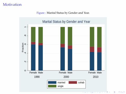
Motivation
Figure : Marital Status by Gender and Year.
0.2
.4.6
.81
Fra
ctio
n
1990 2000 2010
Female Male Female Male Female Male
Marital Status by Gender and Year
married cohabsingle

Motivation
Researchers have investigated different causes for these changesincluding
Changes in reproductive technologies.
Changes in access to reproductive technologies.
Changes in family laws.
Changes in earnings inequality and changes in welfare regimes.
E.g. Burtless 1999; Choo Siow 2006a; Fernandez, Guner and Knowles 2005;Fernandez-Villaverde, et. al. 2014; Goldin and Katz 2002; Greenwood, et. al.(2012, 2014) etc...
Most of this research ignored changes in population supplies over time.Often, they also ignore peer effects in marital behavior.
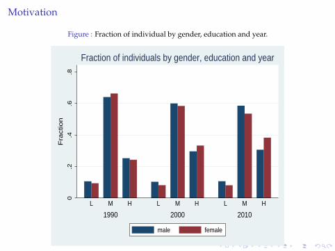
Motivation
Figure : Fraction of individual by gender, education and year.
0.2
.4.6
.8
1990 2000 2010
L M H L M H L M H
Fra
ctio
nFraction of individuals by gender, education and year
male female
Motivation
This change in the sex ratio may have exacerbated the decline in themarriage rate.
It may also potentially changed marriage matching patterns.
Peer effects may have also affected cohabitation and other maritalbehavior. E.g. Waite, et. al. 2000; Fernandez-Villaverde, et. al. (2014))
Adamopoulou (2012) shows that there are positive peer effects on themarital decisions of young adults.

Main objective
The objective of this paper is to first provide an elementary marriagematching function (MMF),
which can be used to parameterize different causes of changes in maritalbehavior.
while allowing for peer effects and changes in population supplies.
Second, we estimate the changes in the parameters of the MMF whichcapture the evolution of marital behavior in the US between 1990 and2010

What we do
We propose a new static empirical marriage matching function (MMF):the Cobb Douglas MMF
The Cobb Douglas MMF encompasses:Choo-Siow frictionless transferable utility MMF (CS)
The CS with frictional transfers.
The Dagsvik Menziel non-transferable utility MMF.
The Chiappori, Salanie and Weiss MMF (CSW).
The marriage matching with peer effects (CSPE).
Properties of this Cobb Douglas MMF are presented.
Existence and uniqueness proof of the marriage distribution areprovided.
Comparative statistics are derived.

What we do(1)
Identification and estimation are presented.
Empirical ApplicationThe CD MMF is estimated on US marriage and cohabitation data by statesfrom 1990 to 2010.
CS with peer effects is not rejected.
There are peer and scale effects in the US marriage markets.
Positive assortative matching in marriage and cohabitation by educationalattainment are relatively stable from 1990 to 2010.
The CS Benchmark
Consider a society with I, i = 1, .., I, types of men and J, j = 1, .. J, typesof women.
Let m and f be the population vectors of men and women respectively.
Let θ be a vector of parameters.
A marriage matching function (MMF) is an I× J matrix valued functionµ(m, f ; θ) whose typical element is µij, the number type i men married totype j women.
The CS Benchmark(1)
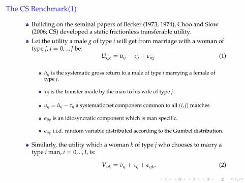
Building on the seminal papers of Becker (1973, 1974), Choo and Siow(2006; CS) developed a static frictionless transferable utility.
Let the utility a male g of type i will get from marriage with a woman oftype j, j = 0, .., J be:
Uijg = uij − τij + εijg (1)
uij is the systematic gross return to a male of type i marrying a female oftype j.
τij is the transfer made by the man to his wife of type j.
uij = uij − τij a systematic net component common to all (i, j) matches
εijg is an idiosyncratic component which is man specific.
εijg i.i.d. random variable distributed according to the Gumbel distribution.
Similarly, the utility which a woman k of type j who chooses to marry atype i man, i = 0, .., I, is:
Vijk = vij + τij + εijk. (2)
The CS Benchmark(2)
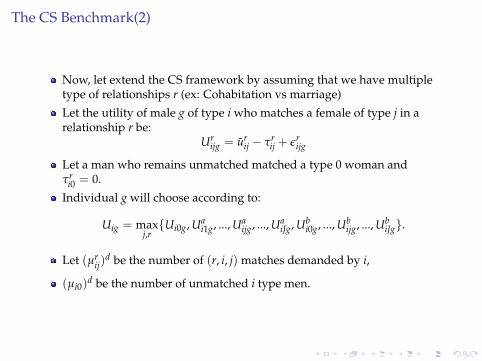
Now, let extend the CS framework by assuming that we have multipletype of relationships r (ex: Cohabitation vs marriage)
Let the utility of male g of type i who matches a female of type j in arelationship r be:
Urijg = ur
ij − τrij + εr
ijg
Let a man who remains unmatched matched a type 0 woman andτr
i0 = 0.
Individual g will choose according to:
Uig = maxj,r{Ui0g, Ua
i1g, ..., Uaijg, ..., Ua
iJg, Ubi0g, ..., Ub
ijg, ..., UbiJg}.
Let (µrij)
d be the number of (r, i, j) matches demanded by i,
(µi0)d be the number of unmatched i type men.

The CS Benchmark(3)
Following the well known McFadden result, we have:
(µrij)
d
mi= P(Ur
ijg −Ur′ikg ≥ 0, k = 1, ..., J; r′ = a, b),
where mi denotes the number of men of type i.From above, we obtain a quasi-demand equation by type i men for(r, i, j) relationships.
ln(µr
ij)d
(µi0)d = urij − ui0 − τr
ij, (3)

The CS Benchmark(4)
The quasi-supply equation of type j women for (r, i, j) relationships isgiven by:
ln(µr
ij)s
(µ0j)s = vrij − v0j + τr
ij. (4)
The matching market clears when, given equilibrium transfers τrij, we
have for all (r, i, j):(µr
ij)d = (µr
ij)s = µr
ij. (5)
Substituting (5) into equations (3) and (4) we get the following MMF:
lnµr
ij√
µi0µ0j= πr
ij ∀ (r, i, j) (6)
where πrij = ur
ij − ui0 + vrij − v0j. (called the the gains to marriage)
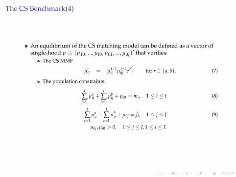
The CS Benchmark(4)
An equilibrium of the CS matching model can be defined as a vector ofsingle-hood µ ≡ (µ10, ..., µI0, µ01, ..., µ0J)
′ that verifies:The CS MMF.
µrij = µ1/2
i0 µ1/20j eπr
ij for r ∈ {a, b}. (7)
The population constraints.
J
∑j=1
µaij +
J
∑j=1
µbij + µi0 = mi, 1 ≤ i ≤ I (8)
I
∑i=1
µaij +
I
∑i=1
µbij + µ0j = fj, 1 ≤ j ≤ J (9)
µ0j, µi0 > 0, 1 ≤ j ≤ J, 1 ≤ i ≤ I.

The CS Benchmark(5)
In others terms, an equilibrium of the CS matching model is the solutionof the following quadratic system of equations:
J
∑j=1
βiβI+j(eπa
ij + eπbij ) + β2
i = mi, 1 ≤ i ≤ I
I
∑i=1
βiβI+j(eπa
ij + eπbij ) + β2
I+j = fj, 1 ≤ j ≤ J
βi, βI+j > 0, 1 ≤ j ≤ J, 1 ≤ i ≤ I.
where βi =√
µi0 and βI+j =√
µ0j

The CS Benchmark(6)
Using a variational approach Decker et al (2013) showed that for anyadmissible (m, f ; θ), µ exists and is unique.
Galichon and Salanie (2013) showed also the existence and theuniqueness using an alternative approach.
Properties of the CS MMF
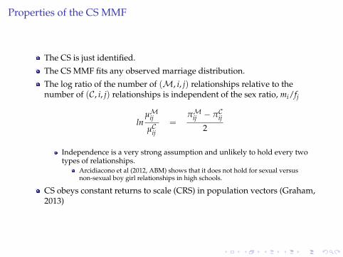
The CS is just identified.
The CS MMF fits any observed marriage distribution.
The log ratio of the number of (M, i, j) relationships relative to thenumber of (C, i, j) relationships is independent of the sex ratio, mi/fj
lnµMij
µCij=
πMij − πCij2
Independence is a very strong assumption and unlikely to hold every twotypes of relationships.
Arcidiacono et al (2012, ABM) shows that it does not hold for sexual versusnon-sexual boy girl relationships in high schools.
CS obeys constant returns to scale (CRS) in population vectors (Graham,2013)
Survey on the related literatureWe can distinguish two main directions in the subsequent literature to the CSMMF.
1 One branch relaxes the specification of the idiosyncratic component εrijg.
The net systematic gains from matching, urij = ur
ij − τrij and vr
ij = vrij − τr
ij,from CS is retained.
The transfer is still used to clear the marriage market.
Chiappori, Salanie and Wiess (2012; CSW) allows the variance of εrijg to differ
by gender and type and obtains
lnµr
ij
(µi0)1−λij (µ0j)
λij=
πrij
σi + Σj∀ (r, i, j) (10)
where λij =Σj
σi+Σj.
Graham (2013) provides a wide set of comparative statistics for a specialcase of CSW i.e. λij = λ.
Galichon and Salanie (2012, GS) further generalizes the distributions ofidiosyncratic utilities.
Chiappori and Salanie (2014) provides an excellent state of the art survey ofthe above and related models.
2 The second branch studies other behavioral specifications for the netsystematic return from marriage, ur
ij and vrij
Survey on the related literature (1)
We can distinguish two main directions in the subsequent literature to the CSMMF.
1 One branch relaxes the specification of the idiosyncratic component εrijg.
2 The second branch studies other behavioral specifications for the netsystematic return from marriage, ur
ij and vrij
Dagsvik (2000) assumes that transfers are not available to clear the marriagemarket i.e. τr
ij = 0
He assumes that the idiosyncratic payoff of man g of type i marryingwoman k of type j, εr
ijgk, is distributed i.i.d. Gumbel.
He uses the deferred acceptance algorithm to solve for a matchingequilibrium and obtain the following non-transferable utility MMF for largemarriage markets:
lnµr
ij
µi0µ0j= πij ∀ (r, i, j) (11)
Menziel (2012) shows that (11) obtains under less restrictive assumptionsabout the distribution of εr
ijgk. Call (11) the DM MMF.
Survey on the related literature (2)
We can distinguish two main directions in the subsequent literature to the CSMMF.
1 One branch relaxes the specification of the idiosyncratic component εrijg.
2 The second branch studies other behavioral specifications for the netsystematic return from marriage, ur
ij and vrij
The DM MMF also fits any observed marriage distribution.
Unlike CS, it obeys increasing return to scale in population vectors.
When there is more than one type of relationship, the log odds of thenumbers of different types of relationships is independent of the sexratio, for all the model surveyed i.e. The CS, CSW and DM MMF.
Choo-Siow with peer effect (CSPE)
Let the utility of male g of type i who matches a female of type j in arelationship r be:
Urijg = ur
ij + φri ln µr
ij − τrij + εr
ijg, where (12)
urij + φr
i ln µrij: Systematic gross return to a male of type i matching to a
female of type j in relationship r.
φri : Coefficient of peer effect for relationship r, 1 ≥ φr
i ≥ 0.
µrij: Equilibrium number of (r, i, j) relationships.
ui0 + φ0i ln µ0
i0 is the systematic payoff that type i men get from remainingunmatched, 1 ≥ φ0
i ≥ 0.
The above empirical model for multinomial choice with peer effects isstandard. See Brock and Durlauf (2001)
What is new is our application to two sided matching.
Choo-Siow with peer effect (CSPE)
Male’s utilityUr
ijg = urij + φr
i ln µrij − τr
ij + εrijg
We allow the peer effect to differ by relationship.
There is no apriori reason to rank φ0i versus φr
i .
For example, unmarried individuals spend more time with their unmarriedfriends than married individuals with their married friends.
On the other hand, married individuals may want to live in communiteswith couples like themselves so that local firms will provide services to them(E.g. Compton and Pollak (2007); Costa and Kahn (2000)).
CSPE
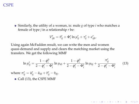
Similarly, the utility of a woman, is: male g of type i who matches afemale of type j in a relationship r be:
Vrijk = vr
ij + Φri ln µr
ij + τrij + εr
ijk,
Using again McFadden result, we can write the men and womenquasi-demand and supply and clears the matching market using thetransfers. We get the following MMF
ln µrij =
1− φ0i
2− φri −Φr
iln µi0 +
1− φ0i
2− φri −Φr
iln µ0j +
πrij
2− φri −Φr
i(13)
where πrij = ur
ij − ui0 + vrij − v0j.
Call (13), the CSPE MMF

Some results on the CSPE
When there is no peer effect or all the peer effect coefficients are thesame (homogeneous peer effects),
φ0i = Φ0
j = φri = Φr
j
we recover the CS MMF
No peer effect, or homogenous peer effects, generates observationallyequivalent MMFs.
If we cannot reject CS using marriage matching data alone, we alsocannot reject homogenous peer effects.
This lack of identification is our version of the reflection problem inManski’s linear-in-mean peer effects mode.
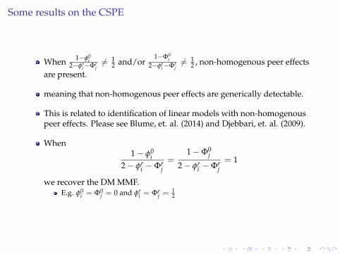
Some results on the CSPE
When 1−φ0i
2−φri−Φr
j6= 1
2 and/or1−Φ0
j2−φr
i−Φrj6= 1
2 , non-homogenous peer effectsare present.
meaning that non-homogenous peer effects are generically detectable.
This is related to identification of linear models with non-homogenouspeer effects. Please see Blume, et. al. (2014) and Djebbari, et. al. (2009).
When1− φ0
i2− φr
i −Φrj=
1−Φ0j
2− φri −Φr
j= 1
we recover the DM MMF.E.g. φ0
i = Φ0j = 0 and φr
i = Φrj =
12
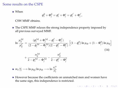
Some results on the CSPE
Whenφ0
i + Φ0j = φr
i + Φrj = φr′
i + Φr′j ,
CSW MMF obtains.
The CSPE MMF relaxes the strong independence property imposed byall previous surveyed MMF.
lnµMij
µCij=
(φMi + ΦMj − φCi −ΦCj )
(2− φMi −ΦMj )(2− φCi −ΦCj )
[(1− φ0
i ) ln µi0 + (1−Φ0j ) ln µ0j
](14)
+πMij
2− φMi −ΦMj−
πCij
2− φCi −ΦCj
mi/fj −→ ln µ0j; ln µi0 −→ lnµMijµCij
However because the coefficients on unmatched men and women havethe same sign, this independence is restricted.
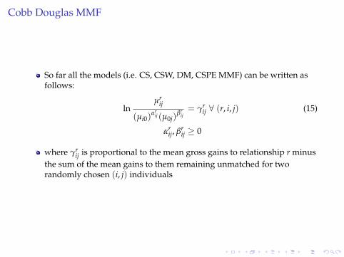
Cobb Douglas MMF
So far all the models (i.e. CS, CSW, DM, CSPE MMF) can be written asfollows:
lnµr
ij
(µi0)αr
ij (µ0j)βr
ij= γr
ij ∀ (r, i, j) (15)
αrij, βr
ij ≥ 0
where γrij is proportional to the mean gross gains to relationship r minus
the sum of the mean gains to them remaining unmatched for tworandomly chosen (i, j) individuals
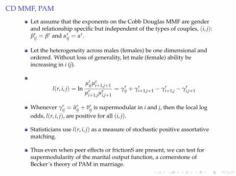
CD MMF, PAM
Let assume that the exponents on the Cobb Douglas MMF are genderand relationship specific but independent of the types of couples, (i, j):βr
ij = βr and αrij = αr.
Let the heterogeneity across males (females) be one dimensional andordered. Without loss of generality, let male (female) ability beincreasing in i (j).
l(r, i, j) = lnµr
ijµri+1,j+1
µri+1,jµ
ri,j+1
= γrij + γr
i+1,j+1 − γri+1,j − γr
i,j+1
Whenever γrij = ur
ij + vrij is supermodular in i and j, then the local log
odds, l(r, i, j), are positive for all (i, j).
Statisticians use l(r, i, j) as a measure of stochastic positive assortativematching.
Thus even when peer effects or frictionS are present, we can test forsupermodularity of the marital output function, a cornerstone ofBecker’s theory of PAM in marriage.
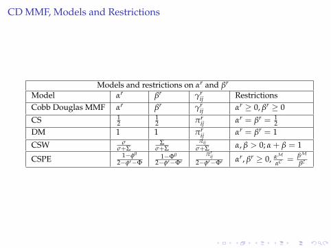
CD MMF, Models and Restrictions
Models and restrictions on αr and βr
Model αr βr γrij Restrictions
Cobb Douglas MMF αr βr γrij αr ≥ 0, βr ≥ 0
CS 12
12 πr
ij αr = βr = 12
DM 1 1 πrij αr = βr = 1
CSW σσ+Σ
Σσ+Σ
πijσ+Σ α, β > 0; α + β = 1
CSPE 1−φ0
2−φr−Φ1−Φ0
2−φr−Φrπr
ij2−φr−Φr αr, βr ≥ 0, αM
αC=
βM
βC
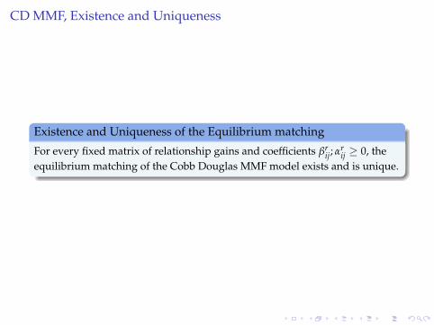
CD MMF, Existence and Uniqueness
Existence and Uniqueness of the Equilibrium matching
For every fixed matrix of relationship gains and coefficients βrij; αr
ij ≥ 0, theequilibrium matching of the Cobb Douglas MMF model exists and is unique.

CD MMF, Existence and Uniqueness’s proof
As shown previously, an equilibrium of the Cobb Douglas MMF is thesolution of the following system of equations:
mi = µi0 +J
∑j=1
µαMiji0 µ
βMij0j eγMij +
J
∑j=1
µαCiji0 µ
βCij0j eγCij , for 1 ≤ i ≤ I, (16)
fj = µ0j +I
∑i=1
µαMiji0 µ
βMij0j eγMij +
I
∑i=1
µαCiji0 µ
βCij0j eγCij , for 1 ≤ j ≤ J. (17)
Could we write this system as a F.O.C of a variational problem? It seemsnot true in general.
The method of GS cannot be directly applied due to the presence of thepeer effect.
CD MMF, Existence and Uniqueness’s proof
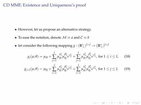
However, let us propose an alternative strategy.
To ease the notation, denoteM≡ a and C ≡ b
let consider the following mapping g : (R∗+)I+J → (R∗+)
I+J
gi(µ; θ) = µi0 +J
∑j=1
µαa
iji0 µ
βaij
0j eγaij +
J
∑j=1
µαb
iji0 µ
βbij
0j eγbij , for 1 ≤ i ≤ I, (18)
gj+I(µ; θ) = µ0j +I
∑i=1
µαa
iji0 µ
βaij
0j eγaij +
I
∑i=1
µαb
iji0 µ
βbij
0j eγbij , for 1 ≤ j ≤ J. (19)
CD MMF, Existence and Uniqueness’s proof
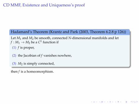
Hadamard’s Theorem (Krantz and Park (2003, Theorem 6.2.8 p 126))
Let M1 and M2 be smooth, connected N-dimensional manifolds and letf : M1 → M2 be a C1 function if
(1) f is proper,
(2) the Jacobian of f vanishes nowhere,
(3) M2 is simply connected,
then f is a homeomorphism.
CD MMF, Existence and Uniqueness’s proof
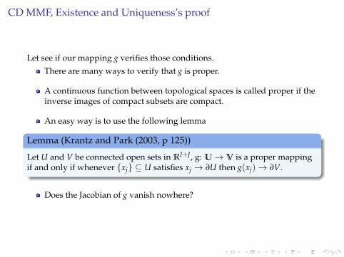
Let see if our mapping g verifies those conditions.
There are many ways to verify that g is proper.
A continuous function between topological spaces is called proper if theinverse images of compact subsets are compact.
An easy way is to use the following lemma
Lemma (Krantz and Park (2003, p 125))
Let U and V be connected open sets in RI+J, g: U→ V is a proper mappingif and only if whenever {xj} ⊆ U satisfies xj → ∂U then g(xj)→ ∂V.
Does the Jacobian of g vanish nowhere?

CD MMF, Existence and Uniqueness’s proof
Let write
µαr
iji0 µ
βrij
0j eγrij = eαr
ijlnµi0+βrijlnµ0j+γr
ij ,
≡ eδrij .
Let Jg(µ) be the Jacobian of g.
After a simple derivation we can show that Jg(µ) takes the followingform:
Jg(µ) =
((Jg)11(µ) (Jg)12(µ)(Jg)21(µ) (Jg)22(µ)
)with
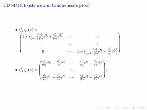
CD MMF, Existence and Uniqueness’s proof
(Jg)11(µ) =1 + ∑J
j=1
[αa
1jµ10
eδa1j +
αb1j
µ10eδb
1j]· · · 0
.... . .
...
0 · · · 1 + ∑Jj=1
[αa
IjµI0
eδaIj +
αbIj
µI0eδb
Ij]
(Jg)21(µ) =
αa
11µ10
eδa11 +
αb11
µ10eδb
11 · · · αaI1
µI0eδa
I1 +αb
I1µI0
eδbI1
.... . .
...αa
1Jµ10
eδa1J +
αb1J
µ10eδb
1J · · · αaIJ
µI0eδa
IJ +αb
IJµI0
eδbIJ
,
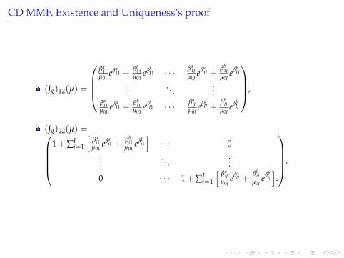
CD MMF, Existence and Uniqueness’s proof
(Jg)12(µ) =
βa
11µ01
eδa11 +
βb11
µ01eδb
11 · · · βa1J
µ0Jeδa
1J +βb
1Jµ0J
eδb1J
.... . .
...βa
I1µ01
eδaI1 +
βbI1
µ01eδb
I1 · · · βaIJ
µ0Jeδa
IJ +βb
IJµ0J
eδbIJ
,
(Jg)22(µ) =1 + ∑I
i=1
[βa
i1µ01
eδai1 +
βbi1
µ01eδb
i1
]· · · 0
.... . .
...
0 · · · 1 + ∑Ii=1
[βa
iJµ0J
eδaiJ +
βbiJ
µ0Jeδb
iJ
].
.

CD MMF, Existence and Uniqueness’s proof
Let us denote every element of Jg(µ), Jk,l with 1 ≤ k, l ≤ I + J.
We can remark that |Jll| > ∑I+Jk 6=l |Jkl| for l = 1, ..., I + J.
So , Jg(µ) is a column diagonally dominant matrix or diagonallydominant in the sense of McKenzie (1960) far all µ > 0.
Thus, Jg(µ), for all µ > 0, is a non-singular matrix. (Proof see McKenzie(1960).
Then, our mapping g is an homeomorphism.
Therefore, the system of equation (18) admits a unique solution.
We can easily check that the solution is economically relevant in thesense that 0 < µeq < (m′, f ′)′.
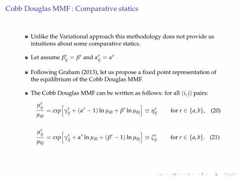
Cobb Douglas MMF : Comparative statics
Unlike the Variational approach this methodology does not provide usintuitions about some comparative statics.
Let assume βrij = βr and αr
ij = αr
Following Graham (2013), let us propose a fixed point representation ofthe equilibrium of the Cobb Douglas MMF.
The Cobb Douglas MMF can be written as follows: for all (i, j) pairs:
µrij
µi0= exp
[γr
ij + (αr − 1) ln µi0 + βr ln µ0j
]≡ ηr
ij for r ∈ {a, b}, (20)
µrij
µ0j= exp
[γr
ij + αr ln µi0 + (βr − 1) ln µ0j
]≡ ζr
ij for r ∈ {a, b}. (21)
Cobb Douglas MMF : Comparative statics (1)
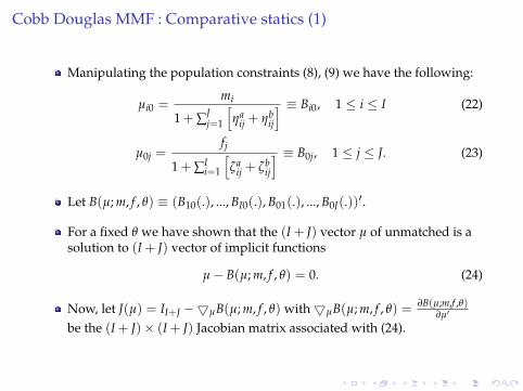
Manipulating the population constraints (8), (9) we have the following:
µi0 =mi
1 + ∑Jj=1
[ηa
ij + ηbij
] ≡ Bi0, 1 ≤ i ≤ I (22)
µ0j =fj
1 + ∑Ii=1
[ζa
ij + ζbij
] ≡ B0j, 1 ≤ j ≤ J. (23)
Let B(µ; m, f , θ) ≡ (B10(.), ..., BI0(.), B01(.), ..., B0J(.))′.
For a fixed θ we have shown that the (I + J) vector µ of unmatched is asolution to (I + J) vector of implicit functions
µ− B(µ; m, f , θ) = 0. (24)
Now, let J(µ) = II+J −5µB(µ; m, f , θ) with5µB(µ; m, f , θ) =∂B(µ;m,f ,θ)
∂µ′
be the (I + J)× (I + J) Jacobian matrix associated with (24).
Cobb Douglas MMF : Comparative statics (2)
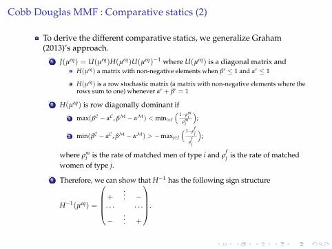
To derive the different comparative statics, we generalize Graham(2013)’s approach.
1 J(µeq) = U(µeq)H(µeq)U(µeq)−1 where U(µeq) is a diagonal matrix andH(µeq) a matrix with non-negative elements when βr ≤ 1 and αr ≤ 1
H(µeq) is a row stochastic matrix (a matrix with non-negative elements where therows sum to one) whenever αr + βr = 1
2 H(µeq) is row diagonally dominant if
1 max(βC − αC , βM − αM) < mini∈I
( 1−ρmi
ρmi
);
2 min(βC − αC , βM − αM) > −maxj∈J
( 1−ρfj
ρfj
);
where ρmi is the rate of matched men of type i and ρ
fj is the rate of matched
women of type j.
3 Therefore, we can show that H−1 has the following sign structure
H−1(µeq) =
+... −
. . . . . .
−... +
.
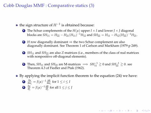
Cobb Douglas MMF : Comparative statics (3)
the sign structure of H−1 is obtained because:1 The Schur complements of the H(µ) upper I× I and lower J× J diagonal
blocks are SH11 = H22 −H21(H11)−1H12 and SH22 = H11 −H12(H22)
−1H21.
2 H row diagonally dominant⇒ the two Schur complement are alsodiagonally dominant. See Theorem 1 of Carlson and Markham (1979 p 249).
3 SH11 and SH22 are also Z-matrices (i.e., members of the class of real matriceswith nonpositive off-diagonal elements).
4 Then, SH11 and SH22 are M-matrices =⇒ SH−111 = 0 and SH−1
22 = 0. seeTheorem 4.3 of Fiedler and Ptak (1962).
By applying the implicit function theorem to the equation (24) we have:1 ∂µ
∂mi= J(µ)−1 ∂B
∂mifor 1 ≤ i ≤ I
2 ∂µ∂fj
= J(µ)−1 ∂B∂fj
for all 1 ≤ j ≤ J

Cobb Douglas MMF : Comparative statics (4)
Comparative Statics (1)
Let µ be the equilibrium matching distribution of the Cobb Douglas MMFmodel. If the coefficients βr and αr respect the restrictions
1 0 < βr; αr ≤ 1 for r ∈ {M, C};2 max(βC − αC , βM − αM) < mini∈I
(1−ρm
iρm
i
);
3 min(βC − αC , βM − αM) > −maxj∈J
( 1−ρfj
ρfj
);
Type-specific elasticities of unmatched.
miµk0
∂µk0∂mi≥
1
m∗imkm∗k
∑Jj=1
[αMµMkj +αCµCkj][βMµMkj +βCµCkj]
f ∗j> 0 if k 6= i
mim∗i
[1 + 1m∗i
∑Jj=1
[αMµMij +αCµCij ][βMµMij +βCµCij ]
f ∗j] > 1 if k = i,
1 ≤ k ≤ I.
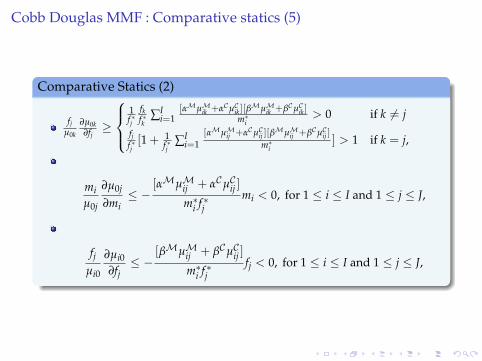
Cobb Douglas MMF : Comparative statics (5)
Comparative Statics (2)
fjµ0k
∂µ0k∂fj≥
1f ∗j
fkf ∗k
∑Ii=1
[αMµMik +αCµCik ][βMµMik +βCµCik ]
m∗i> 0 if k 6= j
fjf ∗j[1 + 1
f ∗j∑I
i=1[αMµMij +αCµCij ][β
MµMij +βCµCij ]
m∗i] > 1 if k = j,
miµ0j
∂µ0j
∂mi≤ −
[αMµMij + αCµCij ]
m∗i f ∗jmi < 0, for 1 ≤ i ≤ I and 1 ≤ j ≤ J,
fjµi0
∂µi0∂fj≤ −
[βMµMij + βCµCij ]
m∗i f ∗jfj < 0, for 1 ≤ i ≤ I and 1 ≤ j ≤ J,
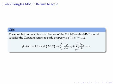
Cobb Douglas MMF : Return to scale
CRSThe equilibrium matching distribution of the Cobb Douglas MMF modelsatisfies the Constant return to scale property if βr + αr = 1 i.e.
βr + αr = 1 for r ∈ {M, C} ⇒I
∑i=1
∂µ
∂mimi +
J
∑j=1
∂µ
∂fjfj = µ.
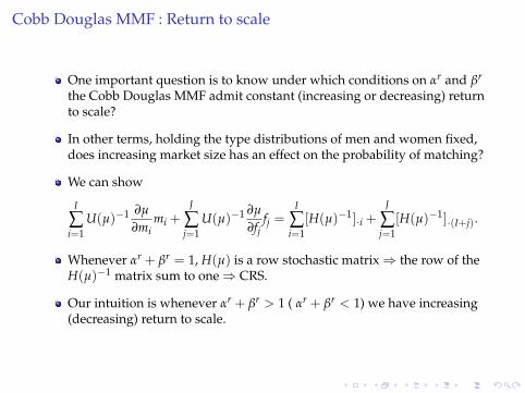
Cobb Douglas MMF : Return to scale
One important question is to know under which conditions on αr and βr
the Cobb Douglas MMF admit constant (increasing or decreasing) returnto scale?
In other terms, holding the type distributions of men and women fixed,does increasing market size has an effect on the probability of matching?
We can show
I
∑i=1
U(µ)−1 ∂µ
∂mimi +
J
∑j=1
U(µ)−1 ∂µ
∂fjfj =
I
∑i=1
[H(µ)−1]·i +J
∑j=1
[H(µ)−1]·(I+j).
Whenever αr + βr = 1, H(µ) is a row stochastic matrix⇒ the row of theH(µ)−1 matrix sum to one⇒ CRS.
Our intuition is whenever αr + βr > 1 ( αr + βr < 1) we have increasing(decreasing) return to scale.
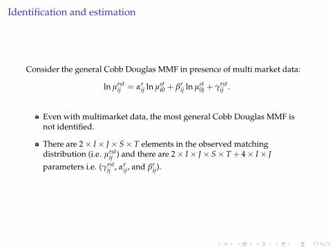
Identification and estimation
Consider the general Cobb Douglas MMF in presence of multi market data:
ln µrstij = αr
ij ln µsti0 + βr
ij ln µst0j + γrst
ij .
Even with multimarket data, the most general Cobb Douglas MMF isnot identified.
There are 2× I× J× S× T elements in the observed matchingdistribution (i.e. µrst
ij ) and there are 2× I× J× S× T + 4× I× Jparameters i.e. (γrst
ij , αrij, and βr
ij).
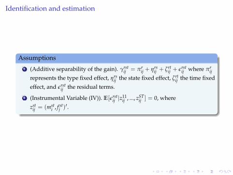
Identification and estimation
Assumptions
1 (Additive separability of the gain). γrstij = πr
ij + ηrsij + ζrt
ij + εrstij where πr
ijrepresents the type fixed effect, ηrs
ij the state fixed effect, ζrtij the time fixed
effect, and εrstij the residual terms.
2 (Instrumental Variable (IV)). E[εrstij |z
11ij , ..., zST
ij ] = 0, where
zstij = (mst
i , f stj )′.
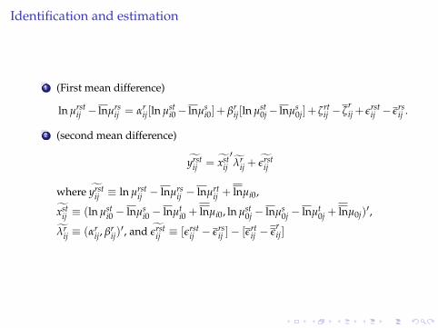
Identification and estimation
1 (First mean difference)
ln µrstij − lnµrs
ij = αrij[ln µst
i0− lnµsi0]+ βr
ij[ln µst0j− lnµs
0j]+ ζrtij − ζ
rij + εrst
ij − εrsij .
2 (second mean difference)
yrstij = xst
ij′λr
ij + εrstij
where yrstij ≡ ln µrst
ij − lnµrsij − lnµrt
ij + lnµi0,
xstij ≡ (ln µst
i0 − lnµsi0 − lnµt
i0 + lnµi0, ln µst0j − lnµs
0j − lnµt0j + lnµ0j)
′,
λrij ≡ (αr
ij, βrij)′, and εrst
ij ≡ [εrstij − εrs
ij ]− [εrtij − ε
rij]
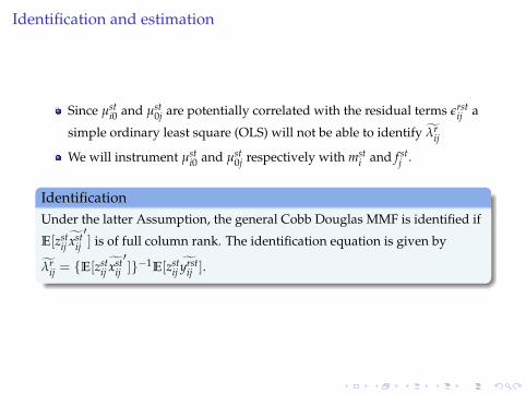
Identification and estimation
Since µsti0 and µst
0j are potentially correlated with the residual terms εrstij a
simple ordinary least square (OLS) will not be able to identify λrij
We will instrument µsti0 and µst
0j respectively with msti and f st
j .
IdentificationUnder the latter Assumption, the general Cobb Douglas MMF is identified if
E[zstij xst
ij′] is of full column rank. The identification equation is given by
λrij = {E[zst
ij xstij′]}−1E[zst
ij yrstij ].

Empirical Application
We study the marriage matching behavior of 26-30 years old women and28-32 years old men with each other in the US for 1990, 2000 and 2010.
The 1990 and 2000 data is from the 5% US census.
The 2010 data is from aggregating three years of the 1% AmericanCommunity Survey from 2008-2010.
A state year is considered as an isolated marriage market.
There were 51 states which includes DC.
Individuals are distinguished by their schooling level: less than highschool (L), high school graduate (M) and university graduate (H).
A cohabitating couple is one where a respondent answered that they arethe “unmarried partner” of the head of the household.
Empirical Application
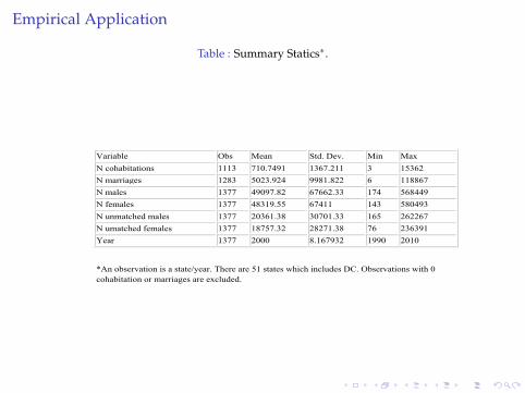
Table : Summary Statics∗.
Variable Obs Mean Std. Dev. Min Max N cohabitations 1113 710.7491 1367.211 3 15362 N marriages 1283 5023.924 9981.822 6 118867 N males 1377 49097.82 67662.33 174 568449 N females 1377 48319.55 67411 143 580493 N unmatched males 1377 20361.38 30701.33 165 262267 N umatched females 1377 18757.32 28271.38 76 236391 Year 1377 2000 8.167932 1990 2010
*An observation is a state/year. There are 51 states which includes DC. Observations with 0 cohabitation or marriages are excluded.
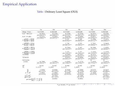
Empirical Application
Table : Ordinary Least Square (OLS).
1a 1b 2a 2b 3a 3b
Dep. Var. LCOH LMAR LCOH LMAR LCOH LMAR LU_M (𝛼) 0.562 0.536 0.320 0.244 0.557 0.626 (0.041)** (0.048)** (0.075)** (0.061)** (0.084)** (0.056)** LU_F (β) 0.531 0.665 0.630 0.609 0.827 0.939 (0.040)** (0.047)** (0.076)** (0.058)** (0.078)** (0.051)**
𝐿𝐻𝐻 ∗𝑀𝑀𝐻𝑀 ∗𝑀𝐻 2.31
(0.078)**
2.44 (0.069)**
2.290 (0.071)**
2.412 (0.048)**
𝐿𝑀𝑀 ∗ 𝐿𝐿𝐿𝑀 ∗𝑀𝐿 1.78
(0.087)**
2.52 (0.082)**
1.781 (0.080)**
2.464 (0.063)**
𝐿𝐻𝑀 ∗𝑀𝐿𝑀𝑀 ∗ 𝐻𝐿 0.784
(0.147)**
1.43 (0.092)**
0.796 (0.145)**
1.426 (0.084)**
𝐿𝑀𝐻 ∗ 𝐿𝑀𝑀𝑀 ∗ 𝐿𝐻 1.33
(0.141)** 1.37
(0.101)** 1.344
(0.135)** 1.379
(0.083)** Y2000 0.289 -0.287 0.313 -0.277 (0.042)** (0.032)** (0.037)** (0.022)** Y2010 0.627 -0.604 0.615 -0.667 (0.041)** (0.037)** (0.040)** (0.030)** STATE Y Y _cons -4.788 -3.981 -2.842 1.172 -7.359 -5.015 (0.383)** (0.441)** (0.196)** (0.158)** (0.772)** (0.543)** R2 0.51 0.45 0.90 0.95 0.92 0.97 N 1,113 1,283 1,113 1,283 1,113 1,283
𝛼𝛽 1.058
(0.137) 0.806
(0.115) 0.508
(0.178) 0.400
(0.138) 0.673
(0.146) 0.667
(0.082) 𝛼 + 𝛽 1.093
(0.039) 1.202
(0.045) 0.950
(0.018) 0.853
(0.016) 1.384
(0.079) 1.57
(0.057) 𝛼ℳ
𝛽ℳ𝛽𝒞
𝛼𝒞
0.762 (0.147)
0.788 (0.387)
0.991 (0.246)
𝑝𝑟𝑜𝑏 𝛼ℳ = 𝛼𝒞
𝛽ℳ = 𝛽𝒞
0.091 0.001 0.117
* p<0.05; ** p<0.01
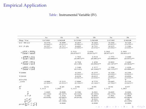
Empirical Application
Table : Instrumental Variable (IV).
1a 1b 2a 2b 3a 3b
Dep. Var. LCOH LMAR LCOH LMAR LCOH LMAR LU_M (𝛼) 0.574 0.599 0.267 0.164 0.556 0.728 (0.044)** (0.053)** (0.086)** (0.074)* (0.095)** (0.070)** LU_F (β) 0.527 0.717 0.682 0.731 0.915 1.186 (0.042)** (0.052)** (0.089)** (0.070)** (0.090)** (0.058)**
𝐿𝐻𝐻 ∗𝑀𝑀𝐻𝑀 ∗𝑀𝐻 2.315
(0.079)** 2.436 (0.073)**
2.282 (0.071)**
2.393 (0.051)**
𝐿𝑀𝑀 ∗ 𝐿𝐿𝐿𝑀 ∗𝑀𝐿 1.783
(0.087)** 2.514
(0.081)** 1.773
(0.080)** 2.440
(0.051)**
𝐿𝐻𝑀 ∗𝑀𝐿𝑀𝑀 ∗ 𝐻𝐿 0.784
(0.149) 1.430
(0.092)** 0.802
(0.147)** 2.440
(0.064)**
𝐿𝑀𝐻 ∗ 𝐿𝑀𝑀𝑀 ∗ 𝐿𝐻 1.340
(0.141) 1.377
(0.104)** 1.350
(0.135)** 1.428
(0.086)** Y2000 0.293 -0.277 0.320 -0.258 (0.042)** (0.035)** (0.038)** (0.025)** Y2010 0.624 -0.612 0.607 -0.694 (0.041)** (0.038)** (0.039)** (0.030)** STATE Y Y _cons -4.806 -5.215 -2.806 0.775 -8.045 -8.216 (0.384)** (0.452)** (0.196)** (0.180)** (0.798)** (0.663)** R2 0.51 0.45 0.90 0.95 0.92 0.97 N 1,113 1,283 1,113 1,283 1,113 1,283
𝛼𝛽 1.045
(0.132) 0.808
(0.107) 0.346
(0.165) 0.201
(0.103) 0.605
(0.135) 0.606
(0.065) 𝛼 + 𝛽 1.102 1.316 0.950 0.892 1.501 1.908
(0.038) (0.045) (0.018) (0.016) (0.082) (0.064) 𝛼ℳ
𝛽ℳ𝛽𝒞
𝛼𝒞
0.771 (0.140)
0.521 (0.347)
1.00 (0.249)
𝑝𝑟𝑜𝑏 𝛼ℳ = 𝛼𝒞
𝛽ℳ = 𝛽𝒞
0.000 0.090 0.000
* p<0.05; ** p<0.01
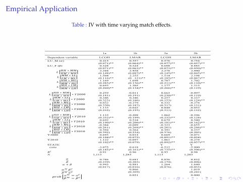
Empirical Application
Table : IV with time varying match effects.
1a 1b 2a 2b
Dependent variable LCOH LMAR LCOH LMAR LU_M (𝛼) 0.415 0.357 0.576 0.754 (0.071)** (0.064)** (0.077)** (0.057)** LU_F (β) 0.528 0.524 0.688 0.885 (0.071)** (0.063)** (0.073)** (0.050)**
𝐿𝐻𝐻 ∗𝑀𝑀𝐻𝑀 ∗𝑀𝐻
2.288
(0.148)** 2.458
(0.087)** 2.278
(0.145)** 2.440
(0.045)**
𝐿𝑀𝑀 ∗ 𝐿𝐿𝐿𝑀 ∗𝑀𝐿
1.504
(0.116)** 2.255
(0. .121)** 1.514
(0.103)** 2.198
(0.067)**
𝐿𝐻𝑀 ∗𝑀𝐿𝑀𝑀 ∗ 𝐻𝐿
1.169
(0.283)** 1.698
(0.136)** 0.787
(0.211)** 1.702
(0.110)**
𝐿𝑀𝐻 ∗ 𝐿𝑀𝑀𝑀 ∗ 𝐿𝐻
0.693
(0.260)** 1.305
(0.134)** 1.177
(0.266)** 1.313
(0.119)
𝐿𝐻𝐻 ∗𝑀𝑀𝐻𝑀 ∗𝑀𝐻
∗ 𝑌2000 0.259
(0.181) -0.011 (0.191)
0.663 (0.230)**
-0.097 (0.119)
𝐿𝑀𝑀 ∗ 𝐿𝐿𝐿𝑀 ∗𝑀𝐿
∗ 𝑌2000 0.346
(0.323) 0.346
(0.186) 0.257
(0.153) 0.337
(0.124)**
𝐿𝐻𝑀 ∗𝑀𝐿𝑀𝑀 ∗ 𝐻𝐿
∗ 𝑌2000 0.032
(0.330) -0.279 (0.187)
0.332 (0.317)
-0.274 (0.151)
𝐿𝑀𝐻 ∗ 𝐿𝑀𝑀𝑀 ∗ 𝐿𝐻
∗ 𝑌2000 1.133
(0.252) -0.042 (0.193)
0.040 (0.311)
-0.052 (0.152)
𝐿𝐻𝐻 ∗𝑀𝑀𝐻𝑀 ∗𝑀𝐻
∗ 𝑌2010 1.133
(0.252)** -0.208 (0.199)
1.062 (0.232)**
-0.396 (0.128)
𝐿𝑀𝑀 ∗ 𝐿𝐿𝐿𝑀 ∗𝑀𝐿
∗ 𝑌2010 0.692
(0.190)** 0.534
(0.200)** 0.679
(0.181)** 0.540
(0.162)**
𝐿𝐻𝑀 ∗𝑀𝐿𝑀𝑀 ∗ 𝐻𝐿
∗ 𝑌2010 -0.384 (0.261)
-0.609 (0.268)**
-0.323 (0.261)
-0.655 (0.246)**
𝐿𝑀𝐻 ∗ 𝐿𝑀𝑀𝑀 ∗ 𝐿𝐻
∗ 𝑌2010 0.394
(0.392) 0.264
(0.234) 0.391
(0.376) 0.237
(0.203) Y2000 0.693 0.014 0.669 -0.071 (0.104)** (0.075) (0.091)** (0.054) Y2010 1.122 -0.097 1.061 -0.274 (0.102)** (0.079) (0.092)** (0.057)** STATE Y Y _cons -3.075 0.618 -6.512 -5.900 (0.185)** (0.161)** (0.735)** (0.506)** R2 0.91 0.96 0.93 0.98 N 1,113 1,283 1,113 1,283
𝛼𝛽
0.786 (0.239)
0.681 (0.203)
0.836 (0.174)
0.852 (0.096)
𝛼 + 𝛽 0.943 0.881 1.264 1.640 (0.017) (0.016) (0.076) (0.055)
𝛼ℳ
𝛽ℳ𝛽𝒞
𝛼𝒞
0.866 (0.369)
1.019 (0.241)
𝑝𝑟𝑜𝑏 𝛼ℳ = 𝛼𝒞
𝛽ℳ = 𝛽𝒞
0.051 0.000

Conclusion
We propose a new static empirical marriage matching function (MMF):the Cobb Douglas MMF
The Cobb Douglas MMF encompasses CS, CSW, CSFT, CSPE, DM MMF
Properties of this Cobb Douglas MMF are presented.
Existence and uniqueness proof of the marriage distribution areprovided.
Comparative statistics are derived.

Conclusion
The CD MMF is estimated on US marriage and cohabitation data bystates from 1990 to 2010.
CS with peer effects is not rejected.
There are peer and scale effects in the US marriage markets.
We find evidence against all existing MMFs present so far in theliterature.
Positive assortative matching in marriage and cohabitation byeducational attainment are relatively stable from 1990 to 2010.