Cognitive Robotics SLAM with Lasers - Politecnico di Milanohome.deib.polimi.it/gini/robot/docs/Cognitive... · Cognitive Robotics –SLAM with Lasers Matteo Matteucci –[email protected]

Cognitive Robotics – SLAM with LasersMatteo Matteucci – [email protected]

Matteo Matteucci – [email protected]

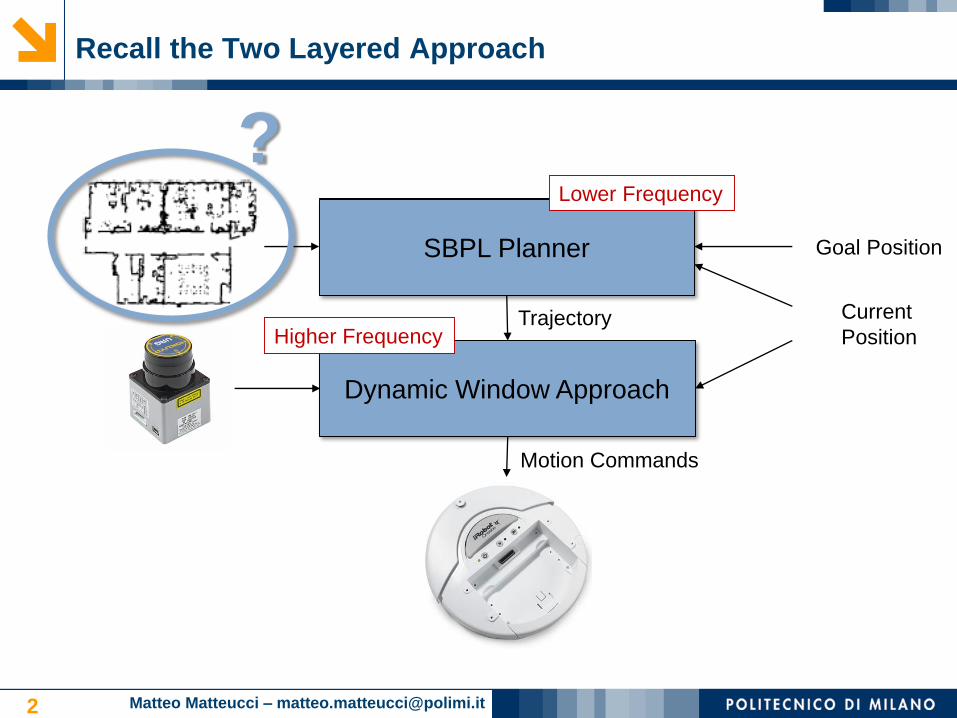
Recall the Two Layered Approach

2

Trajectory Planning

Trajectory Following

(and Obstacle Avoidance)

Goal Position

Current

PositionTrajectory

SBPL Planner

Lower Frequency

Motion Commands

Dynamic Window Approach

Higher Frequency

?


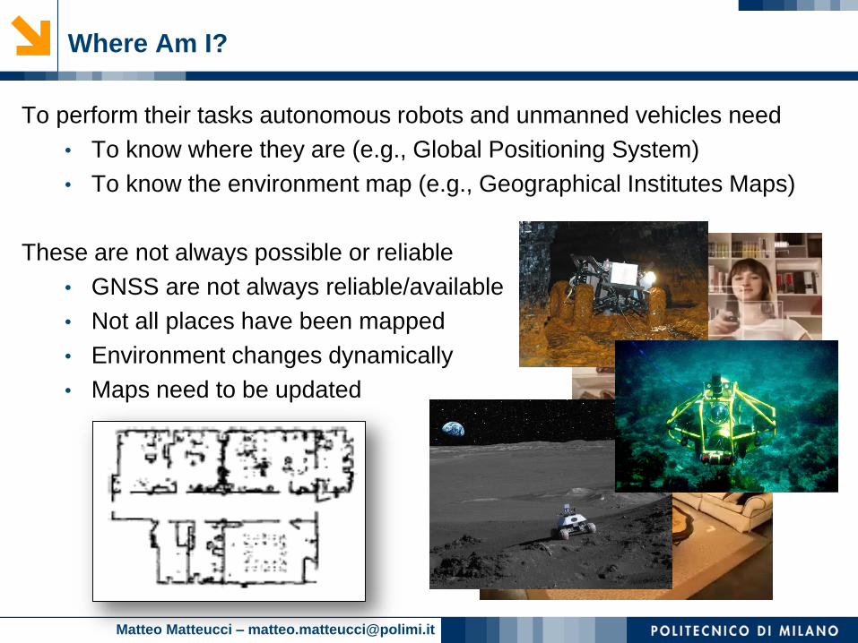
Where Am I?

To perform their tasks autonomous robots and unmanned vehicles need

• To know where they are (e.g., Global Positioning System)

• To know the environment map (e.g., Geographical Institutes Maps)

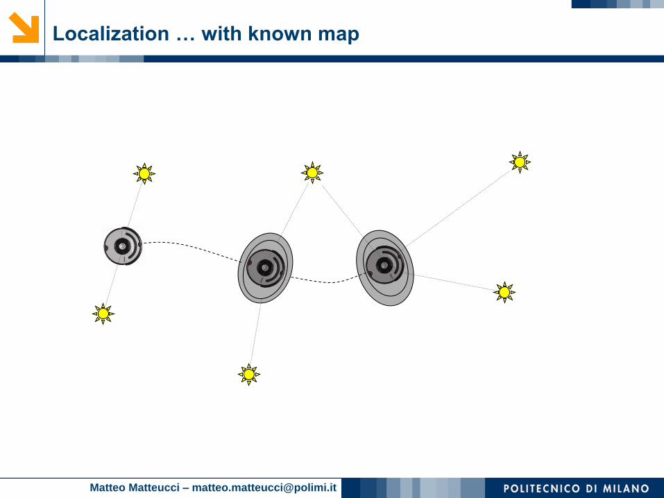
These are not always possible or reliable

• GNSS are not always reliable/available

• Not all places have been mapped

• Environment changes dynamically

• Maps need to be updated


Localization … with known map


Mapping … with known poses


Simultaneous Localization and Mapping


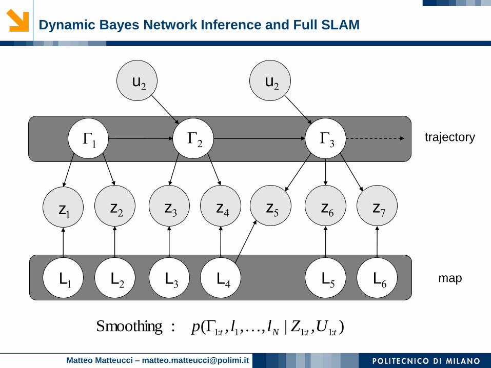
Dynamic Bayes Network Inference and Full SLAM

L1

G1

z1

G2

u2

),|,,,(:Smoothing :1:11:1 ttNt UZllp G

map

z2

L2 L3

z3 z4

L4

G3

u2

L5

z6 z7

L6

z5

trajectory


GG1:1

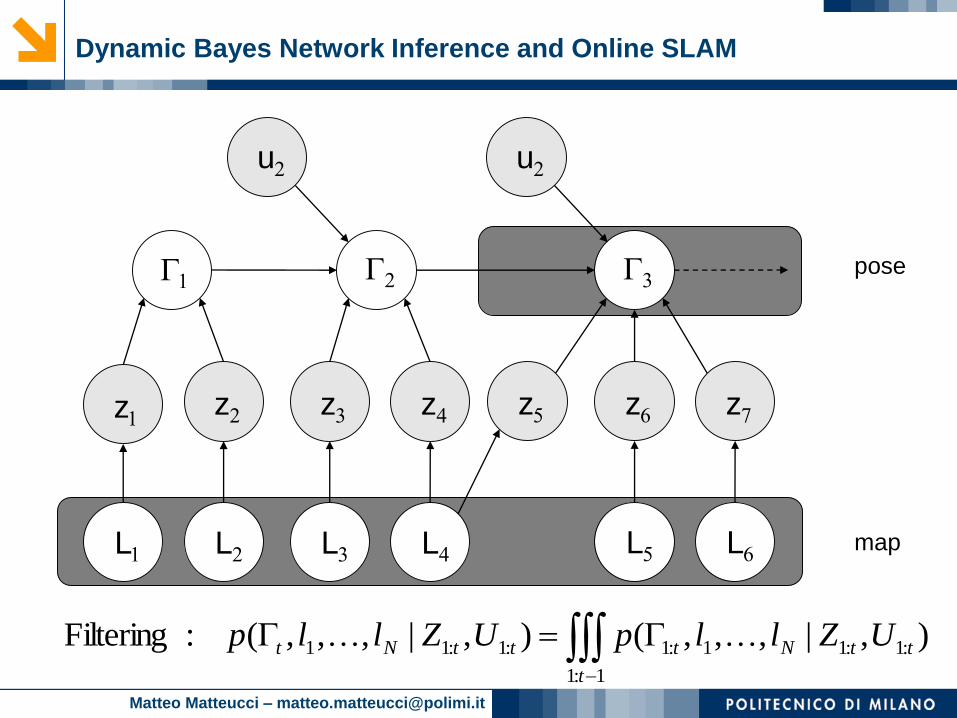
:1:11:1:1:11 ),|,,,(),|,,,(:Filteringt

ttNtttNt UZllpUZllp

Dynamic Bayes Network Inference and Online SLAM

L1

G1

z1

G2

u2

map

z2

L2 L3

z3 z4

L4

G3

u2

L5

z6 z7

L6

z5

pose


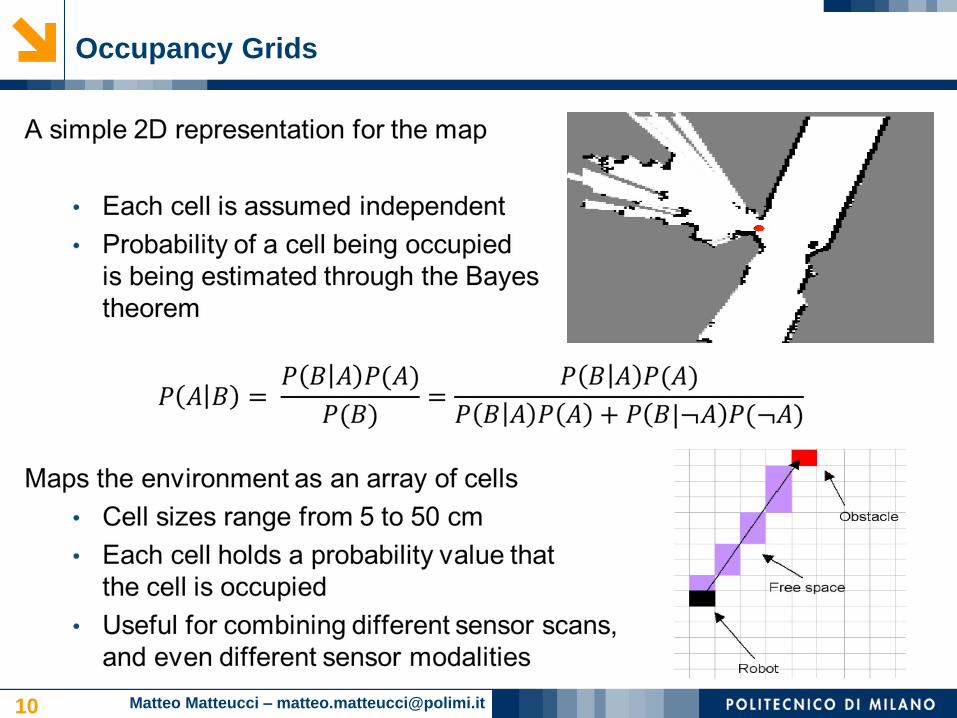
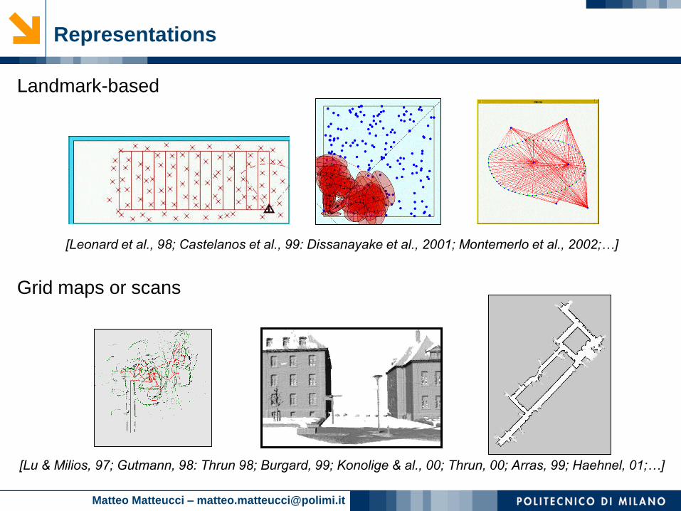
Representations

Landmark-based

[Leonard et al., 98; Castelanos et al., 99: Dissanayake et al., 2001; Montemerlo et al., 2002;…]

Grid maps or scans

[Lu & Milios, 97; Gutmann, 98: Thrun 98; Burgard, 99; Konolige & al., 00; Thrun, 00; Arras, 99; Haehnel, 01;…]


Occupancy Grids

10


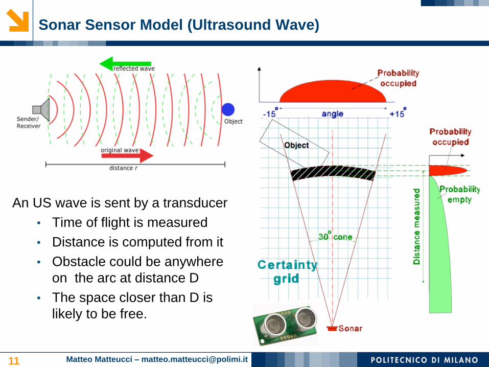
Sonar Sensor Model (Ultrasound Wave)

An US wave is sent by a transducer

• Time of flight is measured

• Distance is computed from it

• Obstacle could be anywhere

on the arc at distance D

• The space closer than D is

likely to be free.

11


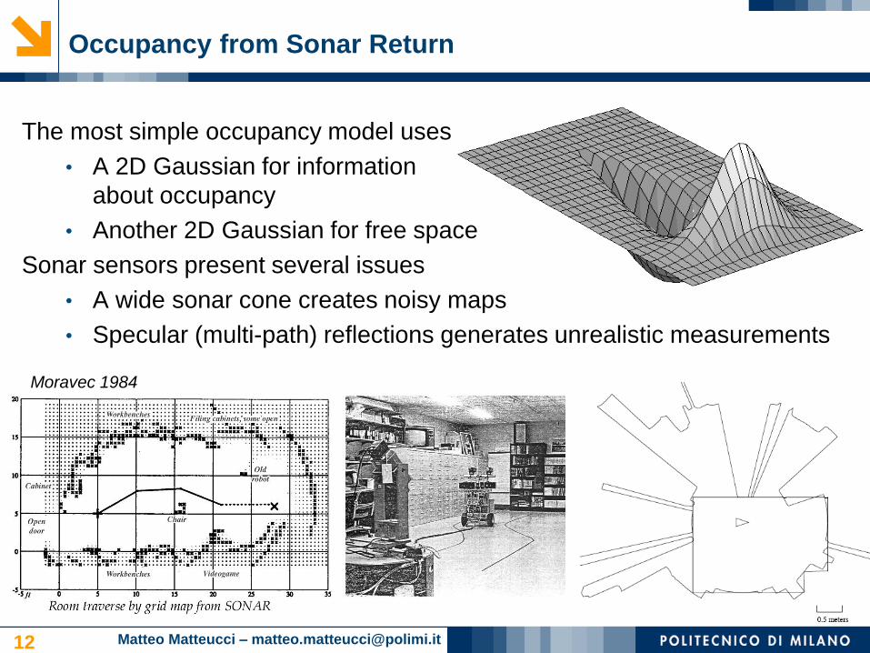
Occupancy from Sonar Return

The most simple occupancy model uses

• A 2D Gaussian for information

about occupancy

• Another 2D Gaussian for free space

Sonar sensors present several issues

• A wide sonar cone creates noisy maps

• Specular (multi-path) reflections generates unrealistic measurements

12

Moravec 1984


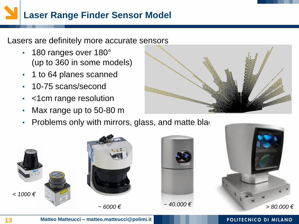
Laser Range Finder Sensor Model

Lasers are definitely more accurate sensors

• 180 ranges over 180°

(up to 360 in some models)

• 1 to 64 planes scanned

• 10-75 scans/second

• <1cm range resolution

• Max range up to 50-80 m

• Problems only with mirrors, glass, and matte black.

13

< 1000 €

> 80.000 €~ 40.000 €~ 6000 €


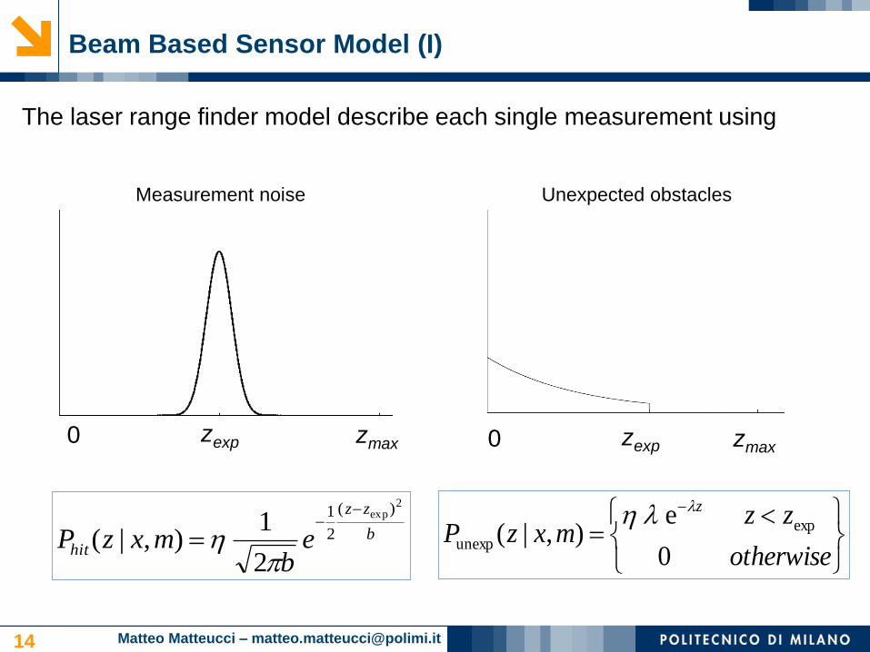
Beam Based Sensor Model (I)

The laser range finder model describe each single measurement using

14

Measurement noise

zexp zmax0

b

zz

hit eb

mxzP

2exp)(

2

1

2

1),|(

otherwise

zzmxzP

z

0

e),|( exp

unexp

Unexpected obstacles

zexp zmax0


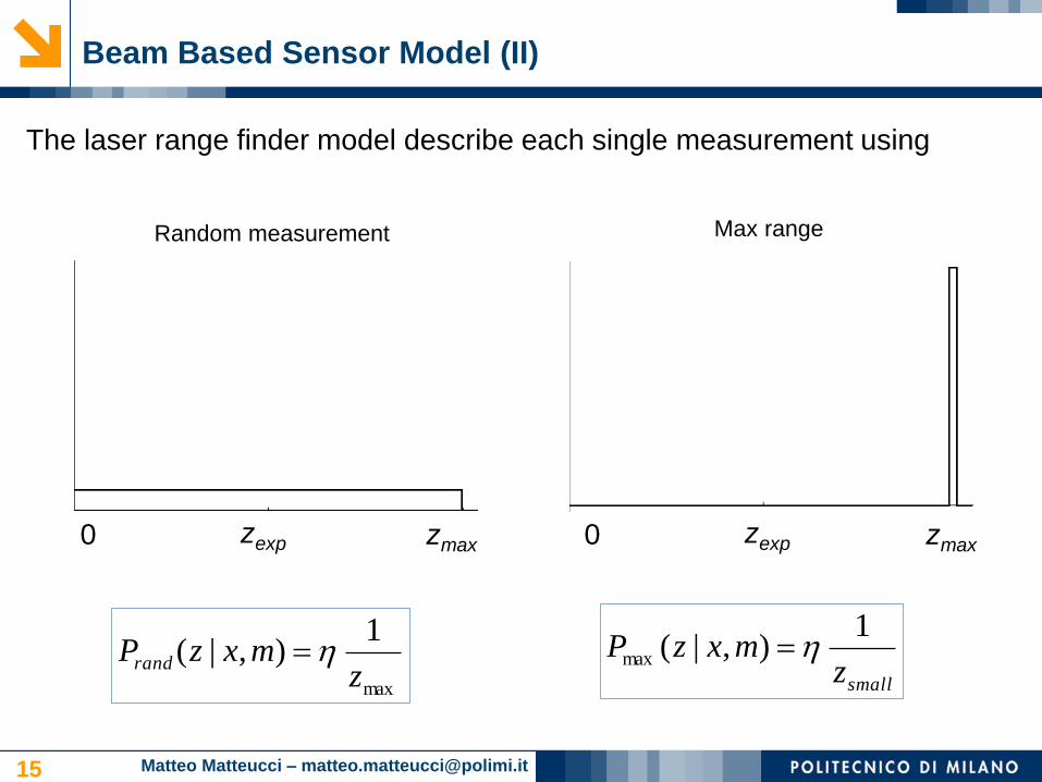
Beam Based Sensor Model (II)


15

Random measurement Max range

max

1),|(

zmxzPrand

smallzmxzP

1),|(max

zexp zmax0zexp zmax0


Beam Based Sensor Model (III)


Which, is practice, turns out to be

quite accurate!

16

),|(

),|(

),|(

),|(

),|(

rand

max

unexp

hit

rand

max

unexp

hit

mxzP

mxzP

mxzP

mxzP

mxzP

T


Occupancy Grid Cell Update

17


Occupancy by Log Odds

18


Mapping with Raw Odometry (with known poses)


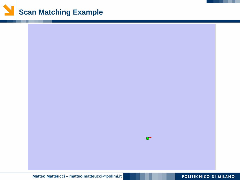
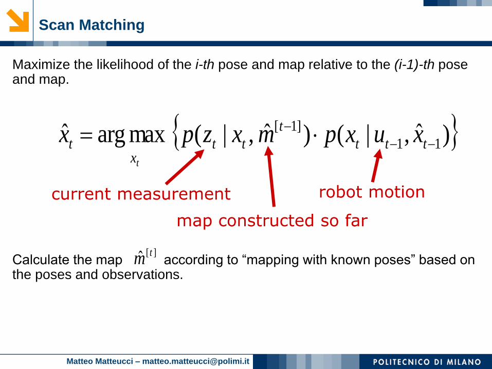
Scan Matching

Maximize the likelihood of the i-th pose and map relative to the (i-1)-th pose and map.

Calculate the map according to “mapping with known poses” based on the poses and observations.

)ˆ,|( )ˆ ,|( maxargˆ11

]1[

ttt

t

ttx

t xuxpmxzpxt

robot motioncurrent measurement

map constructed so far

][ˆ tm


Scan Matching Example


Techniques for Generating Consistent Maps

Several techniques have been studied to obtain a consistent estimate of the

joint probability of pose and map

Scan matching

EKF SLAM / UKF SLAM

Fast-SLAM (Particle filter based)

Probabilistic mapping with a single map and a posterior about poses

(Mapping + Localization)

Graph-SLAM, SEIFs

...

We won’t see the all of them!


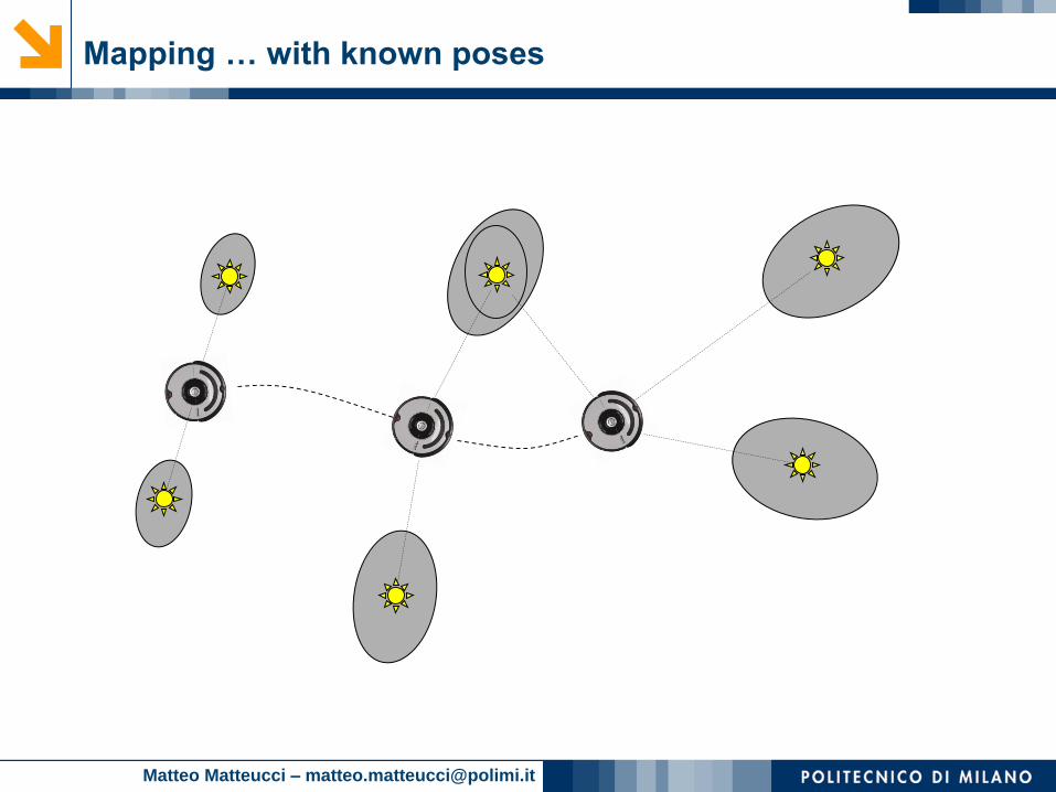
SLAM: Simultaneous Localization and Mapping

Full SLAM:

Online SLAM:

Integrations typically done one at a time

),|,( :1:1:1 ttt uzmxp

121:1:1:1:1:1 ...),|,(),|,( ttttttt dxdxdxuzmxpuzmxp

Estimates most recent pose and map!

Estimates entire path and map!

Two famous example of this!

Extended Kalman Filter (EKF) SLAM

• Solves online SLAM problem

• Uses a linearized Gaussian probability distribution model

FastSLAM

• Solves full SLAM problem

• Uses a sampled particle filter distribution model


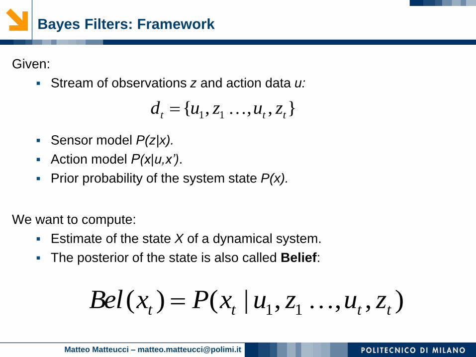
Bayes Filters: Framework

Given:

Stream of observations z and action data u:

Sensor model P(z|x).

Action model P(x|u,x’).

Prior probability of the system state P(x).

We want to compute:

Estimate of the state X of a dynamical system.

The posterior of the state is also called Belief:

),,,|()( 11 tttt zuzuxPxBel

},,,{ 11 ttt zuzud


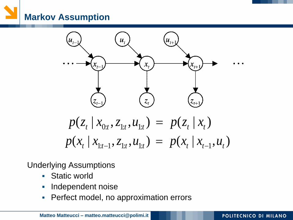
Markov Assumption

Underlying Assumptions

Static world

Independent noise

Perfect model, no approximation errors

),|(),,|( 1:1:11:1 ttttttt uxxpuzxxp

)|(),,|( :1:1:0 tttttt xzpuzxzp


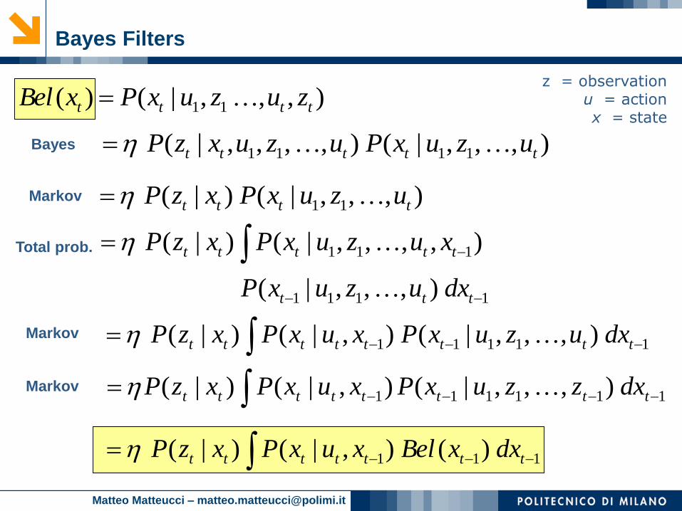
111 )(),|()|( ttttttt dxxBelxuxPxzP

Bayes Filters

),,,|(),,,,|( 1111 ttttt uzuxPuzuxzP Bayes

z = observationu = actionx = state

),,,|()( 11 tttt zuzuxPxBel

Markov ),,,|()|( 11 tttt uzuxPxzP

Markov11111 ),,,|(),|()|( tttttttt dxuzuxPxuxPxzP

1111

111

),,,|(

),,,,|()|(

ttt

ttttt

dxuzuxP

xuzuxPxzP

Total prob.

Markov111111 ),,,|(),|()|( tttttttt dxzzuxPxuxPxzP


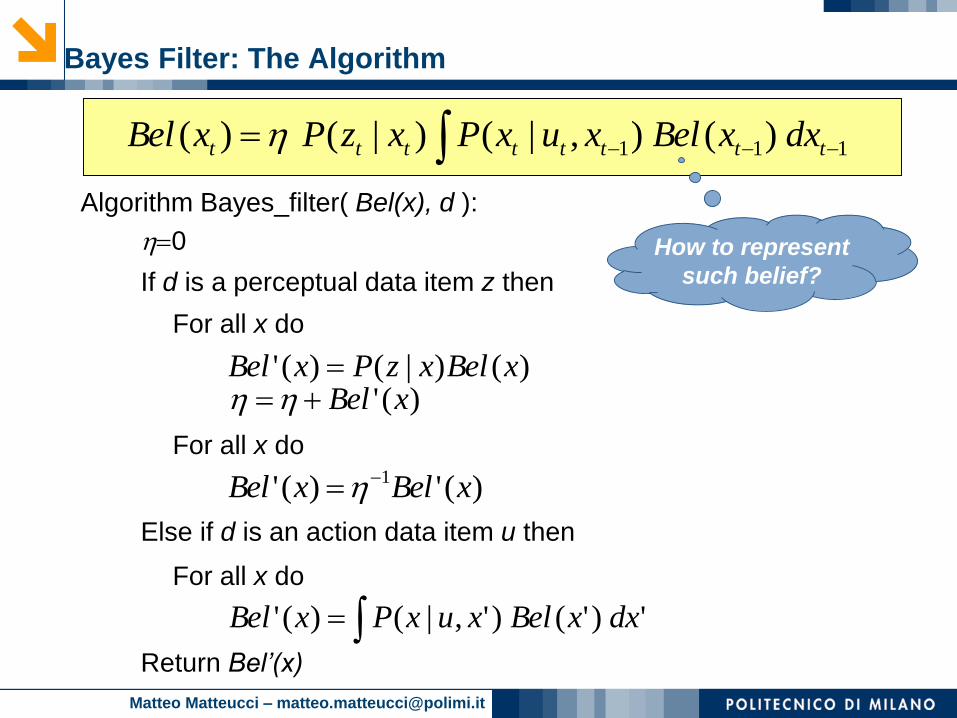
Bayes Filter: The Algorithm

Algorithm Bayes_filter( Bel(x), d ):

0

If d is a perceptual data item z then

For all x do

For all x do

Else if d is an action data item u then

For all x do

Return Bel’(x)

)()|()(' xBelxzPxBel )(' xBel

)(')(' 1 xBelxBel

')'()',|()(' dxxBelxuxPxBel

111 )(),|()|()( tttttttt dxxBelxuxPxzPxBel

How to represent

such belief?


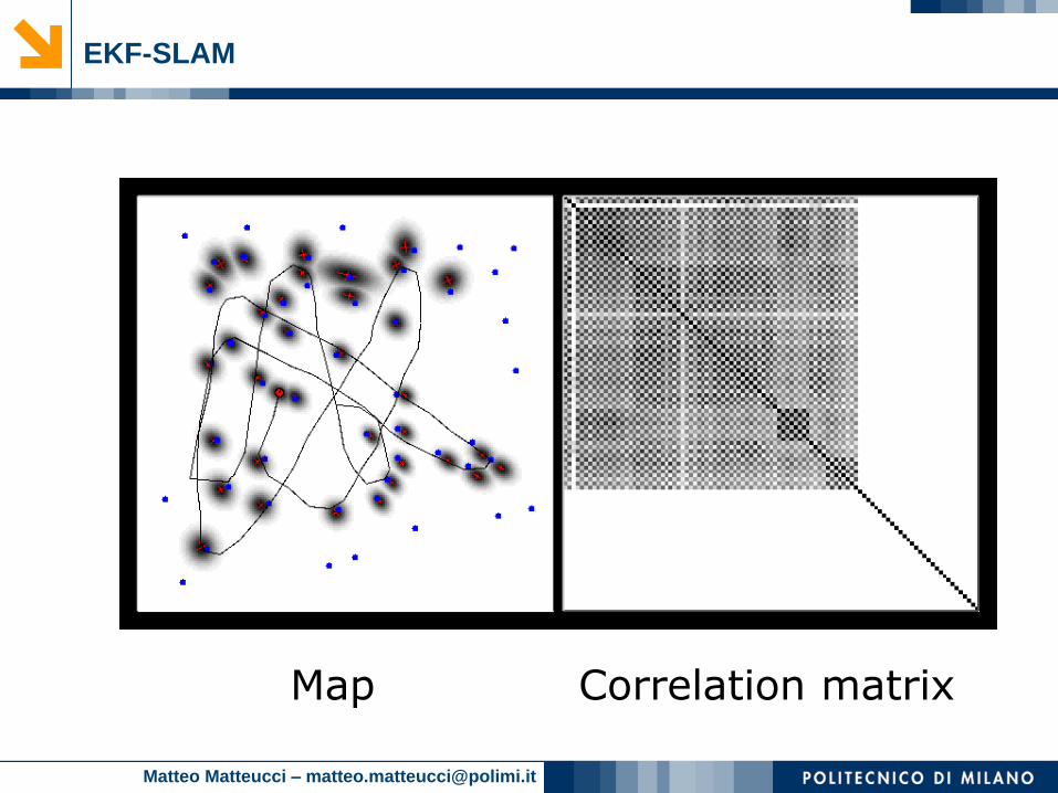
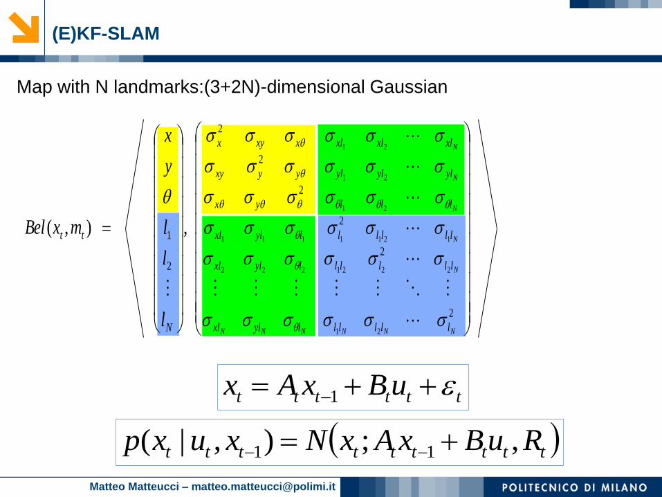
(E)KF-SLAM

Map with N landmarks:(3+2N)-dimensional Gaussian

2

2

2

2

2

2

2

1

21

2221222

1211111

21

21

21

,),(

NNNNNN

N

N

N

N

N

llllllylxl

llllllylxl

llllllylxl

lllyx

ylylylyyxy

xlxlxlxxyx

N

tt

l

l

l

y

x

mxBel

tttttt uBxAx 1

ttttttttt RuBxAxNxuxp ,;),|( 11


(E)KF-SLAM

Map with N landmarks:(3+2N)-dimensional Gaussian

2

2

2

2

2

2

2

1

21

2221222

1211111

21

21

21

,),(

NNNNNN

N

N

N

N

N

llllllylxl

llllllylxl

llllllylxl

lllyx

ylylylyyxy

xlxlxlxxyx

N

tt

l

l

l

y

x

mxBel

tttt xCz

tttttt QxCzNxzp ,;)|(


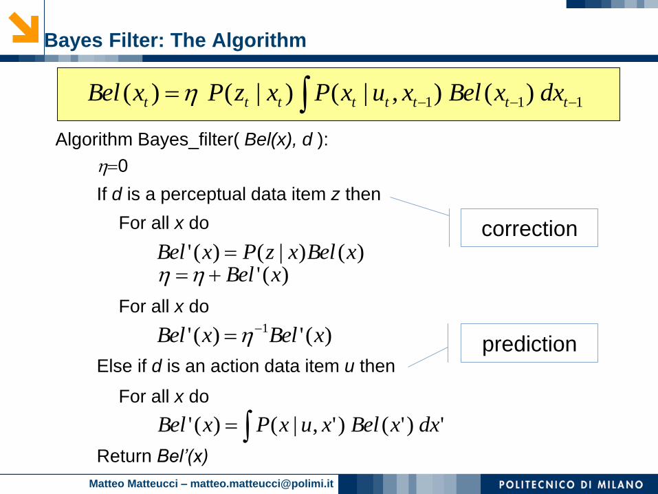
Bayes Filter: The Algorithm

Algorithm Bayes_filter( Bel(x), d ):

0

If d is a perceptual data item z then

For all x do

For all x do

Else if d is an action data item u then

For all x do

Return Bel’(x)

)()|()(' xBelxzPxBel )(' xBel

)(')(' 1 xBelxBel

')'()',|()(' dxxBelxuxPxBel

111 )(),|()|()( tttttttt dxxBelxuxPxzPxBel

prediction

correction


2

2

2

2

2

2

2

1

21

2221222

1211111

21

21

21

,),(

NNNNNN

N

N

N

N

N

llllllylxl

llllllylxl

llllllylxl

lllyx

ylylylyyxy

xlxlxlxxyx

N

tt

l

l

l

y

x

mxBel

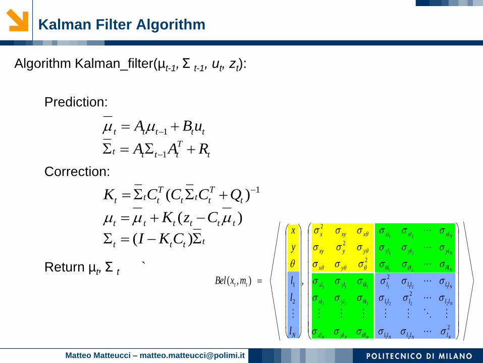
Kalman Filter Algorithm

Algorithm Kalman_filter(µt-1, Σ t-1, ut, zt):

Prediction:

Correction:

Return µt, Σ t `

ttttt uBA 1

t

T

tttt RAA 1

1)( t

T

ttt

T

ttt QCCCK

)( tttttt CzK

tttt CKI )(


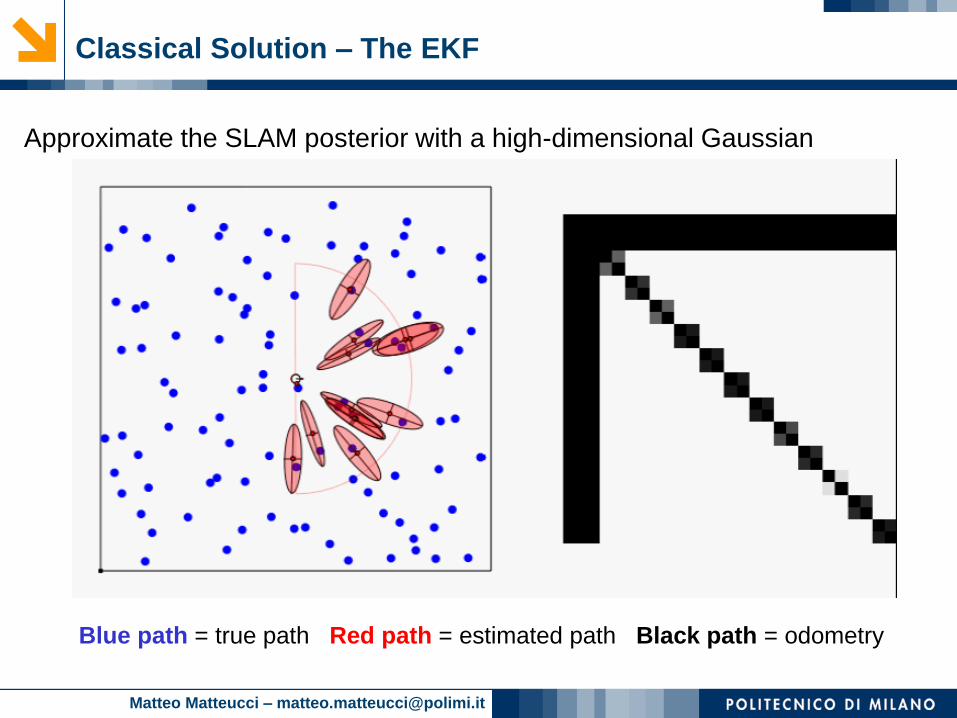
Classical Solution – The EKF

Approximate the SLAM posterior with a high-dimensional Gaussian

Blue path = true path Red path = estimated path Black path = odometry


EKF-SLAM

Map Correlation matrix


EKF-SLAM



EKF-SLAM



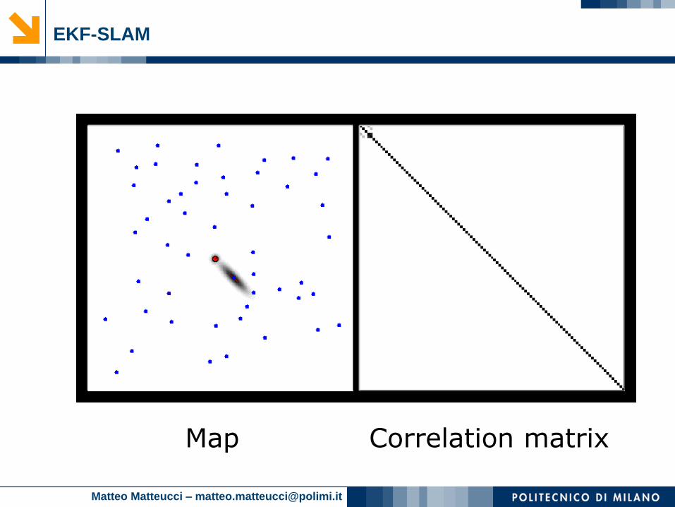
Properties of KF-SLAM (Linear Case)

Theorem:

The determinant of any sub-matrix of the map covariance matrix decreases

monotonically as successive observations are made.

Theorem:

In the limit the landmark estimates become fully correlated

[Dissanayake et al., 2001]

Are we happy about this?

• Quadratic in the number of landmarks: O(n2)

• Convergence results for the linear case.

• Can diverge if nonlinearities are large!

• Have been applied successfully in large-scale environments.

• Approximations reduce the computational complexity.


EKF Drawbacks

EKF-SLAM works pretty well but ...

• EKF-SLAM employs linearized models of nonlinear motion and

observation models and so inherits many caveats.

• Computational effort is demand because computation grows

quadratically with the number of landmarks.

Possible solutions

• Local submaps [Leonard & al 99, Bosse & al 02, Newman & al 03]

• Sparse links (correlations) [Lu & Milios 97, Guivant & Nebot 01]

• Sparse extended information filters [Frese et al. 01, Thrun et al. 02]

• Thin junction tree filters [Paskin 03]

• Rao-Blackwellisation (FastSLAM) [Murphy 99, Montemerlo et al. 02,

Eliazar et al. 03, Haehnel et al. 03]

• Represents nonlinear process and non-Gaussian uncertainty

• Rao-Blackwellized method reduces computation


Particle Filters

Represent belief by random samples

Estimation of non-Gaussian, nonlinear processes

• Monte Carlo filter

• Survival of the fittest

• Condensation

• Bootstrap filter

• Particle filter

• …

Filtering: [Rubin, 88], [Gordon et al., 93], [Kitagawa 96]

Computer vision: [Isard and Blake 96, 98]

Dynamic Bayesian Networks: [Kanazawa et al., 95]


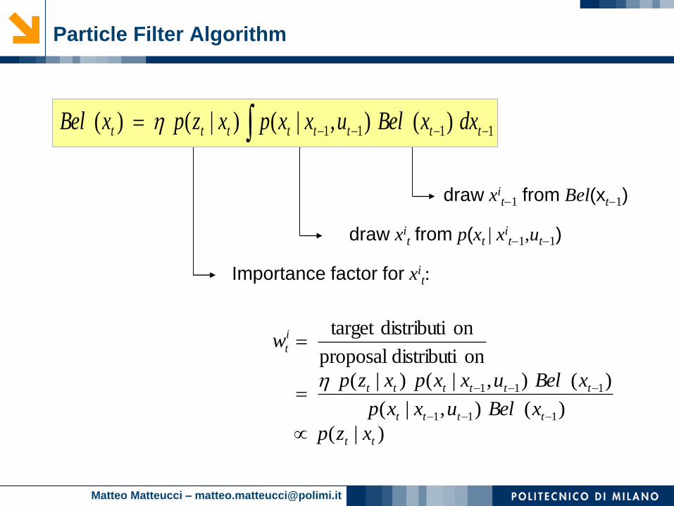
draw xit1 from Bel(xt1)

draw xit from p(xt | x

it1,ut1)

Importance factor for xit:

)|(

)(),|(

)(),|()|(

ondistributi proposal

ondistributitarget

111

111

tt

tttt

tttttt

i

t

xzp

xBeluxxp

xBeluxxpxzp

w

1111 )(),|()|()( tttttttt dxxBeluxxpxzpxBel

Particle Filter Algorithm


A Four Legged Example …

40


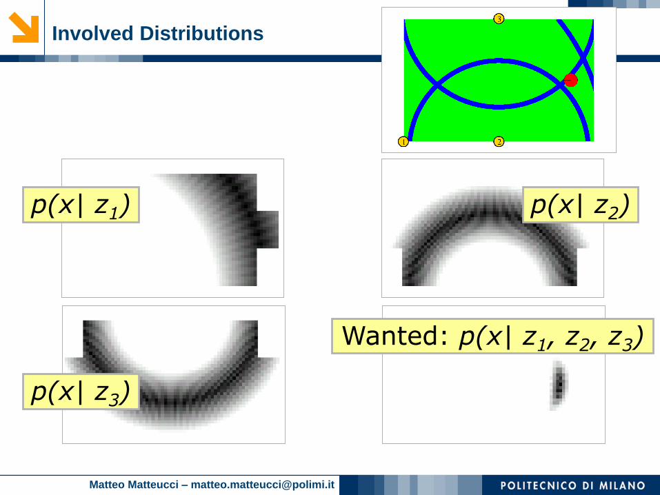
Involved Distributions

Wanted: p(x| z1, z2, z3)

p(x| z1) p(x| z2)

p(x| z3)


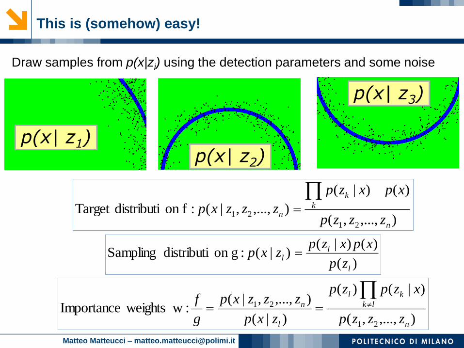
This is (somehow) easy!

Draw samples from p(x|zi) using the detection parameters and some noise

),...,,(

)()|(

),...,,|( :fon distributiTarget 21

21

n

k

k

nzzzp

xpxzp

zzzxp

)(

)()|()|( :gon distributi Sampling

l

ll

zp

xpxzpzxp

),...,,(

)|()(

)|(

),...,,|( : w weightsImportance

21

21

n

lk

kl

l

n

zzzp

xzpzp

zxp

zzzxp

g

f

p(x| z1)p(x| z2)

p(x| z3)


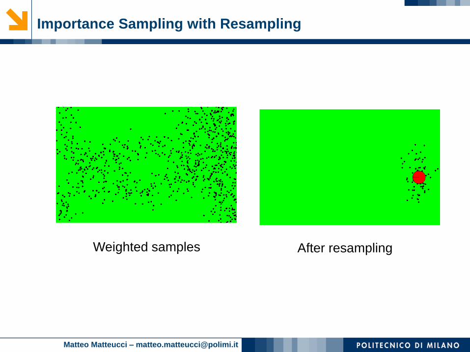
Weighted samples After resampling

Importance Sampling with Resampling


Localization for AIBO robots


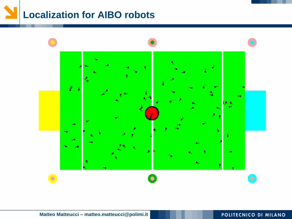
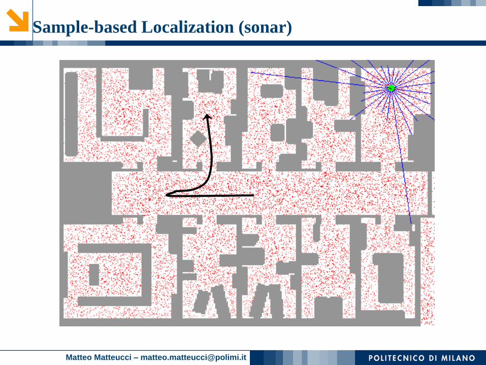
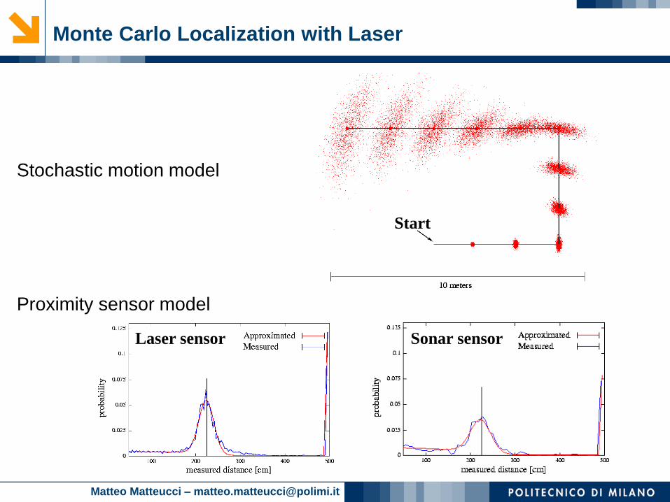
Start

Monte Carlo Localization with Laser

Stochastic motion model

Proximity sensor model

Laser sensor Sonar sensor


Sample-based Localization (sonar)


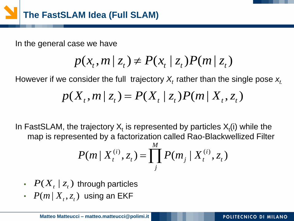
In the general case we have

However if we consider the full trajectory Xt rather than the single pose xt.

In FastSLAM, the trajectory Xt is represented by particles Xt(i) while the

map is represented by a factorization called Rao-Blackwellized Filter

• through particles

• using an EKF

The FastSLAM Idea (Full SLAM)

( , | ) ( | ) ( | , )t t t t t tp X m z P X z P m X z

( , | ) ( | ) ( | )t t t t tp x m z P x z P m z

( | , )t tP m X z

( | )t tP X z

( ) ( )( | , ) ( | , )M

i i

t t j t t

j

P m X z P m X z


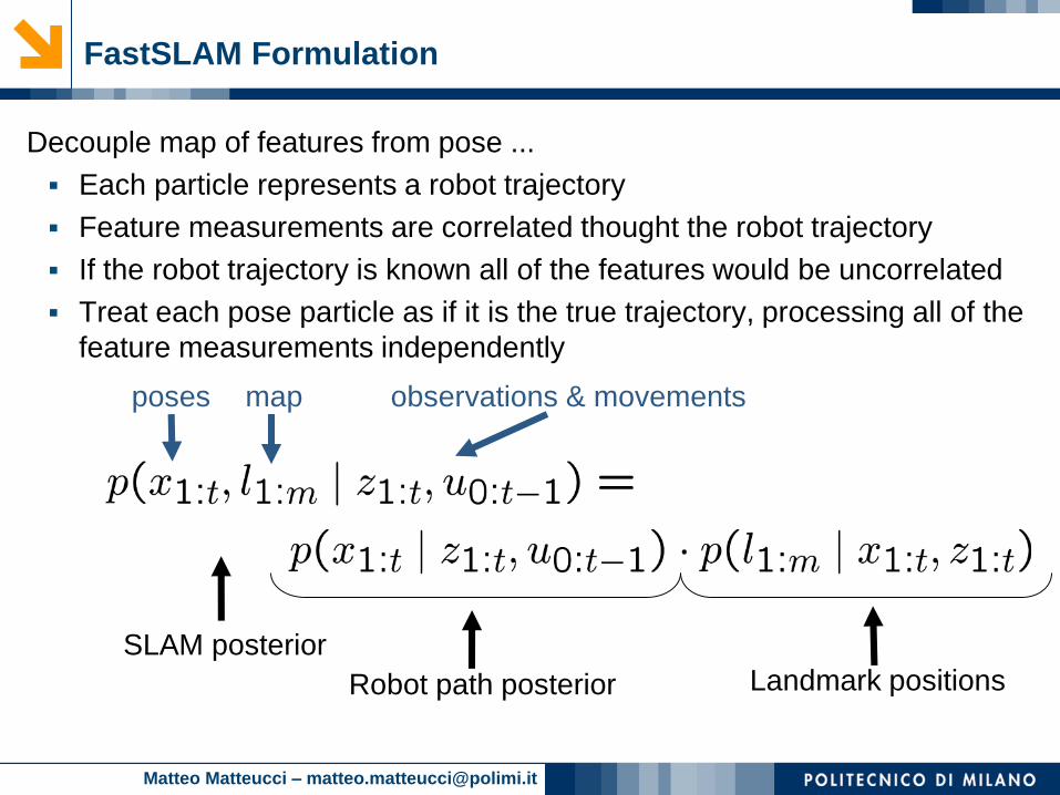
FastSLAM Formulation

Decouple map of features from pose ...

Each particle represents a robot trajectory

Feature measurements are correlated thought the robot trajectory

If the robot trajectory is known all of the features would be uncorrelated

Treat each pose particle as if it is the true trajectory, processing all of the

feature measurements independently

SLAM posterior

Robot path posterior Landmark positions

poses map observations & movements


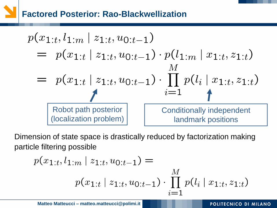
Factored Posterior: Rao-Blackwellization

Robot path posterior

(localization problem)Conditionally independent

landmark positions

Dimension of state space is drastically reduced by factorization making

particle filtering possible


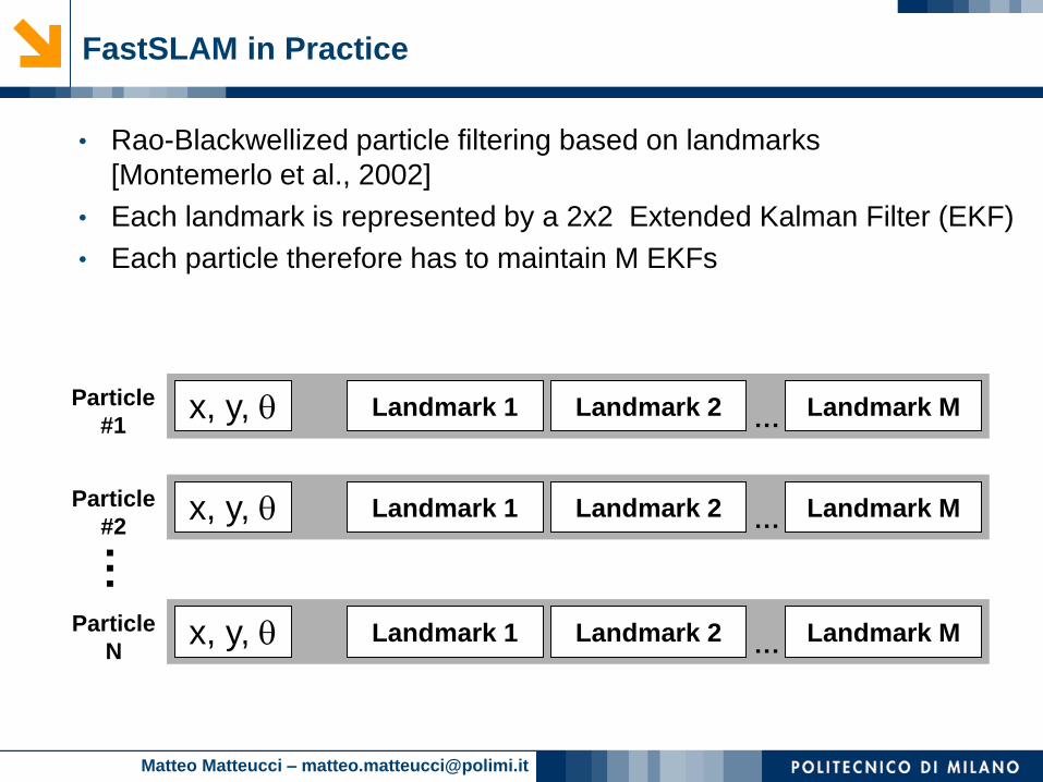
Landmark 1 Landmark 2 Landmark M…x, y,

Landmark 1 Landmark 2 Landmark M…x, y, Particle

#1

Landmark 1 Landmark 2 Landmark M…x, y, Particle

#2

Particle

N

…

FastSLAM in Practice

• Rao-Blackwellized particle filtering based on landmarks

[Montemerlo et al., 2002]

• Each landmark is represented by a 2x2 Extended Kalman Filter (EKF)

• Each particle therefore has to maintain M EKFs


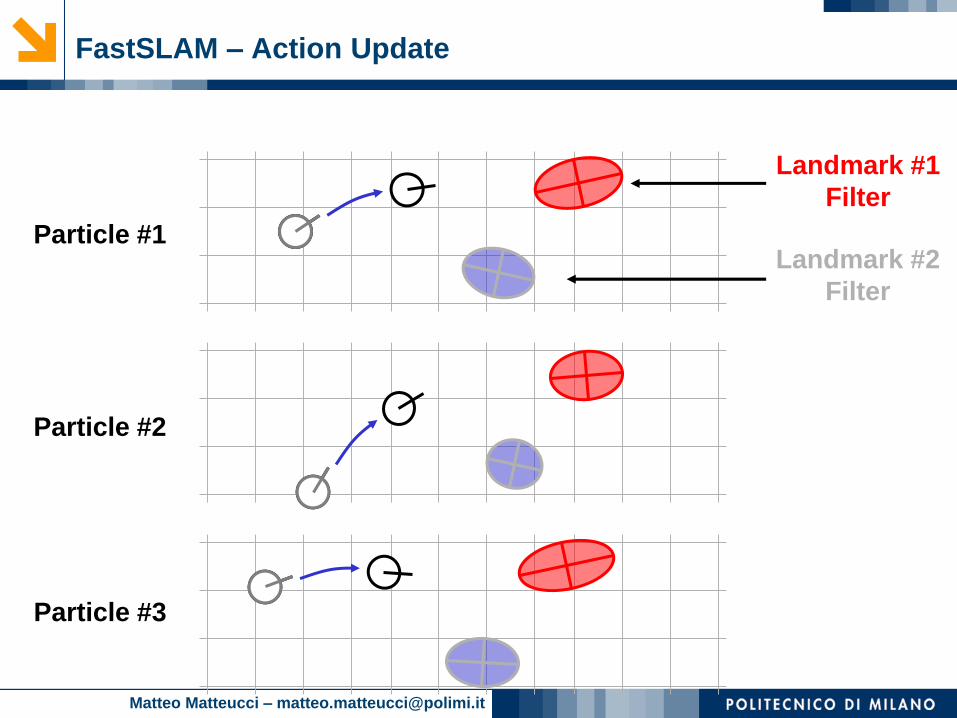
FastSLAM – Action Update

Particle #1

Particle #2

Particle #3

Landmark #1

Filter

Landmark #2

Filter


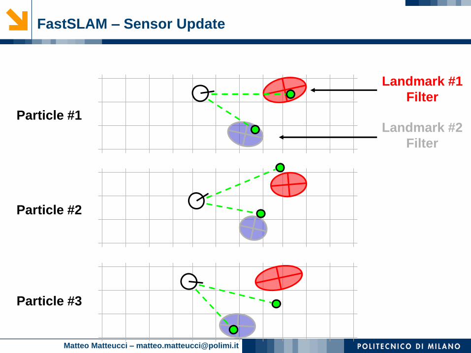
FastSLAM – Sensor Update

Particle #1

Particle #2

Particle #3

Landmark #1

Filter

Landmark #2

Filter


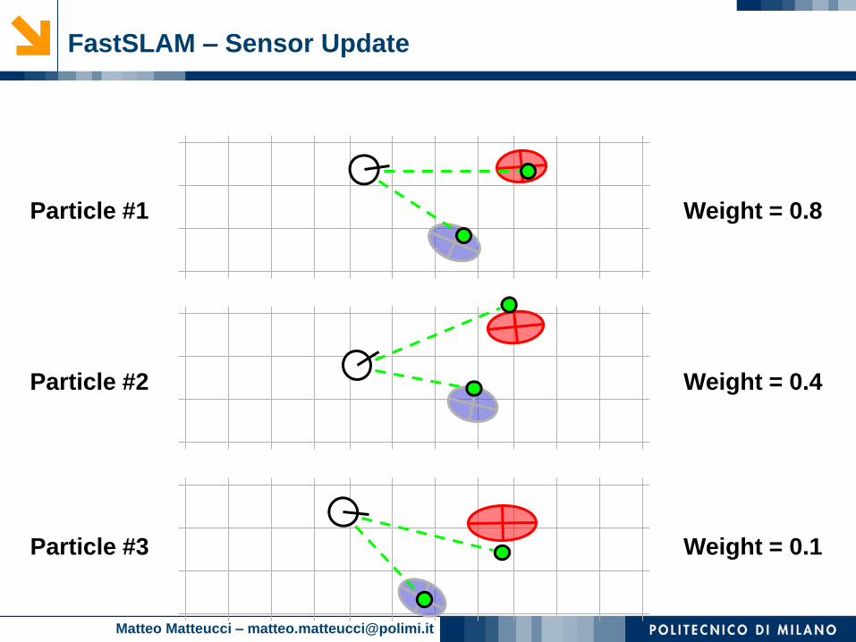
FastSLAM – Sensor Update

Particle #1

Particle #2

Particle #3

Weight = 0.8

Weight = 0.4

Weight = 0.1


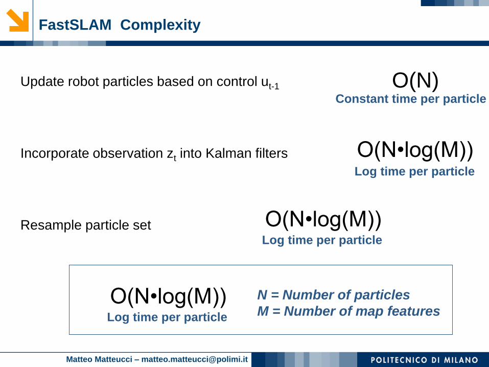
FastSLAM Complexity

Update robot particles based on control ut-1

Incorporate observation zt into Kalman filters

Resample particle set

N = Number of particles

M = Number of map features

O(N)Constant time per particle

O(N•log(M))Log time per particle




Fast-SLAM Example


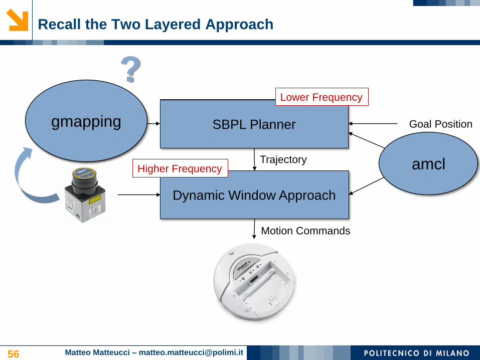
Recall the Two Layered Approach

56

Trajectory Planning

Trajectory Following

(and Obstacle Avoidance)

Goal Position

Current

PositionTrajectory

SBPL Planner

Lower Frequency

Motion Commands

Dynamic Window Approach

Higher Frequency

?

gmapping

amcl

Cognitive Robotics –SLAM with LasersMatteo Matteucci – [email protected]

Documents

Cognitive Robotics SLAM with Lasers - Politecnico di Milanohome.deib.polimi.it/gini/robot/docs/Cognitive... · Cognitive Robotics –SLAM with Lasers Matteo Matteucci –[email protected]