Embed Size (px)
Citation preview

Coffee Can Radar: Detection and Jamming
A Major Qualifying Project
Submitted to the faculty of
WORCESTER POLYTECHNIC INSTITUTE
In partial fulfillment of the requirements
for the Degree of Bachelor of Science
Gabriela de Peralta
Electrical and Computer Engineering 2017
Michael J. Inserra
Electrical and Computer Engineering 2017
Daniella Morico
Electrical and Computer Engineering 2017
Project Advisor:
Professor Alexander M. Wyglinski
Department of Electrical and Computer Engineering
This report represents work of WPI undergraduate students
submitted to the faculty as evidence of a degree requirement. WPI
routinely publishes these reports on its web site without editorial or
peer review. For more information about the projects program at
WPI, see http://www.wpi.edu/Academics/Projects.

1
Abstract
This project models the operation of an interception-resistant automotive radar and demonstrates
its susceptibility to jamming. The initial hardware design was based on open courseware from MIT
Lincoln Laboratory. Prior to the construction of the radar, expected results were recorded using
MATLAB and LTspice simulations. The interference signals were designed in MATLAB and
transmitted using a software-defined radio. Final testing was completed using a spectrum analyzer
and software designed to plot the time-lapsed location of a detected object.

2
Acknowledgements
The team would like to thank many people for their guidance and assistance throughout the
duration of this project, especially Professor Wyglinski for the project motivation, constant
positive support, and recommendations for system troubleshooting. The team would also like to
thank Professor John McNeill for the opportunity to conduct our research and design under his
laboratory, NECAMSID. Additionally, we would like to thank Denver Cohen and Calvin
Figuereo-Supraner for their troubleshooting skills, schematic designs, and programming assistance
in MATLAB. Lastly, we would like to thank Professor Makarov for his assistance in discussing
antenna design and using a spectrum analyzer during testing.

3
Table of Contents Abstract ........................................................................................................................................... 1
Acknowledgements ......................................................................................................................... 2
Table of Contents ............................................................................................................................ 3
List of Figures ................................................................................................................................. 4
List of Tables .................................................................................................................................. 5
1 Introduction .................................................................................................................................. 6
1.1 Current State of the Art ......................................................................................................... 7
1.2 Problem Statement ................................................................................................................ 9
1.3 Proposed Solution and Design Effort .................................................................................... 9
1.4 Report Organization ............................................................................................................ 10
2 Radar Fundamentals................................................................................................................... 11
2.1 Radar Jamming .................................................................................................................... 13
2.2 Signal Processing Techniques ............................................................................................. 15
2.3 Component Research........................................................................................................... 17
2.4 Automotive Radar ............................................................................................................... 22
2.5 Chapter Summary ................................................................................................................ 24
3 Proposed Approach .................................................................................................................... 25
3.1 Candidate Designs ............................................................................................................... 25
3.2 Gantt Chart Development.................................................................................................... 26
4.1 Build Procedure ................................................................................................................... 30
4.2 Simulations .......................................................................................................................... 38
4.3 Test Procedure ..................................................................................................................... 43
4.4 Chapter Summary ................................................................................................................ 48
5 Experimental Results ................................................................................................................. 49
5.1 Full System Operation ......................................................................................................... 49
5.2 Chapter Summary ................................................................................................................ 56
6 Conclusions ................................................................................................................................ 57
6.1 Future Work ........................................................................................................................ 58
Appendices .................................................................................................................................... 59
Appendix A: Cost of Materials ................................................................................................. 59
Appendix B: MATLAB Code ................................................................................................... 61
References ..................................................................................................................................... 68

4
List of Figures Figure 1. Radar Block Diagram ..................................................................................................... 8
Figure 2. Autonomous Vehicle Conceptual Diagram Component Explanations ........................... 9
Figure 3. Searching Radar Block Diagram ................................................................................... 18
Figure 4. Video Amplifier Analog Circuitry Schematic ............................................................... 21
Figure 5. Modulator Analog Circuitry Schematic ........................................................................ 22
Figure 6. Autonomous Vehicle Forward-Facing Radar Mounting System (Bumper-Integrated) 24
Figure 8. RF Chain Assembly ....................................................................................................... 30
Figure 9. Protoboard Mounting..................................................................................................... 31
Figure 10. Completed Searching Can Radar................................................................................. 32
Figure 11. Pluto SDR .................................................................................................................... 33
Figure 12. Relative Power Measurement of FMCW Radar Signal .............................................. 34
Figure 13. Frequency Bandwidth Measurement of FMCW Radar ............................................... 34
Figure 14. FMCW Radar Signal vs SDR-generated Noise Power ............................................... 35
Figure 15. Band-Limited Noise Signal Interference ..................................................................... 36
Figure 16. Magnitude Response of Bandpass Filter ..................................................................... 38
Figure 17. Modulator Circuit in LTspice ...................................................................................... 39
Figure 18. Modulator Waveforms................................................................................................. 39
Figure 19. 5-50 Hz FMCW Chirp with Mean Squared Error ....................................................... 40
Figure 20. 5-50 kHz FMCW Chirp with Mean Squared Error ..................................................... 41
Figure 21. 50-500 kHz FMCW Chirp with Mean Squared Error ................................................. 42
Figure 22. 50-500 MHz FMCW Chirp with Mean Squared Error ............................................... 43
Figure 23. Baseline Calibration Magnitude Response of Spectrum Analyzer with 50 Ω Input ... 45
Figure 24. Tuning of Transmit Antenna -12 dB Resonance ......................................................... 45
Figure 25. Tuning of Receive Antenna -20 dB Resonance .......................................................... 46
Figure 26. Initial Radar System Test ............................................................................................ 47
Figure 27. Radar System Test with Pluto SDRs ........................................................................... 48
Figure 28. Radar Reading of Person Walking in AK227 Test #1 ................................................ 50
Figure 29. Radar Reading of Person Walking in AK227 Test # 2 ............................................... 50
Figure 31. Test Between Salisbury Street and WPI Fountain ...................................................... 51
Figure 32. WPI Fountain and Walkway towards Salisbury Street ............................................... 52
Figure 33. Walking Test with Metal Sheet ................................................................................... 52
Figure 34. Walkway In Front of Atwater Kent Laboratories ........................................................ 53
Figure 35. Radar Jammed Using Metal Tin .................................................................................. 54
Figure 36. Radar Jammed Continuously Using Two Pluto SDRs ................................................ 55

5
List of Tables Table 1. Radar Decision Matrix .................................................................................................... 26
Table 2. A Term Gantt Chart- Development of Searching Radar ................................................ 27
Table 3. B Term Gantt Chart- Development of Interference Radar ............................................. 27
Table 4. C Term Gantt Chart-Development of Countermeasures ................................................ 28
Table 5. Final Gantt Chart ............................................................................................................ 29

6
1 Introduction
Electromagnetic wave propagation is a well-known and documented phenomenon in the scientific
and engineering community. It began in 1864 when James Clerk Maxwell proposed that both the
electric and magnetic fields were closely related to each other. Maxwell postulated that both the
electric and magnetic fields propagate into free space by radiating away from the presence of
moving electric charges. He posited that these fields move perpendicular to each other, acting with
the mathematical properties of oscillations and waves [1]. This provided the theoretical basis for
an influential technology invented in the 20th century that would exploit this phenomenon.
While Maxwell worked on the theoretical background of a universal electromagnetic theory,
another scientist began conducting experiments that confirmed his mathematics. In 1887, Heinrich
Hertz found that metallic objects reflect emanating radio waves. Hertz went further to prove that
these same radio waves also traveled through different materials, including conductors and
dielectrics [2]. His understanding that reflected radio waves could be received and potentially
processed for range and distance information moved the world towards the development of radar,
or Radio Detecting and Ranging.
It was not until 1904 that the first radar device was developed by Christian Hülsmeyer. His first
use of the technology was to detect ships at sea when fog made ship to ship visual contact difficult.
He found that the ability to determine an object's location was useful in directing ships away from
each other in order to avoid collisions [3].
In 1917, Nikola Tesla conducted research in the area of high frequency, high power electrical
signals. Specifically, his research on high voltage, high frequency alternating currents contributed
to the development of MRI or Magnetic Resonance Imaging [4]. This work is closely related to
radar in that both technologies utilize the motion of electrical signals in free space and inside
objects to acquire information about the surrounding environment. MRI allows for spatial mapping
of objects, while radar allows for distance calculations and detection of objects. Tesla was unaware
at the time that his research on MRI was a precursor to the development of the first fully
functioning radar system nearly two decades later.
7
After Tesla’s work, the prevalence of radar increased steadily in the middle of the 20th century.
For example, the United States Navy used radar on ships to detect enemy fleets in nearby water.
Also, in post-war Europe and the United States, radar was used in commercial applications such
as on airplanes and air traffic controls, as well as for police speed detection [5]. While the size and
scope of the technology decreased drastically during this time, the efficiency, signal strength,
detection distance, and detection resolution increased. Today, radar is used in applications such as
weather avoidance, navigation, search and surveillance, high resolution imaging and mapping,
space flight, and sounding. Radar continues to be one of the most influential technological
developments in the military and commercial sectors today.
1.1 Current State of the Art
While the design of the radar was solidified over time, its applications continue to grow to this
day. For example, automotive companies have begun moving into the autonomous vehicle
hardware and software development space, including BMW, Volvo, Tesla, and Autoliv [6]. The
focus of these companies is their commitment to safe, autonomous transport of their customers.
According to Tesla’s CEO Elon Musk, vision systems are not enough to ensure the safety of their
drivers. This concern arose after the fatal collision in a vehicle employing Tesla’s previous
autopilot. Musk believes the collision would have been avoided if radar systems had been
employed in conjunction with vision systems [6]. The development of autonomous driving
technology relies heavily on radar, as well as digital image processing, lidar (light detection and
ranging), and other real-time signal processing technologies. In order to understand how a radar
can be applied to this application, a brief description of a simple radar design and functionality is
included in the following section. A wide array of radar topologies were invented in the late 20th
century and are still in use today. Each topology uses slightly different components and circuit
designs to prioritize different aspects of the system. However, the fundamental principles and
operation of a generic radar system are standard across all topologies.
A radar system has two important sections that operate independently of each other. The first
section is a transmitter, which is responsible for producing a signal and radiating the signal out
into free space towards objects through an antenna. The second section is the receiver. This section
is more complicated than the transmitter because it must accomplish multiple tasks in a short

8
amount of time. First, it receives the signal reflected off the object through the antenna. Second, it
converts the analog waveform into a digital waveform so that the signal can be processed and
translated to a graphical user interface understandable to the user [7]. The ability of the transmitter
and receiver to communicate with the outside environment is key to the success of the system
operation. The block diagram in Figure 1 depicts the operation of a generic radar system.
Figure 1. Radar Block Diagram [7]. This figure depicts a generic block diagram displaying the
interconnectedness of simple radar system. It demonstrates the
principles of operation beginning with the ability of a radar to detect
an object's’ motion in three-dimensional space, and ending with the
ability of a computer to register and plot the detection.
This diagram shows the flow of signal from the continuous analog domain, all the way to the
discrete digital domain where signal processing and recording can occur.
Later in the 20th century during the Cold War, a new area of electrical engineering emerged to
address the malicious use of radar in military applications. In this area, known as electronic warfare
(EW), an attacker on a reconnaissance mission seeks to disable the ability of a radar system to
locate objects in order to perform their operations covertly. One strategic countermeasure
developed during this time was called radar jamming [8].

9
1.2 Problem Statement
Radar jamming is the process of disabling the searching function of a radar. Jamming poses a
security vulnerability in technologies such as autonomous vehicles because it can inhibit the
detection of nearby objects while in motion. This is a safety concern for passengers of the vehicle,
as well as passengers of nearby vehicles since collisions are more likely. Therefore, it is necessary
to develop a countermeasure to oppose these malicious attacks and improve consumer safety [8].
Another safety concern is the car’s ability to detect lightly-colored objects in real-time, such as
nearby white vehicles. Recently, a lidar system failed at this effort; this highlights the reasoning
why a radar is necessary in autonomous automotive applications [10]. The informational graphic
shown in Figure 2 demonstrates the position of the radar devices on the front and rear bumper of
an autonomous vehicle.
Figure 2. Autonomous Vehicle Conceptual Diagram Component Explanations [10] The above graphic demonstrates the multifaceted capabilities of
modern autonomous vehicles, as well as the intended purpose of each
individual technology attached to the exterior of the vehicle. This
diagram is simplified, in that the central computer would contain
connections to all of the external peripheral devices in a real fully-
integrated system.
1.3 Proposed Solution and Design Effort
The main purpose of this project is to investigate the means by which a finely tuned interference
radar system could effectively cancel out the searching radar signal of an automobile. This will be

10
conducted using a 2.4 GHz frequency-modulated chirp signal, and will be investigated through
software simulation in MATLAB, as well as through the construction and modification of a MIT
Lincoln Laboratory coffee can radar design [9]. Additionally, another purpose of the project is to
improve the functionality of the searching can radar by designing countermeasures that allow it to
ignore the jamming interference signal. Other objectives of this project include furthering the
team’s understanding of the operation of a Frequency-Modulated Continuous-Wave (FMCW)
radar, as well as the general optimization of a Radio Frequency (RF) Transmitter-Receiver System.
1.4 Report Organization
This report details the thought process of the chosen solution, including both research and design.
The second chapter discusses the general elements that comprise a radar system design, underlying
principles of radar operation, distance calculations, and specific techniques that malicious users
use to jam searching radars. Chapter 3 details different design approaches that were considered,
and the proposed approach of designing a test bed and radar phase cancellation. Chapter 4
describes the methods by which the test bed, phase cancellation, and countermeasures was
developed. Chapters 5 and 6 provide the final results and conclusions based on the methods and
tests. Finally, the appendices contain extra diagrams, source code, schematics, and simulations that
are helpful in understanding the design and testing processes.
Thus far, this report has discussed the motivation behind this project and the current state of the
art regarding radar security. Sequentially, the technical challenges behind radar security testing
and possible jamming techniques. In the remaining sections, the fundamentals of radar will be
discussed, its application in the automotive world, and the proposed approach of the system design.
Also included are the details of the project’s implementation and methodology and experimental
results. Finally, this paper outlines suggested future work and improvements to the project design.

11
2 Radar Fundamentals
The basic operation of a radar follows the principles of reflected electromagnetic waves. Pulsed
RF energy is transmitted to and reflected from the object or target of interest. Only a small portion
of the transmitted energy is re-radiated back to the radar, which is then amplified, down-converted
and processed. This loss can be attributed to the received signal being corrupted by thermal noise,
interference, and cluttered airwaves [11]. To determine the range, the pulse delay is calculated
between the transmitter and receiver, otherwise known as the travelling time of the wave. To
determine velocity, the Doppler frequency shift is calculated. The Doppler shift is an apparent
change in frequency due to the relative motion of two objects. When two objects are approaching
each other, the wavelength is shortened. When two objects are receding from each other, the
wavelength is lengthened. The equation for radar Doppler frequency shift is as follows [14]:
Doppler Shift Frequency = 2∗Velocity of Moving Target∗cos(theta)
(c−Velocity of Moving Target) (eq. 1)
Eq. 1 applies to any moving target with a stationary antenna. The target size is determined by the
magnitude of the return signal. Higher voltage amplitudes on the return signals indicate that more
of the signal was reflected back to the receiver, indicating a larger object [13].
In general, a radar system is characterized by a transmitter, duplexer, highly sensitive receiver,
antenna, and a graphical user interface. The transmitter produces a pulsed high-power
electromagnetic wave that radiates a specific waveform into free space. This waveform is typically
within the frequency range of 3 MHz to 100+ GHz [14]. A duplexer is used in single antenna
applications where it is necessary to switch the antenna between transmit and receive modes. It is
an important component because the high-power pulses generated by the transmitter would
otherwise damage the low-power components used in the receiver. The receiver detects the
frequency echo from the target, amplifies, and then demodulates the received RF energy. This
stage will also provide video signal outputs to the user interface.
The three most common types of radar are bistatic, monostatic, and quasi-monostatic [15]. In a
bistatic system, transmit and receive antennas are located in two separate zones relative to the
target. For example, the system contains a ground transmitter and an airborne receiver. In a
monostatic system, transmit and receive antennas are the same antenna and are separated by a

12
duplexer. In a quasi-monostatic system, transmit and receive antennas appear to be located in the
same zone relative to the target, but are different antennas.
When designing a radar, there are several trade-offs depending on which characteristic is needed
for a particular application. Three frequencies are generally used in automotive applications: 24
GHz, 77 GHz, and 79 GHz. In Europe, 24 GHz is a temporary band with the disadvantages of a
limited bandwidth [16]. This is due to other uses of the ISM band. As such, the frequencies 77
GHz and 79 GHz, with higher bandwidths, are used to offer better range and velocity resolution.
However, to replicate this in a lab setting and on a limited budget would not be feasible as this
equipment tends to cost above $1,000 per component. Therefore the experiment will be carried
out at 2.4 GHz, which is within the beginning range of radar applications. The equipment required
to replicate this work costs roughly $400. Another characteristic of automotive radar is its high
attenuation factor. While this may be disadvantageous for other applications, it allows for
frequency reuse within very short distances. This permits thousands of cars to use their radar
systems simultaneously. Thirdly and perhaps most importantly, automotive radar uses Frequency
Modulated Continuous Wave (FMCW) transmissions. The reasons are as follows: range is
continuous, resolution is not determined by adjusting pulse width, and unlike pulsed waveforms,
where the system must wait for a pulsed reflection, FMCW constantly transmits and listens while
doing mathematical calculations. This results in quicker response times for both the system and
the operator. In comparison with classical pulse waveforms, FMCW measurement time is low and
computation is simple. The most important requirement for FMCW automotive radars is the
simultaneous target range and velocity measurements in multi-target situations. In order to
simplify the build process and minimize cost, the project will only focus on target range
measurements in single target situations. The maximum range for automotive radars is usually
200m with a resolution of 1m [17].
Other classes of continuous waveforms are linear frequency modulated (LFM) and frequency shift
keying (FSK). These are well documented in known literature. Pure FSK modulation uses two
discrete frequencies in the transmit signal. Each is transmitted within a coherent processing
interval (CPI) for the total length of the interval (TCPI). Using a homodyne receiver, the echo
signal is down converted by the instantaneous frequency into the base band. The frequency step is
often small and is dependent upon the maximum unambiguous target range. A single target will
13
be detected at the same Doppler frequency shift in the adjacent CPI, but with a different phase than
the two spectral peaks.
LFM modulates the transmit frequency with a triangular waveform. The typical bandwidth for
LFM is 150 MHz for a range resolution of 1 meter. The disadvantage of an LFM waveform is that
range and relative velocity are given ambiguously. As such, further calculations must be made to
interpret received signals. The down converted receive signal is sampled and Fourier transformed
inside a single CPI. Then, the ambiguities in target range and velocity are described by [16]:
k =v
Δv−
R
ΔR (eq. 2)
where v is the velocity and R is the range.
2.1 Radar Jamming
Radar interference relied on “jamming” the receive antenna or “hiding” by deflecting the signal.
Jamming is the deliberate radiation, reradiation, or reflection of electromagnetic energy with the
purpose of impairing the use of electronic devices, equipment, or systems. This is known as non-
destructive electronic attacks. It relies on the denial of the target’s receiver ability to detect objects.
An attacker can attempt to jam a radar via two main methods. The first method utilizes the
electronic domain and the other method utilizes the mechanical domain. The first, and most
effective, method is electrical. This employs the strategy of saturating the radar’s receive antenna
with radio frequency signals that are intentionally in the noise range. This makes it extremely
difficult or even impossible for the operator to extract the useful signals and information from
within the noise because the signal-to-noise ratio (SNR) is severely decreased.
Noise jamming is further broken into three techniques: spot, sweep, or barrage. Each technique is
a trade-off between power and number of frequencies jammed simultaneously. ‘Spot jamming’ is
the concentration of power on a very small portion of the frequency spectrum. All available power
is usually targeted against one frequency or station. The advantages of spot jamming is that only a
small portion of the frequency spectrum is rendered unusable; other nearby frequencies can still
operate with minimum interference. Conversely, this method can jam only one station at a time.
As such, the target can counter this method by detuning the receiver. ‘Sweep jamming’ attempts
to counter this retuning and jams a range of frequencies with full power one frequency at a time.

14
‘Barrage jamming’ is the simultaneous jamming of several frequencies or adjacent channels. All
available power is partitioned over a large frequency spectrum or bandwidth. This method has the
capability to disable multiple stations at once. The advantages of barrage jamming are that several
target frequencies are jammed at once and entire bandwidths can be denied to the target. On the
other hand, power is spread over a distance and is less effective at jamming, the effective range is
decreased, the jamming station requires considerable power and as such, has a large radar
signature, and finally, nearby frequencies are denied use by friendly units. Another form of
jamming that exists but currently does not have significant uses is reradiation jamming. This
method receives, alters, and retransmits a signal in order to deceive the original searching station.
There are two types, repeaters and transponders. Repeaters receive, alter, and retransmit signals
whereas transponders transmit a predetermined signal when a searching signal is detected by the
operator [18].
The second method of jamming is mechanical. This option applies the radar’s functionality against
itself by purposefully feeding the searching radar false information. Non-emitting devices that
reflect back signals are deployed into the searching radar signal in order to create false target
indicators. Mechanical jamming is further broken down into chaff, chaff rope, corner reflectors,
and decoys. Chaff is a collection of narrow metallic strips of varying lengths that reflect back a
radar’s signals at multiple frequencies. This gives the appearance of a multitude of targets in a
variety of frequency bands due to refraction and can hide the real target. Chaff rope is an extension
of regular chaff in that it consists of long rolls of metallic foil. Chaff rope is used for broad, low
frequencies. Corner reflectors operate similarly to chaff; energy is reflected back to the receiver in
a way that disguises the target. Corner reflectors consist of flat, reflective surfaces connected to
form a three dimensional object. This results in false target reflections. For example, it can make
a large warship appear to be a small fishing vessel. Lastly, decoys are fraudulent electromagnetic
objects that imitate real targets. These flying objects can have feed false information to the target
as well. Some example techniques are manipulative electronic deception (MED) and simulative
electronic deception (SED). MED alters the technical characteristics of the searching signal. SED
simulates non-existent units or capabilities at false locations.
Another side of mechanical jamming is to affect the detection range of the radar itself. Detection
range depends on the radar cross section (RCS), i.e. size and shape of the target. Subsequently,

15
scattering the transmit signal or reducing RCS can effectively hide someone from a searching
radar. Some current methods of scattering are specular surfaces and diffraction. To reduce RCS,
newer vessels and fighter jets tilt surfaces, align edges, avoid corner reflectors, or apply radar
absorbing layers. This comes with the tradeoff of reduced aerodynamic performance. However,
none have explored the option of removing the transmitted signal by intercepting and subsequently
phase shifting an opposition signal to cancel it out [11].
2.2 Signal Processing Techniques
A radar system must be able to process signals in order to allow the system to determine
characteristics of nearby targets such as distance to target, velocity of target, and RCS. This
application requires a receiving antenna to collect the signal that is reflected off of a target, an
amplifier to amplify that signal into a useable form, and a mixer to compare the decrease in
amplitude and shift in phase to the original signal. The signal that propagates through this chain of
circuit components is discretized in order to obtain the frequency content information. This
information allows the radar operator to determine the distance the signal propagated by how much
the signal changed in frequency. This can be calculated by hand or a computer can be tasked to
complete this in a much shorter amount of time. The task of signal processing can be approached
through a variety of different methods. The three most common methods are Antenna Subset
Selection, Maximal Ratio Combining, and Equal Gain Combining [19].
Antenna Subset Selection utilizes two separate transmit and receive antenna pairs to allow the user
to select which set is receiving the strongest signal and rely on that pair in real-time. Each element
is an independent sample and the element with the greatest SNR is chosen for further processing.
A duplexer allows the user to change between antenna pairs and select which signal will be sent
to the processor. This method is very useful to a radar operator because if one set of antennas is
being jammed, the other can be relied on temporarily for continuous signal strength. In a switching
receiver, the signal from only one antenna is fed to the receiver for as long as the quality of that
signal remains above some prescribed threshold. If and when the signal degrades, another antenna
is switched in. Switching is the easiest and least power consuming of the antenna diversity
processing techniques but periods of fading and desynchronization may occur while the quality of
one antenna degrades and another antenna link is established. In order to analyze a system based

16
on subset selection, the probability of outage, BER, and resulting improvement of SNR are
considered.
The probability of outage is the probability that the SNR of all antenna fall below a prescribed
threshold. This can be expressed mathematically, where fading of each element is assumed
independent:
Pout = 𝑃[ɣ < ɣ𝑠] = 𝑃[ɣ𝑜, ɣ2, . . . ɣ𝑁 < ɣ𝑠] (eq. 3)
Taking the probability density function (pdf) of ɣN, the equation simplifies to:
Pout (ɣs) = [1 − exp(−ɣs/Γ)] (eq. 4)
From this, it can be observed that as the number of elements, N, increases, the probability of outage
decreases. The cumulative density function of the output SNR is a function of the threshold, ɣs,
and taking the pdf of the output SNR, ɣ, gives us:
fᴦ(ɣ) = dPout(ɣ)dɣ = NΓexp(−ɣ/Γ) ∗ [1 − exp(−ɣ/Γ)]N − 1 (eq. 5)
Two other figures of merit worth observing are the average SNR and the improvement in
conditional bit error rate (BER):
E{ɣ} = Γ (C + ln(N) +1
2𝑁) (eq. 6)
𝑃𝑒 = ∫ (𝐵𝐸𝑅/ɣ) 𝑓𝑟(ɣ) 𝑑ɣ∞
0 (eq. 7)
Antenna subset selection is the simplest countermeasure to potential jamming techniques.
However, it can be bypassed if all elements are effectively jammed.
The method of Maximal Ratio Combining (MRC) involves the use of multiple radar receive
antennas. Depending on the strength of the signals received on each antenna, weights are applied
to each individual signal before being transmitted to the rest of the receiver. In other words, the
element with the best SNR is chosen. MRC attempts to maximize the SNR of each individual
signal. Additionally, this process compensates for any weaker signals on a jammed antenna, and
attempts to utilize stronger signals to improve the overall signal sent to the processor. The SNR of
the array can be summarized by:
ℽ = |𝑤𝐻ℎ|
2
σ2 (eq. 8)
where w represents the weight of the elements, h is the channel fading vector, and ℽ is the variance
of the SNR. To simplify further, the Cauchy-Schwarz inequality is applied, which states that SNR

17
is at a maximum when w is linearly proportional to h. This leads to the statement that the output
SNR is the sum of each individual elements SNR. In a diversified system such as this, it is expected
then that the BER is a linear function of the SNR. In a system with at least two elements, it would
be expected that the BER would decrease by a factor of 100 for every 10 dB gain in SNR. However,
in an MRC system, the slope of the BER changes as the number of elements changes. Since each
element or antenna receives an independently faded signal, the output SNR increases and
fluctuations decrease. With increased numbers of elements, the less likely it is that all versions of
the received signal are in deep fade and the chances of error fall off exponentially. If the number
of elements were increased to infinity, the MRC system would begin to resemble LOS
communications. MRC is a more complex but far more effective method of countering jamming.
Thus, this method MRC was chosen to be the ideal countermeasure. This was for two distinct
reasons. The first was that it was simpler to implement compared to equal gain combining
(discussed in the following section). Secondly, an RF switch allows switching between two
different antennas and analyzing the signals despite jamming. However, further investigations
were conducted to find one more possible method.
The last method researched was Equal Gain Combining (EGC). This is a method in which multiple
receive signals are present on different antennas, and the signal on each antenna is weighted the
same as all of the others. Once weighting of each signal is complete, each signal is combined
together and then sent to the signal processor. This new overall combined signal is then used to
extract the relevant information that the radar operator needs to track or estimate the location of
targets. Despite being simpler to implement than MRC, the equal gain combiner results in a similar
SNR improvement. For both methods, SNR increases linearly with N. However, this method was
not feasible for the project since multiple receive signals could not be captured by the simple
system the team designed. The following sections describe the components of a radar system and
detail the previous design efforts in the RF and security areas [19].
2.3 Component Research
While the MIT Coffee Can Radar will be implemented with pre-built Mini Circuits components,
it is important to understand each component’s functionality individually. First, an ideal
transmitter and receiver were characterized. An ideal transmitter must be able to provide sufficient

18
energy to detect the target, can be easily modulated to produce the desired waveform, and generate
a stable, noise free signal for good clutter rejection. Additionally, the transmitter should have a
tunable bandwidth, have high efficiency and reliability, and be easily maintainable. The ideal
receiver must amplify the received signal without adding noise or distorting the signal, optimize
the detection of the signal, provide a large dynamic range, and reject interfering signals. The
placement of each component in the system can be seen in the block diagram shown in Figure 3.
Figure 3. Searching Radar Block Diagram This schematic, created in Microsoft Visio, details the radar diagram
in MIT’s Can Radar. The interconnectedness of this system is detailed
in the paragraphs of this section.
The radar antenna is used to transduce a signal voltage on a transmission line to a transmitted
electromagnetic wave. The general process of propagation is as follows: the transmitter creates a
microwave signal that travels along a cable to the transmit antenna. An electrical current is induced
on the antenna which, in turn, creates electromagnetic radiation. The electromagnetic energy then
flows away from the transmit antenna, reflects off an object, and then illuminates the receive
antenna. An electrical current is induced on the receive antenna, producing a signal on the cable.
The signal is then sent along to the rest of the receive chain. An antenna can be isotropic, where
power density decreases with range and gain is relative to the antenna, or it can be a directional
antenna, where the gain depends on the aspect angle. The advantage of a directional antenna over
an isotropic antenna is that the peak gain and power density are higher.
Additionally, an antenna may be a phased array. This means that the antenna aperture consists of
two or more transmitting or receiving antenna that can be used to form a directional radiation

19
power. Phased arrays must be assigned levels of importance to each antenna [12]. In the context
of the coffee can antenna, the microwave phase shift for an antenna near a metal wall is dictated
by the EM wave attenuation and phase shift as it traverses a distance. The EM wave field
attenuation has an inverse relationship with distance. If an electromagnetic wave travels one-
quarter of a wavelength, the phase shifts by 90 degrees. After bouncing off a nearby metal wall,
the radiation will experience another 180 degree phase shift. Thus, an antenna polarized parallel
to a metal wall will have a 360 total degree phase shift when the antenna is placed one-quarter
wavelength from a metal wall. The wavelength λ of an EM wave in free space is defined as the
speed of light, c, divided by the frequency of the signal. In a circular waveguide, the antenna in
this case, the circular wavelength is defined as 1.705 times the diameter of the waveguide [12].
With the waveguide, the signal will not propagate below the corresponding frequency. It is also
important to note that the wavelength in the waveguide is longer than the wavelength in free space
at the same frequency.
Following the antenna on both the receive chain and the transmit chain are amplifiers. The power
amplifier (PA) used in the transmit chain is the same as the low noise amplifier (LNA) used in the
receive chain. In the transmitter subsystem of the radar, a power amplifier is used to linearly
amplify the low power RF signal into one of high power that is capable of reaching greater
distances. The purpose of the LNA on the receiver subsystem is to improve the SNR by amplifying
the desired signal without adding in additional noise [12]. Noise can be added to the system from
external and internal sources. All amplifiers have some amount of thermal noise and other types
of noise that they add to the signal during amplification. However, unlike in the transmit chain of
the radar where the signal is relatively noise free, the signal received is much weaker after
propagating through free space. Therefore, the most important consideration in the amplification
process should be to introduce as little noise as possible [20]. When evaluating PAs/LNAs, the
main parameters to consider are the noise figure, the gain, and the linearity. A low noise figure
with high gain is desirable since receiver noise will limit the effective range. Noise figure is the
amount of additive noise contributed by an amplifier in the signal chain. Mathematically, this is
calculated by dividing the input SNR by the output SNR. In general, a noise figure below 1 dB
with a gain of 30 dB are required for radar systems. The Mini-Circuits LNA, ZX60-272LN+, has
a noise figure of 0.8 dB between 2300-2700 MHz with an overall gain of 14 dB under the same

20
conditions. For this application, this is sufficient as the high gain is only necessary to overcome
cable losses. Low cable losses are expected since the system is operating on a small scale.
Along the transmit chain after the antenna is the voltage controlled oscillator. Voltage controlled
oscillators are generally used to produce a sine wave. The main tuning element is the varactor
diode. This diode takes the place of the capacitor in classic LC oscillators. A varactor diode has a
variable capacitance which is a function of the voltage that is measured at its terminals. Since the
varactor diode is operated in reverse-bias mode, no current flows and the capacitance is varied by
shifting the thickness of the depletion zone for different applied voltages. The capacitance is
inversely proportional to the depletion region thickness. For a frequency synthesizer, such as the
one being used in this project, the tuning voltage is derived from the low pass filter of the phase
locked loop (PLL). The ZXP5-2536C+ provided by Mini Circuits features low phase noise, low
pulling, and low pushing. It has applications in ISM and thus is appropriate for the project’s radar.
It is driven by 3 V to produce a frequency around 2480 MHz at 25 degrees Celsius. An attenuator
is added to the circuit as a passive component that reduces the incoming signal. The fixed
attenuator VAT-3+ is used to reduce the voltage standing wave ratio (VSWR) in the output of the
VCO by 2.7 dBm. This, in turn, reduces measurement uncertainties [8].
Linking the receive chain and the transmit chain is a mixer. Mixers convert signals in one spectrum
range to another spectrum range. In radar transmitters, mixers are used to transform the
intermediate frequency (IF) signals from the waveform generator into RF signals. In radar
receivers, the opposite occurs. These processes are called up conversion and down conversion,
respectively. In order to convert the signals, either the RF or the IF signal is combined with another
signal of a known frequency from the local oscillator. The output of the mixer is either the sum, if
an IF signal is fed, or the difference, if an RF signal is fed. In this design, the Mini-Circuits mixer,
ZX05-43MH+, is a wideband mixer with a local oscillator included in the casing. The IF signal is
the output of the Video Amplifier stage, discussed in the following section. At 2410 MHz, the
conversion loss for this component is 5.12 dB [8].
The video amplifier contains the most critical analog discrete componentry in this radar system
design. It consists of three amplifiers, each with a unique gain that boosts the input signal coming
from the receiver. This circuit increases the amplitude of the signals at the input of each amplifier

21
to a level where pulse compression at the end of the chain of amplifiers results in higher resolution.
This improved resolution results in the process of pulse compression successfully separating out
actual detection of objects as opposed to the general noise level. The power rails of the amplifiers
are connected to voltage sources in the diagram shown in Figure 4. These sources are rail voltage
connections in the actual hardware design to stay consistent. The capacitor at the input filters out
DC and low frequency signals like noise, while the resistive networks that are not providing gain
are for current limiting. The entire schematic is shown in the Figure 4.
Figure 4. Video Amplifier Analog Circuitry Schematic This schematic, created in Microsoft Visio, details the video amplifier
used in MIT’s Can Radar design. This utilizes a quad op-amp to
increase the amplitude of the input signal.
In order to modulate the oscillator’s tuning voltage, a modulator circuit was built. A modulator is
an important device in a radar system because it is responsible for modulating, or altering the
amplitude and frequency, of an RF source. One of the main components of the modulator is the
function generator, which is responsible for generating pulses in specific predetermined times. A
linear ramp is produced that allows a linear FM chirp to be used for transmitting and receiving. In
MIT’s design, the magnitude of the ramp was set to reflect the desired transmit bandwidth, and the
up-ramp time was set to 20 ms and 40 ms for triangle wave period. Finally, the modulator produces
a received trigger signal that is integrated with the beginning of the linear ramp. The schematic for
the modulator is shown in Figure 5.

22
Figure 5. Modulator Analog Circuitry Schematic This schematic, created in Microsoft Visio, details the modulator used
in MIT’s Can Radar design. This utilizes a frequency generator to
modulate an RF source.
2.4 Automotive Radar
Autonomous vehicle electronics design contains real-time signal processing systems such as
digital image processing via video cameras, radar, lidar, ultrasonic transducers, and Geographical
Positioning Systems (GPS). The radar used in automotive applications is integral to the vehicle's
ability to map the environment of operation. Automotive radar provides continuous range data
indicating the location of surrounding objects so it can find an efficient route around them and
avoid collisions. Frequency Modulated Continuous Wave Radar is the most commonly
implemented system in automobiles. The high duty cycle of the continuous wave distributes the
power of the transmission over time and reduces the likelihood of perception and by extension of

23
interception [21]. FMCW radars are categorized as low incidence radars. The key behind this is
that the FMCW transmit waveform is deterministic, meaning their outcome is predetermined and
the resulting behavior is dependent on its initial state and inputs. A deterministic signal can be
described by mathematical models. The chirp signal used in FMCW is described in the following
equation:
S𝑇(t) = exp{j2π[ (f𝑐 +ΔF
2)t −
ΔF
2𝑡𝑚𝑡2]} (eq. 9)
where fc is the carrier signal frequency, ΔF is the modulation bandwidth, and tm is the modulation
period. The received signal is expressed as the transmitted waveform delayed by the time it takes
to make a round-trip. For a moving target, the Doppler shift is included in the equation and is
described by:
𝑆𝑅(𝑡) = exp{j2π[ (f𝑐 −ΔF
2) (t − 𝑡𝑑) +
ΔF
2𝑡𝑚
(t − 𝑡𝑑)2 +2V
λ(t − 𝑡𝑑)]} (eq. 10)
where V is the relative velocity of the target and λ is the wavelength of the carrier frequency. The
deterministic nature of FMCW leads to an inherent immunity to electronic attack. Any significant
suppression by interfering waveforms must be similar to the chirp waveform of the radar [22]. It
is difficult to detect the original signal due to the distributed power and wideband waveforms. In
a realistic environment, many other radar systems are likely to be operating in the same frequency
band and the FMCW radar become difficult to detect. Thus, it is even more difficult to acquire
accurate readings of the chirp signal parameters. On the other hand, previous studies concluded
that while the FMCW can be recovered in moderate noise conditions, the FMCW radar will have
difficulty distinguishing a genuine chirp signal from a similar hostile jammer signal. Provided that
the chirp parameters can be determined, linear FM simulations in these studies revealed that white
Gaussian noise and continuous wideband jamming are effective means of jamming [22].
Autonomous automotive applications are one of many applications that fall into the category of
systems engineering; a multitude of interconnected systems collecting, analyzing, displaying, and
recording information together simultaneously. Systems engineering applications are a special
subset of engineering problems, in that they require an interdisciplinary approach to create and
implement a viable solution. In the case of autonomous vehicle radar, the mounting for the radar
occurs in both the front and rear bumper of the vehicle. Multiple sets of transmitters and receivers
are embedded into the bumper to create a smooth, non-intrusive implementation of the device

24
within the larger system. The antennas are directed in front of and behind the vehicle for maximum
detection range. Antennas are also mounted on the rear back panels to detect vehicles passing the
autonomous vehicle on either side. A diagram depicting the operation of the radar embedded in
the bumper of a generic autonomous vehicle is shown in Figure 6 [23].
Figure 6. Autonomous Vehicle Forward-Facing Radar Mounting System (Bumper-Integrated) [23] The figure shown above originates from a patent that was filed
detailing an experimental design in which a radar system was mounted
onto the bumper of an autonomous vehicle. Applications like this
demonstrate the increasing necessity for radar technologies in the
modern day, while also simultaneously raising the need for security
against jamming attacks and signal cancellation attempts.
2.5 Chapter Summary
In this chapter, the basics of radar operation and theory were explained. First explored were the
common types of radar and their definition. Second, the differences between FM, LFM, and FSK
continuous waveforms were discussed. Third, this chapter described current radar jamming
methods, electronic and mechanical, and the signal cancellation method proposed by this project.
Fourth, the three different types of signal processing, antenna subset selection, maximal ratio
combining, and equal combining, were explained in detail. Fifth, the individual components used
in the radar receive and transmit chains and their applications within the project design were
explained. Finally, automotive radar specifically and the integration of the system were discussed.

25
3 Proposed Approach
In this chapter, the design specifications of the radar test bed are explored. Two different
approaches to creating the test bed were analyzed to determine the most suitable option. Second,
the projected timeline of the project is outlined in a Gantt chart. Each calendar term has a specific
set of objectives with corresponding tasks. The final objective and task completion dates may have
changed in real time due to unforeseen delays.
3.1 Candidate Designs
In creating a viable test bed for signal cancellation, two approaches for building a radar were
explored. The first approach was to modify the Hot Wheels® radar gun by Mattel. Using a tutorial
on Instructables.com, the plan was to alter and improve the gun’s Doppler radar. The exact
specifications of the gun are not disclosed to the public by Mattel, however, it is known to operate
at 10 GHz. At only $25, this approach was relatively cheap and would not require much
modification before the cancellation testing could be done. However, the Mattel radar gun can only
measure speed, not distance. Additionally, since there are no technical specifications available, it
would be necessary to extensively test the radar circuit to obtain the necessary specifications to
counter the radar’s search signal. The final consideration that eliminated this approach was that it
did not emulate automotive bumper radar.
The second approach was to build the MIT Coffee Can radar. This design is a part of MIT’s open
courseware and thus, all technical specifications were easily accessible. A second advantage of
this approach is that this radar system operates at 2.4 GHz as an FMCW radar, which is exactly
the type used in automotive anti-collision systems. The negatives of using this approach is that the
entire radar backend would need to be built. This imposes a much larger time commitment than
simply modifying a functional radar gun. It also has a much greater probability of malfunctioning
if built improperly. However, in this case, the pros outweigh the cons and would result in a test
bed that accurately reflects an automotive system. The decision matrix can be seen below in Table
1.

26
Table 1. Radar Decision Matrix The table below shows a decision matrix for the MIT Coffee Can radar
and the Hot Wheels® radar gun. This provided a side-by-side
comparison of the two options.
MIT Coffee Can Radar Hot Wheels® Radar
Cost X ✓
Speed X ✓
Doppler ✓ X
Range ✓ X
Documentation ✓ X
FMCW ✓ X
For our purposes, the MIT Coffee Can radar outperforms the Hot Wheels® radar gun.
3.2 Gantt Chart Development
To ensure that the design was properly designed, built, and tested within the predetermined time
constraints, a Gantt chart was drafted. This chart allows for organization of the main project
objectives in terms of deadlines, tasks, and subtasks. Because the project spans three terms, each
of approximately seven weeks, an objective was assigned to each one. These objectives are the
development of a searching radar, an interference radar, and a countermeasure. This chart was
made with the assumption that there would be 3 terms to complete the project without any
significant delays in shipment, building, and testing.

27
Table 2. A Term Gantt Chart- Development of Searching Radar The table below shows a Gantt chart designed for A term, where a term
comprises seven weeks. The objective in this term was the
development of a searching radar. Tasks under this objective include
simulations, array processing, radar test, and radar build.
Tasks- A Term Wk1 Wk2 Wk3 Wk4 Wk5 Wk6 Wk7
Simulations
Array Processing
Searching Radar Build
Searching Radar Test
Table 3. B Term Gantt Chart- Development of Interference Radar The table below shows a Gantt chart designed for B term. The
objective in this term was the development of an interference radar.
Tasks under this objective include radar test, radar build, creation of a
track and hold receive signal, interference without countermeasures,
and a switching circuit.
Tasks- B Term Wk1 Wk2 Wk3 Wk4 Wk5 Wk6 Wk7
Interference Radar
Build
Interference Radar
Test
Track and Hold
Receive Signal
Interference Without
Countermeasures
Switching Circuit
Build

28
Table 4. C Term Gantt Chart-Development of Countermeasures The table below shows a Gantt chart designed for C term. The
objective in this term was the development of countermeasure. Tasks
under this objective include a switching circuit test, interference test
with countermeasures, and documentation and final paper.
Tasks- C Term Wk1 Wk2 Wk3 Wk4 Wk5 Wk6 Wk7
Switching Circuit Test
Interference with
Countermeasures
Documentation and
Final Paper
In the first objective of the chart, there are four sub-tasks: simulations, array processing, searching
radar build, and searching radar test. The simulations were estimated to take two weeks and include
LTspice simulations of the video amplifier and the modulator, each of which are analog circuits.
These assisted in the building and testing of the circuits so that waveforms can be compared. Next,
array processing was expected to take four weeks and included coding in MATLAB that generate
the chirp signal, run plots, and measure signal distance. Building the searching radar was assumed
to take approximately three weeks to assemble the breadboards, cans, and RF components. Finally,
the last two weeks were assigned to testing the radar using oscilloscopes, meters, and power
supplies.
The similar approach was taken for the second objective, which has the following sub-tasks:
interference radar build, interference radar test, track and hold receive signal, interference without
countermeasures, and the implementation of a switching circuit. The radar build was given two
weeks and the test was given three. Next, three weeks were dedicated to the track and hold signal
for the interference radar, including its build and test. The next sub-task, the interference without
countermeasures, was assigned three weeks after the radar build so that it could be properly
interfaced and tested with the searching radar. Finally, the switching circuit was estimated to take
the last two weeks to build, following the build of the searching radar.

29
The final objective had three sub-tasks: switching circuit test, interference with countermeasures,
and documentation and final paper. The switching circuit test was given two weeks to test so that
it can be properly interfaced with the radar. The interference with countermeasures was estimated
to take at least four weeks. This is due to the unique and challenging design of the countermeasures
that were implemented. Finally, the last four weeks were dedicated to ensuring the documentation
and final paper were professionally written and accurately reflected the research, methods, and
results of this project.
Due to time and budget constraints, the focus of the project shifted to only the first objective
outlined. The other two were left as possibilities for future work. However, the concept of jamming
the radar was still explored, a challenge due to the inherent nature of FMCW radar. A software-
defined radio (SDR) was used to interfere with the receiver of the radar by transmitting noise in
an attempt to decrease the SNR of the system.
Table 5. Final Gantt Chart The table below shows the final Gantt chart that was followed. The
objective in this term was the development of a searching radar.
Tasks Wk1 Wk2 Wk3 Wk4 Wk5 Wk6 Wk7 Wk8 Wk9 Wk10 Wk11 Wk12 Wk13 Wk14 Wk15 Wk16
Research
Design
Simulations
Radar
Building
Radar
Testing
SDR
Jamming
Final Paper

30
4 Methodology and Implementation This section details the procedure that was followed to design and construct the can radar. The
design was based on schematics provided by MIT Lincoln Laboratory; however, changes were
required in order to successfully modulate the amplitude of the radar’s triangular pulse wave.
Additionally, troubleshooting and testing procedures of the both the radar and jamming device are
documented in the following section.
4.1 Build Procedure
After the materials were ordered, all of the components were unpacked to ensure they were intact
upon delivery. It was also important to verify that none of the sensitive RF components were
compromised or damaged in anyway during shipment. Although this step seems trivial, the
sensitivity of the components used in this design mandated that this inspection be thorough and
complete. Once it was determined the components were in proper working order, the RF transmit
and receive chain was put together. The following sections document the detailed connections that
were made, along with justifications for the layout [9].
First, the RF components in the transmit chain and receive chain were threaded together and
mounted on plexiglass with zip ties. The diagram in Figure 8 details the steps of this build process.
Figure 8. RF Chain Assembly
This diagram, beginning from the left, details each step of putting
together the RF chain. The transmit and receive portions had to be
threaded together carefully to the proper inputs and outputs.
Additionally, SMA cables were used to go from the chain to the
modulator, video amp, and both antennas.
Next, the analog components were placed on the solderless breadboard in such a way that no bare
wires were touching, which ensured that there were no electrical shorts in the circuit. After the
modulator was confirmed to be generating the 20 ms ramping triangle wave from 2-3.2 V on the
breadboard, it was soldered with the battery circuit onto protoboards. The boards were then

31
mounted with 4-40” plastic standoffs onto a plexiglass base. The video amp was left on a
breadboard that was taped to the plexiglass. The protoboard with standoffs is shown in Figure 9.
Figure 9. Protoboard Mounting This sketch, designed with Microsoft Visio, demonstrates how the
components were soldered and placed on a protoboard. The standoffs
keep the board raised and ensure that the wires and longer leads under
the board stay in place and do not accidentally touch each other.
The design of both the transmit and receive antennas of the radar utilized metal coffee cans as
waveguides. In order to convert generic metal coffee cans into functioning antennas, holes were
drilled that allowed for one-sided male SMA connectors to be inserted. The other end of these
connectors were metal pins or monopoles that were cut to the length λ/4. This ensures that the
antennas were tuned to minimize the reflection coefficient or return loss over the 2.4 to 2.5 GHz
band. The theory behind this design is explained in section 2.3 of this paper.
The antennas were mounted to the plexiglass using standard metal L-brackets that were then
screwed into holes drilled in the plexiglass. The completed radar is shown in Figure 10.
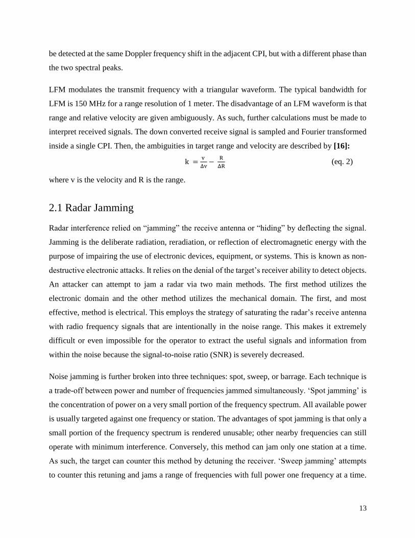
32
Figure 10. Completed Searching Can Radar
This photo, edited with Microsoft Visio, shows the completed
construction of the radar. The top left can is the receiving antenna, and
the other can is the transmitting antenna. Underneath is the mounted
RF chain that is powered by the circuits below. The battery packs are
blacked on the left, which are connected to the circuits. The plexiglass
that the components are mounted to is held up by four cans.
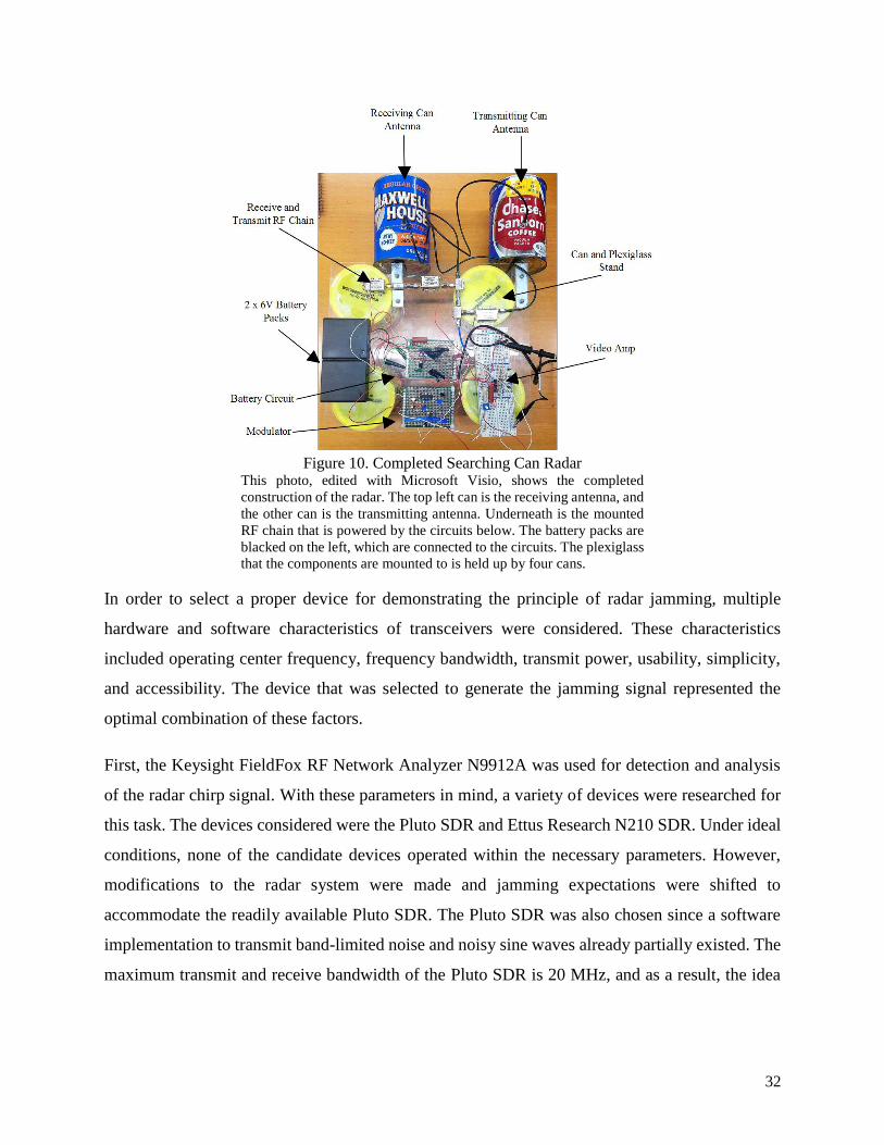
In order to select a proper device for demonstrating the principle of radar jamming, multiple
hardware and software characteristics of transceivers were considered. These characteristics
included operating center frequency, frequency bandwidth, transmit power, usability, simplicity,
and accessibility. The device that was selected to generate the jamming signal represented the
optimal combination of these factors.
First, the Keysight FieldFox RF Network Analyzer N9912A was used for detection and analysis
of the radar chirp signal. With these parameters in mind, a variety of devices were researched for
this task. The devices considered were the Pluto SDR and Ettus Research N210 SDR. Under ideal
conditions, none of the candidate devices operated within the necessary parameters. However,
modifications to the radar system were made and jamming expectations were shifted to
accommodate the readily available Pluto SDR. The Pluto SDR was also chosen since a software
implementation to transmit band-limited noise and noisy sine waves already partially existed. The
maximum transmit and receive bandwidth of the Pluto SDR is 20 MHz, and as a result, the idea

33
of displaying the full spectrum of the radar signal was abandoned. Instead, the SDR would simply
jam the operation of the radar. The Pluto SDR is shown in Figure 11.
Figure 11. Pluto SDR [24] This photo depicting Analog Devices’ Pluto SDR shows the relative
simplicity and compactness of the device. The right antenna is used to
transmit signals, while the left antenna is used to receive signals. The
device utilizes an internal Field-Programmable Gate Array (FPGA),
and is powered through a standard Universal Serial Bus (USB)
connection to a computer or outlet.
Since the radar’s bandwidth is 80 MHz, one Pluto SDR alone could not effectively jam the entire
spectrum of operation because each one only generates enough noise to jam about one quarter of
the operation range. Therefore, two Pluto SDRs were used to jam a majority of the radar signal.
Bandwidth limitations were not the only concern when attempting to jam the radar signal. The
transmit power limitation was the main concern of using one Pluto SDR. This was because the
Pluto has significantly lower transmit power in comparison to the radar. In order to effectively jam
the radar, +19 dB of attenuation was attached to the transmitting antenna of the radar to bring the
radar’s overall power down to a level that was comparable to the transmit power of the Pluto SDR.
This change showed that bandlimited noise at a high enough power could jam a frequency
modulated signal. The figures presented below demonstrate the spectrum measurements that were
taken during testing to determine the relative power and frequency bandwidth of the Pluto SDR
and radar signal. These measurements were taken on the FieldFox.

34
Figure 12. Relative Power Measurement of FMCW Radar Signal This photo depicts the relative power measurement of the FMCW. It
shows that, on average, the radar signal is operating at a power of about
-12 dBm. This approximate value is only valid under the 80 MHz
frequency bandwidth that the signal occupies. Outside of the 80 MHz
bandwidth range, the power levels drop off significantly, since the
FMCW radar is not operating at these frequencies and the spectrum
analyzer is reading the baseline level of -42 dBm.
Figure 13. Frequency Bandwidth Measurement of FMCW Radar This photo depicts the frequency bandwidth measurement of the
FMCW radar waveform. It shows that, on average, the radar signal is
operating at a bandwidth of about 80 MHz Outside of the 80 MHz
bandwidth range, the power levels drop off significantly, since the
FMCW radar is not operating at these frequencies.

35
Figure 14. FMCW Radar Signal vs SDR-generated Noise Power This photo depicts an overlay of the frequency bandwidth of the
FMCW radar waveform with the noisy sinusoidal generated by the
SDR.
Figure 14 shows that, on average, the radar signal is operating at a power level of about -30 to -20
dB. The jamming signal, in comparison, only peaked out at about a power level of -50 dB.
Therefore, the signal did not interfere with the operation of the radar as well as expected in this
first test. It should also be noted that the jamming signal only occupied about ¼ of the 80 MHz
spectrum that the radar occupied. In Figure 15, the band-limited noise, in comparison, only peaked
out at about a power level of -35 dB. Therefore, the signal did not interfere with the operation of
the radar as well as expected, but it was better than the previous test. It should also be noted that
the jamming signal occupied about 1/3 of the 80 MHz spectrum that the radar occupied in this
second test, which was an improvement from the previous test.
Once the Pluto SDR was chosen to jam the radar, the next step was to program the device to
produce a signal that would interfere with the radar operation. Two different approaches were
tested to determine which produced the highest level of interference. The first approach used
sinusoidal waves with a high degree of white Gaussian noise overlaid in an attempt to block the
radar’s ability to detect a person walking. The second approach extended this concept by
generating a band-pass filter and transmitting band-limited white Gaussian noise through the
wideband filter. Both of these approaches are discussed separately below.

36
Figure 15. Band-Limited Noise Signal Interference
This photo depicts an overlay of the frequency bandwidth of the
FMCW radar waveform with the noise signal generated by the SDR.
It shows that, on average, the radar signal is operating at a power level
of about -30 to -20 dB.
To begin, the SDR was set up using default constants in Ubuntu. This included utilizing the
wrapper class that allows the radio to interface with MATLAB properly using the libiio class. Once
the default values were set, the transmit and receive frequencies were changed to approximately
2.438 GHz with a bandwidth of 80 MHz. These values came from the measurements of the radar
signal shown in the previous sections. A sine wave of 100 kHz was generated, and the AWGN
(additive white Gaussian noise) function degraded the sine wave so it was noisy and imprecise to
model a realistic attack on the radar. Different signal-to-noise ratios (SNR) were tested, and
through trial and error, it was determined that an SNR of .01 was noisy enough to impact the
operation of the radar signal. The non-ideal sine wave was run through a for loop containing a
number of iterations equal to the number of frames chosen to transmit.
Both the tic and toc functions were used to approximate the length of time it took for the computer
to transmit a frame of data. A predetermined arbitrary value of twenty frames were transmitted to

37
begin. Eventually, instead of transmitting a predetermined number of frames, an infinite while loop
was generated to keep the radio transmitting the noisy sine waves until the team stopped the
MATLAB function from running by hand. It should be noted that a 100 kHz sine wave was chosen
since the radio’s software generates the wave, and then modulates the signal up from baseband to
RF frequencies. In this scenario, the signal that was transmitted from the SDR was at 2.438 GHz
± 100 kHz. After significant testing, it was determined that a new approach was needed to
effectively jam the signal as the bandwidth of the radar was much larger than that that could be
covered by a single frequency noisy sine wave.
As such, the next approach was to design a wall of noise that could bombard the receiver or
transmitter and block either or both from detecting the motion of any objects. A “wall” of noise is
defined as high power noise signals that occupy a large range of frequencies. It is called a wall
because it simulates the effect of a time-varying signal being absorbed by a wall in a mechanical
sense. In order to generate the bandpass filter required to focus this bandlimited noise between a
range of desired frequencies, the operating limits of the Pluto SDR had to be considered again.
Since the Pluto SDR has a maximum frequency bandwidth of about 20 MHz, the bandpass filter
had to have a range larger than this to ensure that the entire available spectrum would be filled
with noise.
The designfilt function was used to create the unique bandpass filter. A minimum cutoff frequency
of 20 Hz was chosen, with an upper cutoff frequency of 40 MHz. An array of all ones was created,
of length channel size. This decision ensured that the data transmitted would contain as much data
as the SDR could handle. The array was then made non ideal and random by overlaying additive
white Gaussian noise onto each element of the array. This array was then sent through the bandpass
filter designed above. After the filter, the new array was then modulated up to 2.4 GHz and
transmitted over the air using the SDR transceiver function. The figure below demonstrate the
bandpass filter frequency response that was generated, as well as the frames of noisy data that were
transmitted.

38
Figure 16. Magnitude Response of Bandpass Filter This photo depicts the magnitude response of the bandpass filter that
was generated using the designfilt MATLAB Function to focus the
noise signal in the operating range of the radar signal. The lower cutoff
frequency was 20 Hz, and the upper cutoff frequency was 40 MHz.
The filter needed to reject DC, and also reject
4.2 Simulations
Before testing began, simulations were conducted to predict the behavior of the hardware
components and software functions.
The modulator circuit was essential in altering the amplitude and frequency of the oscillator’s
tuning frequency. To ensure the performance of the circuit, it was built and simulated in LTspice.
Simulating the operation of the radar took on the form of utilizing the preexisting MATLAB
model. However, this model was refactored to include upgraded functionality. The upgraded
functionality now accounted for non-idealities in the transmission and reception channel. Non
idealities included the introduction of Additive White Gaussian Noise (AWGN) as well as a
variation of the inverse square law to model signal attenuation over distance.

39
Figure 17. Modulator Circuit in LTspice This schematic was built using the software LTspice. The function
generator chip, XR-2206 was used in this model to provide accurate
simulations. Additionally, each pin output had the same components
and values as the schematic provided by MIT Lincoln Laboratory.
The pins that were closely analyzed were pin 11, Vtune to the oscilloscope, and pin 2, the sync
pulse. Their waveforms are shown below.
Figure 18. Modulator Waveforms These waveforms, generated using LTspice, show the expected square
wave from the sync pulse (blue) and the expected triangle wave from
the Vtune (green).
Another new functionality was the introduction of the ability to create and identify a model of
phase shifts in the system. The signal that was generated was then phase shifted and overlaid on
top of the original signal for comparison. The mean squared error between the original signal and
the phase shifted version was also calculated and plotted to demonstrate the effect of phase shifting
on the system's’ operation. It is important to note that the simulation was run at a low frequency
of 5-50 Hz so that the chirp signal could be visualized graphically. However, the simulation was

40
then re-run at higher frequencies in order to obtain results that would be closer to the actual
operation of the radar and jamming signal at a center frequency of 2.4 GHz. These higher
frequencies included 5-50 kHz, 50-500 kHz, and 500 MHz.
The last simulation required the use of higher computational power than was available to any single
team member via a personal computer. Therefore, the computing power of the Electrical and
Computer Engineering department was utilized through the use of the computer and processors
onboard the Goat Cart Major Qualifying Project. This computer was needed in order to store the
high amount of data required to run the simulation at 500 MHz, as well as process it in a timely
manner. The figures shown below demonstrate the software's functionality at varying minimum
and maximum sweep frequencies.
Figure 19. 5-50 Hz FMCW Chirp with Mean Squared Error
This figure was generated by the MATLAB script that simulates the
signal processing functions of the transmit and receive RF chains of
the radar. This is the baseline frequency and least error.

41
The script produces four different plots each time it is run. The MATLAB script takes a variety of
inputs that are parameters relevant to the operation of the radar, the most notable being the
bandwidth and frequency of operation. The mean squared error was plotted between a simulated
jammed signal and the original chirp signal sent out by the radar. Figure 19 shows a test of the
simulation at a relatively low frequency so that the behavior of the individual wavelengths could
be distinguished with the human eye. Figure 20 shows the simulation at a frequency bandwidth of
5-50 kHz. The wave behavior is no longer intelligible to the human eye, but the increased number
of samples provides a slightly better approximation of the radar operation. Figure 21 shows the
simulation at a frequency bandwidth of 50-500 kHz and again, the graph is unintelligible. The final
simulation required higher computing power; as such the memory and processing power of the
computer onboard the Goat Cart Major Qualifying Project was utilized. This produced the output
found in Figure 22.
Figure 20. 5-50 kHz FMCW Chirp with Mean Squared Error
This figure was again generated by the MATLAB script that simulates
the signal processing functions of the transmit and receive RF chains
of the radar. The error has increased significantly.

42
Figure 21. 50-500 kHz FMCW Chirp with Mean Squared Error This figure was again generated by the MATLAB script that simulates
the signal processing functions of the transmit and receive RF chains
of the radar. The error is indiscernible, but has increased with the
higher frequency.
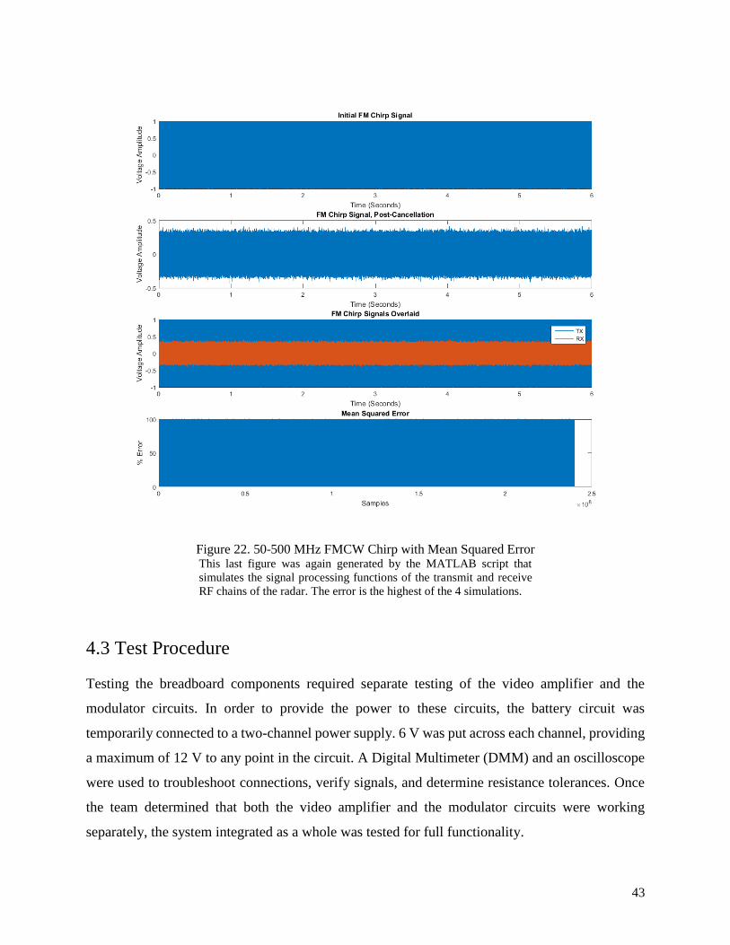
43
Figure 22. 50-500 MHz FMCW Chirp with Mean Squared Error This last figure was again generated by the MATLAB script that
simulates the signal processing functions of the transmit and receive
RF chains of the radar. The error is the highest of the 4 simulations.
4.3 Test Procedure
Testing the breadboard components required separate testing of the video amplifier and the
modulator circuits. In order to provide the power to these circuits, the battery circuit was
temporarily connected to a two-channel power supply. 6 V was put across each channel, providing
a maximum of 12 V to any point in the circuit. A Digital Multimeter (DMM) and an oscilloscope
were used to troubleshoot connections, verify signals, and determine resistance tolerances. Once
the team determined that both the video amplifier and the modulator circuits were working
separately, the system integrated as a whole was tested for full functionality.

44
To begin testing, each power supply channel was set to 6 V with a current limit of approximately
200 mA. After the supplies were connected to the battery circuit, the function generator was set to
produce a 15 kHz sine wave. This was then connected to the input of the video amplifier circuit.
An oscilloscope probe was connected to that input as well as the output to compare the signals. To
verify that the system works correctly, the team check that the video amplifier produced
approximately a -3 dB roll-off at about 15 kHz. Frequencies higher than 15 kHz displayed a steeper
roll-off, which is indicative of proper behavior.
In order to test the modulator circuit, the power supply channels were again set to 6 V each, with
a current limit of 200mA. One probe of the oscilloscope was connected to the output (labeled pin
2 in the schematic) and the other probe should be connected to the ramp generator (pin 4). Upon
adjusting the two potentiometers, the up-ramp time should be 20 ms, and the ramp magnitude
should be 2-3.2 V.
This section details the testing that was done to the can antennas prior to being mounted on the
plexiglass base. The antennas needed to be tuned further than just trimming the metal leads of the
waveguides down to a multiple of λ/4. The antennas required tuning so that the transmitted and
received signals were in the correct frequency band; a spectrum analyzer was used to determine
the general behavior of the antennas before any tuning was attempted. The figures below
demonstrate the resonance behavior of the transmit and receive antennas. The first figure
demonstrates a 50Ω input impedance and reading of about -30 dB constant across a large range of
frequencies.
The reading in Figure 23 was taken before antenna tuning began; it was a calibration test to
determine if the spectrum analyzer was functioning properly. As the magnitude response shows,
the relative constant power across a wide range of frequencies means that the device is reading a
strictly fixed input impedance of 50 Ω correctly.

45
Figure 23. Baseline Calibration Magnitude Response of Spectrum Analyzer with 50 Ω Input
This photo depicts a baseline power reading for a 50 Ω input
impedance. It demonstrates the calibration of the spectrum analyzer
that was performed before tuning of either antenna was attempted. A
50 Ω input impedance is a useful calibration measure because it
represents a proper match of the line with the load. Therefore, the
baseline reading of -30 dB allowed the team to determine the relative
power levels that all measurements should be made with respect to.
Figure 24. Tuning of Transmit Antenna -12 dB Resonance This photo depicts the tuning of the transmit antenna of the radar. It
demonstrates the resonance behavior at a power level of about -12 dB
at a frequency of 2.1876 GHz. This resonance was a little below the
expected frequency value of 2.4 GHz, but still demonstrated the
behavior that was expected of an antenna operating in the correct
frequency band.

46
Figure 25. Tuning of Receive Antenna -20 dB Resonance
This photo depicts the tuning of the receive antenna of the radar. It
demonstrates the resonance behavior at a power level of about -40 dB
at a frequency of 2.41 GHz. This resonance was slightly above the
expected frequency value of 2.4 GHz, but still demonstrated the
behavior that was expected of an antenna operating in the correct
frequency band.
The resonant behavior of both the transmit and receive antennas were not identical for a few
reasons. To begin, the goal of the tuning behavior was twofold. To have the resonance occur at
the highest power level possible, and to occur at the correct frequency (as close to 2.4 GHz as
possible). Although the resonance of each can was fairly close to 2.4 GHz, the power levels were
somewhat different. This could be attributed to non-idealities in the can shape and dimensions. It
could also be attributed to the placement of the antenna inside the can. The holes drilled for the
connections were measured to be as centered as possible, but some human error was incurred
when drilling and inserting the antennas. This resulted in slightly different magnitude responses.
Overall, the can antennas magnitude responses were sufficient over the frequency range of
interest for this application.
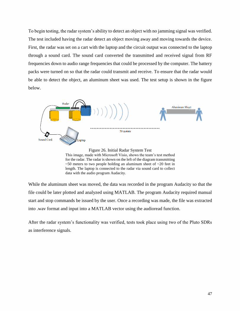
47
To begin testing, the radar system’s ability to detect an object with no jamming signal was verified.
The test included having the radar detect an object moving away and moving towards the device.
First, the radar was set on a cart with the laptop and the circuit output was connected to the laptop
through a sound card. The sound card converted the transmitted and received signal from RF
frequencies down to audio range frequencies that could be processed by the computer. The battery
packs were turned on so that the radar could transmit and receive. To ensure that the radar would
be able to detect the object, an aluminum sheet was used. The test setup is shown in the figure
below.
Figure 26. Initial Radar System Test
This image, made with Microsoft Visio, shows the team’s test method
for the radar. The radar is shown on the left of the diagram transmitting
~50 meters to two people holding an aluminum sheet of ~20 feet in
length. The laptop is connected to the radar via sound card to collect
data with the audio program Audacity.
While the aluminum sheet was moved, the data was recorded in the program Audacity so that the
file could be later plotted and analyzed using MATLAB. The program Audacity required manual
start and stop commands be issued by the user. Once a recording was made, the file was extracted
into .wav format and input into a MATLAB vector using the audioread function.
After the radar system’s functionality was verified, tests took place using two of the Pluto SDRs
as interference signals.

48
Figure 27. Radar System Test with Pluto SDRs This image, made with Microsoft Visio, shows test method for the
radar with the addition of the Pluto SDRs. The SDRs are shown being
powered from the second laptop and being aimed at the antennas of
the radar. The remainder of the setup is the same.
4.4 Chapter Summary
The focuses of this chapter are the methods in which the radar was be built and tested. This includes
the major steps of putting together and testing RF chain, analog components, can antennas, as well
as the MATLAB code. Then, the method for verifying that the system as a whole could function
correctly was explained. Finally, the jamming method using the Pluto SDR was explored. The
following chapter addresses the results that were produced from the above test plans.

49
5 Experimental Results
This section analyzes the experimental results collected from designing, simulating, testing, and
troubleshooting the operation of the radar system and SDR jamming signal.
5.1 Full System Operation
The radar’s functionality was tested in multiple scenarios to determine the maximum operating
range, transmit power, and overall resolution of detection. It was tested on objects with both a low
and high Radar Cross Section (RCS), as well as on objects moving at varying speeds, distances,
and directions. The results of these tests are shown in the plots below. The MATLAB script
read_data_RTL.m receives a .wav audio file, and plots the distance versus time of objects detected
using the Inverse Discrete Fourier Transform or IDFT.
To begin, multiple baseline readings using the radar were taken to determine what a standard range
versus distance plot yielded when there was no distinct jamming signal present to interfere with
the detection of a person away from and towards the radar receiver. The baseline readings were
tested inside the Electrical and Computer Engineering building Atwater Kent (AK) second floor
laboratory and straight hallways, as well as outside on the WPI campus between the fountain area
and Salisbury street. The plots below demonstrate the baseline behavior of the radar.
In Figure 28, the script stores the audio data from the .wav file in an array, and then uses
logarithmic and signal processing mathematics to plot the range versus time plot of objects that
the radar detects. These calculations are completed using the amount of electromagnetic energy
that is reflected off the target and back towards the receiver. This figure depicts the motion of a
person walking away from and then towards the radar receiver over a time length of about 18
seconds. The same scenario is shown in Figure 29 at a time of 25 seconds.

50
Figure 28. Radar Reading of Person Walking in AK227 Test #1 This figure was generated by the MATLAB script that calculates the
Inverse Discrete Fourier Transform (IDFT) of a .wav audio file.
Figure 29. Radar Reading of Person Walking in AK227 Test # 2 This figure was again generated by the MATLAB script that calculates
the Inverse Discrete Fourier Transform (IDFT) of a .wav audio file.

51
Figure 30. Atwater Kent Room 227
As can be seen from the picture above, the radar was tested on a
walkway that was about 15 meters in length. This represented a
controlled environment in which the noise was fairly predictable and
multiple tests produced similar results.
As can be seen from the plots above, testing a movement as simple as walking back and forth can
result in slightly different power outputs from the radar due to varying levels of noise, as well as
the presence of other noisy signals from people’s electronic devices in the room. However, the
same general trend is present in the graphs in these two tests.
Figure 31. Test Between Salisbury Street and WPI Fountain
This figure was generated by the MATLAB script that calculates the
Inverse Discrete Fourier Transform (IDFT) of a .wav audio file.

52
Figure 31 depicts the motion of a person walking towards the radar receiver from Salisbury Street
over a time of 55 seconds. This plot is less precise than when inside the building because the range
was much larger outside and wind interfered with the testing. It can be seen that the radar picks up
the motion of targets to a maximum range of about 70 meters.
Figure 32. WPI Fountain and Walkway towards Salisbury Street [25]
The radar was tested on an outdoor walkway that was about 70 meters
in length. This represented an environment in which the noise was
fairly unpredictable and multiple tests produced varying results.
Figure 33. Walking Test with Metal Sheet
This figure was generated by the MATLAB script that calculates the
Inverse Discrete Fourier Transform (IDFT) of a .wav audio file.

53
Figure 33 depicts the motion of a person walking away from and towards the radar receiver over
a time of 55 seconds. A metal sheet was added to increase the received signal of the radar. This
plot is less precise than when inside the building because the range was much larger outside and
wind and people interfered with the testing. It can be seen that the radar picks up the motion of
targets to a range of about 45 meters in this case. The energy returns were higher in this scenario
since a metal sheet was used.
Figure 34. Walkway In Front of Atwater Kent Laboratories [26] As can be seen from the picture above, the radar was tested on a
walkway that was about 45 meters in length. This represented a
variable environment in which the noise was fairly unpredictable and
multiple tests produced somewhat similar results. Student movement
around the building did interfere with some of the testing.
The two plots shown in Figures 31 and 33 demonstrate the operation of the radar in less ideal
conditions than when the device was tested inside the building. This is evident by the increased
amount of noise and scattered power distributions. However, the distinct trend of an object moving
away from and then towards the receiver is still fairly evident. The noise could be attributed to a
few factors. First, there was significant wind blowing the metal banner that was reflecting the
electromagnetic energy. Therefore, the banner was twisting and turning, and thus changing its RCS
over time. Secondly, there were other people present on the campus during testing, and a few
people walked in front of the receiver during the recording.

54
As discussed in the previous section, multiple Pluto SDRs were used to jam the operation of the
radar. Before the SDR’s were used to jam the signal however, a metal tin was placed in front of
the receiver to simulate a high-powered noise jamming attack or chaff attack on a real radar. The
results of both types of jamming are displayed and discussed below.
The introduction of the metal tin in front of the radar receiver at time instant 11 is fairly clear; the
horizontal line on the graph above that shows relatively stable high power of about 0 dB to -10 dB
is a representation of the radar failing to make accurate distance measurements. It is nearly
impossible for an object with such high power to be present instantaneously ranging from 0-70
meters with no indication of its existence before that time. Therefore, it is safe to assume the radars
receiver and signal processing functions were jammed, causing the IDFT plot to fail. Also, instead
of seeing the characteristic line with positive slope tracking the movement of the person back
towards the receiver, the received power is scattered across a variety of range values, making it
impossible for a radar operator to track the movement of the intended target.
Figure 35. Radar Jammed Using Metal Tin
This figure was generated by the MATLAB script that calculates the
Inverse Discrete Fourier Transform (IDFT) of a .wav audio file.

55
Figure 35 depicts the motion of a person walking away from and towards the radar receiver over
a time of 20 seconds. A metal tin was placed in front of the receiver at time 11, and all readings
after that point are scattered energy returns that are unintelligible.
Figure 36. Radar Jammed Continuously Using Two Pluto SDRs This figure was generated by the MATLAB script that calculates the
Inverse Discrete Fourier Transform (IDFT) of a .wav audio file.
Figure 36 depicts the motion of a person walking away from and towards the radar receiver over
a time length of about 12 seconds. This plot shows slight energy changes but contains no
discernable path to track the movement of a person. Thus, this proves the concept of jamming an
FMCW radar signal.
The introduction of the Pluto SDR’s in front of the radar receiver is fairly clear; the horizontal
lines on the graph above that shows relatively stable high power of about 0 dB to -10 dB are a
representation of the radar failing to make accurate distance measurements. It is nearly impossible
for an object with such high power to be present instantaneously ranging from 0-70 meters with
no indication of its existence before that time. Therefore, it is safe to assume the radars receiver
and signal processing functions were jammed, causing the IDFT plot to fail.

56
5.2 Chapter Summary
The focus of this chapter is the demonstration of the radar’s operation in different scenarios
including inside a laboratory, inside a hallway, and outside a building. The figures presented also
demonstrate the ability of a SDR to jam an FMCW signal. Instead of seeing the characteristic
line with positive and negative slopes tracking the movement of the person walking away from
and towards the receiver, the received power is scattered across a variety of range values. This
makes it impossible for a radar operator to track the movement of the intended target. This is a
demonstration of proof of concept; a FMCW can be jammed with directed band-limited noise.

57
6 Conclusions
In conclusion, this project investigated the design, testing, and jamming of a radar system. The
project served as proof of concept that an analog FMCW radar signal could be jammed using an
SDR. The radar was effectively jammed through the use of a focused noise transmission. The team
learned about the operation of radar, different jamming techniques, multiple system
implementations, and radio frequency measurement tools.
The first and main project objective was successfully met, which was to simulate, build, and test a
radar that can detect an object approximately 50m away. Through the guidelines provided by MIT
Lincoln Labs, the coffee can radar was built so that it could accurately identify an aluminum sheet
held by two people walking back and forth. This was accomplished by ensuring the can antennas
were tuned, building the RF transmit and receive chain, and building the analog circuits, the
modulator and video amplifier, on breadboards. Additionally, the sub-task of jamming the radar
was also successfully completed. By programming two Pluto SDRs to transmit noise, the radar
signal was interfered, thus inhibiting its ability to detect the aluminum sheet. Data from the tests
of both objectives were analyzed in MATLAB using the radar’s audio files that were recorded in
Audacity.
Numerous challenges were presented throughout the course of the project. Primarily, time and
budget constraints became important factors in deciding what objectives could be accomplished.
Because each radar test bed is over $400 to construct, with approximately $200 in additional and
spare parts, having a $1,000 would not allow us to make more than one test bed. Similarly, a time
span of fewer than 3 terms, each of 7 weeks, provided appropriate time for building, testing, and
jamming only one radar.
The results of this project have numerous implications for the present day. Foremost, it exposes a
vulnerability in low incidence radar systems. If the bandwidth and frequency chirp of the radar can
be determined, then the radar can be jammed even with rudimentary electrical attacks such as
bandlimited noise jamming. This is a concern for the automotive industry as many self-driven cars
implement this technology to navigate. This leads to an obvious need for further investigation into

58
how to make these systems more resilient against attack and, in the event of attack, there are
sufficient countermeasures in place.
6.1 Future Work
The research, designs, implementations, and proof of concept demonstrated in this project could
be extended in future work in a variety of different ways. The most significant would be designing
a different radar to jam that utilizes some other medium besides coffee cans as the antennas and
waveguides. This would allow for less signal attenuation and more predictable radio frequency
behavior. In line with the idea of redesigning subsections of the system, a transmitter or SDR with
higher transmit power could also be a potential option that would allow for more accurate results
and readings of the jamming concept. In this manner, only one device would be required to jam
the radar, and no extra attenuation would need to be introduced at the receiver of the radar to make
the power ratios closer together.
A second extension of this project might involve changing the focus of the project to demonstrate
the concept of analog phase cancellation in the time domain. This would essentially demonstrate
the jamming of a FMCW radar signal through the use of a replay attack. The system architecture
would contain one radar attempting to detect objects, and another radar that latches onto the radar
signal and replays a phase-shifted version back at the receiver of the radar to disable the ability to
detect objects nearby. The noise jamming conducted in the team’s current design would be a
precursor to this design.

59
Appendices
Appendix A: Cost of Materials
Name Qty Description Supplier Cost/Unit Total Cost
solderless breadboard 2 6.5x1.75" Amazon $6.94 $13.88
Video Amp1 2 low-noise quad opamp Digi-Key $6.36 $12.72
C1-4 8 1000 pf 5% Digi-Key $0.39 $3.12
R1a_1 2 8450 ohm 1% Digi-Key $0.10 $0.20
R1b_1 2 102K ohm 1% Digi-Key $0.10 $0.20
R2_1 2 7150 ohm 1% Digi-Key $0.10 $0.20
Rf_1_2 3 1K ohm 1% Digi-Key $0.10 $0.30
Rg_1 6 12.1K ohm 1% Digi-Key $0.10 $0.60
R1a_2 2 17.4K ohm 1% Digi-Key $0.10 $0.20
R1b_2 2 28K ohm 1% Digi-Key $0.10 $0.20
R2_2 2 4120 ohm 1% Digi-Key $0.10 $0.20
Rg_2 2 1620 ohm 1% Digi-Key $0.10 $0.20
5V regulator 2 5V low dropout regulator Digi-Key $1.55 $3.10
100k resistor 10 100k resistor Digi-Key $0.10 $1.00
1uf capacitor unpolarized 2 1 uf film capacitor Digi-key $0.97 $1.94
Wire ties 2 4" cable ties Home Depot $4.99 $9.98
Modulator1 2 Function Generator Chip Jameco $7.95 $15.90
Battery pack 4 4xAA battery pack with power
switch Jameco $2.49 $9.96
L bracket 4 L bracket McMaster
Carr $0.43 $1.72
6-32 screws 2 6-32 screws McMaster
Carr $3.49 $6.98
6-32 nuts 2 6-32 nuts McMaster
Carr $1.24 $2.48
6-32 lockwashers 2 6-32 lockwashers McMaster
Carr $0.62 $1.24
Wood Screws 2 screws 3/8" long, pk 100 McMaster
Carr $4.90 $9.80

60
OSC1 2 VCO Mini-Circuits $44.95 $89.90
ATT1 2 Attenuator Mini-Circuits $13.95 $27.90
PA1/LNA1 5 LNA Mini-Circuits $39.95 $199.75
SPLTR1 2 Splitter/Combiner Mini-Circuits $34.95 $69.90
MXR1 2 Mixer Mini-Circuits $46.45 $92.90
SMA M-M 8 Adapter Mini-Circuits $5.95 $47.60
6" SMA M-M cables 6 6" SMA M-M cables Mini-Circuits $9.75 $58.50
SMA F bulkhead 4 SMA F bulkhead Mouser $6.12 $24.48
Decoupling Cap 4 0.1 uf Mouser $0.29 $1.16
Decoupling Cap2 4 100 uf Mouser $0.30 $1.20
trimmer potentiometer 2 10k Mouser $1.43 $2.86
gain resistor 2 200 ohm, 5% Mouser $0.33 $0.66
Audio Cord 2 3.5 mm plug to stripped wires Mouser $3.63 $7.26
Turning capacitor 2 0.47 uf 250V Rated Mouser $1.69 $3.38
2m trimmer potentiometer 2 2m trimmer potentiometer Mouser $1.52 $3.04
50k trimmer potentiometer 2 50k trimmer potentiometer Mouser $1.52 $3.04
1uf cap 2 1 uF electrolytic cap M Mouser $0.24 $0.48
10uf cap 4 10 uF electrolytic cap Mouser $0.31 $1.24
5.1k resistor 4 5.1k resistor Mouser $0.12 $0.48
10k resistor 4 10k resistor Mouser $0.10 $0.40
LED 2 Red Mouser $0.42 $0.84
1K LED resistor 2 1K LED resistor Mouser $0.10 $0.20
47k resistor 24 47K 5% resistor Mouser $0.92 $22.08
Can 4 Cans Donation $0 $0
AA batteries 2 AA batteries Target $10.29 $20.58
TOTAL $762.07

61
Appendix B: MATLAB Code
model.m %% Initialize the model parameters
clearvars; close all; clc
% Chirp settings
chirp_fmin = 5; % Hz
chirp_fmax = 50; % Hz
chirp_fs = 10*chirp_fmax; % Hz
chirp_amplitude = 1; % volts
chirp_duration = 3; % seconds
% Signal settings
num_chirps = 2;
total_duration = chirp_duration * num_chirps; % seconds
TX_power = 10; % mW
% Channel settings
distance_to_target = 30; % meters
channel_snr = 10; %dB
%% Create the initial chirp
% Out: signal_init
% Create a time vector for a single chirp
num_chirp_time_samples = chirp_fs * chirp_duration;
chirp_time_vector = linspace(0, chirp_duration, num_chirp_time_samples);
% Create one chirp vector
single_chirp = chirp( ...
chirp_time_vector, chirp_fmin, chirp_time_vector(end), chirp_fmax);
% Create a time vector for the entire, multi-chirp signal
num_total_time_samples = chirp_fs * total_duration;
total_time_vector = linspace(0, total_duration, num_total_time_samples);
% Create a multiple chirp vector
signal_init = repmat(single_chirp, 1, num_chirps);
%% TX Attenuation (-3dB ATT1)
% In: signal_init
% Out: signal_TXatt
tx_attenuation = -3; % dB
scaling_factor = 10^(tx_attenuation/10);
signal_TXatt = scaling_factor * signal_init;
%% TX Amplification (+14dB PA1)
% In: signal_TXatt
% Out: signal_TXamp
tx_amplification = 14; % dB
scaling_factor = 10^(tx_amplification/10);
signal_TXamp = scaling_factor * signal_TXatt;

62
%% TX Splitter (+11dB SPLTR1)
% In: signal_TXamp
% Out: signal_TXsplit
tx_splitter_amp = 11; % dB
scaling_factor = 10^(tx_splitter_amp/10);
signal_TXsplit = scaling_factor * signal_TXamp;
%% Channel Non-idealities (AWGN, distance attenuation)
% In: signal_TXsplit
% Out: signal_channel
% AWGN
signal_awgn = awgn(signal_TXsplit, channel_snr);
% Distance attenuation
dist_att_factor = sqrt(2)*1/(4*pi*distance_to_target^2);
signal_channel = dist_att_factor * signal_awgn;
%% RX Amplification (+14dB LNA1)
% In: signal_channel
% Out: signal_RXamp
rx_amplification = 28; % dB
scaling_factor = 10^(rx_amplification/10);
signal_RXamp = scaling_factor * signal_channel;
%% Calculate Phase Cancellation
% In: signal_RXamp
% Out: signal_invertedphase
signal_invertedphase = -signal_RXamp;
%% TX2 Attenuation (-3dB ATT1)
% In: signal_invertedphase
% Out: signal_TX2att
tx_attenuation = -3; % dB
scaling_factor = 10^(tx_attenuation/10);
signal_TX2att = scaling_factor * signal_init;
%% TX2 Amplification (+14dB PA1)
% In: signal_TX2att
% Out: signal_TX2amp
tx_amplification = 14; % dB
scaling_factor = 10^(tx_amplification/10);
signal_TX2amp = scaling_factor * signal_TX2att;
%% TX2 Splitter (+11dB SPLTR1)
% In: signal_TX2amp
% Out: signal_TX2split
tx_splitter_amp = 11; % dB
scaling_factor = 10^(tx_splitter_amp/10);
signal_TX2split = scaling_factor * signal_TX2amp;

63
%% Channel Non-idealities (AWGN, distance attenuation)
% In: signal_TX2split
% Out: signal_channel2
% AWGN
signal_awgn2 = awgn(signal_TX2split, channel_snr);
% Distance attenuation
dist_att_factor = sqrt(2)*1/(4*pi*distance_to_target^2);
signal_channel2 = dist_att_factor * signal_awgn2;
%% RX2 Amplification (+14dB LNA1)
% In: signal_channel2
% Out: signal_RX2amp
rx_amplification = 16.5; % dB
scaling_factor = 10^(rx_amplification/10);
signal_RX2amp = scaling_factor * signal_channel2;
%% Perform the final phase cancellation
signal_cancelled = awgn(signal_init - signal_RX2amp, 25);
%% Display results graphically
subplot(4,1,1);
plot(total_time_vector, signal_init);
% Plot 1 - Initial Signal
xlabel('Time (Seconds)');
ylabel('Voltage Amplitude');
title('Initial FM Chirp Signal');
axis([0 6 -1 inf]);
% Plot 2 - Cancelled Signal
subplot(4,1,2);
plot(total_time_vector, signal_cancelled);
xlabel('Time (Seconds)');
ylabel('Voltage Amplitude');
title('FM Chirp Signal, Post-Cancellation');
% Plot 3 - Signal Overlays
subplot(4,1,3);
plot(total_time_vector, signal_init);
hold on;
plot(total_time_vector, signal_cancelled);
xlabel('Time (Seconds)');
ylabel('Voltage Amplitude');
title('FM Chirp Signals Overlaid');
legend('TX','RX')
%% Calculate & Plot Mean-Squared Error (MSE)
MSE = zeros(size(signal_init)); % blank vector to fill
estimate = signal_cancelled; % reassign values
original = signal_init;

64
% MSE calculation & fill vector
for i=1:length(signal_init)
MSE(i) = 100*(sum(((estimate(i) - original(i)).^2)));
end
% Plot Error
subplot(4,1,4);
plot(1:length(MSE),MSE);
ylim([0 100]);
xlabel('Samples');
ylabel('% Error');
title('Mean Squared Error');
radar_jamming.m %% Jam Radar with SDR Tx
clear all; clearvars; close all;
addpath(genpath('../drivers'));
%% createRadio
% % Public, non-tunable properties.
% sdr = PlutoSDR;
% %mode Transceiver mode of SDR
ch_size = 2.^20;
Fs = 30.72e6;
% %in_ch_size Input data channel size [samples]
% sdr.in_ch_size = ch_size;
% %out_ch_size Output data channel size [samples]
% sdr.out_ch_size = ch_size;
% %rx_center_freq Center frequency of RX chain(s) [Hz]
% sdr.rx_center_freq = 2.4e9; % RX_LO_FREQ
% %rx_sample_rate Sample rate of RX chain(s) [Hz]
% sdr.rx_sample_rate = Fs; % RX_SAMPLING_FREQ
% %rx_rf_bandwidth Bandwidth of receive filter [Hz]
% sdr.rx_rf_bandwidth = 5e6; % RX_RF_BANDWIDTH
% %rx_gain_mode AGC mode
% sdr.rx_gain_mode = 'manual'; % RX_GAIN_MODE
% %rx_gain Gain of RX chain(s) [dB]
% sdr.rx_gain = 15; % RX_GAIN
% %tx_center_freq Center frequency of TX chain(s) [Hz]
% sdr.tx_center_freq = 2.438e9; % TX_LO_FREQ
% %tx_sample_rate Sample rate of TX chain(s) [Hz]
% sdr.tx_sample_rate = Fs; % TX_SAMPLING_FREQ
% %tx_rf_bandwidth Bandwidth of transmit filter [Hz]
% sdr.tx_rf_bandwidth = Fs; % TX_RF_BANDWIDTH
%
% sdr.mode = 'transmit';
%% Generate Noisy Sine Wave
Fsine = 1e3;
t = 1/Fs:1/Fs:ch_size/Fs;
amplitude = 4096*8;
frames = 120;
data = ones(1,ch_size);
%data = sin(2*pi*Fsine*t + pi/2);
dataOut = amplitude.*awgn(data, .001);
%% Generate Filter Coefficients

65
bpFilt = designfilt('bandpassfir','FilterOrder',100, ...
'CutoffFrequency1',40,'CutoffFrequency2',40E6, ...
'SampleRate',100E6);
fvtool(bpFilt)
%dataIn = dataOut;
%dataOutFinal = filter(bpFilt,dataIn);
%% Transmit Data
tic
%sdr.transmit(dataOutFinal);
%while(true)
% Tx_data = dataOutFinal;
% sdr.transmit(Tx_data);
% Output Info
%s = strcat({'Frame '}, int2str(frame), {' of '}, int2str(frames));
%disp(s)
%end
toc
%clear sdr;
%figure(2)
%plot(t, Tx_data);
loop_back.m %% Example Loopback
clear all;
addpath(genpath('../drivers'));
%% Setup PlutoSDR
sdr = PlutoSDR;
sdr.mode = 'transceive';
sdr.rx_gain = 10;
sdr.rx_gain_mode = 'fast-attack';
sdr.tx_center_freq = 2.4e9;
sdr.rx_center_freq = 2.4e9;
%% Setup SDR buffers
ch_size = 1e6;
sdr.in_ch_size = ch_size;
sdr.out_ch_size = ch_size;
%% Generate complex transmit signal
Fs = 30.72e6;
Fc = 2.4e9;
t = 1/Fs:1/Fs:ch_size/Fs;
amplitude = 4096;
sigR = sin(2*pi*Fc*t).*amplitude;
sigC = sin(2*pi*Fc*t+pi/2).*amplitude;
sig = complex(sigR,sigC);
%sig = awgn(sigR,30);
%% Transceive with SDR
frames = 20;
cap = zeros(ch_size*frames,1);
prev = 0;
for frame = 1:frames
% Call radio
o = sdr.transceive(sig);
66
% Save data
indx = (frame-1)*ch_size+1 : frame*ch_size;
cap(indx) = o;
% Info
s = sprintf('Frame %d of %d',frame,frames);
fprintf(repmat('\b',1,prev));fprintf(s);prev = length(s);
end
fprintf('\n');
%% Plot
t = 1/Fs:1/Fs:frames*ch_size/Fs;
plot(t,real(cap),t,imag(cap));
xlabel('Sample');
ylabel('Amplitude');
xlim([t(end-300) t(end)])
read_data_RTI.m %MIT IAP Radar Course 2011
%Resource: Build a Small Radar System Capable of Sensing Range, Doppler,
%and Synthetic Aperture Radar Imaging
%Written by: Gregory L. Charvat
%Updated by Michael J. Inserra
%Process Range vs. Time Intensity (RTI) plot
%NOTE: set up-ramp sweep from 2-3.2V to stay within ISM band
%change fstart and fstop below when in ISM band
clear all;
close all;
%read the raw data .wave file here
[Y,FS] = audioread('filename.wav'); %insert .wav file name here
%constant definition
c = 3E8; %(m/s) speed of light
%radar parameters
Tp = 20E-3; %(s) pulse time
N = Tp*FS; %# of samples per pulse
fstart = 2.4E9; %(Hz) LFM start frequency
fstop = 2.48E9; %(Hz) LFM stop frequency
%fstart = 2402E6; %(Hz) LFM start frequency for ISM band
%fstop = 2495E6; %(Hz) LFM stop frequency for ISM band
BW = fstop-fstart; %(Hz) transmit bandwidth
f = linspace(fstart, fstop, N/2); %instantaneous transmit frequency
%range resolution
rr = c/(2*BW);
max_range = rr*N/2;
%the input appears to be inverted
trig = -1*Y(:,1);
s = -1*Y(:,2);
clear Y;
%parse the data here by triggering off rising edge of sync pulse

67
count = 0;
thresh = 0;
start = (trig > thresh);
for ii = 100:(size(start,1)-N)
if start(ii) == 1 & mean(start(ii-11:ii-1)) == 0
%start2(ii) = 1;
count = count + 1;
sif(count,:) = s(ii:ii+N-1);
time(count) = ii*1/FS;
end
end
%subtract the average
ave = mean(sif,1);
for ii = 1:size(sif,1);
sif(ii,:) = sif(ii,:) - ave;
end
zpad = 8*N/2;
%RTI plot
figure(1);
v = dbv(ifft(sif,zpad,2));
S = v(:,1:size(v,2)/2);
m = max(max(v));
imagesc(linspace(0,max_range,zpad),time,S-m,[-80, 0]);
colorbar;
ylabel('time (s)');
xlabel('range (m)');
title('RTI Minimal Clutter Rejection');
%2 pulse cancelor RTI plot
figure(2);
sif2 = sif(2:size(sif,1),:)-sif(1:size(sif,1)-1,:);
v = ifft(sif2,zpad,2);
S=v;
R = linspace(0,max_range,zpad);
for ii = 1:size(S,1)
%S(ii,:) = S(ii,:).*R.^(3/2); %Optional: magnitude scale to range
end
S = dbv(S(:,1:size(v,2)/2));
m = max(max(S));
imagesc(R,time,S-m,[-80, 0]);
colorbar;
ylabel('time (s)');
xlabel('range (m)');
title('RTI With 2-pulse Clutter Rejection');

68
References
[1] J. C. Maxwell, "A Dynamical Theory of the Electromagnetic Field," in wikimedia.org, 1864.
[Online].Available:https://upload.wikimedia.org/wikipedia/commons/1/19/A_Dynamical_Theor
y_of_the_Electromagnetic_Field.pdf. Accessed: Nov. 29, 2016.
[2] V. Jones, "Hertz’s experiments (1887)," in http://people.seas.harvard.edu/. [Online].
Available:http://people.seas.harvard.edu/~jones/cscie129/nu_lectures/lecture6/hertz/Hertz_exp.ht
ml. Accessed: Nov. 29, 2016.
[3] J. Ender, "Hulsmeyer Memorial Speech in the Town Hall of Cologne," in design-
technology.info, 2002. [Online]. Available: http://www.design-
technology.info/resourcedocuments/Huelsmeyer_EUSAR2002_english.pdf. Accessed: Nov. 29,
2016.
[4] G. L. Peterson, "Nikola Tesla--A man of comprehensive solutions," in teslascience.org, 2005.
[Online]. Available: http://www.teslascience.org/pages/tesla.htm#radar. Accessed: Dec. 9, 2016.
[5] M. A. Lorell, J. F. Lowell, M. Kennedy, and H. P. Levaux, "Commercial Technology Trends
Relevant to Military Radars," in Cheaper, Better, Faster? Commercial Approaches to Weapons
Acquisition. Santa Monica, CA: The RAND Corporation, pp. 45–55. [Online]. Available:
https://www.rand.org/content/dam/rand/pubs/monograph_reports/MR1147/MR1147.chap3.final.
pdf. Accessed: Nov. 29, 2016.
[6] J. Rosevear, "Why Volvo and Autoliv are teaming up on self-driving cars," in
www.fool.com/investing, The Motley Fool, 2016. [Online]. Available:
http://www.fool.com/investing/2016/09/06/why-volvo-and-autoliv-are-teaming-up-on-self-
drivi.aspx. Accessed: Dec. 6, 2016.
[7] R. M. O’Donnell, "Introduction to Radar Systems," in www.ll.mit.edu, 2002. [Online].
Available:http://www.ll.mit.edu/workshops/education/videocourses/introradar/lecture1/lecture.p
df. Accessed: Sep. 20, 2016.
[8] "Electronic Warfare and Radar Systems Engineering Handbook," in www.navair.navy.mil,
2013. [Online]. Available:
http://www.navair.navy.mil/nawcwd/ewssa/downloads/NAWCWD%20TP%208347.pdf.
Accessed: Nov. 29, 2016.
[9] Gregory Charvat, Jonathan Williams, Alan Fenn, Steve Kogon, and Jeffrey Herd. RES.LL-
003 Build a Small Radar System Capable of Sensing Range, Doppler, and Synthetic Aperture

69
Radar Imaging. January IAP 2011. Massachusetts Institute of Technology: MIT
OpenCourseWare, https://ocw.mit.edu. License: Creative Commons BY-NC-SA.
[10] B. Vlasic and N. E. Boudette, "Self-driving Tesla was involved in fatal crash, U.S. Says," in
Business Day, The New York Times, 2016. [Online]. Available:
http://www.nytimes.com/2016/07/01/business/self-driving-tesla-fatal-crash-
investigation.html?_r=0. Accessed: Dec. 6, 2016.
[11] D. Jenn, “Radar Fundamentals,” in www.faculty.nps.edu, n.d. [Online]. Available:
http://faculty.nps.edu/jenn/Seminars/RadarFundamentals.pdf. Accessed: Oct. 1, 2016.
[12] A. Fenn, "Antenna Design for the Laptop Radar Project", MIT Lincoln Laboratory, 2011.
[13] C. Wolff, “Radar Principle,” in www.radartutorial.eu, n.d. [Online]. Available:
http://www.radartutorial.eu/01.basics/Radar%20Principle.en.html. Accessed: Oct. 2, 2016
[14] L. Varshney, "Radar System Components and System Design", Syracuse Research
Corporation, North Syracuse, NY, 2002.
[15] D. Bursky, "Low-Noise Amplifiers Maximize Receiver Sensitivity", Digikey.com, 2012.
[Online]. Available: http://www.digikey.com/en/articles/techzone/2012/jun/low-noise-
amplifiers-maximize-receiver-sensitivity. Accessed: Oct. 2, 2016.
[16] G. Kregoski, “FMCW Radar in Automotive Applications: Technology Overview &
Testing,” in www.cst.com. [Online]. Available: https://www.cst.com/~/media/CST/Landing-
Pages/2016automotive/Understanding--Testing-FMCW-Automotive-Radar-Devices.ashx?la=en
[17] H. Rohling and M. Meinecke, "Waveform Design Principles for Automotive Radar
Systems", Technical University of Hamburg, Hamburg, Germany.
[18] Powerpoint Presentation, Topic: "Electronic Attack Tasking”, Federation of American
Scientists. [Online]. Available: https://fas.org/irp/doddir/army/ioac/eaes.htm
[19] Lecturer R.S. Adve, Class Lecture, Topic: "Receive Diversity”, Associate Professor,
University of Toronto, Toronto, Ontario. [Online]. Available:
http://www.comm.utoronto.ca/~rsadve/Notes/DiversityReceive.pdf
[20] D. Bursky, "Low-Noise Amplifiers Maximize Receiver Sensitivity", Digikey.com, 2012.
[Online]. Available: http://www.digikey.com/en/articles/techzone/2012/jun/low-noise-
amplifiers-maximize-receiver-s ensitivity. Accessed: Oct. 2, 2016.

70
[21] H. Chen, 'FMCW radar jamming techniques and analysis', Naval Postgraduate School,
2013. [Online] Available:
http://calhoun.nps.edu/bitstream/handle/10945/37597/13Sep_Chen_HungRuei.pdf?sequence=1
[22] P. E. Pace, Detecting and Classifying Low Probability of Intercept Radar. Norwood, MA:
Artech House, 2009, p. 115-116.
[23] M. A. Aleem, B. Fath, S. H. Gaboury, and F. G. Technologies, Patent US20140111370 -
Bumper Integrated Forward Radar Mounting System. Google Scholar, 2012. [Online]. Available:
https://www.google.com/patents/US20140111370. Accessed: Dec. 10, 2016.
[24] R. Getz, "ADALM-PLUTO: A New $149 TX Capable SDR with 325 - 3800 MHz Range,
12-Bit ADC and 20 MHz Bandwidth - rtl-sdr.com", rtl-sdr.com, 2017. [Online]. Available:
http://www.rtl-sdr.com/adalm-pluto-new-149-tx-capable-sdr-325-3800-mhz-range-12-bit-adc-
20-mhz-bandwidth/. [Accessed: 14-Mar-2017].
[25] V. D'Aquila, "WPI Fountain", Flickr, 2006. [Online]. Available:
https://www.flickr.com/photos/tehchix0r/271454268. [Accessed: 14- Mar-2017].
[26] C. Grosvenor Jr., "Worcester, Mass - Places of the Present, WPI", Worcestermass.com,
1998. [Online]. Available: http://www.worcestermass.com/present/wpi.shtml. [Accessed: 07-
Mar-2017].
[27] D. Pu and A.M. Wyglinski, Digital Communications Engineering with Software Defined
Radio, 1st edition, Artech House, 2013, ISBN-13: 978-1-60807-525-7.
[28] R. Ludwig, G. Bogdanov, RF Circuit Design: Theory and Practice, 2nd edition, Prentice
Hall, 2008, ISBN-13: 9780131471375.