Embed Size (px)
Citation preview

CODE_BRIGHT
2 21 USER’S GUIDE
CODE_BRIGHT 2021 User’s Guide
Edited by Sebastia Olivella, Jean Vaunat and Alfonso Rodriguez-Dono in September 2021
https://deca.upc.edu/en/projects/code_bright

2
TABLE OF CONTENTS
I. CODE_BRIGHT. FOREWORD
I. 1. Introduction
I. 2. System basics
I. 3. Using this manual
II. CODE_BRIGHT. PRE-PROCESS. PROBLEM DATA.
II. 1. Problem type
II. 2. CODE_BRIGHT interface
II. 2.1. Problem data
II. 2.2. Materials
II. 2.3. Conditions
II. 2.4. Intervals data
III. CODE_BRIGHT. PROCESS.
III. 1. Calculate
III. 2. Data Files
III. 3. General information file ROOT_GEN.DAT
III. 4. Geometrical description file ROOT_GRI.DAT
III. 5. Summary-list of cards
IV. CODE_BRIGHT. POSTPROCESS.
IV. 1. Facilities description
IV. 2. Read Post-processing
IV. 3. Post process files format
V. CODE_BRIGHT. THEORETICAL ASPECTS
V. 1. Basic formulation features
V. 2. Governing equations
V. 2.1 Balance equations
V. 2.2 Constitutive equations and restrictions
V. 2.3 Boundary conditions
V. 2.4 Summary of governing equations
V. 3. Numerical Approach
V. 3.1 Introduction
V. 3.2 Treatment of different terms
V. 4. Theoretical approach summary
V. 5. Features of CODE_BRIGHT
V. 6. Parallel version of CODE_BRIGHT
V. 6.1 Matrix storage mode in CODE_BRIGHT
V. 6.2 Iterative solver for nonsymmetrical linear systems of
equations
V. 6.3 Parallel version of CODE_BRIGHT
V. 7. Appendix 1. Thermo-hydro-mechanical interactions

3
VI. CODE_BRIGHT. CONSTITUTIVE LAWS
VI. a. Hydraulic and thermal constitutive laws. Phase properties
VI. b. Mechanical constitutive laws: Elastic and visco-plastic models
VI. c. Mechanical constitutive laws: Damage-Elastoplastic model for
argillaceous rocks
VI. d. Mechanical constitutive laws: Thermo-elastoplastic model
VI. e. Mechanical constitutive laws: Barcelona Expansive model
VI. f. Mechanical constitutive laws: CASM’s family models
VI. g. Excavation/construction process
VI. h. THM discontinuities
CODE_BRIGHT. REFERENCES
___________________________________

4
I. CODE_BRIGHT. FOREWORD
I.1. INTRODUCTION
The program described here is a tool designed to handle coupled problems in geological media.
The computer code, originally, was developed on the basis of a new general theory for saline
media. Then the program has been generalised for modelling thermo-hydro-mechanical (THM)
processes in a coupled way in geological media. Basically, the code couples mechanical,
hydraulic and thermal problems in geological media.
The theoretical approach consists in a set of governing equations, a set of constitutive laws and
a special computational approach. The code is written in FORTRAN and it is composed by
several subroutines. The program does not use external libraries.
CODE_BRIGHT uses GiD system for preprocessing and post-processing. GiD is developed by
the International Center for Numerical Methods in Engineering (CIMNE). GiD is an interactive
graphical user interface that is used for the definition, preparation and visualisation of all the
data related to numerical simulations. This data includes the definition of the geometry,
materials, conditions, solution information and other parameters. The program can also
generate the finite element mesh and write the information for a numerical simulation program
in its adequate format for CODE_BRIGHT. It is also possible to run the numerical simulation
directly from the system and to visualize the resulting information without transfer of files.
For geometry definition, the program works quite like a CAD (Computer Aided Design)
system. The most important difference is that the geometry is developed in a hierarchical mode.
This means that an entity of higher level (e.g. a volume) is constructed over entities of lower
level (e.g. a surface); two adjacent entities (e.g. two volumes) will then share the same lower
level entity (e.g. a surface).
All materials, conditions and solution parameters can also be defined on the geometry without
the user having any knowledge of the mesh. The meshing is performed once the problem has
been fully defined. The advantages of doing this are that, using associative data structures,
modifications can be made on the geometry and all other information will be updated
automatically.
Full graphic visualisation of the geometry, mesh and conditions is available for comprehensive
checking of the model before the analysis run is started. More comprehensive graphic
visualisation features are provided to evaluate the solution results after the analysis has been
performed. This post-processing user interface is also customisable depending on the analysis
type and the results provided.
A query window appears for some confirmations or selections. This feature is also extended to
the end of a session, when the system prompts the user to save the changes, even when the
normal ending has been superseded by closing the main window from the Window Manager,
or in most cases with incorrect exits.
I.2. SYSTEM BASICS
GiD is a geometrical system in the sense that, having defined the geometry, all the attributes
and conditions (i.e., material assignments, loading, conditions, etc.) are applied to the geometry
without any reference or knowledge of a mesh. Only once everything is defined, should the
meshing of the geometrical domain be carried out. This methodology facilitates alterations to
5
the geometry while maintaining the attributes and conditions definitions. Alterations to the
attributes or conditions can simultaneously be made without the need of reassigning to the
geometry. New meshes or small modifications on the obtained mesh can also be generated if
necessary and all the information will be automatically assigned correctly.
The system does provide the option for defining attributes and conditions directly on the mesh
once this has been generated. However, if the mesh is regenerated, it is not possible to maintain
these definitions and therefore all attributes and conditions must be redefined. In general, the
complete solution process can be described as:
1. Define geometry - points, lines, surfaces, volumes.
Use other facilities.
Import from CAD.
2. Define attributes and conditions.
3. Generate mesh.
4. Carry out simulation.
5. View results.
Depending upon the results in step (5) it may be necessary to return to one of the steps (1), (2)
or (3) to make alterations and rerun the simulations.
Building a geometrical domain in GiD is based on the 4 geometrical levels of entities: points,
lines, surfaces and volumes. Entities of higher level are constructed over entities of lower level;
two adjacent entities can therefore share the same level entity.
All domains are considered in 3-dimensional space but if there is no variation in the third
coordinate (into the screen) the geometry is assumed to be 2-dimensional for analysis and
results visualisation purposes. Thus, to build a geometry, the user must first define points, join
these to form lines, create closed surfaces from the lines and define closed volumes from the
surfaces. Many other facilities are available for creating the geometrical domain; these include:
copying, moving, automatic surface creation, etc.
The geometrical domain can be created in a series of layers where each one is a separate part
of the geometry. Any geometrical entity (points, lines, surfaces or volumes) can belong to a
particular layer. It is then possible to view and manipulate some layers and not others. The main
purpose of the use of layers is to offer a visualisation and selection tool, but they are not used
in the analysis.
The system has the option of importing a geometry or mesh that has been created by a CAD
program outside GiD; at present, this can be done via a DXF, IGES or NASTRAN interface.
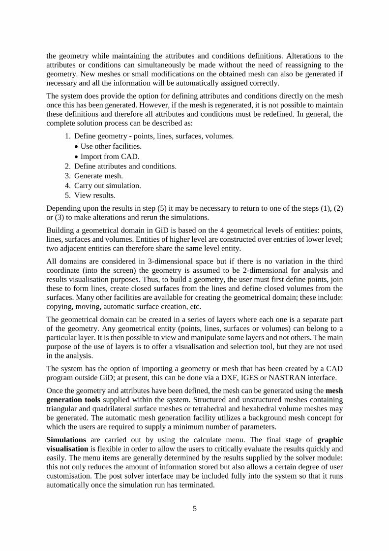
Once the geometry and attributes have been defined, the mesh can be generated using the mesh
generation tools supplied within the system. Structured and unstructured meshes containing
triangular and quadrilateral surface meshes or tetrahedral and hexahedral volume meshes may
be generated. The automatic mesh generation facility utilizes a background mesh concept for
which the users are required to supply a minimum number of parameters.
Simulations are carried out by using the calculate menu. The final stage of graphic
visualisation is flexible in order to allow the users to critically evaluate the results quickly and
easily. The menu items are generally determined by the results supplied by the solver module:
this not only reduces the amount of information stored but also allows a certain degree of user
customisation. The post solver interface may be included fully into the system so that it runs
automatically once the simulation run has terminated.

6
I.3. USING THIS MANUAL
This User Manual has been split into several differentiated parts. The part, THEORETICAL
ASPECTS, contains the theoretical basis of CODE_BRIGHT, and the numerical solution. In
CODE_BRIGHT. PREPROCESS. PROBLEM DATA, it is described how to enter the data
of the problem, i. e. general data, constitutive laws, boundary conditions, initial conditions and
interval data. The referred as CODE_BRIGHT. PROCESS is related to the calculation
process. This part also contains the description of input files. The part, CODE_BRIGHT.
CONSTITUTIVE LAWS contains a description of hydraulic, thermal and mechanical
constitutive laws and phase properties. Finally, CODE_BRIGHT. TUTORIAL, introduces
guided examples for a fast and easy familiarization with the system.
___________________________________
7
II. CODE_BRIGHT. PRE-PROCESS. PROBLEM DATA.
Problem data include all the parameters, conditions (see section Conditions), materials
properties (see section Materials), problem data (see section Problem Data) and intervals data
(see section Interval Data) that define the project. Conditions and materials should be assigned
to geometrical entities.
II.1. PROBLEM TYPE
This option permits to select among all available problem types. When selecting a new problem
type, all information about materials, conditions and other that has already been selected or
defined will be lost. Select CODE_BRIGHT. If an existing project has been created with an old
version of CODE_BRIGHT, use the option Transform to new problem type and
data will be converted to update problem type.
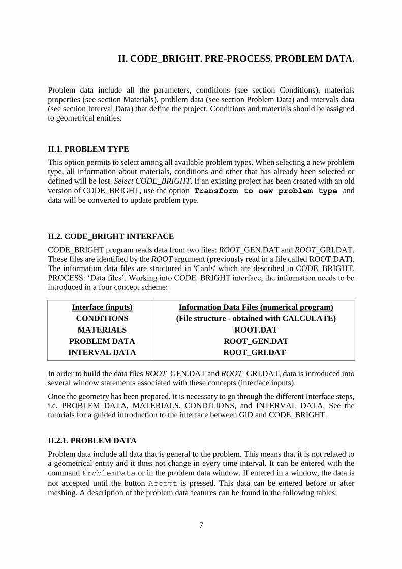
II.2. CODE_BRIGHT INTERFACE
CODE_BRIGHT program reads data from two files: ROOT_GEN.DAT and ROOT_GRI.DAT.
These files are identified by the ROOT argument (previously read in a file called ROOT.DAT).
The information data files are structured in 'Cards' which are described in CODE_BRIGHT.
PROCESS: ‘Data files’. Working into CODE_BRIGHT interface, the information needs to be
introduced in a four concept scheme:
Interface (inputs)
CONDITIONS
MATERIALS
PROBLEM DATA
INTERVAL DATA
Information Data Files (numerical program)
(File structure - obtained with CALCULATE)
ROOT.DAT
ROOT_GEN.DAT
ROOT_GRI.DAT
In order to build the data files ROOT_GEN.DAT and ROOT_GRI.DAT, data is introduced into
several window statements associated with these concepts (interface inputs).
Once the geometry has been prepared, it is necessary to go through the different Interface steps,
i.e. PROBLEM DATA, MATERIALS, CONDITIONS, and INTERVAL DATA. See the
tutorials for a guided introduction to the interface between GiD and CODE_BRIGHT.
II.2.1. PROBLEM DATA
Problem data include all data that is general to the problem. This means that it is not related to
a geometrical entity and it does not change in every time interval. It can be entered with the
command ProblemData or in the problem data window. If entered in a window, the data is
not accepted until the button Accept is pressed. This data can be entered before or after
meshing. A description of the problem data features can be found in the following tables:

8
GENERAL DATA
Title of the problem Interface Default: Coupled problem in geological media
Execution Only data file generation: ROOT_gen.dat and ROOT_gri.dat are
built
Full execution: Calculation with the finite element program
CODE_BRIGHT is performed (default option)
Backup
(IMBACKUP in
root_gen.dat)
No Backup
Save Last: Allows restart the calculation from the last time step computed.
Information is saved in file root_save.dat
Save All: Allows restart the calculation from any time step computed.
Information is saved in different files root_tnum_save.dat for each interval
data computed (tnum). To restart the calculation, rename the file
root_tnum_save.dat to root_save.dat
Axisymetry
(IAXISYM in
root_gen.dat)
No, Around y-axis
In 2-D axisymetry the principal stresses are: r (radial), y (axial),
(circumferential)
Gravity X (2-D and 3-D) component Interface Default: 0.0
Gravity Y (3-D) component Interface Default: 0.0
Gravity Y (2-D) or Z (3-D) component Interface Default: -9.81
EQUATIONS SOLVED
Stress equilibrium (unknown
displacement u) (IOPTDISPL
in root_gen.dat)
Yes, No
Updated lagrangian
method (IUPDC in
root_gen.dat)
Yes, No. Updated lagrangian method, i.e. coordinates are modified after
each time increment is solved. If deformations are very large, some
elements may distort. If distortion is very large the volume of an element
may become negative and the execution will terminate immediately.
Mass balance of water (unknown liquid
pressure Pl) (IOPTPL in root_gen.dat) Yes, No
Constant Pl Constant liquid phase pressure for problems not including the
mass balance of water equation
Mass balance of air (unknown liquid
pressure Pg) (IOPTPG in root_gen.dat) Yes, No
Constant Pg Constant gas phase pressure for problems that do not include
the equation of mass balance of air. Usually equal to 0.1 MPa.
Dissolved air into liquid phase
(IOPTXAL in root_gen.dat) Allowed, Not allowed
Energy balance (unknown temperature)
(IOPTTEMP in root_gen.dat) Yes, No
Vapour into gas phase (IOPTXWG in
root_gen.dat) Allowed, Not Allowed
Constant Temp Constant temperature for problems that do not include the
equation of energy balance.
Mass balance of conservative species
(unknown concentration) (IOPTXWS in
root_gen.dat)
Yes, No

9
Combinations of solving options are described below:
Pl Pg T Variable
1 0 0 Compressible water flow, one phase, one species, air is not considered.
0 1 0 Compressible air flow, one phase, one species.
0 0 1 Heat flow (only conduction).
1 1 0 Two phase flow (liquid + gas), air dissolved permitted, vapour not permitted.
1 0 1 Water two phase non-isothermal flow, vapour allowed, gas phase at constant
pressure.
0 1 1 Compressible non-isothermal gas flow, one phase, one species.
1 1 1 Non-isothermal two phase (liquid + gas) flow, vapour and air dissolved are allowed.
SOLUTION STRATEGY
Epsilon (intermediate time for
nonlinear functions)
Position of intermediate time tk+for matrix evaluation, i.e.
the point where the non-linear functions are computed.
(usual values: 0.5, 1). See details on Numerical Method.
Default: 1.0
Theta (intermediate time for
implicit solution) Position of intermediate time tk+for vector evaluation, i.e.
the point where the equation is accomplished. Default: 1.0
Time step control
(ITIME in root_gen.dat)
Default: 1
0-4: Time step control based on N-R iterations:
0: no time step prediction is performed.
1: predicts time stepping according to a limit of 4 iterations.
2: predicts time stepping according to a limit of 3 iterations.
3: predicts time stepping according to a limit of 2 iterations.
4: predicts time stepping according to a limit of 1 iteration.
6-9: Time step control based on error estimation:
6: controls time stepping by means of a prediction based on
the relative error deviation in the variables (relative error
lower than 0.01).
7: same as 6 but with a tolerance equal to 0.001.
8: same as 6 but with a tolerance equal to 0.0001.
9: same as 6 but with a tolerance equal to 0.00001.
Note: a time step control = 1 will always be considered for
negative time.
Max. number of iterations per
time step (ITERMAX in root_gen.dat)
Maximum number of Newton Raphson iterations per time
step. If the prescribed value is reached, time step is reduced.
Default: 10
Solver type
(ISOLVE in root_gen.dat)
Direct: LU + BACK
Iterative: Sparse + CGS
Solver type =
Iterative: Sparse +
CGS
Max number of solver iterations Default: 5000
Max abs solver error variable Default: 1.e-9
Max abs solver error residual Default: 0
Max rel solver error residual Default: 0

10
Elemental relative
permeability
computed from:
(IOPTPC in
root_gen.dat)
Elemental suction (consistent approach)
Average nodal degrees of saturation (default)
Average nodal relative permeabilities
Average nodal relative permeabilities (applies also for derivatives)
Maximal nodal relative permeability
Stress equilibrium
(unknown
displacement u) = yes
Max Abs Displacement (m)
(DELMXU in root_gen.dat)
Maximum (absolute) displacement error tolerance (m). When correction of displacements (displacement difference between two iterations) is lower than this value, convergence has been achieved. Default: 1e-6
Max Nod Bal Forces (MN)
(DELFMX in root_gen.dat)
Maximum nodal force balance error tolerance (MN). If the residual of forces in all nodes are lower than this value, convergence has been achieved. Default: 1e-10
Displacement Iter Corr (m)
(DUMX in root_gen.dat)
Maximum displacement correction per iteration (m) (time increment is reduced if necessary). Default: 1e-1
Mass balance of water
(unknown liquid
pressure Pl) = yes
Max Abs Pl (MPa)
(DELMXPL in root_gen.dat)
Maximum (absolute) liquid pressure error tolerance (MPa). Default: 1e-3
Max Nod Bal Forces (MN)
(DELQWMX in root_gen.dat)
Maximum nodal water mass balance error tolerance (kg/s). Default: 1e-10
Pl Iter Corr (MPa)
(DPLMX in root_gen.dat)
Maximum liquid pressure correction per iteration (MPa) (time increment is reduced if necessary). Default: 1e-1
Mass balance of air
(unknown liquid
pressure Pg) = yes
Max Abs Pg (MPa)
(DELMXPG in root_gen.dat)
Maximum (absolute) gas pressure error tolerance (MPa). Default: 1e-3
Max Nod Air Mass (kg/s)
(DELQAMX in root_gen.dat)
Maximum nodal air mass balance error tolerance (kg/s). Default: 1e-10
Pg Iter Corr (MPa)
(DPGMX in root_gen.dat)
Maximum gas pressure correction per iteration (MPa) (time increment is reduced if necessary). Default: 1e-1
Energy balance
(unknown
temperature) = yes
Max Abs Temp (C)
(DELMXT in root_gen.dat)
Maximum (absolute) temperature error tolerance (C). Default: 1e-3
Max Nod Energy (J/s)
(DELQMX in root_gen.dat)
Maximum nodal energy balance error tolerance (J/s). Default: 1e-10
Temp Iter Corr (C)
(DTMX in root_gen.dat)
Maximum temperature correction per iteration (C) (time increment is reduced if necessary). Default: 1e-1
Mass balance of
conservative species
(unknown
concentration) = yes
Max Abs Solute
(DELMXI in root_gen.dat)
Maximum (absolute) concentration error tolerance.Default: 1e-3
Max Nod Solute mass balance
(DELIMX in root_gen.dat)
Maximum nodal solute mass balance error tolerance.Default: 1e-10
Solute Iter Corr
(DIMX in root_gen.dat)
Maximum solute concentration correction per iteration (time increment is reduced if necessary). Default: 1e-1

11
Comments regarding the use of tolerances
In order to illustrate the use of tolerances the thermal problem is considered with the following
tolerances:
Max Abs Temp (C) T1
Max Nod Energy (J/s) T2
Temp Iter Corr (C) T3
Convergence can be achieved in two ways: the one when T < T1 for all nodes (condition A)
and the second when (qh < T2) also for all nodes (qh represents here the energy balance or
residual at a node) (condition B).
It is to be mentioned that convergence in terms of T and convergence in terms of qh should be
reached simultaneously because the Newton - Raphson method is used. For this reason, the
program stops the iteration process when one of the two conditions (A or B) is achieved.
When more than one degrees of freedom are solved per node and one of the recomended options
is used (convergence by variable OR residual), convergence in terms of variable or residual
should be achieved by all the variables simultaneously. In other words, it is not possible that
the mechanical problem converges by residual and the thermal problem converges by the
variable.
Finally, if (T > T3), time increment will be reduced. This parameter controls the accuracy of
the solution in terms of how large time increments can be. A low value of T3 will force to use
small time increments when large variations of temperature take place.
OUTPUT
Write
numerical
process
information
(IOWIT in
root_gen.dat)
Iteration information is written in file ROOT_GEN.OUT according to:
NONE: no information about convergence is written. This option should
be used if the user is very confident with the time discretization and not
interested in details at every time step or problems with time increment
reductions. Usually this happens when previous runs have shown that
convergence and time discretization work very well.
PARTIAL: partial information is written. Time intervals and time-values,
number of iterations, CPU-time values, etc. are written. Convergence
information (e.g. residuals) is only written if time increment reductions
take place.
ALL: all iteration information is written. Convergence information is
written for all iterations and all time increments. This option may result
in a very large file ROOT_GEN.OUT

12
Writing
frequency
(INTER in
root_gen.dat)
Writing results frequency in output files according to the number of time steps
(positive integer value) or according to a given time increment (negative integer
value).
If it is positive, e.g. is set to 20, results for the complete mesh will be written
only every 20 calculated time increments.
If it is negative, then we can obtain the output values in a specified time: e.g.
setting a value of -10 will produce output for 0, 10, 20, 30, … units of time.
Note that you may need to set a suitable maximum time step in the interval data
in order for this implementation to work well (the maximum time step should
be around one order of magnitude lower than the writing time frequency). See
Figures II.2.1a, b and c.
Figure II.2.1a. Writing every 20 time steps (Writing frequency = 20).
Figure II.2.1b. Writing every 20 time steps (Writing frequency = 100).
Writing every
20 time steps
Writing every
100 time steps

13
Figure II.2.1c. Writing every 10 days (Writing frequency = -10 and days selected
in the interval data).
OUTPUT
(continuation)
Write piezometric head Yes, No
Write boundary flow
rates in additional file
No (Defaul option)
Use writing frequency
Write all
Write boundary
reactions in additional
file
No (Defaul option)
Use writing frequency
Write all
Output points
(IOWCONTOURS in
root_gen.dat)
Nodes
Gauss points: (Default option)
Write all information
(IWRALL in
root_gen.dat)
Yes (default option), No
If No is selected, the following option appears:
Separated output files (IPOLYFILES in root_gen.dat) : Yes, No
and user go to Select output window.
Writing every 10 days (input -10 as writting frequency
when using days as time units)

14
SELECT OUTPUT
(If Write all information=No)
Select outputs option is necessary when working with complex problems in which separated output
files are used to facilitate the post-processing. The following options are available:
Write Displacements
Write Liquid Pressure
Write Gas Pressure
Write Temperature
Write solute concentration
Write Halite Concentration
Write Vapour Concentration
Write Gas Density
Write Dissolved air concentration
Write Liq Density
Write porosity
Write Liquid Saturation Degree
Write heat fluxes: qT
Write liquid fluxes: qL
Write gas fluxes: qG
Write diffusive heat fluxes: iT
Write diffusive water fluxes: iL
Write diffusive air fluxes: iG
Write diffusive solute fluxes: isolute
Write Stresses
Write Effective sStresses
Write stress invariants
Write strains
Write strains invariants
Write P0s TEP model
History variables of Viscoplastic model
History variables of Joint model
History variables of Argillite model
History variables of BExM model
History variables of CASM model
Yes, No
Yes, No
Yes, No
Yes, No
Yes, No
Yes, No
Yes, No
Yes, No
Yes, No
Yes, No
Yes, No
Yes, No
Yes, No
Yes, No
Yes, No
Yes, No
Yes, No
Yes, No
Yes, No
Yes, No
Yes, No
Yes, No
Yes, No
Yes, No
Yes, No
Yes, No
Yes, No
Yes, No
Yes, No
Yes, No

15
II.2.2. MATERIALS
All materials must be defined from a generic material. The following steps show how to
assign materials and do modifications:
- Creating new materials: In order to create new materials, one should write a material
name and complet the necessary constitutive laws and do an Accept Data to validate the
data entered. It is necessary to create a material before assigning it on the geometry.
- Assignment must respect hierarchical structure of entities (i.e. cannot assign a material
on a line belonging to a surface that have just been identified with another material). This
type of error may create conflicts.
- Posterior modifications on the parameters of assigned materials do not require a re-
meshing process.
- Material names: When introducing a name for a material, it is strongly recommended to
avoid spaces or underscores (e.g. use mat1 instead mat_1 or mat 1). The use of spaces or
underscores ( _ ) might create conflicts when the material is read.
Constitutive Laws in CODE_BRIGHT
Properties for materials can vary at each interval or mantain constant. Every constitutive law is
defined with 3data types:
Number of intervals. A box near the constitutive law name should be used for this
purpose. Usually parameters will be entered only for the first interval.
Each constitutive law is differentiated by the index ICL. For instance, ICL=6 is the
retention curve. Groups of ICL are considered, for instance ICL=21 to 27 is used for the
thermoelastoplastic model for unsaturated soils.
Parameters for constitutive law. A series of parameters should be entered for each
constitutive law, these are: ITYCL, P1, P2, P3, P4, P5, P6, P7, P8, P9, P10. The first
one (ITYCL) is an integer that indicates which option among the available ones is used.
For instance, thermal conductivity, permits different options depending the type of
dependence of porosity and degree of saturation that is desired. P1 to P10 are numbers
that correspond to parameters in a given equation.
ITYCL P1 P2 P3 P4 P5 P6 P7 P8 P9 P10
A number indicates the intervals where the law will be defined. This number fixes the
number of lines for VALUES to be entered. Every Interval line assumes parameters of
INTERVAL DATA according to the same order.

16
The following constitutive laws are available:
HYDRAULIC AND
THERMAL CONSTITUTIVE
MODELS (a)
RETENTION CURVE
INTRINSIC PERMEABILITY
LIQUID PHASE RELATIVE
PERMEABILITY
GAS PHASE RELATIVE
PERMEABILITY
DIFFUSIVE FLUXES OF MASS
DISPERSIVE FLUXES OF
MASS AND ENERGY
CONDUCTIVE FLUX OF HEAT
MECHANICAL CONSTITUTIVE MODELS
ELASTICITY (b)
NONLINEAR ELASTICITY (b)
VISCOPLASTICITY FOR SALINE MATERIALS
(b)
VISCOPLASTICITY FOR SATURATED SOILS
AND ROCKS (b)
VISCOPLASTICITY - GENERAL (b)
DAMAGE-ELASTOPLASTIC MODEL FOR
ARGILLACEOUS ROCKS (c)
THERMOELASTOPLASTIC MODEL FOR SOILS
(d)
BARCELONA EXPANSIVE MODEL FOR SOILS
(e)
CASM’s FAMILY MODELS (f)
PHASE PROPERTIES (a)
SOLID PHASE PROPERTIES
LIQUID PHASE PROPERTIES
GAS PHASE PROPERTIES
EXCAVATION PROCESS (g)
Description of each law is included in Chapter VI.
Assign material
With this instruction, the material is assigned to the selected entities. If assigning from a
window, every time the assigned material changes, the button Assign must be pressed again.
The user must select the entity on which to assign the materials, i.e.: line, surface or
volume when working in geometry mode or directly over the elements when working in
mesh mode. It is recommended to assign the materials on the geometry entities rather than on
the elements.
If assigning from the command line, option UnAssignMat erases all the assignments of this
particular material.
When a mesh has been already generated, and changes in the assigned materials are required,
then it is necessary to re-mesh again or assign the materials directly on the mesh.
Draw material
Draws a color indicating the selected material for all the entities that have the required material
assigned. It is possible to draw just one or draw all materials. To select some of them the users
should use a:b and all material numbers that lie between a and b will be drawn.
When drawing materials in 3 dimensions, it may be necessary to change the viewing mode to
polygons or render (see section Render) to diferenciate the front and back of the objects.
Unassign material
Command Unassign unassigns all the materials from all the entities. For only one material,
use UnAssignMat (see section Assign material).

17
New material
When the command NewMaterial is used, a new material is created taking an existing
one as a base material. Base material means that the new one will have the same fields as the
base one. Then, all the new values for the fields can be entered in the command line. It is
possible to redefine an existing material.
To create a new material or redefine an existing one in the materials window, write a new name
or the same one and change some of the properties. Then push the command Accept.
Element types in CODE_BRIGHT
When an element is selected to generate a finite element mesh it has to be available in
CODE_BRIGHT. The types of elements available in CODE_BRIGHT are:
DIM=2
TYPE 1
Linear triangle: mainly used in flow problems, i.e. when the
mechanical problem is not solved. Linear triangles are not
adequate for incompressible media. Analytical integration.
TYPE 12 Quadratic triangle. Corner nodes: 1, 2, 3; side nodes: 4, 5, 6.
Numerical integration with 3 internal points.
TYPE 5
Linear quadrilateral. Selective integration by means the
modification of the matrix B (Hughes, 1980). This avoids
locking when the medium is highly uncompressible. Numerical
integration with 4 points (recommended quadrilateral element).
TYPE 16 Zero thickness or joint element.
TYPE 8 Segment with a default thickness of 0.001 m and a default
porosity of 0.9.
DIM=3
TYPE 1
Linear tetrahedron. Analytical integration.
For n1 ≠ n2 ≠ n3 = n4 a triangular element is recovered.
A default thickness of 0.001 m is considered.
TYPE 26 Linear triangular prism. Numerical integration with 6 points.
TYPE 3 Linear quadrilateral prism element. Numerical integration
(selective) with 8 points.
TYPE 33
Quadratic tetrahedron. Numerical integration with 4 integration
points.
These types of elements are assigned by the interface between GiD and CODE_BRIGHT.
Note that linear triangular elements or linear tetrahedrons, which have been proven to be very
adequate for flow problems, should be avoided for mechanical problems. This is because if the
medium is nearly-incompressible (creep of rocks takes place with very small volumetric
deformation), locking takes place (not all displacements are permitted due to element
restrictions).

18
II.2.3. CONDITIONS
Conditions are all the properties of a problem –excluding materials– that can be assigned to an
entity. In this concept several types of conditions have been included: Force/displacement
conditions, flux conditions, initial unknowns, porosity (and other variables), initial stress, joint
element width, time evolution location, etc. The condition window permits to choose entities
to assign on (Point, Line, Surface or Volume in geometry display mode; and Node or Element
in mesh display mode) and select different types of conditions. It must be taken into account
that conditions assigned in mesh display mode will be unassigned in every new meshing
process.
In addition, the following points should be taken into account:
Force/displacement conditions add up all conditions assigned at every node, except for
variables Index (takes last value encountered) and Multiplier (takes the biggest).
Flux conditions, initial unknowns, porosity (and other variables), initial stress and joint
element width are assigned with entities priority from lower to higher level i.e. in the
following order: Points, Lines, Surfaces and Volumes (i.e. the node takes a
Flux_Point_B.C. refusing a Line_Flux_B.C. assigned previously).
When dealing with nodes shared by entities of the same level (e.g. surfaces) with different
initial values, it is recommended –especially in the case of thin interfaces– to assign
initial conditions on the entities containing those shared nodes (e.g. lines), so we are
able to effectively control the initial values on those nodes.
If a mesh has already been generated, for any change in the condition assignments, it is
necessary to re-mesh again to transfer these new conditions to the mesh.
Conditions description
II.2.3.1 Force/displacement conditions
The mechanical boundary conditions only exist if the mechanical problem is solved (Solve
displacement). For each time interval only the types that undergo changes should be read.
X direction force/stress Value in MN or MN/m2 = MPa
Y direction force/stress Value in MN or MN/m2 = MPa
Z direction force/stress Value in MN or MN/m2 = MPa
X displacement rate prescribed Value in m/s

19
Y displacement rate prescribed Value in m/s
Z displacement rate prescribed Value in m/s
X direction prescribed
When selected, displacement rate will be
prescribed in the X direction. Its value is
given in the cells above.
Y direction prescribed
When selected, displacement rate will be
prescribed in the Y direction. Its value is
given in the cells above.
Z direction prescribed
When selected, displacement rate will be
prescribed in the Z direction. Its value is
given in the cells above.
multiplier)
The units of this parameter depend on
whether force or stress is applied:
When applying a force: MN m
When applying a stress: MPa m
fxo obtained as ramp loading
during the current interval.
fyo obtained as ramp loading
during the current interval.
fzo obtained as ramp loading
during the current interval.
The general boundary condition is applied by means a forces/stresses computed as:
0
0
0
o
x x x x
o
y y y y
o
z z z z
f f u u t
f f u u t
f f u u t
This condition incorporates a von Newman type boundary condition plus a Cauchy type
boundary condition. A very large value of can be used to impose a fixed displacement rate. If
displacement rate is zero ( 0 0u ) and is very large, displacement is not permited in that
direction.
If is insufficiently large, however, the prescription of the displacement rate will be inaccurate.
On the contrary, extremely large values can cause matrix ill conditioning. Each specific
problem requires an adjusted value if displacement rate should be prescribed.
Depending on the geometric entity on which the condition should be applied, the following
options are encountered:
Points (2-D or 3-D) Lines (usually 2-D) Surfaces (usually 3-D) Volumes (3-D)
Forces Forces
Boundary stresses
Forces
Boundary stresses
Forces

20
II.2.3.2 Flux Boundary Condition
Mass or heat transport problems. These conditions only exist if any balance (water, air, energy
flow) problem is solved. For each time interval, only the types that undergo changes need to be
read.
The boundary condition is incorporated by adding a flux or flow rate. The mass flux or flow
rate of species i = w as a component of phase = g (i.e. the inflow or outflow of vapour) is
calculated as:
j j P Pg
w
g
w
g g
w
g g g g g g
w
g g
w
00
00
0
where the superscript 0 stands for the prescribed values, is mass fraction, is density, Pg is
gas pressure, jg0 is a prescribed gas flow and g and g are two parameters of the boundary
condition. Particular cases of this boundary condition are obtained for instance in the following
way:
Description (gw)0 jg
0 g Pg0 (g) g
A prescribed mass flow rate of gas with 0.02 kg/kg of
vapor and 0.98 kg/kg of air is injected
0.02 1e-5
kg/s
If Pg < Pg0 = 0.1 => a variable mass flow rate of gas
with 0.02 kg/kg of vapor and 0.98 kg/kg of air is
injected.
If Pg < Pg0 = 0.1 => a variable mass flow rate of gas
with variable composition outflows.
0.02 10 0.1
Humidity in the boundary is prescribed to 0.0112
kg/m3. This is equivalent to a relative humidity of
0.0112/0.0255 = 0.44 = 44%
0.01 1.12 10
Vapour pressure at T = 27 oC is calculated as:
136075exp( 5239.7 /(273 )) 0.003536 MPa = 3536 Pavp T
and the corresponding density is:
33536Pa 0.018 kg/mol0.02551 kg/m
(273 ) 8.3143 J/mol/K (273 27)K
vv
p M
R T
Associated to the same parameters but for component air, the following equation can be written:
0 0 0
0 0a a a a a
g g g g g g g g g g g gj j P P
where:
0 0
1a w
g g
which comes from the mass fraction definition.
On the other hand, for liquid phase a similar set of equations can be considered. These are:
0 0 0
0 0a a a a a
l l l l l l l l l l l lj j P P
0 0 0
0 0w w w w w
l l l l l l l l l l l lj j P P
0 0
1w a
l l

21
Positive values of mass flow rate indicate injection into the medium.
For energy, the boundary condition has the general form:
...)(00 w
g
w
geee jETTjj
In other words, a von Newman type term plus a Cauchy type term and a series of terms that
represent the energy transfer caused by mass inflow and outflow through the boundary.
The set of parameters that are required for these equations are (note that the symbols used by
Gerard et al., 2009, are not the same):
gw Prescribed mass fraction (kg/kg)
jg Prescribed gas flow rate*
jg Prescribed increment of jg during the time step*
Pg Prescribed gas pressure (MPa)
Pg Prescribed increment of Pg during the time step (MPa)
g Parameter for gas pressure term*
g Parameter for humidity term*
g Prescribed gas density (kg/m3)
l h Prescribed solute concentration (kg/kg)
l a Prescribed mass fraction of air (kg/kg)
jl Prescribed liquid flow rate*
jl Prescribed increment of jl during the time step*
Pl Prescribed liquid pressure (MPa)
Pl Prescribed increment of Pl during the time step (MPa)
l Parameter needed to be 0 when Pl is prescribed*
l Parameter needed only when mass transport problem is considered*
l Prescribed liquid density (kg/m3)
je Prescribed heat flow rate*
je Prescribed increment of je*
T Prescribed temperature (C)
T Prescribed increment of T during the time step (C)
e Parameter needed to be 0 when T is prescribed*
e Positive values: [ je = je exp (-abs (e) t) ] is used (1/s).
Negative values: [ je = je t-abs(e) ] is used (1/s).
Parameter for smoothing the seepage condition (outflow of water
only) boundary condition. * Units depend on problem dimension and parameter index. See Table II.2.1 (below) with a
summary of the units for each case.

22
For a positive value of a parabolic curve is used; for a negative value an exponentially
decaying curve is used. is the distance from the reference pressure to the point of change.
Index
(auxiliary
index)
+1.0 means that all flow rates are nodal values. For instance,
a pumping well boundary condition.
-1.0 means that all flow rates are per unit volume (3-D), area
(2-D) or length (1-D) of medium (internal source or
sink). For instance, a recharge due to rain in a 2-D case.
+2.0 means that all flow rates are per unit area (3-D) or
length (2-D) (lateral fluxes). For instance, lateral fluxes
from neighbour aquifers.
Prescribed gas, liquid and heat flows must be given in terms of flow units depending on the
way these flows are considered, i.e., depending on the kind of element they pass through and
on the problem dimension. The required units for each case are graphically specified below:
INDEX
PARAMETER
PROBLEM
DIMENSION ILLUSTRATION FLOW UNITS
Index = 1.0 3-D
Mass: kg
s
Heat: J
s
2-D
Mass:
kg
s
Heat: J
s
1-D
Mass: kg
s
Heat: J
s
Index = -1.0 3-D
Mass: kg
m3 s
Heat: J
m3 s
2-D Mass:
kg
m2 s
Heat: J
m2 s
1-D
Mass: kg
m s
Heat: J
m s

23
Index = 2.0 3-D
Mass: kg
m2 s
Heat: J
m2 s
2-D Mass:
kg
m s
Heat: J
m s
Table II.2.1. Summary of units used for different variables,
depending on problem dimension and parameter index
index Problem
dimension
Required units
Gas
flow
rate jg
Liquid
flow
rate jl
Parameters
g and l
Parameters
g and l
Heat
flow
rate je
Parameter
e
1.0 --- kg
s
kg
s
kg
s MPa
m3
s
J
s
J
s C
-1.0
1D kg
m s
kg
m s
kg
m s MPa
m3
m s =
m2
s
J
ms
J
m s C
2D kg
m2 s
kg
m2 s
kg
m2 s MPa
m3
m2 s =
m
s
J
m2 s
J
m2 s C
3D kg
m3 s
kg
m3 s
kg
m3 s MPa
m3
m3 s =
1
s
J
m3 s
J
m3 s C
2.0
2D kg
m s
kg
m s
kg
m s MPa
m3
m s =
m2
s
J
m s
J
m s C
3D kg
m2 s
kg
m2 s
kg
m2 s MPa
m3
m2 s =
m
s
J
m2 s
J
m2 s C
The fact that units are different for 3D, 2D and 1D is due to the reduction of one dimension in
2D and two dimensions in 1D. However, if a 2D model is considered to have 1 m associated
thickness, then units would be identical as in 3D. Similarly, if a 1D model is considered to have
1 m2 associated surface then units would be identical as in 3D.
The above boundary conditions are rather general. They incorporate terms of von Newman type
and Cauchy type. The equation includes three terms. The first one is the mass inflow or outflow
that takes place when a flow rate is prescribed at a node. The second term is the mass inflow or
outflow that takes place when a phase pressure is prescribed at a node. The coefficient is a
leakage coefficient. This variable allows prescribing a pressure with more or less strength. If
is very large, pressure will tend to reach the prescribed value (see Figures II.2.2 and II.2.3).
However, an extremely large value can produce matrix ill conditioning and a lower one can
produce inaccuracy in prescribing the pressure. However, it is not difficult to guess adequate

24
values for a given problem simply by trial. The third term is the mass inflow or outflow that
takes place when species mass fraction is prescribed at a node.
A surface where seepage (only outflow for liquid phase is permitted) is a case that may be of
interest. To indicate that only outflow is permitted l is entered with negative sign. This negative
sign only indicates that nodes with this kind of boundary condition allow seepage (i.e. only
outflow).
If there is inflow of gas or liquid phase, it is very important to give values of the following
variables: (gw)
o, (l
a)o, (l)
o, (g)
o and T
o. Otherwise, they are assumed to be zero, which is
not correct because they will be too far from equilibrium. If outflow takes place, this is not
relevant because the values of the medium are used instead of the prescribed ones.
qi
Pi
Poi
i
1.0
outflow
inflow
i > 0
Figure II.2.2
Figure II.2.3
qi
Pi
Poi
outflow
inflow
i < 0
i
1.0
25
Boundary conditions variable with time.
a) One boundary condition variable with time.
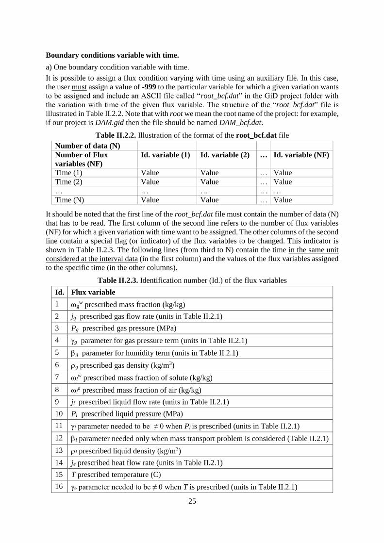
It is possible to assign a flux condition varying with time using an auxiliary file. In this case,
the user must assign a value of -999 to the particular variable for which a given variation wants
to be assigned and include an ASCII file called “root_bcf.dat” in the GiD project folder with
the variation with time of the given flux variable. The structure of the “root_bcf.dat” file is
illustrated in Table II.2.2. Note that with root we mean the root name of the project: for example,
if our project is DAM.gid then the file should be named DAM_bcf.dat.
Table II.2.2. Illustration of the format of the root_bcf.dat file
Number of data (N)
Number of Flux
variables (NF)
Id. variable (1) Id. variable (2) … Id. variable (NF)
Time (1) Value Value … Value
Time (2) Value Value … Value
… … … … …
Time (N) Value Value … Value
It should be noted that the first line of the root_bcf.dat file must contain the number of data (N)
that has to be read. The first column of the second line refers to the number of flux variables
(NF) for which a given variation with time want to be assigned. The other columns of the second
line contain a special flag (or indicator) of the flux variables to be changed. This indicator is
shown in Table II.2.3. The following lines (from third to N) contain the time in the same unit
considered at the interval data (in the first column) and the values of the flux variables assigned
to the specific time (in the other columns).
Table II.2.3. Identification number (Id.) of the flux variables
Id. Flux variable
1 gw prescribed mass fraction (kg/kg)
2 jg prescribed gas flow rate (units in Table II.2.1)
3 Pg prescribed gas pressure (MPa)
4 g parameter for gas pressure term (units in Table II.2.1)
5 g parameter for humidity term (units in Table II.2.1)
6 g prescribed gas density (kg/m3)
7 lw prescribed mass fraction of solute (kg/kg)
8 la prescribed mass fraction of air (kg/kg)
9 jl prescribed liquid flow rate (units in Table II.2.1)
10 Pl prescribed liquid pressure (MPa)
11 l parameter needed to be ≠ 0 when Pl is prescribed (units in Table II.2.1)
12 l parameter needed only when mass transport problem is considered (Table II.2.1)
13 l prescribed liquid density (kg/m3)
14 je prescribed heat flow rate (units in Table II.2.1)
15 T prescribed temperature (C)
16 e parameter needed to be ≠ 0 when T is prescribed (units in Table II.2.1)

26
b) Multiple boundary conditions variable with time.
For a value in a flux boundary condition that varies with time according to a function of time
(list of values) the following actions have to be taken:
Set de value of the variable equal to -99901.
If you have more values for the same boundary condition or in another boundary condition,
use the values -99902, -99903 up to -99999 if necessary.
Prepare a file (root_bcf.dat) with the following structure:
- First row: m, number of data values to be read (lines).
- Second row: –n 1 2 3 … n where n ≤ 99 number of variables that change with time.
- m rows with time_1 value_1 time_2 value_2 … time_n value_n.
II.2.3.3 Atmospheric boundary conditions module in CODE_BRIGHT
Introduction
Within Flux Boundary conditions in CODE_BRIGHT, the particular case of atmospheric
boundary conditions1 is eligible. These conditions encompass mass and heat conditions (in
terms of atmospheric data) and supposes that mass and heat transport problems are to be solved.
Atmospheric conditions are accessible from the “Flow rate” combo box in GID or setting
index=5 (and giving the parameters as described in Table II.2.4) in CardGroup 20.
Atmospheric boundary condition option allows to impose boundary conditions in terms of
evaporation, rainfall, radiation and heat exchanges thus simulating the complex soil-atmosphere
interactions. These phenomena are expressed as flux boundary conditions for the three
components (water, air and energy) as functions of the state variables (liquid pressure, gas
pressure and temperature of the soil) or dependent variables (liquid saturation degree, fraction
of water in the gas phase) and meteorological data that vary in time (atmospheric temperature
and pressure, relative humidity, solar radiation, cloud index, rainfall and wind velocity).
Conventions used in this paper are:
a file name is typed in an italic shaped font,
a subroutine name or a variable is typed using Courier font,
a files names in parentheses after a subroutine name refers to the file in which the
subroutine is implemented.
Overview of the module
The file bcond_atmos.f contains 3 subroutines:
atmosferic_boundary_condition
get_atm_data
sun
Figure 4 presents a general algorithm of atmosferic_boundary_condition
subroutine.
1The first implementation of this module is due to Maarten Saaltink.

27
The calls to atmosferic_boundary_condition subroutine appear in the following
subroutines:
atm_boundary_conditions (bcond_flow.f) itself called by newton_raphson
(nr.f)
write_boundary_flows (write.f) itself called by main_calculate
(code_bright_main.f)
Running atmosferic_boundary_condition needs index=52 as boundary condition
type, this latter being passed in FLUX(20). FLUX vector is read from file root_gen.dat by
read_boundary_conditions (read_general.f). The index of this file is iin1 (the
concerned card is numbered 20).
It should be noted that flow rates computed by the atmosferic_boundary_condition
subroutine are then treated as if index = 2.0 (used in classic flux boundary conditions)
were set i.e. as if flow rates are per unit area.
Figure II.2.4: General algorithm of atmosferic_boundary_condition.
(*) Subroutine sun is called if and only if ISUN1.
2This variable is locally called ICON.
call get_atm_data
flux of gas
flux of water
evaporation
vapour via gas
vapour via liquid flux of air
energy flux
per radiation
per advection
per convection
call sun write to output
BEGIN
END
(*)

28
Input data
Problem data definition file (root_gen.dat)
When atmospheric boundary conditions are considered, the parameters presented in Table II.2.4
have to be entered in CardGroup 20 in file root_gen.dat. These conditions are activated via
FL20, which should be set to 5. In Table II.2.4, latitude, time when autumn begins, time at
noon, dry and wet albedos are used for calculating radiation when radiation type is lower than
3.
Roughness length, screen height and stability factor are used for evaporation estimation and for
estimation of the advective energy flux.
Table II.2.4: Parameters to be entered in CardGroup 20.
FL1 Latitude (rad), λ
FL2 Time when autumn starts (s), ts
FL3 Time at noon (s), tm
FL4 Roughness length (m), z0
FL5 Screen height (m), za
FL6 Stability factor (-),
FL7 Atmospheric gas density (kg.m-3), ga
FL8 Dry albedo (-), Ad
FL9 Wet albedo (-), Aw
FL10 Gas leakage coefficient (kg.m-2.s-1.MPa-1), γg
FL11 Liquid leakage coefficient (kg.m-2.s-1.MPa-1), γl
FL12 Factor with which rain is multiplied (-), krain
FL13 Factor with which radiation is multiplied (-), krad
FL14 Factor with which evaporation is multiplied (-), kevap
FL15 Dip (rad)
FL16 Strike (rad)
FL17 Unused
FL18 Unused
FL19 = 0.0: radiation is calculated (see section 0)
= 3.0: radiation data are read from input file root_atm.dat
FL20 index=5 means atmospheric boundary conditions
Table II.2.5 presents ranges of roughness lengths for different types of surfaces from which
evaporation has to be calculated.
Table II.2.5: Roughness lengths for different types of surfaces after Chow et al. (1988).
Type of surface Height main roughness (m)
Ice, mud flats 1.10-5
Water 1.10-4 – 6.10-4
Grass (up to 10 cm high) 1.10-3 – 2.10-2
Grass (10 to 50 cm high) 2.10-2 – 5.10-2
Vegetation (1–2 m) 0.2
Tress (10 – 15 m) 0.4 – 0.7

29
Atmospheric data input file (root_atm.dat)
General parameters are to be entered in the problem data file (see CardGroup 20 description
here above) but time varying atmospheric data which are required to compute mass and heat
fluxes should be entered within an ASCII file called root_atm.dat3. Data that can be read is
summarized in Table II.2.6.
For each variable, the pair of columns containing available data is organised is the way
schematically presented in Table II.2.4. More details about this file and time varying
atmospheric data are given is section 0, dedicated to get_atm_data subroutine.
Figure II.2.5: Screenshot of GID atmospheric boundary conditions window.
3The file root_atm.dat is read with a free format. A dedicated tool developed by J.M. Pereira
(atmdata.exe) can be used to check its general format.
4In this table, light grey and bold grey cells respectively identify measured data and unused data
(the former being constituted of time (ti) and corresponding values (xi) pairs for each quantity).

30
Table II.2.6: Time varying atmospheric data to be provided in file root_atm.dat.
Data Unit
Atmospheric temperature, Ta °C
Atmospheric gas pressure, Pga MPa
Relative humidity, Hr -
Radiation5, Rm J m-2 s-1
Cloud index6, In -
Rainfall, P kg m-2 s-1
Wind velocity, va m s-1
Long wave Radiation7, Rl J m-2 s-1
Atmospheric transmissivity8, a -
Table II.2.7: Illustration of the format of root_atm.dat file (excluding first line).
Ta Pga Hr Rm In P va Rl a
Flag 0 0 0 0 0 0 0 0 0 0 0 0 0 0 0 0 0 0
Annual mean 0 x_am 0 x_am 0 x_am 0 x_am 0 x_am 0 x_am 0 x_am 0 x_am 0 x_am
Annual ampl 0 x_aa 0 x_aa 0 x_aa 0 x_aa 0 x_aa 0 x_aa 0 x_aa 0 x_aa 0 x_aa
Annual gap (s) 0 x_ag 0 x_ag 0 x_ag 0 x_ag 0 x_ag 0 x_ag 0 x_ag 0 x_ag 0 x_ag
Daily ampl 0 x_da 0 x_da 0 x_da 0 x_da 0 x_da 0 x_da 0 x_da 0 x_da 0 x_da
Daily gap (s) 0 x_dg 0 x_dg 0 x_dg 0 x_dg 0 x_dg 0 x_dg 0 x_dg 0 x_dg 0 x_dg
Unused 0 0 0 0 0 0 0 0 0 0 0 0 0 0 0 0 0 0
Measures… ti xi ti xi ti xi ti xi ti xi ti xi ti xi ti xi ti xi
Measures… ti xi ti xi ti xi ti xi ti xi ti xi ti xi ti xi ti xi
Measures… ti xi ti xi ti xi ti xi ti xi ti xi ti xi ti xi ti xi
Measures… ti xi ti xi ti xi ti xi ti xi ti xi ti xi ti xi ti xi
Measures… … … … … … … … … … … … … … … … … … …
5Radiation data will be used only if “Radiation type” is different from ‘0’ or ‘1’ in the boundary
conditions parameters. Rm will be the net radiation measurements if “Radiation type” is set
“3”, otherwise, if “Radiation type” is set to 2, 4 or 5 Rm will be the short wave (solar) radiation
measurements.
6Cloud index allows to account for a cloudy sky in the radiation computation (In = 1 for a clear
sky and In = 0 for a completely cloudy sky).
7Long wave (atmospheric) radiation data will be used only if “Radiation type” is set to 4 in the
boundary conditions parameters.
8Atmospheric transmissivity data will be used only if “Radiation type” is set to 0 or 1, or the
atmospheric boundary condition is apply to a inclined surface (dip > 0, FLUX(15)).
Atmospheric trasnmisivity expresses the amount of external radiation that is absorved by the
atmosphere, it can be estimated from the relative sunshine hours as 𝜏𝑎 = 0.25 + 0.50 𝑛 𝑁⁄ ,
where n is the hours of sunshine and N the hours of daylinght. Or, 𝜏𝑎 can be estimated from the
maximal (𝑇𝑎𝑚𝑎𝑥) and minimal (𝑇𝑎
𝑚𝑖𝑛) daily temperatrure as 𝜏𝑎 = 𝐾ℎ√𝑇𝑎𝑚𝑎𝑥 − 𝑇𝑎
𝑚𝑖𝑛 , where
Kh is an empirical constant, Kh = 0.16 for interior and Kh = 0.19 for coastal regions.

31
It should be noted that the first line of the file root_atm.dat must contain the number of lines
(excluding this one) and number of columns that has to be read. The second line refers to
interpolation or simulation option: it corresponds to a special flag allowing the user to simulate
the atmospheric data on the base of annual and daily characteristics that are furnished (see eq.
(23)). This simulation will be processed if, for a given quantity, its flag is set to ‘0’. The values
necessary to proceed to this simulation are provided in the 5 following lines and correspond to
annual mean, amplitude and gap and daily amplitude and gap. On the contrary, if this flag is set
to ‘1’, CODE_BRIGHT will use the measured data provided in the rest of the lines of the data
file and process to linear interpolations in order to obtain the value of a quantity for a given
calculation time.
Subroutines description
Subroutine atmosferic_boundary_condition
General description
This subroutine is the core of the atmospheric boundary condition module. It computes
atmospheric boundary conditions, including evaporation, rain, radiation, advective and
convective energy fluxes. Those are expressed in terms of fluxes of water, air and energy as
functions of the state variables (liquid pressure, gas pressure and temperature of the soil).
Moreover, the subroutine calculates the derivatives of these three fluxes with respect to the state
variables. Positive values always mean entering the system. Negative values always mean
leaving the system e.g. evaporation is negative.
It first calls get_atm_data to read atmospheric data which is stored in a matrix named
atmosferic9 (see subroutine get_atm_data for more information on the format of this
file). Some general parameters (like for instance dry and wet albedos) are read from FLUX, an
argument passed to the main subroutine (which corresponds to CardGroup 20 of the problem
data file root_gen.dat).
It then computes water flux (through gas and liquid phases, due to evaporation and rain), air
flux and energy flux (radiation, advective and convective energy fluxes). Optionally, it can
write these fluxes to files depending upon the presence of surveyed nodes or not. The general
equations for calculating these fluxes are now presented.
Fluxes of mass
- Flux of gas: The flux of the gas phase qg is given by the following equation, in which Pga is
the atmospheric pressure and g is a leakage coefficient:
gaggg PPq (1)
- Flux of air: For the flux of air ja only the advective part is considered:
g
w
gg
a
ga qqj 1 (2)
9Matrix atmosferic is stored in bb(n74).

32
- Flux of water: Evaporation E is given by an aerodynamic diffusion relation:
2
2
a
0
zln
z
ava v
k vE
(3)
where va and v respectively are the absolute humidity (mass of vapour per volume of gas,
which can be calculated from relative humidity Hr and temperature) of the atmosphere and at
the node of the boundary condition, k is the von Karman’s constant (often taken as 0.4), is a
stability factor, va the wind velocity, z0 is the roughness length, za is the screen height at which
va and va are measured. In theory, v must be the value at roughness length (z0). Instead, it is
calculated from the state variables at the node of the boundary condition. Hence, a constant
profile for v is assumed between this node and height z0.
The advective flux of vapour by the gas phase jgw is given by:
gagg
ga
vaw
g
gagg
w
g
w
g
PPqj
PPqj
if
if
(4)
where ρga is the atmospheric gas density and qg is the flux of the gas phase given by equation
(1).
Surface runoff jsr (which corresponds to the flow rate of water through the liquid phase jlw) is
written as:
galsr
galgalwsr
PPj
PPPPj
if0
if (5)
where γw is another leakage coefficient. It must be said that ponding is not explicitly simulated,
that is, CODE_BRIGHT does not have a special element representing storage of water in a
pond. When one assumes no ponding, a very high value for γw can be used (but not to high to
avoid numerical instabilities). Then, if the soil is saturated (Pl > Pga) all rainfall that cannot
infiltrate will runoff.
The flux of water jw is the sum of rainfall P, evaporation E and advective flux of vapour gas
phase jgw and of surface runoff jsr:
sr
w
gevaprainw jjEkPkj (6)
where coefficients krain and kevap are input data passed through FLUX and may be used to disable
their respective flux.

33
Flux of energy
- Radiation
Several options are available to evaluate radiation –using ISUN which is passed to the
subroutine by FLUX(19)–: 0 for horizontal plane, 1 for vertical cylinder, 2 for measured sun
radiation (only short wave radiation is considered), 3 for measured net radiation (short + long
wavelength radiations), 4 for measured atmospheric and solar radiation and 5 for measured sun
radiation (long and short wave radiations are considered). SUN subroutine is called only10 if
ISUN is lower or equal to 1.
The radiation Rn can be given as a measured data or it can be calculated, depending on the value
of ISUN:
{
𝑅𝑛 = (1 − 𝐴𝑙)𝑅𝑠 + 𝑅𝑎 − 휀𝜎𝑇
4 If ISUN ≤ 1 𝑅𝑛 = 𝑅𝑚 If ISUN = 2 or 3
𝑅𝑛 = (1 − 𝐴𝑙)𝑅𝑚 + 𝑅𝑙 − 휀𝜎𝑇4 If ISUN = 4
𝑅𝑛 = (1 − 𝐴𝑙)𝑅𝑚 + 𝑅𝑎 − 휀𝜎𝑇4 If ISUN = 5
(7)
where Rs is the direct solar short wave radiation, Ra is the long wave atmospheric radiation, Al
is the albedo, ε is the atmospheric emissivity, σ is the Stefan-Boltzman constant (5.67×10⁻⁸ J s-
1 m-2 K-4) Rm represents the values of measured radiation (net or solar according to the radiation
type) and Rl represents the values of measured atmosferic radiation (log wave). Rm and Rl are
read from file root_atm.dat by subroutine get_atm_data.
Both the albedo and emissivity are considered function of the liquid saturation Sl:
llwddl SSAAAA 22 (8)
lS05.09.0 (9)
where Ad and Aw are the dry and wet albedos.
The long wave atmospheric radiation Ra depends on the atmospheric temperature and absolute
humidity according to an empirical relation:
vaaa TR 1370048.0605.04 (10)
The calculation of the solar radiation Rs depends on the value of ISUN. Only the case of a
horizontal surface (ISUN=0) will be presented here. Rs for horizontal surface is simplified by:
{𝑅𝑠,ℎ𝑜𝑟 = 𝑆0𝑓𝑒𝜏𝑎(cos 𝛿 cos 𝜆 cos 𝜃 + sin 𝛿 sin 𝜆) 𝑖𝑓 𝑆𝑢𝑝 > 0
𝑅𝑠,ℎ𝑜𝑟 = 0 𝑜𝑡ℎ𝑒𝑟𝑤𝑖𝑠𝑒 (11)
Where, a is the atmospheric transmissivity, the latitude, S0 the sun costant (=1367 J m-2 S-1),
fe the correction factor related to the eccentricity of the earth’s orbit, the earth declination and
the solar angle.
fe can be calculated from (Allen et all., 1998) as:
𝑓𝑒 = 1 + 0.033 cos (𝑡−𝑡𝑝ℎ
𝑑𝑎) (12)
10 For other cases (ISUN = 2, 3, 4 or 5), RAD_DIR is set to values read from root_atm.dat by
subroutine get_atm_data.

34
where, da is the year duration (= 365.241 days = 3.15568×10⁷ s), tph is the time at perihelion
(January 3d)
The sun declination (δ) is the angle between the direction of the sun and the equator. It can be
calculated by a yearly sinusoidal function:
𝛿 = 𝛿𝑚𝑎𝑥 sin (2𝜋𝑡−𝑡𝑠
𝑑𝑎) (13)
where max is the maximum sun declination (= 0.4119 rad = 23.26°), ts is time at September
equinox (September 21st for the northern hemisphere).
The solar angle (θ) describes the circular movement of the sun during a day. It equals 0, when
the sun is at its zenith and can be estimated as:
𝜃 =𝑡−𝑡𝑚−𝑡𝑐
𝑑𝑑2𝜋 (14)
where, tm is the time at noon for an arbitrary day, dd is the day duration (= 86400 s) and tc is the
equation of time, used to correct the variations on the hour of zenith during the year, and defined
as:
𝑡𝑐 =𝛿𝑚𝑎𝑥𝑑𝑑
8𝜋sin (
𝑡−𝑡𝑠
𝑑𝑎4𝜋) −
𝑒𝑑𝑑
𝜋sin (
𝑡−𝑡𝑝ℎ
𝑑𝑎2𝜋) (15)
where, e is the eccentricity to the earth’s orbit (=0.0167)
Subequations 2 to 5 in Eq. (7) use data read from root_atm.dat file. ISUN=2 suppose that only
radiation considered is measured solar radiation (short wave), ISUN=3, assumes that measured
data corresponds to net radiation (short + long wave length i.e. solar + atmospheric – surface),
ISUN=4, considers that data available are solar radiation (Rm in root_atm.data file) and
atmospheric radiation (Rl in root_atm.data file), while ISUN=5 considers that only data
available are solar radiation (short wave length, Rm in root_atm.data file)
Solar radiation (short wave) is measured or calculate on a horizontal surface, when an inclined
surface is considered this value must be corrected. The atmosphere scatters the sunlight, so the
surface receives part of the sun radiation directly from the sun and another part in a diffusive
form. An inclined surface in the shade does not receive the direct part but only the diffusive
solar radiarion.
Therefore, for an inclined surface the real solar radiation perceived can be obtained by the next
expression:
𝑅𝑠 = 𝑅𝑠,ℎ𝑜𝑟 [(1 − 𝑓𝑑𝑖𝑓)max (𝑃𝑇𝑠,0)
𝑆𝑢𝑝+ 𝑓𝑑𝑖𝑓] (16)
where, Rs,hor is the solar radiation on a horizontal surface (measured or calculated), fdif the
fraction of diffusive solar radiation over the total solar radiation, defined as:
𝑓𝑑𝑖𝑓 = 1
1+exp (8.6𝜏𝑎−5) (17)
Vectors P and S, are unitary length vectors that define the position of Sun and Zenith. P is
orthogonal to the earth surface pointing outwars and S points to the Sun, they are defined as
follows:
𝑃 = (
𝑃𝑒𝑎𝑠𝑡𝑃𝑛𝑜𝑟𝑡ℎ𝑃𝑢𝑝
) = (−
cos𝛼 sin 𝛽sin 𝛼 sin 𝛽cos 𝛽
) (18)

35
𝑆 = (
𝑆𝑒𝑎𝑠𝑡𝑆𝑛𝑜𝑟𝑡ℎ𝑆𝑢𝑝
) = (cos 𝛿 sin 𝜃
sin 𝛿 cos 𝜆 − cos 𝜃 cos 𝛿 sin 𝜆cos 𝛿 cos 𝜆 cos 𝜃 + sin 𝛿 sin 𝜆
) (19)
where, and are the surface strike and dip, respectivelyThe product of both vectors (PTS)
equals the cosine of the angle between them. For horizontal surface ( =0) the vector
PT=(0,0,1) and PTS = Sup. At night Sup < 0, at daylight Sup > 0 and during the sunrise and
sunset Sup = 0.
- Advective energy flux
The sensible heat flux Hs is, like evaporation, calculated through an aerodynamic diffusion
relation:
2
2
0
a
zln
z
as ga a a
k vH C T T
(20)
where Ca is the specific heat of the gas.
- Convective energy flux
The convective or latent heat flux Hc is calculated taking into account the internal energy of
liquid water, vapour and air:
aa
l
wla
g
wvc jhjPhjEhH 0 (21)
where hv, hla and ha0 are the free energy of vapour, liquid water and air, respectively. These
three properties depend on the temperature: temperatures used are the temperature at the node
of the boundary for hv, and ha0 and the dew point temperature, which depends on the
atmospheric vapour pressure, for hla.
- Total energy flux
The total energy flux je thus writes as follows:
csnrade HHRkj (22)
where krad is an input parameter passed through FLUX and may be used to disable radiation
flux.
Results output
If values are surveyed at a given node, the following variables are written to files
200+nodout: t+t, P, E, jwg, jw
l, jw, ja, Rn, Hs, Hc, je.

36
Subroutine get_atm_data
This subroutine computes atmospheric data at time t+dt either by simulation or by interpolation
of input data. In both cases, returned values are summarized in Table II.2.8. This table also
mentions implemented names for these variables and columns concerned in the matrix
atmosferic, where all data needed for simulations or interpolations are stored.
Two options can be used to compute atmospheric data: interpolation and simulation.
Interpolation uses a simple linear interpolation of the specified parameters versus time.
Simulation uses the following sinusoidal expression:
d
d
d
a
a
amd
ttx
d
ttxxtx 2sin2sin)( (23)
where x is the value of the parameter, xm is its mean value, aa is its annual amplitude, ad its daily
amplitude, ta is the start of the annual variation, td is the start of the daily variation, da is the
duration of a year and dd is the duration of a day (= 86400 s).
Table II.2.8: Atmospheric data taken into account in the boundary conditions module.
Atmospheric variable Unit Implemented name Columns used
Atmospheric temperature, Ta °C TEMP_ATM 1 – 2
Atmospheric gas pressure, Pga MPa PG_ATM 3 – 4
Relative humidity, Hr – RELHUM 5 – 6
Solar radiation, Rn J/m²/s RAD_DIR 7 – 8
Insolation fractions, In – FRACINS 9 – 10
Rain, P kg/m²/s RAIN 11 – 12
Wind velocity, va m/s WIND 13 – 14
Matrix atmosferic is read from file root_atm.dat (or root_atm.inp) which index is iin3
=103. This file is opened by read_assign_files subroutine (read_grid.f) and read by
read_atm_bc (read_general.f) subroutine which assigns atmosferic its values and is
called by main_initialize (code_bright_main.f).
Note that atmosferic dimensions also are read from iin3 and that this instruction is present
in read_assign_dim_opt_2 (code_bright_main.f).
Data simulation
If a simulation is performed, a sinus shape function with annual and daily variations is used.
The daily variation is only taken into account if the time increment is lower than one day. Input
data (for each variable) needed for each variable is (Unit represents the unit given in Table
II.2.8):
annual mean (Unit), xm, annual amplitude (Unit), xa, annual gap (s), ta, daily amplitude (Unit), xd, daily gap (s), td.

37
For a given variable, the simulated value a time t+dt is obtained according to the following
relation11:
dd
ddd
aa
aaam
d
dt
d
tdttdx
d
dt
d
tdttdx
dtxdttx
sin5.02
sin
sin5.02
sin1
)(
(24)
Figure II.2.6 and Figure II.2.7 show the simulation of the annual variation of an atmospheric
variable (case of temperature).
Data interpolation
Interpolation concerns all available data for discrete times ti satisfying t < ti+1 and t + dt > ti
until condition t + dt < ti+1 is satisfied. If code time t is lower (resp. bigger) than lowest (resp.
highest) discrete time, the subroutine is stopped.
Figure II.2.6: Simulation of annual variation of an atmospheric variable (case of temperature).
11 This expression cancels out daily variations if the time increment dt is higher than dd,
duration of one day.
0 50 100 150 200 250 300 350 4000
5
10
15
20
25
30Annual variation with and without daily variations
time (days)
Tem
pera
ture
(°C
)
with
without
Annual gap
Annual amplitude
Annual mean

38
Figure II.2.7: Simulation of annual variation of an atmospheric variable (case of temperature;
close view).
Subroutine SUN
This routine calculates the direct solar radiation. Calculation type (ISUN) is passed through
FLUX vector in atmosferic_boundary_condition. The different values for ISUN
that imply a call to SUN subroutine are:
0 - horizontal plane,
1 - vertical cylinder.
However, ISUN=0 is the unique option proposed in the manual of Retraso.
This calculation takes into account sun distance and declination (function of date from 1st
January), solar day duration (function of latitude and declination). All this data together with
insolation fraction allow computing daily radiation (equations where presented in section 0).
If time increment is bigger than a day, direct radiation directly uses daily radiation. Otherwise,
time with respect to night is taken into account and the direct radiation is calculated.
Figure II.2.8 shows the simulated daily radiation versus time in both cases.
Case ISUN=1
2
0 sinsincoscos112
s
sA
drSR (25)
170 175 180 185 190 195 20018
19
20
21
22
23
24
25
26
27
28
29Annual variation with and without daily variations
time (days)
Tem
pera
ture
(°C
)
with
without

39
Figure II.2.8: Daily radiation as a function of time according to ISUN option.
Reference
Chow, V. T., Maidment, D. R., and Mays, L. W. (1988). Applied Hydrology, McGraw-Hill.
II.2.3.4 Initial Unknowns
Initial values of the unknowns can be assigned on surfaces/volumes on the geometry. A constant
or linear distribution is available.
Distribution: Constant / Linear
Ux displacement Value in m
Uy displacement Value in m
Uz displacement Value in m
Liquid pressure: Pl Value in MPa
Gas pressure: Pg Value in MPa
Temperature: T Value in ºC
Concentration Value in kg/kg
If distribution is linear, information about unknowns’ values at final point and the coordinates
of the initial and final points are required.
In case of nodes with multiple initial conditions assigned, the ones assigned into entities of
higher levels prevail. It is recommended to assign the materials on the geometry entities, but
it is also possible to assign them directly into mesh elements in case is needed.
0
5
10
15
20
25
30
0 50 100 150 200 250 300 350 400
Time (days)
Dail
y R
ad
iati
on
(M
J/m
²)
Daily Rad ISUN 0 Daily Rad ISUN 1

40
II.2.3.5 Initial porosity
A constant initial value of porosity can be assigned on surfaces/volumes on the geometry.
Porosity value should be less than 1.
II.2.3.6 Initial stress
Initial values of the stresses and history variables (depends on the type of mechanical
constitutive model) can be assigned on surfaces/volumes on the geometry. A constant or linear
distribution is available.
Distribution: Constant / Linear
X stress Value in MPa
Y stress Value in MPa
Z stress Value in MPa
XY stress Value in MPa
XZ stress Value in MPa
YZ stress Value in MPa
History variable 1 (depend on the constitutive model)
History variable 2 (depend on the constitutive model)
In chapter VI, the description of history variables required for elastoplastic and viscoplastic
models is included.
If distribution is linear, information about stresses and history variables values at final point
and the coordinates of the initial and final points are required.
II.2.3.7 Initial anisotropy.
Transverse isotropy can be assigned on surfaces/volumes in a hydraulic, thermal and/or
mechanical problem. The direction of orthotropic axis is indicated by the two angles shown in
Figure II.2.9. Transformation is done from physical plane (global axes) to anisotropy directions
(local axes). First rotation is around z axis and the second rotation is around the new y’ axis.For
further help on how to model anisitropic properties please visit CODE_BRIGHT-Tutorial XVII
in the Tutorial Manual.
Parameters of elastic transverse isotropy can be assigned trough the Damage-elastoplastic
model for argillaceous rocks (ICL=71 to 79; see chapter VIc), while parameters of hydraulic
transverse isotropy can be assigned trough the intrinsic permeability law (ICL=7; see chapter
VIa).
First rotation:
(around z)
> 0 if directed from x to y
is the orientation of the dip with
respect to y (usually the North)
Second rotation:
(around y’)
> 0 if directed from z’ to x’
is the inclination of dip with respect to
the horizontal plane

41
Figure II.2.9: Convention of reference axis for transverse isotropic material.
II.2.3.8 Time Evolution
CODE_BRIGHT offers the user the possibility of registering the evolution with time of
specified problem variables either at specific points and surfaces/volumes on the geometry, or
at specific nodes and elements on the mesh. In case that nodes and elements are specified by
the user, special care must be taken when remeshing, yet information regarding time evolution
will be lost.
The program does not admit more than 10 nodes and 10 elements (or, if the case, points and
surfaces/volumes) for time evolution registration, whatever could be read from the introduced
time evolution data. These data, on the other hand, have to be given to the program as referring
to the first time interval of the problem.
However, Post–process interface in GID has available the information of problem variables in
all points/lines/surfaces/volumes of the geometry and nodes/elements of the mesh. Post–process
offers the option to draw graphs of specified problem variables. Several graph types are
available: point evolution against time, result 1 vs. result 2 over points, and result along a
boundary line (see View results/graphs option of Post-process). It is possible to save or read a
graph (see Files menu of Post-process). These advanced options of Post-process avoid the need
to select specific points/surfaces/volumes in conditions for the time evolution, before to run the
problem.
y
x
z
Cross-anisotropy plane
α
α
x
x’
y’=y’’ y
β
x’
x’’
z=z’ z’’
β

42
Assigning priorities
Conditions assigned on the geometry are distributed over the mesh with priorities. In general
points have priority over lines, lines over surfaces and surfaces over volumes. At mesh level,
nodes have priority over elements.
Mechanical boundary conditions on high entities are superimposed when they are applied to a
lower entity. This means, for instance in a 2-D case, that a point that belongs to two lines will
have the combination of boundary conditions coming from these two lines.
Assign condition
A condition is assigned to the entities with the given field values. If assigning from the
command AssignCond, the option Change allows the definition of the field values. Do not
forget to change these values before assigning. Option DeleteAll erases all the assigned
entities of this particular condition. Conditions can be assigned both on the geometry and on
the mesh but it is convenient to assign them on the geometry and the conditions will then be
transferred to the mesh. If conditions are assigned on the mesh, any remeshing will cause the
conditions to be lost.
Conditions that are to be attached to the boundary of the elements, are assigned to the elements
and GiD searches the boundaries of the elements that are boundaries of the total mesh. Option
Unassign inside AssignCond, permits to unassign this condition. It is also possible to
unassign from only certain entities.
If a mesh has already been generated, for any change in the condition assignments, it is
necessary to re-mesh again.
Draw condition
Option Draw all draws all the conditions assigned to all the entities in the graphical window.
This means to draw a graphical symbol or condition number over every entity that has this
condition. If one particular condition is selected, it is possible to choose between Draw and one
of the fields. Draw is like Draw all but only for one particular condition. If one field is
chosen, the value of this field is written over all the entities that have this condition assigned.
When the condition has any field referred to the type of axes, the latters can be visualized by
means of Draw local axes.
Unassign condition
In window mode, command UnAssign lets the user to choose between unassigning this
condition from the entities that owe it or unassigning all the conditions or select some entities
to unassign. In command mode UnAssing, do it for all the conditions. For only one condition,
use command Delete All (see section Assign condition).
Entities
Create an information window with all entities assigned including values at every one.

43
II.2.4. INTERVALS DATA
Intervals are a way to change some conditions and, eventually, material properties.
Properties for materials can vary at each interval or remain constant. For a problem with several
intervals, a window with more than one field can be used for each constitutive law (see figure
below). Each row represents the properties for each interval. If the number of the current
interval is higher than the number of rows, then the material will keep the properties of the last
row.
ITYCL P1 P2 P3 P4 P5 P6 P7 P8 P9 P10
In which a different line for each interval will appear. Usually, only the first line should be
filled. The following lines may be left in blank if material properties are unchanged.
Boundary conditions may vary at each interval or remain constant. For conditions the correct
way to proceed is to define all the invariable conditions first (i.e. those that remain unchanged
during all intervals). Then, it is allowed to define as many intervals as desired with the command
NewInterval or update the conditions in different intervals using the command
ChangeInterval. It is possible to define as many conditions as necessary into particular
intervals. The conditions which have not been duplicated when creating new intervals, are only
considered for their interval.
Interval data parameters, decribe temporal limits and time steps for each interval. They can be
entered with the command IntervalData or in the intervals data window. If entered in a
window, the data is not accepted until button Accept is pressed. This data can be entered
before or after meshing.
Description
INTERVAL DATA
Units of time discretization
Time units for defined interval. Options: Seconds,
Minutes, Hours, Days, Weeks, Months, Years
Initial Time (interval starts)
(TIMEI in root_gen.dat)
Initial time for the defined interval.
Initial Time Step
(DTIME in root_gen.dat)
Initial time step for this time interval.
Final Time (interval ends)
(TIMEF in root_gen.dat)
Final time for the defined interval.
Intermediate Time
(TIME1 in root_gen.dat)
Time from which time increment is kept below
the maximum allowed (advanced option).
Maximum Time Step
(DTIMEC in root_gen.dat)
Maximum allowed time step constant value.
Reset displacements to zero Yes / No
This option puts displacement to zero at the first
time step of the next time interval.

44
Using the advanced options, there is also possible to change the values of ‘epsilon’ or ‘time
step control’ for a given interval (these two variables have been explained in chapter II.2.1).
These changes will be mantained during the following intervals, unless the user explicitly
change them.
In 'Writing results frequency', the intermittence for writing results is defined, i.e. only after a
given number of time steps the results will be written. This may cause inconveniences if the
user desires the results at precisely fixed times (for instance: 6 months, 1 year, 2 year, etc.).
Moreover, if something changes between two runs (e.g. boundary conditions) and any time
increment should be modified, the value of the times in which results are output will not be
identical between these two runs. In this case, it would be difficult to make a comparison of the
two analyses because the output results correspond to different times.
However, it is possible to decide the values of the times for output using a sequence of
consecutive intervals. In this way, the results will be output for all 'Final time' defined, and if
the user is only interested in these fixed times a very large value may be used for 'Writing results
frequency' to avoid output at other times. Alternatively, this could be solved using a negative
‘writing frequency’ (see section II.2.1).
_________________________________

45
III.CODE_BRIGHT. PROCESS
III.1. CALCULATE
This part deals with the stage of the process that solves the numerical problem. The system
would allow calling the Finite Element program without necessity of leaving from the work
environment. Pressing Calculate the user can see a Process window, and clicking on Start
the solver module runs.
The option Calculate from the beginning is useful in case that you need to calculate
the project from the beginning (without using the saved files created in a previous calculate
process). WARNING: Calculate from the beginning option will erase all the save
type files from the working directory.
III.2. DATA FILES
If the solver program is required to be run outside GiD enviroment, i.e. in another computer or
the user needs to check the data input for calculations; it is posible to see the data files. In the
work directory there are the followings files: Root.dat ROOT_GEN.DAT ROOT_GRI.DAT
from which the program CODE_BRIGHT reads all the necessary data.
The name of these two files is composed by the extension .DAT which indicates that these files
contain input data, a suffix (_GEN or _GRI) that follows the ROOT and which indicates a file
with general information and a file with grid information, and a ROOT which is a name assigned
by the user. The ROOT is previously read in a file called ROOT.DAT. For a run with another
problem only this ROOT.DAT file must be changed and the files of the new problem will be
used.
III.3. GENERAL INFORMATION FILE ‘ROOT_GEN.DAT’
Card 1. Problem
Variables: HEAD
Format: (A40): Fixed format
-999: Free format
Card 2. Dimensions and options
Variables: NUMNP, NUMEL, NDIM, IAXISYM, NUMMAT, NHV
Format: (10I5). It is not required if free format is used
NUMNP: Number of nodes
NUMEL: Number of elements
NDIM: Space dimensions (1,2,3)
IAXISYM: Axisymmetric option: 0-no axisymmetry, 1-yes (around y-axis),
NDIM=2. The principal stresses are: r (radial), y (axial), (circunferential) NDIM=1. The principal stresses are: r (radial), (circumferential), z (axial)
NUMMAT: Number of materials
NHV: Number of history variables (depends on the type of mechanical constitutive
model used). This variable is checked internally.

46
Card 3. Dimensions and options
Variables: NZ1, NZ2, MFRONTH, NDF, MNVAL, ISOLVE
Format: (10I5). It is not required if free format is used
NZ1: = MXDIFN: maximum difference between connected nodes, this variable
is read for dimensioning purposes. The node numeration of the grid is
assumed to have been optimised in order to reduce the matrix band width.
If = = 0 are used in a non-mechanical problem, then MXDIFN can be
0 because a quasi-explicit approximation will be used, i.e. only a NDF-
diagonal matrix is solved which contains derivatives of the storage terms.
(See below for NZ = NZ1 * NZ2).
NZ2: = MBANDT: total band width (geometrical for 1 variable), (MBANDT =
2 (MXDIFN+1) - 1, the user should provide a value but the code checks
this value. So this entry is redundant.
NZ=
NZ1*NZ2:
Used only for ISOLVE = 5. It is the number of nonzero-blocks in the
jacobian (i.e. the number of nonzeros for NDF = 1). This variable is
computed as NZ = NZ1*NZ2. Since this variable is checked internally, if
the number of nonzeros is not known a priori, a guess can be used and the
code automatically checks its validity. Otherwise, the required value is
output.
MFRONTH: void
NDF: Number of degrees of freedom per node. For instance a 2-dimension
thermomechanical analysis requires NDF = 3.
MNVAL: Maximum number of integration points in an element (default = 1). For a
two-dimensional analysis with some (not necessarily all) quadrilateral
elements, MNVAL = 4. For a three-dimensional analysis with some (not
necessarily all) quadrilateral prism elements, MNVAL = 8.
ISOLVE: Solve the system of equations according to different algorithms.
ISOLVE = 3: LU decomposition + backsubstitution (NAG
subroutines, fonts available). Recommended option for direct solution.
ISOLVE = 5: Sparse storage + CGS (conjugate gradients squared).
Card 4. Dimension boundary conditions
Variables: NFDTYPE, NFLUXTYPE
Format: (5I5). It is not required if free format is used
NFDTYPE: Number of prescribed force/displacement boundary condition types.
NFDTYPE <= NUMNP because the maximum types that can be
defined is limited by one per node.
If IOPTDISPL > 0 then NFDTYPE >= 1.
NFLUXTYPE: Number of flux boundary condition types. NFLUXTYPE <= NUMNP.
Boundary conditions for mass and energy balance problems are
grouped in a single type due to practical reasons. See Cards 17 to 20
for information about the form of boundary conditions.
Boundary conditions can be applied at all nodes, even in the internal nodes.

47
Card 5. Options. Unknowns to be calculated.
Variables: IOPTDISPL, IOPTPL, IOPTPG, IOPTTEMP, IOPTXWS
Format: (10I5). It is not required if free format is used
IOPTDISPL: = 1, solving for NDIM displacements (ux,uy,uz)
IOPTPL: = 1, solving for liquid pressure (Pl) (see IOPTPC)
IOPTPG: = 1, solving for gas pressure (Pg)
IOPTTEMP: = 1, solving for temperature (T)
IOPTXWS: = 2, solving for a solute in liquid phase (c)
Card 6. Other options.
Variables: IOPTXHL, IUPDPOR, IOPTXWG, IOPTXAL, IOPTPC, IOPTHYS, IUPDC
Format: (10I5). It is not required if free format is used
IOPTXHL: = 1, halite is soluble in liquid phase. lh (the mass fraction of salt in liquid)
is non-zero and considered a dependent variable on temperature. For
isothermal problems this option is not very relevant because solubility has
only been considered a function of temperature and not on pressure,
however IOPTXHL = 1 can still be used in order that the liquid phase is
considered a saturated brine instead of pure water. In this case, properties
of liquid phase are computed according to the concentration obtained as a
function of TCONS (Card 8)
IUPDPOR: = 1, porosity is updated including not only volumetric strain, but also
dissolution/precipitation (see IOPTXHL).
If IUPDPOR = 0 and IOPTXHL is non zero a warning message is given
because variations of porosity caused by other than deformation will be
neglected. IUPDPOR = 1 only makes sense for IOPTXHL = 1.
IOPTXWG: = 1, water vapour is NOT permitted even if the problem is non-isothermal
and unsaturated. If IOPTXWG = 0, water vapour is permitted and its
concentration computed through psychrometric law, vapour pressure and
gases law.
Using IOPTXWG = 1 (i.e. vapour concentration is not computed) is
convenient when the problem is nonisothermal but the whole medium will
remain saturated during the entire simulation.
IOPTXAL: = 1, air dissolved is NOT permitted even if the problem is two phase (liquid
and gas) flow. If IOPTXAL = 0, air dissolved is permitted and its
concentration computed through Henry's law.
IOPTPC: index to modify some aspects related to capillary pressure, saturation and
relative permeability.
IOPTPC = 0, Sl-element is computed as a function of the capillary pressure
Pg-Pl-element. (Consistent approximation, not recommended).
IOPTPC = -1, Sl -element is computed by averaging Sl -nodal values. krl-
element and krg-element are computed as a function of Sl-element
(recommended option).
IOPTPC = -2, krl-element and krg-element are computed by averaging
nodal values of relative permeabilites.

48
IOPTPC = -3, krl-element and krg-element are computed by averaging
nodal values. Derivatives of relative permeabilities are also averaged.
IOPTPC = -4, krl-element and krg-element are set equal to the maximum
nodal value.
IOPTPC = 1: capillary pressure is used (Pc = Pg - Pl) as state variable
instead of Pl. If IOPTPC = 1 then it is necessary to use IOPTXAL = 1 and
IOPTXWG = 1, and IOPTDISPL = 0 and IOPTTEMP = 0. That is,
IOPTPC = 1 is only available for two phase immiscible fluids.
IOPTHYS: = 1: option for hysteretic behaviour of retention curve
IUPDC: = 1: updated lagrangian method, i.e., co-ordinates are modified after each
time increment is solved. If deformations are very large, some elements
may distort. If distortion is very large the volume of an element may
become negative and the execution would terminate immediately.
Remarks: vapour and air dissolved are considered automatically depending on options in Card
5. However, if for any reason they want not to be considered, then the auxiliary indexes
IOPTXWG = 1 or IOPTXAL = 1 can be used.
Card 7. Flags. Auxiliary options.
Variables: IFLAG1, IFLAG2, IFLAG3, IFLAG4, IGLAG5
Format: (10I5). It is not required if free format is used
IFLAG1: 0
IFLAG2: 0
IFLAG3: 0
IFLAG4: 0
IFLAG5: 0
These options have been introduced for programming purposes. In general users should not use
them.
Card 8. Constants.
Variables: EPSILON, THETA, PGCONS, TCONS, PLCONS
Format: (6F10.0). It is not required if free format is used
EPSILON: Position of intermediate time tk+ for matrix evaluation, i.e. the point where
the non-linear functions are computed. (frequent values: 0.5, 1)
THETA: Position of intermediate time tk+ for vector evaluation, i.e. the point where
the equation is accomplished. (frequent values: 0.5, 1)
PGCONS: Constant gas phase pressure for solving with IOPTPG = 0, otherwise
ignored. (frequent value: 0.1 MPa = atmospheric pressure).
TCONS: Constant temperature for solving with IOPTTEMP = 0, otherwise this
value is ignored.
PLCONS: Constant liquid phase pressure for solving with IOPTPL = 0, otherwise
ignored. (if PLCONS is greater than -1.0 x 10¹⁰ then wet conditions are
assumed for computing viscous coefficients in creep laws. (Otherwise the
medium is considered dry.)

49
Card 9. Void.
This line should be left blank.
Card 10. Options.
Variables: IOWIT, INTER, ITERMAX, IOWCONTOURS, ITERMAXS, ITIME,
IMBACKUP, IWRALL, IPOLYFILES
Format: (10I5). It is not required if free format is used
IOWIT: Iteration information is written in file ROOT_GEN.OUT according
to:
IOWIT = 0, no information about convergence is written. This
option should be used if the user is very confident with the time
discretization and not interested in details at every time step or
problems with time increment reductions. Usually this happens
when previous runs have shown that convergence and time
discretization work very well.
IOWIT = 1, partial information is written. Time intervals and
time-values, number of iterations, CPU-time values, etc. are
written. Convergence information is only written if time
increment reductions take place.
IOWIT = 2, all iteration information is written. Convergence
information is written for all iterations and all time increments.
This option may result in a very large file ROOT_GEN.OUT
INTER: Writing results frequency in ROOT_OUT.OUT or in
ROOT.FLAVIA.RES. For instance, if INTER = 20 results will be
written only every 20 time increments, results at intermediate points
will be lost, except the values at few nodes or elements that may be
requested in the ROOT_GRI.DAT file (see below).
ITERMAX: Maximum number of iterations per time increment
IOWCONTOURS: Option for writing results in files GID post processor.
IOWCONTOURS = 2 then files of nodal values for GiD are
generated. These are ROOT.flavia.dat and ROOT.flavia.res.
IOWCONTOURS = 5 or 6 then files for new GiD output (nodal
variables at nodes, Gauss point variables at Gauss points without
smoothing) are generated. These are ROOT.post.msh and
ROOT.post.res. If IOWCONTOURS = 5, only one Gauss point of
each element is printed (average value). IF IOWCONTOURS = 6, all
Gauss points are printed for all elements.
ITERMAXS: Maximum number of iterations for the solver, i.e. for Conjugate
Gradients Squared solution (this variable is only required for ISOLVE
= 5).

50
ITIME (see table): 0 No time step prediction
1 Time step prediction according to a limit of 4 iterations.
2 Time step prediction according to a limit of 3 iterations.
3 Time step prediction according to a limit of 2 iterations.
4 Time step prediction according to a limit of 1 iteration.
6 A new time step is predicted from the relative error in variables of
the previous time increment. If this relative error is lower than dtol
= 0.01, time increment is reduced according to error deviation.
7 The same as 6, but with dtol = 0.001.
8 The same as 6, but with dtol = 0.0001.
9 The same as 6, but with dtol = 0.00001.
ITIME = 0 TIME STEP FACTOR IS 1.4 ALWAYS
DTIMEC is the upper bound of time step
NUMBER OF NR ITERATIONS AS A MEASURE OF ERROR
ITIME = 1
0.254
0.5fiter
ITIME = 2
0.253
0.5fiter
ITIME = 3
0.252
0.5fiter
ITIME = 4
0.251
1.05 0.5fiter
RELATIVE ERROR CONTROL
First Order Approach 0.5
0.1 0.8DTOL
f pdfmaxerror
ITIME = 6 DTOL = 0.01
ITIME = 7 DTOL = 0.001
ITIME = 8 DTOL = 0.0001
ITIME = 9 DTOL = 0.00001
In the upper Table, f is the factor for time step reduction and pdfmax
is set to 1.4.
IMBACKUP: 0 No Backup.
1 Backup only for the last time step.
2 Backup for all time steps.
IWRALL: 1 Write all information for output.
0 Write partial information for output.
IPLOYFILES: 1 Write in separated output files (select variables in output
window). Two files are generated by each variable selected:
ROOT_variable.post.msh and ROOT_variable.post.res
0 If IWRALL = 1

51
CardGroup 11. Convergence parameters
Variables:
Displacements: DELMXU, FACU, DELFMX, DUMX
(Omit this line if IOPTDISPL = 0)
Liquid pressure: DELMXPL, FACPL, DELQWMX, DPLMX
(Omit this line if IOPTPL = 0)
Gas pressure: DELMXPG, FACPG, DELQAMX, DPGMX
(Omit this line if IOPTPG = 0)
Temperature: DELMXT, FACT, DELQMX, DTMX
(Omit this line if IOPTTEMP = 0)
Inclusions conc.: DELMXI, FACI, DELIMX, DIMX
(Omit this line if IOPTXWS = 0)
Format: (5F10.0). It is not required if free format is used
Each computed unknown requires a line with its associated parameters. In this way each
equation has different tolerances. If IOPTDISPL = 1, only one line with DELMXU, FACU,
DELFMX, DUMX should be read regardless whether the problem is one, two or three
dimensional.
DELMXU: Maximum (absolute) displacement error tolerance (m). When correction of
displacements (displacement difference between two iterations) is lower than
DELMXU, convergence has been achieved.
FACU: Maximum (relative) displacement error tolerance (-).When correction of
displacements (displacement difference between two iterations) divided by
displacement variation during the time interval is lower than FACU,
convergence has been achieved.
These two conditions (DELMXU and FACU should be satisfied
simultaneously. If one of them is not desired, a large value of DELMXU or
FACU can be used.
DELFMX: Maximum nodal force balance error tolerance (MN). If the residual of forces
in all nodes is lower than DELFMX, convergence has been achieved.
DUMX: Maximum displacement correction per iteration (m) (time increment is reduced
if necessary). If correction of displacements (displacement difference between
two iterations) is greater than DUMX then, time increment will be reduced until
this condition is satisfied. For lower values of DUMX the time step used for
the calculations will be small. For larger values of DUMX time step may be
larger but errors will increase and convergence problems may appear.
DELMXPL: Maximum (absolute) liquid pressure error tolerance (Mpa)
FACPL: Maximum (relative) liquid pressure error tolerance (-)
DELQWMX: Maximum nodal water mass balance error tolerance (kg/s)
DPLMX: Maximum liquid pressure correction per iteration (MPa) (time increment is
reduced if necessary)
DELMXPG: Maximum (absolute) gas pressure error tolerance (MPa)
FACPG: Maximum (relative) gas pressure error tolerance (-)

52
DELQAMX: Maximum nodal air mass balance error tolerance (kg/s)
DPGMX: Maximum gas pressure correction per iteration (MPa) (time increment is
reduced if necessary).
DELMXT: Maximum (absolute) temperature error tolerance (oC)
FACT: Maximum (relative) temperature error tolerance (-)
DELEMX: Maximum nodal energy balance error tolerance (J/s)
DTMX: Maximum temperature correction per iteration (oC) (time increment is reduced
if necessary).
DELMXI: Maximum (absolute) water in inclusion mass fraction error tolerance (-)
FACI: Maximum (relative) water in inclusion mass fraction error tolerance (-)
DELIMX: Maximum nodal inclusions balance error tolerance (kg/s)
DIMX: Maximum mass fraction in solid correction per iteration (-) (time increment is
reduced if necessary)
Relative error is defined as the ratio between variable correction (x) and variable increment
(x).
Convergence criteria are as follows (only convergence on the equation of energy balance is
illustrated, but the same applies for the other equations):
If (T < DELMXT + FACT.T) for all nodes, then convergence has been achieved (condition
A). T is the value of the variable temperature.
If (qh < DELEMX) for all nodes (qh represents here the energy balance or residual in a node),
then convergence has been achieved (condition B).
It should be mentioned that convergence in terms of T and convergence in terms of qh should
be reached simultaneously because the Newton - Raphson is used. For this reason the program
stops the iteration process and looks for another time step when one of the two conditions (A
or B) is achieved. For instance if the user decides that convergence should be imposed because
the residual has reached a tolerance then, DELMXT and FACT should be set to very low values.
When more than one degree of freedom is solved per node and the last option is used,
convergence in terms of variable or residual should be achieved by all the variables
simultaneously. In other words, it is not possible that the mechanical problem converges by
residual and the thermal converges by the variable.
If (T > DTMX), time increment will be reduced. This parameter controls the accuracy of the
solution in terms of how large can be the time increments. A low value of DTMX will force to
small time increments when large variations of temperature take place.
Usually, it is difficult to guess the values of the tolerances that should be used in a problem.
The convergence criterion in terms of absolute terms is linked with the unknowns, and hence it
also depends on the range of variation of the variable. In this case the user decides the degree
of accuracy that is needed for each variable. The tolerances in relative terms are usually larger
than the values for absolute.
Finally, the tolerance values for residual convergence are more difficult to guess because 'a
priori' it is difficult to know the values of forces or flows equilibrating at nodes. Again the user
should reach a compromise between a very strict value and a less severe condition.

53
Convergence parameters for Conjugate Gradients Squared method of solution (Omit this
CARD if ISOLVE is not equal to 5).
Variables: DXS,DRS,DRSREL
Format: (5F10.0). It is not required if free format is used
This Card is only required for ISOLVE=5.
DXS: Maximum abs. correction for solver (usually a very low value)
DRS: Maximum abs. residual for solver (< min(DELFMX, DELQWMX, DELQAMX,
DTMX, DELIMX)) assuming all them > 0
DRSREL: Maximum relative residual for solver. The solver residual is normalised with the
RHS of the system of equations to be solved.
This group of Cards ends with ' -1' (forma I5).
Card 12. Gravity
Variables: GRAVITY(1), ..., GRAVITY(NDIM)
Format: (3F10.0). It is not required if free format is used.
GRAVITY(NDIM): gravity vector (m/s2), usually (0,0,-9.81) for three dimensions, (0,-9.81)
for two dimensions and (-9.81) for one dimension.
The following group of Cards, beginning with time interval definition can be repeated several
times to define intervals with different material properties and/or boundary conditions. For the
first interval all information should be read and for the subsequent intervals only modifications
are required.
Card 13. Interval time variables
Variables: TIMEI, DTIME, TIME1, DTIMEC, TIMEF, FACTTIME
Format: (5F10.0), It is not required if free format is used
TIMEI: Initial time. If TIMEI is not equal to final time of the last increment (TIME),
then it is assumed TIMEI = TIME. Exception is made if TIMEI = 0.0, in which
case, 0.0 is kept as a new origin of times.
DTIME: Initial time increment for each time interval. If DTIME = 0, last DTIME value
is used or, if it is the first time increment of the calculation, a small value is
considered.
TIME1: Time from which an upper bound is prescribed for the time increment.
If TIME1 = 0, then TIME1 is considered equal to TIMEI (the upper bound is
prescribed during all the time step).
DTIMEC: Upper bound value for the time increment used from TIME1 to TIMEF.
If found to be equal to zero, no maximum time increment value is prescribed.
TIMEF: Final time.
FACTTIME: Factor for converting seconds (input time units) into another output time units.
(Example: FACTTIME = 86400. for output in days).

54
Time increments during time step [TIMEI1, TIMEF] are adapted by the code according to flag
control ITIME (see Card 10). This may cause inconveniences if the user desires the results at
precisely fixed times (for instance: 6 months, 1 year, 2 year, etc.). However, this could be solved
using a negative ‘writing frequency’ (see section II.2.1).
Moreover, if something changes between two runs (e.g. boundary conditions) and any time
increment should be modified, the value of the times in which results are output will not be
identical between the two runs. In this case, it would be difficult to make a comparison of the
two analyses because we would not have the same times for output.
A first way to overcome this inconvenience is to prescribe an upper bound for the time
increment, reflected in the variable DTIMEC. If convergence requires time increments smaller
than DTIMEC, time increment is reduced. But, if convergence is easy and the current time
increment becomes higher than DTIMEC, it is fixed to DTIMEC. Variable TIME1 allows for
setting an intermediate time between TIMEI and TIMEF from which the upper bound for the
increment becomes active, as represented below:
Another way to set fixed times for output results is to use a sequence of Cards number 13
separated by two (only flow or only mechanical problem) or three (flow and mechanical
problem) lines with '-1' (format I5) indicating that nothing changes in the new time interval,
except the time discretization. In this way, results will be output for all TIMEF's, and if the user
is only interested in these fixed times a very large value may be used for INTER (see Card 10)
to avoid output at other times.
Example:
-1 indicates no change in material properties
-1 indicates no change in mechanical boundary conditions
-1 indicates no change in flow boundary conditions
350000. 0.0 0.0 10000. 360000. 86400.
-1 indicates no change in material properties
-1 indicates no change in mechanical boundary conditions
-1 indicates no change in flow boundary conditions
360000. 0.0 0.0 10000. 370000. 86400.
-1 indicates no change in material properties
-1 indicates no change in mechanical boundary conditions
-1 indicates no change in flow boundary conditions
In this case for the times 350000, 360000 and 370000 the results would be written. Time step
in this case would be lesser or equal than 10000.
TIME TIME1 TIMEF
Variable DTIME DTIMEDTIMEC

55
It is is possible to define at the beginning of the calculation a step for equilibration of the initial
stress state. This is done by defining a time step starting from a negative value (TIMEI <0) and
ending at 0 (TIMEF = 0). During this step, gravity is applied as a ramp. Greater is time step
(TIMEF – TIMEMAX), smoother is the gravity ramp.
Card 14. Number of material
Variables: IMAT
Format: (I5). It is not required if free format is used
IMAT: index of material (<= NUMMAT)
(if '-1' (format I5) is read, no more materials are read, and hence, parameters will be zero (or
default values when defined) or the value read in a former time interval)
Card 15. Number and name of constitutive law
Variables: ICL, TIT, ITYCL
Format: (I5, A20; I5). It is not required if free format is used
ICL: index of constitutive law (if '-1' (format I5) is read, no more constitutive laws
are read for this material). Each process considered needs one or more ICL's.
TIT: text to identify (by the user) the constitutive law (ex: Retention curve), this text
will be reproduced on output only for the user reference but will not be used by
the program.
ITYCL: type of constitutive law. For each value of ICL several relationships (different
values of ITYCL) may be available.
CardGroup 16. Parameters constitutive law
Variables: TIT, PARCL(1,ICL,IMAT)=P1, TIT, PARCL(6,ICL,IMAT)=P6
TIT, PARCL(2,ICL,IMAT)=P2, TIT, PARCL(7,ICL,IMAT)=P7
TIT, PARCL(3,ICL,IMAT)=P3, TIT, PARCL(8,ICL,IMAT)=P8
TIT, PARCL(4,ICL,IMAT)=P4, TIT, PARCL(9,ICL,IMAT)=P9
TIT, PARCL(5,ICL,IMAT)=P5, TIT, PARCL(10,ICL,IMAT)=P10
Format: (A20, F10.0, A20, F10.0) . It is not required if free format is used
TIT: text to identify (by the user) the parameter (ex: Young
modulus (E)), this text will be reproduced on output only
for user reference but will not be used by the program
PARCL(MNP,NCL,NUMM
AT):
parameters of constitutive laws (MNP=10, NCL is the
maximum number of existing constitutive laws)
The matrix PARCL(MNP,NCL,NUMMAT) contains all information of parameters for the
constitutive laws. A maximum of 10 parameters for each constitutive law is considered. These
parameters are read in 2 columns, i.e., 5 lines are required to read each PARCL as indicated
above. This is represented as:

56
Text Parameter 1 Value for P1 Text Parameter 6 Value for P6
Text Parameter 2 Value for P2 Text Parameter 7 Value for P7
Text Parameter 3 Value for P3 Text Parameter 8 Value for P8
Text Parameter 4 Value for P4 Text Parameter 9 Value for P9
Text Parameter 5 Value for P5 Text Parameter 10 Value for P10
A20 F10.0 A20 F10.0
Card 17. Type of Boundary Condition (Mechanical Problem)
Variables: IF
Format: (I5) . It is not required if free format is used
(Omit Card 17 if IOPTDISPL=0)
IF: index of boundary condition (IF <= NFDTYPE)
(if ' -1' (format I5) is read, no more boundary condition types are expected)
CardGroup 18. Force/displacement prescribed
Variables: TIT, FORDISP(1,IF)=FD1, TIT, FORDISP(NPFD/2+1,IF)=FD$,
TIT, FORDISP(2,IF)=FD2, TIT, FORDISP(NPFD/2+2,IF)=FD$,
TIT, FORDISP(3,IF)=FD3, TIT, FORDISP(NPFD/2+3,IF)=FD$,
etc. according to NPFD=2*(NDIM*(NDIM+2)+1).
Format: (A20, F10.0, A20, F10.0) . It is not required if free format is used
(Omit CardGroup 18 if IOPTDISPL=0)
TIT: title for each value
FORDISP(NPFD,NFDT
YPE): array containing prescribed forces or prescribed
displacements. NPFD=2*(NDIM*(NDIM+2)+1). This is read
by means of two columns.
TIT for FD1 Value for FD1 TIT for FD$ Value for FD$
TIT for FD2 Value for FD2 TIT for FD$ Value for FD$
TIT for FD3 Value for FD3 TIT for FD$ Value for FD$
TIT for FD4 Value for FD4 TIT for FD$ Value for FD$
... etc. according to NPFD=2*(NDIM*(NDIM+2)+1).
A20 F10.0 A20 F10.0
For NDIM=3 these columns are composed by:

57
FD1: x direction force applied fxo FD17 fx
o obtained as ramp loading
during TIMEI and TIMEF
FD2 y direction force applied fyo FD18 fy
o obtained as ramp loading
during TIMEI and TIMEF
FD3 z direction force applied fzo FD19 fz
o obtained as ramp loading
during TIMEI and TIMEF
FD4 displacement rate, first direction u1o FD20
FD5 displacement rate, second direction u2o FD21
FD6 displacement rate, third direction u3o FD22
FD7 cos(1), first direction FD23
FD8 cos(1), first direction FD24
FD9 cos(1), first direction FD25
FD10 cos(2), second direction FD26
FD11 cos(2), second direction FD27
FD12 cos(2), second direction FD28
FD13 cos(3), third direction FD29
FD14 cos(3), third direction FD30
FD15 cos(3), third direction FD31
FD16 FD32 index
For a one dimensional problem the general boundary condition is applied by means a force
computed as:
f f u u tx x
o
x cos 1 1
0
where u1 is the computed displacement along the first direction. Obviously, for a one-
dimensional problem cos1 can only be equal to zero or one.
For a two dimensional problem the general boundary condition is applied by means a force
computed as:
f f u u t u u t
f f u u t u u t
x x
o
y y
o
cos cos
cos cos
1 1
0
1 2 2
0
2
1 1
0
1 2 2
0
2
where:
cos( ) cos( )
cos( ) cos( )
u u u
u u u
x y
x y
1 1 1
2 2 2
A very large value of can be used to impose a fixed displacement rate. If is insufficiently
large, the prescription of the displacement will be inaccurate. On the contrary, extremely large
values can cause matrix ill conditioning. Each specific problem requires an adjusted value.
If index is equal to 0, the values of forces calculated above are directly incorporated at the nodal
force balance. If index is equal to 1 then, the forces are considered stresses on the boundary,

58
and therefore the forces to be applied at nodes are internally obtained by the product with the
lateral areas of elements.
For three dimensional problems, for instance, it is possible to prescribe displacement rate for
three different directions, without any other restriction. In this way, any kind of displacement
boundary condition (ex: displacement zero along a direction 45 degrees with respect to the
vertical, etc) can be imposed. For a constant force applied on the boundary, the three
components along x,y,z axes should be given.
This is a loop for IF=1, NFDTYPE. For each IF, I=1, NPFD. This variable is (NPFD=5
NDIM+1) the number of parameters for mechanical boundary condition.
The last Card of this group must be always ' -1' (format I5) regardless of the number of types
read.
This group of Cards (Card 17 and CardGroup 18) (mechanical boundary conditions) only
exists if the mechanical problem is solved. For each time interval, only the types that change
need to be read.
Card 19. Type of Boundary Condition. Mass or heat transport problems.
Variables: IF
Format: (I5). It is not required if free format is used
(Omit Card 19 if IOPTPL + IOPTPG + IOPTTEMP = 0)
IF: index of flux boundary condition (<= NFLUXTYPE)
(if ' -1' (format I5) is read, no more boundary condition types are expected.
CardGroup 20. Flux problem boundary condition
Variables: TIT, FLUX(1,IF), TIT, FLUX(21,IF),
TIT, FLUX(2,IF), TIT, FLUX(22,IF),
TIT, FLUX(3,IF), TIT, FLUX(23,IF),
TIT, FLUX(4,IF), TIT, FLUX(24,IF),
...
TIT, FLUX(20,IF), TIT, FLUX(40,IF),
Format: (A20, F10.0, A20, F10.0). It is not required if free format is used
(Omit CardGroup 20 if IOPTPL + IOPTPG + IOPTTEMP =0)
TIT: title for each value (ex: liquid pressure)
FLUX(20,IF): array containing parameters for boundary conditions
TIT for FL1 Value for FL1 TIT for FL1 Value for FL1
TIT for FL2 Value for FL2 TIT for FL2 Value for FL2
... ...
TIT for FL20 Value for FL20 TIT for FL20 Value for FL20
A20 F10.0 A20 F10.0

59
FL1 gw prescribed mass fraction (kg/kg) FL21
FL2 jg prescribed gas flow rate (units in Table II.2.1) FL22 increment of jg during time
step (units in Table II.2.1)
FL3 Pg prescribed gas pressure (MPa) FL23 increment of Pg during
time step (MPa)
FL4 g (units in Table II.2.1) FL24
FL5 g (units in Table II.2.1) FL25
FL6 g prescribed gas density (kg/m3) FL26
FL7 l w prescribed mass fraction of solute (kg/kg) FL27
FL8 l a prescribed mass fraction of air (kg/kg) FL28
FL9 jl prescribed liquid flow rate (units in Table II.2.1) FL29 increment of jl during time
step (units in Table II.2.1)
FL10 Pl prescribed liquid pressure (MPa) FL30 increment of Pl during
time step (MPa)
FL11 l (see comments for negative value; units in Table
II.2.1)
FL31
FL12 l (units in Table II.2.1) FL32
FL13 l prescribed liquid density (kg/m3) FL33
FL14 je prescribed heat flow rate (units in Table II.2.1) FL34 increment of je during time
step (units in Table II.2.1)
FL15 T prescribed temperature (C) FL35 increment of T during time
step (C)
FL16 e (units in Table II.2.1) FL36
FL17 e (positive values):
[ je = je * exp (-abs(e) t )] (units: 1/s)
e (negative values): [ je = je t-abs(e)]
FL37
FL18 FL38
FL19 : parameter for smoothing curve the seepage
(outflow of water only) boundary condition. For a
positive value a parabolic curve is used; for a
negative value an exponentially decaying curve is
used. is the distance from the reference pressure
to the point of change
FL39
FL20 index: auxiliary index.
index = +1.0 means that all flow rates are nodal
values
index = -1.0 means that all flow rates are per unit
volume (3-D), area (2-D) or length (1-D) of
medium (internal source or sink)
index = +2.0 means that all flow rates are per unit
area (3-D) or length (2-D) (lateral fluxes).
FL40

60
The boundary condition is incorporated by adding a flux. The mass flux of species i=w as a
component of phase =g (i.e. the inflow or outflow of vapour) is:
w
ggwggggggg
wggg
wg
wg P
t
dtPP
t
dtjjj
0000000
where the superscript ()o stands for the prescribed values, dt is the current time increment and
t the current time step. Terms (.) dt/t allow for imposing a linear variation of the variable
(.) during the time step. Mass fraction and density prescribed are only required for inflow
because for outflow the values in the medium are automatically considered.
Positive values of mass flow rate indicate injection to the medium.
This general form of boundary condition, includes three terms. The first one is the mass inflow
or outflow that takes place when a flow rate is prescribed at a node. The second term is the mass
inflow or outflow that takes place when a phase pressure is prescribed at a node. The coefficient
is a leakage coefficient, that is, a constant that allows to prescribe a pressure with more or less
strength. If is large pressure will tend to reach the prescribed value. However, an extremely
large value can produce matrix ill conditioning and a lower one can produce inaccuracy in
prescribing the pressure. However, it is not difficult to guess adequate values for a given
problem simply by trial. The third term is the mass inflow or outflow that takes place when
species mass fraction is prescribed at a node.
A surface where seepage (only outflow for liquid phase is permitted) is possible has a boundary
condition of prescribed liquid pressure. However, only liquid outflow is permitted. To
recognize this fact, l must be negative. This negative sign only indicates that nodes with this
kind of boundary condition allow seepage.
Another situation occurs when an internal source or sink should be imposed. In this case it is
preferable to use index = -1.0 and the program automatically considers that the nodal flows are
per unit volume and will be multiplied by the volume associated to the cell centered in the node.
If there is inflow of gas or liquid phase, it is very important to give values of the following
variables: lh, g
w, la, l, g and T. Otherwise they are assumed zero which is not correct
because they will be far from the equilibrium. If outflow takes place, this is not relevant because
the values of the medium are used.
For energy the boundary condition has the general form:
...)(0000
w
gwgeeee jET
t
dtTT
t
dtjjj
In other words, the last terms imply that mass inflow and outflow through the boundary induces
energy transfer.
In general, this is a loop for IF=1, NFLUXTYPE. For each IF, I=1,NPFLUX.
The last Card of this group must be always ' -1' (format I5).
This group of Cards (Card 19 and CardGroup 20) only exists if any balance (water, air,
energy flow) problem is solved. For each time interval, only the types that change need to be
read.
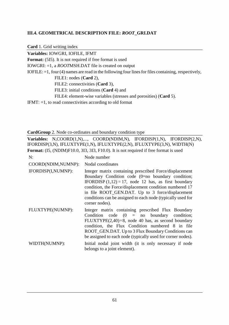
61
III.4. GEOMETRICAL DESCRIPTION FILE: ROOT_GRI.DAT
Card 1. Grid writing index
Variables: IOWGRI, IOFILE, IFMT
Format: (5I5). It is not required if free format is used
IOWGRI: =1, a ROOTMSH.DAT file is created on output
IOFILE: =1, four (4) names are read in the following four lines for files containing, respectively,
FILE1: nodes (Card 2),
FILE2: connectivities (Card 3),
FILE3: initial conditions (Card 4) and
FILE4: element-wise variables (stresses and porosities) (Card 5).
IFMT: =1, to read connectivities according to old format
CardGroup 2. Node co-ordinates and boundary condition type
Variables: N,COORD(1,N),..., COORD(NDIM,N), IFORDISP(1,N), IFORDISP(2,N),
IFORDISP(3,N), IFLUXTYPE(1,N), IFLUXTYPE(2,N), IFLUXTYPE(3,N), WIDTH(N)
Format: (I5, (NDIM)F10.0, 3I3, 3I3, F10.0). It is not required if free format is used
N: Node number
COORD(NDIM,NUMNP): Nodal coordinates
IFORDISP(I,NUMNP): Integer matrix containing prescribed Force/displacement
Boundary Condition code (0=no boundary condition;
IFORDISP (1,12) = 17, node 12 has, as first boundary
condition, the Force/displacement condition numbered 17
in file ROOT_GEN.DAT. Up to 3 force/displacement
conditions can be assigned to each node (typically used for
corner nodes).
FLUXTYPE(NUMNP): Integer matrix containing prescribed Flux Boundary
Condition code (0 = no boundary condition;
FLUXTYPE(2,40) = 8, node 40 has, as second boundary
condition, the Flux Condition numbered 8 in file
ROOT_GEN.DAT. Up to 3 Flux Boundary Conditions can
be assigned to each node (typically used for corner nodes).
WIDTH(NUMNP): Initial nodal joint width (it is only necessary if node
belongs to a joint element).

62
CardGroup 3. Node connectivities, material, element type, ...
Variables: L, MTYPE, LTYPE, KXX(1,L), ..., KXX(MNNEL,L)
Format: ((3+MNNEL)I5). It is not required if free format is used
L: Element number
MTYPE(L): Material type
LTYPE(L): Element type
KXX(MNNEL,L): Global conectivities (the maximum number of connectivities
is 2 (ndim=1), 6 (ndim=2), and 8 (ndim=3),
MNNEL is the maximum number of nodes that may have a possible element in the finite
element grid that is used in a problem. With the elements that are implemented at present the
following values are internally assigned to MNNEL: for NDIM=1 is MNNEL=2, for NDIM=2
is MNNEL=6, and for NDIM=3 is MNNEL=8.
CardGroup 4. Initial values of unknowns
Variables: N, X(1,N), ..., X(NDF, N)
Format: (I5, 10F15.0). It is not required if free format is used
N: Node number
X: Array containing old values of unknowns
Here, the initial values of the unknowns are read and stored as the OLD values to begin time
marching calculations.
In general, the following variables should be read:
n ux uy uz Pl Pg T
I5 F15.0 F15.0 F15.0 F15.0 F15.0 F15.0
CardGroup 5. Initial values of stresses
Variables: L, STRESS(1,L), ..., STRESS(6,L) , HISTVAR(1,L), HISTVAR(2,L)
Format: (I5, 10F15.0). It is not required if free format is used
(Omit if IOPTDISPL = 0)
L: Element number
STRESS: Array containing the stress tensor at integration points (if the element uses several
integration points, only 1 value per element is read and assumed initially the same
in all integration points)
HISTVAR: Array containing history variables for elastoplastic and viscoplastic models

63
CardGroup 6. Other element wise properties.
Variables: L, POROSITY(L), (FK(I,L),I=1,NDIM), ANISOTPER(1,
L), ..., ANISOTPER(NISOT, L), THICKNESS (L), (FK(I, L), I=NDIM+1,NDIM+3)
Format: (I5, 10F15.0). It is not required if free format is used
L: Element number.
POROSITY(L): Initial porosity of element L
FK(I,L): Element-wise multiplying factor for intrinsic permeability
ANISOTPER(1,L): Angle of direction of anisotropy
ANISOTPER(NISOT,L): (NISOT =1 for NDIM=1 OR 2 ; NISOT =3 for NDIM=3)
THICKNESS (L): (only for segment in 2-D or 3-D, LTYPE=8)
FK(I,L): Element-wise multiplying factor for retention curve
parameters
Card 7. Time evolution of state or dependent variables at nodes
Variables: NOUTOT, IVOU(1), ..., IVOU(10), INTERNODE
Format: (16I5). It is not required if free format is used
NOUTOT: Number of nodes for which time evolution is required
IVOU: Variable required at these nodes. IVOU can range from 1 (first
unknown) to NDF (last unknown), and from NDF+1 (first nodal
dependent variable (DEPVARN vector)) to NDF+NDVN (last nodal
dependent variable).
INTERNODE: Frequency for output (=1 implies all time steps).
Card 8. Nodes for time evolution
Variables: NODOUT(1), ..., NODOUT(NOUTOT)
Format: (16I5). It is not required if free format is used
NODOUT(1,..,10): Node number of nodes for which time evolution is required. Time
evolution is written at file 'FOR050.DAT' for time steps according
to INTERNODE.
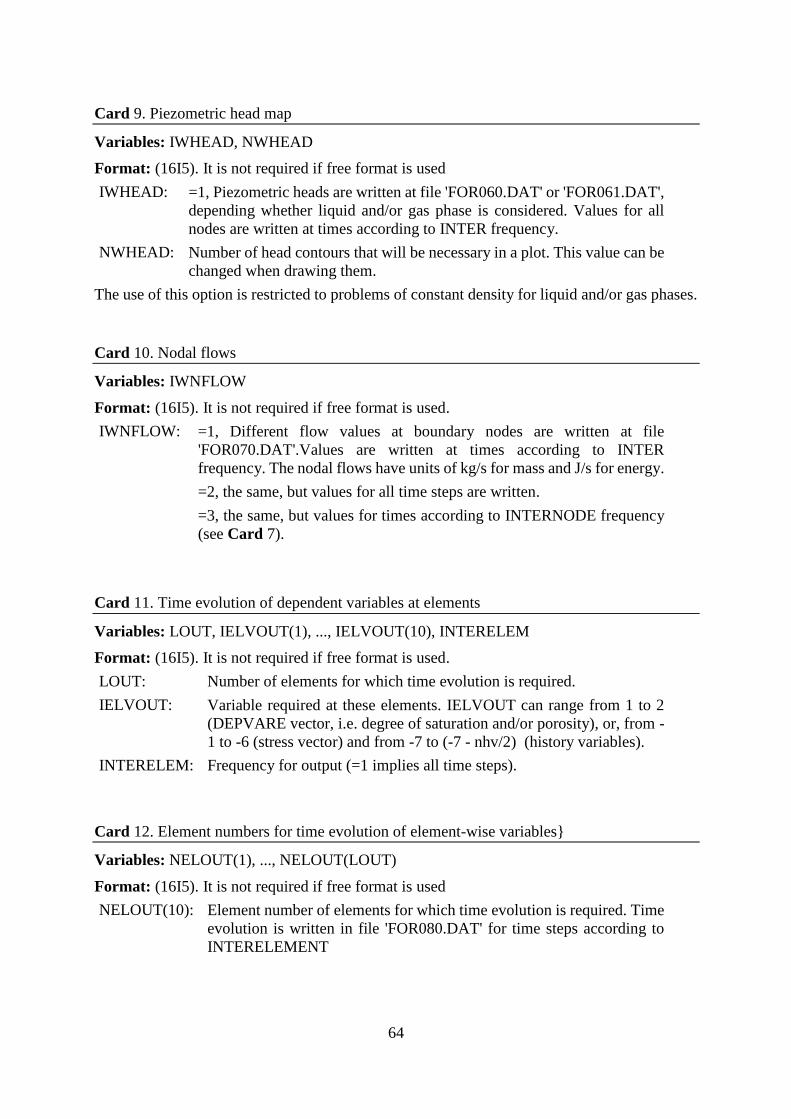
64
Card 9. Piezometric head map
Variables: IWHEAD, NWHEAD
Format: (16I5). It is not required if free format is used
IWHEAD: =1, Piezometric heads are written at file 'FOR060.DAT' or 'FOR061.DAT',
depending whether liquid and/or gas phase is considered. Values for all
nodes are written at times according to INTER frequency.
NWHEAD: Number of head contours that will be necessary in a plot. This value can be
changed when drawing them.
The use of this option is restricted to problems of constant density for liquid and/or gas phases.
Card 10. Nodal flows
Variables: IWNFLOW
Format: (16I5). It is not required if free format is used.
IWNFLOW: =1, Different flow values at boundary nodes are written at file
'FOR070.DAT'.Values are written at times according to INTER
frequency. The nodal flows have units of kg/s for mass and J/s for energy.
=2, the same, but values for all time steps are written.
=3, the same, but values for times according to INTERNODE frequency
(see Card 7).
Card 11. Time evolution of dependent variables at elements
Variables: LOUT, IELVOUT(1), ..., IELVOUT(10), INTERELEM
Format: (16I5). It is not required if free format is used.
LOUT: Number of elements for which time evolution is required.
IELVOUT: Variable required at these elements. IELVOUT can range from 1 to 2
(DEPVARE vector, i.e. degree of saturation and/or porosity), or, from -
1 to -6 (stress vector) and from -7 to (-7 - nhv/2) (history variables).
INTERELEM: Frequency for output (=1 implies all time steps).
Card 12. Element numbers for time evolution of element-wise variables}
Variables: NELOUT(1), ..., NELOUT(LOUT)
Format: (16I5). It is not required if free format is used
NELOUT(10): Element number of elements for which time evolution is required. Time
evolution is written in file 'FOR080.DAT' for time steps according to
INTERELEMENT
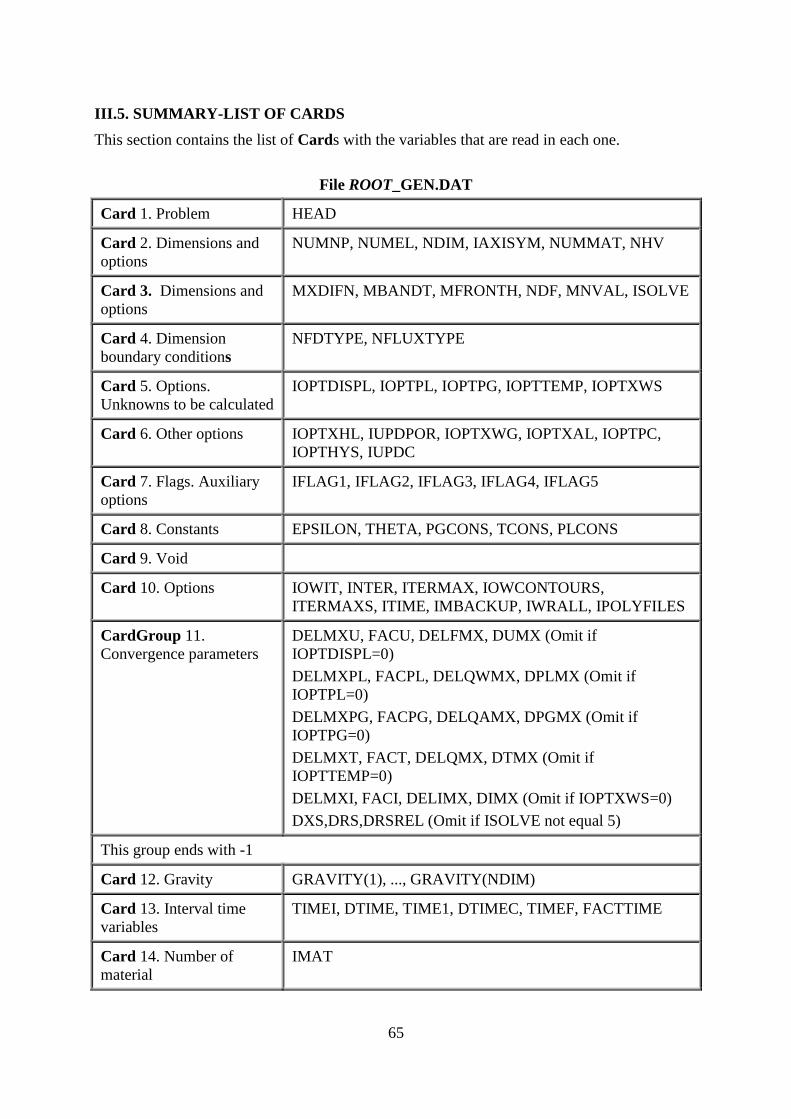
65
III.5. SUMMARY-LIST OF CARDS
This section contains the list of Cards with the variables that are read in each one.
File ROOT_GEN.DAT
Card 1. Problem HEAD
Card 2. Dimensions and
options
NUMNP, NUMEL, NDIM, IAXISYM, NUMMAT, NHV
Card 3. Dimensions and
options
MXDIFN, MBANDT, MFRONTH, NDF, MNVAL, ISOLVE
Card 4. Dimension
boundary conditions
NFDTYPE, NFLUXTYPE
Card 5. Options.
Unknowns to be calculated
IOPTDISPL, IOPTPL, IOPTPG, IOPTTEMP, IOPTXWS
Card 6. Other options IOPTXHL, IUPDPOR, IOPTXWG, IOPTXAL, IOPTPC,
IOPTHYS, IUPDC
Card 7. Flags. Auxiliary
options
IFLAG1, IFLAG2, IFLAG3, IFLAG4, IFLAG5
Card 8. Constants EPSILON, THETA, PGCONS, TCONS, PLCONS
Card 9. Void
Card 10. Options IOWIT, INTER, ITERMAX, IOWCONTOURS,
ITERMAXS, ITIME, IMBACKUP, IWRALL, IPOLYFILES
CardGroup 11.
Convergence parameters
DELMXU, FACU, DELFMX, DUMX (Omit if
IOPTDISPL=0)
DELMXPL, FACPL, DELQWMX, DPLMX (Omit if
IOPTPL=0)
DELMXPG, FACPG, DELQAMX, DPGMX (Omit if
IOPTPG=0)
DELMXT, FACT, DELQMX, DTMX (Omit if
IOPTTEMP=0)
DELMXI, FACI, DELIMX, DIMX (Omit if IOPTXWS=0)
DXS,DRS,DRSREL (Omit if ISOLVE not equal 5)
This group ends with -1
Card 12. Gravity GRAVITY(1), ..., GRAVITY(NDIM)
Card 13. Interval time
variables
TIMEI, DTIME, TIME1, DTIMEC, TIMEF, FACTTIME
Card 14. Number of
material
IMAT

66
Card 15. Number and
name of constitutive law
ICL, TIT, ITYCL
CardGroup 16.
Parameters constitutive
law
TIT, PARCL(1,ICL,IMAT) TIT, PARCL(6,ICL,IMAT)
TIT, PARCL(2,ICL,IMAT) TIT, PARCL(7,ICL,IMAT)
TIT, PARCL(3,ICL,IMAT) TIT, PARCL(8,ICL,IMAT)
TIT, PARCL(4,ICL,IMAT) TIT, PARCL(9,ICL,IMAT)
TIT, PARCL(5,ICL,IMAT) TIT, PARCL(10,ICL,IMAT)
(group of Cards from IMAT=1 to NUMMAT and for every IMAT value from ICL=1 to
NCL (not all ICL are required) )
This group ends with -1 (ICL loop)
This group ends with -1 (IMAT loop)
Card 17. Type of
boundary condition
(Mechanical problem)
IF
CardGroup
18.Force/displacement
prescribed
TIT, FORDISP(1,IF)
TIT, FORDISP(2,IF)
TIT, FORDISP(...,IF)
(group of Cards from IF=1 to NFDTYPE ) (Omit if IOPTDISPL=0)
This group ends with -1
Card 19. Type of
boundary condition. Mass
or heat transport problems
IF
CardGroup 20. Flux
problem boundary
condition
TIT, FLUX(1,IF), TIT, FLUX(21,IF)
TIT, FLUX(2,IF), TIT, FLUX(22,IF)
TIT, FLUX(...,IF, TIT, FLUX(...,IF))
TIT, FLUX(20,IF), TIT, FLUX(40,IF)
(group of Cards from IF=1 to NFLUXTYPE ) (Omit if IOPTPL + IOPTPG +IOPTTEMP =
0)
This group ends with –1
The group of Cards from 13 to 20 can be repeated in order to make a simulation with several
time intervals in which the boundary conditions and material properties are not the same. If any
parameter is not read, the value in the previous interval is used. If a '-1' is read with IMAT, ICL
and IF, then no change takes place in material properties and boundary conditions.

67
File ROOT_GRI.DAT
Card 1. Grid writing index IOWGRI, IOFILE, IFMT
CardGroup 2. Node co-
ordinates and boundary
condition type
N, COORD(1, N), ..., COORD(NDIM, N), IFORDISP(1,N),
IFORDISP(2,N), IFORDISP(3,N), IFLUXTYPE(1,N),
IFLUXTYPE(2,N), IFLUXTYPE(3,N), WIDTH(N)
(group of Cards from N=1 to NUMNP)
CardGroup 3. Node
connectivities, material,
element type,...
L, MTYPE, LTYPE, KXX(1,L),..., KXX(MNNEL,L)
(group of Cards with L=1 to NUMEL)
CardGroup 4. Initial
values of unknowns
N, XOLD(1,N), ..., XOLD(NDF,N)
(group of Cards with N=1 to NUMNP)
CardGroup 5. Initial
values of stresses
L, STRESSOLD(1, 1, L), ..., STRESSOLD(NSTREC, 1, L)
(group of Cards with L=1 to NUMEL) (Omit if IOPTDISPL=0)
CardGroup 6. Other
element wise properties
L, POROSITY(L), (FK(I, L), I=1,NDIM), ANISOTPER(1,
L), ..., ANISOTPER(NISOT, L), THICKNESS (L),
(FK(I,L), I=NDIM+1, NDIM+3)
(group of Cards with L=1 to NUMEL)
Card 7. Time evolution of
state or dependent variables
at nodes
NOUTOT, IVOU(1), ..., IVOU(10), INTERNODE
Card 8. Nodes for time
evolution
NODOUT(1), ..., NODOUT(NOUTOT)
Card 9. Piezometric head
map
IWHEAD, NWHEAD
Card 10. Nodal flows IWNFLOW
Card 11. Time evolution of
dependent variables at
elements
LOUT, IELVOUT(1), ..., IELVOUT(10),
INTERELEMENT
Card 12. Element numbers
for time evolution of
element-wise variables
NELOUT(1), ..., NELOUT(LOUT)
_________________________________

68
IV. CODE_BRIGHT. POSTPROCESS.
IV.1. POST-PROCESSING TOOLS: SHORT DESCRIPTION
The different results that the system allows to display are the following ones:
Geometry: GiD displays the whole volumetric mesh, surface sets and boundary surfaces. It
can also cut and divide them, in its original state as well as also in its deformed state, and
switch them on and off. GiD displays how the meshes/sets will be deformed according to a
certain vectorial variable. GiD provides two representations: on the first one all the results
will then be drawn on these original or deformed meshes (Main Geometry); on the second
one, a superimposed representation (Show Geometry) is provided, that can be also deformed,
but the results will still be drawn on the main representation. The user can compare the main
original/deformed meshes/sets with the second representation, which can also be deformed
with the same or another vector deformation, or with no deformation at all. The scaling of
all the displays can be modified interactively.
Show minimum and maximum: The minimum and maximum values of the variable for
the currently viewed meshes/sets can appear, pointing all the nodes where these limits are
computed, in dark blue the minimum values and in red the maximum ones.
Vectors: GiD presents a vector distribution according to the vectorial or matrix variables on
each node, showing their magnitudes and directions. The scaling of the vectors can be
modified interactively.
Contour fields: GiD represents the variables through isosurfaces or contours that comprise
all the values between two given values. GiD takes advantage of the graphical capabilities
of the machine, allowing a smoothing of the results when a high number of colors is used.
Contour lines: This representation is quite similar to the last one, but the uniform bands are
substituted here by isolines, where each one ties several points with the same value.
IV.2. READ POST-PROCESSING
GiD displays a ̀ File Open Dialog Box' and asks the user for a file. Afterwards, it looks
for the files filename.msh, filename.bon and filename.res. The description of
what is found and being read, sorted (if necessary) and built appears on the message bar.
Sometimes, it may be useful to use the visualization options to center and zoom the drawing on
the screen, especially when the different scales affect the post-processing. All the post-
processing facilities can be used for this new project, jump to the pre-processing, if desired, or
go back to the previous or another project post-processings.
Other details on post-processing information are available from the GiD manual.
IV.3. POST PROCESS FILES FORMAT
In some cases the user needs to interact with the results given by the CODE_BRIGHT process
in order to obtain different variables that are function of the variables considered as a result.
The information needed to do that is stored in the post-process files, which are saved in the
work directory. These files are:
root.post.res
root.post.msh

69
The file root.post.msh contains information about the mesh, like the coordinates of the nodes,
and the coordinates of the elements, while the file root.post.res presents the information of the
results and the variation in time of different variables in the nodes or Gauss points. To create
the program it is important to take into account the format of these files, specially the
root.pos.res file. Note that with root we mean the root name of the project: for example, if our
project is DAM.gid then the post process files will be DAM.post.res and DAM.post.msh.
The first lines of the file root.pos.res are the header, which contains information about the Gauss
points. Based on the type of element employed, this header may have 5 or 10 lines: 5 lines for
triangular elements and 10 lines for quadrilateral elements. See Figure IV.3.1.
Header for quadrilateral elements
Header for triangular elements
Figure IV.3.1. Header format for quadrilateral and triangular elements
The results of the process appear in the next lines. The results are divided by time, which means
that are presented for variable 1 in time 1, then variable 2 in time 1, until the last variable, and
then start again for all the variables in time 2 and so on.
The line 6 −or 11, depending on the element employed− presents the header for the results of
variable 1 in time 1, which has the following format:
Result “Variable” Isochrones “time” “type” “set”
Variable: Ex. Temperature, liquid pressure, stress
Type: Vector, scalar or matrix.
Set: Nodes (onNodes) or Gauss points (GP) depending of the variable.
For example: Result Temperature Isochrones 0.549584E-06 Scalar onNodes
The next line has the text “Values”. In the following lines 2 columns for scalar type variables
appear, 3 columns for variable type vector or 6 columns for matrix type, as it is shown in Figure
IV.3.2. The first column presents the number of the node or Gauss point, whose coordinates are
presented in the file root.post.msh. After the last value, the line “end values” appears and in the
succeeding line the header for the next variable appears.

70
Result format for a scalar variable.
Result format for a vector variable.
Result format for a matrix variable.
Figure IV.3.2. Results
If the user needs to create another file type root.post.res to visualize the results in the GID
interface, it is important to consider the format presented before, and take into account that the
header of the values has the following format:
‘Result’,1x,a15,1x,’Isochrones `,e12.6,1x,a15,1x,a30

71
V. CODE_BRIGHT. THEORETICAL ASPECTS
In porous media, subjected to thermal, hydraulic, and mechanical conditions, relevant thermo-
hydro-mechanical (THM) phenomena takes place. In fact, there exist a number of mutual
interactions that must be taken simultaneously into account in analyses. For instance, strains
due to thermal loading will induce stress variations and changes in mass storage terms and
hydraulic conductivity. The thermal expansion of the water in the pores itself causes changes
in the degree of saturation or, if the material is saturated or quasi-saturated, increases of water
pressure. Thermal induced vapor diffusion and the dependence of water viscosity on
temperature also affect significantly the water transfer process.
On the other hand, changes in hydraulic conditions influence the temperature field via variations
of thermal conductivity and affect the stress/strain field due to pore water pressure and pore gas
pressure changes. Gas pressure is affected by the increase in vapour pressure with temperature.
This may lead to further changes in the pattern of gas and water flow. Finally, porosity changes
due to volumetric strain influence pore pressure distributions because of associated variations
in storage terms and hydraulic conductivity. The effect on temperature is less important as the
variations of thermal conductivity with porosity are relatively small. In Appendix 1 the most
significant interactions between the various phenomena are presented in a systematic manner.
An unavoidable consequence of all those phenomena interacting simultaneously is the need to
carry out coupled THM analysis in which all the main aspects of the problem can be considered
in an integrated way. Such a formulation and the numerical approach adopted to solve the
governing equations are presented in the following sections.
V.1. BASIC FORMULATION FEATURES
A porous medium composed by solid grains, water and gas is considered. Thermal, hydraulic
and mechanical aspects will be taken into account, including coupling between them in all
possible directions. As illustrated in Figure V.1.1, the problem is formulated in a multiphase
and multispecies approach.
Gas phase: dry air + water
vapour
Solid phase
Liquid phase:
water +
dissolved air
Figure V.1.1. Schematic representation of an unsaturated porous material

72
The three phases are:
solid phase (s) : mineral
liquid phase (l) : water + air dissolved
gas phase (g) : mixture of dry air and water vapour
The three species are:
solid (-) : the mineral is coincident with solid phase
water (w) : as liquid or evaporated in the gas phase
air (a) : dry air, as gas or dissolved in the liquid phase
The following assumptions and aspects are taken into account in the formulation of the problem:
Dry air is considered a single species and it is the main component of the gaseous
phase. Henry's law is used to express equilibrium of dissolved air.
Thermal equilibrium between phases is assumed. This means that the three phases are
at the same temperature
Vapour concentration is in equilibrium with the liquid phase. Psychrometric law
expresses its concentration.
State variables (also called unknowns) are: solid displacements, u (three spatial
directions); liquid pressure, Pl; gas pressure, Pg; and temperature, T.
Balance of momentum for the medium as a whole is reduced to the equation of stress
equilibrium together with a mechanical constitutive model to relate stresses with
strains. Strains are defined in terms of displacements.
Small strains and small strain rates are assumed for solid deformation. Advective terms
due to solid displacement are neglected after the formulation is transformed in terms
of material derivatives (in fact, material derivatives are approximated as eulerian time
derivatives). In this way, volumetric strain is properly considered.
Balance of momentum for dissolved species and for fluid phases are reduced to
constitutive equations (Fick's law and Darcy's law).
Physical parameters in constitutive laws are function of pressure and temperature. For
example: concentration of vapour under planar surface (in psychrometric law), surface
tension (in retention curve), dynamic viscosity (in Darcy's law), strongly depend on
temperature.

73
V.2. GOVERNING EQUATIONS
The governing equations for non-isothermal multiphase flow of water and gas through porous
deformable saline media have been presented by Olivella et al. (1994). A detailed derivation is
given there, and only a brief description is included here.
The equations that govern this problem can be categorised into four main groups. These are:
balance equations, constitutive equations, equilibrium relationships and definition constraints.
Equations for mass balance were established following the compositional approach. That is,
mass balance is performed for water, air and salt species instead of using solid, liquid and gas
phases. Equation for balance of energy is established for the medium as a whole. The equation
of momentum balance for the porous medium is reduced to that of stress equilibrium.
The following notation will be used in writing balance equations:
𝜙: porosity b: body forces,
𝜌: density 𝜔: mass fraction,
𝐣: total mass flux 𝜌: mass content per unit volume of phase,
𝐢: non-advective mass flux e: specific internal energy
𝐪: advective flux 𝐢𝒄: conductive heat flux
𝐮: solid displacements 𝐣𝑒: energy fluxes due to mass motion
𝛔: stress tensor
𝑆𝑙, 𝑆𝑔: degree of saturation of liquid and gaseous phases i.e., fraction of pore volume occupied
by each phase.
Superscripts w and a refer to water and air, respectively
Subscripts s, l and g refer to solid, liquid and gas phase, respectively.
V.2.1. Balance Equations
The compositional approach is adopted to establish the mass balance equations. Volumetric
mass of a species in a phase (e.g. water in gas phase 𝜌𝑔𝑤 is the product of the mass fraction of
that species (𝜔𝑔𝑤) and the bulk density of the phase (𝜌𝑔), i.e. 𝜌𝑔
𝑤 = 𝜔𝑔𝑤𝜌𝑔.
The total mass flux of a species in a phase (e.g. flux of air present in gas phase 𝐣𝑔𝑤 is, in general,
the sum of three terms:
the nonadvective flux: 𝐢𝑔𝑤, i.e. diffusive/ dispersive,
the advective flux caused by fluid motion: 𝜔𝑔𝑤𝜌𝑔𝐪𝑔, where 𝐪𝑔 is the Darcy's flux,
the advective flux caused by solid motion: 𝜔𝑔𝑤𝜌𝑔𝑆𝑔𝜙
𝑑𝒖
𝑑𝑡 where
𝑑𝒖
𝑑𝑡 is the vector of solid
velocities, 𝑆𝑔 is the volumetric fraction of pores occupied by the gas phase and 𝜙 is
porosity.
The sum of the nonadvective and fluid motion advective fluxes is separated from the total flux
in order to simplify algebraic equations. This flux is relative to the solid phase and is denoted
by 𝐣′𝑔𝑤. It corresponds to the total flux minus the advective part caused by solid motion. When
solid deformation is negligible, then j’ = j. The relative contribution of each flux term to the
total flux is not always the same. For instance, diffusion will become more important if
advection is small.

74
Mass balance of solid
Mass balance of solid present in the medium is written as:
𝜕(𝜌𝑠(1 − 𝜙))
𝜕𝑡+ ∇ ∙ (𝐣𝑠) = 0
(1)
where s is the mass of solid per unit volume of solid and js is the flux of solid. From this
equation, an expression for porosity variation was obtained as:
𝐷𝑠𝜙
𝐷𝑡=(1 − 𝜙)
𝜌𝑠
𝐷𝑠𝜌𝑠𝐷𝑡
+ (1 − 𝜙)∇ ∙𝑑𝐮
𝑑𝑡
(2)
The material derivative with respect to the solid has been used and its definition is:
𝐷𝑠(∎)
𝐷𝑡=𝜕(∎)
𝜕𝑡+𝑑𝐮
𝑑𝑡∙ ∇(∎)
(3)
Equation (2) expresses the variation of porosity caused by volumetric deformation and solid
density variation.
Mass balance of water
Water is present in liquid and gas phases. The total mass balance of water is expressed as:
𝜕 ((𝜔𝑔𝑤𝜌𝑔 𝑆𝑔 + 𝜔𝑙
𝑤𝜌𝑙 𝑆𝑙)𝜙)
𝜕𝑡+ 𝛻 ∙ (𝐣𝑔
𝑤 + 𝐣𝑙𝑤) = 𝑓𝑤
(4)
where f w is an external supply of water. An internal production term is not included because
the total mass balance inside the medium is performed. The use of the material derivative leads
to:
𝜙𝐷𝑠(𝜔𝑙
𝑤𝜌𝑙 𝑆𝑙 + 𝜔𝑔𝑤𝜌𝑔 𝑆𝑔)
𝐷𝑡+ (𝜔𝑙
𝑤𝜌𝑙 𝑆𝑙 + 𝜔𝑔𝑤𝜌𝑔 𝑆𝑔)
𝐷𝑠𝜙
𝐷𝑡+
+(𝜔𝑙𝑤𝜌𝑙 𝑆𝑙 + 𝜔𝑔
𝑤𝜌𝑔 𝑆𝑔)𝜙𝛻 ∙𝑑𝐮
𝑑𝑡+ 𝛻 ∙ (𝐣𝑙
′𝑤 + 𝐣𝑔′𝑤) = 𝑓𝑤
(5)
The final objective is to find the unknowns from the governing equations. Therefore, the
dependent variables will have to be related to the unknowns in some way. For example, degree
of saturation will be computed using a retention curve which should express it in terms of
temperature, liquid pressure and gas pressure.
Porosity appears in this equation of water mass balance not only as a coefficient, but also in a
term involving its variation caused by different processes. It is also hidden in variables that
depend on porosity (e.g. intrinsic permeability). The way of expressing the derivative term as a
function of the state variables is via the solid mass balance equation. This allows to take into
account correctly the influence of porosity variation in the balance equation for water.
It should be noted that in the last equation the material derivatives can be approximated as
eulerian if the assumption of small strain rate is performed while the volumetric change
(porosity derivative and volumetric strain) is not neglected. This is the classical way of
obtaining the coupled flow-deformation equations.

75
Mass balance of air
Once the other mass balance equations have been written it is straightforward to obtain the mass
balance of air taking into account that air is the main component of the gas phase and that it
may be also present as air dissolved in the liquid phase.
𝜙𝐷𝑠(𝜔𝑙
𝑎𝜌𝑙 𝑆𝑙 + 𝜔𝑔𝑎𝜌𝑔 𝑆𝑔)
𝐷𝑡+ (𝜔𝑙
𝑎𝜌𝑙 𝑆𝑙 + 𝜔𝑔𝑎𝜌𝑔 𝑆𝑔)
𝐷𝑠𝜙
𝐷𝑡+
+(𝜔𝑙𝑎𝜌𝑙 𝑆𝑙 + 𝜔𝑔
𝑎𝜌𝑔 𝑆𝑔)𝜙𝛻 ∙𝑑𝐮
𝑑𝑡+ 𝛻 ∙ (𝐣𝑙
′𝑎 + 𝐣𝑔′𝑎) = 𝑓𝑎
(6)
Momentum balance for the medium
The momentum balance reduces to the equilibrium of stresses if the inertial terms are neglected:
b 0 (7)
where is the stress tensor and b is the vector of body forces.
Internal energy balance for the medium
The equation for internal energy balance for the porous medium is established taking into
account the internal energy in each phase (es, el, eg) or enthalpy (hs, hl, hg):
𝜕(𝑒𝑔𝜌𝑠 (1 − 𝜙) + 𝑒𝑔𝜌𝑔 𝑆𝑔𝜙 + 𝑒𝑙𝜌𝑙 𝑆𝑙𝜙)
𝜕𝑡−𝜙𝑆𝑔𝑝𝑔
𝜌𝑔
𝜕𝜌𝑔
𝜕𝑡+
+𝛻 ∙ (𝐢𝑐 + 𝐣𝑒𝑠 + 𝐣𝑒𝑔 + 𝐣𝑒𝑙) = 𝑓𝑄
𝜕(ℎ𝑠𝜌𝑠 (1 − 𝜙) + ℎ𝑔𝜌𝑔 𝑆𝑔𝜙 + ℎ𝑙𝜌𝑙 𝑆𝑙𝜙)
𝜕𝑡− 𝜙𝑆𝑔
𝜕𝑝𝑔
𝜕𝑡+
+𝛻 ∙ (𝐢𝑐 + 𝐣ℎ𝑠 + 𝐣ℎ𝑔 + 𝐣ℎ𝑙) = 𝑓𝑄
(8)
where 𝐢𝑐 is energy flux due to conduction through the porous medium, the other fluxes (𝐣𝑒𝑠, 𝐣𝑒𝑙,
𝐣𝑒𝑔, 𝐣ℎ𝑠, 𝐣ℎ𝑙, 𝐣ℎ𝑔) are advective fluxes of energy or enthalpy caused by mass motions and 𝑓𝑄 is
an internal/external energy supply (heat supply). In this case this term accounts, for instance,
energy dissipation due to medium deformation which is not explicit because it is negligible in
most cases. The use of the material derivative allows obtaining an equation formally similar to
the mass balance of water. The reason for the similarity is that both water and internal energy,
are considered present in the three phases.
Hence, only one equation is required which expresses the balance of internal energy in the
porous medium as a whole. The enthalpy equation is obtained using the definition of enthalpy
as ℎ = 𝑒 + 𝑝𝑣. The density time derivative or the pressure time derivative terms in energy or
enthalpy balance are sometimes neglected.
The fluxes in the divergence term include conduction of heat and advection of heat caused by
the motion of every species in the medium. A non-advective mass flux causes an advective heat

76
flux because a species inside a phase moves and transports energy. Contrary to what happens
with the movement of a contaminant in a groundwater system, the diffusive term for heat
transport (conduction of heat) is much larger than the term concerning hydromechanical
dispersion (non-advective flux caused by the velocity of fluids). For this reason, this term is
sometimes neglected.
V.2.2. Constitutive equations and equilibrium restrictions
Associated with this formulation there is a set of necessary constitutive and equilibrium laws.
Table V.2.1 is a summary of the constitutive laws and equilibrium restrictions that should be
incorporated in the general formulation. The dependent variables that are computed using each
of the laws are also included.
Table V.2.1. Constitutive equations and equilibrium restrictions
EQUATION VARIABLE NAME VARIABLE
Constitutive equations
Darcy's law liquid and gas advective flux 𝐪𝑙, 𝐪𝑔
Fick's law vapour and air non-advective fluxes 𝐢𝑔𝑤, 𝐢𝑙
𝑎
Fourier's law conductive heat flux 𝐢𝒄
Retention curve Liquid phase degree of saturation 𝑆𝑙, 𝑆𝑔
Mechanical constitutive model Stress tensor 𝛔
Phase density liquid density 𝜌𝑙
Gases law gas density 𝜌𝑔
Equilibrium restrictions
Henry's law Air dissolved mass fraction 𝜔𝑙𝑎
Psychrometric law Vapour mass fraction 𝜔𝑔𝑤
The constitutive equations establish the link between the independent variables (or unknowns)
and the dependent variables. There are several categories of dependent variables depending on
the complexity with which they are related to the unknowns. The governing equations are
finally written in terms of the unknowns when the constitutive equations are substituted in the
balance equations.
Another type of relationships that relate dependent variables with unknowns are the equilibrium
restrictions. They are obtained assuming chemical equilibrium for dissolution of the different
species (air and vapour) in phases (liquid, gas). This assumption is sufficiently adequate
because these chemical processes are fast compared to the transport processes that take place
in porous media and, for this reason, they are not rate controlling.

77
V.2.3. Boundary conditions
Application of the Green's theorem to the divergence term (both in the balance or equilibrium
of stresses equations) produces terms which represent fluxes or stresses across or on the
boundaries. These terms are substituted by nodal flow rates or forces in the discretized form of
the equations. For the mechanical problem, the classical approach is followed to impose
external forces. Imposing displacements is made by means of a Cauchy type boundary
condition, i.e. a force computed as the stiffness of a spring times the displacement increment.
The boundary conditions for balance equations are incorporated by means the simple addition
of nodal flow rates. For instance, the mass flow rate of water as a component of gas phase (i.e.
vapour) is:
j j P Pg
w
g
w
g g
w
g g g g g g
w
g g
w
00
00
0
(9)
where the superscript ()0 stands for prescribed values. This general form of boundary condition,
includes three terms. The first one is the mass inflow or outflow that takes place when a flow
rate of gas (jg0) is prescribed. The second term is the mass inflow or outflow that takes place
when the gas phase pressure (Pg0) is prescribed at a node. The coefficient g is a leakage
coefficient, i.e., a parameter that allows a boundary condition of the Cauchy type. The third
term is the mass inflow or outflow that takes place when vapour mass fraction is prescribed at
the boundary. This term naturally comes from the nonadvective flux (Fick's law). Mass fraction
and density prescribed values are only required when inflow takes place. For outflow, the values
in the medium are considered. For the energy balance equation, the boundary condition has a
similar form.
V.2.4. Summary of governing equations
As stated above the governing equations for non-isothermal multiphase flow of liquid and gas
through porous deformable saline media have been established by Olivella et al. (1994). A
detailed derivation is presented there. The theoretical work briefly presented above has been
used as a basis for the development of the computer program CODE_BRIGHT, which stands
for COupled DEformation, BRIne, Gas and Heat Transport problems.
Table V.2.2.: Equation and variable summary
EQUATION VARIABLE NAME VARIABLE
equilibrium of stresses displacements u
balance of water mass liquid pressure Pl
balance of air mass gas pressure Pg
balance of internal energy temperature T

78
V.3. NUMERICAL APPROACH
V.3.1. Introduction
The system of PDE's (Partial Differential Equations) is solved numerically. The numerical
approach can be viewed as divided into two parts: spatial and temporal discretizations. Finite
element method is used for the spatial discretization while finite differences are used for the
temporal discretization. The discretization in time is linear and the implicit scheme uses two
intermediate points, tk+ and tk+ between the initial tk and final tk+1 times. Finally, since the
problem presented here is non-linear, the Newton-Raphson method was adopted to find an
iterative scheme.
Figure V.3.1. Concept of cell in a finite element mesh.
Once the solid balance is substituted in the other balance equations, computation of porosity at
an intermediate point is not necessary because its variation is expected to occur at slow rates.
For this reason, porosity is integrated explicitly, that is, the values at tk are used. Since the
variation of porosity is expressed by the solid mass balance equation, this assumption leads also
to some advantages for the iterative scheme. After the spatial discretization of the partial
differential equations, the residuals that are obtained can be written (for one finite element) as:
r
r
r
r
d
d
d
d
a
a
a
a
b
b
b
b
0
0
0
0
u
P
P
T
u
P
P
T
u
P
P
T
u
P
P
T
l
g
l
g
l
g
l
g
d
dt
(10)
where r are the residuals, dd/dt are the storage or accumulation terms, a are the conductance
terms, and b are the sink/source terms and boundary conditions. After time discretization a more
compact form can read as:
r Xd d
A X X b X 0( ) ( ) ( )k
k k
k
k k k
t
1
1
(11)
j k
i
em
en

79
where k is the time step index, : X=[(ux,uy,uz,Pl,Pg,T)(1), ..., (ux,uy,uz,Pl,Pg,T)(n)], is the vector of
unknowns (i.e. a maximum of seven degrees of freedom per node), A represents the
conductance matrix. The Newton-Raphson scheme of solution for this non-linear system of
AE's is:
r X
XX X R X
( )( ) ( ), , ,
k
k
k l k l k l
1
1
1 1 1 1
(12)
where l indicates iteration.
In the present approach, the standard Galerkin method is used with some variations in order to
facilitate computations. General aspects related to numerical solution of hydrogeological
problems can be found in Huyakorn and Pinder (1983). As shown in the preceding section, in
the mass and energy balance equations the following terms may be distinguished:
Storage terms. These terms represent the variation of mass or energy content and therefore,
they are calculated by means of variables such as degree of saturation, density, porosity,
mass fraction and specific energy.
Advective fluxes. The advective fluxes caused by motion of fluids computed using Darcy's
law and, except for the coefficients, they are explicit in terms of pressure gradients.
Nonadvective fluxes. These terms, computed through Fick's law, are proportional to
gradients of mass fractions which do not belong to the set of unknowns. Fourier's law is used
for the conductive heat flux and it expresses proportionality to temperature gradients.
Volumetric strain terms. In fact, these terms are also storage terms. They are proportional to
du/dt which is equivalent to the volumetric strain rate.
Sink/source terms.
Each of these terms requires specific treatment. This is described in detail in Olivella et al
(1996).
In order to explain the treatment of the different terms and equations the following notation is
introduced:
node i: node in a finite element mesh
e1,e2,...,em: elements that contain node i, i.e. a cell centered in node i is composed by a
fraction of these elements. m is variable from node to node and it is not related to the number
of nodes per element.
nem: number of nodes in element em. For example, nem=3 for triangles, nem=4 for
quadrilaterals, nem=4 for tetrahedrons, etc.
()k: the quantity is computed at time tk of the temporal discretization. The same for tk+1, tk+
or tk+
()em: the quantity is computed in element em. This means at the center of the element or, in
other words, using the average of nodal unknowns.
()i: the quantity is computed in node i as a function of the unknowns in that node. \item--}
()i,em: the quantity is computed in node i but with the material properties corresponding to
element em.
Vem: volume of element em.
i: shape function for node i.

80
V.3.2. Treatment of different terms
Treatment of storage terms
In this sub-section we refer to terms not related to volumetric strain or porosity variation. The
storage or accumulation terms are computed in a mass conservative approach (Allen and
Murphy, 1986; Celia et al., 1990; Milly, 1984). The conservative approach discretizes directly
the accumulation terms while the capacitative approach uses the chain rule to transform time
derivatives in terms of the unknowns. Milly (1984) proposes modifications of the capacitative
approach in order to conserve mass. It seems reasonable that the mass conservative approach
should give a more accurate solution than the capacitative approach.
Mass conservation in time is achieved if the time derivatives are directly approximated by a
finite difference in time. Finite element method for the space discretization conserves mass
(Milly, 1984).
A typical storage term is (from Eq. 5) the variation of water in the gas phase:
𝜙𝐷𝑠(𝜔𝑔
𝑤𝜌𝑔𝑆𝑔)
𝐷𝑡≅ 𝜙
𝜕(𝜔𝑔𝑤𝜌𝑔𝑆𝑔)
𝜕𝑡 (13)
where the material derivative with respect to the solid is approximated as an eulerian derivative
because the small strain rate assumption. The weighted residual method is applied to the
governing equations and, for node i, (13) is transformed into:
∫ 𝑁𝑖𝜙𝜕(𝜔𝑔
𝑤𝜌𝑔𝑆𝑔)
𝜕𝑡𝑑𝑣
𝑣
=∑∫ 𝑁𝑖𝜙𝜕(𝜔𝑔
𝑤𝜌𝑔𝑆𝑔)
𝜕𝑡𝑑𝑣
𝑒𝑚𝑒𝑚
(14)
At this point of the development we assume that porosity is defined element-wise. An element-
wise variable (Voss, 1984) is space-constant over every element, but different from element to
element. We will use emk for porosity in element em at time tk. Similarly, a cell-wise variable
(Voss, 1984) is space constant over the cell centered in the node. It would be very easy to
compute (14) if the time derivative could be computed in a cell-wise way, because one value
would be sufficient for node i and (14) would be transformed into a very simplified form.
However, the degree of saturation is not only a function of nodal unknowns but also of material
properties such as porosity or retention parameters. To overcome this difficulty, the time
derivative in (14) is computed from nodal unknowns but with material properties of every
element in contact with the node. Hence m values are necessary in node i. Obviously if part of
this time derivative is not material dependent (density and concentration are only function of
temperature and pressure) then the corresponding variables are only computed in the node. This
leads to a kind of modified cell-wise variables.
Making use of these approximations, we finally obtain, for example for any integral in (14):
∫ 𝑁𝑖𝜙𝜕(𝜔𝑔
𝑤𝜌𝑔𝑆𝑔)
𝜕𝑡𝑑𝑣
𝑒𝑚
≅ 𝜙𝑒𝑚𝑘 (
(𝜔𝑔𝑤𝜌𝑔𝑆𝑔)𝑖,𝑒𝑚
𝑘+1− (𝜔𝑔
𝑤𝜌𝑔𝑆𝑔)𝑖,𝑒𝑚
𝑘
𝑡𝑘+1 − 𝑡𝑘)∫ 𝑁𝑖𝑑𝑣
𝑒𝑚
(15)
where a simple finite difference is used for the time discretization. This approximation allows
us to make the space integration independently of the physical variables. Therefore,
computation of geometrical coefficients is necessary only once for a given finite element mesh.
The integral of the shape function over an element is equal to Vem/nem for the case of linear
shape functions. These geometrical coefficients are also called influence coefficients. Without
loss of generality, they can be computed either analytically or numerically. Finally, it should be
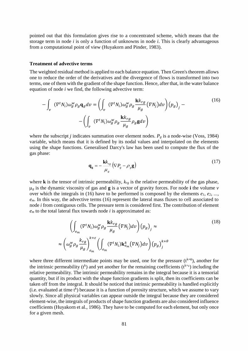
81
pointed out that this formulation gives rise to a concentrated scheme, which means that the
storage term in node i is only a function of unknowns in node i. This is clearly advantageous
from a computational point of view (Huyakorn and Pinder, 1983).
Treatment of advective terms
The weighted residual method is applied to each balance equation. Then Green's theorem allows
one to reduce the order of the derivatives and the divergence of flows is transformed into two
terms, one of them with the gradient of the shape function. Hence, after that, in the water balance
equation of node i we find, the following advective term:
−∫ (𝛻𝑡𝑁𝑖)𝜔𝑔𝑤𝜌𝑔𝐪𝑔𝑑𝑣
𝑣
= (∫ (𝛻𝑡𝑁𝑖)𝜔𝑔𝑤𝜌𝑔
𝐤𝑘𝑟𝑔
𝜇𝑔(𝛻𝑁𝑗)𝑑𝑣
𝑣
) (𝑝𝑔)𝑗−
−(∫ (𝛻𝑡𝑁𝑖)𝜔𝑔𝑤𝜌𝑔
𝐤𝑘𝑟𝑔
𝜇𝑔𝜌𝑔𝐠𝑑𝑣
𝑣
)
(16)
where the subscript j indicates summation over element nodes. Pg is a node-wise (Voss, 1984)
variable, which means that it is defined by its nodal values and interpolated on the elements
using the shape functions. Generalised Darcy's law has been used to compute the flux of the
gas phase:
gk
qg gg
g
rgP
k
(17)
where k is the tensor of intrinsic permeability, krg is the relative permeability of the gas phase,
g is the dynamic viscosity of gas and g is a vector of gravity forces. For node i the volume v
over which the integrals in (16) have to be performed is composed by the elements e1, e2, ...,
em. In this way, the advective terms (16) represent the lateral mass fluxes to cell associated to
node i from contiguous cells. The pressure term is considered first. The contribution of element
em to the total lateral flux towards node i is approximated as:
(∫ (𝛻𝑡𝑁𝑖)𝜔𝑔𝑤𝜌𝑔
𝐤𝑘𝑟𝑔
𝜇𝑔(𝛻𝑁𝑗)𝑑𝑣
𝑒𝑚
) (𝑝𝑔)𝑗≈
≈ (𝜔𝑔𝑤𝜌𝑔
𝑘𝑟𝑔
𝜇𝑔)𝑒𝑚
𝑘+
(∫ (𝛻𝑡𝑁𝑖)𝐤𝑒𝑚𝑘 (𝛻𝑁𝑗)𝑑𝑣
𝑒𝑚
) (𝑝𝑔)𝑗𝑘+𝜃
(18)
where three different intermediate points may be used, one for the pressure (tk+), another for
the intrinsic permeability (tk) and yet another for the remaining coefficients (tk+) including the
relative permeability. The intrinsic permeability remains in the integral because it is a tensorial
quantity, but if its product with the shape function gradients is split, then its coefficients can be
taken off from the integral. It should be noticed that intrinsic permeability is handled explicitly
(i.e. evaluated at time tk) because it is a function of porosity structure, which we assume to vary
slowly. Since all physical variables can appear outside the integral because they are considered
element-wise, the integrals of products of shape function gradients are also considered influence
coefficients (Huyakorn et al., 1986). They have to be computed for each element, but only once
for a given mesh.

82
A similar approximation is used for the gravity term in (16). Evaluation of density element-
wise is convenient in order to balance correctly pressure gradients with gravity forces at element
level.
Treatment of nonadvective terms (diffusive/dispersive)
In the balance equation of node i we find, typically, the following diffusive term:
−∫ (𝛻𝑡𝑁𝑖)𝐢𝑔𝑑𝑣𝑣
= (∫ (𝛻𝑡𝑁𝑖)𝜙𝜏𝜌𝑔𝑆𝑔𝐷𝑔𝑤𝐈(𝛻𝑁𝑗)𝑑𝑣
𝑣
) (𝜔𝑔𝑤)
𝑗
(19)
where the subscript j indicates summation over the nodes. gw is considered a node-wise
variable. Fick's law has been used to compute the diffusive flux:
w
g
w
ggg DS Iig (20)
where is a tortuosity coefficient, Dgw is the molecular diffusion coefficient which is a function
of temperature and gas pressure and I is the identity matrix. The contribution of element em to
the total lateral diffusive flux towards node i is approximated as:
(∫ (𝛻𝑡𝑁𝑖)𝜙𝜏𝜌𝑔𝑆𝑔𝐷𝑔𝑤𝐈(𝛻𝑁𝑗)𝑑𝑣
𝑒𝑚
) (𝜔𝑔𝑤)
𝑗≈
≈ (𝜙𝜏)𝑒𝑚𝑘 (𝜌𝑔𝑆𝑔𝐷𝑔
𝑤)𝑒𝑚
𝑘+(∫ (𝛻𝑡𝑁𝑖)𝐈(𝛻𝑁𝑗)𝑑𝑣
𝑒𝑚
) (𝜔𝑔𝑤)
𝑗
𝑘+𝜃
(21)
where various time intermediate points have been used similarly to what was explained for the
advective terms. The treatment of these diffusive terms also takes advantage of the fact that the
Newton-Raphson method is used to obtain the iterative scheme. We directly interpolate mass
fractions (e.g. gw) and compute gradients.
The dispersive term is treated in a similar way as the diffusive. In this case dispersivities are
element-wise dependent variables. In principle, the liquid and gas fluxes, used to compute the
dispersion tensor, are also computed element-wise.
Treatment of volumetric strain terms
If equation of balance of solid (2) is substituted in all other balance equations, the variations of
porosity are not explicit in them. In this way porosity only appears as parameter or coefficient
and terms of volumetric strain remain in the balance equations. In equation for node i these
terms are of the type:
∫ 𝑁𝑖𝛼𝛻 ∙𝑑𝐮
𝜕𝑡𝑑𝑣
𝑒𝑚
= ∫ 𝑁𝑖𝛼𝐦𝑡𝐁𝑑𝐮
𝜕𝑡𝑑𝑣
𝑒𝑚
(22)
where is defined from de equations and du/dt is the vector of solid velocities, mt =(1,1,1,0,0,0)
is an auxiliary vector and B is the matrix used in the finite element approach for the mechanical
problem. The coefficients of B are gradients of shape functions (Zienkiewick and Zaylor, 1989).
In (22), du/dt is transformed from a continuous vectorial function to a nodal-discrete vectorial
function, although the same symbol is kept (i.e. ux= Nj uxj},..., where j indicates summation).
Following the same methodology as for the other terms we have approximated the integral
given above. The contribution of element em to cell i is:

83
∫ 𝑁𝑖𝛼𝐦𝑡𝐁𝑑𝐮
𝜕𝑡𝑑𝑣
𝑒𝑚
≈ 𝛼𝑒𝑚𝑘+ [∫ 𝑁𝑖𝐦
𝑡𝐁𝑗𝑑𝑣𝑒𝑚
] (𝐮𝑗𝑘+1 − 𝐮𝑗
𝑘
𝑡𝑘+1 − 𝑡𝑘)
(23)
where j indicates summation over element nodes, u is the vector of nodal displacements and Bj
is the j-submatrix of B.
Treatment of mechanical equilibrium equations
The weighted residual method is applied to the stress equilibrium equation [6] followed by the
Green's theorem. This leads to the equation
v
kkk dv 1110fBr
t (24)
where r(k+1) represents the residual corresponding to the mechanical problem and k+1 is the
stress vector. Matrix B (composed by gradients of shape functions) is defined in such a way
that stress is a vector and not a tensor. The body force terms and the boundary traction terms
are represented together by fk+1. The constitutive model relates stresses with strains, with fluid
pressures and with temperatures at a point in the medium. Only if elasticity is included, the total
strain rate is decomposed in the following way:
𝑑𝛆
𝑑𝑡=𝑑𝜺𝑒
𝑑𝑡= (𝐃𝑒)−1
𝑑𝛔′
𝑑𝑡+ 𝐈𝑎𝑠
𝑑𝑠
𝑑𝑡+ 𝐈𝑎𝑇
𝑑𝑇
𝑑𝑡, 𝐈 or 𝐦
(25)
where De is the elasticity matrix, 𝑎𝑠 and 𝑎𝑇 are coefficients for elastic dilation. ’ is the net
stress tensor defined as ’= + m Pg (compression negative). On the other hand, strain will be
written in terms of displacements because = B u. The last equation (25) must satisfy at every
point in the medium. Space and time discretization lead to:
𝐡𝑘+1 = −𝐃𝑒𝐁(𝐮𝑘+1 − 𝐮𝑘) + (𝛔𝑘+1 − 𝛔𝑘) + 𝐈(𝑝𝑔𝑘+1 − 𝑝𝑔
𝑘) + 𝐃𝑒𝐈𝑎𝑠(𝑠𝑘+1 − 𝑠𝑘)
+ 𝐃𝑒𝐈𝑎𝑇(𝑇𝑘+1 − 𝑇𝑘)
(26)
where h is the residual of stresses at every point. If stress can be obtained in an explicit way
from (26), it is simply substituted in (24). However, when nonlinear models are introduced a
substitution of the differential or incremental forms is necessary.
For the mechanical problem, the approximations that should be made are different from the
ones used for flow problems. According to the numerical approximations proposed for the flow
problems (hydraulic and thermal), we would tend to use element-wise matrices. However, the
mechanical problem has some peculiarities which do not allow this kind of simplified treatment.
First, linear triangular elements (the simplest element in two dimensional analyses), which have
been proven to be very adequate for flow problems, should be avoided for mechanical problems.
This is because if the medium is nearly-incompressible (creep of rocks takes place with very
small volumetric deformation), locking takes place (not all displacements are permitted due to
element restrictions). Second, linear quadrilateral elements with element-wise variables (this is
equivalent to one integration point) lead to hour-glassing (uncontrolled displacement modes
appear).

84
In order to overcome these difficulties, the selective integration (B-bar) method is used. It
consists in using a modified form of matrix B which implies that the volumetric part of
deformation and the deviatoric part are integrated with different order of numerical integration
(Hughes, 1980). For linear quadrilateral elements, four integration points are used to integrate
the deviatoric part while one is used for volumetric strain terms. Although this approximation
is different from what is proposed for the flow problem, element-wise variables or parameters
are maintained (porosity, saturation,...). Stress is not element-wise and it must be computed at
the integration points.

85
V.4. THEORETICAL APPROACH SUMMARY
The governing equations include: stress equilibrium equations (1, 2 or 3 according to the
dimensions of the problem), mass balance equations (different species) and internal energy
balance equation for the medium as a whole (thermal equilibrium is assumed).
The stress equilibrium equations are a simplified form of the balance of momentum for the
porous medium. Mass balance of water, solid and air are established. Since the assumption of
equilibrium is made, the mass of each species as present in any phase (solid, liquid or gas) is
balanced for the porous medium as a whole. In this way, one equation for each species is
obtained. The equilibrium assumption implies that partition functions are required to compute
the fraction of each species in each phase.
Each partial differential equation is naturally associated to an unknown. These unknowns can
be solved in a coupled way, i.e., allowing all possible cross coupling processes that have been
implemented, or, on the contrary, any uncoupled problem to obtain a single unknown can be
solved.
The balance equations that CODE_BRIGHT solves are compiled here:
Equation: mechanical equilibrium equations (1, 2 or 3 dimensions):
divergence tensor of
total stress+
vector of
body forces= vector
0
0
0
b 0
Unknown:
displacements,
u=(ux,uy,uz)
Equation: water mass balance:
𝜕 ((𝜔𝑔𝑤𝜌𝑔 𝑆𝑔 + 𝜔𝑙
𝑤𝜌𝑙 𝑆𝑙)𝜙)
𝜕𝑡+ 𝛻 ∙ (𝐣𝑔
𝑤 + 𝐣𝑙𝑤) = 𝑓𝑤
Unknown:
liquid pressure,
Pl (MPa)
Equation: air mass balance:
𝜕 ((𝜔𝑔𝑎𝜌𝑔 𝑆𝑔 + 𝜔𝑙
𝑎𝜌𝑙 𝑆𝑙)𝜙)
𝜕𝑡+ 𝛻 ∙ (𝐣𝑔
𝑎 + 𝐣𝑙𝑎) = 𝑓𝑎
Unknown:
gas pressure,
Pg (MPa)
ww
g
w
lg
w
gl
w
l fSSt
)(
waterof
supply external=
waterof
fluxes total divergence+
phase gas and liquid
in water of mass
t
jj
t
mass of air in
liquid and gas phase+ divergence
total fluxes
of air=
external supply
of air
t
S S fl
a
l g
a
g l
a
g
a a( )j j

86
Equation: internal energy balance:
𝜕(𝑒𝑔𝜌𝑠 (1 − 𝜙) + 𝑒𝑔𝜌𝑔 𝑆𝑔𝜙 + 𝑒𝑙𝜌𝑙 𝑆𝑙𝜙)
𝜕𝑡−𝜙𝑆𝑔𝑝𝑔
𝜌𝑔
𝜕𝜌𝑔
𝜕𝑡+
+𝛻 ∙ (𝐢𝑐 + 𝐣𝑒𝑠 + 𝐣𝑒𝑔 + 𝐣𝑒𝑙) = 𝑓𝑄
Unknown:
tempera-
ture, T (o)
Equation: solid mass balance:
𝜕(mass of solid)
𝜕𝑡+ divergence(flux of solid) = 0
𝜕(𝜌𝑠(1 − 𝜙))
𝜕𝑡+ ∇ ∙ (𝐣𝑠) = 0
Unknown:
porosity,
(-)
The definition of a problem (which of the above described equations should be solved) is
achieved by means of a set of general options (IOPTDISPL, IOPTPL, IOPTPG, IOPTTEMP).
These general options indicate whether one equation is included or not. For instance a
mechanical problem would require IOPTDISPL=1 and the other indexes equal to 0. Other
secondary options allows to include or not any of the possible processes. Specific indexes are
used to decide if the solid is soluble (i.e. the medium is saline), if the air solubility in liquid
phase is taken into account and if vapour is considered. Vapour transfer can only be considered
if the thermal problem is solved.
t
internal enery in solid,
liquid and gas phase+ divergence
total fluxes
of energy=
external supply
of heat
t
E E S E S fs s l l l g g g c Es El Eg
Q1 ( )i j j j

87
V.5. FEATURES OF CODE-BRIGHT
The implementation of a coupled non-linear approach requires some especific developments
and approximations. In this section the main aspects of the numerical approximation are
reviewed. The program CODE_BRIGHT uses the finite element method to solve the coupled
equations presented above. The main features of the numerical approach are:
Linear interpolation functions on segments, triangles, quadrilaterals, tetrahedrons,
triangular prisms and quadrilateral prisms (regular). Analytical integration is used for
segments, triangles and tetrahedrons. Numerical integration is used for quadrilateral,
arbitrary triangular prisms (6 points) and quadrilateral prisms (8 points). For the
mechanical problem selective integration is used for quadrilateral and quadrilateral
prisms (this means that the volumetric part is integrated with a reduced quadrature of
1 point). Finally, for all elements the flow equations are solved using element-wise
and cell-wise approximations. This approximation is independent of the type of
integration performed.
Finite differences and implicit scheme are used for time integration. Two intermediate
points are defined between the two ends of the time interval (tk, tk+1). One represents
the point where the equation will be accomplished (tk+) and the other is the point
where the non-linear functions are computed (tk+). For instance =0 and =1 states for
a linearised problem with a fully implicit scheme of integration.
Newton-Raphson method for solution of the non-linear system of algebraic equations
that results once the space and time discretizations are applied.
LU decomposition and backsubstitution (non-symmetric matrix) or conjugate
gradients squared to solve the system of linear equations that result from the Newton-
Raphson application.
Automatic discretization of time. Increase or reduction of time increment according to
convergence conditions or output requirements. Reduction of time increment may be
caused by: excessive variation of unknowns per iteration, excessive number of
iterations to reach convergence and correction larger than in the previous iteration.
The main features of the program CODE_BRIGHT are:
Options that allow to solve uncoupled and coupled problems. For instance: Hydro-
mechanical, Thermo-mechanical, Hydro-thermal problems can be solved if the
physical situation requires one of these approaches.
Types of analysis: One dimension (uni-axial confined strain and axi-symmetric). Two
dimension (plane strain and axi-symmetric). Three dimensions.
Several element types.
Constitutive laws: each law defined as a set of parameters. Different types of
relationships can be chosen in some cases.
Boundary conditions:
Mechanical problem: forces and displacement rate in any spatial
direction and at any node
Hydraulic problem: mass flow rate of water and air prescribed and
liquid/gas pressure prescribed at any node
Thermal problem: heat flow rate prescribed and temperature
prescribed at any node
88
Convergence criteria: Tolerances for absolute and relative error independent for
each unknown. Tolerance for residual convergence of each problem (mechanical,
hydraulic, etc). The node under worse conditions is used to verify the convergence
condition.
Forces/flows = 0
Absolute variable correction = x0
Variable correction / variable increment = x/x0
Output options: Time evolution of variables in nodes or elements. The user should
decide 'a priori' the nodal or element variables that will be output at all times
(absolutely all computed times will be output for a few variables). Contour maps in
the solution domain. Nodal or element variables can be used to draw contour maps.
However, in the second case it is required to perform an interpolation that may be
difficult due to the lack of continuity of the element variables.

89
V.6. SOLUTION OF SYSTEM OF EQUATIONS IN CODE_BRIGHT
As described in the preceding chapters, CODE_BRIGHT is a FE-three dimensional code that
solves the following equations:
equilibrium of stresses (displacements)
mass balance of water (liquid pressure)
mass balance of air (gas pressure)
balance of energy (temperature)
Associated to every equation there is a variable, i.e. the unknown that is obtained by solving
the corresponding equation. The code can be used to solve problems that need only some of the
equations in the list. The equations are solved together in a monolithic way. Usually problems
require variable time stepping and an iterative method for the solution of non-linearities.
Usually the resulting system of equations is non-symmetric.
V.6.1. Matrix storage mode in CODE_BRIGHT.
Originally, a solver using LU decomposition was implemented in the program together with a
band storage mode. This alternative is still available but obviously the band storage mode is not
very efficient. This is especially dramatic when more than one degrees of freedom are
considered.
In principle, two possible alternatives could be considered for a more efficient storage of the
matrix coefficients. These are skyline mode and sparse mode. The skyline mode seems adequate
for LU-solvers because in such case filling of the matrix is important (the decomposed matrices
contain more non-zero coefficients than the original matrix but the skyline structure is
maintained).
A sparse storage mode (only the non-zero values are stored) is 100% efficient and it is very
convenient for using an iterative algorithm for solution of the system of equations.
The mode used is referred as CSR format (Compressed Sparse Row format). It consists in the
following scheme for a matrix A(N,N) with NZ non-zero coefficients:
9641 :IA
41 / 321 / 32 / 431 :JA
aa/ a a a/ a a / aaa :AN
tscoefficien zero-non NZ with =A :matrix NN
10987654321
109
876
54
321
aa
aaa
aa
aaa
where AN (dimension NZ) is a real array that contains the non-zero values of the matrix, JA
(dimension NZ) is an integer array that contains the column indices of the coefficients and IA
(dimension N) contains the positions in AN where begins every row.
In order to deal with several degrees of freedom per node (NDF>1, NDF=number of degrees of
freedom per node), this storage mode is adapted and AN is a (NDF, NZ*NDF) array where NZ
is the number of non-zero sub-matrices of (NDF, NDF) in the original matrix, i.e. the number
of non-zero values if NDF was equal to 1. With this storage mode, the vectors JA and IA can
maintain the same size as would be required for NDF=1.

90
V.6.2. Iterative solver for nonsymmetrical linear systems of equations.
There are several alternatives for solving linear systems in an iterative way. It should be taken
into account that the matrix is non-symmetric. Perhaps one of the simplest algorithms that can
be used is the conjugate gradients squared method (CGS) which has been proposed by
Sonneveld, 1989 and van der Vorst, 1990. This CGS method is a modification of the conjugate
gradients for non-symmetric matrices. Iterative methods require some extra space and a pre-
conditioner. In order to facilitate parallelism the simplest pre-conditioner that can be used is the
inverse of the diagonal of the matrix (diagonal scaling). Of course this is the less efficient pre-
conditioner from the point of view of a scalar machine. However Pini and Gambolatti (1990)
have shown that in vectorial machines, diagonal scaling was the most efficient pre-conditioner
in the majority of the applications they compared. A block diagonal scaling consists in the
inversion of the NDFxNDF block corresponding to each node (block in the matrix diagonal).
Using CRS storage mode plus CGS iterative method plus block-diagonal scaling produces a
quite simple structure of the solver. In fact, only vector-vector products, matrix-vector products
and inversion of NDFxNDF matrices have to be performed. The requirements of extra space
are only 8*N*NDF where N is the number of nodes and NDF the number of degrees of freedom
per node. It should be mentioned that the matrix-vector products are easily performed with the
CRS storage mode because the matrix is stored by rows. The CGS algorithm is described as:
x x
r b Ax
r r r r r
r r p q 0
K
u r q
p u q p
q Kq p
v Aq
r v
q u v
v Kv u q
u Av
x
:
: ;
~ , ~ ~ );
, ~ ; ; ;
: ;
: ( );
;
: ;
/ ~, ;
: ;
;
: ;
:
0
0 0 0
0
(intial guess);
is an arbitrary vector such that (e.g.
is a preconditioner matrix;
for i = 0,1,2,...
Solve from
Solve from
i
i i
i i
i
x v
r r u
x A b
r r
i
i
i
i i
;
: ;
, ~ ;
/ ;
if close enough to then quit;
end i
i+1
1
1
1
where it can be seen that two matrix - vector products should be performed per iteration, two
vector-vector products (indicated by (,)), and the remaining operations are vector updates.

91
V.7. APPENDIX 1. THERMO-HYDRO-MECHANICAL INTERACTIONS
In this Appendix the main interactions between the various thermo-hydro-mechanical processes
are presented in a synthetic and systematic manner.
THERMAL PHENOMENA
Heat storage
Effects from:
Thermal phenomena
Heat storage proportional to temperature
Hydraulic phenomena
Liquid flow modifies the amount of water and air present
Gas flow modifies the amount of air and water present
Phase changes modifies heat storage through the latent heat of vapour
Mechanical phenomena
Porosity changes modify the amount of space left for fluids
Heat conduction
Effects from:
Thermal phenomena
Heat conduction driven by temperature gradients (Fourier’s law)
Hydraulic phenomena
Liquid flow modifies thermal conductivity
Gas flow modifies thermal conductivity
Mechanical phenomena
Porosity changes modifies thermal conductivity
Heat advection by liquid flow
Effects from:
Hydraulic phenomena
Heat transport by liquid flow
Heat advection by air flow
Effects from:
Hydraulic phenomena
Heat transport by gas flow
Heat advection by vapour flow
Effects from:
Hydraulic phenomena
Heat transport by vapour diffusion
Heat transport by gas flow
Phase changes
Effects from:
Thermal phenomena Vapour pressure affected by temperature (water phase diagram and
psychrometric law)
Hydraulic phenomena Vapour pressure affected by liquid flow through suction changes
(psychrometric law) Vapour pressure affected by gas flow through suction changes (psychrometric
law)

92
HYDRAULIC PHENOMENA
Water storage
Effects from:
Thermal phenomena
Liquid density changes with temperature
Vapour density changes with temperature
Phase change modifies the amount of water in liquid and gas phases
Hydraulic phenomena
Liquid density changes with liquid pressure
Vapour density changes with suction and gas pressure
Mechanical phenomena
Porosity changes affect the space available for liquid and gas
Air storage
Effects from:
Thermal phenomena
Gas density changes with temperature
Amount of dissolved air changes with temperature
Hydraulic phenomena
Gas density changes with gas pressure
Amount of dissolved air depends on gas pressure
Mechanical phenomena
Porosity changes affect the space available for liquid and gas
Liquid water transfer
Effects from:
Thermal phenomena
Hydraulic conductivity affected by liquid viscosity that diminishes with
temperature.
Degree of saturation varies with temperature in unsaturated conditions
(thermal expansion and phase changes)
Pore water pressure increases with temperature in saturated and quasi-
saturated conditions
Liquid density variation with temperature gives rise to convective flow
Hydraulic phenomena
Liquid flow controlled by liquid pressure gradients (Darcy’s law)
Hydraulic conductivity affected by degree of saturation, in turn controlled by
the value of suction (retention curve)
Mechanical phenomena
Porosity changes modifies the value of hydraulic conductivity
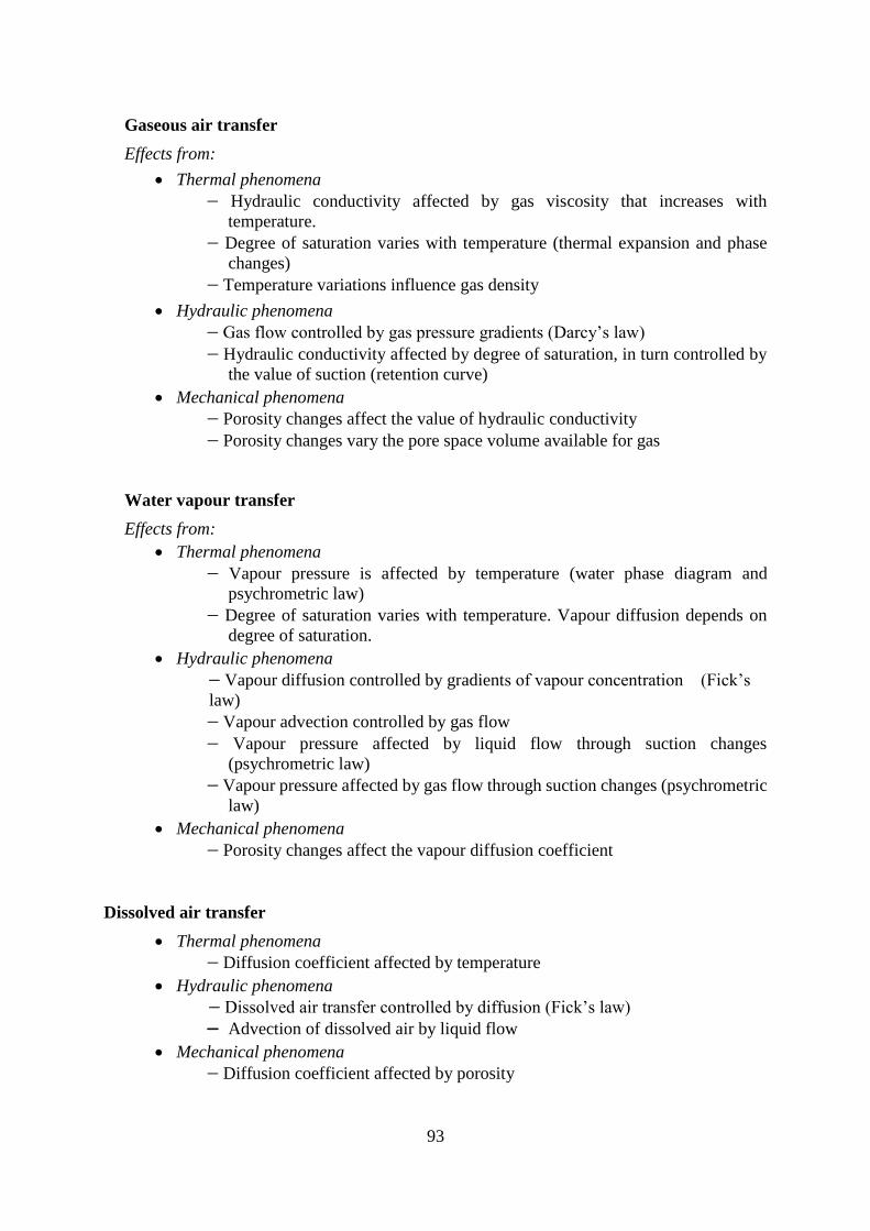
93
Gaseous air transfer
Effects from:
Thermal phenomena
Hydraulic conductivity affected by gas viscosity that increases with
temperature.
Degree of saturation varies with temperature (thermal expansion and phase
changes)
Temperature variations influence gas density
Hydraulic phenomena
Gas flow controlled by gas pressure gradients (Darcy’s law)
Hydraulic conductivity affected by degree of saturation, in turn controlled by
the value of suction (retention curve)
Mechanical phenomena
Porosity changes affect the value of hydraulic conductivity
Porosity changes vary the pore space volume available for gas
Water vapour transfer
Effects from:
Thermal phenomena
Vapour pressure is affected by temperature (water phase diagram and
psychrometric law)
Degree of saturation varies with temperature. Vapour diffusion depends on
degree of saturation.
Hydraulic phenomena
Vapour diffusion controlled by gradients of vapour concentration (Fick’s
law)
Vapour advection controlled by gas flow
Vapour pressure affected by liquid flow through suction changes
(psychrometric law)
Vapour pressure affected by gas flow through suction changes (psychrometric
law)
Mechanical phenomena
Porosity changes affect the vapour diffusion coefficient
Dissolved air transfer
Thermal phenomena
Diffusion coefficient affected by temperature
Hydraulic phenomena
Dissolved air transfer controlled by diffusion (Fick’s law)
Advection of dissolved air by liquid flow
Mechanical phenomena
Diffusion coefficient affected by porosity

94
MECHANICAL PHENOMENA
Stress/strain field
Effects from:
Thermal phenomena
Thermal expansion of materials
Dependence of constitutive laws on temperature
Hydraulic phenomena
Dependence of constitutive laws on suction
Mechanical phenomena
Stress/strain constitutive laws
_________________________________

95
VI. CODE_BRIGHT. CONSTITUTIVE LAWS
This chapter contains the different models available and the corresponding parameters required
by each model. The following constitutive laws are available
HYDRAULIC AND
THERMAL CONSTITUTIVE
MODELS (a)
RETENTION CURVE
INTRINSIC PERMEABILITY
LIQUID PHASE RELATIVE
PERMEABILITY
GAS PHASE RELATIVE
PERMEABILITY
DIFFUSIVE FLUXES OF MASS
DISPERSIVE FLUXES OF
MASS AND ENERGY
CONDUCTIVE FLUX OF HEAT
MECHANICAL CONSTITUTIVE MODELS
ELASTICITY (b)
NONLINEAR ELASTICITY (b)
VISCOPLASTICITY FOR SALINE MATERIALS
(b)
VISCOPLASTICITY FOR SATURATED SOILS
AND ROCKS (b)
VISCOPLASTICITY - GENERAL (b)
DAMAGE-ELASTOPLASTIC MODEL FOR
ARGILLACEOUS ROCKS (c)
THERMOELASTOPLASTIC MODEL FOR SOILS
(d)
BARCELONA EXPANSIVE MODEL FOR SOILS
(e)
CASM’s FAMILY MODELS (f)
PHASE PROPERTIES (a)
SOLID PHASE PROPERTIES
LIQUID PHASE PROPERTIES
GAS PHASE PROPERTIES
EXCAVATION PROCESS (g)
VI.a HYDRAULIC AND THERMAL CONSTITUTIVE LAWS. PHASE PROPERTIES
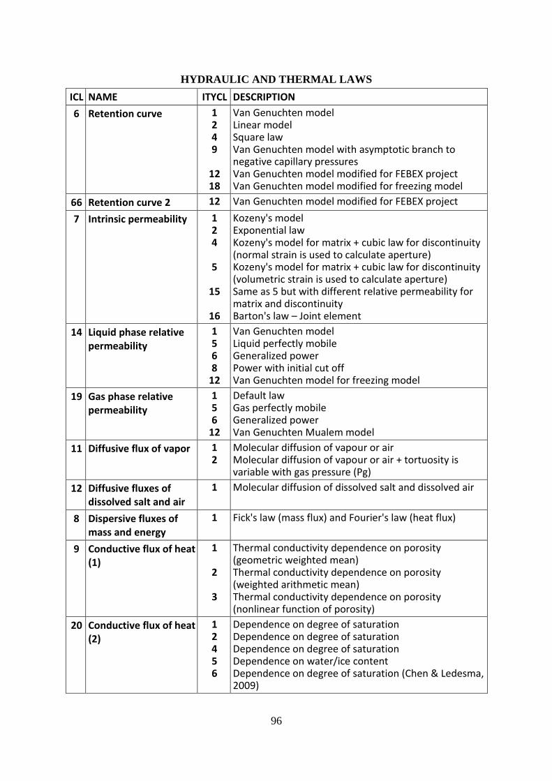
96
HYDRAULIC AND THERMAL LAWS
ICL NAME ITYCL DESCRIPTION
6 Retention curve 1 2 4 9
12 18
Van Genuchten model Linear model Square law Van Genuchten model with asymptotic branch to negative capillary pressures Van Genuchten model modified for FEBEX project Van Genuchten model modified for freezing model
66 Retention curve 2 12 Van Genuchten model modified for FEBEX project
7 Intrinsic permeability 1 2 4
5
15
16
Kozeny's model Exponential law Kozeny's model for matrix + cubic law for discontinuity (normal strain is used to calculate aperture) Kozeny's model for matrix + cubic law for discontinuity (volumetric strain is used to calculate aperture) Same as 5 but with different relative permeability for matrix and discontinuity Barton's law – Joint element
14 Liquid phase relative permeability
1 5 6 8
12
Van Genuchten model Liquid perfectly mobile Generalized power Power with initial cut off Van Genuchten model for freezing model
19 Gas phase relative permeability
1 5 6
12
Default law Gas perfectly mobile Generalized power Van Genuchten Mualem model
11 Diffusive flux of vapor 1 2
Molecular diffusion of vapour or air Molecular diffusion of vapour or air + tortuosity is variable with gas pressure (Pg)
12 Diffusive fluxes of dissolved salt and air
1 Molecular diffusion of dissolved salt and dissolved air
8 Dispersive fluxes of mass and energy
1 Fick's law (mass flux) and Fourier's law (heat flux)
9 Conductive flux of heat (1)
1
2
3
Thermal conductivity dependence on porosity (geometric weighted mean) Thermal conductivity dependence on porosity (weighted arithmetic mean) Thermal conductivity dependence on porosity (nonlinear function of porosity)
20 Conductive flux of heat (2)
1 2 4 5 6
Dependence on degree of saturation Dependence on degree of saturation Dependence on degree of saturation Dependence on water/ice content Dependence on degree of saturation (Chen & Ledesma, 2009)

97
PHASE PROPERTIES
ICL NAME ITYCL DESCRIPTION
10 Solid phase properties 1 2
Solid specific heat, density and expansion coefficient Solid specific heat, density and expansion coeff. (variation of solid phase specific heat)
15 Liquid phase properties: density
1 2 4 5
6
Liquid density (exponential variation) Liquid density (linear variation) Liquid density (CO2)
Liquid density (linear dependency of the thermal expansion coefficient with temperature) Liquid density adjustment for a wide temperature range (-30ºC—300ºC)
16 Liquid phase properties: viscosity
1 Liquid viscosity
17 Gas phase properties: density
1
2
3
4
Dry air density. Law of ideal gases and Henry's law for dry air Usually used to consider a second liquid phase instead of the gas phase Like ITYCL=1 but with user defined values for gas molecular mass and Henry's constant Gas density CO2
18 Gas phase properties: viscosity
1 2 4
Gas viscosity Gas viscosity (exponential law) Gas viscosity CO2

98
RETENTION CURVE
CODES in ROOT_gen.dat
ICL = 6 ITYCL = 1, 2, 4, 9, 12, 18
(See ICL = 66 for ITYCL = 1, 9, 12, 18)
DESCRIPTION Curve capillary pressure versus degree of saturation.
EQUATIONS ITYCL = 1: Van Genuchten model:
1
1
1g ll rl
e o
ls rl o
P PS SS P P
S S P
ITYCL = 2: Linear model: SS S
S S
P P
Pe
l rl
ls rl
g l
o
1
ITYCL = 4: Square law: SS S
S S P P
P
e
l rl
ls rl g l
o
1
1
ITYCL = 9: Van Genuchten model with asymptotic branch that goes to
negative capillary pressures.
1
1
2
1
g ll rl oe g l o
ls rl o
l ls g l
g l
P PS S PS P P a P P
S S P f
bS S P P a
P P a c
where b,c are internal smoothing functions.
ITYCL = 12: FEBEX model:
1
1
1
1
d
g ll rle d
ls rl
g lo d
o d
P PS SS f
S S P
P PP P f
P
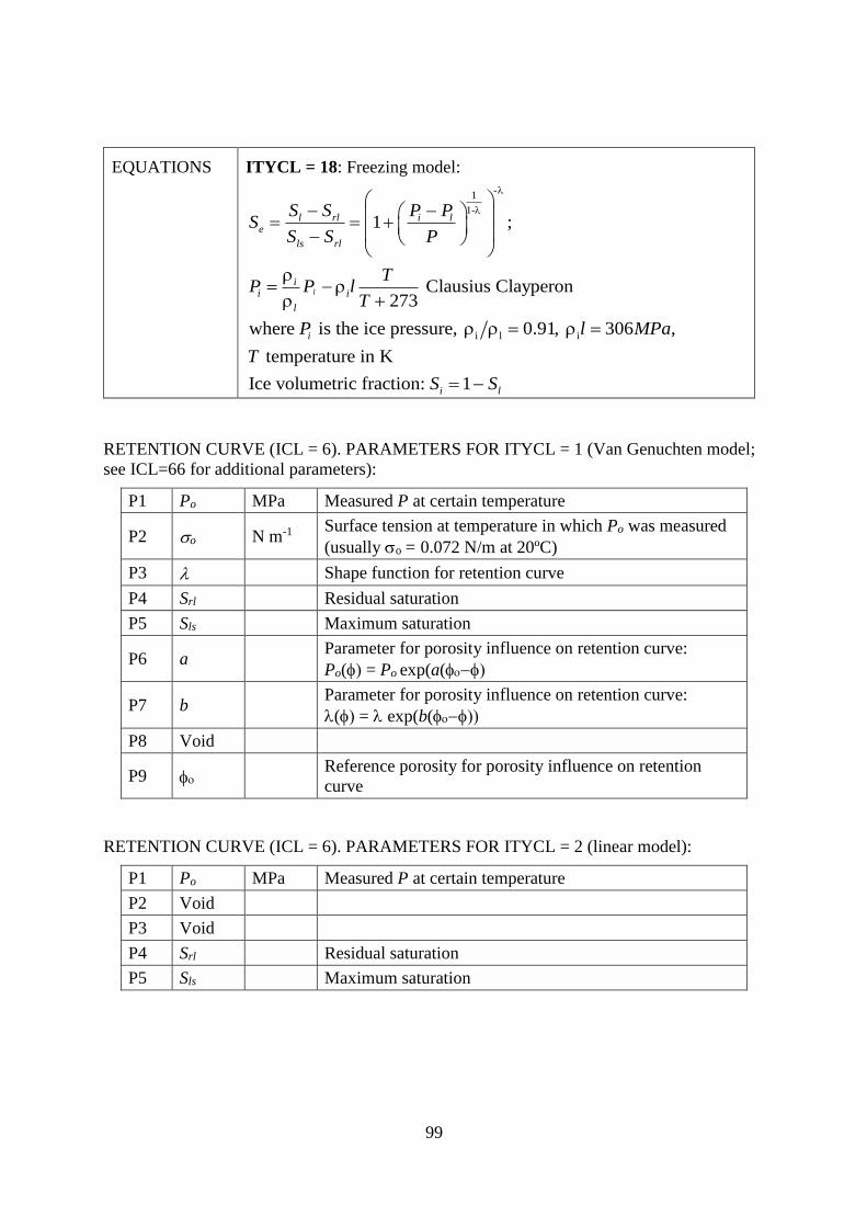
99
RETENTION CURVE (ICL = 6). PARAMETERS FOR ITYCL = 1 (Van Genuchten model;
see ICL=66 for additional parameters):
P1 Po MPa Measured P at certain temperature
P2 o N m-1 Surface tension at temperature in which Po was measured
(usually o = 0.072 N/m at 20ºC)
P3 Shape function for retention curve
P4 Srl Residual saturation
P5 Sls Maximum saturation
P6 a Parameter for porosity influence on retention curve:
Po(= Po exp(a(
P7 b Parameter for porosity influence on retention curve:
(= exp(b(
P8 Void
P9 Reference porosity for porosity influence on retention
curve
RETENTION CURVE (ICL = 6). PARAMETERS FOR ITYCL = 2 (linear model):
P1 Po MPa Measured P at certain temperature
P2 Void
P3 Void
P4 Srl Residual saturation
P5 Sls Maximum saturation
EQUATIONS ITYCL = 18: Freezing model:
-1
1-
i l i
1 ;
Clausius Clayperon 273
where is the ice pressure, 0.91, 306 ,
temperature in K
Ice volumetric fraction: 1
l
l rl i le
ls rl
ii i
l
i
i l
S S P PS
S S P
TP P l
T
P l MPa
T
S S

100
RETENTION CURVE (ICL = 6). PARAMETERS FOR ITYCL = 4 (square law):
P1 Po MPa Measured P at certain temperature
P2 Void
P3 Void
P4 Srl Residual saturation
P5 Sls Maximum saturation
RETENTION CURVE (ICL = 6). PARAMETERS FOR ITYCL = 9 (Van Genuchten model
with asymptotic branch that goes to negative capillary pressures; see ICL=66 for additional
parameters):
P1 Po MPa Measured P at certain temperature
P2 o N m-1 Surface tension at temperature in which Po was measured
(usually o=0.072 N/m at 20ºC)
P3 Shape function for retention curve
P4 Srl Residual saturation
P5 Sls Maximum saturation
P6 f Used for the asymptotic branch
RETENTION CURVE (ICL = 6). PARAMETERS FOR ITYCL = 12 (FEBEX model; see
ICL=66 for additional parameters):
P1 Po MPa Measured P at certain temperature
P2 o N m-1 Surface tension at temperature in which Po was measured
(usually o=0.072 N/m at 20ºC)
P3 Shape function for retention curve
P4 Srl Residual saturation
P5 Sls Maximum saturation
P6 a
Parameter for porosity influence on retention curve:
Po(=Po exp(a(Pd(=Pd exp(a(
See Retention curve 2 (ICL=66) for additional parameters.
P7 b
Parameter for porosity influence on retention curve:
(= exp(b(d (=d exp(b(
See Retention curve 2 (ICL=66) for additional parameters.
P8 Reference porosity for porosity influence on retention
curve
P9 Pd MPa Pressure related with the suction at zero degree of
saturation
P10 d Model parameter

101
RETENTION CURVE (ICL = 6). PARAMETERS FOR ITYCL = 18 (freezing model; see
ICL=66 for additional parameters):
P1 Po MPa Measured P at certain temperature
P2 o N m-1 Surface tension at temperature in which Po was measured
(usually o = 0.072 N/m at 20ºC)
P3 Shape function for retention curve
P4 Srl Residual saturation
P5 Sls Maximum saturation
P6 a Parameter for porosity influence on retention curve:
Po(= Po exp(a(
P7 b Parameter for porosity influence on retention curve:
(= exp(b(
P8 Void
P9 Reference porosity for porosity influence on retention
curve
P10 i_stress
Flag to indicate stress concept for use in the mechanical
model:
i_stress = 0 : Net stress (n = - Pi)
i_stress = -1: Bishop’s stress (b = - Pi + Sr (Pi-Pl))
Srl and Sls are lower and upper bounds of saturation. Effective saturation Se is defined in such a
way that ranges between 0 and 1.

102
RETENTION CURVE 2
RETENTION CURVE (ICL = 66). PARAMETERS FOR ITYCL = 1, 9, 12, 18
P1* 𝐴 𝐶−1
Parameter 𝐴 for temperature influence on capillary
pressure parameter P:
𝑃 = 𝑃0𝜎
𝜎0exp(𝐴(𝑇 − 𝑇0))
P2* 𝑇0 𝐶
Parameter 𝑇0 for temperature influence on capillary
pressure parameter P:
𝑃 = 𝑃0𝜎
𝜎0exp(𝐴(𝑇 − 𝑇0))
* Note that to be able to use the function 𝑃 = 𝑃0𝜎
𝜎0exp(𝐴(𝑇 − 𝑇0)), it is required to input a
value for 𝜎0 (usually 0.072 N/m at 20ºC) in ICL = 6 (retention curve).
RETENTION CURVE (ICL = 66). PARAMETERS FOR ITYCL = 12 (FEBEX model):
P6 ad Parameter for porosity influence on retention curve:
Pd (= Pd exp(ad (
P7 bd Parameter for porosity influence on retention curve:
d (=d exp(bd (
CODES in
ROOT_gen.dat
ICL = 66 ITYCL = 1, 9, 12, 18
DESCRIPTION Curve capillary pressure versus degree of saturation. Additional
parameters for retention curve ICL = 6.
EQUATIONS ITYCL = 1, 9, 12, 18: Temperature influence on capillary pressure
parameter P:
𝑃 = 𝑃0𝜎
𝜎0exp(𝐴(𝑇 − 𝑇0))
ITYCL = 12: FEBEX model:
1
1
1
1
d
g ll rle d
ls rl
g lo d
o d
P PS SS f
S S P
P PP P f
P

103
INTRINSIC PERMEABILITY
CODES in
ROOT_gen.dat ICL = 7 ITYCL = 1, 2, 4, 5, 6, 15, 16
DESCRIPTION Intrinsic permeability
EQUATIONS ITYCL = 1: For a continuum medium (Kozeny’s model): 23
2 3
(1 ): reference porosity
(1 )
: intrinsic permeability for matrix
oo o
o
o o
k k
k
which is used in Darcy’s law: qk
g
kP
r
where viscosity, density and relative permeability are defined in other laws.
ITYCL = 2: Exponential law: expo o
b k k
ITYCL = 4, 5: Intrinsic permeability depending on an embedded aperture: 3
12matrix
b
a k k ob b b ( ) for o ob a a
where matrixk : reference intrinsic permeability of the rock matrix or
porous material (without fractures).
a: spacing of the fracture.
b: variable aperture as a function of normal or volumetric strains.
b0: minimum aperture.
Using this option, the capillary pressure P of the retention curve (ICL=6)
varies as:
3
0
3oP Pk
k
where Po is the capillary pressure for a reference permeability ko, which
can be the initial permeability.
ITYCL = 6: Postfailure model: ok k (pre-failure)
3exp 1 exp v B
o c
B
k k k (post-failure)
ITYCL = 15: This model is similar to option ITYCL=5 except that:
𝐤𝑘𝑟𝑔 = 𝐤𝑚𝑎𝑡𝑟𝑖𝑥𝑘𝑟𝑔𝑚𝑎𝑡𝑟𝑖𝑥 + 𝐤𝑓𝑟𝑎𝑐𝑡𝑢𝑟𝑒𝑘𝑟𝑔
𝑑𝑖𝑠𝑐𝑜𝑛𝑡𝑖𝑛𝑢𝑖𝑡𝑦
where relative permeability is split into two functions depending if the
intrinsic permeability corresponds to the matrix or the discontinuity:
𝑘𝑟𝑔𝑚𝑎𝑡𝑟𝑖𝑥 is calculated normally, and 𝑘𝑟𝑔
𝑑𝑖𝑠𝑐𝑜𝑛𝑡𝑖𝑛𝑢𝑖𝑡𝑦= 𝑆𝑔 = (1 − 𝑆𝑙)

104
ITYCL = 16: Zero thickness element
Barton’s law: Longitudinal intrinsic permeability 2
2 2
2.5
1
12 12l
e ak
JRC
: Opening of the joint: Joint Roughness Coefficient
aJRC
Transversal intrinsic permeability tk is considered to be equal to the
continuum media.
For the retention curve (ICL=6), air entry value depends on joint aperture,
as: 0
00
l
l
kP P
k
INTRINSIC PERMEABILITY (ICL = 7). PARAMETERS FOR ITYCL = 1
P1 (k11)o m2 Intrinsic permeability, 1st principal direction.
P2 (k22)o m2 Intrinsic permeability, 2nd principal direction.
P3 (k33)o m2 Intrinsic permeability, 3rd principal direction.
P4 o Reference porosity for read intrinsic permeability.
If o=0, permeability will be constant.
P5 min Minimum porosity (porosity will not be lower than this value).
INTRINSIC PERMEABILITY (ICL = 7). PARAMETERS FOR ITYCL = 2
P1-P5 The same as in ITYCL=1
P6 b - Parameter.
INTRINSIC PERMEABILITY (ICL = 7). PARAMETERS FOR ITYCL = 4, 5, 15
P1-P5 The same as in ITYCL=1
P7 bo m Minimum aperture to calculate a variable aperture as: ob b b
P8 a m Spacing of the fractures:
3
12matrix
bk k
a
Permeability of the matrix is obtained as usual in porous media.
P9 o -
Reference strain to calculate aperture variations: ( ) for o ob a a
If this value is negative, the initial aperture is larger than the
minimum aperture (discontinuity is open).
If this value is zero or positive, the discontinuity cannot close.
P10 bmax m Maximum aperture. Upper bound of aperture.

105
To use ITYCL=4, 5, 15, the reference porosity (P4) needs to be greater than zero.
For ITYCL=4, the normal strain to the discontinuity is used.
For ITYCL=5, 15 the volumetric strain is used.
INTRINSIC PERMEABILITY (ICL=7). PARAMETERS FOR ITYCL=6
P1-P5 The same as in ITYCL = 1
P6 γ MPa-1 Dilatability
P7 B - Maximum volumetric strain
P9 Kc - Permeability at zero minor principal stress
INTRINSIC PERMEABILITY (ICL=7). PARAMETERS FOR ITYCL=16
P1 (k11)o m2
Longitudinal intrinsic permeability, 1st principal direction.
If (k11)0 = 1, the intrinsic permeability, lk , is calculated with Barton’s
law. Permeability and air entry value depends on joint aperture.
P2 (k22)o m2 Transversal intrinsic permeability, tk , 2nd principal direction.
P4-P5 The same as in ITYCL = 1
P6 JRC - Joint Roughness Coefficient.
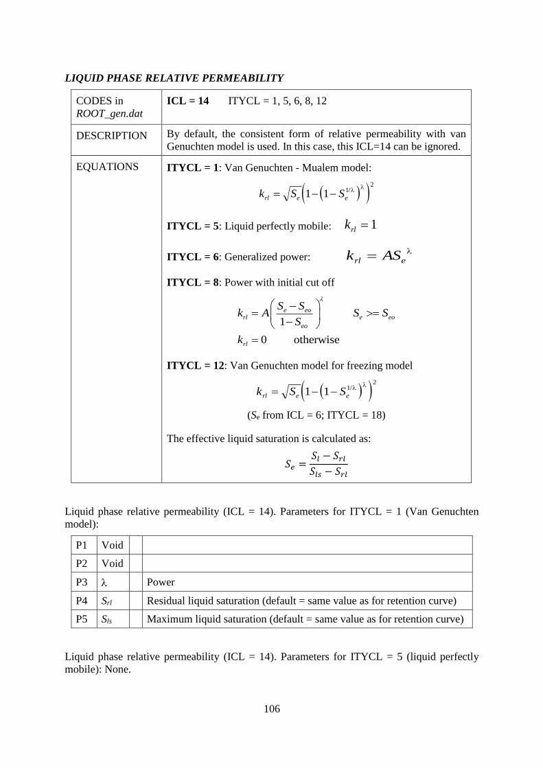
106
LIQUID PHASE RELATIVE PERMEABILITY
CODES in
ROOT_gen.dat
ICL = 14 ITYCL = 1, 5, 6, 8, 12
DESCRIPTION By default, the consistent form of relative permeability with van
Genuchten model is used. In this case, this ICL=14 can be ignored.
EQUATIONS ITYCL = 1: Van Genuchten - Mualem model:
k S Srl e e 1 1 12
/
ITYCL = 5: Liquid perfectly mobile: krl 1
ITYCL = 6: Generalized power: k ASrl e
ITYCL = 8: Power with initial cut off
1
0 otherwise
e eorl e eo
eo
rl
S Sk A S S
S
k
ITYCL = 12: Van Genuchten model for freezing model
k S Srl e e 1 1 12
/
(Se from ICL = 6; ITYCL = 18)
The effective liquid saturation is calculated as:
𝑆𝑒 =𝑆𝑙 − 𝑆𝑟𝑙𝑆𝑙𝑠 − 𝑆𝑟𝑙
Liquid phase relative permeability (ICL = 14). Parameters for ITYCL = 1 (Van Genuchten
model):
P1 Void
P2 Void
P3 Power
P4 Srl Residual liquid saturation (default = same value as for retention curve)
P5 Sls Maximum liquid saturation (default = same value as for retention curve)
Liquid phase relative permeability (ICL = 14). Parameters for ITYCL = 5 (liquid perfectly
mobile): None.

107
Liquid phase relative permeability (ICL = 14). Parameters for ITYCL=6 (generalized power):
P1 Void
P2 A Constant
P3 Power (typically 3)
P4 Srl Residual liquid saturation (default = same value as for retention curve)
P5 Sls Maximum liquid saturation (default = same value as for retention curve)
Liquid phase relative permeability (ICL = 14). Parameters for ITYCL = 8 (power with initial
cut off):
P1 Seo Parameter
P2 A Constant
P3 Power
P4 Srl Residual liquid saturation (default = same value as for retention curve)
P5 Sls Maximum liquid saturation (default = same value as for retention curve)
Liquid phase relative permeability (ICL = 14). Parameters for ITYCL = 12 (Van Genuchten
model for freezing model):
P1 Void
P2 Void
P3 Power
P4 Srl Residual liquid saturation (default = same value as for retention curve)
P5 Sls Maximum liquid saturation (default = same value as for retention curve)
Srl and Sls are lower and upper bounds of liquid saturation. Effective liquid saturation Se is
defined in such a way that ranges between 0 and 1. In principle, the same values Srl and Sls
should be defined for liquid and gas relative permeability and for retention curve. However,
different values can be used to define a maximum saturation of liquid with possibility of
remnant gas flow or vice-versa.

108
GAS PHASE RELATIVE PERMEABILITY
CODES in
ROOT_gen.dat
ICL = 19 ITYCL = 1, 5, 6, 12
DESCRIPTION Relative permeability of the gas phase
EQUATIONS ITYCL = 1: Default law: k krg rl 1
ITYCL = 5: Gas perfectly mobile: krg 1
ITYCL = 6: Generalized power: k ASrg eg
The effective gas saturation is calculated as:
𝑆𝑒𝑔 =𝑆𝑔 − 𝑆𝑟𝑔
𝑆𝑔𝑠 − 𝑆𝑟𝑔
ITYCL = 12: Van Genuchten-Mualem
𝑘𝑟𝑔 = (1 − 𝑆𝑒𝑙)𝛾 (1 − 𝑆𝑒𝑙
1
𝜆 )
2𝜆
The effective liquid saturation can be calculated as:
𝑆𝑒𝑙 = 1 − 𝑆𝑒𝑔 = 1 −𝑆𝑔 − 𝑆𝑟𝑔
𝑆𝑔𝑠 − 𝑆𝑟𝑔
GAS PHASE RELATIVE PERMEABILITY (ICL = 19). PARAMETERS FOR ITYCL = 1
(default law):
P1-P3 Void
P4 Srg - Residual gas saturation (default = 1-Sls in retention curve)
P5 Sgs - Maximum gas saturation (default = 1-Srl in retention curve)
GAS PHASE RELATIVE PERMEABILITY (ICL = 19). PARAMETERS FOR ITYCL = 5
(gas perfectly mobile): None
GAS PHASE RELATIVE PERMEABILITY (ICL = 19). PARAMETERS FOR ITYCL = 6
(generalized power):
P1 Void
P2 A Constant
P3 Power
P4 – P5 The same as in ITYCL = 1
GAS PHASE RELATIVE PERMEABILITY (ICL = 19). PARAMETERS FOR ITYCL = 12:
P1 Void
P2 Power
P3 – P5 The same as in ITYCL = 6

109
DIFFUSIVE FLUXES OF VAPOUR
CODES in
ROOT_gen.dat
ICL = 11 ITYCL = 1, 2
DESCRIPTION Diffusion coefficients
EQUATIONS Fick's law for molecular diffusion is written as:
i i iS D i I
where is porosity, is density, S is degree of saturation, is
mass fraction and Di is the diffusion coefficient of species i in
phase in m2/s.
The non-advective flux of a species in a phase is composed by
molecular diffusion and mechanical dispersion (dispersion is
defined in another set of parameters).
ITYCL = 1: Molecular diffusion of vapour or air in the gas phase:
273.15n
i
g
TD D
P
where Pg is the gas pressure in Pa, and D and n are parameters.
Tortuosity coefficient is defined as a constant value in this case:
0constant =
ITYCL = 2: Molecular diffusion of vapour or air in the gas
phase:
273.15n
i
g
TD D
P
where Pg is the gas pressure in Pa, and D and n are parameters.
Tortuosity coefficient is defined in this case as:
0
m
gS
where 0 and m are parameters.
DIFFUSIVE FLUXES OF VAPOUR (ICL = 11). PARAMETERS FOR ITYCL = 1:
P1 D m2 s-1 K-n Pa Default value = 5.910-6
P2 n Default value = 2.3
P3 0 Coefficient of tortuosity; default = 1.0
DIFFUSIVE FLUXES OF VAPOUR (ICL = 11). PARAMETERS FOR ITYCL = 2:
P1 – P3 The same as in ITYCL = 1
P4 m Power for tortuosity function of saturation

110
DIFFUSIVE FLUXES OF DISSOLVED SALT AND AIR
CODES in
ROOT_gen.dat
ICL = 12 ITYCL = 1
DESCRIPTION Diffusion coefficients
EQUATIONS Fick's law for molecular diffussion is written as:
i i iS D i I
where is porosity, is density, S is degree of saturation, is
mass fraction and Dmi is the diffusion coefficient of species i in
phase in m2/s.
ITYCL = 1: Molecular diffusion of dissolved salt and/or
dissolved air in the liquid phase:
exp
273.15
i QD D
R T
where D and Q are parameters and is the coefficient of
tortuosity.
DIFFUSIVE FLUXES OF DISSOLVED SALT AND AIR (ICL = 12). PARAMETERS FOR
ITYCL = 1:
P1 D m2 s-1 Default value = 1.110-4
P2 Q J mol-1 Default value = 24530
P3 Coefficient of tortuosity; default=1.0
P4 – P10 Void
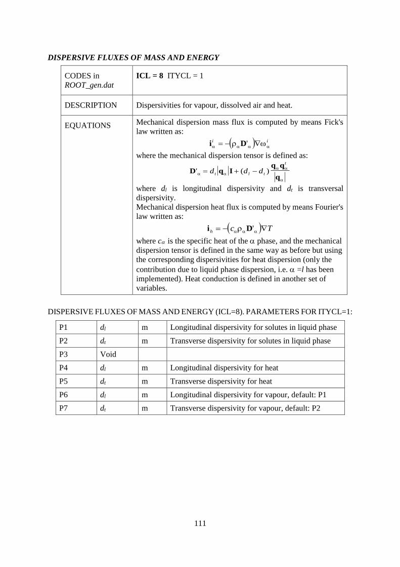
111
DISPERSIVE FLUXES OF MASS AND ENERGY
CODES in
ROOT_gen.dat
ICL = 8 ITYCL = 1
DESCRIPTION Dispersivities for vapour, dissolved air and heat.
EQUATIONS Mechanical dispersion mass flux is computed by means Fick's
law written as:
i D i i '
where the mechanical dispersion tensor is defined as:
D q Iq q
q' ( )
d d dt l t
t
where dl is longitudinal dispersivity and dt is transversal
dispersivity.
Mechanical dispersion heat flux is computed by means Fourier's
law written as:
i Dh c T '
where cis the specific heat of the phase, and the mechanical
dispersion tensor is defined in the same way as before but using
the corresponding dispersivities for heat dispersion (only the
contribution due to liquid phase dispersion, i.e. =l has been
implemented). Heat conduction is defined in another set of
variables.
DISPERSIVE FLUXES OF MASS AND ENERGY (ICL=8). PARAMETERS FOR ITYCL=1:
P1 dl m Longitudinal dispersivity for solutes in liquid phase
P2 dt m Transverse dispersivity for solutes in liquid phase
P3 Void
P4 dl m Longitudinal dispersivity for heat
P5 dt m Transverse dispersivity for heat
P6 dl m Longitudinal dispersivity for vapour, default: P1
P7 dt m Transverse dispersivity for vapour, default: P2

112
CONDUCTIVE FLUX OF HEAT (1)
CODES in
ROOT_gen.dat
ICL = 9 ITYCL = 1, 2, 3
DESCRIPTION Dependence on porosity and temperature.
EQUATIONS Thermal conductivity is used in Fourier's law to compute conductive
heat flux, i.e.:
ic T
There are two possibilities to solve conductive flux of heat through this
law:
a) Giving directly dry and sat. These values can be measured in the
laboratory. They will be used in law ICL=20.
b) Giving the conductivity of the phases of the soil, i.e. (solid)o, liquid,
gas and a1, a2, a3. In this case, dry and sat are calculated according
to the laws given below.
ITYCL = 1: Thermal conductivity dependence on porosity. Geometric
weighted mean.
dry solid gas sat solid liq ( ) ( )1 1
solid solid o a T a T a T ( ) 1 2
2
3
3
ITYCL = 2: Thermal conductivity dependence on porosity. Weighted
arithmetic mean.
dry
n
solid
n
gas sat
n
solid
n
liq ( ) ( )1 1
ITYCL = 3: Thermal conductivity dependence on porosity. Nonlinear
function of porosity.
n
dry solid dryo solid
o
n
sat solid sato solid
o

113
CONDUCTIVE FLUX OF HEAT 1 (ICL = 9). PARAMETERS FOR ITYCL = 1 (geometric
weighted mean):
P1 dry W m-1 K-1 Thermal conductivity of the dry porous medium
P2 sat W m-1 K-1 Thermal conductivity of the water saturated porous
medium
P3 (solid)o W m-1 K-1 Solid phase thermal conductivity (ignored if dry, sat>0)
P4 gas W m-1 K-1 Gas phase thermal conductivity (ignored if dry, sat>0)
P5 liq W m-1 K-1 Liquid phase thermal conductivity (ignored if dry, sat>0)
P6 a1 Ignored if dry, sat 0
P7 a2 Ignored if dry, sat 0
P8 a3 Ignored if dry, sat 0
CONDUCTIVE FLUX OF HEAT 1 (ICL = 9). PARAMETERS FOR ITYCL = 2 (weighted
arithmetic mean):
P1 – P8 The same as in ITYCL = 1
P9 Void
P10 n Power of porosity function (default value = 1, so linear
dependence with porosity)
CONDUCTIVE FLUX OF HEAT 1 (ICL = 9). PARAMETERS FOR ITYCL = 3 (nonlinear
function of porosity):
P1 – P2 Void
P3 (solid)o W m-1 K-1 Solid phase thermal conductivity
P4 (dry)o W m-1 K-1 Dry thermal conductivity for reference porosity
P5 (sat) o W m-1 K-1 Saturated thermal conductivity for reference porosity
P6 – P8 Void
P9 o Reference porosity
P10 n Power of porosity
Heat dispersion is defined in the constitutive law ICL = 8, ITYCL = 1 (Dispersive fluxes of
mass and energy).

114
CONDUCTIVE FLUX OF HEAT (2)
CODES in
ROOT_gen.dat ICL = 20 ITYCL = 1, 2, 4, 5, 6, 7
DESCRIPTION Dependence on water content.
EQUATIONS Thermal conductivity is used in Fourier's law to compute conductive heat flux,
i.e.:
ic T
Dependence of thermal conductivity on degree of saturation can be considered
in the following ways:
ITYCL = 1: Linear with the square root of saturation
sat l dry lS S1
ITYCL = 2: Geometric mean:
sat
S
dry
Sl l1
ITYCL = 4: Linear with saturation: 1dry l sat lS S
ITYCL = 5: Geometric mean for frozen soil
Dependence on water/ice content. Activating this option permits to have
different values for thermal conductivity depending if the soil is frozen or
unfrozen.
1 llSS
unfrozen frozen
frozen = dry and unfrozen = sat, are introduced in ICL = 9, ITYCL = 1.
The thermal conductivity of phases can be introduced to determine the
thermal conductivity of the frozen and unfrozen soil. In such case the solid
and liquid water are input as usual, and the ice thermal conductivity should
be input in the same place as the gas thermal conductivity
ITYCL = 6: Dependence of thermal conductivity on degree of saturation
(Chen & Ledesma, 2009):
2 2sin cos2 2
l lsat dry
S S
ITYCL = 7: S-shaped function
λ =A1 − A2
1 + 𝑒[(𝑆𝑟−𝑆𝑟∗)
𝑏⁄ ]+ A2
Where A1 represents the value of for 𝑆𝑟 = 1, A2 the value of for 𝑆𝑟 = 0,
𝑆𝑟∗ the degree of saturation for which thermal conductivity is the average of
the two extreme values and b is a parameter. In some cases, A1 and A2 are
equivalent to sat and dry, respectively. A1 and A2 are introduced as sat and
dry in ICL = 9, ITYCL = 1: Conductive flux of heat (1).
Parameters are not necessary for ICL = 20 and ITYCL = 1, 2, 4, 5, 6.
dry and sat are introduced in ICL = 9: Conductive flux of heat (1).

115
CONDUCTIVE FLUX OF HEAT 2 (ICL = 20). PARAMETERS FOR ITYCL = 7 (S-shaped
function):
P1 𝑏 - Parameter (since 𝐴1 > 𝐴2 , this parameter is negative for the
equation written above, so it must be input as a negative value).
P2 𝑆𝑟∗ - Degree of saturation corresponding to a value of thermal
conductivity that is the average between the extreme values
CONDUCTIVE FLUX WITH ANISOTROPY:
CONDUCTIVE FLUX OF HEAT 1 (ICL = 9): leave all parameters void.
CONDUCTIVE FLUX OF HEAT 2 (ICL = 20): ITYCL = 1:
P6 λ11 W/(mK) Thermal conductivity in 1st principal direction
P7 λ22 W/(mK) Thermal conductivity in 2nd principal direction
P8 λ33 W/(mK) Thermal conductivity in 3rd principal direction
Note this option does not allow using porosity, degree of saturation or temperature
dependencies.

116
PHASE PROPERTIES
SOLID PHASE PROPERTIES
CODES in
ROOT_gen.dat
ICL = 10 ITYCL = 1, 2
DESCRIPTION Solid specific heat, density and expansion coefficient
SOLID PHASE PROPERTIES (ICL = 10). PARAMETERS FOR ITYCL = 1:
P1 Cs J kg-1 K-1 Solid phase specific heat (default: 1000) (**)
P2 s kg m-3 Solid phase density (default: 2700)
P3 s C-1
Linear thermal expansion coefficient for grains (not
volumetric) (positive value; default = 1E-5). This does not
produce thermal expansion of the medium. (*)
P4 To C Reference temperature for thermal expansion (default: 40)
P5 – P6 void
P7 1/Ks MPa-1 Compressibility of solid phase against mean stress changes
(positive value; default = 3E-5)
P8 po MPa Reference pressure for solid compressibility (default: 0.1
MPa)
SOLID PHASE PROPERTIES (ICL = 10). PARAMETERS FOR ITYCL = 2:
P1 cs J kg-1 K-1 Solid phase specific heat for T = 0 (default: 1000)
P2 – P5 The same as in ITYCL = 1
P6 dcs/dt Variation of solid phase specific heat
P7 – P8 The same as in ITYCL = 1
(*) Thermal expansion coefficient for grains should be equal to the bulk value if thermal
expansion of the porous medium does not produce porosity variations.
(**) Specific heat for water and air are internal values.

117
LIQUID PHASE PROPERTIES. LIQUID DENSITY.
CODES in
ROOT_gen.dat
ICL = 15 ITYCL = 1, 2, 3, 4, 5, 6
DESCRIPTION Liquid density
EQUATIONS ITYCL = 1: Exponential variation (default):
0 exp( ( ) )h
l l l lo lP P T
ITYCL = 2: Linear variation:
0(1 ( ) )h
l l l lo lP P T
ITYCL = 4: CO2
2
0 0exp 1h CO
l l l l l lP P T
2
2 4 2 7 3 6 3
1
37.51 9.585 10 8.740 10 5.044 10 10 m /mol
l
CO
V
M
V T T T
(Garcia, 2003)
ITYCL = 5: Linear dependency of the thermal expansion
coefficient with temperature:
h
l l l lo lP P A T T 0 exp( ( ) )
A T T 6 53.5 10 7.49 10
ITYCL = 6: Liquid density adjustment for a wide temperature
range (-30ºC—300ºC):
h
l l l lo lP P A T 0(1 ( ) )
TT T TA 2( 288.9414)( 3.9863) /(508929.2( 68.12963))
(McCutcheon et al., 1993).
l 3
0 1000 kg/m (note that in this case l0 is not user defined as
it corresponds to the maximum density of water at 4ºC).
Note: the thermal expansion coefficient would be expressed by:
l
l
TT
1

118
LIQUID PHASE DENSITY (ICL = 15). PARAMETERS FOR ITYCL = 1, 2:
P1 lo kg m-3 Reference density (default* = 1002.6 kg m-3)
P2 MPa-1 Compressibility (default* = 4.510-4)
P3 C-1 Volumetric thermal expansion coefficient for water
(default* = -3.410-4)
P4 Solute variation (default* = 0.6923)
P5 Plo MPa Reference pressure (default* = 0.1)
LIQUID PHASE DENSITY (ICL = 15). PARAMETERS FOR ITYCL = 4 (CO2):
P1 – P3 The same as in ITYCL = 1
P4 void
P5 The same as in ITYCL = 1
P6 MCO2 kg mol-1 Molecular mass of CO2 (0.044 kg mol-1)
LIQUID PHASE DENSITY (ICL = 15). PARAMETERS FOR ITYCL = 5:
P1 – P2 The same as in ITYCL = 1
P3 void
P4 – P5 The same as in ITYCL = 1
LIQUID PHASE DENSITY (ICL = 15). PARAMETERS FOR ITYCL = 6:
P1 void
P2 The same as in ITYCL = 1
P3 void
P4 – P5 The same as in ITYCL = 1
* Note that, in the case of parameters with default values, when setting them to zero –or to a
value lower than 10-25– automatically takes the default value. Hence, if the user actually wants
to set a parameter to zero, a low value but greater than 10-25 should be input.

119
EQUIVALENT DENSITY AND SPECIFIC HEAT FOR A TM PROBLEM:
Temperature distribution and evolution in a porous medium is strongly affected by the specific
heat of the water. When a porous material is modelled under TM conditions, equivalent
parameters should be used in order to get realistic and comparable results with THM. Hence, it
is explained here how to calculate those equivalent parameters.
Heat capacity of porous medium for a THM problem in a saturated porous medium:
𝜌𝑠𝑐𝑠(1 − 𝜙) + 𝜌𝑙𝑐𝑙𝜙
Where phase densities, phase specific heats and porosity can be used with their realistic value.
Heat capacity for a TM problem in an equivalent medium: (𝜌𝑠)𝑒𝑞(𝑐𝑠)𝑒𝑞(1 − 𝜙)
To obtain the same stresses induced by weight, an equivalent density for a TM problem in a
saturated porous medium can be calculated as:
(𝜌𝑠)𝑒𝑞 = 𝜌𝑠(1 − 𝜙) + 𝜌𝑙𝜙
(1 − 𝜙)
And to obtain the same temperature, an equivalent specific heat for a TM problem in a
saturated porous medium can be calculated as:
(𝑐𝑠)𝑒𝑞 = 𝜌𝑠𝑐𝑠(1 − 𝜙) + 𝜌𝑙𝑐𝑙𝜙
(𝜌𝑠)𝑒𝑞(1 − 𝜙)

120
LIQUID PHASE PROPERTIES. LIQUID VISCOSITY.
CODES in
ROOT_gen.dat
ICL = 16 ITYCL = 1
DESCRIPTION Liquid viscosity
EQUATIONS ITYCL = 1: l A
B
T
exp
.27315
LIQUID PHASE VISCOSITY (ICL=16). PARAMETERS FOR ITYCL=1:
P1 A MPa s Pre-exponential parameter (default* = 2.110-12)
P2 B K Exponential parameter; default* = 1808.5 (only used
if A = B = 0, but not used if A > 0 and B = 0)
Remark: liquid and gas density and viscosity are not material dependents. For this reason,
values should be prescribed only once. If these are multiplied defined, the code will use the
values it reads first.
* Note that, in the case of parameters with default values, when setting them to zero –or to a
value lower than 10-25– automatically takes the default value. Hence, if the user actually wants
to set a parameter to zero, a low value but greater than 10-25 should be input.

121
GAS PHASE PROPERTIES. GAS DENSITY.
CODES in
ROOT_gen.dat
ICL = 17 ITYCL = 1, 2, 3, 4
DESCRIPTION Gas density.
EQUATIONS ITYCL = 1: law of ideal gases and Henry's law for dry air (as
ITYCL = 3 with Ma = 0.02895 and H = 10000 MPa)
ITYCL = 2: a a
g g g gooP P T exp( ( ) )
Usually used to consider a second liquid phase instead of the
gas phase (in that case do not consider vapour in gas phase)
ITYCL = 3: law of ideal gases and Henry’s law for any dry gas
species (as ITYCL=1, but with user defined values for gas
molecular mass and Henry’s constant:
dgs dgsdgs
l
w
P M
H M
where Pdgs is dry gas species pressure (air pressure in the
formulation), Mw is molecular mass of water and Mdgs is
molecular mass of dry gas species.
ITYCL = 4: law for CO2 with the values adjusted by Spycher
et al., 2003.
2
2
CO
CO
M
5 3
6 0.5 2
2
1 2
1
3
2
2
2.78 10 m /mol
m PaK /mol
7.54 0.0041
0
8.314 J/m
3
olK
b
a
RT RTb a abv v b v
P P P T
a a
P T
R
T
a a
GAS PHASE PROPERTIES (ICL = 17). PARAMETERS FOR ITYCL = 2:
P1 (ga)o kg m-3 Reference density for T = 0 C
P2 MPa-1 Compressibility (default = 0.0)
P3 C-1 Volumetric thermal expansion coefficient for water (default = 0.0)
P4 Void
P5 Pgo MPa Reference pressure (default = 0.0)

122
GAS PHASE PROPERTIES (ICL = 17). PARAMETERS FOR ITYCL = 3 (gases law with
modified molecular mass and Henry’s constant):
P1 M kg mol-1 Molecular mass
P2 H MPa Henry’s constant
GAS PHASE PROPERTIES (ICL = 17). PARAMETERS FOR ITYCL = 4 (law for CO2 with
the values adjusted by Spycher et al., 2003):
P1 MCO2 kg mol-1 Molecular mass of CO2 (0.044 kg mol-1)
P2 H MPa Henry’s constant
P8
Alternative CO2 density function at
T=320 K adjusted from Span and Wagner
(1996) tables. To use it write: -777

123
GAS PHASE PROPERTIES. GAS VISCOSITY.
CODES in
ROOT_gen.dat
ICL = 18 ITYCL = 1, 2, 4
DESCRIPTION Gas viscosity
EQUATIONS ITYCL = 1:
ty)permeabili intrinsic :(
1
1
2731
273
k
DkCb
P
b
T
B
TA
k
g
kg
ITYCL = 2:
T
BAg
15.273exp
ITYCL = 4: Viscosity function for CO2 (Altunin and
Sakhabetdinov, 1972)
4
1
1
0
0 expi j
j
R
i
Rij
gT
a
2
5.0
0
66920556.46346068.162246461.27
RR
RTT
T
c
RT
TT , 304cT K
c
CO
R
2 , 468c kg/m3
248566120.010 a 004894942.011 a
373300660.020 a 22753488.121 a
363854523.030 a 774229021.031 a
0639070755.040 a 142507049.041 a

124
GAS PHASE VISCOSITY (ICL = 18). PARAMETERS FOR ITYCL = 1:
P1 A MPa s default* = 1.48 10-12
P2 B C default* = 119.4 (only used if A = B = 0,
but not used if A > 0 and B = 0)
P3 C default* = 0.14
P4 D default* = 1.2 1015
GAS PHASE VISCOSITY (ICL = 18). PARAMETERS FOR ITYCL = 2:
P1 A MPa s Pre-exponential parameter
P2 B C Exponential parameter (only used if A = B = 0,
but not used if A > 0 and B = 0)
GAS PHASE VISCOSITY (ICL = 18). PARAMETERS FOR ITYCL = 4: Not necessary
Gas phase properties can be used to consider a second liquid in the case of a two immiscible
phase flow problem in a porous medium. In this case, water vapour and air dissolved must not
be considered, hence, VAPOUR NOT PERMITTED and DISSOLVED AIR NOT
PERMITTED should be used to avoid the species to be mixed.
* Note that, in the case of parameters with default values, when setting them to zero –or to a
value lower than 10-25– automatically takes the default value. Hence, if the user actually wants
to set a parameter to zero, a low value but greater than 10-25 should be input.

125
CODE_BRIGHT. CONSTITUTIVE LAWS
This chapter contains the different models available and the corresponding parameters required
by each model. The following constitutive laws are available:
HYDRAULIC AND THERMAL
CONSTITUTIVE MODELS (a)
RETENTION CURVE
INTRINSIC PERMEABILITY
LIQUID PHASE RELATIVE
PERMEABILITY
GAS PHASE RELATIVE
PERMEABILITY
DIFFUSIVE FLUXES OF MASS
DISPERSIVE FLUXES OF MASS
AND ENERGY
CONDUCTIVE FLUX OF HEAT
MECHANICAL CONSTITUTIVE MODELS
ELASTICITY (b)
NONLINEAR ELASTICITY (b)
VISCOPLASTICITY FOR SALINE MATERIALS (b)
VISCOPLASTICITY FOR SATURATED SOILS AND
ROCKS (b)
VISCOPLASTICITY - GENERAL (b)
DAMAGE-ELASTOPLASTIC MODEL FOR
ARGILLACEOUS ROCKS (c)
THERMO-ELASTOPLASTIC MODEL FOR SOILS (d)
BARCELONA EXPANSIVE MODEL (e)
CASM’s FAMILY MODELS (f)
PHASE PROPERTIES (a)
SOLID PHASE PROPERTIES
LIQUID PHASE PROPERTIES
GAS PHASE PROPERTIES
EXCAVATION PROCESS (g)
VI.b. ELASTIC AND VISCO-PLASTIC MODELS
ICL NAME ITYCL DESCRIPTION
1 Linear Elasticity
1
2
5
6
16
Linear elasticity model
Bi-linear elasticity model
Tri-linear elasticity model
Anisotropic elastic model
Elasticity – Zero thickness element
5 1 Linear expansion coefficients induced by temperature and suction changes
4 Nonlinear Elasticity
1
2
5
Volumetric strain is calculated in a reversible way
Nonlinear elasticity model with micro-macro interaction
Volumetric strain is calculated in a reversible way with two independent coupling terms
2 Viscoelasticity - creep 1 Parameters for linear viscous deformation model
3 Viscoplasticity - creep 1 Creep of porous salt aggregates (nonlinear dependences on stresses)
33 Viscoplasticity for saturated soils and rocks (VPSSR)
1,2
3
4,5
9
11
12
15
20
21
Yield function and flow rule
Cam-Clay
Drucker-Prager –based on Mohr-Coulomb parameters
For rock salt with dilatancy
Mohr-Coulomb model with dilatancy
Mohr-Coulomb model with dilatancy and strain-softening
Mohr-Coulomb model with anisotropic behaviour
Hoek-Brown model with dilatancy
Hoek-Brown model with dilatancy and strain-softening
34
Viscoplasticity for unsaturated soils and rocks (VPUSR)
1
16
Viscoplasticity (general model based on Desai and Perzyna theory)
Viscoplasticity – Zero thickness element
35 1
16
Parameters for yield function and plastic potential
Viscoplasticity – Zero thickness element
36
1
2,3
16
Parameters for LC curve
Parameters for LC curve for rockfill materials
Viscoplasticity – Zero thickness element

126
LINEAR ELASTICITY 1 (Mechanical data 1)
CODES in
ROOT_gen.dat
ICL = 1 ITYCL = 1, 2, 5, 6, 16
DESCRIPTION Elastic parameters (linear elasticity model). Linear elasticity with
parameters E and . Young modulus can be variable.
EQUATIONS ITYCL = 1: Linear elasticity model
This is the standard linear elasticity with Young’s Modulus and
Poisson’s ratio.
It is also possible to consider the variation of Young’s Modulus with
porosity, according to:
min( )o o
dEE E E
d
ITYCL = 2: Bi-linear elasticity model
Compression is positive for this plot.
ITYCL = 5: Tri-linear elasticity model
ITYCL = 6: Anisotropic elastic model
v
𝜎
v limit
Eo
Ec

127
CODES in
ROOT_gen.dat
ICL = 1 ITYCL = 1, 2, 5, 6, 16
DESCRIPTION Elastic parameters (linear elasticity model). Linear elasticity with
parameters E and . Young modulus can be variable.
EQUATIONS ITYCL = 6: Anisotropic elastic model (continuation)
The generalized Hooke's Law could be used to describe the elastic
constitutive relationship of transversely isotropic rock in the local
coordinate system (x'', y'', z'') according to: '' '' ''
S
where: '' = [𝑥′′, 𝑦
′′, 𝑧′′,
𝑦𝑧′′ ,
𝑧𝑥′′ ,
𝑥𝑦′′ ]T,
'' = [𝑥′′,𝑦
′′,𝑧′′, 𝑦𝑧
′′ , 𝑧𝑥′′ , 𝑥𝑦
′′ ] T,
and S''=
1 1 1 2 2
1 1 1 2 2
2 2 2 2 2
1 1
1 0 0 0
1 0 0 0
1 0 0 0
0 0 0 2 1 0 0
0 0 0 0 1 0
0 0 0 0 0 1
E E E
E E E
E E E
E
G
G
.
ITYCL = 16: Elasticity – Zero thickness element
The elastic behaviour of the joint relates to the normal effective stress
( ' ) and the tangential stress ( ) to the normal (nu ) and the tangential
(su ) displacement of the joint element using normal (
nK ) and
tangential (sK ) stiffness, respectively, as:
min
0'
0
n nn
ss
K u mK
uK a a

128
PARAMETERS
LINEAR ELASTICITY 1 (Mechanical data 1). ITYCL = 1 (Linear elasticity model)
P1 E MPa Young Modulus
P2 dE/d MPa Variation of Young modulus with porosity
P3 - Poisson’s Ratio
P4 o - Reference porosity
P5 min - Minimum porosity
P6 Emin MPa Minimum elastic modulus
P7 b - Biot coefficient (default value = 1)
Note: It is possible to uncouple the hydraulic effects on mechanics (H → M) by using a very
small value of Biot’s coefficient (e.g. b = 10-10; it cannot be exactly 0 because then
CODE_BRIGHT uses the DEFAULT = 1.0).
LINEAR ELASTICITY 1 (Mechanical data 1). ITYCL = 2 (Bi-linear elasticity model)
P1 Ec MPa Young Modulus for closed gap (if v > v limit)
P2 Eo MPa Young Modulus for open gap (if v < v limit)
P3 - Poisson’s Ratio
P4 v limit - Volumetric strain limit to change elastic modulus (positive
value for an open gap)
LINEAR ELASTICITY 1 (Mechanical data 1). ITYCL = 5 (Tri-linear elasticity model)
P1 E3 MPa Young Modulus if v > v limit 2
P2 E2 MPa Young Modulus if v < v limit 2
P3 MPa Young Modulus if v < v limit 1
P4 - Poisson’s Ratio
P5 v limit 1 - First volumetric strain limit to change elastic modulus
(positive value)
P6 v limit 2 Second volumetric strain limit to change elastic modulus
(positive value; v limit 2 > v limit 1)

129
LINEAR ELASTICITY 1. ITYCL = 6 (Anisotropic elastic model)
P1 E1 MPa Young Modulus in the horizontal direction
P2 E2 MPa Young Modulus in the vertical direction
P3 1 -
Poisson’s Ratio for the effect of horizontal stress on the
horizontal strain
P4 2 -
Poisson’s Ratio for the effect of vertical stress on the
horizontal strain
P5 min - Minimum porosity
P7 b - Biot coefficient (default value = 1)
P8 G MPa Shear modulus in the vertical plane
LINEAR ELASTICITY 1 (Mech. data 1). ITYCL = 16 (Elasticity – Zero thickness element)
P1 m MPa Model parameter
P2 Ks MPa m-1 Shear stiffness
P3 E MPa m-1 Out of plane stiffness
P4 amin m Minimum aperture
P5 a0 m Initial aperture of the joint
Note: Joint element should be created in GiD using the option: Geometry/create/contact
surface.
Contact surfaces are defined as being between two lines that are physically in the same place,
but which have different line and point entities. Choose the Contact surface option from the
menu, and then select some lines on both bodies. Using contact surface entities is like a meshing
specification. In this way, equal meshes will be generated for the two lines, ensuring a one-to-
one relationship between nodes. You can also select no mesh for the contact entity. This makes
it possible to have exactly the same mesh for both lines but without any additional element
between them.

130
LINEAR ELASTICITY 2 (Mechanical data 1)
CODES in
ROOT_gen.dat
ICL = 5 ITYCL = 1
DESCRIPTION Linear expansion coefficients induced by temperature and suction
changes
EQUATIONS 3 3v s s g lb T a P P 0 v , extension
0 v , compression
PARAMETERS
LINEAR ELASTICITY 2. ITYCL = 1
P1 as MPa-1 Swelling coefficient for changes in suction (positive value)
P2 void
P3 bs C-1 Linear thermal expansion coefficient for the
medium (positive value)
P4 Void
P5 Void
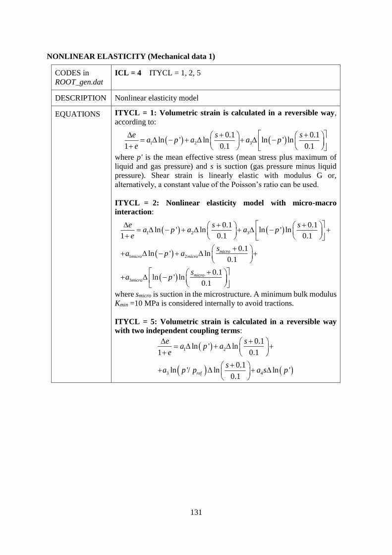
131
NONLINEAR ELASTICITY (Mechanical data 1)
CODES in
ROOT_gen.dat
ICL = 4 ITYCL = 1, 2, 5
DESCRIPTION Nonlinear elasticity model
EQUATIONS ITYCL = 1: Volumetric strain is calculated in a reversible way,
according to:
1 2 3
0.1 0.1ln ' ln ln ' ln
1 0.1 0.1
e s sa p a a p
e
where p' is the mean effective stress (mean stress plus maximum of
liquid and gas pressure) and s is suction (gas pressure minus liquid
pressure). Shear strain is linearly elastic with modulus G or,
alternatively, a constant value of the Poisson’s ratio can be used.
ITYCL = 2: Nonlinear elasticity model with micro-macro
interaction:
1 2 3
1 2
3
0.1 0.1ln ' ln ln ' ln
1 0.1 0.1
0.1ln ' ln
0.1
0.1ln ' ln
0.1
micromicro micro
micromicro
e s sa p a a p
e
sa p a
sa p
where smicro is suction in the microstructure. A minimum bulk modulus
Kmin =10 MPa is considered internally to avoid tractions.
ITYCL = 5: Volumetric strain is calculated in a reversible way
with two independent coupling terms:
1 2
3 4
0.1ln ' ln
1 0.1
0.1ln '/ ln ln '
0.1ref
e sa p a
e
sa p p a s p

132
PARAMETERS
NONLINEAR ELASTICITY. ITYCL = 1 (volumetric strain is calculated in a reversible way):
P1 a1 - = - /(1+e), where is the slope of the unload/reload curve in the (e - lnp')
diagram
P2 a2 - = - s/(1+e), where s is the slope of the unload/reload curve in the (e -
ln((s+0.1)/0.1)) diagram
P3 a3 - Coupling term
P4 G MPa Shear modulus (P4 > 0 requires P5 = 0)
P5 - Poisson’s ratio (P5 > 0 requires P4 = 0)
P6 tens MPa Tension term to avoid tractions (p’- tens 0)
P7 Kmin MPa Minimum bulk modulus
NONLINEAR ELASTICITY. ITYCL = 2 (nonlinear elasticity with micro-macro interaction)
P1 – P5 The same as in ITYCL = 1
P6 a1micro - Volumetric deformation associated to microstructure
P7 a2micro - Volumetric deformation associated to microstructure
P8 a3micro - Volumetric deformation associated to microstructure
P9 Term of interchange of water between micro and macro
structures of deformation
P10 Initial smicro MPa Initial suction of the micro structure
Suction micro is used as history variable and, therefore, the model cannot be combined with
viscoplastic models.
NONLINEAR ELASTICITY. ITYCL = 5 (with two independent coupling terms)
P1 – P7 The same as in ITYCL = 1
P8 a4 MPa-1 Coupling term
P9 pref MPa Reference pressure

133
ANALOGY WITH BBM
Elastic part of BBM (isothermal):
( ) ( ', )'
1 ' 1 0.1
e i sv
s p sdp dsd
e p e s
where:
( ) 1i io is s ( ', ) 1 ln ' exps so sp ref s sp s p p s
For a3 = 0, the model (ITYCL=1) coincides with the elastic part of BBM for constant
coefficients:
0 01 2
0.1 0.1ln ' ln ln ' ln
1 0.1 1 1 0.1
i se s sa p a p
e e e
For a3 different from zero the equation ( ITYCL=1) can be expanded in the following way.
1 2 3
1 3 2 3
3 31 2
1 2
0.1 0.1ln ' ln ln ' ln
1 0.1 0.1
0.1 0.1ln ln ' ln ' ln
0.1 0.1
0.1 0.11 ln ln ' 1 ln ' ln
0.1 0.
e s sa p a a p
e
s sa a p a a p
a as sa p a p
a a
1
Depending on the values of the parameters, negative compressibility can be obtained. This
can be limited with the Kmin indicated above.
For a3 and a4 different from zero the equation (ITYCL=5) can be transformed in the following
way.
1 2 3 4
1 4 2 3
341 2
1 2
0.1 0.1ln ' ln ln '/ ln ln '
1 0.1 0.1
0.1ln ' ln ' ln
0.1
0.11 ln ' 1 ln '/ ln
0.1
ref
ref
e s sa p a a p p a s p
e
sa a s p a a p
aa sa s p a p p
a a
0 0
1 2 4 1 3 2 1 1
i si spa a a a a a
e e
_______________________________________

134
CORRESPONDANCE WITH LINEAR ELASTICITY PARAMETERS
Linear elasticity using volumetric and shear moduli:
𝑑휀𝑣 =𝑑𝑝′
𝐾 𝑑휀𝑑 =
𝑑𝑞
2𝐺
Bulk and shear elastic parameters as a function of Young and Poisson parameters:
𝐾 =𝐸
3(1 − 2𝜈) 𝐺 =
𝐸
1 + 𝜈
A typical non-linear elasticity model proportional to mean effective stress, can be compared
with linear elasticity if the tangent moduli are calculated (for compression negative):
𝑑휀𝑣𝑑𝑝′
=𝑎1 + 𝑎3 ln(𝑠)
𝑝′=1
𝐾 ⇒ 𝐾 =
𝑝′
𝑎1 + 𝑎3 ln(𝑠)> 𝐾𝑚𝑖𝑛
For constant Poisson ratio 𝜈 the following equivalences can be used:
𝐸 = 3𝐾(1 − 2𝜈) = 3(1 − 2𝜈)𝑝′
𝑎1 + 𝑎3 𝑙𝑛(𝑠)> 3(1 − 2𝜈)𝐾𝑚𝑖𝑛
𝐺 =3(1 − 2𝜈)
1 + 𝜈
𝑝′
𝑎1 + 𝑎3 𝑙𝑛(𝑠)>3(1 − 2𝜈)
1 + 𝜈𝐾𝑚𝑖𝑛
In case that a constant shear modulus G is given instead of 𝜈, then:
𝜈 =3𝐾 − 2𝐺
2(3𝐾 + 𝐺)=
3𝑝′
𝑎1+𝑎3 𝑙𝑛(𝑠)− 2𝐺
2(3𝑝′
𝑎1+𝑎3 𝑙𝑛(𝑠)+ 𝐺)
>3𝐾𝑚𝑖𝑛 − 2𝐺
2(3𝐾𝑚𝑖𝑛 + 𝐺)
𝐸 =9𝐾𝐺
3𝐾 + 𝐺=
9𝑝′
𝑎1+𝑎3 𝑙𝑛(𝑠)𝐺
3𝑝′
𝑎1+𝑎3 𝑙𝑛(𝑠)+ 𝐺
>9𝐾𝑚𝑖𝑛𝐺
3𝐾𝑚𝑖𝑛 + 𝐺
In case that a material with a Young’s Modulus changing with stress has to be modelled, the
following equation can be used (without suction effects):
𝐸 =3(1 − 2𝜈)𝑝′
𝑎1 and 𝐸𝑚𝑖𝑛 = 3𝐾𝑚𝑖𝑛(1 − 2𝜈)
Note that in this model implementation, 𝑎1 must be input as a negative value.
_______________________________________

135
VISCOELASTICITY - CREEP (Mechanical data 1)
CODES in
ROOT_gen.dat
ICL = 2 ITYCL = 1, 2, 4, 6, 11, 12
DESCRIPTION Parameters for linear viscous deformation model.
EQUATIONS ITYCL = 1: FADT for saline materials
The deformation mechanism fluid assisted diffusional transfer
(FADT) was applied to develop an equation for creep of salt under
wet conditions.
Strain rate for a linear viscoelasticity is computed as:
d
dt =
1
2( - p )+
1
3p
FADT
FADT
d
FADT
v
I I
where ’ is the effective stress tensor ( ’ = + Pf, where Pf =
max(Pg, Pl)), p’ is the mean effective stress (p' = p + Pf), I is the
identity tensor.
Volumetric and deviatoric viscosities are defined as:
1 16
1
2
16
0
3
0
3
FADT
v
l
FADT
v
FADT
d
l
FADT
d
B T S
dg e
B T S
dg e
( )( )
( )( )
where gFADTd(e) and gFADT
v(e) are internal nonlinear functions of
void ratio (e), and Sl is degree of saturation.
B TA
RT
Q
RT
B B( ) exp
g eg e
eg e
g
eFADT
v
FADT
d( )( )
( )( )
/
3
1 1
2 3 2 2
)1)(1(3
2
)1(
12/32 ee
ef
fg
ITYCL = 2, 4: Constant viscosity plus degree of saturation effect
Strain rate for a linear viscoelasticity is computed as:
𝑑𝛆
𝑑𝑡= (
1
2𝜂𝑑(𝜎′ − 𝑝′𝐈) +
1
3𝜂𝑣𝑝′𝐈) 𝑓(𝑆𝑙)
where ’ is the effective stress tensor ( ’ = + Pf, where Pf =
max(Pg, Pl)), p’ is the mean effective stress (p' = p + Pf), I is the
identity tensor. For ITYCL=2 the degree of saturation function is
calculated as 𝑓(𝑆𝑙) = √𝑆𝑙 while for ITYCL=4 the degree of
saturation is not considered, i.e. 𝑓(𝑆𝑙) = 1.

136
CODES in
ROOT_gen.dat ICL = 2 ITYCL = 1, 2, 4, 6, 11, 12
DESCRIPTION Parameters for linear viscous deformation model.
EQUATIONS ITYCL = 6: Secondary consolidation for unsaturated soils
Strain rate for a linear viscoelasticity is computed as:
𝑑𝛆
𝑑𝑡= (
1
2𝜂𝑑(𝜎′ − 𝑝′𝐈) +
1
3𝜂𝑣𝑝′𝐈)
where
1
𝜂𝑣= 𝐴 (1 − 𝛽 log (
𝑠 + 0.1
0.1))
1
𝑡 − 𝑡0𝜂𝑑 = 𝐵𝜂𝑣
where t is time in seconds, 𝑡0 is a reference time and s is suction.
ITYCL = 11: Kelvin model
The Kelvin viscoelastic model can simulate the primary creep stage
of rocks. The strain rate for linear viscoelasticity using the Kelvin
model is computed as:
𝑑𝛆
𝑑𝑡= 𝐂v (− )
where Cv represents the compliance matrix of the viscous dashpot.
The Kelvin model can be combined with the elastic model, to be the
Generalized Kelvin model.
ITYCL = 12: Viscous dashopt combined with Kelvin model
This model can simulate the primary and secondary creep stages of
rocks. Strain rate this model is computed as:
𝑑𝛆
𝑑𝑡=
M
+ 𝐂v (− )
This model can be combined with the elastic model, to become the
Burgers model.

137
PARAMETERS FOR ITYCL = 1 (Mech. data 1 ─ Viscoelasticity - Creep)
P1 do m Grain size
P2 AB m3 s-1 MPa-1 Pre-exponential parameter
P3 QB J mol-1 Activation energy
If the pre-exponential parameter is set to zero (AB = 0.0) the viscous counterpart of the model
does not work. In this way the parameter acts as option because the value of these pre-
exponential parameter is checked to decide if this mechanism is considered.
This viscoelastic model (corresponding to FADT mechanism of deformation) requires that the
liquid pressures are computed or, alternatively, a value of PLCONS greather that -10-12 MPa.
Otherwise, liquid is considered inexistent and the mechanism FADT remains inactive.
PARAMETERS FOR ITYCL = 2, 4 (Mech. data 1 ─ Viscoelasticity - Creep)
P1 𝜂𝑣 MPa s Volumetric viscosity
P2 𝜂𝑑 MPa s Deviatoric viscosity
PARAMETERS FOR ITYCL = 6 (Mech. data 1 ─ Viscoelasticity - Creep)
P1 𝐴 MPa-1 s-1 Parameter for volumetric viscosity
P2 𝛽 (-) Parameter for suction dependence
P3 𝑡0 s Reference time
P4 Void
P5 B (-) Parameter for deviatoric viscosity (infinity for no
deviatoric viscous deformation)
PARAMETERS FOR ITYCL = 11 (Mech. data 1 ─ Viscoelasticity - Creep)
P1 EK MPa Elastic modulus of the elastic spring
P2 K (-) Possion’s ratio of the elastic spring
P3 Kv MPa s Volumetric viscosity of the viscous dashpot
P4 Kd MPa s Deviatoric viscosity of the viscous dashpot
PARAMETERS FOR ITYCL = 12 (Mech. data 1 ─ Viscoelasticity - Creep)
P1 Mv MPa s Volumetric viscosity of the viscous dashpot (
M𝑣 )
P2 Md MPa s Deviatoric viscosity of the viscous dashpot (
M𝑑 )
P3 EK MPa Same as P1 of ITYCL = 11
P4 K (-) Same as P2 of ITYCL = 11
P5 Kv MPa s Same as P3 of ITYCL = 11
P6 Kd MPa s Same as P4 of ITYCL = 11

138
VISCOPLASTICITY - CREEP (Mechanical data 1)
CODES in
ROOT_gen.dat
ICL = 3 ITYCL = 1
DESCRIPTION The deformation mechanism referred as dislocation creep (DC)
has been applied to develop an equation for creep of porous salt
aggregates. This mechanism leads to nonlinear dependences on
stresses.
EQUATIONS Strain rate for a nonlinear viscoelasticity is computed as:
d
dt =
1
d(F)
G
DC
DC
where G is a flow rule, F is a stress function and is a scalar
function. These functions are defined as: 12
12 ( ) =
v n+n DC
p d
p DC
pF G q F F
1( ) ( )v
DCv
DC
A T g e
1
( ) ( )d
DCd
DC
A T g e
where n is the power that comes from the rock power law and
gDCd(e) and gDC
v(e) are internal nonlinear functions of void ratio
(e) defined as follows:
( ) 3( 1) v n
DCg e g f
gf
gggeg
n
dDC
1
3
12
3
1)(
12
where f and g are functions of the void ratio (see expression in
the constitutive law Viscoelasticity for saline materials).
The temperature dependence is considered as:
A T AQ
RTA
A( ) exp
PARAMETERS
P1 AA s-1 MPa-n Pre-exponential parameter
P2 QA J m-1 Activation energy
P3 n - Stress power
P4 – P10 Void
If the pre-exponential parameter is set to zero the viscous counterpart of the model does not
work. In this way the parameter acts as option because the value of this pre-exponential
parameter is checked to decide if this part of the model is operating.

139
CODES in
ROOT_gen.dat ICL = 3 ITYCL = 3
DESCRIPTION Viscoplastic constitutive equation based on a single internal state
variable which is a function of plastic work are used to calculate the
response of copper to change of strain rate over a range of temperatures.
EQUATIONS Starting with the Prandtl-Reuss-Von Mises law of isotropic plasticity:
p
ij ijs (1)
Where 휀�̇�𝑗𝑝
and Sij are the deviatoric plastic strain rate and the stress,
respectively. Squaring equation (1) gives:
2
2 2
p
JD
2
2 0
21
exp
23
n
p n
n
zD D
J
(2)
Where 𝐷2𝑃 is the second invariant of the plastic strain rate, and J2
is the
second invariant of the stress deviator.
Combining equation 1 and 2, the plastic strain takes the form:
0
2
21
exp2
23
n
p ij
ij
n
n
z SD
JJ
𝑛 = (835 + 5𝑇(𝐾))/𝑇(𝐾)
𝑇(𝐾) = 𝑇(𝐶) + 273.15
The parameter Z in the equation can be interpreted as an internal state
variable which provides a measure of the overall resistance to plastic
flow, and n is a strain rate sensitivity parameter.
1 1 0( )exp pZ Z Z Z mw 0 1 exp pm m m w
The corresponding form is then based on the concept that plastic work,
𝑤𝑝, controls the hardening process, and that the plastic work and its time
derivative are function of 𝜎𝑖𝑗 and 휀�̇�𝑗𝑝
.
p
p ij ijw
PARAMETERS
P1 D0 s-1 Limiting strain rate (usually D0 = 104 s-1 for copper)
P2 Z0 MPa Initial value of the internal state variable Z (typically Z0 = 31 MPa)
P3 Z1 MPa Saturated value of the internal state variable Z (typically Z0 = 237
MPa for copper)
P4 mo (MPa)-1 Initial value of hardening parameter (typically mo = 0.15 MPa for
copper)
P5 m1 (MPa)-1 Saturated value of hardening parameter (typically m1 = 0.25 MPa for
copper)
P6 α (MPa)-1 A material constant (typically α = 0.5 MPa for copper)
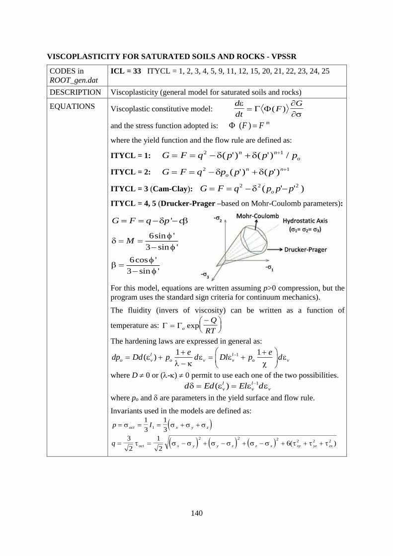
140
VISCOPLASTICITY FOR SATURATED SOILS AND ROCKS - VPSSR
CODES in
ROOT_gen.dat
ICL = 33 ITYCL = 1, 2, 3, 4, 5, 9, 11, 12, 15, 20, 21, 22, 23, 24, 25
DESCRIPTION Viscoplasticity (general model for saturated soils and rocks)
EQUATIONS Viscoplastic constitutive model: d
dtF
G
( )
and the stress function adopted is: ( ) mF F
where the yield function and the flow rule are defined as:
ITYCL = 1: G F q p p pn n
o 2 1 ( ') ( ') /
ITYCL = 2: G F q p p po
n n 2 1 ( ') ( ')
ITYCL = 3 (Cam-Clay): G F q p p po 2 2 2 ( ' ' )
ITYCL = 4, 5 (Drucker-Prager –based on Mohr-Coulomb parameters):
'G F q p c
6sin '
3 sin 'M
6cos '
3 sin '
For this model, equations are written assuming p>0 compression, but the
program uses the standard sign criteria for continuum mechanics).
The fluidity (invers of viscosity) can be written as a function of
temperature as:
o
Q
RTexp
The hardening laws are expressed in general as:
11 1( )l l
o v o v v o v
e edp Dd p d Dl p d
where D 0 or (-) 0 permit to use each one of the two possibilities. 1( )l l
v v vd Ed El d
where po and are parameters in the yield surface and flow rule.
Invariants used in the models are defined as:
p I
q
oct x y z
oct x y y z z x xy yz zx
1
3
1
3
3
2
1
26
1
2 2 22 2 2( )

141
CODES in
ROOT_gen.dat
ICL = 33 ITYCL = 1, 2, 3, 4, 5, 9, 11, 12, 15, 20, 21, 22, 23, 24, 25
DESCRIPTION Viscoplasticity (general model for saturated soils and rocks)
EQUATIONS ITYCL = 9: For rock salt with dilatancy:
1 1
for 0 0 for 0m
F a q bp G a q bp
F F F F F
0.250.25
3 2 4 0
2
5 6 7 0
d d d
d d d d d
b a a W a W W
a a W a W W dW qd
From a numerical point of view it is set 6 7a a
ITYCL = 11: Mohr-Coulomb (MC) model with dilatancy:
2
1sin (cos sin sin ) cos
3F p J c
2
1sin (cos sin sin ) cos
3G p J c
for 0 0 for 0mF F F F F
This model uses the standard sign criteria for continuum mechanics,
and equations are written assuming p>0 tension. is the dilatancy
angle and is a parameter for the plastic potential.
Invariants used in the models are defined as:
1
2 2 2 2 2 2
2
1 3
3
2
1 1
3 3
1 16( )
2 6
1 3 3sin ( ), 30 30
3 2
x y z
ij ij x y y z z x xy yz zx
p I
J S S
J
J
Where2 2 2
3 2x y z xy yz zx x yz y xz z xyJ S S S S S S .
To avoid numerical issues, the corners of the MC yield surface are
rounded by introducing T . The rounded yield surface is as follows:
2sin cosFF p J K c
sin 3 ,
1cos sin sin ,
3
T
F
T
A B
K

142
13 tan tan 31
3cos3
tan 3 3tan sin
T T
T
T T
signA
1 1
sin sin cos3 cos3 3
T T
T
B sign
1, 0
1, 0sign
For the numerical calculation, a hyperbolic yield surface is
adopted, as follows:
2 2 2
2 sin sin cosFF J K a p c
Where: cotmca m c
The closer to 0 is the value of mmc, the closer would be the
hyperbolic surface to the actual MC surface, as shown in the
following figure:

143
CODES in
ROOT_gen.dat
ICL = 33 ITYCL = 1, 2, 3, 4, 5, 9, 11, 12, 15, 20, 21, 22, 23, 24, 25
DESCRIPTION Viscoplasticity (general model for saturated soils and rocks)
EQUATIONS ITYCL = 12: MC model with dilatancy and strain-softening:
2
1sin cos sin sin cos
3F p J c
2
1sin (cos sin sin ) cos
3G p J c
for 0 0 for 0mF F F F F
Similar model to ITYCL=11, but in this case both the cohesion and the
friction angle depend on the softening parameter ,
*
*
*
, 0
, 0
,
peak
res peakpeak
res
k
k kk k
k
Where kpeak and kres are peak and residual values of k, respectively; k
represents both cohesion c and friction angle . is defined as the
value of the softening parameter controlling the transition between the
softening and residual stages.
The expression of the softening parameter is the following:
2 2 2
2 2 23
1 1 12
2 2 2
p p p p p p
x m y m z m
p p p
xy yz zx
Where 1
3
p p p p
m x y z .
The corners of MC yield surface are rounded by introducing T . The
rounded method is the same as in ITYCL=11, but the rounded parameters
T and mcm are fixed at 25 and 0.25 in this model.

144
CODES in
ROOT_gen.dat
ICL = 33 ITYCL = 1, 2, 3, 4, 5, 9, 11, 12, 15, 20, 21, 22, 23, 24, 25
DESCRIPTION Viscoplasticity (general model for saturated soils and rocks)
EQUATIONS ITYCL = 15: MC model with anisotropic behaviour:
The stress space in the global coordinate system (global
) can be transferred
to the local one (local
), using the transformation matrix a. Moreover, the
anisotropic stress space (ani
) can be obtained by introducing the stresses
scaling factor (CN and C
T):
local global Tσ aσ a
local local local
11 N 12 T 13
ani local local local
12 22 N T 23
local local local
T 13 T 23 N 33
C C
C C
C C C
σ
where a =
cos cos sin cos sin
sin cos cos sin sin
sin 0 cos
with [deg] rotating around z-axis, and then, [deg] rotating around the
y-axis.
Then, the anisotropic Mohr-Coulomb failure behaviour model can be
expressed in the anisotropic stress space (ani
):
ani ani ani ani ani
MC 2
1sin cos sin sin cos
3F p J c
ani ani ani ani ani
MC 2
1sin cos sin sin
3G p J
No dilatation is considered (i.e. = 0) because of the adopted perfectly-
plastic post-failure behaviour model. is a parameter for the plastic
potential.
Invariants used in the models are defined as:
ani ani ani ani
x y z
ani ani ani
2
2 2 2ani ani ani ani ani ani ani ani ani ani ani ani ani
3
aniani 1 3
3ani
2
1
3
1
2
2
1 3 3sin ( )
3 2
ij ij
x y z xy yz zx x yz y xz z xy
p
J S S
J S S S S S S
J
J
This model is based in Mánica M, Gens A, Vaunat J, et al. A cross-
anisotropic formulation for elasto-plastic models. Géotechnique Letters,
2016, 6(2): 156-162.

145
CODES in
ROOT_gen.dat
ICL = 33 ITYCL = 1, 2, 3, 4, 5, 9, 11, 12, 15, 20, 21, 22, 23, 24, 25
DESCRIPTION Viscoplasticity (general model for saturated soils and rocks)
EQUATIONS ITYCL = 20: Hoek-Brown (HB) model with dilatancy:
2
2 2
4 2cos cos
63
hb cihb hb
ci hb
sF J m J m p
m
2
1sin (cos sin sin )
3G p J
for 0 0 for 0mF F F F F
This model uses the standard sign criteria for continuum mechanics, and
equations are written assuming p>0 tension; hbm and hbs are parameters
of HB failure criterion. ci is the compressive strength of intact rock
mass. is the dilatancy angle and is a parameter for the plastic
potential.
For this model, the corners of HB yield surface are rounded by
introducing T . The rounded yield surface is as follows:
2hb ci
F hb
hb
sF K J m p
m
2
2
sin 3 , 30
4 2cos cos ,
63
sin 3 , 30
T
F hb T T
ci
T
A B
K J m
A B
where:
2
2
2
sin cos 1cos sin tan 3
33 3 3
4 cos 8 sin cos tan 3
3
8 sin cos cossin
3 cos3 3cos3 3
T Thb T T T
T T T T
ci ci
hbT T TT
ci T T
A m
J
mB J
2
2
2
sin cos 1cos sin tan 3
33 3 3
4 cos 8 sin cos tan 3
3
8 sin cossin
3 cos3 3cos3 3
T Thb T T T
T T T T
ci ci
hbT TT
ci T T
A m
J
mB J

146
CODES in
ROOT_gen.dat
ICL = 33 ITYCL = 1, 2, 3, 4, 5, 9, 11, 12, 15, 20, 21, 22, 23, 24, 25
DESCRIPTION Viscoplasticity (general model for saturated soils and rocks)
EQUATIONS ITYCL = 21: HB model with dilatancy and strain-softening:
2
2 2
4 2cos cos
63
hb
ci
hb ci
hb
hb
F J m J
sm p
m
2
1sin (cos sin sin )
3G p J
for 0 0 for 0mF F F F F
Similar model to ITYCL=20, but in this case both the parameters of
Hoek-Brown failure criterion, hbm and hbs , are functions of the
softening parameter :
*
*
*
, 0
,0
,
peak
res peakpeak
res
k
k kk k
k
Where peakk and
resk are peak and residual value of k, respectively; k
represents both mhb and shb. is defined as the value of the softening
parameter controlling the transition between the softening and residual
stages. The expression for the softening parameter is:
2 2 2
2 2 23
1 1 12
2 2 2
p p p p p p
x m y m z m
p p p
xy yz zx
Where 1
3
p p p p
m x y z .
The corners of strain-softening HB yield surface are rounded by
introducing T . The rounded method is the same as in ITYCL=20, but
the rounded parameter T is fixed at 25 in this model.

147
CODES in
ROOT_gen.dat ICL = 33 ITYCL = 1, 2, 3, 4, 5, 9, 11, 12, 15, 20, 21, 22, 23, 24, 25
DESCRIPTION Viscoplasticity (general model for saturated soils and rocks)
EQUATIONS ITYCL = 22: HB model with dilatancy:
2
2 2
4 2cos cos
63
hb
ci
hb cihb
hb
F J m J
sm p
m
2
2 2
4 2cos cos
63
hb
ci
hb cihb
hb
G J m J
sm p
m
for 0 0 for 0mF F F F F
Similar model to ITYCL=20, except for the form of the plastic potential
G. In this model, the expression forthe plastic potential is related to the
yield surface. It is considered an associated flow rule, i.e. F=G, when
equal to 1.
ITYCL = 23: HB model with dilatancy and strain-softening:
2
2 2
4 2cos cos
63
hb
ci
hb ci
hb
hb
F J m J
sm p
m
2
2 2
4 2cos cos
63
hb
ci
hb ci
hb
hb
G J m J
sm p
m
Similar model to ITYCL=21, except for the form of the plastic potential
G. In this model, the expression of the plastic potential is related to the
yield surface. It is considered an associated flow rule, i.e. F=G, when
equal to 1. In this model, both the yield surface and the plastic potential
depend on the softening parameter .

148
CODES in
ROOT_gen.dat ICL = 33 ITYCL = 1, 2, 3, 4, 5, 9, 11, 12, 15, 20, 21, 22, 23, 24, 25
DESCRIPTION Viscoplasticity (general model for saturated soils and rocks)
EQUATIONS ITYCL = 24: 3D Pan-Hudson simplified HB model (Pan &
Hudson, 1988):
2
2 2
3 3
2hb hb hb ci
ci
F m p J m J s
2
2 2
3 3
2hb hb hb ci
ci
G m p J m J s
for 0 0 for 0mF F F F F
This model uses the standard sign criteria for continuum mechanics,
and equations are written assuming p>0 tension; hbm and
hbs are
parameters of the HB failure criterion. ci is the compressive strength
of the intact rock mass. is the the dilatancy angle and is a
parameter for the plastic potential. It is considered associated flow
rule, when equal to 1.
ITYCL = 25: 3D Pan-Hudson simplified HB model (Pan &
Hudson, 1988) with strain-softening:
2
2 2
3 3
2hb hb hb ci
ci
F m p J m J s
2
2 2
3 3
2hb hb hb ci
ci
G m p J m J s
for 0 0 for 0mF F F F F
Similar model to ITYCL=24, but in this case both the parameters
of 3D Pan-Hudson simplified Hoek-Brown failure criterion, hbm
and hbs , are dependent on the softening parameter , following
the same relationships as in ITYCL=21.
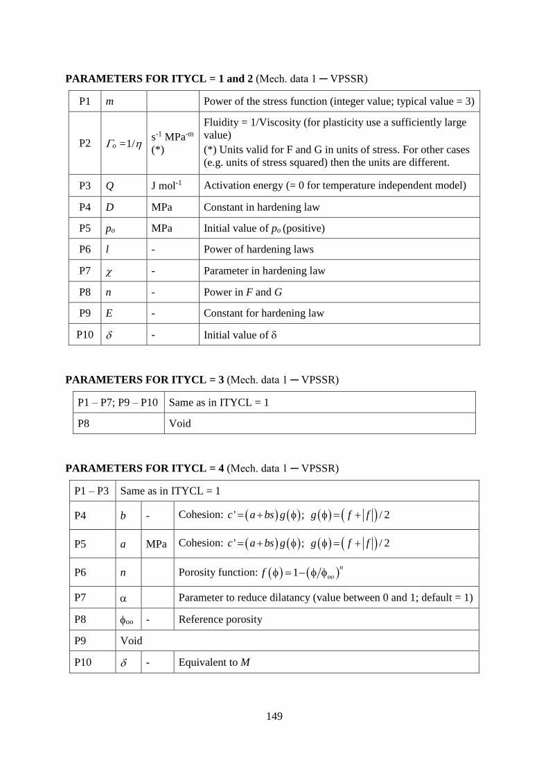
149
PARAMETERS FOR ITYCL = 1 and 2 (Mech. data 1 ─ VPSSR)
P1 m Power of the stress function (integer value; typical value = 3)
P2 o =1/ s-1 MPa-m
(*)
Fluidity = 1/Viscosity (for plasticity use a sufficiently large
value)
(*) Units valid for F and G in units of stress. For other cases
(e.g. units of stress squared) then the units are different.
P3 Q J mol-1 Activation energy (= 0 for temperature independent model)
P4 D MPa Constant in hardening law
P5 po MPa Initial value of po (positive)
P6 l - Power of hardening laws
P7 - Parameter in hardening law
P8 n - Power in F and G
P9 E - Constant for hardening law
P10 - Initial value of
PARAMETERS FOR ITYCL = 3 (Mech. data 1 ─ VPSSR)
P1 – P7; P9 – P10 Same as in ITYCL = 1
P8 Void
PARAMETERS FOR ITYCL = 4 (Mech. data 1 ─ VPSSR)
P1 – P3 Same as in ITYCL = 1
P4 b - Cohesion: ' ; / 2c a bs g g f f
P5 a MPa Cohesion: ' ; / 2c a bs g g f f
P6 n Porosity function: 1n
oof
P7 Parameter to reduce dilatancy (value between 0 and 1; default = 1)
P8 oo - Reference porosity
P9 Void
P10 - Equivalent to M

150
PARAMETERS FOR ITYCL = 5 (Mech. data 1 ─ VPSSR)
P1 – P3, P7, P10 Same as in ITYCL = 4
P4, P6, P8, P9 Void
P5 c MPa Cohesion
PARAMETERS FOR ITYCL = 9 (Mech. data 1 ─ VPSSR)
P1 – P3 Same as in ITYCL = 1
P4 a6
P5 Wd0
P6 a1
P7 a2
P8 a3
P9 a4
P10 a5
PARAMETERS FOR ITYCL = 11 (Mech. data 1 ─ VPSSR)
P1 – P3 Same as in ITYCL = 1
P4 Void
P5 c MPa Cohesion
P6 º Friction angle
P7 T º Lode angle value at which the corner smoothing function
starts (typical value –default*– = 25º)
P8 mcm (0 - 1)
Hyperbolic parameters for the yield surface. If mcm =0
then the failure surface would be the actual Mohr-
Coulomb failure surface (typical value –default*– = 0.25)
P9 (0 - 1) Parameter for the plastic potential (default* = 1)
P10 º Dilatancy angle (default* value = friction angle).
* Note that, in the case of parameters with default values, when setting them to zero –or to a
value lower than 10-25– automatically takes the default value. Hence, if the user actually wants
to set a parameter to zero, a low value but greater than 10-25 should be input.

151
PARAMETERS FOR ITYCL = 12 (Mech. data 1 ─ VPSSR)
P1 – P3 Same as in ITYCL = 1
P4 * Critical value of the softening parameter (corresponding
to the transition between softening and residual stages)
P5 cpeak MPa Peak cohesion
P6 peak º Peak friction angle
P7 cres MPa Residual cohesion (default* = peak cohesion)
P8 res º Residual friction angle (default* = peak friction angle)
P9 (0 - 1) Parameter for the plastic potential (default* = 1)
P10 º Dilatancy angle (default* value = peak friction angle)
* Note that, in the case of parameters with default values, when setting them to zero –or to a
value lower than 10-25– automatically takes the default value. Hence, if the user actually wants
to set a parameter to zero, a low value but greater than 10-25 should be input.
PARAMETERS FOR ITYCL = 15 (Mech. data 1 ─ VPSSR)
P1 – P3 Same as in ITYCL = 1
P4, P10 Void
P5 c MPa Cohesion
P6 º Friction angle
P7 CN Stress scaling factor
P8 CT Stress scaling factor
P9 (0 - 1) Parameter for the plastic potential (default = 1)
PARAMETERS FOR ITYCL = 20 (Mech. data 1 ─ VPSSR)
P1 – P3 Same as in ITYCL = 1
P4 Void
P5 mhb MPa Hoek-Brown parameter m
P6 shb Hoek-Brown parameter s
P7 ci MPa Compressive strength of the intact rock mass
P8 T º
Lode angle value at which the corner smoothing function
starts (typical value –default– = 25º)
P9 (0 - 1) Parameter for the plastic potential (default = 1)
P10 º Dilatancy angle

152
PARAMETERS FOR ITYCL = 21 (Mech. data 1 ─ VPSSR)
P1 – P3 Same as in ITYCL = 1
P4 * Critical value of the softening parameter (corresponding
to the transition between softening and residual stages)
P5 peak
hbm MPa Hoek-Brown parameter m (peak value)
P6 peak
hbs Hoek-Brown parameter s (peak value)
P7 res
hbm MPa Hoek-Brown parameter m (residual value)
P8 res
hbs Hoek-Brown parameter s (residual value)
P9 ci MPa Compressive strength of the intact rock mass
P10 º Dilatancy angle
PARAMETERS FOR ITYCL = 22, 24 (Mech. data 1 ─ VPSSR)
P1 – P9 Same as in ITYCL = 20
P10 Void
PARAMETERS FOR ITYCL = 23, 25 (Mech. data 1 ─ VPSSR)
P1 – P9 Same as in ITYCL = 21
P10 (0 - 1) Parameter for the plastic potential (default = 0)
HISTORY VARIABLES:
The VPSSR (ICL = 33) requires four history variables:
Hist_var 1 Po MPa Evolution of preconsolidation mean stress
Hist_var 2 0 Evolution of (parameter of the flow rule)
Hist_var 3 EDP Plastic deviatoric strain
Hist_var 4 EVP Plastic volumetric strain
The first two variables can be assigned as initial conditions on surfaces/volumes if an initial
particular distribution on the geometry is required. The procedure is the same as followed by
initial stresses as was described in chapter II. PREPROCESS, PROBLEM DATA, section
II.2.3.5.
If no value is assigned for the first two variables in conditions, internally, the program sets the
input parameters P5 (for Po*) and P10 (for 0) of the ICL = 33 (ITYCL = 1, 2 or 3), as initial
values.
The evolution of the four history variables can be visualized as an output in Post-process GID
interface.
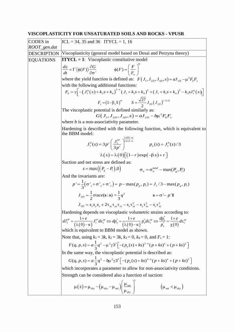
153
VISCOPLASTICITY FOR UNSATURATED SOILS AND ROCKS - VPUSR
CODES in
ROOT_gen.dat
ICL = 34, 35 and 36 ITYCL = 1, 16
DESCRIPTION Viscoplasticity (general model based on Desai and Perzyna theory)
EQUATIONS ITYCL = 1: Viscoplastic constitutive model
( ) ( )'
N
o
d G FF F
dt F
where the yield function is defined as: 2
1 2 3 2, , ,D D D b sF J J J s aJ F F
with the following additional functions:
2 20 0
1 2 4 1 1 4 1 1 4 3 1
n n
bF J s k s k J k s k J k s k k sJ s
3/ 2
3 2
271
2
m
s s D DF S S J J
The viscoplastic potential is defined similarly as:
2
1 2 3 2, , ,D D D b sG J J J s aJ b F F
where b is a non-associativity parameter.
Hardening is described with the following function, which is equivalent to the BBM model:
0 1 exps r s r
Suction and net stress are defined as:
And the invariants are:
1
1' ' ' ' max( , ) / 3 max( , )
3x y z g l g lp p p p J p p
2
2
2 2 2
3
1 1( : ) = ' '
2 3
2
D
D x y z xy yz zx x yz y xz z xy
J trace q p
J s s s s s s
s s s I
Hardening depends on viscoplastic volumetric strains according to:
*0* * * *
1 1 *
1 1 1
00 0
o vp vp vpov o o v v
o
dpe e edJ J d dp p d d
p
which is equivalent to BBM model as shown.
Note that, using k1 = 3k, k2 = 3k, k3 = 0, k4 = 0, and Fs = 1:
2 2 2 2 21( , , ) 3 ( ( ) ) ( ) ( )
3
n n
oF q p s a q p s ks p ks p ks
In the same way, the viscoplastic potential is described as:
2 2 2 2 21( , , ) 3 ( ( ) ) ( ) ( )
3
n n
oG q p s a q b p s ks p ks p ks
which incorporates a parameter to allow for non-associativity conditions.
Strength can be considered also a function of suction:
s
satdry dry sat sat dry
dry
s
(0)0* ( )
0 011 1( ) 3 ( ) ( ) / 3
3
sc
oc
JJ s p p s J s
p
max ,0g ls P P max( , )total
n n g lP P

154
PARAMETERS FOR ITYCL=1
ICL = 34 (Mechanical data 1 VPUSR 1) ITYCL = 1
P1 s-1 MPa-1 Fluidity = 1/Viscosity (for plasticity use a sufficiently
large value)
P2 N Power of the stress function (integer value)
P3 Fo MPa2 Fo = 1 MPa2
P4 exp(s)
P5 b Non associativity parameter.
ICL = 35 (Mechanical data 1 VPUSR 2) ITYCL = 1
P1 n - Power in F and G (integer value)
P2 - Parameter in F and G
P3 s - Typical value 0 (then Fs = 1, and J3D is not considered)
P4 m - Typical value -0.5, only required if s 0
P5 DRY - For some cases, = MDRY corresponding
approximately to Cam-Clay model.
P6 - -
P7 (J1o*)F MPa Positive value, initial size of F (note that this is the 1s
invariant)
P8 (J1o*)G MPa Positive value, initial size of G (note that this is the 1st
invariant)
P9 a - Parameter in F and G
P10 SAT - For some cases = MSAT corresponding
approximately to Cam-Clay model.
ICL = 36 (Mechanical data 1 VPUSR 3) ITYCL = 1
P1 - Elastic compression parameter
P2 - Viscoplastic compression parameter
P3 r - Parameter in LC curve
P4 - Parameter in LC curve
P5 pc MPa Parameter in LC curve
P6 k1 -
P7 k2 -
P8 k3 -
P9 k4 -

155
This model has the following case that can be used:
Cam-Clay model Cap models
a 3 3
n 1 3,5,7,9
-1/9 +1/9
k1
k2 -3k ?
k3 3k ?
k4 3ps0 ?
M M
Parameters k, ps0 (see BBM). M: slope of critical state line

156
VISCOPLASTICITY FOR UNSATURATED SOILS AND ROCKS - VPUSR
CODES in
ROOT_gen.dat
ICL = 34, 35, 36 (continued)
DESCRIPTION Viscoplasticity (general model for unsaturated soils based on Desai and
Perzyna theory).
EQUATIONS ICL = 36 (VPUSR 3), ITYCL = 2:
The LC curve is defined in the following way:
*
1 *
1 1
3 (0)( ) 3 3
( )
d o i
yo o
y yi d
p s JJ s J J J
s s
and the form of the compressibility is: 0 1 exps r s r
Hardening depends on viscoplastic volumetric strains according to:
0*
1
13
(0)
vp
v
io
dJ dk
ICL = 36 (VPUSR 3), ITYCL = 3:
The LC curve is defined in the following way:
0*
1 0*
1 1
3( ) 3 3
d i iyo
y yi d i d
p s JJ s p J p
s s
and the
form of the compressibility is: 0.1
( ); ( ) ln0.1
i d d d s
ss s s
Hardening depends on viscoplastic volumetric strains according to:
0*
1
13 vp
v
i io
dJ dk
For more details see Oldecop & Alonso, 2001.
ICL = 36 (Mechanical data 1 VPUSR 3); ITYCL = 2
P1 void -
P2 - Viscoplastic compression parameter
P3 r - Parameter in LC curve
P4 - Parameter in LC curve
P5 Jy MPa Parameter in LC curve
P6 k1 -
P7 k2 -
P8 k3 -
P9 k4 -
P10 aa -

157
ICL = 36 (Mechanical data 1 VPUSR 3); ITYCL = 3
P1 void -
P2 i- - Viscoplastic compression parameter
P3 d - Viscoplastic compression parameter
P4 s - Parameter (s) curve
P5 py MPa Parameter in LC curve
P6 k1 -
P7 k2 -
P8 k3 -
P9 k4 -
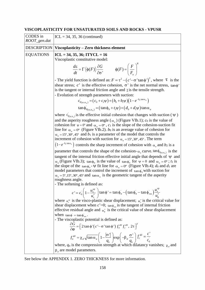
158
VISCOPLASTICITY FOR UNSATURATED SOILS AND ROCKS - VPUSR
See below the APPENDIX 1. ZERO THICKNESS for more information.
CODES in ROOT_gen.dat
ICL = 34, 35, 36 (continued)
DESCRIPTION Viscoplasticity – Zero thickness element
EQUATIONS ICL = 34, 35, 36; ITYCL = 16 Viscoplastic constitutive model:
( ) ( )'
N
o
d G FF F
dt F
- The yield function is defined as:
22 ' ' tan 'F c , where is the
shear stress; 'c is the effective cohesion, ' is the net normal stress, tan '
is the tangent or internal friction angle and is the tensile strength.
- Evolution of strength parameters with suction:
2 tan'
0 0 1 0 1,1 a
a
bc c c b b e
'
0 0 1 0 1,tan tan tan
aat d d
where '
0 , ac
is the effective initial cohesion that changes with suction ( )
and the asperity roughness angle (a ) (Figure VIb.1); c0 is the value of
cohesion for 0º and 0ºa , c1 is the slope of the cohesion-suction fit line for 0ºa (Figure VIb.2). b0 is an average value of cohesion for
15º,30º,45ºa and b1 is a parameter of the model that controls the increment of cohesion with suction for 15º,30º,45ºa . The term
2 tan1 ab
e
controls the sharp increment of cohesion with a and b2 is a
parameter that controls the shape of the cohesion-a curve.
'
0 ,tan
a is the
tangent of the internal friction effective initial angle that depends of and
a (Figure VIb.3); 0tan is the value of '
0tan for 0 and 0ºa ; t1 is the slope of the '
0tan - fit line for 0ºa (Figure VIb.4); d0 and d1 are model parameters that control the increment of '
0tan with suction for
5º,15º,30º ,45ºa and tan a is the geometric tangent of the asperity roughness angle. - The softening is defined as:
'
0 *' 1
vp
s
c
uc c
u
' ' '
0 0 *tan ' tan tan tan
vp
sres
u
u
where vp
su is the visco-plastic shear displacement; *
cu is the critical value for shear displacement when c’=0; 'tan res is the tangent of internal friction
effective residual angle and *u is the critical value of shear displacement
when ' 'tan tan res .
- The viscoplastic potential is defined as:
2 tan ' ' ' tan ' , 2T
dil dil
c
Gc f f
' '
tan 1 expdil
d a d
u u
fq q
'
0
'dil
c
cf
c
where, qu is the compression strength at which dilatancy vanishes; d and
d are model parameters.

159
Figure VIb.1. Effective cohesion vs. a (Zandarin, 2010)
Figure VIb.2. Effective cohesion vs. suction (Zandarin, 2010)
Figure VIb.3. Effective tangent of the internal friction angle vs. a (Zandarin, 2010)
Figure VIb.4. Effective tangent of the internal friction angle vs.suction (Zandarin, 2010)

160
PARAMETERS FOR ITYCL=16
ICL = 34 (Mechanical data 1 VPUSR 1); ITYCL = 16
P1 c0 MPa Initial cohesion
P2 0 º Initial friction angle
P3 -
P4 res º Residual friction angle
P5 *
cu m Critical value of shear displacement for cohesion
P6 *u m Critical value of shear displacement for friction
P7 d - Model parameter for dilatancy function
P8 d - Model parameter for dilatancy function
P9 a º Joint asperity angle
P10 qu MPa Compression strength for which dilatancy vanishes
ICL = 35 (Mechanical data 1 VPUSR 2); ITYCL = 16
P1-P2 -
P3 1/s Fluidity
P4 N Power of the stress function (integer value)
P5 F0 MPa F0=1 MPa (Default value)
ICL = 36 (Mechanical data 1 VPUSR 3); ITYCL = 16
P1 c1 MPa Model parameter for evolution of cohesion with suction
P2 b0 MPa Model parameter for evolution of cohesion with suction
P3 b1 - Model parameter for evolution of cohesion with suction
P4 b2 - Model parameter for evolution of cohesion with suction
P5 t1 - Model parameter for evolution of friction angle with suction
P6 d0 - Model parameter for evolution of friction angle with suction
P7 d1 - Model parameter for evolution of friction angle with suction
P8 a º Joint asperity angle

161
HISTORY VARIABLES:
The VPUSR model (ICL = 34, 35, 36) requires four history variables:
Hist_var 1 (J1o*)F MPa Evolution of size of F (note that this is the 1s invariant)
Hist_var 2 (J1o*)G MPa Evolution of size of G (note that this is the 1st invariant)
Hist_var 3 EDP Plastic deviatoric strain
Hist_var 4 EVP Plastic volumetric strain
The first two variables can be assigned as initial conditions on surfaces/volumes if an initial
particular distribution on the geometry is required. The procedure is the same followed by initial
stresses as was described in chapter II. PREPROCESS, PROBLEM DATA, section II.2.3.5.
If no value is assigned for the first two variables in conditions, internally, the program sets the
input parameters P7 (for (J1o*)F) and P8 (for (J1
o*)G) of the ICL=35 (ITYCL=1), as initial
values.
The evolution of the four history variables can be visualized as an output in Post-process GID
interface.
Note: Effective stresses plotted in the Post-process GID interface correspond with net stresses
for unsaturated conditions and Terzaghi's effective stresses for saturated conditions. Stress and
strain invariants follow the soil mechanics notation (positive for compression).

162
APPENDIX 1. ZERO THICKNESS
MECHANICAL PROBLEM
The mechanical behaviour of the joint elements is defined by the relation between stress and
relative displacements of the joint element (Figure VIb.5) calculated on the mid-plane. The
mid-plane relative displacements are interpolated using the nodal displacements and the shape
functions.
Figure VIb.5. Joint element with double nodes. a) Stress state on the mid-plane of the joint
element. b) Relative displacement defined at mid plane.
The normal and shear displacement increment calculated on the midplane is defined as:
4 4
n u
mp mp j
s mp
u
u
w r N I I u
where un and us are the normal and tangential relative displacements, r is a rotation matrix, Nmpu
is a matrix of shape functions, I4 is an identity matrix of 4th order, uj is the vector of nodal
displacements.
The stress tensor on the mid-plane is calculated as a function of displacement components,
normal and shear: '
'
mp mp
mp
σ D w
where ’mp is the net effective stress on the mid-plane of the element and it is defined as ’mp
= mp- max(Pg; Pl) mp; (is total mean stress; Pg is the gas pressure and Pl is the liquid
pressure, both interpolated to the mid-plane of the element); is the tangential stress on the
mid-plane; D is the stiffness matrix which relate relative displacements with the stress state.
MECHANICAL MODEL BASED ON ELASTO-VISCOPLASTIC FORMULATION
An elasto-viscoplastic formulation is proposed to model the mechanical behaviour of joints.
This formulation based on the development done by Perzyna (1963), Zienkiewicz et al. (1974),
Lorefice et al., (2007) allows the treatment of non-associated plasticity and strain softening
behaviour of joints subjected to shear displacements. More over, using the viscoplasticity it is
possible considered the variation of the strain rate with time.
The total displacements w are calculated by addition of reversible elastic displacements, we,
and viscoplastic displacements wvp, which are zero when stresses are below a threshold value
(the failure surface): w = we + wvp
The displacements are represented by a vector of two quantities in two-dimensional case and
have the following components:
,T
n su uw 3.22
1 2
3 4
mp1 mp2
ut
dl
a0a
un

163
ELASTIC BEHAVIOUR
The elastic behaviour of the joint is established as a relationship between the normal-tangencial
effective (’,) and the normal-tangential (un, us) relative displacement of the joint element.
This is established using a normal (Kn) and a tangential stiffness (Ks) coefficients. The normal
stiffness depends on the opening of the joint.
0'
0
n n
s s
K u
K u
constant ,min
sn Kaa
mK
where m is a parameter of the model; a is the opening or aperture of the element and amin is
the minimum opening or aperture of the element.
Figure VIb.6. Elastic constitutive law of the joint element. Normal stiffness depends on joint
opening.
VISCO-PLASTIC BEHAVIOUR
The constitutive behaviour for the mechanical of rough rock joint was developed based on the
formulations proposed by Gens, et al. (1985) and Carol, et al, (1997). According to these
theories, it is necessary to define a yield surface, a plastic potential and a softening law to
mathematical model the shear behaviour of a joint.
The visco-plastic displacements occur when the stress state of the joint reaches a failure
condition. The failure surface can be defined linearly (the one implemented in
CODE_BRIGHT):
22 ' ' tan 'F c
Or with hyperbolic shape (based on work done by Gens et al., (1990)):
222 'tan''tan'' ccF
where is the shear stress; c’ is the effective cohesion; ’is the net normal stress and tan’ is
the tangent of effective angle of internal friction. is a parameter.
'
amin a

164
Figure VIb.7. Hyperbolic (continuous) and linear (dashed) failure surface and strength
parameters
SOFTENING LAW
The strain-softening behaviour of the joint subjected to shear stress is modelled considering the
degradation of the strength parameters tan’ and c’.
The degradation of the parameters tan’ and c’ is considered dependent on the accumulated
viscoplastic shear displacement. This is based on the slip weakening model introduced by
Palmer & Rice (1973). In this way the tangent of the friction angle decays from the peak (intact
material) to the residual value and the cohesion from the value c to zero. Two different values
u* permit to define the decrease of cohesion (u*c’) and friction angle (u*tanФ’). The
mathematical expressions are:
0 *
u' ' 1
u
vp
s
c
c c
where c’ is the effective cohesion that corresponds to the visco-plastic shear displacement usvp;
c’0 is the initial value of the effective cohesion; u*c is a parameter.
0 0 *
utan ' tan ' tan ' tan '
u
vp
sres
tan’ is the tangent of effective angle of internal friction that corresponds to the visco-plastic
shear displacement usvp; tan’0, tan’res and u* are parameters.
Figure VIb.8 a) Evolution of the failure surface during softening. b) Softening law of cohesion.
c) Softening law of tan.
VISCO-PLASTIC DISPLACEMENTS
c
F=0
F<0
F>0
0
170°
res
1
2
c tan
us
c0
uc*
tan0
tanres
vp usvputan*
11
2
2

165
A viscoplastic yield surface implies that when F < 0 the stress state of the element falls inside
of the elastic region. In contrast, if F >= 0 the displacements of the element undergo a visco-
plastic component. The viscoplastic displacements are calculated as:
0
vpd F G
dt F
w
σ
where is a fluidity parameter. The visco-plastic displacement rate is given by a power of
law considered for the function :
vp N
n
Gu F t
vp N
s
Gu F t
PLASTIC POTENTIAL SURFACE AND DILATANCY
To calculate the direction of displacements it is necessary to define the derivatives of G with
respect to stresses:
2 tan ' ' ' tan ' , 2T
dil dil
c
Gc f f
σ
This is a non-associated flow rule, because of the inclusion of both parameters fdil and fcdil
which consider the dilatant behaviour of the joint with shear stresses (Lopez, et al. 1999). The
amount of dilatancy depends on the level of the normal stress and on the degradation of the
joint surface.
The following expressions describe these effects:
' '1 expdil
d
u u
fq q
0
'
'
dil
c
cf
c
Where qu, d are model parameters, c’ is the cohesion value that correspond to the visco-plastic
shear displacement usvp ; and c0’ is the initial value of the cohesion.
Then, the tangent visco-plastic compliance matrix is calculated as:
vp vp
n n
vp
vp vp
s s
u u
Cu u
21
2
2 tan ' ' ' tan '
2 tan '
vpN dil diln
c
N dil dil
c
uN F f f c t
F f f t
12 2 tan ' ' ' tan 'vp
N dil dilnc
uN F f f c t

166
12 2 tan ' ' ' tan 'vp
NsuN F c t
12 2vp
N NsuN F t F t
Finally, the elasto-viscoplastic mechanical model of the joint is expressed by the tangent
stiffness matrix:
1evp e vp
D C C
More information about this joint element can be found in Zandarin (2010) –see References.
APPENDIX 2. EXAMPLE OF USE
The use of the BBM model can be achieved by combination of the non-linear elasticity and the
viscoplasticity for unsaturated soils.
total elastic viscoplastic
The elastic part can be linear or nonlinear and may depend on suction and temperature. The
viscoplastic part can also be a function of suction.
The following parameters are required and example values are given:
NONLINEAR ELASTICITY. ITYCL = 1
P1 a1 - = - /(1+e), where is the slope of the unload/reload
curve in the (e - lnp') diagram.
-0.05
P2 a2 - = - s/(1+e), where s is the slope of the unload/reload
curve in the (e - ln((s+0.1)/0.1)) diagram.
-0.05
P3 a3 - Coupling term +0.01
P4 G MPa Shear modulus (P4>0 requires P5=0) 10
P5 - Poisson’s ratio (P5>0 requires P4=0) -
P6 tens MPa Tension term to avoid tractions (p’- tens 0) 0.1 MPa
P7 Kmin MPa Minimum bulk modulus 1 MPa
The parameter P7 limits the stiffness coefficient, so it cannot go beyond a certain value. A value
in the range of 1 MPa to 20 MPa is normally required. The parameter P6 limits the possibility
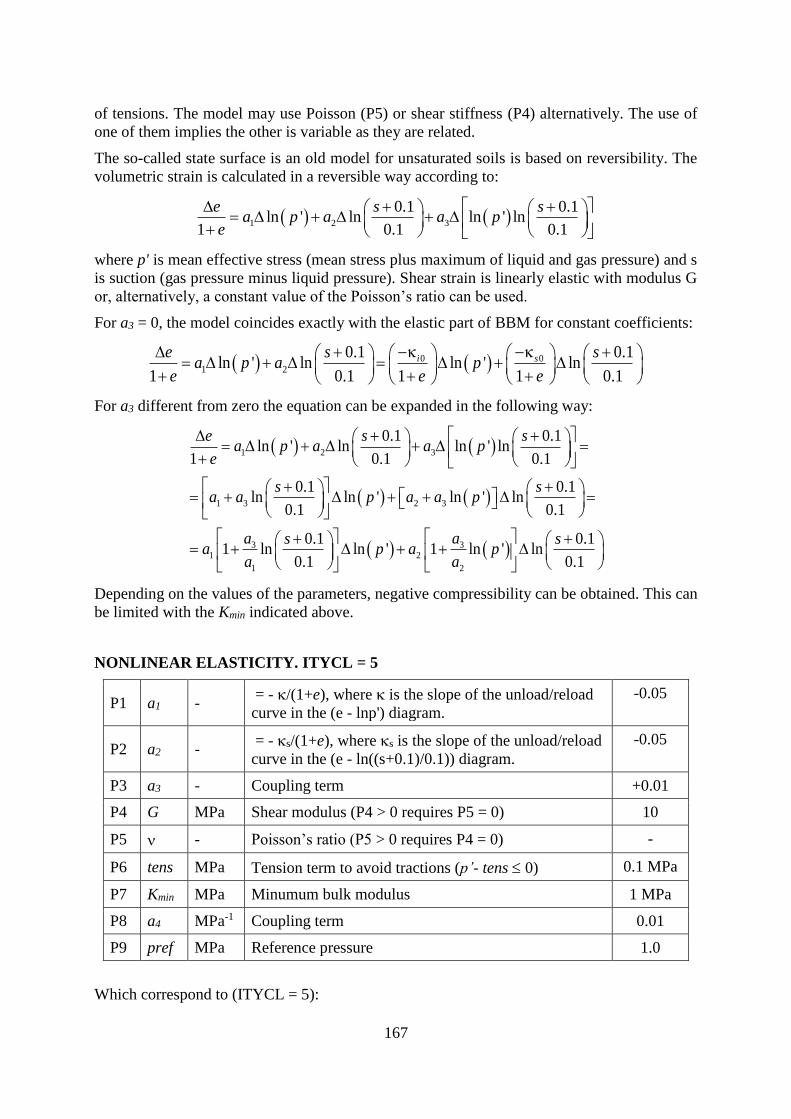
167
of tensions. The model may use Poisson (P5) or shear stiffness (P4) alternatively. The use of
one of them implies the other is variable as they are related.
The so-called state surface is an old model for unsaturated soils is based on reversibility. The
volumetric strain is calculated in a reversible way according to:
1 2 3
0.1 0.1ln ' ln ln ' ln
1 0.1 0.1
e s sa p a a p
e
where p' is mean effective stress (mean stress plus maximum of liquid and gas pressure) and s
is suction (gas pressure minus liquid pressure). Shear strain is linearly elastic with modulus G
or, alternatively, a constant value of the Poisson’s ratio can be used.
For a3 = 0, the model coincides exactly with the elastic part of BBM for constant coefficients:
0 01 2
0.1 0.1ln ' ln ln ' ln
1 0.1 1 1 0.1
i se s sa p a p
e e e
For a3 different from zero the equation can be expanded in the following way:
1 2 3
1 3 2 3
3 31 2
1 2
0.1 0.1ln ' ln ln ' ln
1 0.1 0.1
0.1 0.1ln ln ' ln ' ln
0.1 0.1
0.1 0.11 ln ln ' 1 ln ' ln
0.1 0.1
e s sa p a a p
e
s sa a p a a p
a as sa p a p
a a
Depending on the values of the parameters, negative compressibility can be obtained. This can
be limited with the Kmin indicated above.
NONLINEAR ELASTICITY. ITYCL = 5
P1 a1 - = - /(1+e), where is the slope of the unload/reload
curve in the (e - lnp') diagram.
-0.05
P2 a2 - = - s/(1+e), where s is the slope of the unload/reload
curve in the (e - ln((s+0.1)/0.1)) diagram.
-0.05
P3 a3 - Coupling term +0.01
P4 G MPa Shear modulus (P4 > 0 requires P5 = 0) 10
P5 - Poisson’s ratio (P5 > 0 requires P4 = 0) -
P6 tens MPa Tension term to avoid tractions (p’- tens 0) 0.1 MPa
P7 Kmin MPa Minumum bulk modulus 1 MPa
P8 a4 MPa-1 Coupling term 0.01
P9 pref MPa Reference pressure 1.0
Which correspond to (ITYCL = 5):

168
1 2 3 4
341 2
1 2
0.1 0.1ln ' ln ln '/ ln ln '
1 0.1 0.1
0.11 ln ' 1 ln '/ ln
0.1
ref
ref
e s sa p a a p p a s p
e
aa sa s p a p p
a a
With the following equivalence with BBM original parameters:
0 01 2 4 1 3 2
1 1
i si spa a a a a a
e e

169
VPUSR 1 (ICL = 34). ITYCL = 1
P1 1/s Fluidity 1
P2 N Power of the stress function (integer value) 5
P3 Fo MPa Fo=1 MPa 1.0
P4 exp(s)
P5 b Non associativity parameter. 0.3
VPUSR 2 (ICL = 35). ITYCL = 1
P1 n - Power in F and G (integer value) 1
P2 - Parameter in F and G -1/9 = -0.1111111
P3 s - 0 (then Fs=1, and J3D is not considered) -
P4 m - Typical value -0.5, only required if s0 -
P5 DRY - =MDRY 1.2
P6 - - -
P7 (J1o*)F MPa Positive value, initial size of F 1.2 (=3*0.4)
P8 (J1o*)G MPa Positive value, initial size of G 1.2 (=3*0.4)
P9 a - Parameter in F and G 3
P10 SAT - =MSAT 1.2
P7 and P8 describe the size of F and G. This parameter is 3 times the preconsolidation mean
stress for saturated conditions. P10 is the slope of the critical state line. This parameter can be
related to the friction angle of the material 6sin '
3 sin 'M
.
VPUSR 3 (ICL = 36). ITYCL = 1
P1 - Elastic compression parameter 0.07
P2 - Viscoplastic compression
parameter
0.19
P3 r - Parameter in LC curve 0.5
P4 - Parameter in LC curve 1
P5 pc MPa Parameter in LC curve 0.1
P6 k1 - -
P7 k2 - -0.03 = -3*0.01
P8 k3 - +0.03 = + 3*0.01
P9 k4 - 0.12 = 3*0.04
P10 - -
The viscoplastic part is independent on the elastic part. What produces irreversible
deformations is the plastic or viscoplastic part of the model. P2 is the viscoplastic compression
parameter. P3, P4 and P5 describe the LC curve.

170
CODE_BRIGHT. CONSTITUTIVE LAWS
This chapter contains the different models available and the corresponding parameters required
by each model. The following constitutive laws are available:
HYDRAULIC AND
THERMAL CONSTITUTIVE
MODELS (a)
RETENTION CURVE
INTRINSIC PERMEABILITY
LIQUID PHASE RELATIVE
PERMEABILITY
GAS PHASE RELATIVE
PERMEABILITY
DIFFUSIVE FLUXES OF MASS
DISPERSIVE FLUXES OF
MASS AND ENERGY
CONDUCTIVE FLUX OF HEAT
MECHANICAL CONSTITUTIVE MODELS
ELASTICITY (b)
NONLINEAR ELASTICITY (b)
VISCOPLASTICITY FOR SALINE MATERIALS
(b)
VISCOPLASTICITY FOR SATURATED SOILS
AND ROCKS (b)
VISCOPLASTICITY - GENERAL (b)
DAMAGE-ELASTOPLASTIC MODEL FOR
ARGILLACEOUS ROCKS (c)
THERMO-ELASTOPLASTIC MODEL FOR SOILS
(d)
BARCELONA EXPANSIVE MODEL FOR SOILS
(e)
CASM’s FAMILY MODELS (f)
PHASE PROPERTIES (a)
SOLID PHASE PROPERTIES
LIQUID PHASE PROPERTIES
GAS PHASE PROPERTIES
EXCAVATION PROCESS (g)
VI.c. DAMAGE-ELASTOPLASTIC MODEL FOR ARGILLACEOUS ROCKS
ICL NAME ITYCL DESCRIPTION
70 DAMAGE-ELASTOPLASTIC MODEL FOR ARGILLACEOUS ROCKS 1,2,3Damage orthotropic elastic model for the bonded material (1:linear damage law;
2:exponential damage law; 3:logarithmic damage law)
71 DAMAGE-ELASTOPLASTIC MODEL FOR ARGILLACEOUS ROCKS 1,2,3Linear Orthotropic elastic model parameters for the soil matrix. (1; MC; 2:HB,
3:Camclayl)
72 DAMAGE-ELASTOPLASTIC MODEL FOR ARGILLACEOUS ROCKS 1 Coupling behaviour. ITYCL = 0: bond behaviour is not activated
73 DAMAGE-ELASTOPLASTIC MODEL FOR ARGILLACEOUS ROCKS 1,2,3 MC or HB or BBM for the clay matrix - shape in p-q diagram
74 DAMAGE-ELASTOPLASTIC MODEL FOR ARGILLACEOUS ROCKS 1,2,3 MC or HB or BBM for the clay matrix - shape in deviatoric plane
75 DAMAGE-ELASTOPLASTIC MODEL FOR ARGILLACEOUS ROCKS 1,2,3 MC or HB or BBM potential for the clay matrix - shape in p-q diagram
76 DAMAGE-ELASTOPLASTIC MODEL FOR ARGILLACEOUS ROCKS 1,2,3 MC or HB or BBM plastic potential for the clay matrix - shape in the deviatoric plane
77 DAMAGE-ELASTOPLASTIC MODEL FOR ARGILLACEOUS ROCKS 1,2,3MC or HB or BBM Hardening law for clay matrix, used only if bond behaviour is not
activated
78 DAMAGE-ELASTOPLASTIC MODEL FOR ARGILLACEOUS ROCKS 1 Rate dependency parameters
79 DAMAGE-ELASTOPLASTIC MODEL FOR ARGILLACEOUS ROCKS 1 Control parameters for SPA (Backward euler scheme)
MECHANICAL CONSTITUTIVE LAWS (part c)

171
DAMAGE-ELASTOPLASTIC MODEL FOR ARGILLACEOUS ROCKS
CODES ICL = 70 to 79 ITYCL = see below
DESCRIPTION Damage-elastoplastic model for argillaceous rock This model considers
the argillaceous rock as a composite material made of a clay matrix
interlocked by bond. Clay matrix behaviour is modeled through an
elastoplastic constitutive law, typical of soils. Bonds are modeled
through a damage elastic law (Carol et al., 2001), typical of quasi-brittle
materials. A coupling parameter gives the relative importance of clay and
bond response for the composite material. This law applies to material
having a response transitional between that of a soil and a rock.
EQUATIONS
For this model, equations are written assuming Soils Mechanics
convention (p > 0, v> 0, compression). p is the mean effective stress, J
the square root of the second invariant of deviatoric stress tensor, the
Lode’ angle (-30º in triaxial compression, +30º in triaxial extension) (see
ICL 21 to 27 for their definition).
Clay matrix behaviour
Elastic law: M eM M p
ij ijkl kl kl klM
s
dsd D d d
K
M
ij are the stresses prevailing at clay particles contact, eM
ijklD is the
mechanical elastic stiffness matrix of the clay, M
kld are the strains
corresponding to the clay matrix deformation (equal to the external
strains), M
sK is the bulk modulus against suction changes (if any), p
kld
are the plastic strains of the clay matrix.
2 elastic laws are considered:
Orthotropic linear elasticity (ITYCL = 1 or 2):
eM
ijklD is defined by clay matrix Young’s moduli EMh and EM
v and
Poisson’s ratio Mh, G
Mv, M
hv and Mvh. M
sK is taken constant. Subscript
h indicate value in the direccion orthogonal to the orthotropy axis,
subscript v along the orthotropy axis (and not necessarily along the
horizontal plane and the vertical axis). The direction of orthotropy axis
is indicated for each element in the file <root>_gri.dat by the two angles
shown in the figure below.
Value of EMh is computed as:
EMh = max(EM
h0, EM
h1 pM + EM
h2)
vhere EMh0, E
Mh1 and EM
h2 are parameters of the model.

172
Camclay type orthotropic elasticity (ITYCL = 3):
eM
ijklD is defined by clay matrix bulk modulus KMh and KM
v and clay matrix
Poisson’s ratio Mh, M
v, Mhv and M
vh. Bulk modulus against stress
changes is linearly dependent of the mean stress following the
relationship:
M
M
hM
h
eK
1
M
M
vM
v
eK
1
Bulk modulus against suction changes is linearly dependent of the mean
stress following the relationship:
1 atmM
s M
s
e s pK
e is the void ratio, M and M
s the slopes of the unloading/reloading and
drying/wetting lines in the planes e-lnpM and e-ln(s + patm), respectively.
patm is the atmospheric pressure and is taken equal to 0.1 MPa.
Yield function: 3 yield criteria are considered:
Mohr-Coulomb (ITYCL = 1):
1cos sin sin ' sin '( ) 0
3
p M M M M M M
tF J p p
' cot 'M M M
tp c is clay matrix tensile strength, c’M clay matrix cohesion,
’M clay matrix friction angle.
Cohesion depends on suction following the law:
' ' 0 tanM M M
bc s c s

173
Hoek & Brown (1980) (ITYCL = 2):
2
2
4sin2 sin6
( ) 03
M
M Mp M M M M M
tM
c
mF J J m p p
R
/M M M
t cp R m is clay matrix tensile strength, RcM clay matrix uniaxial
compressive strength, mM a parameter defining the shape of the parabolic
yield criterion.
M
cR depends on suction following the law:
0 (1 )expM M M M M
c cR s R r s r
BBM model (ITYCL = 3):
2
2
0( ) 03
Mp M M M M M
t
MF J p p p p
where M
tp is the clay matrix tensile strength, 0
Mp the clay matrix
isotropic yield locus and M the slope of the critical state line in the pM –
vqM diagram. The following dependencies on suction are considered:
M M
tp k s
0
*
00 with s 0 1
M M
M MM
M sM M M M M s
c M
c
pp p r re
p
Mohr Coulomb and Hoek & Brown yield criteria present corners in the
deviatoric plane. They are smoothed using Sloan & Booker (1986)
procedure. Lode’s angle t at which smoothing starts must be defined
(see ICL = 74).
Rate dependency: Rate dependency is introduced as a visco-plastic
mechanism. Plastic multiplier p is expressed as a function of the distance
between the current clay matrix stress point and the inviscid plastic
locus:
p p
M
dtd F
where dt is the time increment, M is the clay matrix viscosity and are
the Macauley brackets. Inviscid plastic locus takes the form:
0M
p p pF F ddt
where Fp can be either the Mohr Coulomb or Hoek & Brown yield
criterion.

174
Plastic potential: A non associated plastic potential in the p-q diagram
is defined for each yield criterion. In the deviatoric plane, plastic
potential is considered associated.
Mohr-Coulomb (ITYCL = 1):
1
cos sin sin ' sin '( )3
p M M M M M M M
tG J p p
ptM, c’M and ’M are parameters defining the yield criterion. is a
parameter defining the non associativity of the flow. It takes a value equal
to 1 when associated and equal to 0 for null dilatancy.
Hoek & Brown (ITYCL = 2):
2
2
4sin2 sin6
( )3
M
M Mp M M M M M
tM
c
mG J J m p p
R
ptM, Rc
M and mM are parameters defining the yield criterion. M is a
parameter defining the non associativity of the flow. It takes a value equal
to 1 when associated and equal to 0 for null dilatancy.
Barcelona Basic Model (ITYCL = 3):
2
2
0( )3
Mp M M M M M M
t
MG J p p p p
ptM, p0
M and MM are parameters defining the yield criterion. M is a
parameter defining the non associativity of the flow. It takes a value equal
to 1 when associated and equal to 0 for null dilatancy. To respect the
condition of null lateral strain during K0–loading, M must be set to:
9 3 1
1 09 6
M M M
M
M MM
M M M
M
Hardening law:
Mohr-Coulomb (ITYCL = 1):
A softening law is introduced through the following dependency of the
tensile strength on the plastic strain:
M' cotan 'M M
tp c
with M
peak' =c'Mc if 0
pM M
eq rc
M
peakM
peak 0
0
c' 1' =c'
M
M pM M
eq rcM M
rc rc
c
if 0
M pM M
rc eq rc
M
peak' = c'M Mc if M pM
rc eq

175
and M
peak' = 'M if 0
pM M
eq r
M
peakM
peak 0
0
' 1' = '
M
M pM M
eq rM M
r r
if 0
M pM M
r eq r
M
peak' = 'M M if M pM
r eq
= c’resM / c’peak
M is a brittleness parameter for the cohesive
component,= ’resM / ’peak
M is a brittleness parameter for the
frictional component, eqpM is the equivalent plastic strain, rc0
M the
accumulated equivalent plastic strain at which the cohesion starts to
degrade, rcM the accumulated equivalent plastic strain at which the
residual cohesion cres’M is reached, r0
M the accumulated equivalent
plastic strain at which the friction angle starts to degrade, rM the
accumulated equivalent plastic strain at which the residual friction angle
’res’M is reached. = = 1 means perfect plasticity, = = 0,
total strength degradation (residual cohesion and friction angle equal to
0).
Hoek & Brown (ITYCL = 2):
A softening law is introduced through the following dependency of the
tensile strength on the plastic strain: 2
0 1max( , )1-(1 )
M pM MM Mc rt M M
r
Rp
m
Rc0M is the intact strength,a brittleness parameter, pM
1 is the major
principal plastic strain, rM the accumulated major principal plastic strain
at which the residual strength 2Rc0M is reached. is related to the
intact and residual uniaxial compressive strength Rc0M and Rcres
M by the
formula: 2
0 0
2
3
M MM Mcres cres
M M
c c
R Rm
R R
= 1 means perfect plasticity, = 0, total degradation (residual
strength equal to 0). > 1 means hardening plasticity while < 1
means softening plasticity.
Barcelona Basic Model (ITYCL = 3):
The hardening/softening law is introduced through the following
dependency of the saturated isotropic yield locus on the plastic strain: *
0
*
0
(1 )M
pM
vM M M
dp ed
p

176
Bond behaviour
Elastic law:
b eb b d
ij ijkl kl kld D d d
eb
ijklD is the secant damaged elastic matrix. It is related to the secant
undamaged elastic tensor 0eb
ijklD by 0eb L eb
ijkl ijklD e D . L is the damage
variable, related to the ratio of bond mickocraks area over the whole bond
area. 0eb
ijklD is defined by the undamaged bond Young’s modulus Eb and
bond Poisson’s ratio b through the classical linear orthotropic elasticity.
Damage locus: Damage locus is defined as an energy threshold
1( )
2
d b b b
ij ijF r s
rb is the value of energy threshold that depends on suction following:
0( )b b b
sr s r r s
0
b
sr is a parameter which controls the change of bond damage locus with
suction.
Rate dependency: Rate dependency is introduced as a delayed
microcracking and use the visco-damage formalism. Damage variable is
expressed as a function of the distance between the current bond stress
point and the infinitely slow damage locus:
d
b
dtdL F
where dt is the time increment, b is the bond viscosity and are the
Macauley brackets. Infinitly low damage locus takes the form:
0b
d dF F dLdt
Damage rule: Damage rule gives the evolution of damage strain d
kld
with damage variable L. This relation is constrained by bond elastic
moduli evolution and must take the form: d b
kl kld dL

177
Damage evolution law: It gives the evolution of damage locus rb with
damage variable L. Three different expressions may be considered:
a) linear: 0 1
b b br r r L
a) exponential: 10 exp
br Lb br r
a) logarithm: 0 1 lnb b br r r L
r0 is the damage of the intact material and r1 a parameter giving the rate
of evolution (higher value of r1 gives lower damage rate). r1 is taken
function of suction following: 1 10 1
b b b
sr r r s
10
br is a parameter which controls the damage evolution rate for the
saturated bond material and 1
b
sr is a parameter which controls the change
of damage evolution rate with suction.
Coupling behaviour: Coupling comes from the restrictions that local
strain M
ij and b
ij must be compatible with the external strain ij and local
stressesM
ij and b
ij must be in equilibrium with external stresses ij .
This restrictions read: M b
ij ij ijd d d
1 M b
ij ij ij with 2
0
Le
L is the damage variable and 0 a coupling parameter that gives the
relative importance of bond and clay matrix behaviour in the overall
response of the composite material. 00 .
Since this model requires a substantial number of parameters, several ICL's are included in
Mechanical Data 3:
Argillite Bonding (ICL = 70) contains elastic parameters for the bonding.
Argillite Matrix (ICL = 71) contains elastic parameters for the soil matrix.
Argillite – Coupling (ICL = 72) contains parameters for the coupling between bonding and
soil matrix.
Argillite – Yield vol (ICL = 73) contains parameters for the shape of the yield function in the
p-q plane (soil matrix).
Argillite – Yield dev (ICL = 74) contains parameters for the shape of the yield function in the
deviatoric plane (soil matrix).
Argillite – Plastic vol (ICL = 75) contains parameters for the shape of the plastic potential in
the p-q plane (soil matrix).
Argillite – Plastic dev (ICL = 76) contains parameters for the shape of the plastic potential in
the deviatoric plane (soil matrix).
Argillite – Hardening (ICL = 77) contains parameters for the hardening law (soil matrix).
Argillite – Visco (ICL = 78) contains parameters for the viscoplastic model (bonding and soil
matrix).
Argillite – Control parameters (ICL = 79) contains parameters to control the integration of
the constitutive law.

178
PARAMETERS FOR ARGILLITE BONDING ICL = 70 (Damage orthotropic elastic model
for the bond material). ITYCL = 1: Linear damage evolution law. ITYCL = 2: exponential
damage evolution law. ITYCL = 3: logarithm damage evolution law.
P1 Ebh MPa
Young’s modulus for the bond material in the plane
orthogonal to the direction of orthotropy
If P6 = 0 or 1 (no anisotropy), isotropic Young’s modulus
P2 bh -
Poisson’s ratio for the bond material in the plane orthogonal to
the direction of orthotropy
If P6 = 0 or 1 (no anisotropy), isotropic Poisson’s ratio
P3 rb10 MPa Damage evolution rate for the saturated bond material
P4 rb0s MPa Change of bond damage locus with suction
P5 rb1s MPa Change of bond damage evolution rate with suction
P6 Eb
h / Eb
v =
bhv / b
vh -
Ratio of anisotropy (ratio between the value of Young’s
modulus for bond material in the direction perpendicular and
parallel to the orthotropy axis)
If P6 = 0, a default value equal to 1 (no anisotropy) is assigned
to this parameters
P7 bhv - Cross Poisson’s ratio of the bond material (b
hv = dbh / db
v)
P8 Gv MPa Shear modulus of the bond material along the axis of
orthotropy (ratio dh / dv)
P9 Kbs MPa
Bulk modulus against suction changes for the bond material
(considered isotropic)

179
PARAMETERS FOR ARGILLITE MATRIX ICL = 71; ITYCL = 1 or 2 (Linear orthotropic
elastic model for the soil matrix)
P1 EMh* MPa
Young’s modulus for the saturated matrix in the plane
orthogonal to the direction of orthotropy.
If P6 = 0 or 1 (no anisotropy), isotropic Young’s modulus.
P2 Mh -
Poisson’s ratio in the plane orthogonal to the direction of
orthotropy.
If P6 = 0 or 1 (no anisotropy), isotropic Poisson’s ratio.
P3 KMs MPa Bulk modulus against suction changes (considered isotropic).
P4 EMs -
Coefficient setting the change of E with suction according to
the equation EMh = EM
h* + EMs s
P5 - - Void
P6 EM
h / EM
v =
Mhv / vh
-
Ratio of anisotropy (ratio between the value of Young’s
modulus in the direction perpendicular and parallel to the
orthotropy axis).
If P6 = 0, a default value equal to 1 (no anisotropy) is
assigned to this parameters.
P7 Mhv - Cross Poisson’s ratio (M
hv = dMh / dM
v)
P8 GMvh = GM
hv MPa Cross shear modulus (GMvh = dvh / dvh)
P9 EM1h -
Coefficient giving the change of the Young’s modulus with
the stress in the plane orthogonal to the direction of
orthotropy.
P10 EM2h MPa
Value of Young modulus in the plane orthogonal to the
direction of orthotropy at null mean (net or effective) stress.
Elastic thermal deformation will be taken into account in the model in a coupled way if the
elasticity law ICL = 5; ITYCL = 1 is used. Parameter P3 corresponds to the thermal expansion
coefficient.

180
PARAMETERS FOR ARGILLITE MATRIX ICL = 71 (Elastic model for the soil matrix);
ITYCL = 3 (Orthotropic Camclay type elastic model for the soil matrix)
P1 M Slope of the unloading-reloading line in the e –ln(h) model
If P6 = 0 or 1 (no anisotropy), Slope of the unloading-
reloading line in the e –ln(p) model.
P2 Mh -
Poisson’s ratio in the plane orthogonal to the direction of
orthotropy.
If P6 = 0 or 1 (no anisotropy), isotropic Poisson’s ratio.
P3 Ms MPa
Slope of the wetting-redrying line in the e –ln(s + patm) model
(considered isotropic).
P4 - Void
P5 - - Void
P6 KM
h / KM
v =
Mhv / vh
-
Ratio of anisotropy (ratio between the value of bulk modulus
in the direction perpendicular and parallel to the orthotropy
axis).
If P6 = 0, a default value equal to 1 (no anisotropy) is
assigned to this parameters.
P7 Mhv - Cross Poisson’s ratio (M
hv = dMh / dM
v)
P8 Gvh MPa Cross shear modulus GMvh = dvh / dvh
PARAMETERS FOR ARGILLITE – COUPLING ICL = 72; ITYCL = 1 (Coupling behaviour).
P1 0 - Coupling parameter between bond and matrix.
P2 B - Biot coefficient
P3 - - void
P4 - - void
P5 iunsat -
Flag to indicate stress concept in unsaturated conditions:
0 – Biot stress pb = p –B pl
1 – Biot/Bishop stress pb = p – [1 – Sr + B Sr] pl
P6 b -
Parameter to compute porosity as a function of damage multiplier
(d) as 0 1 expb db
This porosity is then used to compute intrinsic permeability of
Kozeny's model (ICL=7, ITYCL=1).
P7 -
Parameter to compute intrinsic permeability as a function of plastic
multiplier (p) as exp p k k
k : intrinsic permeability computed in ICL = 7
P9 bs //
C-1 Linear thermal expansion coefficient for the medium (isotropic or
parallel, positive value).
P10 bs C-1
Linear thermal expansion coefficient for the medium (perpendicular,
positive value).

181
PARAMETERS FOR ARGILLITE – COUPLING ICL = 72; ITYCL = 2 (Coupling behaviour).
P1 – P6 Same as in ICL = 72; ITYCL = 1
P7 k -
Parameter to compute intrinsic permeability as a function of plastic
multiplier (eqp
) as
3k p
0 eq1k k ε
P9 – P10 Same as in ICL = 72; ITYCL = 1
PARAMETERS FOR ARGILLITE – YIELD VOL ICL = 73; ITYCL = 1 (Mohr Coulomb
criterion for the soil matrix – shape in pM-qM diagram).
P1 ’M º Friction angle
P2 c’ M MPa Cohesion
P3 bM º
Coefficient setting the change in cohesion with suction following:
c’M = s tan(bM)
P4 M MPa-1 Coefficient setting the change in friction angle with suction.
PARAMETERS FOR ARGILLITE – YIELD VOL ICL = 73; ITYCL = 2 (Hoek & Brown
criterion for the soil matrix – shape in pM-qM diagram).
P1 m M - Ratio of uniaxial compressive strength divided by tensile strength.
P2 Rc M
MPa Uniaxial compressive strength at the reference temperature (P8
field).
P3 r M - Coefficient setting the change in cohesion with suction.
P4 M MPa-1 Coefficient setting the change in cohesion with suction.
P5 - - Void
P6 - - Void
P7 kTM
Coefficient setting the decrease of uniaxial compressive strength
with temperature.
P8 T0 Reference temperature.
PARAMETERS FOR ARGILLITE – YIELD VOL ICL = 73; ITYCL = 3 (Basic Barcelona
model criterion for the soil matrix – shape in pM-qM diagram).
P1 M M - Slope of the critical state line.
P2 - - Void
P3 r M - Coefficient setting the change in cohesion with suction.
P4 M MPa-1 Coefficient setting the change in cohesion with suction
P5 pc M MPa Reference pressure
P6 ksM - Coefficient setting the increase of tensile strength with suction.

182
PARAMETERS FOR ARGILLITE – YIELD DEV ICL = 74; ITYCL = 1, 2, 3 (Mohr Coulomb,
Hoek & Brown or Basic Barcelona model criteria for the soil matrix – shape in deviatoric
plane).
P1 t M
º Lode angle value at which corner smoothing function is tangent
to Mohr Coulomb envelope (typical value – not default – 25º).
PARAMETERS FOR ARGILLITE – PLASTIC VOL ICL = 75; ITYCL = 1, 2, 3 (Mohr
Coulomb, Hoek & Brown or Basic Barcelona model plastic potential for the soil matrix –
shape in pM-qM diagram).
P1 - Coefficient of non associativity (0: no volumetric plastic strain,
1: full volumetric plastic strain –associative plasticity).
PARAMETERS FOR ARGILLITE – PLASTIC DEV ICL = 76; ITYCL = 1, 2, 3 (Mohr
Coulomb, Hoek & Brown or Basic Barcelona model plastic potential for the soil matrix –
considered associated in the deviatoric plane).
P1 - P10 Void
PARAMETERS FOR ARGILLITE – HARDENING ICL = 77; ITYCL = 1 (Mohr Coulomb
hardening law for clay matrix).
P1 - Cohesion brittleness index: '
'
MM res
M
peak
c
c
P2 rc0M - Equivalent plastic strain at which c’M starts to degrade.
P3 rcM - Equivalent plastic strain at which c’res
M is reached.
P4 - Friction angle brittleness index: '
'
MM res
M
peak
P5 r0M - Equivalent plastic strain at which ’M starts to degrade.
P6 rM - Equivalent plastic strain at which ’res
M is reached.
PARAMETERS FOR ARGILLITE – HARDENING ICL = 77; ITYCL = 2 (Hoek & Brown
hardening law for the soil matrix).
P1 - Brittleness index: 2
0 0
2
3
M MM Mcres cres
M M
c c
R Rm
R R
P2 rM -
Brittleness interval: xir is the major compressive plastic strain
value (|1pM|) at which
M
cresR is reached.

183
PARAMETERS FOR ARGILLITE – HARDENING ICL = 77; ITYCL = 3 (Basic Barcelona
model does not need additional parameter for the hardening law for clay matrix).
P1 M(0) - Slope of the virgin loading line in the e-ln(pM) diagram.
PARAMETERS FOR ARGILLITE – HARDENING ICL = 77; ITYCL = 4 (Camclay model
plus Gallipoli et al. (2003) proposal).
P1 M(0) - Slope of the virgin loading line in the e-ln(pM) diagram.
P2 a - Parameter for the expression of the state parameter e/eSS
P3 b - Parameter for the expression of the state parameter e/eSS
P4 R - Mean pore radius
PARAMETERS FOR ARGILLITE – HARDENING ICL = 77; ITYCL = 5 (Camclay model
plus Tamagnini proposal).
P1 M(0) - Slope of the virgin loading line in the e-ln(pM) diagram.
P2 b - Parameter for the dependency of the hardening law on
the degree of saturation.
PARAMETERS FOR ARGILLITE – VISCO ICL = 78; ITYCL = 1 (Rate dependency
parameters).
P1 b MPa.s Bond viscosity
P2 MPa.s Matrix viscosity
PARAMETERS FOR ARGILLITE – CONTROL PARAMETERS ICL = 79; ITYCL = 1
(Control parameter for the Stress Point Algorithm – Backward-Euler scheme is used).
P1 tol - Tolerance over SPA residual (typical value – not default – 1.e-8)
P2 itmax - Number of SPA Newton Raphson iterations at which local
subincrementation is performed (typical value – not default – 30)
P3 isubmax - Maximum number of local (SPA) subincrementations by global
iteration (typical value – not default –500)
P4 iJac -
Flag to define the type of F.E. elementary tangent matrix to use:
1 – elastic matrix
-1 – elastoplastic tangent matrix (typical value –not default)

184
Important notes:
1. Damage only, elastoplasticity only or coupled damage-elastoplasticity can be defined
depending on the combinations of ITYCL used. They are:
ICL = 70 ICL = 71 ICL = 72 ICL = 73
Damage
only ITYCL = 1 ITYCL = 0 ITYCL = 0 ITYCL = 0
Plasticity
only ITYCL = 0 ITYCL = 1 ITYCL = 0
ITYCL = 1 for Mohr Coulomb
ITYCL = 2 for Hoek & Brown
ITYCL = 3,4,5 Basic Barcelona
model and adaptations
Coupled
damage-
elasto-
plasticity
ITYCL = 1 ITYCL = 1 ITYCL = 1
ITYCL = 1 for Mohr Coulomb
ITYCL = 2 for Hoek & Brown
ITYCL = 3 Basic Barcelona model
and adaptation
2. Inviscid damage or elastoplasticity can be defined by setting b = 0 and M = 0 (or
ITYCL = 0 for ICL = 78)
3. ITYCL for ICL = 74 to 77 are automatically set to the value of ITYCL for ICL = 73.
HISTORY VARIABLES
Argillite model requires in total 35 history variables. They are listed in the following table.
Variable 1 is the history variable of the elastoplastic model for the matrix. In the most general
case, value for this variable need to be specified in the input file (see format in the Part III).
In the case of Mohr Coulomb model (ITYCL(73) = 1), variable 1 corresponds to the tensile
strength of the material pt. If a null value is specified in the input file for this variable, the
program will compute the value of the tensile strength for each element from the cohesion and
the friction angle of the material assigned to the element. The expression used to compute the
default value is: pt = c’ cotan’.
In the case of Hoek & Brown model (ITYCL(73) = 2), variable 1 corresponds to the tensile
strength of the material pt. If a null value is specified in the input file from this variable, the
program will compute the value of the tensile strength for each element from the uniaxial
compressive strength Rc and the parameter m of the material assigned to the element. The
expression used to compute the default value is: pt = Rc / m.
In the case of Cam clay model (ITYCL(73) = 3), variable 1 corresponds to the preconsolidation
pressure of the material p0*. IF A NULL VALUE IS SPECIFIED IN THE INPUT FILE FOR
THIS VALUE, THE PROGRAM WILL ABORT DUE TO A MATH ERROR (this ellipse of
Cam clay model degenerates into a point).

185
Variable 2 is the history variable of the damage model for the bond. In the most general case,
value for this variable need to be specified in the input file (see format in the Part III). However,
in many cases, this value can be set to 0. It means that damage will start for any stress changes.
Variable 3 is used internally to keep memory of the type of constitutive matrix (elastic, tangent
elastoplastic, tangent damage or tangent damage elastoplastic) used to build the global tangent
stiffness. No input from the user is associated to this variable.
Variable 4 is the plastic multiplier of the matrix. This variable measures the amount of plastic
strain. It is usually set to 0 at the beginning of the computation and updated within the argillite
subroutine. This variable is used only by the user for output visualization purposes (it provides
the spatial distribution of plastic strain intensity within the mesh at any output time).
Variable 5 is the damage multiplier of the bonds. This variable measures the amount of
damage. It is usually set to 0 at the beginning of the computation and updated within the argillite
subroutine. This variable is used by the user for output visualization purposes only (it provides
the spatial distribution of damage intensity within the mesh at any output time).
Variables 6 to 11 are the current stresses within the bonds. Variables 12 to 17 are the stresses
within the matrix at time of bond formation. In the most general case, all these variables have
to be specified in the input file*. However, from a practical point of view, most of the problems
can be run setting these values to 0 at the beginning of the computation (in this case, the damage
locus is centered on the initial stress state at the beginning of the computation).
Variables 18 to 35 contain the total, plastic and damage strain tensor components. They are
usually set to 0 at the beginning of the computation and updated within the argillite subroutine.
These variables are used by the user for output visualization purposes only (they provides the
spatial distribution of the total, plastic and damage strain within the mesh at any output time).
Hist var Symbol Unit Description Type
1
pt
p0*
MPa
Matrix Tensile strength (Mohr Coulomb or Hoek & Brown
models, ITCL(73)=1,2). Isotropic yield point (Camclay model, ITYCL(73)=3)
Input
2 r0 MPa Bond damage locus Input
3 flag – Type of tangent matrix Internal
4 p – Plastic multiplier Output
5 d – Damage multiplier Output
6 to 11 b MPa Initial bond stress vector
(bx,
by,
bz,
bxy,
bxz,
byz)
Input
12 to 17 0 MPa Matrix stress vector at time of bond formation
(0x,
0y,
0z,
0xy,
0xz,
0yz)
Input
18 to 23 Strain vector (x, y, z, xy, xz, yz) Output
24 to 29 p Plastic strain vector (px,
py,
pz,
pxy,
pxz,
pyz) Output
30 to 35 d Damage strain vector (dx,
dy,
dz,
dxy,
dxz,
dyz) Output

186
A summary of the different options for history variables input is summarized in the following
table.
Type of
input of
history
variables
Characteristics of the problem
All variables
= 0
Mohr Coulomb
ITYCL(73) = 1
Tensile strength is
constant within each
material and
computed from
cohesion and friction
angle
Hoek & Brown
ITYCL(73) = 2
Tensile strength is
constant within each
material and computed
from uniaxial
compressive strength and
parameter m
Cam clay model
ITYCL(73) = 3
NOT POSSIBLE
Damage locus is centred on the initial stress state of the problem. Material
is not damaged at time 0 of the computation.
From t=0, damage occurs for any stress changes
Variable 1
0
Variable 2 =
0
Variable 6 to
17 = 0
Mohr Coulomb
ITYCL(73) = 1
Tensile strength can
vary from element to
element and is equal
to the specified value
for Variable 1
Hoek & Brown
ITYCL(73) = 2
Tensile strength can vary
from element to element
and is equal to the
specified value for
Variable 1
Cam clay model
ITYCL(73) = 3
Preconsolidation
pressure can vary from
element to element and
is equal to the specified
value for Variable 1
Damage locus is centred on the initial stress state of the problem. Material
is not damaged at time 0 of the computation.
Damage occurs for any stress changes
Variable 1
0
Variable 2
0
Variable 6 to
17 0
Mohr Coulomb
ITYCL(73) = 1
Tensile strength can
vary from element to
element and is equal
to the specified value
for Variable 1
Hoek & Brown
ITYCL(73) = 2
Tensile strength can vary
from element to element
and is equal to the
specified value for
Variable 1
Cam clay model
ITYCL(73) = 3
Preconsolidation
pressure can vary from
element to element and
is equal to the specified
value for Variable 1
Damage locus is centred on the stress state at time of bond stress state of
the problem. It reflects the history of damage previous to time 0 of the
computations.
Damage occurs only when the energy input to the material is equal to the
specified value for Variable 2
Variables 3, 4 and 18 to 35 can be specified in the input file when the history of plastic and
damage strain previous to the current computations is wanted to be reproduced (particularly in
case of restart).

187
CODE_BRIGHT. CONSTITUTIVE LAWS
This chapter contains the different models available and the corresponding parameters required
by each model. The following constitutive laws are available:
HYDRAULIC AND
THERMAL CONSTITUTIVE
MODELS (a)
RETENTION CURVE
INTRINSIC PERMEABILITY
LIQUID PHASE RELATIVE
PERMEABILITY
GAS PHASE RELATIVE
PERMEABILITY
DIFFUSIVE FLUXES OF MASS
DISPERSIVE FLUXES OF
MASS AND ENERGY
CONDUCTIVE FLUX OF HEAT
MECHANICAL CONSTITUTIVE MODELS
ELASTICITY (b)
NONLINEAR ELASTICITY (b)
VISCOPLASTICITY FOR SALINE MATERIALS
(b)
VISCOPLASTICITY FOR SATURATED SOILS
AND ROCKS (b)
VISCOPLASTICITY - GENERAL (b)
DAMAGE-ELASTOPLASTIC MODEL FOR
ARGILLACEOUS ROCKS (c)
THERMO-ELASTOPLASTIC MODEL FOR SOILS
(d)
BARCELONA EXPANSIVE MODEL FOR SOILS
(e)
CASM’s FAMILY MODELS (f)
PHASE PROPERTIES (a)
SOLID PHASE PROPERTIES
LIQUID PHASE PROPERTIES
GAS PHASE PROPERTIES
EXCAVATION PROCESS (g)
VI.d. THERMO-ELASTOPLASTIC MODEL
ICL NAME ITYCL DESCRIPTION
21 THERMOELASTOPLASTIC MODEL FOR UNSATURATED SOILS 1 Contain elastic parameters
22 THERMOELASTOPLASTIC MODEL FOR UNSATURATED SOILS 1 Contain parameters for the thermal terms
23 THERMOELASTOPLASTIC MODEL FOR UNSATURATED SOILS 1 Contain plastic parameters
24 THERMOELASTOPLASTIC MODEL FOR UNSATURATED SOILS 1 Contain plastic parameters (2)
25 THERMOELASTOPLASTIC MODEL FOR UNSATURATED SOILS 1,2,3Contain parameters for the function gy (Mohr-Coulomb function, van Eeckelen function,
Von mises)
26 THERMOELASTOPLASTIC MODEL FOR UNSATURATED SOILS 1,2,3Contain parameters for the function gp (Mohr-Coulomb function, van Eeckelen function,
Von mises)
27 THERMOELASTOPLASTIC MODEL FOR UNSATURATED SOILS 1 Contain parameters for the integration of the model
MECHANICAL CONSTITUTIVE LAWS (part d)
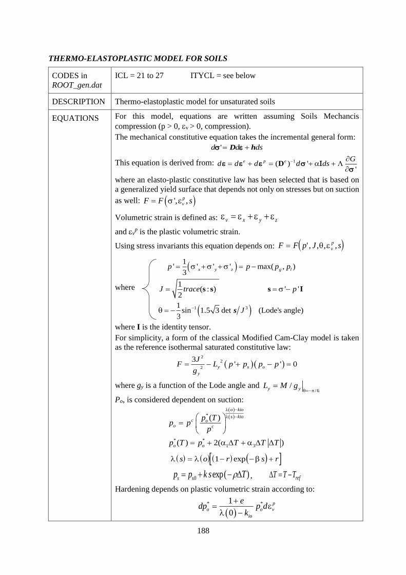
188
THERMO-ELASTOPLASTIC MODEL FOR SOILS
CODES in
ROOT_gen.dat
ICL = 21 to 27 ITYCL = see below
DESCRIPTION Thermo-elastoplastic model for unsaturated soils
EQUATIONS
For this model, equations are written assuming Soils Mechancis
compression (p > 0, v > 0, compression).
The mechanical constitutive equation takes the incremental general form:
d d ds ' D h
This equation is derived from: 1( ) ''
e p e Gd d d d ds
D
where an elasto-plastic constitutive law has been selected that is based on
a generalized yield surface that depends not only on stresses but on suction
as well: ', ,p
vF F s
Volumetric strain is defined as: v x y z
and vp is the plastic volumetric strain.
Using stress invariants this equation depends on: F F p J sv
p ' , , , ,
where
1 3
1' ' ' ' max( , )
3
1( : ) ' '
2
1sin 1.5 3 det (Lode's angle)
3
x y z g lp p p p
J trace p
J
s s s I
s
where I is the identity tensor.
For simplicity, a form of the classical Modified Cam-Clay model is taken
as the reference isothermal saturated constitutive law:
2
2
2
3' ' 0y s o
y
JF L p p p p
g
where gy is a function of the Lode angle and / 6
/y yL M g
Po, is considered dependent on suction:
*
* *
1 3
( )
( ) 2( )
o kio
s kioc o
o c
o o
p Tp p
p
p T p T T T
s o r s r 1 exp
0 exp( )s sp p k s T , refTTT
Hardening depends on plastic volumetric strain according to:
* *1
0
p
o o v
io
edp p d
k

189
Since this model requires a substantial number of parameters, several ICL's are included:
TEP – Elastic parameters (ICL = 21) contains elastic parameters (ITYCL = 1).
TEP – Thermal and other parameters (ICL = 22) contains other parameters (ITYCL = 1).
TEP – Plastic parameters 1 (ICL = 23) contains plastic parameters (ITYCL = 1).
TEP – Plastic parameters 2 (ICL = 24) contains parameters for different aspects (ITYCL = 1).
TEP – Parameters Shape Yield Surf. (ICL = 25) contains parameters for the function gy (ITYCL
= 1, 2, 3).
TEP – Parameters Shape Plastic Pot. (ICL = 26) contains parameters for the function gp (ITYCL
= 1, 2, 3).
TEP – Integration Control Parameters (ICL = 27) contains parameters for the integration of the
model (ITYCL = 1).
EQUATIONS
(continuation)
The plastic potential is taken as:
2
2
2
3' 'p s o
p
JG L p p p p
g
where gp is a function of the Lode angle and
/ 6/p pL M g
is a non-asociativity parameter.
The variation of stress-stiffness with suction and, especially, the variation
of swelling potential with stress and suction have been considered. Elastic
component of the model (volumetric strains):
dk s
e
dp
p
k p s
e
ds
sT dTv
e i s
o
( ) '
'
( ' , )
.( )
1 1 012 2
where: 0.1
( ) 1 ln0.1
i io i il
sk s k s
( ', ) 1 ln ' exps so sp ref ssk p s k p p s
For deviatoric elastic strains, a constant Poisson’s ratio is used.
Strain-dependent shear modulus model (for small strains)
Evolution of the small-strain shear stiffness G with shear strain:
G
G
a
0
0.7
1
n
ref pG G
0 0
0.1
Where refG0 is the initial shear modulus at a reference mean stress (p) of
0.1 MPa (default = 0), is the invariant of the deviatoric strain tensor and
0.7 is the shear strain at which the modulus G is 0.722·G0 (approximately
0.7·G0).
In order to “activate” this model, then refG0 (ICL=22; ITYCL=1; P7) and
0.7 (ICL=22; ITYCL=1; P8) must be greater than 0.

190
PARAMETERS FOR ICL = 21 (TEP Elastic Parameters); ITYCL = 1
P1 io - Initial (zero suction) elastic slope for specific volume-mean stress.
P2 so - Initial (zero suction) elastic slope for specific volume-suction.
P3 Kmin MPa Minimum bulk module.
P4 - -
P5 - Poisson’s ratio (-1 < < 0.5).
P6 ss - Parameter for s (only for expansive material).
P7 il - Parameter for i (only for expansive material).
P8 i - Parameter for i (only for expansive material).
P9 sp - Parameter for s (only for expansive material).
P10 pref MPa Reference mean stress (only for expansive material).
PARAMETERS FOR ICL = 22 (TEP Thermal and Other Parameters); ITYCL = 1
P1 o C-1 Parameter for elastic thermal strain
P2 1 MPa C-1 Parameter for plastic thermal strain
P3 2 C-2 Parameter for elastic thermal strain
P4 3 MPa C-2 Parameter for plastic thermal strain
P5 Tref C Reference temperature
P6 b - Biot coefficient (default value = 1)
P7 refG0 MPa Initial shear modulus at a reference mean stress (p) of 0.1 MPa
(default = 0).
If P7 = 0 => G obtained from bulk modulus and Poisson’s ratio.
If P8 = 0 =>refG G 0 (default = 0).
If P8 > 0 => Strain-dependent shear modulus model is used.
P8 0.7 - Shear strain at which the modulus G is 0.722·G0
P9 a - Parameter (default value = 0.385)
P10 n - Parameter (default value = 0.2)
PARAMETERS FOR ICL = 23 (TEP Plastic Parameters 1); ITYCL = 1
P1 (0) Slope of void ratio - mean stress curve at zero suction
P2 r Parameter defining the maximum soil stiffness
P3 MPa-1 Parameter controlling the rate of increase of soil stiffness with suction
P4 C-1 Parameter that takes into account decrease of tensile strength due to
temperature
P5 k Parameter that takes into account increase of tensile strength due to suction
P6 ps0 MPa Tensile strength in saturated conditions

191
PARAMETERS FOR ICL = 24 (TEP Plastic Parameters 2); ITYCL = 1
P1 pc MPa Reference pressure
P2 M Critical state line parameter
P3 Non-associativity parameter
P4 eo Initial void ratio
P5 po* MPa Initial preconsolidation mean stress for saturated soil
PARAMETERS FOR ICL = 25 (TEP Parameters Shape Yield Surf.); ITYCL = 1
Mohr Coulomb function: gy () = sin / (cos+ 0.577sin sin)
P1 deg
PARAMETERS FOR ICL = 25 (TEP Parameters Shape Yield Surf.); ITYCL = 2
van Eeckelen function: gy () = X/Y sin3-Z
P1 X
P2 Y
P3 Z
PARAMETERS FOR ICL = 25 (TEP Parameters Shape Yield Surf.); ITYCL = 3
Von Mises (default option): gy () = 1
PARAMETERS FOR ICL = 26 (TEP Parameters Shape Plastic Pot.); ITYCL = 1
Mohr Coulomb function: gp () = sin / (cos + 0.577sin sin)
P1 deg
PARAMETERS FOR ICL = 26 (TEP Parameters Shape Plastic Pot.); ITYCL = 2
van Eeckelen function: gp () = X/Y sin3-Z
P1 X
P2 Y
P3 Z
PARAMETERS FOR ICL = 26 (TEP Parameters Shape Plastic Pot.); ITYCL = 3
Von Mises (default option): gp () = 1

192
PARAMETERS FOR ICL = 27 (TEP Integration Control Parameters); ITYCL = 1
P1 Tole1 Yield surface tolerance (typically 1.e-8).
P2 Tole2 Elastic integration tolerance (typically between 1.e-4 and 1.e-6).
P3 Tole3 Plastic integration tolerance (typically between 1.e-4 and 1.e-2).
P4 Integration weight (ranges from 0 to 1) (typically 1).
P5 Index -1 elastoplastic matrix (typical value).
+1 elastic matrix.
P6 Itermaxc Maximum allowed subincrementations. When this value is reached, the
execution continues even if stress errors are large. Default=100.
Note that if Itermaxc > Itermaxs this condition is not used.
P7 Itermaxs Maximum allowed subincrementations. When this value is reached, the
stress and stiffness matrices calculation stops and the time step is reduced.
A message about the type of problem encountered appears. Default=10.
P10 Index2 Indicator of stress option: (0: net stress; 1: Bishop’s stress)
The integration procedure is based on an incremental scheme. A second-order integration
procedure is used in order to obtain an integration error estimation. is considered as a weight
in the evaluation of second-order integration matrix and vectors.
HISTORY VARIABLES:
The Thermo-elastoplastic (ICL = 21 to 27) model requires two history variables:
Hist_var 1 Po* MPa Evolution of preconsolidation mean stress for saturated soil
Hist_var 2 eo Evolution of void ratio
These variables can be assigned as initial conditions on surfaces/volumes if an initial particular
distribution on the geometry is required. The procedure is the same as followed by initial
stresses as was described in chapter II. PREPROCESS, PROBLEM DATA, section II.2.3.5.
If no value is assigned for these variables in conditions, internally, the program sets the input
parameters P4 (for e0) and P5 (for Po*) of the ICL=24, as initial values.
The evolution of Po* can be visualized as an output in Post-process GID interface.
Note: Effective stresses plotted in the Post-process GID interface correspond with net stresses
for unsaturated conditions and Terzaghi's effective stresses for saturated conditions. Stress and
strain invariants follow the soil mechanics notation (positive for compression).
______

193
CODE_BRIGHT. CONSTITUTIVE LAWS
This chapter contains the different models available and the corresponding parameters required
by each model. The following constitutive laws are available:
HYDRAULIC AND
THERMAL CONSTITUTIVE
MODELS (a)
RETENTION CURVE
INTRINSIC PERMEABILITY
LIQUID PHASE RELATIVE
PERMEABILITY
GAS PHASE RELATIVE
PERMEABILITY
DIFFUSIVE FLUXES OF
MASS
DISPERSIVE FLUXES OF
MASS AND ENERGY
CONDUCTIVE FLUX OF
HEAT
MECHANICAL CONSTITUTIVE MODELS
ELASTICITY (b)
NONLINEAR ELASTICITY (b)
VISCOPLASTICITY FOR SALINE MATERIALS (b)
VISCOPLASTICITY FOR SATURATED SOILS AND
ROCKS (b)
VISCOPLASTICITY - GENERAL (b)
DAMAGE-ELASTOPLASTIC MODEL FOR
ARGILLACEOUS ROCKS (c)
THERMO-ELASTOPLASTIC MODEL FOR SOILS
(d)
BARCELONA EXPANSIVE MODEL FOR SOILS (e)
CASM’s FAMILY MODELS (f)
PHASE PROPERTIES (a)
SOLID PHASE PROPERTIES
LIQUID PHASE PROPERTIES
GAS PHASE PROPERTIES
EXCAVATION PROCESS (g)
VI.e. BARCELONA EXPANSIVE MODEL
MECHANICAL CONSTITUTIVE LAWS (part e) – Mechanical data 4
ICL NAME ITYCL DESCRIPTION
80 Barcelona Expansive Model BExM - Inactive
1 Inactive
81 Barcelona Expansive Model BExM - Elastic
1 Elastic model
82 Barcelona Expansive Model BExM - Coupling
1 Coupling behavior – Interaction functions
83 Barcelona Expansive Model BExM - Yield surface
1 BBM – shape in p-q diagram
84 Barcelona Expansive Model BExM - Inactive2
1 Inactive
85 Barcelona Expansive Model BExM - Plastic potential
1 BBM plastic potential – shape in p-q diagram
86 Barcelona Expansive Model BExM - Inactive3
1 Inactive
87 Barcelona Expansive Model BExM - Hardening
1 BBM Hardening law
88 Barcelona Expansive Model BExM - Convergence
1 Control parameters for the integration of the model

194
BARCELONA EXPANSIVE MODEL FOR SOILS (BExM)
CODES ICL = 80 to 88 (Mechanical data 4) ITYCL = 1
DESCRIPTION Elastoplastic constitutive law for expansive soils (BExM by Alonso et al.,
1999).
EQUATIONS
For this model, equations are written assuming Soils Mechanics convention
(p > 0, v> 0, compression). p is the mean effective stress, J the square root
of the second invariant of deviatoric stress tensor, the Lode’ angle (-30º
in triaxial compression, +30º in triaxial extension) (see ICL 21 to 27 for
their definition).
Two levels of soil structure are defined: macrostructural level (Macro) and
microstructural level (micro) (see Appendix at the end of section VIe):
where:
Total volume
Volume of macropores
Volume of micropores
Total volume of pores (= )
Volume of solid particles
Volume of aggregates (= )
T
M
p
m
p
M m
p p p
s
m
ag s p
V
V
V
V V V
V
V V V
Micropores are assumed saturated.
The following definitions are stablished:
Total porosity over total volume:p
T
Vn
V
Macro porosity over total volume:
M
pM
T
Vn
V
Micro porosity over total volume:
m
pm
T
Vn
V
Micro porosity over volume of aggregates: m m
p pm
m
ag s p
V Vn
V V V
VT
Vs
Vpm
VpM Vp
M
Vs
Vp
Vag

195
Total void ratio: p
s
Ve
V
Macro void ratio: M
pM
ag
Ve
V
Micro void ratio:
m
pm
s
Ve
V
These definitions lead to the following relationships:
1
1
1
MM
M
mm
m
ne
n
ne
n
ne
n
1
1
1
MM
M
mm
m
en
e
en
e
en
e
1m M me e e e M mn n n
1m m Mn n n 1M m Mn n n n
The following additive equation for the total strain rate holds: Macro micro
kl kl kld d d
where
kld is the total strain rate: 1
kl
detr
e
;
Macro
kld is the macrostructural strain rate, associated to the
macroskeleton: 1
MMacro
kl M
detr
e
;
micro
kld is the microstructural strain rate (only volumetric behaviour is
considered at this level): 1
mMicro
kl m
detr
e
Elastic law:
3
3
MacroMacro Macro LC SD SI
ij ijkl kl kl kl kl klMacro
s
micromicro micro
ij ijkl kl kl micro
s
dsd D d d d d
K
dsd D d
K
Macro
ijklD is the mechanical elastic stiffness matrix which relates stress and
elastic deformation at macro level ( Macro
kld );
micro
ijklD is the mechanical elastic stiffness which relates stress and elastic
deformation at micro level ( micro
kld ).
Macro
sK is the bulk modulus against macro suction changes and micro
sK the
bulk modulus against micro suction changes. LC
kld are the macro plastic strains if LC is activated.
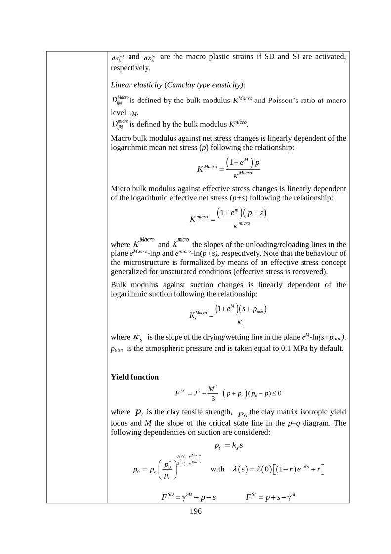
196
SD
kld and SI
kld are the macro plastic strains if SD and SI are activated,
respectively.
Linear elasticity (Camclay type elasticity):
Macro
ijklD is defined by the bulk modulus KMacro and Poisson’s ratio at macro
level M. micro
ijklD is defined by the bulk modulus Kmicro.
Macro bulk modulus against net stress changes is linearly dependent of the
logarithmic mean net stress (p) following the relationship:
1 M
Macro
Macro
e pK
Micro bulk modulus against effective stress changes is linearly dependent
of the logarithmic effective net stress (p+s) following the relationship:
1 m
micro
micro
e p sK
where Macro and
micro the slopes of the unloading/reloading lines in the
plane eMacro-lnp and emicro-ln(p+s), respectively. Note that the behaviour of
the microstructure is formalized by means of an effective stress concept
generalized for unsaturated conditions (effective stress is recovered).
Bulk modulus against suction changes is linearly dependent of the
logarithmic suction following the relationship:
1 M
atmMacro
s
s
e s pK
where s is the slope of the drying/wetting line in the plane eM-ln(s+patm).
patm is the atmospheric pressure and is taken equal to 0.1 MPa by default.
Yield function
2
2
0( ) 03
LC
t
MF J p p p p
where tp is the clay tensile strength, 0p the clay matrix isotropic yield
locus and M the slope of the critical state line in the p–q diagram. The
following dependencies on suction are considered:
t sp k s
0
*
00 with s 0 1
Macro
Macross
c
c
pp p r e r
p
SD SDF p s
SI SIF p s

197
Rate dependency
Rate dependency is introduced as a visco-plastic mechanism. Plastic
multiplier p is expressed as a function of the distance between the current
stress point and the inviscid plastic locus:
p dtd F
where dt is the time increment, is the clay viscosity and are the
Macauley brackets. Inviscid plastic locus takes the form:
0pF F ddt
where F can be either the LC, SD or SI yield criterion
Plastic potential
2
2
0( )3
p
t
MG J p p p p
0,tp p and M are parameters defining the yield criterion. is a parameter
defining the non associativity of the flow. It takes a value equal to 1 when
associated and equal to 0 for null dilatancy. To respect the condition of null
lateral strain during K0–loading, must be set to:
9 3 1
9 6 1 0
M M M
M
In the deviatoric plane, plastic potentials are considered associated.
An associated plastic potential in the p - q diagram is defined for SD and
SI.
Hardening law:
The hardening/softening law is introduced through the following
dependency of the saturated isotropic yield locus on the plastic strain:
*
0
*
0
(1 ) LC SD SI
vol vol vol
dp ed d d
p
micro microSD SD SI
vol volSD SI
K Kd d d
f f
micro microSI SD SI
vol volSD SI
K Kd d d
f f
where SDf and
SIf are the micro-macro interaction functions defined as
follow:
0 1
0
1
SDn
SD
SD SD
pf f f
p
and 0 1
0
SIn
SI
SI SI
pf f f
p

198
Model parameters should be introduced in the following ICL:
BExM – Inactive (ICL = 80) VOID
BExM – Elastic (ICL = 81) contains parameters of elastic model
BExM – Coupling (ICL = 82) contains parameters of coupling
BExM – Yield surface (ICL = 83) contains parameters for the shape of the yield function
in the p-q plane
BExM – Inactive2 (ICL = 84) VOID
BExM – Plastic potential (ICL = 85) contains parameters for the shape of the plastic
potential in the p-q plane
BExM – Inactive3 (ICL = 86) VOID
BExM – Hardening (ICL = 87) contains parameters for the hardening law
BExM – Convergence (ICL = 88) contains parameters to control the integration of the
constitutive law
PARAMETERS FOR BEXM – INACTIVE ICL = 80; ITYCL = 1 (INACTIVE)
PARAMETERS FOR BEXM – ELASTIC ICL = 81; ITYCL = 1 (Elastic model)
P1 Macro - Matrix elastic stiffness parameter at macro level for changes in
mean stress ( p )
P2 micro - Matrix elastic stiffness parameter at micro level for changes in
mean effective stress ( microp s )
P3 void -
P4 void -
P5 s -
Elastic macro stiffness parameter for changes in macro suction
( Macros )
P6 M - Poisson’s ratio
P7 min
MacroK MPa Minimum bulk modulus at macro level
P8 min
microK MPa Minimum bulk modulus at micro level
P10 If P10 ≠ 0 ⇒ total porosity is used instead of macroporosity
PARAMETERS FOR BEXM – COUPLING ICL = 82; ITYCL = 1 (Coupling behaviour).
P1 void -
P2 void -
P3 0sdf - Parameter micro-macro coupling functions when SD is active
P4 1sdf - Parameter micro-macro coupling functions when SD is active
P5 sdn - Parameter micro-macro coupling functions when SD is active
P6 0sif - Parameter micro-macro coupling functions when SI is active
P7 1sif - Parameter micro-macro coupling functions when SI is active

199
P8 sin - Parameter micro-macro coupling functions when SI is active
PARAMETERS FOR BEXM – YIELD SURFACE ICL = 83; ITYCL = 1 (Basic Barcelona
model criterion for the clay – shape in p-q diagram).
P1 M - Slope of the critical state line
P2 void - -
P3 r - Coefficient setting the change in cohesion with suction
P4 MPa-1 Coefficient setting the change in cohesion with suction
P5 pc MPa Reference pressure
P6 ks - Coefficient setting the increase of tensile strength with
suction
P7 0tp MPa Cohesion corresponding to suction equal to zero
PARAMETERS FOR BEXM – INACTIVE2 ICL = 84; ITYCL = 1 (INACTIVE)
PARAMETERS FOR BEXM – PLASTIC POTENTIAL ICL = 85; ITYCL = 1 (Basic
Barcelona model plastic potential for the clay– shape in p-q diagram).
P1 - Coefficient of non associativity (0: no volumetric plastic
strain, 1: full volumetric plastic strain –associative plasticity)
PARAMETERS FOR BEXM – INACTIVE3 ICL = 86; ITYCL = 1 (INACTIVE)
PARAMETERS FOR BEXM – HARDENING ICL = 87; ITYCL = 1 (Basic Barcelona model
does not need additional parameter for the hardening law for clay).
P1 (0) - Slope of the virgin loading line in the e-ln(p) diagram
P2 MPa.s Clay viscosity parameter
PARAMETERS FOR BEXM – CONVERGENCE ICL = 88; ITYCL = 1 (Control parameter
for the Stress Point Algorithm – Backward-Euler scheme is used).
P1 tol - Tolerance over SPA residual
(typical value – not default – 1.e-8)
P2 tol_for_subin - Tolerance over the elastic subincrementation
(typical value 1e-4)
P3 void -
P4 toler_ini_SI_SD MPa Initial separation between SI and SD
(typical value 1.e-4)

200
HISTORY VARIABLES:
The Barcelona Expansive Model (BExM) (ICL = 80 to 88) model requires the following
history variables:
Hist_var 1 P0* MPa Initial preconsolidation mean stress for saturated soil
Hist_var 2 SD MPa Initial value of the parameter that defines the position
of SD yield surface
Hist_var 3 SI MPa Initial value of the parameter that defines the position
of SI yield surface
Hist_var 4 nm Initial microstructural porosity
(micropore volume Vpm / total volume VT)
These variables can be assigned as initial conditions on surfaces/volumes if an initial particular
distribution on the geometry is required. The procedure is the same as followed by initial
stresses as was described in chapter II. PREPROCESS, PROBLEM DATA, section II.2.3.5.
Initial values of P0* defining the initial position of LC surface are required.
By default, initial position of the surfaces SD and SI is fixed using the initial stress state
involving no elastic region between SD and SI surface. To do this, first SI is computed as SI =
p+smicro, then, the position of SD is computed using an initial separation between SI and SD
surfaces which is prescribed as an input parameter in P4 of the ICL=88. If user wants to control
the initial position of SD and SI, then, specific values should be introduced as initial conditions
on surfaces/volumes, otherwise, these values should be keep as zero.
The evolution of history variables can be visualized as an output in Post-process GID interface.
Note: Effective stresses plotted in the Post-process GID interface correspond with net stresses
for unsaturated conditions and Terzaghi's effective stresses for saturated conditions. Stress and
strain invariants follow the soil mechanics notation (positive for compression).

201
APPENDIX: ABOUT THE NOTIONS OF MICRO- AND MACRO-STRUCTURES IN
THE DOUBLE-STRUCTURE MODEL IMPLEMENTED IN CODE_BRIGHT
The double structure models have been historically developed in order to reproduce the
behavior of unsaturated expansive clays (Gens & Alonso, 1992; Alonso et al., 1999). In this
seminal model, two levels of structure are considered (see Figure ):
1. The microstructure, corresponding to the clay particles made of active minerals take place. As such, the microstructure is provided with a reversible strain-stress relationship derived from considerations about double-layer theory:
dϵv = 𝛽𝑚𝑒𝛼𝑚𝑝𝑑𝑝
2. Macrostructure: Responsible of the structural rearrangements. At this level the response of collapse and loading occur. The relation of stress and strains is defined by the BBM model (Alonso et al. 1990).
Figure VIe.1. Structural levels considered (Sánchez et al. 2005)
A clear picture of what is the micro and macro-structure can be illustrated by looking at the
pore size distribution obtained in FEBEX bentonite (Figure VIe.2). Macropores corresponds in
this case to voids with entrance radii close to 30 m while the microstructure has radii around
70 Å.
Even so, this model does not refer to unique process, or size of pores. The model is able to
reproduce other types of problems. The mathematical formulation for double structure soils
presented by Sánchez et al. 2005, is referred to the FEBEX bentonite, which present a clear
double structure evidenced by the pore size distribution test presented in Figure VIe.2.
Formulation can be also used to model types of materials, provided two main pores families
can be observed in the pore size distribution curve. An example is for example provided by
the work on compacted silty clay. In this case, the macrostructure refers to the arrangement of
silt particles and the large pores between them with entrance radii of order of 10 m. The
microstructure refers to the clay particles and with entrance radii close to 1 mm.

202
Figure VIe.2 Pore Size Distribution of FEBEX Bentonite (Sánchez et al. 2005)
Figure VIe.3 Pore Size Distribution of compacted Jossigny silt (Casini et al. 2012)
Double-structure model can be used in this case to reproduce the fact that the stress dependency
of microstructure is much lower than that of macrostructure. In this case, as the scale of the
microstructure corresponds to the size of clay particles, the phenomenological law considered
is taken from classical expression for soils:
dϵv =(1 + 𝑒𝑚)𝑑𝑝
𝜅𝑚
Model can be also used to model three-level structures materials as, for example, a mixture of
bentonite powder with high density bentonite pellets. Three main pore families have been
detected in these types of materials, as shown in Figure VIe.4.

203
Figure VIe.4. Pore Size Distribution of mixture Bentonite powder/high density bentonite
pellets (Alonso et al., 2011)
In this case, the use of the double structure model needs an arbitrary split of the pore size
distribution into two pore family, according to the requirements of the modelling
(compressibility, permeability changes, …).
As a conclusion, concepts of micro and macro-structure define essentially two different levels
of scale within the material, not related to absolute value of pore size. For this reason, this type
of models can also be used to model fissured materials when the upper scale corresponds to
fissures and the lower scale to matrix.

204
CODE_BRIGHT. CONSTITUTIVE LAWS
This chapter contains the different models available and the corresponding parameters required
by each model. The following constitutive laws are available:
HYDRAULIC AND
THERMAL CONSTITUTIVE
MODELS (a)
RETENTION CURVE
INTRINSIC PERMEABILITY
LIQUID PHASE RELATIVE
PERMEABILITY
GAS PHASE RELATIVE
PERMEABILITY
DIFFUSIVE FLUXES OF MASS
DISPERSIVE FLUXES OF
MASS AND ENERGY
CONDUCTIVE FLUX OF HEAT
MECHANICAL CONSTITUTIVE MODELS
ELASTICITY (b)
NONLINEAR ELASTICITY (b)
VISCOPLASTICITY FOR SALINE MATERIALS
(b)
VISCOPLASTICITY FOR SATURATED SOILS
AND ROCKS (b)
VISCOPLASTICITY - GENERAL (b)
DAMAGE-ELASTOPLASTIC MODEL FOR
ARGILLACEOUS ROCKS (c)
THERMO-ELASTOPLASTIC MODEL FOR SOILS
(d)
BARCELONA EXPANSIVE MODEL FOR SOILS
(e)
CASM’s FAMILY MODELS (f)
PHASE PROPERTIES (a)
SOLID PHASE PROPERTIES
LIQUID PHASE PROPERTIES
GAS PHASE PROPERTIES
EXCAVATION PROCESS (g)
VI.f. CASM’s FAMILY MODELS
ICL NAME ITYCL DESCRIPTION
90 Clay and Sand model (CASM): GENERAL 1 Contain general parameters for CASM (saturated)
91 Clay and Sand model (CASM):SPECIFIC 2 Contain parameters for Unsaturated CASM model
3 Contain parameters for Cemented CASM model
4 Contain parameters for Doble hardening CASM model
MECHANICAL CONSTITUTIVE LAWS (part f)

205
CASM's FAMILY MODELS
CODES in
ROOT_gen.dat
ICL = 90, 91 (Mechanical data 3) ITYCL = 1, 2 ,3, 4
DESCRIPTION Clay and Sand model for soils (CASM)
EQUATIONS ICL = 90 (CASM – General); ITYCL = 1: Saturated CASM model
Yield function:
The yield function for CASM (Yu, 1998) expressed for a general stress state
is:
n
J pf
M p r P
'
0
3 1 'ln
' ln
where: p’ is the mean effective stress
ij ijJ trace p
1/ 21
'2
(for axi-symmetric conditions: 3q J )
P '
0 is the preconsolidation pressure
M is the slope of the critical state line
n is a constant used to specify the shape of the yield surface
r is a spacing ratio introduced to control the location of the intersection of
the critical state line with the yield surface.
M , is expressed as a function of Lode’s angle , and determines the shape
of the failure surface in the deviatoric plane. The relationship proposed by
Sheng et al (2000), to approximate a hexagonal Mohr-Coulomb failure
surface is adopted:
M M
1/44
4 4
2
1 (1 )sin3
where M is the slope of the CSL under triaxial compression ( 30º ). The
parameter controls the difference of the strengths between the triaxial
compression and extension. Often, is taken as: cs
cs
3 sin
3 sin where
cs denotes the friction angle of the soil at the critical state.

206
EQUATIONS ICL = 90 (CASM – General); ITYCL = 1: Saturated CASM model
(continued)
Hardening parameter:
Similar to the Cam-clay models, in CASM the change in size of the yield
surface dP'
0( ) is assumed to be related to the incremental plastic
volumetric by:
PdP d
'
' p0
0 v* *
where: e
*
01
and e
*
01
are the modified compression index
and modified elastic swelling index.
Plastic potential:
The plastic potential for CASM follows the stress-dilatancy relation of
Rowe (1962).
p J J
g M M Mp p
' 2 3 33 ln 3 2 ln 3 3 ln 3
' '
Where is a size parameter, which can be determinate easily for any given
stress state (p’,J) by solving the above equation and it is internally
computed.
Elastic behaviour:
The elastic behaviour of this critical state model is the same as in the Cam
–clay models with the tangent modulus (K) and shear modulus (G) being
defined by the following expressions (a constant Poisson’s ratio () is
assumed):
pK
*
'
3 1 2
2 1
KG
Undrained analysis in terms of the undrained shear strenght parameter
(Su) (Optional case):
When this option is activated, the desired undrained shear strength Su of the
material will be fitted and is not more a result of the constitutive model. To
do this, the spacing ratio r is calculated as a function of the undrained shear
strength Su (which is a input parameter in this case) to obtain a yield surface
shape that will result in the desired Su , as,
e
u
M Pr
S
1'cos
3e
o
pP p
P
'
'
''
This expression links a total stress characteristic of the soils, the undrained
shear strength, with effective stress parameters and the consolidation history
of the soil.
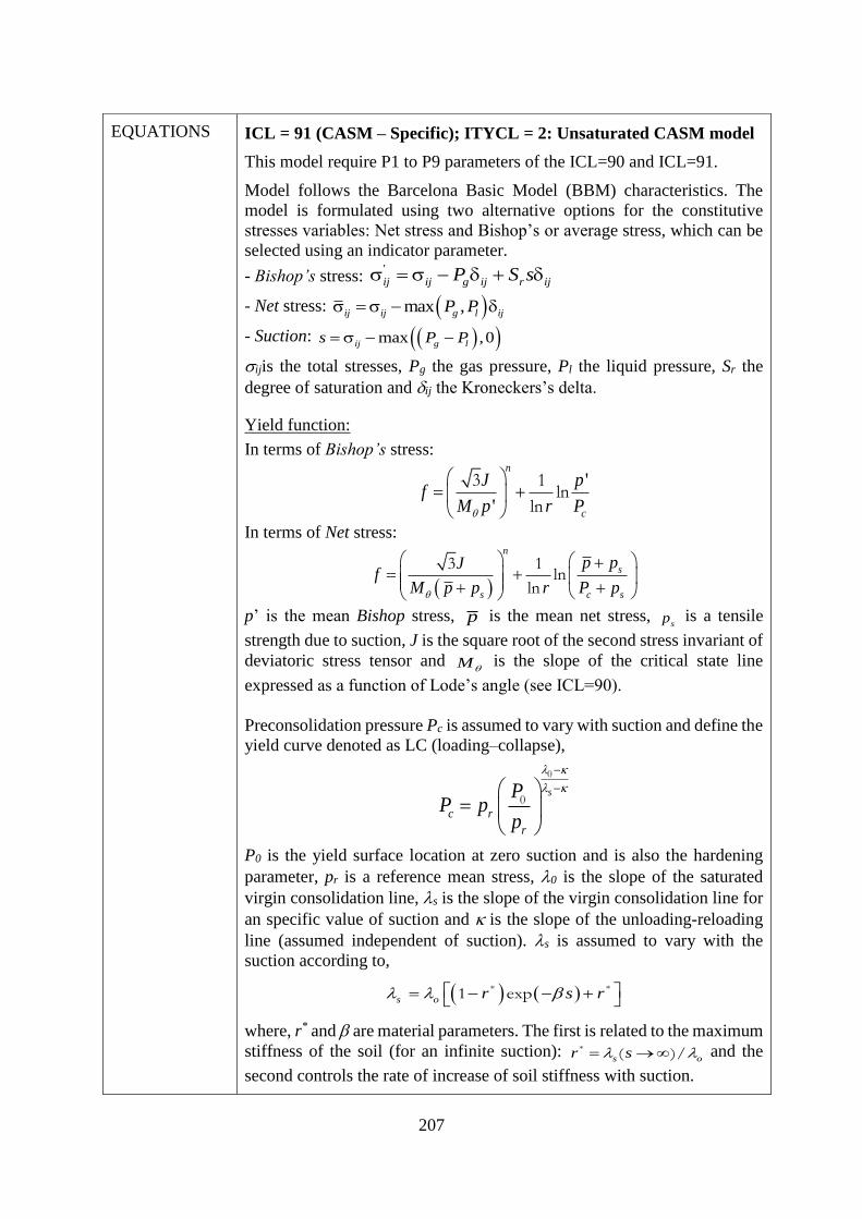
207
EQUATIONS ICL = 91 (CASM – Specific); ITYCL = 2: Unsaturated CASM model
This model require P1 to P9 parameters of the ICL=90 and ICL=91.
Model follows the Barcelona Basic Model (BBM) characteristics. The
model is formulated using two alternative options for the constitutive
stresses variables: Net stress and Bishop’s or average stress, which can be
selected using an indicator parameter.
- Bishop’s stress: '
ij ij g ij r ijP S s
- Net stress: max ,ij ij g l ijP P
- Suction: max ,0ij g ls P P
ijis the total stresses, Pg the gas pressure, Pl the liquid pressure, Sr the
degree of saturation and ij the Kroneckers’s delta.
Yield function:
In terms of Bishop’s stress:
3 1 'ln
' ln
n
c
J pf
M p r P
In terms of Net stress:
3 1
lnln
n
s
s c s
p pJf
M p p r P p
p’ is the mean Bishop stress, p is the mean net stress, s
p is a tensile
strength due to suction, J is the square root of the second stress invariant of
deviatoric stress tensor and M is the slope of the critical state line
expressed as a function of Lode’s angle (see ICL=90).
Preconsolidation pressure Pc is assumed to vary with suction and define the
yield curve denoted as LC (loading–collapse),
s
c r
r
PP p
p
0
0
P0 is the yield surface location at zero suction and is also the hardening
parameter, pr is a reference mean stress, 0 is the slope of the saturated
virgin consolidation line, s is the slope of the virgin consolidation line for
an specific value of suction and is the slope of the unloading-reloading
line (assumed independent of suction). s is assumed to vary with the
suction according to,
* *1 exps o
r s r
where, r* and are material parameters. The first is related to the maximum
stiffness of the soil (for an infinite suction): * ( )/s o
r s and the
second controls the rate of increase of soil stiffness with suction.

208
Net stress formulation requires an explicit variation of apparent cohesion
with suction. The increase in cohesion follows a linear relationship with
suction,
s sp k s
where sk is a scalar variable.
Plastic potential:
Three options are available for the flow rule. An scalar variable is
introduced to select a particular option as follow,
Flow_rule = 1. Non associated flow rule following the stress-dilatancy
relation of Rowe (see ICL=90 ITYCL=1)
Flow_rule = 2. Non associated flow rule to fit an one-dimensional
consolidation stress path (K0)
'
3 1 'ln
' ln
n
c
J pg
M p r P
with
*
1 * *
6 32
3 6 3
n n
n
M M M
M M
Flow_rule = 3. Associated flow rule (f=g)
Hardening parameter:
Isotropic hardening is controlled by the plastic volumetric strains ( p
vd )
through, po
o v
o
P eP d
1d
Elastic behaviour:
Elastic behaviour is the same as defined in ICL=90 ITYCL=1. However,
net stress formulation requires an explicit relation to consider the effect of
suction on volumetric elastic strains, through the incorporation of the
elastic compressibility parameter for changes in suction, s ,
e,s
ij
1d d δ d δ
1 ( ) 3
sij ij
atm s
s se s p K
Where sK is the Bulk modulus for changes in suction. If Bishop’s stress
is configured, the effect of suction on volumetric elastic strains is accounted
for via the variation in Bishop’s stress with suction. Elastic strain
increments are computed using the following equations for Net stress
approach and Bishop’s stress approach, respectively.
2 - 3 1 1d = d d d
6 2 3
e
ij ij ij ij
s
G Kp s
KG G K
2 - 3 1
d = d d '6 2
e
ij ij ij
G Kp Sr s
KG G

209
CODES in ROOT_gen.dat
ICL = 90, 91 (Mechanical data 3) ITYCL = 1, 2 ,3, 4
DESCRIPTION Clay and Sand model for soils (CASM)
EQUATIONS ICL = 91 (CASM – Specific); ITYCL = 3: Cemented CASM model
This model require P1 to P9 of ICL = 90 and P1 to P7 of ICL = 91
Cemented CASM model is based on the formulation for cemented soils
proposed by Gens & Nova (1993), in which a new state variable denoted
as ‘bonding’ b is incorporated.
Yield function:
'
( ' )3 1ln
( ' ) ln
n
t
t c t
p pJf
M p p r P p
c o
t o t
P P b
p P b
' '
' '
1
Where, b is a non-dimensional variable that represents the degree of
bonding. oP '
is the preconsolidation pressure of the unbonded material. cP '
controls the yielding of the bonded soil in isotropic compression and tp '
is
related to the cohesion and tensile strength of the material; αt is a parameter.
Both cP '
and tp increase with the magnitude of bonding. The unbonded
behaviour is recovered when b goes to zero.
The function defining the reduction of bonding (b) with increased
degradation and the relationship controlling the evolution of degradation in
response to plastic strains, are: 0( )
0
1 2
h h
p p
v q
b b e
dh h d h d
The above expressions ensure that degradation increases monotonically,
independently of the sign of the plastic strains. h1 y h2 are material
parameters (greater than zero) defining the rate of degradation. p
vd and
p
qd are the plastic volumetric strain increment and plastic deviatoric strain
increment, respectively.
The three options for the plastic potential used in the ICL = 91 ITYCL = 2
(Unsaturated model) are also available for this model.
Hardening parameter:
Either a volumetric hardening law or a combined volumetric and shear
hardening law can be used for this propose. If a combined hardening is
adopted, then:
'
0
' * *
0
1 p p
v q
dPd d
P
which reduces to the usual volumetric hardening law if it set 0 . is
a new constant introduced to control the relative contribution of the
incremental plastic deviatoric strain (p
qd ) to the rate of change of the
hardening parameter ( P '
0 ).
Elastic behaviour is the same as defined in ICL = 90; ITYCL = 1.

210
CODES in
ROOT_gen.dat
ICL = 90, 91 (Mechanical data 3) ITYCL = 1, 2 ,3, 4
DESCRIPTION Clay and Sand model for soils (CASM)
EQUATIONS ICL = 91 (CASM – Specific); ITYCL = 4: Double hardening soil model
(DHSM)
This model require P1 to P9 of ICL = 90 and P1 to P8 of ICL = 91
The model involves two plastic mechanisms: a plastic volumetric-driven
mechanism with isotropic hardening, by means of the use of the CASM
yield surface (ICL=90), and a plastic shear-driven mechanism that gives
rise to a nonlinear stress-strain relationship of a hyperbolic type, by the use
of a shear yield surface based on the Hardening Soil Model (HSM) (Schanz
et al., 1999).
Yield functions:
- Volumetric yield surface: CASM surface (see ICL = 1; ITYCL = 1)
- Shear yield surface:
s p
ur
a
J Jf
E EJ
J
50
1 2
1
with:
' ' cot ' ( ) sin ' and ( )
sin sin 'cos
3
f
a
f f
J p c gJ g
R R
aJ is the asymptotic value of the shear strength, Rf stands for the relation
between the ultimate deviatoric stress, fJ , and the asymptotic stress, a
standard setting is Rf = 0.9.p is the hardening parameter of the shear yield
surface and corresponds to the plastic deviatoric strain (p
d ), as is described
in the next section.
p'
J
P'o
Elastic Region
CASM yield surface
Shear yield surface
Mohr-Coulomb failure line
fs
fc
p

211
50E is a secant stiffness modulus for primary loading and ur
E is a secant
stiffness modulus for elastic unloading and reloading, these modulus are
computed as,
50 50
' ' cot ' ' ' cot ' and
' cot ' ' cot '
m m
ref ref
ur urref ref
p c p cE E E E
p c p c
refE50 is a reference stiffness modulus corresponding to a reference confining
pressurerefp , usually taken equal to the atmospheric pressure (100 kPa)
and ref
urE is the secant reference modulus for unloading and reloading. The
amount of stress dependency is given by the power m, for soft clays m
usually is taken equal to 1.0 and for sand, m lies in the range between 0.35
and 0.65.
Plastic potentials:
A non-associative flow rule is used for the shear yield surface which has
the following form,
p p
v md g d
where mg is a function of mobilized dilatancy angle, m
, and
Lode’s angle, , as,
mm
m
g
sin( )
sin sincos
3
The mobilized dilatancy angle, m
, is defined as,
m csm
m cs
sin sinsin
1 sin sin
Axial strain
De
via
toric s
tre
ss
-
1
Eur
150E
1
1 3
qa
fq
asymptote
failure line

212
cs is the friction angle at the critical state and m
is the mobilized
friction angle. Material contracts for small stress ratios m cs , while
dilatancy occurs for high stress ratios m cs . Considering dense
materials contraction is excluded by taking 0m
for a mobilized friction
angle m cs .
The volumetric surface uses a non-associated flow rule, the plastic potential
is defined in the ICL = 90; ITYCL = 1.
Hardening parameters:
The hardening parameter of the shear surface, p , is the plastic deviatoric
strainp p
d . The plastic deviatoric strain rate is calculated as,
22p
dd dJ
1/2
2 22 2 2 22
3
p p p p p p p
d x y x z y z xy xz yzd d d d d d d d d d
where, J
2 is the second strain invariant of deviatoric strain tensor, p is the
integral of plastic deviatoric strain rates.
The hardening parameter of the volumetric yield surface is the so-called
preconsolidation pressure ( P '
0 ) defined in the ICL = 90; ITYCL = 1.
The two surfaces can be activated simultaneously and move together as in
a multi-surface plasticity problem, if the stress path reaches the intersection
between both surfaces.
Elastic behaviour of the DHSM is the same as in basic CASM model
defined in the ICL = 90; ITYCL = 1.
Enhanced model (E –DHSM):
For stiff materials an enhanced model (E-DHSM) can be used, which
allows the evolution of the shear yield surface until the volumetric yield
surface is engaged on the dry side of the critical state, providing the
simulation of softening controlled by the hardening/softening law of the
CASM. In this case, a simple linear variation of the strength parameters
with plastic deviatoric strain, p
d , is employed, as,
'' p
d csA
'' p
c d resc A c
where, A and cA are two input parameters. If these parameters are zero
the basic DHSM is recovered.

213
PARAMETERS FOR CASM – GENERAL ICL = 90; ITYCL = 1 (General: required for
ICL = 91, ITYCL = 2, 3, 4)
P1 - Poisson ratio
P2 - Slope of unload/reload compression curve
P3 - Slope of the normal compression curve
P4 r - Spacing ratio
P5 n - Shape parameter
P6 M - Slope of Critical State Line
P7 cs º Friction angle at CS (computed as a function of M). If cs=0,
the shape of the YS plots as a circle in the deviatoric plane)
P8-P9 - -
P10 Su MPa Undrained shear strength (optional). By default = 0
PARAMETERS FOR CASM – SPECIFIC ICL = 91; ITYCL = 2 (Unsaturated)
P1 Pr MPa Reference mean stress (LC curve)
P2 r Parameter to control infinite suction (LC curve)
P3 MPa-1 Parameter to control stiffness (LC curve)
P4 s Elastic stiffness due to suction
P5 ks - Parameter to account tensile strength due to suction
P6 iunsat - Indicator of stress option: (0: net stress; 1: Bishop’s stress)
P7 pt MPa Tensile strength for saturated conditions
P8 flow_rule -
Flow rule indicator:
1: Non-associated: Rowe
2: Non-associated: K0 fit. Parameter is required
3: Associated
P9 - Non-associated parameter in case of flow_rule option equal to 2.
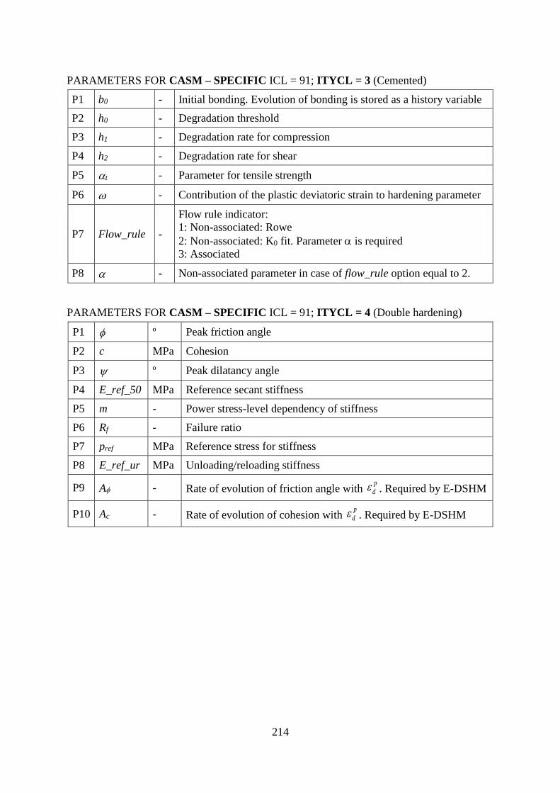
214
PARAMETERS FOR CASM – SPECIFIC ICL = 91; ITYCL = 3 (Cemented)
P1 b0 - Initial bonding. Evolution of bonding is stored as a history variable
P2 h0 - Degradation threshold
P3 h1 - Degradation rate for compression
P4 h2 - Degradation rate for shear
P5 t - Parameter for tensile strength
P6 - Contribution of the plastic deviatoric strain to hardening parameter
P7 Flow_rule -
Flow rule indicator:
1: Non-associated: Rowe
2: Non-associated: K0 fit. Parameter is required
3: Associated
P8 - Non-associated parameter in case of flow_rule option equal to 2.
PARAMETERS FOR CASM – SPECIFIC ICL = 91; ITYCL = 4 (Double hardening)
P1 º Peak friction angle
P2 c MPa Cohesion
P3 º Peak dilatancy angle
P4 E_ref_50 MPa Reference secant stiffness
P5 m - Power stress-level dependency of stiffness
P6 Rf - Failure ratio
P7 pref MPa Reference stress for stiffness
P8 E_ref_ur MPa Unloading/reloading stiffness
P9 A - Rate of evolution of friction angle with p
d . Required by E-DSHM
P10 Ac - Rate of evolution of cohesion with p
d . Required by E-DSHM

215
HISTORY VARIABLES:
The CASM’s family of constitutive models (ICL = 90, 91) use the following history variables.
Output variables can be visualized in the Post-process interface of GID.
Model Hist_var Description Type
ICL = 90
(ITYCL 1)
General
CASM
model
1 P0 (MPa): Evolution of preconsolidation pressure Input/Output
2 F: Value of the yield function Internal
3 e: Void ratio Internal
4 Id_F1: Indicator of plasticity Internal
ICL = 91
(ITYCL 2)
Unsaturated
CASM
model
1 P0 (MPa): Evolution of preconsolidation pressure Input/Output
2 s: Suction Output
3 e: Void ratio Internal
4 Pc (MPa): Evolution of preconsolidation
pressure due to suction Output
5 ps (MPa): Evolution of tensile strength due to
suction Output
5 F: Value of the yield function Internal
6 Id_F1: Indicator of plasticity Internal
ICL = 91
(ITYCL 3)
Cemented
CASM
model
1 P0 (MPa): Evolution of preconsolidation pressure Input/Output
2 Pc (MPa): Evolution of preconsolidation
pressure due to bond Internal
3 pt (MPa): Evolution of tensile strength due to
bond Output
4 b: Evolution of bonding Input/Output
5 h: Evolution of degradation rate Output
6 F: Value of the yield function Internal
7 e: Void ratio Internal
8 Id_F1: Indicator of plasticity Internal
ICL = 91
(ITYCL 4)
Double
hardening
CASM
model
1 P0 (MPa): Evolution of preconsolidation pressure
(volumetric surface) Input/Output
2 p : Evolution of plastic shear strain
(deviatoric surface) Output
3 F1: Value of the volumetric yield function Internal
4 F2: Value of the shear yield function Internal
5 c: Evolution of cohesion with plastic strain Internal
6 : Evolution of friction angle with plastic strain Internal
7 e: Void ratio Internal
8 Id_F1: Indicator of plasticity (volumetric
surface)Internal
9 Id_F2: Indicator of plasticity (deviatoric surface) Internal

216
The input variable (P0) is introduced as initial condition on surfaces/volumes in the conditions
window of GiD. Void ratio (e) is computed internally as a function of porosity.
Hist_var 1 Po MPa Evolution of preconsolidation mean stress for
saturated soil
The evolution of some history variables can be visualized as an output in Post-process GID
interface.
Note: Effective stresses plotted in the Post-process GID interface correspond with Terzaghi's
effective stresses for saturated conditions (ITYCL = 1, 3, 4). For ITYCL = 2 (Unsaturated
CASM model) if the indicator iunsat (P6 of ICL = 91; ITYCL = 2) is equal to 0, net stress are
plotted, if iunsat = 1, Bishop’s effective stresses are plotted. Stress and strain invariants follow
the soil mechanics notation (positive for compression).
_________

217
CODE_BRIGHT. CONSTITUTIVE LAWS
This chapter contains the different models available and the corresponding parameters required
by each model. The following constitutive laws are available:
HYDRAULIC AND
THERMAL CONSTITUTIVE
MODELS (a)
RETENTION CURVE
INTRINSIC PERMEABILITY
LIQUID PHASE RELATIVE
PERMEABILITY
GAS PHASE RELATIVE
PERMEABILITY
DIFFUSIVE FLUXES OF MASS
DISPERSIVE FLUXES OF
MASS AND ENERGY
CONDUCTIVE FLUX OF HEAT
MECHANICAL CONSTITUTIVE MODELS
ELASTICITY (b)
NONLINEAR ELASTICITY (b)
VISCOPLASTICITY FOR SALINE MATERIALS
(b)
VISCOPLASTICITY FOR SATURATED SOILS
AND ROCKS (b)
VISCOPLASTICITY - GENERAL (b)
DAMAGE-ELASTOPLASTIC MODEL FOR
ARGILLACEOUS ROCKS (c)
THERMOELASTOPLASTIC MODEL FOR SOILS
(d)
BARCELONA EXPANSIVE MODEL FOR SOILS
(e)
CASM’s FAMILY MODELS (f)
PHASE PROPERTIES (a)
SOLID PHASE PROPERTIES
LIQUID PHASE PROPERTIES
GAS PHASE PROPERTIES
EXCAVATION PROCESS (g)

218
VI.g. EXCAVATION/CONSTRUCTION PROCESS
EXCAVATION/CONSTRUCTION
CODES ICL = 50 ITYCL = 1
DESCRIPTION Flag for excavation and construction process
EQUATIONS Options:
- Active material (default option) → P1 = 0
- Inactive material: material that has not yet been constructed or material
that has been excavated → P1 = -1
- Construction: the material is constructed with its gravity increased
linearly during the interval → P1 = 1
After the construction interval is finished, the constructed material
automatically will be considered active in the next interval → P1 = 0
- Smooth excavation (P1 = 2): the material excavated becomes elastic
and its stress is relaxed smoothly according to the following equation:
𝜎𝑡 = 𝜎𝑡𝑖𝑚𝑒𝑖 (𝑨 − 𝑩 [𝑡 − 𝑡𝑖𝑚𝑒𝑖
𝑡𝑖𝑚𝑒𝑓 − 𝑡𝑖𝑚𝑒𝑖]𝒏
)
where: timei = interval initial time
timef = interval final time
t = current time
𝜎𝑡 = stress in time t
𝜎𝑡𝑖𝑚𝑒𝑖 = stress at the initial time of the interval
A is a user-defined parameter taking values between 0 and 1
B is a user-defined parameter taking values between 0 and 1
n is a user-defined exponent
If A = 1 (default value), then the excavated material is relaxed from its
current stress (recommended). If A < 1, then the excavated material is
relaxed from a lower stress level.
If B = 1 (default value), then the excavated material is relaxed until zero
(usual case). If B < 1, then the excavated material is relaxed until a
stress level higher than zero (useful in some cases, like e.g. installing
support in a 2D model after a given relaxation).
If n = 1 (default value), then the excavated material is relaxed linearly
(recommended), but it could also be relaxed in an accelerated (n > 1) or
decelerated manner (n < 1) during the interval.
After the excavation interval is finished, the excavated material
automatically will be considered inactive in the next interval, and thus
will not be considered in the calculation process.
Finally, if P7 = 1, then volumetric deformation effects on hydraulics are
neglected. As a consequence, the numerical performance of the model is
better, especially during excavation.

219
PARAMETERS FOR ITYCL = 1
P1 Option
-1: material is inactive.
0: material is active (default option).
1: material is constructed (during the current time interval
with gravity increasing linearly with time). After construction
interval, P1 is set to 0 internally.
2: material is excavated smoothly (during the current time
interval). After excavation interval, P1 is set to -1 internally.
P2 Properties
IMATEQ: Material index (integer) of the material
(previously defined) that has the same properties as the
current one. Normally, some construction or excavation
layers may have the same properties.
P2 = 0, properties should be given for the current material.
P2 = IMATEQ, properties from the material
IMAT = IMATEQ will be copied for this material.
P3 Smoothing exponent n May be used when P1 = 2. Default value = 1
P4 Smoothing parameter A May be used when P1 = 2. Default value = 1
P5 Smoothing parameter B May be used when P1 = 2. Default value = 1
P7 M→H uncoupled If P7=1, then volumetric deformation effects on hydraulics
are neglected.
By default (P1 = 0), the material is active and all the parameters read are used by the
programme. When P1 = -1, elements having the material number are not assembled.
As an example, Figure VIg.1 show the two main steps followed in an excavation problem
(tunnel). In the first interval time is necessary to impose the initial conditions before excavation.
In this time interval, the material is active (P1 = 0). In the second interval time, the relaxation
of stresses occurs due to excavation of the material, parameter P1 is equal to -1 (or alternatively
P1=2 using the smooth excavation feature).
During the excavation interval, it is necessary to impose the ambient conditions in the tunnel,
namely, pore water pressure in equilibrium with atmospheric pressure, pore air phase in
equilibrium with the relative humidity and temperature equilibrium. When setting these
ambient conditions during excavation, it is recommended to use a ramp and/or a small value of
the corresponding gamma parameter, to avoid numerical issues.

220
Figure VIg.1. Illustration of the two main steps followed during excavation problem
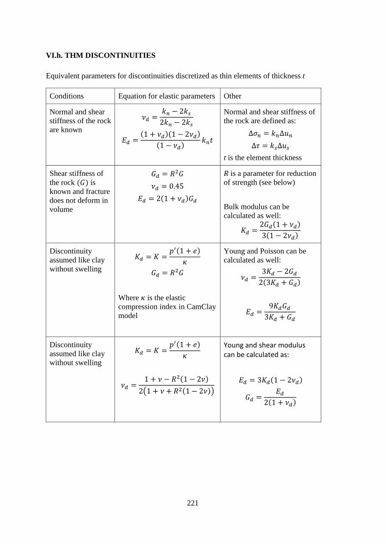
221
VI.h. THM DISCONTINUITIES
Equivalent parameters for discontinuities discretized as thin elements of thickness t
Conditions Equation for elastic parameters Other
Normal and shear
stiffness of the rock
are known
𝜈𝑑 =𝑘𝑛 − 2𝑘𝑠2𝑘𝑛 − 2𝑘𝑠
𝐸𝑑 =(1 + 𝜈𝑑)(1 − 2𝜈𝑑)
(1 − 𝜈𝑑)𝑘𝑛𝑡
Normal and shear stiffness of
the rock are defined as:
∆𝜎𝑛 = 𝑘𝑛∆𝑢𝑛
∆𝜏 = 𝑘𝑠∆𝑢𝑠
t is the element thickness
Shear stiffness of
the rock (𝐺) is
known and fracture
does not deform in
volume
𝐺𝑑 = 𝑅2𝐺
𝜈𝑑 = 0.45
𝐸𝑑 = 2(1 + 𝜈𝑑)𝐺𝑑
R is a parameter for reduction
of strength (see below)
Bulk modulus can be
calculated as well:
𝐾𝑑 =2𝐺𝑑(1 + 𝜈𝑑)
3(1 − 2𝜈𝑑)
Discontinuity
assumed like clay
without swelling
𝐾𝑑 = 𝐾 =𝑝′(1 + 𝑒)
𝜅
𝐺𝑑 = 𝑅2𝐺
Where 𝜅 is the elastic
compression index in CamClay
model
Young and Poisson can be
calculated as well:
𝜈𝑑 =3𝐾𝑑 − 2𝐺𝑑2(3𝐾𝑑 + 𝐺𝑑)
𝐸𝑑 =9𝐾𝑑𝐺𝑑3𝐾𝑑 + 𝐺𝑑
Discontinuity
assumed like clay
without swelling
𝐾𝑑 = 𝐾 =𝑝′(1 + 𝑒)
𝜅
𝜈𝑑 =1 + 𝜈 − 𝑅2(1 − 2𝜈)
2(1 + 𝜈 + 𝑅2(1 − 2𝜈))
Young and shear modulus can be calculated as:
𝐸𝑑 = 3𝐾𝑑(1 − 2𝜈𝑑)
𝐺𝑑 =𝐸𝑑
2(1 + 𝜈𝑑)

222
Conditions Equation for plastic parameters
Cohesion and
friction angle are
known
𝑐𝑑′ = 𝑅𝑐′𝑠𝑜𝑖𝑙
𝜙𝑑′ = atan(𝑅 tan𝜙′𝑠𝑜𝑖𝑙)
R is a reduction factor for
strength properties
Slope of critical state
and cohesion term
are known
𝑀𝑑 = 𝑅𝑀
𝑝𝑠𝑑 = 𝑅(𝑝𝑠0 + 𝑘𝑠)
In general, the corresponding intrinsic permeability is easy to calculate from transmissivity, if
this later is known.
For soils, both intrinsic permeability and retention curve depend on porosity. If permeability
and retention curve depend on porosity, it is sufficient to consider a larger porosity for the
interface in order to increase permeability and reduce air entry value. The following options
can be used:
Exponential equation. In the case presented here, increasing porosity of the interface
zone by 50% may be sufficient to produce this effect.
Kozeny equation. It is also a function of porosity but it does not include parameters
except a value of permeability for a given porosity.
Other alternatives can be considered if variation should be larger (cubic law) and more
information of the discontinuity.

223
CODE_BRIGHT. REFERENCES
Formulation and numerical methods
Allen, M.B. and Murphy C.L. (1986): A Finite-Element Collocation Method for Variably
Saturated Flow in Two Space Dimensions, Water Resources Research, 22, no. 11:
1537:1542.
Altunin, VV & Sakhabetdinov, MA (1972). Viscosity of liquid and gaseous carbon dioxide at
temperatures 220-1300 K and pressure up to 1200 bar. Teploenergetika, 8:85-89.
Celia, M.A., Boulotas, E.T. and Zarba, R. (1990): A General Mass Conservative Numerical
Solution for the Unsaturated Flow Equation, Water Resources Research, 26, no. 7:
1483:1496.
Chen, G., Ledesma, A. (2009). Coupled Thermohydromechanical Modeling of the Full-Scale
In Situ Test "Prototype Repository. Journal of geotechnical and geoenvironmental
engineering, vol. 135, núm. 1, p. 121-132.
Garcia, J.E. (2003). Fluid Dynamics of Carbon Dioxide Disposal into Saline Aquifers. PhD
thesis, University of California, Berkeley.
Gerard, P., Léonard, A., Masekanya, J.-P., Charlier, R. and Collin, F. (2010), Study of the soil–
atmosphere moisture exchanges through convective drying tests in non-isothermal
conditions. Int. J. Numer. Anal. Meth. Geomech., 34: 1297–1320. doi:10.1002/nag.866
Hughes, T. J. R. (1980): Generalisation of Selective Integration Procedures to Anisotropic and
Nonlinear Media, Int. J.Num. Meth. Eng. 15, 1413-1418.
Huyakorn, P.S. and Pinder, G.F. (1983): Computational Methods in Subsurface Flow,
Academic Press, Inc. ISBN 0-12-363480-6.
Huyakorn, P.S., Springer, E.P., Guvanasen, V. and Wadsworth, T.D. (1986): A Three-
dimensional Finite-Element Model for Simulating Water Flow in Variably Saturated
Porous Media, Water Resources Research, 22, no. 13 : 1790:1808}.
McCutcheon, S.C., Martin, J.L, Barnwell, T.O. Jr. 1993. Water Quality in Maidment, D.R.
(Editor). Handbood of Hydrology, McGraw-Hill, New York, NY (p. 11.3).
Milly, P.C.D. (1984): A mass-conservative procedure for time stepping in models of
unsaturated flow, in Proceedings Fifth International Conference on Finite Elements in
Water Resources, edited by J. P. Laible et al., Springer-Verlag, New York: 103-112.
Olivella, S., J. Carrera, A. Gens, E. E. Alonso, (1994). Non-isothermal Multiphase Flow of
Brine and Gas through Saline media. Transport in Porous Media, 15, 271:293
Olivella, S., A. Gens, J. Carrera, E. E. Alonso, (1996), Numerical Formulation for a Simulator
(CODE_BRIGHT) for the Coupled Analysis of Saline Media, Engineering
Computations, Vol. 13, No 7, pp: 87-112.
Olivella, S., J. Carrera, A. Gens, E. E. Alonso. (1996) Porosity Variations in Saline Media
Caused by Temperature Gradients Coupled to Multiphase Flow and
Dissolution/Precipitation. Transport in Porous Media, 25:1-25.
Pini, G. and Gambolatti, G. (1990), Is a simple diagonal scaling the best pre-conditioner for
conjugate gradients on super-computers? Advances in Water Resources.
Sonnelveld, P., (1989), CGS, A fast Lanczos-type solver for non-symmetric linear systems,
SIAM J. Sci. Stat. Comput., 10, 36-52.

224
Spycher, N, Pruess, K & Ennis-king, J (2003). CO2-H2O Mixtures in the Geological
Sequestration of CO2. I. Assessment and calculation of mutual solubilities from 12 to
100°C and up to 600 bar. Geochim. Cosmochim. Acta, 67:3015-3031.
Voss, C.I. (1984): SUTRA Users's Guide, U.S. Geological Survey, Water Resources
investigations, Report 48-4369.
Van der Vorst, Henk (1990), Iterative methods for the solution of large systems of equations
on super-computers, Advances in Water Resources, Vol. 13, No. 3, 137-146.
Viscous/creep models
Olivella, S.; A. Gens, J. Carrera, and E. E. Alonso (1993): Behaviour of Porous Salt Aggregates.
Constitutive and Field Equations for a Coupled Deformation, Brine, Gas and Heat
Transport Model. The Mechanical Behaviour of Salt III, Trans Tech Publications, pp.
269:283. ISBN 0-87849-100-7.
Olivella, S., A. Gens, J. Carrera, E. E. Alonso (1996) Analysis of Creep Deformation of
Galleries Backfilled with Porous Salt Aggregates. The Mechanical Behaviour of Salt
IV, Trans Tech Publications, 379:386.
State surface approach
Fredlund, D.G., Morgenstern, N.R., 1977. Stress state variables for unsaturated soils. J Geotech
Engng Div, 103(GT5):447-466.
Lloret, A. & Alonso, E., 1985. State surfaces for partially saturated soils. Proc. 11th Int. Conf.
Soil Mech. Fdn Engng, San Franciso, vol. 2, pp. 557-562.
Matyas, E.L. & Radhakrishna, H.S., 1968. Volume change characteristics of partially saturated
soils, Géotechnique, 18(4):432-448.
Elastoplastic model for unsaturated soils
Alonso, E.E., Gens, A., Josa, A., 1990. A constitutive model for partially saturated soils.
Géotechnique 40(3):405-430.
Gens, A., Potts, D.M., 1988. Critical state models in computational geomechanics. Eng Comp,
5(3):178-197.
Ledesma, A., Chan, A.H.C, Vaunat, J., Gens, A., 1995. Finite Element formulation of an elasto-
plastic model for partially saturated soils. In: Owen, D.R.J., Oñate, E. (Eds.) Proc. 4th Int.
Conf. on Computational Plasticity, Pineridge Press, Swansea, pp. 1677-1688.
Maâtouk, A., Leroueil, S., La Rochelle, P., 1995. Yielding and critical state of a collapsible
unsaturated silty soil. Géotechnique, 45(3):465-477.
Ohmaki, S., 1982. Stress-strain behaviour of anisotropically, normally consolidated cohesive
soil. In: Dungar, R., Pande, G.N., Studer, J.A. (Eds), Proc. 1st Int. Symp. on Num. Models
in Geomechanics, Balkema, Rotterdam, pp. 250-269.
Roscoe, K.H., Burland, J.B., 1968. On the generalized stress-stain behaviour of the 'wet' clay.
In: Heyman, J.,Leckie, F.A. (Eds.), Engineering Plasticity, Cambridge University Press,
Cambridge, pp. 535-609.
Sloan, S.W., 1987. Substepping schemes for the numerical integration of elastoplastic stress-
strain relations. Int J Num Methods Engrg, 24(5), 893-911.
Wheeler, S.J., Sivakumar, V., 1995. A elasto-plastic critical state framework for unsaturated
soil. Géotechnique 45(1):35-53.
Wood, D.M., 1990. Soil behaviour and critical state soil mechanics. Cambridge University
Press, Cambridge.

225
Thermoelastoplastic model for unsaturated soils
Hueckel, T. & Borsetto, M. 1990. Thermoplasticity of saturated soils and shales: constitutive
equations. Jnl. Geot. Eng. ASCE, 116: 1765-1777.
Hueckel,T.& Baldi, G. 1990.Thermoplasticity of saturated clays: experimental constitutive
study. Jnl. Geot. Eng.ASCE,116:1778-1796.
Hueckel,T. & Pellegrini,R.(1991). Thermo-plastic modelling of untrained failure of saturated
clay due to heating. Soils and Found., 3:1-16.
García Molina. A., Gens, Añ & Olivella, O. 1996. Un modelo constitutivo para suelos no
saturados sometidos a variaciones térmicas: formulación, implementació y aplicaciones. In
Doblaré, M., Correas, J.M., Alarcón E., Gavete, L. & Pastor, M. (Eds): Proc. III Congreso
de Métodos Numéricoas en Ingeniería, pp.502-512.
Gens, A. 1995. Constitutive laws. In Gens, A., Jouanna, P. & Schrefler, B. (Eds): Modern issues
in non-saturated soils, Springer-Verlag.
Visco-plastic model for unsaturated soils
Perzyna, J.K. (1966). Fundamental problems in viscoplasticity. Adv. Appl. Math. 9, 243–377.
Desai, C.S and Zhang, D. (1987. Viscoplastic model for geologic materials with generalized
flow rule. Int. J. Num. Anal. Methods in Geomech. Vol 11, issue 6, pp. 603-260.
Sánchez, Marcelo. 1997. Implementation of VP model by Desai in CB. Used to simulate triaxial
tests under drained conditions. Master’s thesis, UPC, January 1997.
Molist, Jordi. 1997. Extension of the VP model by Desai to unsaturated soils. Graduation thesis.
UPC. September 1997.
Oldecop, L.A. and Alonso, E.E. 2001 A constitutive model for rockfill compressibility.
Géotechnique 51, No.2, pp 127-239.
Zandarin, Maria Teresa. 2010. Thermo-hydro-mechanical analysis of joints a theoretical and
experimental study. PhD Thesis. UPC. Barcelona.
Damage-elastoplastic model for argillaceous rocks
Carol, I., Rizzi E. & Willam K. 2001. “On the formulation of anisotropic elastic degradation.
1. Theory based on a pseudo-logarithmic damage tensor rate”, Int. J. Solids Struct., 38:
491-518.
Hoek, E. & Brown, E. T. 1980. “Empirical strength criterion for rock masses”, Journal of the
Geotechnical Engineering Division, 106: 1013-1035 .
Sloan, S. W. & Booker, J. R. 1986. Removal of singularities in Tresca and Mohr-Coulomb yield
functions. Communications in Applied Numerical Methods, 2: 173-179.
Vaunat, J. & Gens, A. 2003. Bond degradation and irreversible strains in soft argillaceous rock.
In: Cullighan, P.J., Einstein, H.H. & Whittle, A. (Eds.) “Proceedings of 12th Panamerican
Conference on Soil Mechanics and Geotechnical Engineering”, 23th –25th June 2003,
Boston, United-State, Pub. VGE, ISBN 3-7739-5985-0, vol. 1, pp. 479-484.
Barcelona expansive model (BExMo)
Alonso, E.E., Vaunat, J., & Gens, A. 1999. “Modelling the mechanical behaviour of expansive
soils ”, Engng. Geol. 54 Nos 1-2, 173-183.
Pinyol, N., Vaunat, J., & Alonso, E.E. 2007. “A constitutive model for soft clayey rocks that
includes weathering effects”. Géotechnique 57, No.2, 137-151.

226
CASM’s family models
Alonso, E.E., Gens, A., Josa, A., 1990. A constitutive model for partially saturated soils.
Géotechnique 40(3):405-430.
Gens, A. & Nova, R. (1993). Conceptual bases for a constitutive model for bonded soils and
weak rocks. In Geotechnical Engineering of Hard Soils-Soft Rocks, Athens, Greece,
Anagnostopoulos et al. (eds.) Rotterdam: Balkema, 577-583.
González, N.A. (2011). Development of a family of constitutive models for Getoechnical
applications. PhD Thesis. UPC. Barcelona.
Schanz, T., Vermeer, P.A. & Bonnier, P.G. (1999). Formulation and verification of the
Hardening-Soil Model. Beyond 2000 in Computational Geotechnics, pages 281–290.
Balkema, Rotterdam.
Sheng, D., Sloan S.W., & Yu, H.S. (2000). Aspects of finite element implementation of critical
state models. Computational Mechanics 26, 185-196.
Yu, H.S. (1988). CASM: A unified state parameter model for clay and sand. International
Journal of Numerical and Analytical Methods in Geomechanics, 22, 621-653.
Other
Chow, V. T., Maidment, D. R., and Mays, L. W. (1988). Applied Hydrology, McGraw-Hill
Gens, A. , A.J. Garcia-Molina, S. Olivella, E. E. Alonso, F. Huertas. (1998) Analysis of Full
Scale In-situ Heating Test Simulating Repository Conditions. Int. Journal for Numerical and
Analitical Methods in Geomechanics. 22:515-548.
___________________________________